Embed Size (px)
Citation preview
WET-GAS COMPRESSION IN TWIN-SCREW MULTIPHASE PUMPS
A Thesis
by
EVAN CHAN
Submitted to the Office of Graduate Studies of
Texas A&M University in partial fulfillment of the requirements for the degree of
MASTER OF SCIENCE
December 2006
Major Subject: Petroleum Engineering
WET-GAS COMPRESSION IN TWIN-SCREW MULTIPHASE PUMPS
A Thesis
by
EVAN CHAN
Submitted to the Office of Graduate Studies of
Texas A&M University in partial fulfillment of the requirements for the degree of
MASTER OF SCIENCE
Approved by: Chair of Committee, Stuart L. Scott Committee Members, Daulat Mamora Charles Glover Head of Department, Stephen Holditch
December 2006
Major Subject: Petroleum Engineering
iii
ABSTRACT
Wet-Gas Compression in Twin-Screw Multiphase Pumps.
(December 2006)
Evan Chan, B.S., Brown University
Chair of Advisory Committee: Dr. Stuart L. Scott
Multiphase pumping with twin-screw pumps is a relatively new technology that
has been proven successful in a variety of field applications. By using these pumps to
add energy to the combined gas and liquid wellstream with minimal separation, operators
have been able to reduce capital costs while increasing overall production. In many
cases, such as subsea operations, multiphase pumping is the only viable option to make
remote wells economic.
Despite their many advantages, some problems have been encountered when
operating under conditions with high gas volume fractions (GVF). Twin-screw
multiphase pumps experience a severe decrease in efficiency when operating under wet-
gas conditions, GVF over 95%. Field operations have revealed severe vibration and
thermal issues which can lead to damage of the pump internals, requiring expensive
maintenance. The research presented in this thesis seeks to investigate two novel
methods of improving the performance of twin-screw pumps under wet-gas conditions.
The first involves increasing the viscosity of the liquid stream. We propose that
by increasing the viscosity of the liquid phase, the pump throughput can be increased.
Tests were conducted at high GVF using guar gel to increase the viscosity of the liquid
phase. Along with results from a multiphase pump model the pump behavior under wet-
gas conditions with increased liquid viscosity was evaluated. The experimental results
indicate that at high GVF, viscosity is not a dominant parameter for determining pump
performance. Possible reasons for this behavior were proposed. These results were not
predicted by current pump models. Therefore, several suggestions for improving the
model’s predictive performance were suggested.
The second method is the direct injection of liquid into the pump casing. By
selectively injecting liquid into specific pump chambers, it is believed that many of the

iv
vibration issues can be eliminated with the added benefit of additional pressure boosting
capacity. Since this method requires extensive mechanical modifications to an existing
pump, it was studied only analytically. Calculations were carried out that show that
through-casing liquid injection is feasible. More favorable pressure profiles and
increased boosting ability were demonstrated.

v
DEDICATION
I dedicate this work to my family.

vi
ACKNOWLEDGEMENTS
I would like to thank Dr. Scott for his guidance and for making this work
possible. I would also like to thank Jason and Hemant with whom I shared many hours at
Riverside.
vii
TABLE OF CONTENTS Page
ABSTRACT……………………………………………………………...............…. iii
DEDICATION……………………………………………………………………… v
ACKNOWLEDGEMENTS……………………………………………………….. vi
TABLE OF CONTENTS…………………………………………………………… vii
LIST OF FIGURES………………………………………………………………… ix
LIST OF TABLES………………………………………………………………….. xiv
CHAPTER
I INTRODUCTION………………………………………………….....…… 1
II LITERATURE REVIEW: TWIN-SCREW PUMP MODELS……...…….. 5
2.1 Vetter et al. (1993)………………………………………………… 7 2.2 Egashira et al. (1996)……………………………………………… 9 2.3 Martin and Scott (2003)…………………………………………… 10 2.4 Cooper & Prang (2004)……………………………………………. 12 2.5 University of Hannover (2004)……………………………………. 13 2.6 Model Comparisons and Thermal Issues………………………….. 14
III METHODS FOR WET-GAS COMPRESSION…………………………... 15
3.1 Volumetric Efficiency……………………………………………... 15 3.2 Conventional Methods………...…………………………………... 16 3.3 Digressive Screws…………………………………………………. 17 3.4 High Viscosity Fluid Circulation….………………………….…… 18 3.5 High Viscosity Test Matrix………………………………………... 24 3.6 Through-casing Injection………………………………………….
25
IV EXPERIMENTAL FACILITY……..……………………………………...
27
4.1 Flow Loop Description…………………………………………….. 29 4.2 Data Acquisition…………………………………………………… 33
4.3 Viscosity Control…………………………………………………...
34
viii
CHAPTER Page
V HIGH VISCOSITY CIRCULATION................…………………………... 39
5.1 Pure Liquid Tests………………………………………………….. 40 5.2 100% GVF Tests…………………………………………………... 43 5.3 GVF Progression…………………………………………………... 45 5.4 Speed Comparison…………………………………………………. 47 5.5 Wet-gas Compression Tests………………………………………. 48 5.6 Model Verification………………………………………………… 51 5.7 Viscosity Correction……………………………………………….. 58
5.8 Conclusions and Recommendations……...………………………... 61
VI THROUGH-CASING INJECTION……………………….………………. 62
6.1 Injection Theory………………...…………………………………. 62 6.2 Feasibility Study………………..…………………………………. 67 6.3 Conclusions………………………………………………………... 77
VII SUMMARY OF CONCLUSIONS AND RECOMMENDATIONS 78
7.1 Pure-Liquid Tests……...…………………………………………... 78 7.2 Wet-gas Tests…………………..…………………………………. 78 7.3 Model Recommendations…………………………………………. 78 7.4 Experiment Recommendations……………………………………. 79 7.5 Through-casing Injection Feasibility……………………………... 79
NOMENCLATURE………………………………………………………………… 80
REFERENCES……………………………………………………………………... 81
APPENDIX A – STUDY OF TWIN-SCREW PUMP CLEARANCES…………… 85
APPENDIX B – 0% GVF DATA…………………………..………………………. 89
APPENDIX C – 70% GVF DATA…………………………..……………………... 93
APPENDIX D – 95% GVF DATA…………………………..……………………... 95
APPENDIX E – 100% GVF DATA…………………………..……………………. 99
VITA………………………………………………………………………………... 100

ix
LIST OF FIGURES FIGURE Page
1.1 Cut-away view of twin-screw pump internals (after Scharf et al.2)……….
1
2.1 Screw intermeshing and slip flow paths (after Martin8,9)..………………... 5
2.2 Simplified twin-screw model (after Vetter et al.10,11)..……………………. 7
2.3 Pressure profiles for single and two phase pumping (after Vetter et al.10,11) 8
2.4 Simplified pump model (after Martin8,9)...………………………………… 10
3.1 Conventional production process flow diagram (after Dick and Speirs5)……………………………………………………………………
16
3.2 Multiphase production process flow diagram (after Dick and Speirs5)……………………………………………………………………
17
3.3 Diagram of digressive screw………………………………………………. 17
3.4 Digressive screw test results (after Rohlfing and Muller-Link14)…………. 18
3.5 Viscosity effects on liquid flow rate (after Martin8,9)..……………………. 19
3.6 Reduced slip allows for more gas flow (after Martin8,9),,…………………. 20
3.7 Gas flow rate versus differential pressure for different liquid viscosities, pump speed 1350 RPM (after Singh6,7)..…………………………………...
20
3.8 Gas flow rate versus differential pressure for different liquid viscosities, pump speed 750 RPM (after Singh6,7)..…………………………………….
21
3.9 Nuovo Pignone, total flow rate versus differential pressure for different liquid viscosities, pump speed 1800 RPM…………………………………
22
3.10 Nuovo Pignone, total flow rate versus differential pressure for different liquid viscosities, pump speed 1200 RPM…………………………………
22
3.11 Improvement in total flow rate with increased viscosity………………….. 23
3.12 Theoretical pressure profile with through-casing injection….…………….. 25
x
FIGURE Page
3.13 Diagram of injection timing problem…………..………………………….. 26
4.1 Bornemann MW-6.5zk-37 twin-screw pump with internal recirculation chamber…………………………………………………………………….
28
4.2 Rendition of Riverside test facility (Martin8,9)..…………………………… 28
4.3 Flow diagram of Riverside test facility (after Martin8,9)...………………… 29
4.4 Centrifugal charging pumps……………………………………………….. 30
4.5 Pressure equalization vessel……………………………………………….. 31
4.6 Metering section and mixing tee…………………………………………... 32
4.7 Backpressure control valve………………………………………………... 33
4.8 Gel concentration versus viscosity at different shear rates...……………… 34
4.9 Apparent viscosity (cP) versus shear rate (sec-1) for different gel concentrations…………………………………………................................
35
5.1 Liquid flow rate (GPM) versus differential pressure (psi) for four different viscosities and two pump speeds…………………………………………...
40
5.2 Volumetric efficiency (%) versus differential pressure (psi) at 1350 and 1700 RPM, liquid viscosity 1 cP…………………………………………...
41
5.3 Liquid flow rate (GPM) versus differential pressure (psi) for four different viscosities at 1350 RPM……………………………………………………
41
5.4 Slip flow rate (GPM) versus differential pressure (psi) for four different viscosities at 1350 RPM……………………………………………………
42
5.5 Liquid flow rate (GPM) versus differential pressure (psi) for four different viscosities at 1700 RPM……………………………………………………
43
5.6 Gas flow rate (GPM) versus differential pressure (psi) , 100% GVF for a 1 cP and 9 cP fluid……………………………………………………………
44
5.7 GVF progression, total flow rate (GPM) versus differential pressure (psi), 1 cP fluid at 1350 RPM…………………………………………………….
45
xi
FIGURE Page
5.8 GVF progression, total flow rate (GPM) versus differential pressure (psi), 1 cP fluid at 1700 RPM…………………………………………………….
46
5.9 Speed comparison, total flow rate (GPM) versus differential pressure (psi), 95% GVF…………………………………………………………….
47
5.10 Total flow rate (GPM) versus differential pressure (psi), 95% GVF, 1350 RPM………………………………………………………………………..
48
5.11 Total flow rate (GPM) versus differential pressure (psi), 95% GVF, 1700 RPM………………………………………………………………………..
49
5.12 Total flow rate (GPM) versus differential pressure (psi), 70% GVF, 1350 and 1700 RPM……………………………………………………………...
50
5.13 Model match, total flow rate (GPM) versus differential pressure (psi), 1350 RPM, 1 cP liquid……………………………………………………..
51
5.14 Model match, total flow rate (GPM) versus differential pressure (psi), 0% GVF, 1350 RPM, 1 cP liquid………………………………………………
52
5.15 Model match, total flow rate (GPM) versus differential pressure (psi), 70% GVF, 1350 RPM, 1 cP liquid…………………………………………
53
5.16 Model match, total flow rate (GPM) versus differential pressure (psi), 95% GVF, 1350 RPM, 1 cP liquid…………………………………………
53
5.17 Model match, total flow rate (GPM) versus differential pressure (psi), 1350 RPM, 9 cP liquid……………………………………………………..
54
5.18 Model match, total flow rate (GPM) versus differential pressure (psi), 1350 RPM, 24 cP liquid……………………………………………………
55
5.19 Model match, total flow rate (GPM) versus differential pressure (psi), 1350 RPM, 24 cP liquid, laminar flow only……………………………….
56
5.20 Model match, total flow rate (GPM) versus differential pressure (psi), 1350 RPM, 24 cP liquid, turbulent flow only……………………………...
57
5.21 Viscosity match, total flow rate (GPM) versus differential pressure (psi), 1350 RPM, 9 cP……………………………………………………………
58
5.22 Viscosity match, total flow rate (GPM) versus differential pressure (psi), 1350 RPM, 24 cP………………………………………………………….. 59
xii
FIGURE Page
5.23 Viscosity match, total flow rate (GPM) versus differential pressure (psi), 1350 RPM, 40 cP…………………………………………………………..
59
5.24 Corrected viscosity match, total flow rate (GPM) versus differential pressure (psi), 1350 RPM, 95% GVF……………………………………...
60
6.1 Pressure profiles (psig), differential pressure 200 psi, 1800 RPM (after Martin8)…………………………………………………………………….
63
6.2 Liquid volume in chambers (gal), differential pressure 200 psi, 1800 RPM (after Martin8)………..……………………………………………………..
64
6.3 Simplified injection model………………………………………………… 65
6.4 Pressure profiles (psig) with injection, 90% GVF, differential pressure 200 psi, 1800 RPM…………………………………………………………
67
6.5 Liquid volume in chambers (gal) with injection, 90% GVF, differential pressure 200 psi, 1800 RPM……………………………………………….
68
6.6 Pressure boost at position 2 (psi) versus pressure boost at discharge (psi), 90% GVF, differential pressure 200 psi, 1800 RPM………………………
69
6.7 Discharge pressure boost (psi) versus power required (hp) and injection rate (GPM), 90% GVF, differential pressure 200 psi, 1800 RPM…………
70
6.8 Power required (hp) versus pressure increase (%), 90% GVF, differential pressure 200 psi, 1800 RPM……………………………………………….
71
6.9 Pressure profiles (psig) with injection, 80% GVF, differential pressure 200 psi, 1800 RPM…………………………………………………………
72
6.10 Liquid volume in chambers (gal) with injection, 80% GVF, differential pressure 200 psi, 1800 RPM……………………………………………….
72
6.11 Pressure profiles (psig) with injection, 60% GVF, differential pressure 200 psi, 1800 RPM…………………………………………………………
73
6.12 Liquid volume in chambers (gal) with injection, 60% GVF, differential pressure 200 psi, 1800 RPM……………………………………………….
73
6.13 Pressure increase at position 2 (psi) versus injection rate (GPM), differential pressure 200 psi, 1800 RPM…………………………………...
74
xiii
FIGURE Page
6.14 Pressure increase at position 2 (psi) versus injected volume ratio (qinj/ql), differential pressure 200 psi, 1800 RPM …………………………………..
75
6.15 Power required (hp) versus pressure increase (%), differential pressure 200 psi, 1800 RPM…………………………………………………………
76
A.1 Pump clearance effects, total flow rate (GPM) versus differential pressure (psi), 0% GVF, pump speed 1350 RPM, 1 cP……………………………...
86
A.2 Pump clearance effects, slip flow rate (GPM) versus differential pressure (psi), 0% GVF, pump speed 1350 RPM, 1 cP……………………………...
86
A.3 Pump clearance effects, total flow rate (GPM) versus differential pressure (psi), 95% GVF, pump speed 1350 RPM, 1 cP…………………………….
87
A.4 Pump clearance effects, slip flow rate (GPM) versus differential pressure (psi), 95% GVF, pump speed 1350 RPM, 1 cP…………………………….
87
A.5 Pump clearance effect comparison………………………………………… 88

xiv
LIST OF TABLES TABLE Page
2.1 Summary of twin-screw pump models (after Scott1)…………………….
6
3.1 High viscosity test matrix………………………………………………...
24
4.1 Values of flow consistency index, K, and flow behavior index, n, for gels of different concentrations …………………………...................................
36
4.2 Clearance measurements and calculated area……………………………... 36
4.3 Calculated shear rates at different slip flow rates…………………………. 37
4.4 Extrapolated gel viscosities………………………………………………... 38
B.1 1 cP, 0% GVF, 1350 RPM………………………………………………… 89
B.2 9 cP, 0% GVF, 1350 RPM………………………………………………… 90
B.3 26 cP, 0% GVF, 1350 RPM……………………………………………….. 90
B.4 40 cP, 0% GVF, 1350 RPM……………………………………………….. 90
B.5 1 cP, 0% GVF, 1700 RPM………………………………………………… 91
B.6 9 cP, 0% GVF, 1700 RPM………………………………………………… 91
B.7 26 cP, 0% GVF, 1700 RPM……………………………………………….. 91
B.8 40 cP, 0% GVF, 1700 RPM……………………………………………….. 92
C.1 1 cP, 70% GVF, 1350 RPM……………………………………………….. 93
C.2 12 cP, 70% GVF, 1350 RPM…………………………………………….... 93
C.3 20 cP, 70% GVF, 1350 RPM……………………………………………… 93
C.4 1 cP, 70% GVF, 1700 RPM……………………………………………….. 94
C.5 12 cP, 70% GVF, 1700 RPM……………………………………………… 94
C.6 20 cP, 70% GVF, 1700 RPM……………………………………………… 94
xv
TABLE Page
D.1 1 cP, 95% GVF, 1350 RPM……………………………………………….. 95
D.2 9 cP, 95% GVF, 1350 RPM……………………………………………….. 95
D.3 24 cP, 95% GVF, 1350 RPM……..……………………………………….. 96
D.4 40 cP, 95% GVF, 1350 RPM……………………………………………… 96
D.5 50 cP, 95% GVF, 1350 RPM……..……………………………………….. 96
D.6 1 cP, 95% GVF, 1700 RPM……………………………………………….. 97
D.7 10 cP, 95% GVF, 1700 RPM….…………………………………………... 97
D.8 26 cP, 95% GVF, 1700 RPM……………………………..……………….. 97
D.9 40 cP, 95% GVF, 1700 RPM…………………………………………….... 98
D.10 50 cP, 95% GVF, 1700 RPM…………………………………………..….. 98
E.1 1 cP, 100% GVF, 1350 RPM……………………………..……………….. 99
E.2 9 cP, 100% GVF, 1350 RPM……………………………..……………….. 99

1
CHAPTER I
INTRODUCTION
Multiphase pumping is a relatively new technology that allows the energy of an
unprocessed wellstream of oil, water, gas, and other produced material such as sand to be
increased, thus allowing it to be moved to a central processing facility. This eliminates
the need for production site processing equipment thereby decreasing capital costs
associated in efficiently producing an oil and gas field. Removing auxiliary equipment
also reduced the environmental impact by minimizing installation size and eliminating
flaring in some cases.
Fig. 1.1 – Cut-away view of twin-screw pump internals (after Scharf et al.2).
_______________________ This thesis follows the style and format of SPE Production and Facilities.

2
Though there are several types of multiphase pumps, twin-screw pumps are
currently the most widely used.1 Twin-screw pumps are rotary positive displacement
pumps consisting of two intermeshing screws which form a series of chambers. As the
screws rotate, these chambers normally move from the suction ends of the pump towards
the discharge in the center. This action moves the fluid from the low pressure suction
side of the pump to the higher pressure discharge. Fig. 1.1 illustrates the internal
components of a typical twin-screw pump.
Twin-screw pumps are thought to be ideal for multiphase conditions because of
the small amount of shear they impart on the fluid, their ability to handle high gas volume
fractions (GVF), and their ability to tolerate some amount of solids contaminating the
fluid stream. They are generally favored because of their relatively high flow capacity
and pressure boosting capability. Originally designed to move highly viscous liquids,
twin-screw pumps have only relatively recently been applied in the oilfield to move oil,
water, and gas mixtures directly from the well to reduce backpressure on the well, thus
increasing production rates and total recovery. Martin and Scott3 showed that in cases in
which the well was backpressure limited, multiphase pumping can have a dramatic effect,
increasing well productivity and recoverable reserves.
Twin-screw pumps have been applied in a variety of different operational
situations. The simplest application is as an alternative to conventional production
methods where a multiphase pump can take the place of a separation system, single-phase
liquid pump, and gas compressor, thereby lowering capital costs and installation size.
Wilkinson4 and Dick & Speirs5 have shown that twin-screw pumps have proven useful
for reducing annulus gas pressure during steam-flood operations in the Canadian oil
sands, eliminating the need for multiple scrubbers and separators, heat exchangers, and
gas compressors.
Additionally, twin-screw pumps show great promise in subsea applications where
they provide a means of boosting production from remote wells to existing platforms or
onshore facilities. Scott1 has outlined four basic categories of subsea processing which
represent the current state and future of subsea multiphase production, ranging from basic
subsea boosting to advanced subsea processing systems. Subsea boosting is one of the
largest growth areas for multiphase pumping. In many subsea fields multiphase pumping

3
is the only economical method of production as water depths and step-out lengths
increase.
These applications are all examples of instances where the GVF of the production
stream can routinely reach 94 – 100%. At such high GVF, multiphase pumping is often
reclassified as wet-gas compression. In these cases, pump manufacturers recommend
that GVF be limited to 95% to ensure pump operability. This necessitates the use of a
liquid recycling system consisting of a downstream separator to capture some liquid for
recirculation. For this thesis, a GVF of 95% or above will be considered as wet-gas
compression.6,7
The reason for limiting GVF to 95% is that field operations under wet-gas
conditions have revealed significant vibration and thermal issues which can lead to
damage of the pump internals and expensive repairs and maintenance. The project
outlined in this thesis investigates novel methods of improving the performance of twin-
screw pumps under wet-gas conditions. The twin-screw pump model developed by
Martin7 was used as a tool for evaluating these ideas along with experimental data.
Twin-screw pumps represent large investments in equipment costs. Individual
pumps units can cost up to several million US dollars. This large initial cost is the prime
reason for the slow acceptance of multiphase pumping technology even when significant
cost savings can be projected in the long run. The relative immaturity of the technology
presents another obstacle since the reliability of the equipment can be questionable at
times. This research is aimed at making twin-screw pumps a more economic piece of
oilfield equipment. By improving gas throughput and reliability, we can make twin-
screw pumps more attractive to the industry as an alternative to traditional production
methods.
The first method investigated involves increasing the viscosity of the liquid phase.
By increasing the liquid viscosity, it is hoped that pump throughput can be increased.
The second method is the direct injection of liquid into the pump casing. By selectively
injecting liquid at certain points on the pump, it is believed that many of the vibration
issues can be eliminated with the added benefit of additional pressure boosting capacity.
Since this method requires extensive mechanical modifications to an existing pump, it
will be studied only theoretically. These two novel ideas were first described by Singh.6,7

4
This thesis is divided into seven chapters. Chapter II is a literature review
focusing on modeling of twin-screw pumps and some unique problems encountered
under wet-gas conditions. Understanding how these pumps are modeled is vital in
understanding the operating principles on which they function, therefore enabling an
investigator to attempt to modify a pumps performance and behavior. Chapter III
discusses approaches to wet-gas compression and presents the two new ideas for
improving twin-screw pump performance under wet-gas conditions, high viscosity liquid
circulation and through-casing injection. Chapter IV diagrams the experimental facility
that was used to test the high viscosity liquid circulation concept and the matrix of tests
performed. Chapters V and VI present the results of work done to investigate the
feasibility of the two concepts presented. Chapter VII summarizes the conclusions and
recommendations of the total work. Additionally, a study of twin-screw pump clearance
sizes using the Martin pump model is presented in Appendix A.
5
CHAPTER II
LITERATURE REVIEW
TWIN-SCREW PUMP MODELS
This chapter focuses on modeling of twin-screw pumps as a means of
understanding pump behavior in order to understand the causes and possible remedies of
some of the problems encountered in wet-gas compression. The application of twin-
screw pumps to multiphase-flow conditions has created a number of complications.
Interactions between the different phases and the inherently complex nature of the system
have necessitated the development of mathematical models to predict how parameters
such as screw geometry, clearance sizes, suction pressure, viscosity, and GVF affect
pump performance. Mechanistic models are a vital tool for applying and studying these
types of pumps. However, these models fail to predict some of the problems encountered
when twin-screw pumps operate at under wet-gas conditions. These problems are not
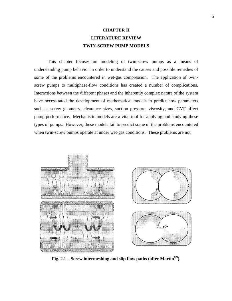
Fig. 2.1 – Screw intermeshing and slip flow paths (after Martin8,9).
6
predicted by the current pump models because they are based in part on assumptions
known to be invalid at high GVF. Currently, no twin-screw pump models exist that were
designed specifically with wet-gas compression in mind.
All current twin-screw pump models are based around the modeling of backflow
through the pump. Since the two screws of a pump do not touch, flow paths exist
through the small gaps formed. The pressure differential between the discharge and
suction sides of the pump causes backflow to occur. Backflow within the pump, also
known as slip flow, is a key factor in the operation of twin-screw pump since it is this slip
flow that seals and compresses the gas phase in each chamber. Most researchers have
therefore based their modeling efforts on understanding slip flow. Fig. 2.1, above,
illustrates the flow paths formed by the intermeshing screws. This chapter will attempt to
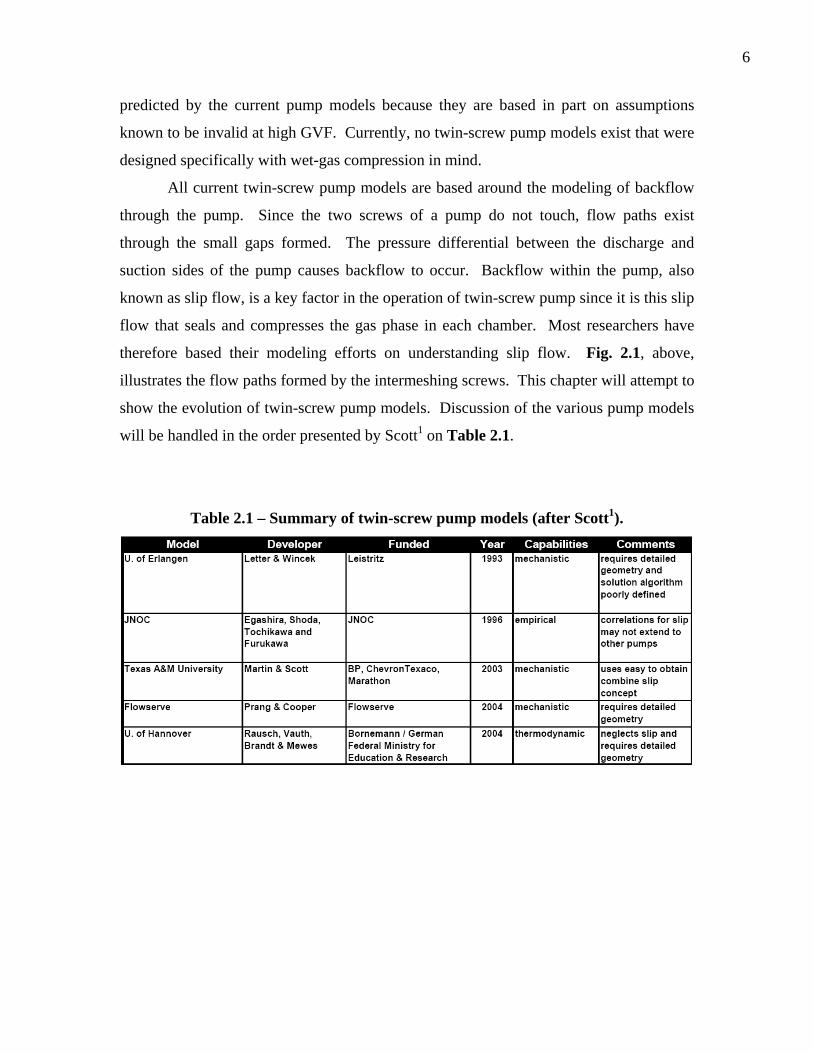
show the evolution of twin-screw pump models. Discussion of the various pump models
will be handled in the order presented by Scott1 on Table 2.1.
Table 2.1 – Summary of twin-screw pump models (after Scott1).
7
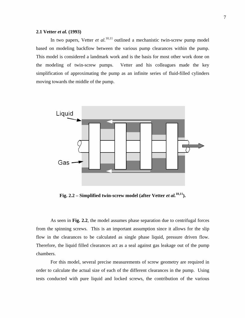
2.1 Vetter et al. (1993)
In two papers, Vetter et al.10,11 outlined a mechanistic twin-screw pump model
based on modeling backflow between the various pump clearances within the pump.
This model is considered a landmark work and is the basis for most other work done on
the modeling of twin-screw pumps. Vetter and his colleagues made the key
simplification of approximating the pump as an infinite series of fluid-filled cylinders
moving towards the middle of the pump.
Fig. 2.2 – Simplified twin-screw model (after Vetter et al.10,11).
As seen in Fig. 2.2, the model assumes phase separation due to centrifugal forces
from the spinning screws. This is an important assumption since it allows for the slip
flow in the clearances to be calculated as single phase liquid, pressure driven flow.
Therefore, the liquid filled clearances act as a seal against gas leakage out of the pump
chambers.
For this model, several precise measurements of screw geometry are required in
order to calculate the actual size of each of the different clearances in the pump. Using
tests conducted with pure liquid and locked screws, the contribution of the various
8
clearances were measured. The circumferential gap between the screw and the pump
casing was found to contribute the most to internal slip flow, accounting for
approximately 80% of the total.
The slip flow itself behaves like a piston, compressing the gas as it enters the
previous chamber. This gas compression process is assumed to be isothermal up to 96%
GVF, although no non-isothermal solution is given for GVF above this limit. The
assumption of liquid sealing in the clearances is recognized as a simplification and does
not reflect real conditions at high GVF.
In their second paper, Vetter et al. recognize that the assumption of liquid filled
clearances is not valid for GVF above 85%. They propose equations for adjusting the
fluid density and viscosity to reflect effect of gas and liquid mixture flowing through the
clearances are presented. The developed model was validated by running water-air
mixtures through a test pump.
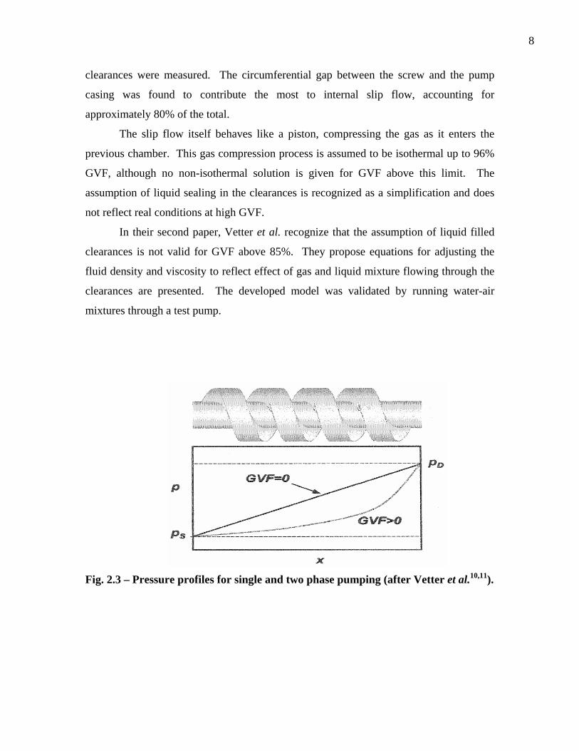
Fig. 2.3 – Pressure profiles for single and two phase pumping (after Vetter et al.10,11).

9
An interesting observation made was the shape of the pressure profiles along the
screw of the pump. As shown in Fig. 2.3, during single-phase flow the pressure profile is
linear. This means that each chamber of the pump is contributing equally to the overall
pressure boost provided by the pump. However for two-phase flow, the pressure profile
is no longer linear. As GVF increases, the compression occurring becomes more
concentrated in the chambers closer to the discharge.
Vetter et al.10,11 also discussed spindle shaft deformation resulting from
differential pressure differences along the shaft. According to them, the degree of shaft
deformation or deflection is independent of whether the pump is operating under single-
phase or two-phase conditions. Shaft deformation or deflection is an important feature
that would be incorporated into future models.
2.2 Egashira et al. (1996)
Egashira et al.12 took an empirical approach to modeling backflow in twin-screw
pumps. Using experimental data, they proposed an equation to calculate the pressure
profile along the screw.
1i s
d s t
p p ip p n
γ⎛ ⎞ ⎛−
=⎜ ⎟ ⎜− +⎝ ⎠ ⎝
⎞⎟⎠
(2.1)
This equation is a curve fit based on the parameter γ, which is adjusted to fit
experimental data. This curve fit is based on a single test pump so it may not be
applicable to other pump designs. Egashira et al.12 also identified the various pump
clearances through which slip flow occurs and showed that the amount of slip flow is
mainly a function of differential pressure, GVF, and shaft rotational speed.
Experimental data provided by Egashira et al.12 also confirms earlier experiments
about the nature of the pressure profile along the pump screws. As GVF increases the
pressure profile in the pump becomes more and more nonlinear. They also note that the
profile becomes steeper as of the pump speed and multiphase fluid compressibility
increase. The experiments conducted used water and air as test fluids.
A unique feature of the work described by Egashira et al.12 is their description of
possible backflow flow patterns. They describe three different patterns detailing the type
of flow, either pure water or an air and water mixture, in each of the four clearances they
10
define. The first pattern consists of pure water flow in the circumferential clearance
because of phase separation from centrifugal forces with a multiphase mixture in each of
the internal clearances. The second and third patterns are pure water or air and water
mixtures in all clearances, respectively.
2.3 Martin and Scott (2003)
The Martin and Scott8,9 model was developed to meet the need for a twin-screw
pump model for petroleum engineers. To properly design a twin-screw pump into a
production system, a complete set of pump tables is required. Though these tables can
sometimes be obtained from the pump manufacturer, an independent tool for predicting
pump performance was still needed. Previous models required detailed measurements of
screw geometry in order to calculate the size of the clearances. However, pump
manufacturers are usually unwilling to disclose these measurements since they are
regarded as trade secrets. To get around this limitation, Martin and Scott8,9 introduced a
system for calculating an effective clearance size based on pure-water performance data
using linear regression.
Martin and Scott8,9 were also the first to validate their pump model for liquids
with high viscosity using guar gel. Higher viscosity was observed to decrease slip rate.
The Martin and Scott8,9 model was also the first model to be confirmed to work with
different pump designs. Experiments were conducted with two different pumps and data
from two others was matched successfully.
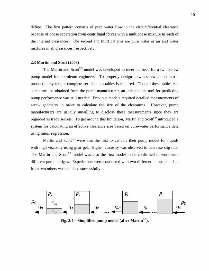
Fig. 2.4 – Simplified pump model (after Martin8,9).

11
A key component of this model is the gas compression module. As shown in Fig.
2.4, the pump is modeled as a series of independent chambers that are connected by slip
flow from one chamber to the previous chamber. The slip flow moves in the opposite
direction of the chambers as they are translated through the pump. This is similar to the
Vetter et al.10,11 model.
A set of moving control volumes is defined around each chamber, Fig. 2.4, which
allows for a set of equations to be written defining the pump behavior.
( )
( )
11 0
1
1 21 2 1
2 1
1 0
1 0
ss
s
p ZV q qp Z
p ZV q qp Z
⎛ ⎞⋅ t
t
⋅ − + − ⋅Δ =⎜ ⎟⋅⎝ ⎠⎛ ⎞⋅⋅ − + − ⋅Δ =⎜ ⎟⋅⎝ ⎠
M (2.2)
( )11 1
1
1 0i ii i i
i i
p ZV q qp Z
−− −
−
⎛ ⎞⋅⋅ − + − ⋅Δ⎜ ⎟⋅⎝ ⎠
t =
M
( )11 1
1
1 0n Dn n n
D n
p ZV q qp Z
−− −
−
⎛ ⎞⋅⋅ − + − ⋅Δ⎜ ⎟⋅⎝ ⎠
t =
In this system of equations the volumes, V, and the slip flow rates, q, are all
functions of pressure. Therefore, the pressure in each chamber must be solved
simultaneously. The Martin and Scott model utilized a Newton-Raphson algorithm to
solve for these pressures. Total slip flow through the entire pump and therefore the
pumping rate can then be calculated.

12
2.4 Cooper & Prang (2004)
Cooper & Prang13 proposed a twin-screw pump model based on similar methods
to previous models. However, Cooper & Prang13 clearly stated the assumptions made to
make a volumetric slip flow model possible. Two of the main assumptions are:
1. Complete liquid sealing in the clearances.
2. Liquid in the pump sufficient to carry away any heat generated so that the
pump is considered an isothermal system.
Cooper & Prang13 acknowledge that the assumption of liquid seals is invalid but
necessary. They too noted that at high GVF, the amount of gas compression occurring
becomes concentrated towards the discharge side of the pump. This imbalance causes a
severe pressure differential across the pump screws that may cause some vibration
problems observed in field operations. The source of these vibrations may be spatial
variation of the clearances, also termed spindle shaft deflection by other authors, caused
by the differential pressure causing the screw to come into contact with the pump casing.
Additionally, shaft deflection can dramatically change the shape of the circumferential
clearance leading to increased slip flow, especially in the laminar flow regime.
Cooper & Prang13 also discussed the effect of viscous heating on liquid viscosity.
They were able to validate their model for pure liquid high viscosity flow as well as high
GVF multiphase flow. Cooper & Prang13 observed increased volumetric efficiency with
the pump operating with higher viscosity liquids. Therefore, they note that changes in
operating conditions over time that may result in a decrease in liquid viscosity could
dramatically reduce twin-screw pump efficiency. This supports the need for better pump
models since for engineers to properly design a pump for the entire life of a well, pump
performance must be known for a variety of possible field conditions.

13
2.5 University of Hannover (2004)
In a paper from the University of Hannover, Rausch et al.14 approached the
modeling problem by combining a mass balance with an energy balance. For the first
time, the system was considered adiabatic instead of isothermal. Though it was known
that heat was generated in the pump from compression and viscous effects, it was always
assumed as a simplification that there was enough fluid in the pump to carry away most
of the heat. However, while the authors again acknowledge that the fluid in the
clearances may not be completely liquid, they are still forced to make this assumption.
The authors suggest that adoption of multiphase slip flow model is necessary to expand
model validity to wet-gas conditions. The model also considered internal recirculation of
liquid which is a design feature of some pumps.
Instead of a series of fluid filled cylinders as described in previous models, this
thermodynamic model describes twin-screw pump operation as two main components:
1. Individual chambers are modeled as moving volumes of mass and energy.
2. The gaps or clearances are streams where mass and energy are interchanged
between the chambers.
Therefore the pump is modeled as a series of mass and energy balances over a
moving control volume. Two different mass balances are proposed, one for the inlet
chamber, termed the first open chamber, and one for the closed chambers. The
conditions at which the fluid first enters the pump and the “filling process” it causes
necessitate the need for a different set of equations at the inlet.
Energy balances over each closed chamber are made assuming adiabatic
conditions and neglecting the kinetic energy of the slip flows and wall friction. This
allows for accurate calculations of the temperature in each chamber under non-isothermal
conditions. The energy balance given was made for constant volume chambers, although
the authors briefly mentioned the effect of progressive pitch screws. Having screws with
a progressive pitch would result in smaller chamber volumes and what the authors termed
a “built in compression”.
14
2.6 Model Comparisons and Thermal Issues
The Vetter, Cooper & Prang, and Hannover models were designed for use by
pump designers. As such, they require many different measurements of pump clearances
which may not always be available. As an alternative, Martin created a new twin-screw
pump model designed for use by petroleum engineers. The regression analysis used to
calculate effective pump clearances from pump performance data and is much more user
friendly while maintaining acceptable accuracy of prediction. Because of these factors,
the Martin model will be used for this research.
Singh6,7 examined temperature increases within twin-screw pumps during periods
of high GVF. He concluded that the assumption of an isothermal pump system is invalid
at GVF above 94%. From experimental data, Singh developed a thermodynamic model
that predicts temperature rise in twin-screw pumps at high GVF conditions. Toma15 has
presented field cases in which thermal effects such as flash boiling are the main cause for
destructive vibrations in the pump. Flash boiling results from the superheating of small
liquid droplets which fall into the gas phase. This directly refutes the assumption of an
isothermal system. Toma also showed evidence that in some cases pump volumetric
efficiency can exceed one.
The high pressure differentials observed across the screw during high GVF can
cause severe deflection of the screw shafts. Though all the pump models mentioned
above accounted for some deflection, whether or not the deflection is severe enough to
cause the screws to touch is unknown but may account for some of the vibrations and loss
of efficiency observed.

15
CHAPTER III
METHODS FOR WET-GAS COMPRESSION
This chapter focuses on methods for producing wet gas. Starting with
conventional techniques and moving on to new developments for wet-gas compression
with twin-screw pumps, the issues and solutions to the unique problems encountered with
wet-gas are explained. The two methods for improving twin-screw pump performance
proposed by Singh6,7 and investigated in this thesis are also presented. To understand the
methods presented, the concept of volumetric efficiency must first be defined.
3.1 Volumetric Efficiency
According to Martin8,9, the maximum theoretical flow rate, qTH, of a twin-screw
pump is simply a function of the pump’s displacement per revolution, D, and the pump
rotational speed, N. Pump displacement is dictated by screw geometry.
thq D N= ⋅ (3.1)
Although slip flow, qslip, through the pump creates a seal and compresses the gas
under two-phase conditions, it nevertheless subtracts from the theoretical flow rate.
Therefore the actual flow rate, q, is:
TH slipq q q= − (3.2)
Since the slip flow is a pressure driven flow through the internal clearances, as
differential pressure across the pump increases, slip flow will increase resulting in a drop
in actual flow rate. It is useful to define the volumetric efficiency, ηv, of the twin-screw
pump as:
TH slipv
TH TH
q qqq q
η−
= = (3.3)
From this definition we can see that any method of increasing the total flow rate
through the pump at given pump speed will improve volumetric efficiency.

16
3.2 Conventional Methods
The traditional method of boosting the pressure of a wet-gas stream is to use a
series of scrubbers and separators to create individual liquid and gas flow lines. The
liquid stream is then boosted using single-phase liquid pumps, while the gas stream is
compressed using dry-gas compressors. Fig. 3.1 and Fig. 3.2 illustrate the reduction in
process equipment possible by switching to a multiphase system to produce heavy oil and
annulus gas in a cyclic steam-flood application. An interesting feature of a multiphase
system is the ability to conserve system heat, preserving the mobility of the extremely
viscous bitumen.
Fig. 3.1 – Conventional production process flow diagram(after Dick and Speirs5).
17
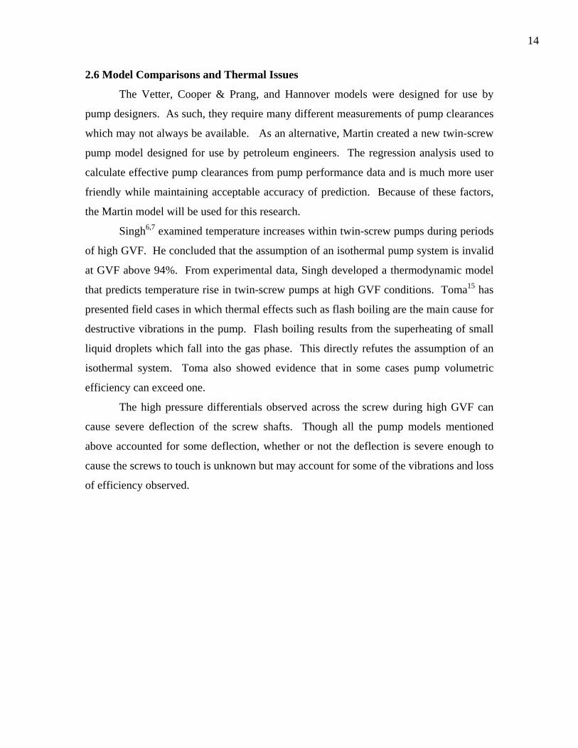
Fig. 3.2 – Multiphase production process flow diagram (after Dick and Speirs5).
3.3 Digressive Screws
A new development for improving twin-screw pump efficiency at high GVF is a
new generation of screws for high GVF operations introduced by Bornemann. These
“digressive” screws feature varying pitch along the screw, resulting in smaller and
smaller chamber volumes as the fluid approaches the discharge of the pump.2
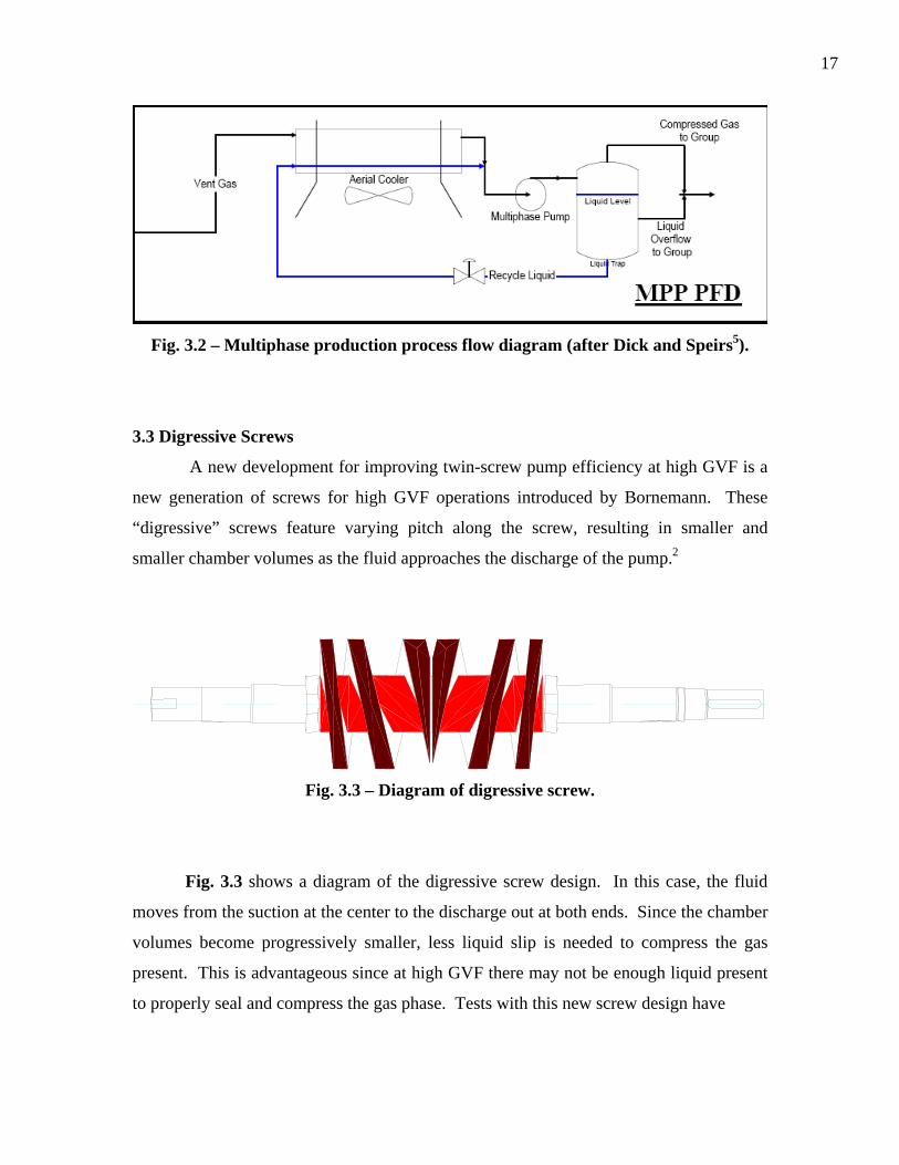
Fig. 3.3 – Diagram of digressive screw.
Fig. 3.3 shows a diagram of the digressive screw design. In this case, the fluid
moves from the suction at the center to the discharge out at both ends. Since the chamber
volumes become progressively smaller, less liquid slip is needed to compress the gas
present. This is advantageous since at high GVF there may not be enough liquid present
to properly seal and compress the gas phase. Tests with this new screw design have

18
demonstrated a significant increase in flow capacity, efficiency, and a decrease in power
consumption over conventional screw designs at high GVF, Fig. 3.4.
Fig. 3.4 – Digressive screw test results (after Rohlfing and Muller-Link16).
Though the results are promising, methods of achieving this improvement without
the need to replace screw sets have been proposed. Even with these new screws, a GVF
of 95% is recommended to ensure that there is sufficient liquid in the pump.
3.4 High Viscosity Fluid Circulation
Singh6,7, Martin8,9, and Cooper & Prang13 have all presented evidence that shows
that increasing the viscosity of the liquid phase reduces slip flow leading to higher
volumetric efficiency, Fig. 3.5.
Martin suggested that the lower slip flow with higher viscosity fluids would
decrease the amount of volume taken up by slip liquid in the suction end of the pump.
This would enable more fluid to be taken into the pump at high GVF conditions. Fig. 3.6
presents in an illustration of this concept.

19
Fig. 3.5 – Viscosity effects on liquid flow rate (after Martin8,9).
Singh therefore tested various liquid viscosities at high GVF all the way to 100%
on a Bornemann MW 6.5zk-37 twin-screw pump. The Bornemann pump was selected
because of the recirculation chamber integrated into its design which allows for more
liquid to be retained in the pump at high GVF. This recirculation chamber allows the
pump to maintain operation at 100% GVF for a short period of time.

20
Fig. 3.6 – Reduced slip allows for more gas flow (after Martin8,9).
Pump performance at 100%Gas_45Hz_for 1 & 9 CP liquid injection(providing the seal)
0
50
100
150
200
25
0
0 20 40 60 80 100 120 140 160
Differential Pressure, psia
Gas
Flo
w R
ate,
GPM
45Hz_100%Gas_09CP45Hz_100Gas_1CP FluidPoly. (45Hz_100%Gas_09CP)Poly. (45Hz_100Gas_1CP Fluid)
Fig. 3.7 – Gas flow rate versus differential pressure for different liquid viscosities,
pump speed 1350 RPM (after Singh6,7).
21
Pump performance at 100% Gas_25Hz_for1 & 9 CP liquid injection(providing the seal)
0
20
40
60
80
100
120
140
0 20 40 60 80 100 120 140
Differential Pressure, psia
Gas
Flo
wra
te, G
PM
25Hz_9CP25Hz_1CP Poly. (25Hz_1CP )
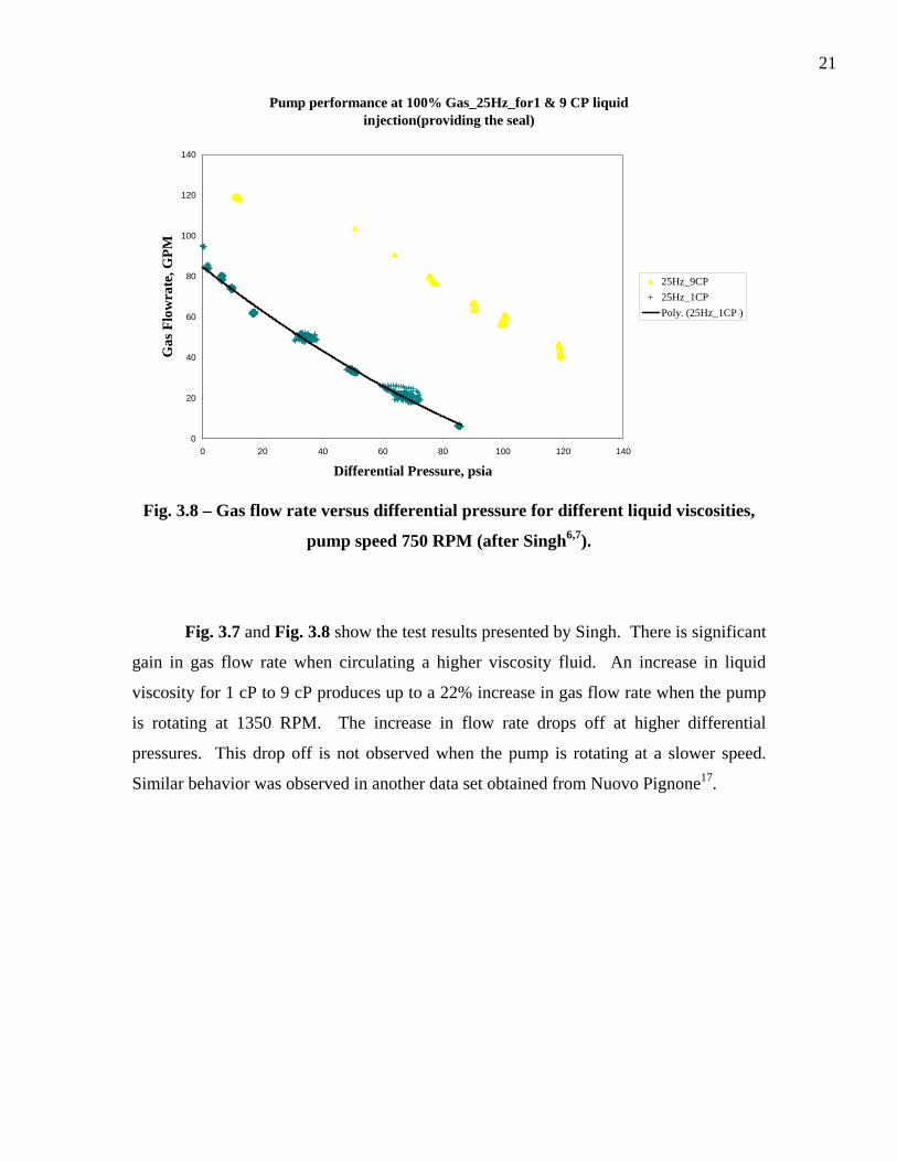
Fig. 3.8 – Gas flow rate versus differentia pressure for different liquid viscosities,
ig. 3.7 and Fig. 3.8 show the test results presented by Singh. There is significant
gain in
l
pump speed 750 RPM (after Singh6,7).
F
gas flow rate when circulating a higher viscosity fluid. An increase in liquid
viscosity for 1 cP to 9 cP produces up to a 22% increase in gas flow rate when the pump
is rotating at 1350 RPM. The increase in flow rate drops off at higher differential
pressures. This drop off is not observed when the pump is rotating at a slower speed.
Similar behavior was observed in another data set obtained from Nuovo Pignone17.
22
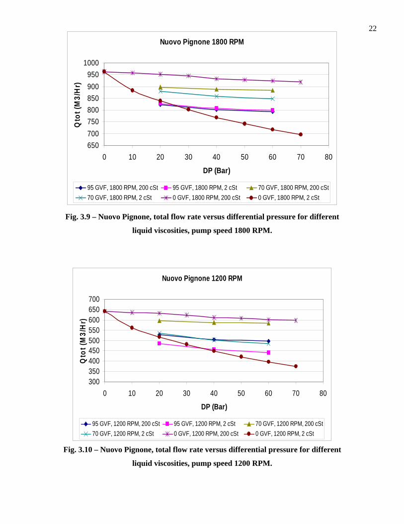
Fig. 3.9 – Nuovo Pignone, total flow rate versus differential pressure for different
Nuovo Pignone 1800 RPM
650700750800850900950000
0 10 20 30 40 50 60 70 80
DP (Bar)
Qto
t (M
3/H
r)
1
95 GVF, 1800 RPM, 200 cSt
liquid viscosities, pump speed 1800 RPM.
Fig. 3.10 – Nuovo Pignone, total flow rate versus differential pressure for different
liquid viscosities, pump speed 1200 RPM.
95 GVF, 1800 RPM, 2 cSt 70 GVF, 1800 RPM, 200 cSt70 GVF, 1800 RPM, 2 cSt 0 GVF, 1800 RPM, 200 cSt 0 GVF, 1800 RPM, 2 cSt
Nuovo Pignone 1200 RPM
300350400450500550600650700
0 10 20 30 40 50 60 70 80
DP (Bar)
Qto
t (M
3/H
r)
95 GVF, 1200 RPM, 200 cSt 95 GVF, 1200 RPM, 2 cSt 70 GVF, 1200 RPM, 200 cSt70 GVF, 1200 RPM, 2 cSt 0 GVF, 1200 RPM, 200 cSt 0 GVF, 1200 RPM, 2 cSt

23
Fig. 3.9 shows 2 and 200 cSt fluid at
a pump
the results of experiments conducted with a
speed of 1800 RPM. At a GVF of 95%, there is a slight decrease in total flow
rate with increasing viscosity. In Fig. 3.10, the pump speed is slower at 1200 RPM. In
that case, there is a large increase in total flow rate with increasing viscosity. Fig. 3.11
summarizes the differences.
-5
0
5
10
15
20
25
Pignone 1800 RPM Pignone 1200 RPM Singh - Bornemann 1350 RPM
% Im
prov
emen
t
Fig. 3.11 – Improvement in total flow rate with increased viscosity.
From the results of his experiments, Singh proposed a system where the viscosity
of the l
iquid phase would be artificially increased. Since liquid is already captured for re-
circulation to maintain a minimum GVF, an additive could be introduced to increase the
viscosity. Flow assurance fluids which are often used to prevent hydrate formation or
corrosion could also provide another source fluid for increasing the viscosity.
24
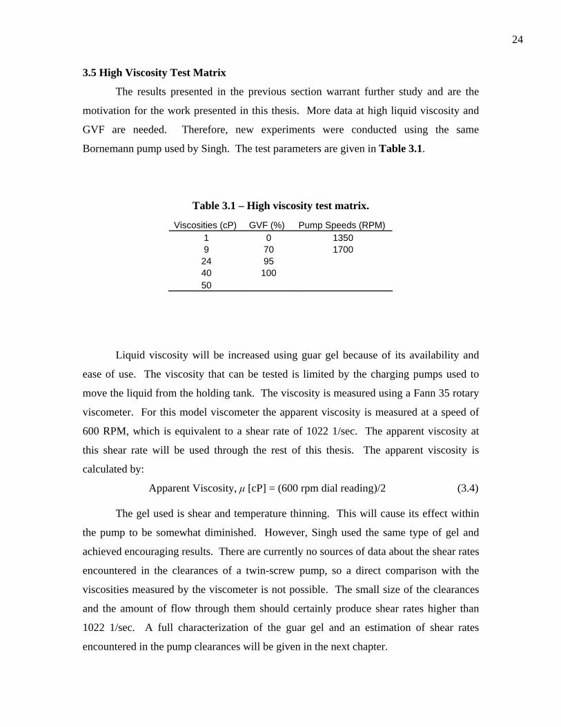
3.5 High Viscosity Test Matrix
he previous section warrant further study and are the
motiva
Table 3.1 – High viscosity test matrix.
Visc M)
The results presented in t
tion for the work presented in this thesis. More data at high liquid viscosity and
GVF are needed. Therefore, new experiments were conducted using the same
Bornemann pump used by Singh. The test parameters are given in Table 3.1.
osities (cP) GVF (%) Pump Speeds (RP1 0 1350 9 70 1700 24 95 40 100 50
iquid viscosity will be increased using guar gel because of its availability and
ease of
Apparent Viscosity, μ [cP] = (600 rpm dial reading)/2 (3.4)
he ge
the pum
L
use. The viscosity that can be tested is limited by the charging pumps used to
move the liquid from the holding tank. The viscosity is measured using a Fann 35 rotary
viscometer. For this model viscometer the apparent viscosity is measured at a speed of
600 RPM, which is equivalent to a shear rate of 1022 1/sec. The apparent viscosity at
this shear rate will be used through the rest of this thesis. The apparent viscosity is
calculated by:
T l used is shear and temperature thinning. This will cause its effect within
p to be somewhat diminished. However, Singh used the same type of gel and
achieved encouraging results. There are currently no sources of data about the shear rates
encountered in the clearances of a twin-screw pump, so a direct comparison with the
viscosities measured by the viscometer is not possible. The small size of the clearances
and the amount of flow through them should certainly produce shear rates higher than
1022 1/sec. A full characterization of the guar gel and an estimation of shear rates
encountered in the pump clearances will be given in the next chapter.

25
3.6 Through-Casing Injection
Singh also proposed injecting liquid through the pump casing, directly into the
ump c
Fig. 3.12 – Theoretical pressure profile with through-casing injection.
ig. 3.12 shows the type of pressure profile that is thought to be possible using
through
p hambers. This injected liquid would help maintain the seal around the chambers
and could facilitate control of the internal pressure profile. By increasing the amount of
liquid in a specific chamber in the pump, we could increase the pressure in that chamber
and allow an operator to create a more favorable linear pressure profile. This is similar to
the operating concept of the digressive screw design, but instead of decreasing the
chamber volume mechanically, it will be attempted hydro dynamically
Distance A ong Screw
Pres
sure
Diff
eren
tial
F
-casing injection. The compression ratio of the chambers closer to the discharge
is reduced and the chambers near the suction side of the pump now contribute to the
overall pressure boost. By eliminating sudden changes in pressure within the pump, it is
thought that some of the vibration issues encountered can be eliminated. This method
may be able to increase the total boosting capacity of the pump since the pressures in the
l
GVF = 0
GVF > 0
Distance A ong Screw
Pres
sure
Diff
eren
tial
l
GVF = 0
GVF > 0

26
pump chambers will be increased. Since this method requires significant modifications
challen
Fig. 3.13 – Diagram of injection timing problem.
to an expensive piece of machinery, it will be examined only theoretically in this thesis.
The implementation through-casing injection presents many mechanical
ges. Injecting fluid into a chamber rotating in excess of 1800 RPM will be
difficult. At any given time when injecting at a single point along the pump casing, the
outer portion of the screw may block the injection port, Fig. 3.13. A timing system or a
wider slot for injection must be developed before any field trials may be conducted.

27
CHAPTER IV
EXPERIMENTAL FACILITY
This chapter is a description of the multiphase field laboratory at the Texas
A&M Riverside campus. This facility was used for all the experiments described in this
thesis. The remote location of the Riverside campus, approximately 15 miles from
College Station, allows for the testing of real pieces of oilfield equipment that would
not be possible in a normal research setting.
Riverside is a field-scale experimental test facility which features two full-size
twin-screw multiphase pumps. The smaller of the two pumps is a Bornemann MW-
6.5zk-37. This pump has a capacity of 10,000 bbl/day with a maximum pressure boost
of 250 psig. An important feature of this pump is its internal recirculation chamber.
This allows for some of the liquid at the discharge to be moved back to the suction end
of the pump. Fig. 4.1 shows a side view of the Bornemann pump. The discharge from
the pump is upwards to help retain liquid. The recirculation chamber can be seen
branching off from the discharge.

28
Fig. 4.1 – Bornemann MW-6.5zk-37 twin-screw pump with internal recirculation
chamber.
Fig. 4.2 – Rendition of Riverside test facility (Martin8,9).
29
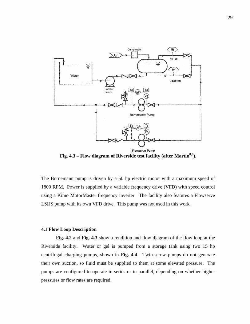
Fig. 4.3 – Flow diagram of Riverside test facility (after Martin8,9).
The Bornemann pump is driven by a 50 hp electric motor with a maximum speed of
1800 RPM. Power is supplied by a variable frequency drive (VFD) with speed control
using a Kimo MotorMaster frequency inverter. The facility also features a Flowserve
LSIJS pump with its own VFD drive. This pump was not used in this work.
4.1 Flow Loop Description
Fig. 4.2 and Fig. 4.3 show a rendition and flow diagram of the flow loop at the
Riverside facility. Water or gel is pumped from a storage tank using two 15 hp
centrifugal charging pumps, shown in Fig. 4.4. Twin-screw pumps do not generate
their own suction, so fluid must be supplied to them at some elevated pressure. The
pumps are configured to operate in series or in parallel, depending on whether higher
pressures or flow rates are required.

30
Fig. 4.4 – Centrifugal charging pumps.
Air from a 185 CFM compressor is stored in a pressure vessel, Fig. 4.5. For
testing at high GVF, the liquid is also pumped into this vessel. Doing this allows the
pressure of each phase to equalize and greatly reduces any slugging effects from phase
mixing. Liquid is then allowed to flow from the bottom of the vessel while the air
comes from the top.

31
Fig. 4.5 – Pressure equalization vessel.
The separate air and liquid lines are then passed into a metering section. Mass
flow rates are measured using MicroMotion Elite series Coriolis meters. A three inch
meter, model CMF300M355NUR, is used for the liquid while a one inch meter, Model
CMF100M329NU, is used for the gas. These types of meters are highly accurate with
errors of +/- 0.10% for liquid flow rates and +/- 0.50% for gas flow rates. Valves at the
metering section allow the flow rate of liquid and gas sent to the twin-screw pump to be
adjusted. The GVF of the flow stream sent to the pump is adjusted in this way. After
metering, the liquid and air lines are combined at a mixing tee. The metering section
and mixing tee are shown in Fig. 4.6.

32
The combined flow stream then moves through either a six or four inch flow line
to the Bornemann pump. Two Weed 201 Direct Immersion RTDs provide temperature
measurements at both the suction and discharge ends of the pump. These devices have
an accuracy of +/- 0.54oF. Rosemount model 3051 pressure transducers are used to
measure the suction and discharge pressures. These pressure sensors have an accuracy
of +/- 0.075%.
Fig. 4.6 – Metering section and mixing tee.
33
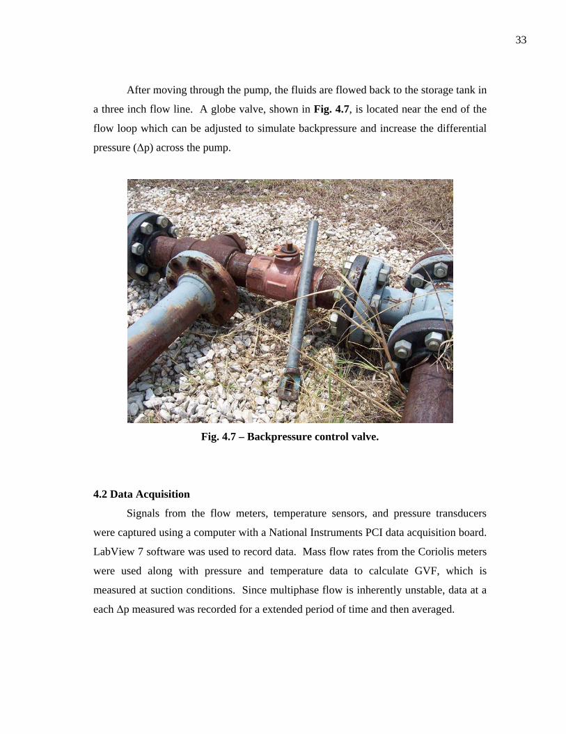
After moving through the pump, the fluids are flowed back to the storage tank in
a three inch flow line. A globe valve, shown in Fig. 4.7, is located near the end of the
flow loop which can be adjusted to simulate backpressure and increase the differential
pressure (Δp) across the pump.
Fig. 4.7 – Backpressure control valve.
4.2 Data Acquisition
Signals from the flow meters, temperature sensors, and pressure transducers
were captured using a computer with a National Instruments PCI data acquisition board.
LabView 7 software was used to record data. Mass flow rates from the Coriolis meters
were used along with pressure and temperature data to calculate GVF, which is
measured at suction conditions. Since multiphase flow is inherently unstable, data at a
each Δp measured was recorded for a extended period of time and then averaged.

34
4.3 Viscosity Control
Guar gel is mixed as a liquid concentrate in the storage tank at various
concentrations corresponding with the viscosity desired. A small five horsepower
centrifugal pump is used to roll the tank, ensuring thorough mixing. Fig. 4.8 shows
the relationship between gel concentration (lb/gal) and viscosity (cP) measured at four
different shear rates.
0
50
100
150
200
250
300
350
0 10 20 30 40 50 60 70 8
Gel Concentration (lb/1000 gal)
Visc
osity
(cP)
0
1022 1/sec 511 1/sec 341 1/ sec 170 1/sec
Fig. 4.8 – Gel concentration versus viscosity at different shear rates.
Viscosity was measured using a Fann 35 rotary viscometer with the four shear
rates presented in Fig. 4.8 corresponding to viscometer speeds of 600, 300, 200, and
100 RPM, respectively. Samples were taken out of the storage tank periodically and
tested to ensure constant viscosity and gel concentration. The gel is a non-Newtonian
pseudoplastic fluid. The viscosity of the fluid, μ, can represented as a function of shear
rate, γ, in the form of:

35
( ) 1nKμ γ −= (4.1)
In this equation K is the flow consistency index while n is the flow behavior index. A
Newtonian fluid has an n value of one. To determine n for the guar gel used in the
experiments presented in this thesis, shear rate data obtained from a viscometer is
plotted versus apparent viscosity for each of the different gel concentrations, Fig. 4.9.
0500
1000150020002500300035004000
0 200 400 600 800 1000
Shear Rate (1/sec)
App
aren
t Vis
cosi
ty (c
P)
20 lb 40 lb 60 lb 80 lbPower (80 lb) Power (60 lb) Power (40 lb) Power (20 lb)
Fig. 4.9 – Apparent viscosity (cP) versus shear rate (sec-1) for different gel
concentrations.
It is clear from Fig. 4.9 that this gel exhibits power law behavior. Curve fits on
data from viscometer measurements are performed to calculate K and n, Table 4.1
summarizes the results. As expected, the gel becomes more non-Newtonian as gel
concentration increases.

36
Table 4.1 – Values of flow consistency index, K, and flow behavior index, n,
for gels of different concentrations.
Gel Concentration (lb/1000 gal) Flow Consistency Index, K Flow Behavior Index, n 20 88.8 0.720 40 1295.3 0.466 60 4321.3 0.361 80 12363.0 0.284
The shear thinning behavior observed in Fig. 4.9 presents the problem of
decreased effectiveness of the gel in the high shear clearances in the pump. An
estimation of the shear rates encountered within a twin-screw pump can be made by
approximating the flow through the circumferential clearance, the gap between the outer
part of the screw and the pump casing, as single phase liquid flow through a thin
channel. Using measurements of the screw diameter and circumferential clearance, the
area of the clearance can be calculated. Martin6 gives values for the external screw
diameter, Dc, and the effective circumferential clearance, for the Bornemann pump.
Using the shape of the circumferential clearance presented in Fig. 2.1, a circumferential
area, Ac, in ft2 consisting of two circular areas can be calculated as:
( )( )2 22
144c c c
c
D c DA
π ⋅ + −= (4.2)
The screw measurements and the calculated area are given below in Table 4.2.
Table 4.2 – Clearance measurements and calculated area.
Dc (in.) cc (in.) Ac (ft2) 5.24 0.0109 0.004989

37
Using slip flow rates calculated from the Martin model, the velocity of the fluid
in the clearance can be calculated. The slip flow rates given by the model are in both
directions so it is divided by two. Addionally, Vetter et. al.10,11 determined that 80% of
the slip flow passes through the circumferential clearance.
0.8
0.0022282
slip
c
qv
A⎛ ⎞
= ⋅⎜⎝ ⎠
⎟ (4.3)
Assuming no slip flow at the wall, the shear rate can be calculated by:
12
c
vc
γ = (4.4)
Table 4.3 summarizes the shear rates encountered in the circumferential
clearance of the Bornemann pump for different differential pressures and slip flow
rates. The large amount of slip flow and the extremely narrow clearances contribute to
estimated shear rates that are much higher than those observed in the viscometer.
Table 4.3 – Calculated shear rates at different slip flow rates.
qslip (GPM) v (ft/sec) γ (sec-1) ΔP = 150 psi 169.26 30.23 33283.90 ΔP = 100 psi 130.82 23.37 25724.39 ΔP = 50 psi 91.08 16.27 17910.98
Extrapolated viscosities from the data shown in Fig. 4.9 at the calculated shear
rates for different concentration gels are given below in Table 4.4. Eq. 4.1 was used
with the values of K and n from Table 4.1.
38
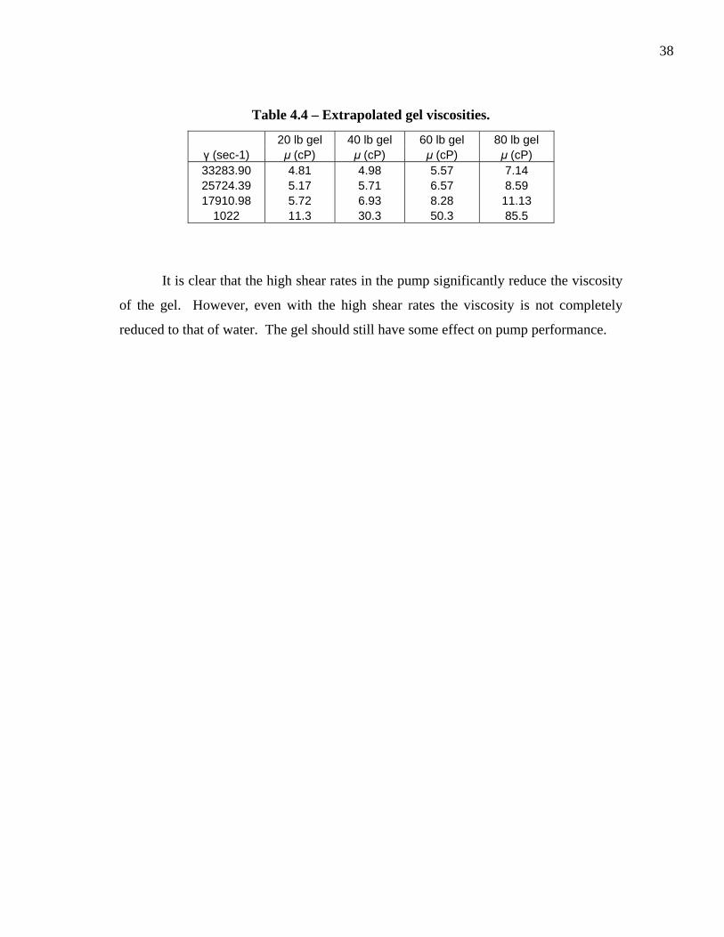
Table 4.4 – Extrapolated gel viscosities.
20 lb gel 40 lb gel 60 lb gel 80 lb gel γ (sec-1) μ (cP) μ (cP) μ (cP) μ (cP) 33283.90 4.81 4.98 5.57 7.14 25724.39 5.17 5.71 6.57 8.59 17910.98 5.72 6.93 8.28 11.13
1022 11.3 30.3 50.3 85.5
It is clear that the high shear rates in the pump significantly reduce the viscosity
of the gel. However, even with the high shear rates the viscosity is not completely
reduced to that of water. The gel should still have some effect on pump performance.

39
CHAPTER V
HIGH VISCOSITY CIRCULATION
This chapter presents the results and discussion of all work done on high viscosity
liquid circulation in twin-screw pumps at high GVF. Tests conducted with pure liquid
will be presented to demonstrate the effect of elevated viscosity on this type of pump.
The results of the extensive tests conducted under wet-gas conditions will then be shown
and compared to model predictions.
It is common to express pump flow rates at suction conditions. All flow rates
given in this chapter are at suctions conditions. Liquid flow rate is calculated by dividing
the mass flow rate (lb/min) by the liquid density (lb/gal) both values given by the Coriolis
meter.
.
l lq m lρ= × (5.1) Gas flow rates are calculated in a similar way except that the real gas law is used to
calculate the density at suction conditions. The gas in this case is assumed to be an ideal
gas.
.
g gq m gρ= × (5.2)
suctiong
suction
MpzRT
ρ = (5.3)
Total flow rate is simply the gas and liquid flow rates added together.
t lq q qg= + (5.4)

40
5.1 Pure Liquid Tests
Tests with pure liquid, 0% GVF, at various viscosities were conducted to quantify
the effect of increased viscosity on pump performance. Pump curves showing flow rate
in gallons per minute versus differential pressure (psi) across the pump are presented.
The full results of these tests are shown below in Fig. 5.1 and are similar to previously
published data. Viscosities reported were measured at a shear rate of 1022 sec-1.
0
50
100
150
200
250
0 50 100 150 200
Differential Pressure (psi)
Liqu
id F
low
Rat
e (G
PM)
1 cP, 1350 RPM 1 cP, 1700 RPM 9 cP, 1350 RPM9 cP, 1700 RPM 26 cP, 1350 RPM 26 cP, 1700 RPM40 cP, 1350 RPM 40 cp, 1700 RPM Poly. (1 cP, 1350 RPM)
Fig. 5.1 – Liquid flow rate (GPM) versus differential pressure (psi) for four
different viscosities and two pump speeds.
Higher differential pressure results in increased slip flow which in turn results in
lower flow rate through the pump. Therefore volumetric efficiency decreases with
increasing differential pressure. As expected, the higher pump speed produces higher
flow rates. Slip rate is known to be independent of pump speed. Therefore, volumetric
efficiency increases as pump increases, Fig. 5.2.
41
0%
10%
20%
30%
40%
50%
60%
70%
80%
90%
0 20 40 60 80 100 120 140 160 180 200
Differential Pressure (psi)
Volu
mes
tric
Effic
ienc
y
1700 RPM 1350 RPM Poly. (1350 RPM)
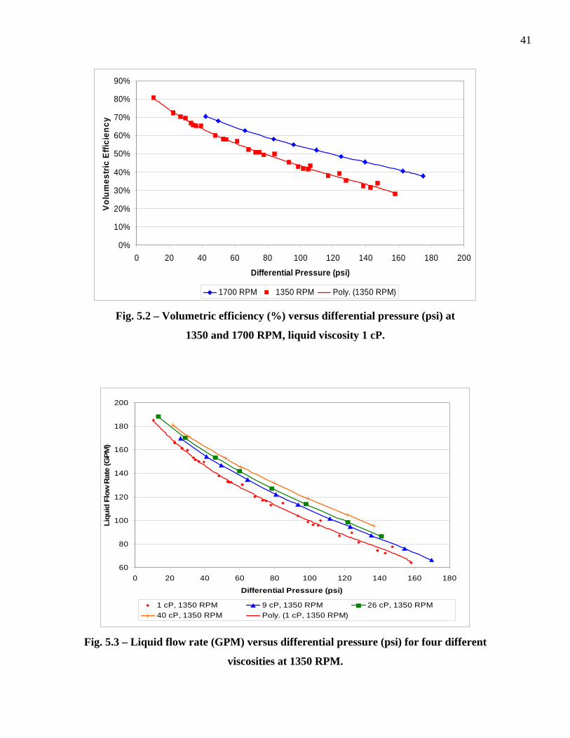
Fig. 5.2 – Volumetric efficiency (%) versus differential pressure (psi) at
1350 and 1700 RPM, liquid viscosity 1 cP.
60
80
100
120
140
160
180
200
0 20 40 60 80 100 120 140 160 180
Differential Pressure (psi)
Liqu
id F
low
Rat
e (G
PM)
1 cP, 1350 RPM 9 cP, 1350 RPM 26 cP, 1350 RPM40 cP, 1350 RPM Poly. (1 cP, 1350 RPM)
Fig. 5.3 – Liquid flow rate (GPM) versus differential pressure (psi) for four different
viscosities at 1350 RPM.
42
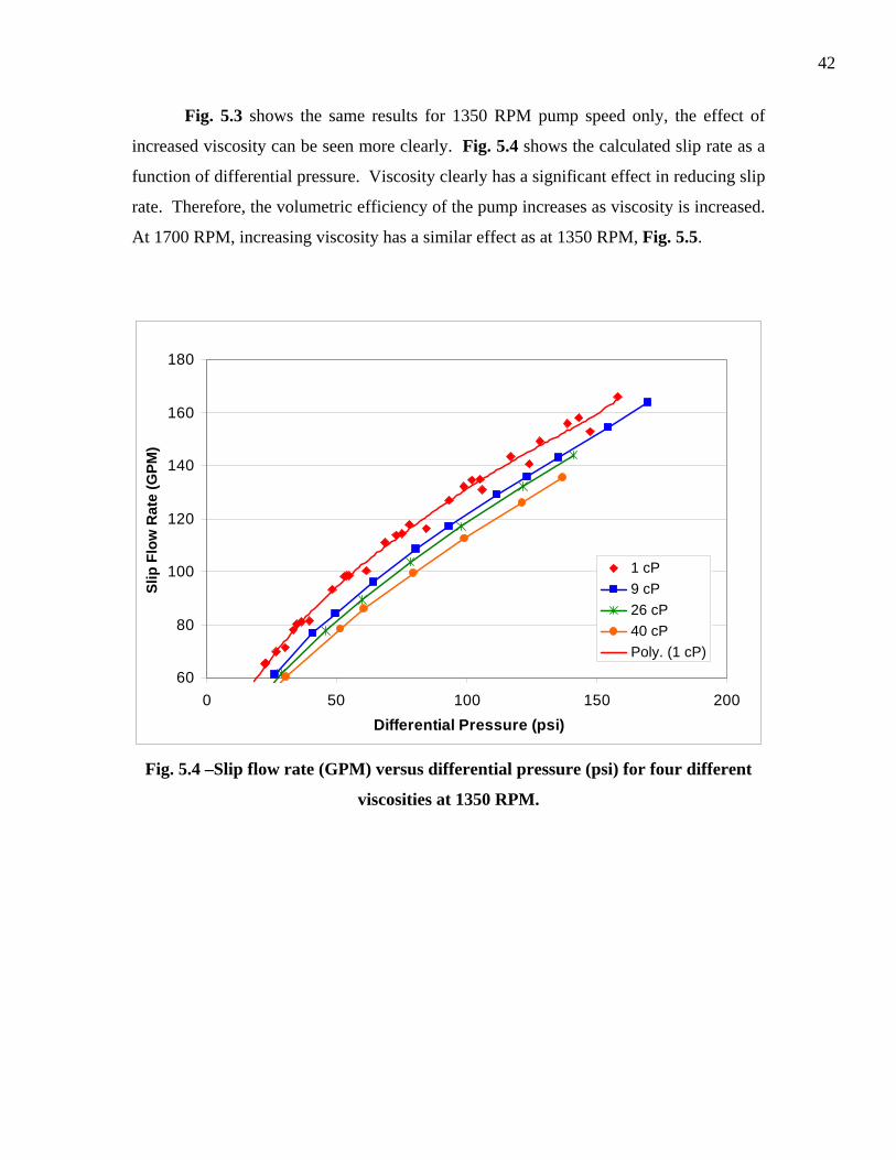
Fig. 5.3 shows the same results for 1350 RPM pump speed only, the effect of
increased viscosity can be seen more clearly. Fig. 5.4 shows the calculated slip rate as a
function of differential pressure. Viscosity clearly has a significant effect in reducing slip
rate. Therefore, the volumetric efficiency of the pump increases as viscosity is increased.
At 1700 RPM, increasing viscosity has a similar effect as at 1350 RPM, Fig. 5.5.
60
80
100
120
140
160
180
0 50 100 150 200Differential Pressure (psi)
Slip
Flo
w R
ate
(GPM
)
1 cP9 cP26 cP40 cPPoly. (1 cP)
Fig. 5.4 –Slip flow rate (GPM) versus differential pressure (psi) for four different
viscosities at 1350 RPM.

43
100
120
140
160
180
200
220
240
0 50 100 150 200
Differential Pressure (psi)
Liqu
id F
low
Rat
e (G
PM)
1 cP, 1700 RPM 9 cP, 1700 RPM26 cP, 1700 RPM 40 cP, 1700 RPM
Fig. 5.5 – Liquid flow rate (GPM) versus differential pressure (psi) for four different
viscosities at 1700 RPM.
5.2 100% GVF Tests
In attempt to reproduce the results of the experiments conducted by Singh6,7, tests
were conducted at 100% GVF using a 1 and 9 cP liquid. Pure liquid was flowed through
the pump for an extended period of time. The liquid flow was then cut-off and
compressed gas was then sent through the pump, leaving only the fluid left inside the
pump to maintain the seals and provide compression. To ensure that the results are
comparable, the same Bornemann twin-screw pump and gel used by Singh was used for
this set of tests.
44
0
20
40
60
80
100
120
140
160
180
200
0 20 40 60 80 100 120 140 160 180
Differential Pressure (psi)
Gas
Flo
w R
ate
(GPM
)1 cP9 cP
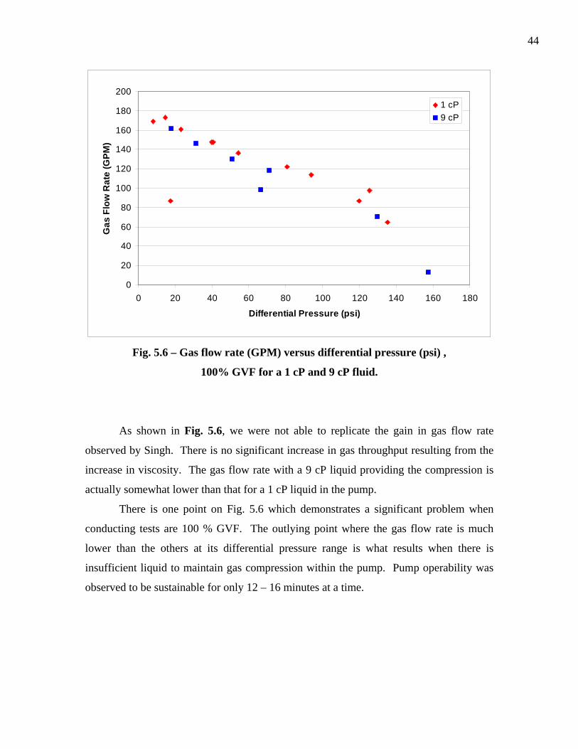
Fig. 5.6 – Gas flow rate (GPM) versus differential pressure (psi) ,
100% GVF for a 1 cP and 9 cP fluid.
As shown in Fig. 5.6, we were not able to replicate the gain in gas flow rate
observed by Singh. There is no significant increase in gas throughput resulting from the
increase in viscosity. The gas flow rate with a 9 cP liquid providing the compression is
actually somewhat lower than that for a 1 cP liquid in the pump.
There is one point on Fig. 5.6 which demonstrates a significant problem when
conducting tests are 100 % GVF. The outlying point where the gas flow rate is much
lower than the others at its differential pressure range is what results when there is
insufficient liquid to maintain gas compression within the pump. Pump operability was
observed to be sustainable for only 12 – 16 minutes at a time.

45
5.3 GVF Progression
The majority of tests were conducted at 0%, 70%, and 95% GVF. Because of the
inherent instability of testing at 100% GVF and since most pump installations are
maintained at a maximum GVF of 95% no further tests were conducted with pure gas.
Pump behavior under wet-gas conditions was evaluated at 95% GVF. Tests were
conducted at 70% GVF to provide comparison to a mostly gas but not wet-gas condition.
0
20
40
60
80
100
120
140
160
180
200
0 20 40 60 80 100 120 140 160 180 200
Differential Pressure (psi)
Tota
l Flo
w R
ate
(GPM
)
1 cP, 95 GVF 1 cP, 0 GVF 1 cP, 70 GVF
Fig. 5.7 – GVF progression, total flow rate (GPM) versus
differential pressure (psi), 1 cP fluid at 1350 RPM.

46
0
50
100
150
200
250
300
0 20 40 60 80 100 120 140 160 180 200
Differential Pressure (psi)
Tota
l Flo
w R
ate
(GPM
)
1 cP, 95 GVF 1 cP, 0 GVF 1 cP, 70 GVF
Fig. 5.8 – GVF progression, total flow rate (GPM) versus
differential pressure (psi), 1 cP fluid at 1700 RPM.
Figs 5.7 and Fig. 5.8 show pump curves at different GVF for 1350 and 1700 RPM
pump speeds, respectively. At 1350 RPM, there is a slight increase in total flow rate flow
and therefore a slight increase in volumetric efficiency. This is due to gas compression
enabling more gas to be taken into the pump. The effect at 1700 RPM is similar, but the
difference between 70 and 95% GVF is negligible with the 70% GVF slightly higher.
This suggests that there is a limit to the gas compression phenomena that is being reached
at the higher pump speed.

47
5.4 Speed Comparison
0
50
100
150
200
250
300
0 20 40 60 80 100 120 140 160 180 200
Differential Pressure (psi)
Tota
l Flo
w R
ate
(GPM
)
9 cP, 1350 RPM 24 cP, 1350 RPM 40 cP. 1350 RPM 50 cP, 1350 RPM 1 cP, 1350 RPM1 cP, 1700 RPM 9 cP, 1700 RPM 24 cP, 1700 RPM 40 cP, 1700 RPM 50 cP, 1700 RPM
Fig. 5.9 – Speed comparison, total flow rate (GPM) versus differential
pressure (psi), 95% GVF.
As speed increases total flow rate is expected to increase. This is confirmed by
the data presented in Fig. 5.9. Increase in flow rate is a constant offset from the lower to
higher speed. This provides further evidence that slip rate is independent of pump speed.
48
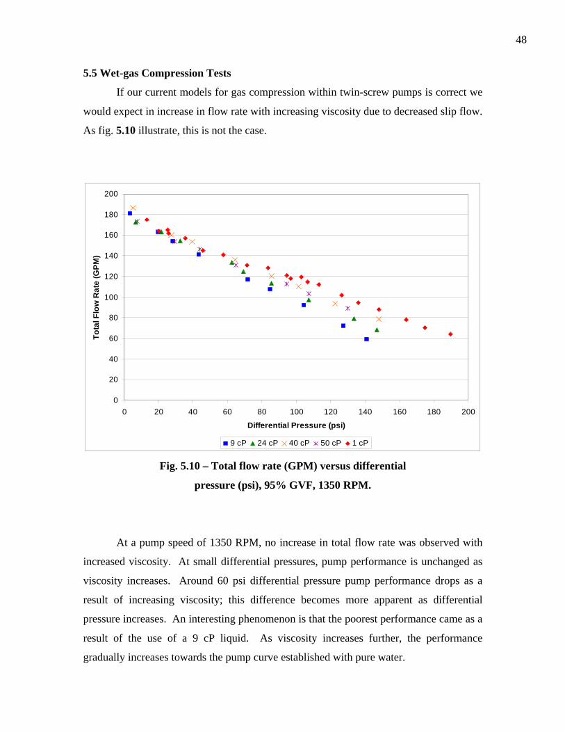
5.5 Wet-gas Compression Tests
If our current models for gas compression within twin-screw pumps is correct we
would expect in increase in flow rate with increasing viscosity due to decreased slip flow.
As fig. 5.10 illustrate, this is not the case.
0
20
40
60
80
100
120
140
160
180
200
0 20 40 60 80 100 120 140 160 180 200
Differential Pressure (psi)
Tota
l Flo
w R
ate
(GPM
)
9 cP 24 cP 40 cP 50 cP 1 cP Fig. 5.10 – Total flow rate (GPM) versus differential
pressure (psi), 95% GVF, 1350 RPM.
At a pump speed of 1350 RPM, no increase in total flow rate was observed with
increased viscosity. At small differential pressures, pump performance is unchanged as
viscosity increases. Around 60 psi differential pressure pump performance drops as a
result of increasing viscosity; this difference becomes more apparent as differential
pressure increases. An interesting phenomenon is that the poorest performance came as a
result of the use of a 9 cP liquid. As viscosity increases further, the performance
gradually increases towards the pump curve established with pure water.
49
100
120
140
160
180
200
220
240
40 60 80 100 120 140 160 180
Differential Pressure (psi)
Tota
l Flo
w R
ate
(GPM
)
1 cP 10 cP 26 cP 40 cP 50 cP
Fig. 5.11 – Total flow rate (GPM) versus differential
pressure (psi), 95% GVF, 1700 RPM.
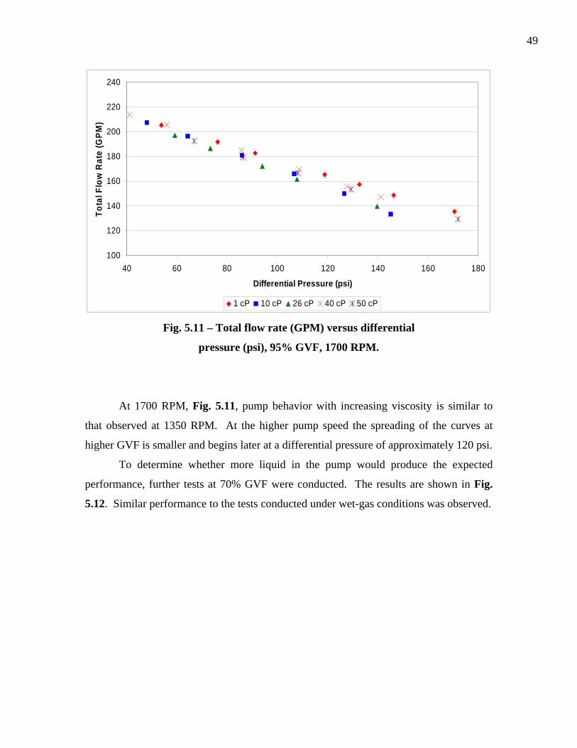
At 1700 RPM, Fig. 5.11, pump behavior with increasing viscosity is similar to
that observed at 1350 RPM. At the higher pump speed the spreading of the curves at
higher GVF is smaller and begins later at a differential pressure of approximately 120 psi.
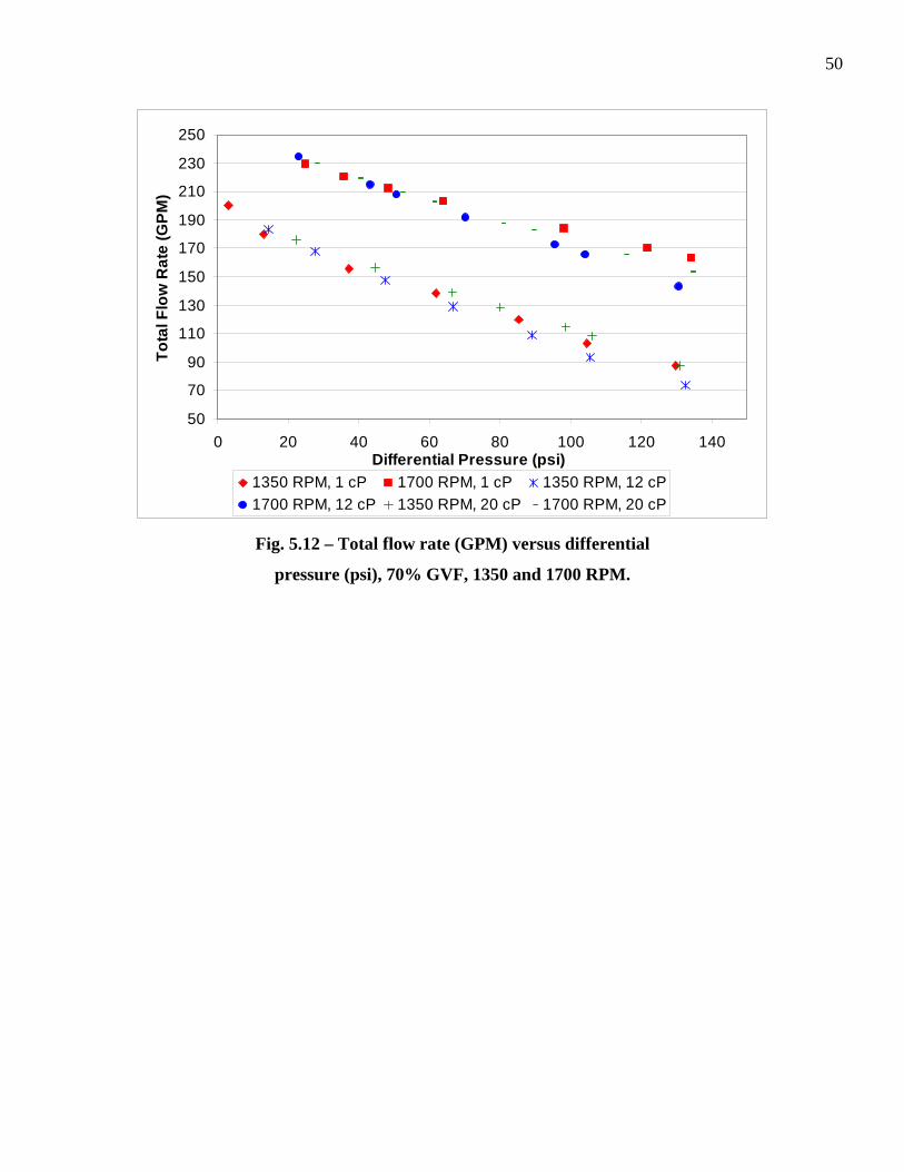
To determine whether more liquid in the pump would produce the expected
performance, further tests at 70% GVF were conducted. The results are shown in Fig.
5.12. Similar performance to the tests conducted under wet-gas conditions was observed.
50
50
70
90
110
130
150
170
190
210
230
250
0 20 40 60 80 100 120 140Differential Pressure (psi)
Tota
l Flo
w R
ate
(GPM
)
1350 RPM, 1 cP 1700 RPM, 1 cP 1350 RPM, 12 cP1700 RPM, 12 cP 1350 RPM, 20 cP 1700 RPM, 20 cP
Fig. 5.12 – Total flow rate (GPM) versus differential
pressure (psi), 70% GVF, 1350 and 1700 RPM.
51
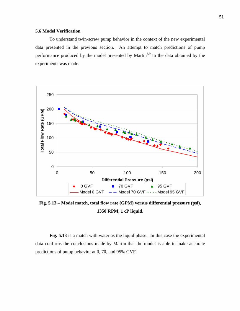
5.6 Model Verification
To understand twin-screw pump behavior in the context of the new experimental
data presented in the previous section. An attempt to match predictions of pump
performance produced by the model presented by Martin8,9 to the data obtained by the
experiments was made.
0
50
100
150
200
250
0 50 100 150 200
Differential Pressure (psi)
Tota
l Flo
w R
ate
(GPM
)
0 GVF 70 GVF 95 GVFModel 0 GVF Model 70 GVF Model 95 GVF
Fig. 5.13 – Model match, total flow rate (GPM) versus differential pressure (psi),
1350 RPM, 1 cP liquid.
Fig. 5.13 is a match with water as the liquid phase. In this case the experimental
data confirms the conclusions made by Martin that the model is able to make accurate
predictions of pump behavior at 0, 70, and 95% GVF.

52
Fig. 5.14 is the base case at 0% GVF and a 1 cP liquid. The model match is
excellent since the linear regression used to obtain the effect clearance size is based on
given data at this same condition. We are essentially giving the model this solution from
which other predictions at new operating situations are made.
0
50
100
150
200
250
0 50 100 150 200
Differential Pressure (psi)
Tota
l Flo
w R
ate
(GPM
)
0 GVF Model 0 GVF
Fig. 5.14 – Model match, total flow rate (GPM) versus differential pressure (psi),
0% GVF, 1350 RPM, 1 cP liquid.
53
0
50
100
150
200
250
0 50 100 150 200
Differential Pressure (psi
Tota
l Flo
w R
ate
(GPM
)
70 GVF Model 70 GVF
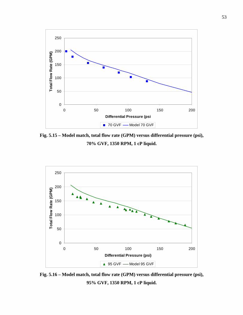
Fig. 5.15 – Model match, total flow rate (GPM) versus differential pressure (psi),
70% GVF, 1350 RPM, 1 cP liquid.
0
50
100
150
200
250
0 50 100 150 200
Differential Pressure (psi)
Tota
l Flo
w R
ate
(GPM
)
95 GVF Model 95 GVF
Fig. 5.16 – Model match, total flow rate (GPM) versus differential pressure (psi),
95% GVF, 1350 RPM, 1 cP liquid.

54
Fig. 5.15 and Fig. 5.16 are the model matches at 70 and 95% GVF. In both cases,
there is a slight amount of overestimation by the model. The overestimation is more
severe at lower differential pressures and for higher GVF.
When the liquid viscosity is increased to 9 cP, the model begins drastically
overestimating pump performance at all GVF, Fig. 5.17. An increasing trend in total
flow rate is predicted by the model with increasing GVF. This trend is opposite to what
was observed experimentally with a drop in performance with increasing starting at
higher differential pressures.
0
50
100
150
200
250
0 50 100 150 200Differential Pressure (psi)
Tota
l Flo
w R
ate
(GPM
)
0 GVF 70 GVF 95 GVFModel 0 GVF Model 70 GVF Model 95 GVF
Fig. 5.17 – Model match, total flow rate (GPM) versus differential pressure (psi),
1350 RPM, 9 cP liquid.

55
0
50
100
150
200
250
0 50 100 150 200Differential Pressure (psi)
Tota
l Flo
w R
ate
(GPM
)
0 GVF 70 GVF 95 GVFModel 0 GVF Model 70 GVF Model 95 GVF
Fig. 5.18 – Model match, total flow rate (GPM) versus differential pressure (psi),
1350 RPM, 24 cP liquid.
Fig. 5.18 is an attempt to match data at 24 cP. The model begins experiencing
severe difficulties, predicting a sharp discontinuity for the pump curve at each GVF.
These discontinuities are the result of a predicted transition between laminar and
turbulent flow.
Assuming that there is a problem with flow regime transitions, a match was
attempted using only the laminar or turbulent solution. The laminar solution produced an
unsatisfactory match. First overestimating and then underestimating pump performace,
Fig. 5.19.

56
0
50
100
150
200
250
0 20 40 60 80 100 120 140 160
Differential Pressure (psi)
Tota
l Flo
w R
ate
(GPM
)
0 GVF 70 GVF 95 GVF
0 GVF, Model 70 GVF, Model 95 GVF, Model
Fig. 5.19 – Model match, total flow rate (GPM) versus differential pressure (psi),
1350 RPM, 24 cP liquid, laminar flow only.
The turbulent solution was even more inaccurate. In all cases the predicted pump
curve was much higher than the experimental data, Fig. 5.20. Therefore, the conclusion
can be made that the poor matches at this viscosity are not caused purely by the flow
regime transition, though it is certainly one of the more glaring issues.

57
0
50
100
150
200
250
0 50 100 150 200
Differential Pressure (psi)
Tota
l Flo
w R
ate
(GPM
)
0 GVF 70 GVF 95 GVF
0 GVF, Model 70 GVF, Model 95 GVF, Model
Fig. 5.20 – Model match, total flow rate (GPM) versus differential pressure (psi),
1350 RPM, 24 cP liquid, turbulent flow only.

58
5.7 Viscosity Correction
Part of the reason that increased liquid viscosity is not having the expected effect
may be the non-Newtonian and temperature thinning properties of the gel used. The
shear imparted on a fluid within a twin-screw pump is thought to be small. Nevertheless,
some shear is being applied on the fluid as it moves through the narrow clearances.
Additionally, temperature increases due to viscous effects and gas compression further
reduce the effectiveness of the gel.
Since the Martin model does not have the ability to compensate for temperature
and shear effects using fluid rheology data. An attempt to determine the actual liquid
viscosity in the pump was made by matching pure liquid data with model prediction
made with lower viscosities. Fig. 5.21 shows that data of a 9 cP gel corresponds to
viscosity slightly under 2 cP in the model.
0
50
100
150
200
250
0 50 100 150 200
Differential Pressure (psi)
Tota
l Flo
w R
ate
(GPM
)
0 GVF, 9 cP Model 1 cP Model 2 cPModel 3 cP Model 4 cP Model 9 cP
Fig. 5.21 – Viscosity match, total flow rate (GPM) versus differential pressure (psi),
1350 RPM, 9 cP.
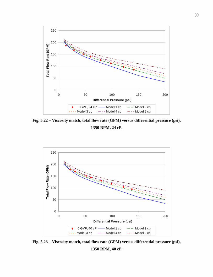
59
0
50
100
150
200
250
0 50 100 150 200
Differential Pressure (psi)
Tota
l Flo
w R
ate
(GPM
)
0 GVF, 24 cP Model 1 cp Model 2 cpModel 3 cp Model 4 cp Model 9 cp
Fig. 5.22 – Viscosity match, total flow rate (GPM) versus differential pressure (psi),
1350 RPM, 24 cP.
0
50
100
150
200
250
0 50 100 150 200
Differential Pressure (psi)
Tota
l Flo
w R
ate
(GPM
)
0 GVF, 40 cP Model 1 cp Model 2 cpModel 3 cp Model 4 cp Model 9 cp
Fig. 5.23 – Viscosity match, total flow rate (GPM) versus differential pressure (psi),
1350 RPM, 40 cP.
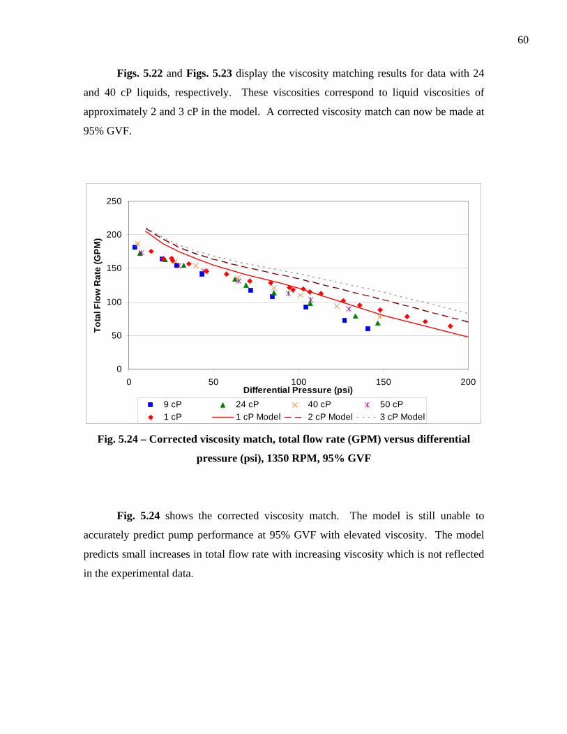
60
Figs. 5.22 and Figs. 5.23 display the viscosity matching results for data with 24
and 40 cP liquids, respectively. These viscosities correspond to liquid viscosities of
approximately 2 and 3 cP in the model. A corrected viscosity match can now be made at
95% GVF.
0
50
100
150
200
250
0 50 100 150 200Differential Pressure (psi)
Tota
l Flo
w R
ate
(GPM
)
9 cP 24 cP 40 cP 50 cP1 cP 1 cP Model 2 cP Model 3 cP Model
Fig. 5.24 – Corrected viscosity match, total flow rate (GPM) versus differential
pressure (psi), 1350 RPM, 95% GVF
Fig. 5.24 shows the corrected viscosity match. The model is still unable to
accurately predict pump performance at 95% GVF with elevated viscosity. The model
predicts small increases in total flow rate with increasing viscosity which is not reflected
in the experimental data.

61
5.8 Conclusions and Recommendations
New data obtained at high GVF does not confirm earlier findings. Instead of an
increase in pump flow rate with higher viscosity there is no change and even a drop in
total flow rate and volumetric efficiency. The new data suggest that at high GVF,
viscosity is not a dominant parameter. Though the thinning behavior of the gel reduces
the effect that it has on the pump system, it does not completely explain the trends
observed.
What is likely is that at high GVF, the liquid sealing around the chambers is being
lost, resulting in multiphase flow in the clearances. This would explain why the Martin
model which assumes pure liquid slip flow cannot provide adequate predictions. The
need for models to include multiphase flow effects in the clearances has been mentioned
before both by Prang & Cooper13 and Rausch14.
We can conclude that for the Martin model to work under wet-gas conditions it
must be modified to use real fluid property data to adjust the viscosity in each chamber.
The model must also be able to account for multiphase flow in the clearances. A partial
solution to this problem has been presented by Vetter et al.10 in the form of an effective
viscosity based on gas density and liquid viscosity.
Additionally, the recirculation chamber of the Bornemann pump must be taken
into account. Internal liquid recirculation would lower the actual GVF in the pump
which may reduce any performance differences resulting from high GVF. Rausch et al.14
were able to design this pump feature into their model.
More tests should be conducted at higher differential pressures. Since some
spreading of the data was observed at higher differential pressures, going to even higher
differential pressures may produce interesting results. Discharge pressure from the
Bornemann pump may be limited by the piping at the Riverside facility. Testing at
viscosities higher than 50 cP should be performed. Currently our ability to test higher
viscosities is limited by the capacity of the centrifugal charging pumps. Testing with a
non-Newtonian and temperature resistant fluid would minimize shear and temperature
effects on pump performance and allow for less convoluted data.

62
CHAPTER VI
THROUGH-CASING INJECTION
This chapter presents the results and discussion of all work done on determining
the feasibility of the through-casing injection concept. Since experimental testing of
through-casing injection would require significant modifications to an expensive piece of
machinery, this problem could only be approached theoretically.
6.1 Injection Theory
The method used to model gas compression in twin-screw pumps was presented
in Chapter II. Eq. 2.2 is the system of equations that is solved to determine the pump’s
internal pressure profile at a given set of conditions. To simulate injection, the simplest
approach would be to model the injection as an additional slip flow term. A portion of
the modified system of equations can then be rewritten as:
( )11 1
1
1 0i ii i i in
i i
p ZV q q qp Z
−− −
−
⎛ ⎞⋅⋅ − + − + ⋅Δ⎜ ⎟⋅⎝ ⎠
j t = (6.1)
Where the additional injection flow rate, qinj, would be inserted depends on into
which chamber or chambers injection is desired. Implementing this injection term would
require the computer program solving the Martin model to be reworked. However a good
approximation of pump behavior with injection can be obtained using a simpler method.
Data on pump pressure profiles and liquid volumes in each chamber can be adjusted to
simulate injection.

63
0
50
100
150
200
250
1 2 3 4Position
Pres
sure
(psi
g)
0 GVF 20 GVF 40 GVF 60 GVF 80 GVF 90 GVF
Fig. 6.1 – Pressure profiles (psig), differential pressure 200 psi, 1800 RPM (after
Martin8).
Fig. 6.1 presents pressure profile solutions given by the Martin model for the
Bornemann pump operating at a differential pressure of 200 psi and a pump speed of
1800 RPM for different GVF. As the GVF increases the pressure profile becomes
increasingly nonlinear. The Bornemann pump has four chambers on each half of the
each of the two screws. This corresponds to four identical sets of four chambers moving
from the suction to the discharge, Fig. 2.1. Each of the chambers is indexed 1 through 4
with position 1 being the suction and position 4 being the discharge.
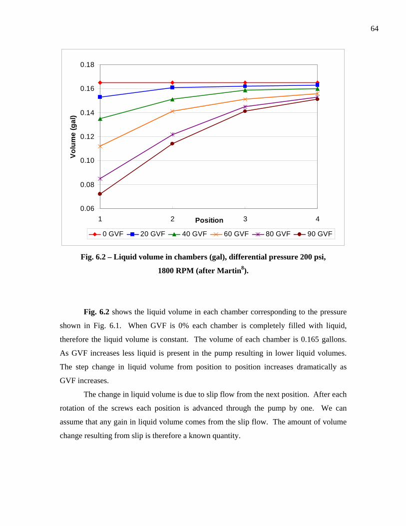
64
0.06
0.08
0.10
0.12
0.14
0.16
0.18
1 2 3 4Position
Volu
me
(gal
)
0 GVF 20 GVF 40 GVF 60 GVF 80 GVF 90 GVF
Fig. 6.2 – Liquid volume in chambers (gal), differential pressure 200 psi,
1800 RPM (after Martin8).
Fig. 6.2 shows the liquid volume in each chamber corresponding to the pressure
shown in Fig. 6.1. When GVF is 0% each chamber is completely filled with liquid,
therefore the liquid volume is constant. The volume of each chamber is 0.165 gallons.
As GVF increases less liquid is present in the pump resulting in lower liquid volumes.
The step change in liquid volume from position to position increases dramatically as
GVF increases.
The change in liquid volume is due to slip flow from the next position. After each
rotation of the screws each position is advanced through the pump by one. We can
assume that any gain in liquid volume comes from the slip flow. The amount of volume
change resulting from slip is therefore a known quantity.

65
Injection
Fig. 6.3 – Simplified injection model.
If each chamber in the pump is modeled as a piston with the liquid phase
compressing the gas phase, injection into this piston would increase the liquid volume
thereby increasing the overall pressure. Since the slip flow rates into and out of the
chamber are only functions of pressure, new slip flow rates can be calculated, Fig. 6.3.
For turbulent flow the slip flow can be calculated as: 0.57
slipq C p= ⋅Δ (6.2)
In the preceding equation, the characteristic clearance, C, can be assumed as
constant. Therefore, a proportional change in slip flow resulting from the injection can
be formulated as:
0.57
, 2 1
2 1
slip inj inj
slip
q p pq p p
+ −⎛ ⎞= ⎜ ⎟−⎝ ⎠
(6.3)

66
Using these two simple equations, the flow out of the chamber upstream and into
the downstream chamber from the chamber in which we are injecting can be adjusted for
a given increase in pressure in the injected chamber. The resulting changes in volume
will then allow a new pressure profiles to be calculated.
Given a specific pressure increase in the injected chamber, the volume and
therefore the flow rate necessary to cause the increase in pressure can be calculated. The
flow rate is calculated by simply multiplying the volume of injection needed by the pump
speed. The amount of power needed for injection can then be easily calculated:
1714Q Php Δ
= (6.4)
In this equation the flow rate, Q, is given in gallons per minute and the pressure
head, ΔP, in psi. The calculated power values are subject to injection pump efficiency.
Injection pressure needed is calculated assuming injection fluid initially at atmospheric
pressure to give a worse case scenario. Taking fluid pressurized liquid from the suction
or discharge side would dramatically decrease the amount of power needed. If liquid at
suction pressure were used, no additional boosting would be needed since the discharge
pressure is higher than the injection pressure. If liquid were taken from suction then a
minimal amount of power would be needed since the pressure difference between
positions 1 and 2 is small. In some cases using fluid from the suction would decrease the
power needed by half.

67
6.2 Feasibility Study
For this study injection will occur at position 2 only. Injection at this position
should create a more linear pressure profile by adding compression to chambers which
previously contributed little at high GVF. Fig. 6.4 shows the calculated pressure profiles
starting from the base case of 90% GVF with no injection and adding various pressure
increases in position 2 resulting from injection.
0
50
100
150
200
250
300
1 2 3Position
Pres
sure
(psi
g)
4
No Injection 10 psi 20 psi 30 psi 40 psi 50 psi
Fig. 6.4 – Pressure profiles (psig) with injection, 90% GVF,
differential pressure 200 psi, 1800 RPM.
As the pressure in position 2 is increased, a corresponding increase in discharge
pressure at position 4 is observed. The pressure profile also becomes slightly more linear
with increasing injection. The suction pressure is also affected in this model since it is
considered a closed chamber. In actuality, the suction pressure may not change.

68
0.06
0.07
0.08
0.09
0.10
0.11
0.12
0.13
0.14
0.15
0.16
1 2 3Position
Volu
me
(gal
)
4
No Injection 10 psi 20 psi 30 psi 40 psi 50 psi
Fig. 6.5 – Liquid volume in chambers (gal) with injection, 90% GVF,
differential pressure 200 psi, 1800 RPM.
Corresponding liquid volumes in the chambers increase as expected as we
introduce more liquid into the pump, Fig. 6.5. As more liquid is injected the liquid
volumes begin to approach a more even profile. The liquid volume at position 4 provides
a limiting parameter to injection. Eventually, no more liquid and subsequently no more
pressure can be introduced at the discharge.

69
0
5
10
15
20
25
30
35
0 10 20 30 40 50 6
Pressure Increase at Position 2 (psi)
Pres
sure
Boo
st a
t Dis
char
ge (p
si)
0
Fig. 6.6 – Pressure boost at position 2 (psi) versus pressure boost at discharge (psi),
90% GVF, differential pressure 200 psi, 1800 RPM.
As pressure is introduced into position 2 the total pressure boost at the discharge
increases at a declining rate, Fig. 6.6. An injection pressure increase of 50 psi will result
in a total pressure boost of only 31 psi.
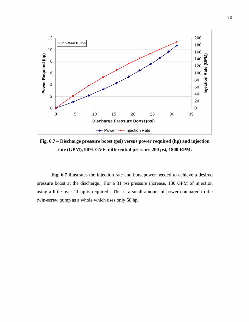
70
50 hp Main Pump
0
2
4
6
8
10
12
0 5 10 15 20 25 30 35
Discharge Pressure Boost (psi)
Pow
er R
equi
red
(hp)
0
20
40
60
80
100
120
140
160
180
200
Inje
ctio
n R
ate
(GPM
)
Power Injection Rate
Fig. 6.7 – Discharge pressure boost (psi) versus power required (hp) and injection
rate (GPM), 90% GVF, differential pressure 200 psi, 1800 RPM.
Fig. 6.7 illustrates the injection rate and horsepower needed to achieve a desired
pressure boost at the discharge. For a 31 psi pressure increase, 180 GPM of injection
using a little over 11 hp is required. This is a small amount of power compared to the
twin-screw pump as a whole which uses only 50 hp.

71
50 hp Main Pump0%
2%
4%
6%
8%
10%
12%
14%
16%
0 2 4 6 8 10 12
Power (hp)
Pres
sure
Incr
ease
(%)
Fig. 6.8 – Power required (hp) versus pressure increase (%), 90% GVF, differential
pressure 200 psi, 1800 RPM.
As more power is expended, a declining amount of pressure boost above 200 psi
is observed. 11 hp is needed to increase the differential pressure provided by the twin-
screw pump by about 14%, Fig. 6.8.
Similar results can be seen for 80% GVF, Fig. 6.9 and Fig. 6.10, and 60% GVF,
Fig. 6.11 and Fig. 6.12. For injection at 80% GVF the results are almost identical to
injection at 90%. The same basic trends are observed. Injection at 60% GVF begins to
cause problems. At 60% GVF, the amount of the liquid already present in the pump is
such that a given amount of injection has little effect on the chambers closer to the
discharge. With a large amount of injection, the pressure profiles start to become more
discontinuous and total pressure boost is reaches its limit.
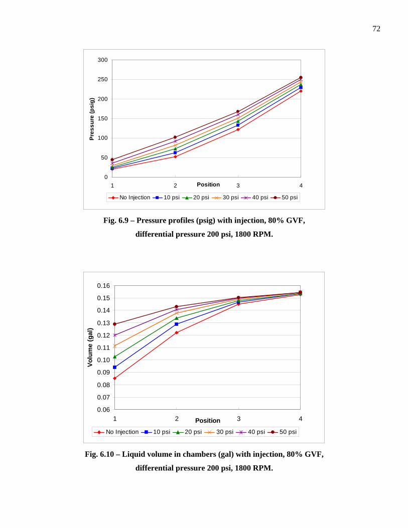
72
0
50
100
150
200
250
300
1 2 3 4Position
Pres
sure
(psi
g)
No Injection 10 psi 20 psi 30 psi 40 psi 50 psi
Fig. 6.9 – Pressure profiles (psig) with injection, 80% GVF,
differential pressure 200 psi, 1800 RPM.
0.06
0.07
0.08
0.09
0.10
0.11
0.12
0.13
0.14
0.15
0.16
1 2 3Position
Volu
me
(gal
)
4
No Injection 10 psi 20 psi 30 psi 40 psi 50 psi
Fig. 6.10 – Liquid volume in chambers (gal) with injection, 80% GVF,
differential pressure 200 psi, 1800 RPM.
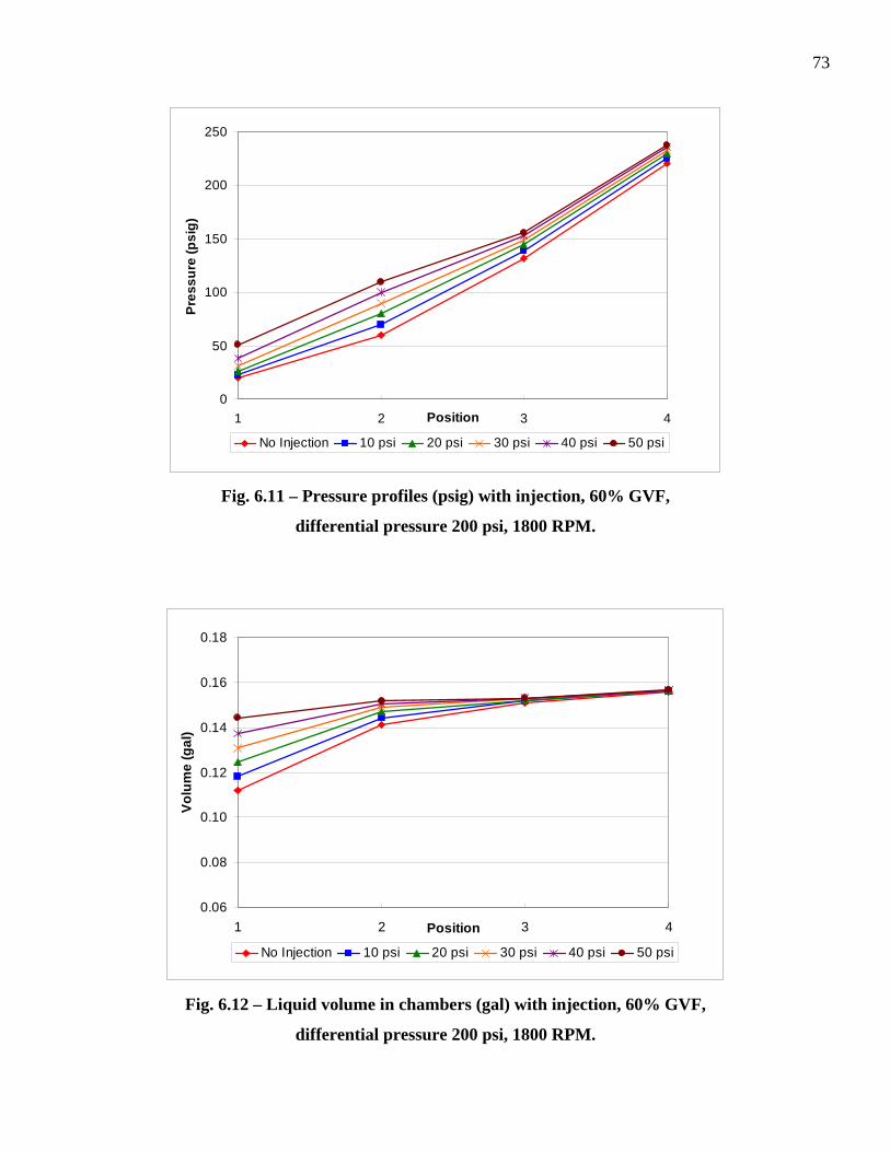
73
0
50
100
150
200
250
1 2 3Position
Pres
sure
(psi
g)
4
No Injection 10 psi 20 psi 30 psi 40 psi 50 psi
Fig. 6.11 – Pressure profiles (psig) with injection, 60% GVF,
differential pressure 200 psi, 1800 RPM.
0.06
0.08
0.10
0.12
0.14
0.16
0.18
1 2 3 4Position
Volu
me
(gal
)
No Injection 10 psi 20 psi 30 psi 40 psi 50 psi
Fig. 6.12 – Liquid volume in chambers (gal) with injection, 60% GVF,
differential pressure 200 psi, 1800 RPM.

74
020406080
100120140160180200
0 10 20 30 40 50 6
Pressure Increase at Position 2 (psi)
Inje
ctio
n R
ate
(GPM
)
0
90 GVF 80 GVF 60 GVF
Fig. 6.13 – Pressure increase at position 2 (psi) versus injection rate (GPM),
differential pressure 200 psi, 1800 RPM.
Fig. 6.13 displays the injection rate needed to produce the desired pressure
increase at position 2. As GVF decreases less injection is required. This is due to the
fact that there is more liquid present in each chamber at lower GVF.
To give a perspective of the amount of liquid needed. The total flow rate of the
pump operating under the given conditions and at 90% GVF is 181.5 GPM. The total
liquid flow rate is therefore only 18.15 GPM. The liquid injection needed can therefore
be far larger than the liquid flow rate of the twin-screw pump.
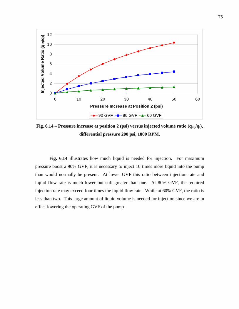
75
0
2
4
6
8
10
12
0 10 20 30 40 50 6
Pressure Increase at Position 2 (psi)
Inje
cted
Vol
ume
Rat
io (q
inj/q
l)
0
90 GVF 80 GVF 60 GVF
Fig. 6.14 – Pressure increase at position 2 (psi) versus injected volume ratio (qinj/ql),
differential pressure 200 psi, 1800 RPM.
Fig. 6.14 illustrates how much liquid is needed for injection. For maximum
pressure boost a 90% GVF, it is necessary to inject 10 times more liquid into the pump
than would normally be present. At lower GVF this ratio between injection rate and
liquid flow rate is much lower but still greater than one. At 80% GVF, the required
injection rate may exceed four times the liquid flow rate. While at 60% GVF, the ratio is
less than two. This large amount of liquid volume is needed for injection since we are in
effect lowering the operating GVF of the pump.
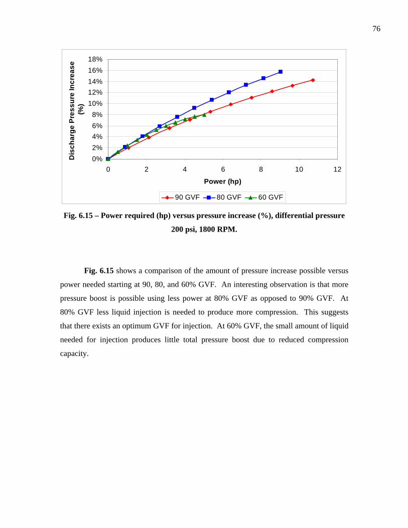
76
0%2%4%6%8%
10%12%14%16%18%
0 2 4 6 8 10
Power (hp)
Dis
char
ge P
ress
ure
Incr
ease
(%
)
12
90 GVF 80 GVF 60 GVF
Fig. 6.15 – Power required (hp) versus pressure increase (%), differential pressure
200 psi, 1800 RPM.
Fig. 6.15 shows a comparison of the amount of pressure increase possible versus
power needed starting at 90, 80, and 60% GVF. An interesting observation is that more
pressure boost is possible using less power at 80% GVF as opposed to 90% GVF. At
80% GVF less liquid injection is needed to produce more compression. This suggests
that there exists an optimum GVF for injection. At 60% GVF, the small amount of liquid
needed for injection produces little total pressure boost due to reduced compression
capacity.

77
6.3 Conclusions
The feasibility of through-casing injection has been demonstrated. This method
has been shown capable of producing an increase in differential pressure of up to 16%.
At high initial GVF, pressure profiles can become more linear with injection. The
injection rate required to produce the pressure increases needed decreases as GVF
decreases. The amount of liquid at the discharge is the limiting factor for the maximum
injection rate possible.
The potential of this method has been shown. Further modeling studies and
experimental tests should be conducted. The ability of this method to produce more
linear pressure profiles may solve some of the vibration problems observed in the field at
high GVF. This method also provides a means of producing more pressure boost from an
existing pump. The use of injection of a cooler liquid to reduce internal temperature
increases at high GVF is another possible application of this method that should be
investigated.
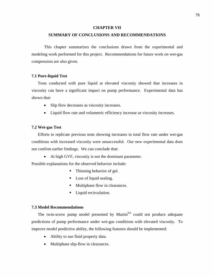
78
CHAPTER VII
SUMMARY OF CONCLUSIONS AND RECOMMENDATIONS
This chapter summarizes the conclusions drawn from the experimental and
modeling work performed for this project. Recommendations for future work on wet-gas
compression are also given.
7.1 Pure-liquid Test
Tests conducted with pure liquid at elevated viscosity showed that increases in
viscosity can have a significant impact on pump performance. Experimental data has
shown that:
• Slip flow decreases as viscosity increases.
• Liquid flow rate and volumetric efficiency increase as viscosity increases.
7.2 Wet-gas Test
Efforts to replicate previous tests showing increases in total flow rate under wet-gas
conditions with increased viscosity were unsuccessful. Our new experimental data does
not confirm earlier findings. We can conclude that:
• At high GVF, viscosity is not the dominant parameter.
Possible explanations for the observed behavior include:
Thinning behavior of gel.
Loss of liquid sealing.
Multiphase flow in clearances.
Liquid recirculation.
7.3 Model Recommendations
The twin-screw pump model presented by Martin8,9 could not produce adequate
predictions of pump performance under wet-gas conditions with elevated viscosity. To
improve model predictive ability, the following features should be implemented:
• Ability to use fluid property data.
• Multiphase slip-flow in clearances.

79
• Effective mixture viscosity of slip fluid.
Discussed by Cooper & Prang13 and Vetter et al.10,11
• Bornemann pump liquid recirculation.
Discussed by Rausch et. al14
7.4 Experiment Recommendations
In order to fully explore wet-gas compression with twin-screw pumps and twin-screw
pump behavior with high viscosity liquids further tests should be conducted with
modifications to the experimental facility to accommodate:
• Higher boost pressures, > 150 psi.
• Higher viscosities, > 50 cp.
Additionally, the use of a non-temperature thinning, Newtonian liquid would
eliminate the complications created by using guar gel.
7.5 Through-Casing Injection Feasibility
The modeling study of through casing injection has shown that:
• The feasibility of through-casing injection has been demonstrated.
• Discharge pressure can be boosted by a maximum of 16%.
• Pressure profiles can become more linear with injection.
• The required injection rate decreases with lower GVF.
• Amount of injection is limited by the volume of liquid in the final chamber.

80
NOMENCLATURE
Ac circumferential area (ft2) c radial clearance (in.)
cc circumferential clearance (in.)
C effective clearance (dimensionless)
D displacement per revolution (gal/rev)
Dc screw external diameter (in.)
K flow consistency index (cPn)
lh circumferential gap (in.)
M molecular weight (lb/lbmole) .
m mass flow rate (lb/min)
N pump speed (RPM)
n flow behavior index (dimensionless)
nt number of threads (dimensionless)
nu number of chambers (dimensionless) p pressure (psi) q actual pump flow rate (GPM)
qg gas flow rate (GPM)
qinj injection flow rate (GPM)
ql liquid flow rate (GPM)
qslip slip flow rate (GPM)
qTH theoretical pump flow rate (GPM)
R gas constant

81
s pitch (in./rev)
T temperature (°F)
V volume (gallons) v velocity (ft/sec) z compressibility factor (dimensionless) γ shear rate (sec-1) vη volumetric efficiency (dimensionless) ρg gas density (lb/gal) ρl liquid density (lb/gal) μ apparent viscosity (cP)

82
REFERENCES
1. Scott, S.L.: “Utilization of Multiphase Pumping in the Oil and Gas Industry,”
paper presented at the 2004 Advances in Multiphase Separation and Multiphase
Pumping Technologies Seminar, Aberdeen (June 30, 2004).
2. Scharf, A., Raush, T., Vauth, Th., and Mewes, D.: “Investigation on Conveying
Characteristics of Multiphase Twin Screw Pumps,” presentation given at the 2005
Multiphase Pumping & Metering Technologies Conference, Manama, Bahrain
(November 2005).
3. Martin, A.M. and Scott, S.L.: “Modeling Reservoir/Tubing/Pump Interaction
Identifies Best Candidates for Multiphase Pumping,” paper SPE 77500 presented
at the 2002 Annual Technical Conference and Exhibition, San Antonio, Texas, 29
September – 2 October.
4. Wilkinson, D.: “CNRL’s Twin Screw Multiphase Pump Experience 2002-2006,”
presentation given at the 2006 Texas A&M Multiphase Pump User Roundtable-
Canada, Calgary (June 12, 2006).
5. Dick, C. and Speirs, B.: “Imperial Oil Operating Experience with Multiphase and
Mass Transfer Pumps in Wet Gas Compression at Cold Lake,” presentation given
at the 2006 Texas A&M Multiphase Pump User Roundtable- Canada, Calgary
(June 12, 2006).
6. Singh, A.: “Modeling Twin-Screw Multiphase Pump Performance during Periods
of High Gas Volume Fraction,” MS thesis, Texas A&M U., College Station,
Texas (2003).

83
7. Singh, A.: “Operability and Performance of Twin-Screw Multiphase Pumps
During Wet-Gas Conditions,” presentation given at the 2005 National
Engineering Laboratories, United Kingdom and Texas A&M Multiphase Pump
User Roundtable- Europe, Aberdeen (August 31, 2005).
8. Martin, A.M.: “Multiphase Twin-Screw Pump Modeling for the Oil and Gas
Industry,” PhD dissertation, Texas A&M U., College Station, Texas (2003).
9. Martin, A.M.: “Multiphase Twin-Screw Pump Modeling for the Oil and Gas
Industry,” presentation given at the 2005 National Engineering Laboratories,
United Kingdom and Texas A&M Multiphase Pump User Roundtable- Europe,
Aberdeen (August 31, 2005).
10. Vetter, G. and Wincek, M.: “Performance Prediction of Twin-Screw Pumps for
Two-Phase Gas/Liquid Flow,” Pumping Machinery, ASME (1993) FED 154,
331-340.
11. Vetter, G., Wirth, W., Korner, H., and Pregler, S.: “Multiphase Pumping with
Twin-Screw Pumps- Understand and Model Hydrodynamics and Hydroabrasive
Wear,” Proc., 17th International Pump Users Symposium, Houston (1999) 153-
169.
12. Egashira, K., Shoda, S., Tochikawa, T., and Furukawa, A.: “Backflow in Twin-
Screw-Type Multiphase Pump,” SPEPF (February 1998) 64.
13. Prang, A.J. and Cooper, P.: “Enhanced Multiphase Predictions in Twin-Screw
Pumps,” Proc., 21st International Pump Users Symposium, Houston (2004) 69-76.

84
14. Rausch, T., Vauth, Th., Brandt, J-U., and Mewes, D.: “A Model for the
Delivering Characteristic of Multiphase Pumps,” paper presented at the 4th
Annual North American Conference on Multiphase Technology, Banff, Canada
(June 3-4, 2004).
15. Toma, P.: “Analysis of Multiphase Pumping Instabilities Observed in Steam-
Assisted Oil Recovery Fields,” Proc., International Mechanical Engineers
Congress and Exhibition, Orlando, Florida (2005) 1-14.
16. Rohlfing, G. and Muller-Link, D.: “Twin-Screw Rotors - 2nd Generation for
Increased Efficiency,” presentation given at the 2006 Texas A&M Multiphase
Pump User Roundtable-Canada, Calgary (June 12, 2006).
17. “NPV Subsea Test Results,” Nuovo Pignone SpA, Florence, Italy (June 2001).
18. Fraino and Santibanez: “Effect of Speed Increase and Clearance Reduction in the
Performance of Multiphase Twin Screw Pumps,” presentation given at the 2006
Texas A&M Multiphase Pump User Roundtable-Canada, Calgary (June 12,
2006).

85
APPENDIX A
STUDY OF TWIN-SCREW PUMP CLEARANCES
This section features a short study of pump clearance sizes using the model
presented by Martin8,9. The Martin model uses linear regression on pure water
performance data to determine a value for the effective clearance size, C, within a pump.
The linear regression gives a value of C that is consistent with the equation for pump
flow rate with turbulent slip flow in the clearances
(A.1) 0.57
THq q C p= − ⋅Δ For laminar flow C can also be calculated by:
1.25
0.75 0.25
240.066
th t
ch
ncC l c ns nρ μ
⎛ ⎞⋅= ⋅ ⋅ ⋅ ⋅⎜ ⎟⋅ ⋅⎝ ⎠
(A.2)
In Eq, A.2, lh, c, and s are all measurements of screw geometry. C is therefore a lumped
parameter with no meaningful units. Nominally, the Bornemann pump examined has a C
value of around 9.5. Unfortunately, reducing this C value to specific measurements of
pump clearances cannot be easily done. So the effect of reducing the C value itself will
be examined to give the effect of proportional changes in the clearance sizes.
As shown in Fig. A.1 and Fig. A.2, reducing the C value produces increases in
flow rate and decreases in slip flow rate at 0% GVF. Therefore volumetric efficiency
increases as clearance are narrowed. Fig. A.3 and Fig. A.4 show similar results for 95%
GVF. The effect of reducing clearances is even more pronounced at this higher GVF.
Fig. A.5 shows a comparison of the reduction of clearance sizes. Reducing the
clearances by a third can more than double the flow rate possible.
Although narrower clearances produce more efficient pump performance, they are
not necessary desirable. Pump clearances are a tradeoff between efficiency and
reliability. A pump’s ability to tolerate entrained solids such as sand is due in large part
to the clearance sizes. Additionally, metal on metal contact due to shaft deflection is far
more likely with narrower clearances. The results of this study are consistent with field
data presented by Fraino & Santibanez18.
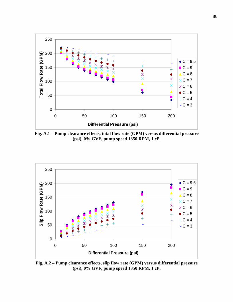
86
0
50
100
150
200
250
0 50 100 150 200
Differential Pressure (psi)
Tota
l Flo
w R
ate
(GPM
)
C = 9.5C = 9C = 8C = 7C = 6C = 5C = 4C = 3
Fig. A.1 – Pump clearance effects, total flow rate (GPM) versus differential pressure
(psi), 0% GVF, pump speed 1350 RPM, 1 cP.
0
50
100
150
200
250
0 50 100 150 200
Differential Pressure (psi)
Slip
Flo
w R
ate
(GPM
) C = 9.5C = 9C = 8C = 7C = 6C = 5C = 4C = 3
Fig. A.2 – Pump clearance effects, slip flow rate (GPM) versus differential pressure
(psi), 0% GVF, pump speed 1350 RPM, 1 cP.

87
0
50
100
150
200
250
0 50 100 150 200Differential Pressure (psi)
Tota
l Flo
w R
ate
(GPM
)
C = 9.5C = 9C = 8C = 7C = 6C = 5C = 4C = 3
Fig. A.3 – Pump clearance effects, total flow rate (GPM) versus differential pressure
(psi), 95% GVF, pump speed 1350 RPM, 1 cP.
020406080
100120140160180200
0 50 100 150 200
Differential Pressure (psi)
Slip
Flo
w R
ate
(GPM
) C = 9.5C = 9C = 8C = 7C = 6C = 5C = 4C = 3
Fig. A.4 – Pump clearance effects, slip flow rate (GPM) versus differential pressure
(psi), 95% GVF, pump speed 1350 RPM, 1 cP.
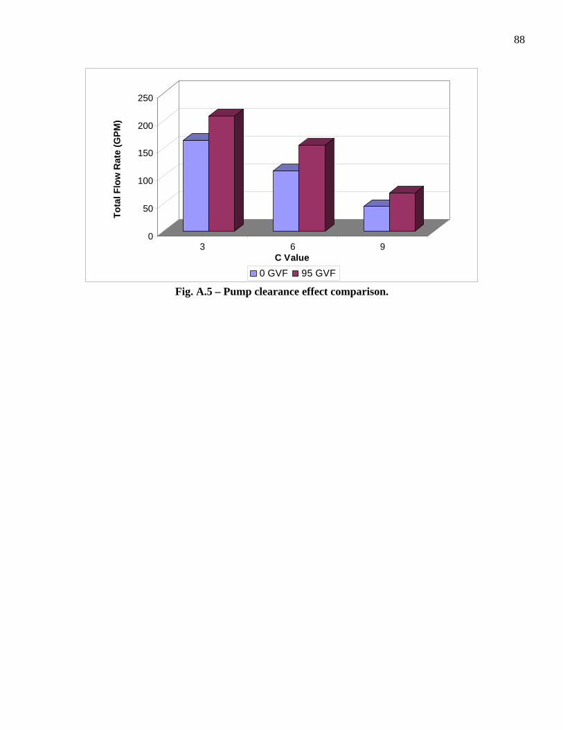
88
0
50
100
150
200
250
Tota
l Flo
w R
ate
(GPM
)
3 6 9C Value
0 GVF 95 GVF
Fig. A.5 – Pump clearance effect comparison.

89
APPENDIX B
0% GVF DATA
Table B.1 – 1 cP, 0% GVF, 1350 RPM. mg
(lbpm) T (F) ml
(lbpm) ρl
(ppg) PD
(psi) PS
(psi) TS (F)
TD (F)
ql (bbl/d)
qg (bbl/d) GVF
ql (GPM)
qg (GPM)
ΔP (psi)
0.027 88.24 1527.03 8.260 83.62 73.12 90.00 89.99 6339.58 19.41 0.003 185.12 0.57 10.50
0.023 88.71 1368.26 8.260 105.46 82.76 91.19 91.29 5680.04 14.85 0.003 165.86 0.43 22.70
0.026 88.77 1263.83 8.258 121.63 88.17 91.39 91.64 5247.81 15.27 0.003 153.24 0.45 33.47
0.020 89.33 1136.07 8.255 142.78 94.57 94.24 94.47 4718.98 11.22 0.002 137.79 0.33 48.22
0.022 88.82 1092.94 8.258 151.67 96.65 91.81 92.05 4538.16 12.04 0.003 132.51 0.35 55.01
0.019 88.94 961.55 8.259 177.31 102.17 92.38 92.52 3992.45 10.02 0.003 116.58 0.29 75.14
0.020 89.44 933.42 8.253 181.10 103.23 95.27 95.35 3878.25 10.23 0.003 113.24 0.30 77.88
0.019 89.05 856.82 8.257 199.27 106.03 92.93 93.26 3558.09 9.43 0.003 103.90 0.28 93.24
0.020 89.14 789.14 8.258 213.38 108.35 93.19 93.81 3276.94 9.89 0.003 95.69 0.29 105.03
0.021 89.23 671.41 8.255 239.90 111.74 93.72 94.56 2788.91 10.07 0.004 81.44 0.29 128.16
0.020 89.74 1370.38 8.252 70.34 47.72 95.67 95.70 5694.40 21.69 0.004 166.28 0.63 22.62
0.023 89.94 1246.87 8.251 86.93 52.33 96.01 96.13 5181.82 22.74 0.004 151.31 0.66 34.60
0.016 90.14 1096.63 8.251 110.42 57.24 96.30 96.31 4557.68 15.11 0.003 133.08 0.44 53.18
0.019 90.19 989.99 8.250 128.77 60.17 96.15 96.47 4114.83 16.83 0.004 120.15 0.49 68.61
0.017 90.22 793.62 8.249 166.80 64.82 96.20 96.88 3298.99 13.69 0.004 96.33 0.40 101.98
0.021 90.30 595.50 8.251 211.59 68.47 96.46 97.51 2474.93 16.55 0.007 72.27 0.48 143.13
0.007 93.71 1320.15 8.267 66.35 36.23 82.68 82.57 5476.02 9.99 0.002 159.90 0.29 30.12
0.008 93.81 1235.90 8.268 78.60 39.11 82.97 82.93 5125.64 9.94 0.002 149.67 0.29 39.50
0.006 93.75 1078.15 8.269 105.97 44.41 83.00 83.22 4470.66 6.67 0.001 130.54 0.19 61.55
0.007 93.55 946.43 8.269 132.83 48.26 83.60 83.73 3924.79 7.42 0.002 114.60 0.22 84.57
0.007 93.56 824.23 8.267 157.62 51.45 83.47 84.20 3418.72 6.75 0.002 99.83 0.20 106.17
0.009 93.63 740.89 8.268 177.57 53.45 83.97 84.57 3072.71 8.63 0.003 89.72 0.25 124.12
0.008 93.69 641.17 8.269 203.03 55.57 84.47 85.21 2658.87 7.91 0.003 77.64 0.23 147.45
0.013 95.61 1333.06 8.263 62.27 35.43 88.30 88.50 5531.92 19.05 0.003 161.53 0.56 26.83
0.014 95.82 1237.63 8.262 76.30 39.84 88.59 88.75 5136.27 18.21 0.004 149.98 0.53 36.46
0.016 95.94 1093.34 8.262 99.94 46.11 88.80 89.04 4537.77 17.84 0.004 132.50 0.52 53.83
0.016 95.99 965.41 8.263 124.65 51.64 88.86 89.27 4006.52 16.44 0.004 116.99 0.48 73.01
0.012 95.98 813.60 8.263 156.37 57.48 89.22 89.64 3376.23 10.50 0.003 98.59 0.31 98.89
0.013 95.99 719.09 8.262 177.70 60.57 89.13 90.03 2984.60 10.85 0.004 87.15 0.32 117.14
0.014 96.00 614.83 8.262 202.55 63.85 89.62 90.44 2551.75 11.68 0.005 74.51 0.34 138.69
0.011 95.94 529.46 8.261 224.18 66.07 89.66 90.94 2197.63 8.77 0.004 64.17 0.26 158.10

90
Table B.2 – 9 cP, 0% GVF, 1350 RPM. mg
(lbpm) T (F) ml
(lbpm) ρl
(ppg) PD
(psi) PS
(psi) TS (F)
TD (F)
ql (bbl/d)
qg (bbl/d) GVF
ql (GPM)
qg (GPM)
ΔP (psi)
0.008 85.08 1403.35 8.271 63.82 37.53 87.09 87.00 5818.24 10.93 0.002 169.89 0.32 26.29
0.009 85.36 1275.57 8.269 83.23 42.21 87.16 87.14 5289.42 11.24 0.002 154.45 0.33 41.02
0.009 85.67 1214.19 8.271 94.85 45.40 87.03 87.27 5033.71 10.26 0.002 146.98 0.30 49.46
0.010 86.03 1113.04 8.271 113.80 49.42 87.40 87.46 4614.42 10.30 0.002 134.74 0.30 64.38
0.010 86.17 1009.84 8.270 134.04 53.39 87.34 87.60 4186.98 9.62 0.002 122.26 0.28 80.65
0.009 86.16 937.76 8.270 149.50 56.19 87.48 87.78 3888.13 7.91 0.002 113.53 0.23 93.31
0.009 85.94 839.55 8.270 170.99 59.30 87.56 88.08 3481.09 8.15 0.002 101.65 0.24 111.69
0.008 85.62 782.97 8.270 184.07 60.90 87.51 88.31 3246.44 7.09 0.002 94.80 0.21 123.17
0.008 85.26 721.95 8.269 197.63 62.34 87.85 88.67 2993.68 6.49 0.002 87.42 0.19 135.30
0.007 84.89 627.93 8.270 218.46 64.08 88.11 89.19 2603.54 6.05 0.002 76.02 0.18 154.37
0.007 84.62 548.47 8.271 234.75 64.89 88.47 89.69 2273.96 5.67 0.002 66.40 0.17 169.86
Table B.3 – 26 cP, 0% GVF, 1350 RPM. mg
(lbpm) T (F) ml
(lbpm) ρl
(ppg) PD
(psi) PS
(psi) TS (F) TD (F) ql
(bbl/d) qg
(bbl/d) GVF ql
(GPM) qg
(GPM) ΔP
(psi)
0.012 115.69 1550.63 8.244 104.69 91.32 104.97 104.89 6449.29 7.17 0.001 188.32 0.21 13.36
0.012 115.76 1402.92 8.245 126.19 97.61 104.97 105.02 5834.27 6.72 0.001 170.36 0.20 28.58
0.012 115.79 1266.16 8.245 148.88 102.99 105.34 105.46 5265.59 6.15 0.001 153.76 0.18 45.89
0.012 115.86 1168.76 8.245 166.23 106.42 105.43 105.66 4860.81 6.30 0.001 141.94 0.18 59.80
0.011 115.95 1049.02 8.244 188.40 110.15 105.93 106.22 4363.29 5.25 0.001 127.41 0.15 78.25
0.012 116.16 938.21 8.244 211.12 113.23 106.19 106.67 3902.33 5.64 0.001 113.95 0.16 97.89
0.011 116.35 811.96 8.245 238.19 116.42 106.70 107.30 3376.83 5.04 0.001 98.60 0.15 121.77
0.013 116.49 714.08 8.243 259.51 118.48 107.12 107.87 2970.49 5.92 0.002 86.74 0.17 141.04
Table B.4 – 40 cP, 0% GVF, 1350 RPM. mg
(lbpm) T (F) ml
(lbpm) ρl
(ppg) PD
(psi) PS
(psi) TS (F) TD (F) ql
(bbl/d) qg
(bbl/d) GVF ql
(GPM) qg
(GPM) ΔP
(psi)
0.006 102.15 1489.44 8.244 91.82 70.15 102.75 102.81 6195.09 4.38 0.001 180.90 0.13 21.67
0.008 102.05 1412.04 8.245 106.24 75.71 103.14 103.16 5872.30 5.93 0.001 171.47 0.17 30.53
0.016 102.08 1260.54 8.246 136.17 84.60 103.45 103.48 5241.52 10.08 0.002 153.05 0.29 51.57
0.013 102.11 1198.78 8.247 149.73 89.21 103.81 104.04 4984.25 7.65 0.002 145.54 0.22 60.52
0.019 102.07 1085.07 8.247 173.52 93.84 104.31 104.48 4511.73 10.98 0.002 131.74 0.32 79.67
0.019 102.08 976.20 8.247 197.77 98.50 104.60 104.90 4058.89 10.34 0.003 118.52 0.30 99.26
0.015 102.10 863.22 8.245 227.77 106.36 104.98 105.49 3589.88 7.65 0.002 104.82 0.22 121.41
0.017 102.07 785.78 8.245 246.28 109.18 105.35 106.03 3267.81 8.24 0.003 95.42 0.24 137.10

91
Table B.5 – 1 cP, 0% GVF, 1700 RPM. mg
(lbpm) T (F) ml
(lbpm) ρl
(ppg) PD
(psi) PS
(psi) TS (F)
TD (F)
ql (bbl/d)
qg (bbl/d) GVF
ql (GPM)
qg (GPM)
ΔP (psi)
0.010 95.80 1681.97 8.265 89.16 46.96 85.04 85.10 6978.40 11.22 0.002 203.77 0.33 42.21
0.008 95.40 1623.42 8.266 100.10 50.37 85.45 85.54 6734.85 8.57 0.001 196.66 0.25 49.73
0.010 95.24 1500.43 8.265 126.32 59.97 86.03 86.12 6224.72 8.70 0.001 181.76 0.25 66.35
0.009 95.24 1387.65 8.264 151.55 67.76 86.24 86.56 5757.59 7.07 0.001 168.12 0.21 83.79
0.011 95.21 1314.06 8.264 169.51 73.38 86.52 86.88 5452.21 7.74 0.001 159.20 0.23 96.13
0.012 95.18 1242.58 8.264 188.27 78.50 86.77 87.33 5156.03 8.18 0.002 150.56 0.24 109.77
0.014 95.25 1159.77 8.264 208.65 83.50 87.44 87.77 4812.57 8.87 0.002 140.53 0.26 125.15
0.017 95.38 1087.62 8.263 227.23 87.64 87.43 88.20 4513.40 9.99 0.002 131.79 0.29 139.60
0.018 95.51 969.08 8.262 256.59 93.80 88.06 88.75 4021.83 9.91 0.002 117.44 0.29 162.79
0.031 95.65 902.32 8.262 272.30 97.25 88.33 89.29 3745.07 16.47 0.004 109.36 0.48 175.05
Table B.6 – 9 cP, 0% GVF, 1700 RPM. mg
(lbpm) T (F) ml
(lbpm) ρl
(ppg) PD
(psi) PS
(psi) TS (F)
TD (F)
ql (bbl/d)
qg (bbl/d) GVF
ql (GPM)
qg (GPM)
ΔP (psi)
0.018 79.89 1729.51 8.268 89.29 45.77 88.93 89.05 7173.04 20.42 0.003 209.45 0.60 43.52
0.014 79.44 1649.39 8.268 105.13 51.06 88.97 89.19 6840.29 13.95 0.002 199.74 0.41 54.07
0.012 78.93 1546.64 8.269 128.29 59.18 89.20 89.33 6413.60 10.46 0.002 187.28 0.31 69.11
0.012 78.48 1458.56 8.268 149.92 66.08 89.33 89.58 6048.88 9.19 0.002 176.63 0.27 83.84
0.010 77.46 1365.96 8.268 172.33 71.46 89.72 90.07 5664.91 7.41 0.001 165.42 0.22 100.87
0.010 77.05 1267.60 8.268 198.44 78.87 90.03 90.32 5256.88 6.60 0.001 153.50 0.19 119.57
0.011 76.69 1203.46 8.267 215.67 83.23 90.08 90.60 4992.04 7.02 0.001 145.77 0.20 132.45
0.010 76.40 1122.04 8.268 238.00 88.41 90.35 90.91 4653.64 5.66 0.001 135.89 0.17 149.59
0.009 76.03 1022.63 8.267 267.34 94.90 90.65 91.39 4241.83 5.15 0.001 123.86 0.15 172.44
Table B.7 – 26 cP, 0% GVF, 1700 RPM. mg
(lbpm) T (F) ml
(lbpm) ρl
(ppg) PD
(psi) PS
(psi) TS (F) TD (F) ql
(bbl/d) qg
(bbl/d) GVF ql
(GPM) qg
(GPM) ΔP
(psi)
0.017 110.83 1880.22 8.233 101.51 73.80 109.94 109.95 7831.19 12.30 0.002 228.67 0.36 27.71
0.017 111.66 1739.86 8.234 127.66 82.31 109.55 109.83 7245.46 11.40 0.002 211.57 0.33 45.35
0.015 113.43 1641.39 8.235 146.77 87.47 109.17 109.51 6834.28 9.21 0.001 199.56 0.27 59.30
0.013 114.19 1558.17 8.235 164.00 91.72 108.97 109.31 6487.78 7.60 0.001 189.44 0.22 72.28
0.014 114.91 1472.41 8.237 182.14 95.74 108.81 109.14 6129.82 8.13 0.001 178.99 0.24 86.41
0.015 115.59 1388.43 8.238 201.08 99.24 108.47 108.82 5779.31 7.94 0.001 168.76 0.23 101.84
0.014 116.11 1296.93 8.240 222.51 102.73 108.30 108.59 5397.28 7.47 0.001 157.60 0.22 119.79
0.015 116.40 1184.02 8.242 250.34 106.79 107.56 108.15 4926.29 7.47 0.002 143.85 0.22 143.55
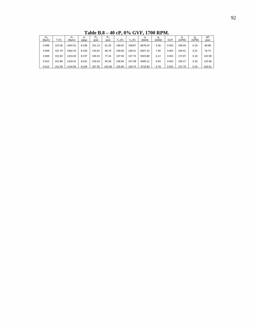
92
Table B.8 – 40 cP, 0% GVF, 1700 RPM. mg
(lbpm) T (F) ml
(lbpm) ρl
(ppg) PD
(psi) PS
(psi) TS (F) TD (F) ql
(bbl/d) qg
(bbl/d) GVF ql
(GPM) qg
(GPM) ΔP
(psi)
0.008 102.36 1604.01 8.236 151.13 81.25 108.62 108.87 6678.24 5.36 0.001 195.00 0.16 69.89
0.009 101.79 1562.43 8.233 143.52 66.79 108.00 108.41 6507.23 7.65 0.001 190.01 0.22 76.73
0.009 101.82 1423.03 8.237 180.43 77.44 107.50 107.74 5923.80 6.12 0.001 172.97 0.18 102.99
0.012 101.88 1318.31 8.241 218.24 94.28 106.84 107.38 5485.12 6.93 0.001 160.17 0.20 123.96
0.013 101.99 1134.55 8.244 267.30 103.38 105.90 106.70 4718.90 6.78 0.001 137.79 0.20 163.91
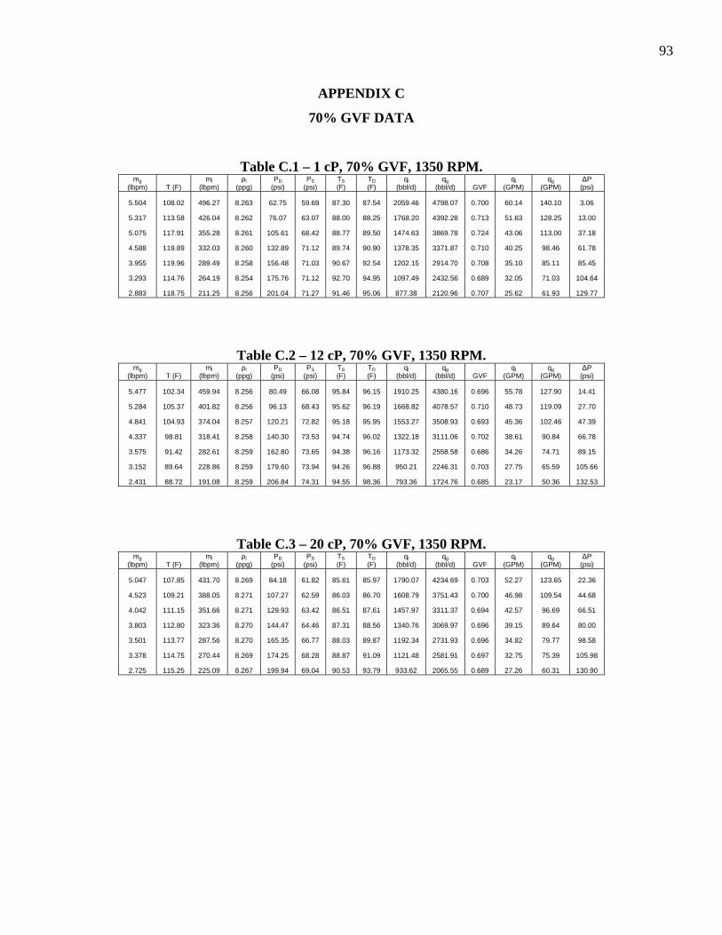
93
APPENDIX C
70% GVF DATA
Table C.1 – 1 cP, 70% GVF, 1350 RPM. mg
(lbpm) T (F) ml
(lbpm) ρl
(ppg) PD
(psi) PS
(psi) TS (F)
TD (F)
ql (bbl/d)
qg (bbl/d) GVF
ql (GPM)
qg (GPM)
ΔP (psi)
5.504 108.02 496.27 8.263 62.75 59.69 87.30 87.54 2059.46 4798.07 0.700 60.14 140.10 3.06
5.317 113.58 426.04 8.262 76.07 63.07 88.00 88.25 1768.20 4392.28 0.713 51.63 128.25 13.00
5.075 117.91 355.28 8.261 105.61 68.42 88.77 89.50 1474.63 3869.78 0.724 43.06 113.00 37.18
4.588 119.89 332.03 8.260 132.89 71.12 89.74 90.90 1378.35 3371.87 0.710 40.25 98.46 61.78
3.955 119.96 289.49 8.258 156.48 71.03 90.67 92.54 1202.15 2914.70 0.708 35.10 85.11 85.45
3.293 114.76 264.19 8.254 175.76 71.12 92.70 94.95 1097.49 2432.56 0.689 32.05 71.03 104.64
2.883 118.75 211.25 8.256 201.04 71.27 91.46 95.06 877.38 2120.96 0.707 25.62 61.93 129.77
Table C.2 – 12 cP, 70% GVF, 1350 RPM. mg
(lbpm) T (F) ml
(lbpm) ρl
(ppg) PD
(psi) PS
(psi) TS (F)
TD (F)
ql (bbl/d)
qg (bbl/d) GVF
ql (GPM)
qg (GPM)
ΔP (psi)
5.477 102.34 459.94 8.256 80.49 66.08 95.84 96.15 1910.25 4380.16 0.696 55.78 127.90 14.41
5.284 105.37 401.82 8.256 96.13 68.43 95.62 96.19 1668.82 4078.57 0.710 48.73 119.09 27.70
4.841 104.93 374.04 8.257 120.21 72.82 95.18 95.95 1553.27 3508.93 0.693 45.36 102.46 47.39
4.337 98.81 318.41 8.258 140.30 73.53 94.74 96.02 1322.18 3111.06 0.702 38.61 90.84 66.78
3.575 91.42 282.61 8.259 162.80 73.65 94.38 96.16 1173.32 2558.58 0.686 34.26 74.71 89.15
3.152 89.64 228.86 8.259 179.60 73.94 94.26 96.88 950.21 2246.31 0.703 27.75 65.59 105.66
2.431 88.72 191.08 8.259 206.84 74.31 94.55 98.36 793.36 1724.76 0.685 23.17 50.36 132.53
Table C.3 – 20 cP, 70% GVF, 1350 RPM. mg
(lbpm) T (F) ml
(lbpm) ρl
(ppg) PD
(psi) PS
(psi) TS (F)
TD (F)
ql (bbl/d)
qg (bbl/d) GVF
ql (GPM)
qg (GPM)
ΔP (psi)
5.047 107.85 431.70 8.269 84.18 61.82 85.61 85.97 1790.07 4234.69 0.703 52.27 123.65 22.36
4.523 109.21 388.05 8.271 107.27 62.59 86.03 86.70 1608.79 3751.43 0.700 46.98 109.54 44.68
4.042 111.15 351.66 8.271 129.93 63.42 86.51 87.61 1457.97 3311.37 0.694 42.57 96.69 66.51
3.803 112.80 323.36 8.270 144.47 64.46 87.31 88.56 1340.76 3069.97 0.696 39.15 89.64 80.00
3.501 113.77 287.56 8.270 165.35 66.77 88.03 89.87 1192.34 2731.93 0.696 34.82 79.77 98.58
3.378 114.75 270.44 8.269 174.25 68.28 88.87 91.09 1121.48 2581.91 0.697 32.75 75.39 105.98
2.725 115.25 225.09 8.267 199.94 69.04 90.53 93.79 933.62 2065.55 0.689 27.26 60.31 130.90

94
Table C.4 – 1 cP, 70% GVF, 1700 RPM. mg
(lbpm) T (F) ml
(lbpm) ρl
(ppg) PD
(psi) PS
(psi) TS (F)
TD (F)
ql (bbl/d)
qg (bbl/d) GVF
ql (GPM)
qg (GPM)
ΔP (psi)
5.823 111.31 549.94 8.247 80.28 55.47 97.18 97.64 2286.54 5560.57 0.709 66.77 162.37 24.81
5.731 112.30 529.04 8.248 92.44 56.74 97.17 97.81 2199.46 5350.50 0.709 64.22 156.23 35.70
5.549 113.01 536.61 8.248 106.63 58.24 97.03 97.74 2230.95 5045.40 0.693 65.14 147.33 48.39
5.443 113.40 510.40 8.247 123.51 59.54 96.70 97.64 2122.07 4837.74 0.695 61.96 141.26 63.97
5.054 112.37 469.98 8.249 159.65 61.53 96.25 97.79 1953.67 4343.72 0.690 57.05 126.84 98.12
4.867 111.08 426.76 8.249 185.20 63.45 95.68 97.67 1774.01 4051.99 0.695 51.80 118.32 121.75
4.824 110.54 388.19 8.250 198.37 64.10 95.19 97.63 1613.53 3972.35 0.711 47.12 115.99 134.26
Table C.5 – 12 cP, 70% GVF, 1700 RPM. mg
(lbpm) T (F) ml
(lbpm) ρl
(ppg) PD
(psi) PS
(psi) TS (F)
TD (F)
ql (bbl/d)
qg (bbl/d) GVF
ql (GPM)
qg (GPM)
ΔP (psi)
5.977 99.15 577.96 8.254 79.33 56.20 96.22 96.60 2401.04 5623.97 0.701 70.11 164.22 23.13
5.724 101.37 532.79 8.255 102.29 58.96 96.39 97.07 2213.23 5135.68 0.699 64.63 149.96 43.33
5.627 100.91 516.46 8.254 110.70 59.90 96.45 97.21 2145.49 4969.47 0.698 62.65 145.11 50.80
5.387 97.91 467.54 8.254 131.98 61.75 96.40 97.42 1942.26 4614.36 0.704 56.71 134.74 70.23
5.049 94.24 420.22 8.256 159.67 64.09 95.87 97.50 1745.44 4163.29 0.705 50.97 121.57 95.58
4.956 96.07 397.44 8.255 169.36 65.25 96.02 97.93 1650.92 4014.63 0.708 48.21 117.23 104.11
4.320 90.76 351.28 8.256 196.90 66.32 95.34 97.94 1458.98 3439.33 0.702 42.60 100.43 130.59
Table C.6 – 20 cP, 70% GVF, 1700 RPM. mg
(lbpm) T (F) ml
(lbpm) ρl
(ppg) PD
(psi) PS
(psi) TS (F)
TD (F)
ql (bbl/d)
qg (bbl/d) GVF
ql (GPM)
qg (GPM)
ΔP (psi)
5.793 114.01 561.20 8.253 83.09 55.52 97.80 98.31 2331.82 5532.46 0.703 68.09 161.55 27.57
5.682 114.05 549.81 8.253 97.73 57.68 97.63 98.27 2284.33 5222.09 0.696 66.70 152.49 40.05
5.601 113.16 514.03 8.254 110.63 58.80 97.31 98.22 2135.56 5046.34 0.703 62.36 147.35 51.83
5.477 113.20 496.70 8.254 120.49 59.57 97.18 98.15 2063.36 4870.03 0.702 60.25 142.20 60.92
5.243 114.16 452.22 8.256 141.53 61.02 96.74 98.03 1878.23 4548.07 0.708 54.84 132.80 80.52
5.252 113.14 423.10 8.257 150.68 61.72 96.21 97.64 1757.03 4499.59 0.719 51.31 131.39 88.96
4.700 113.20 415.07 8.258 178.25 62.81 95.33 97.29 1723.55 3950.95 0.696 50.33 115.37 115.45
4.395 113.39 393.16 8.260 198.19 64.08 94.25 96.70 1632.19 3614.42 0.689 47.66 105.54 134.11
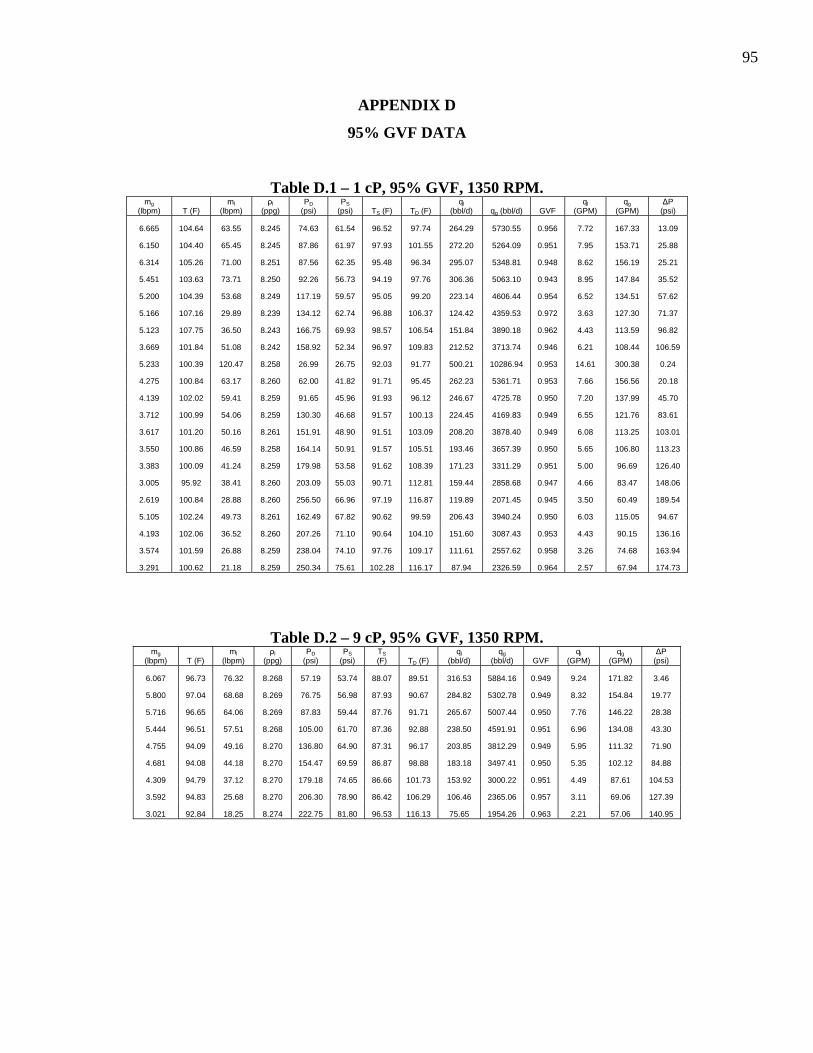
95
APPENDIX D
95% GVF DATA
Table D.1 – 1 cP, 95% GVF, 1350 RPM. mg
(lbpm) T (F) ml
(lbpm) ρl
(ppg) PD
(psi) PS
(psi) TS (F) TD (F) ql
(bbl/d) qg (bbl/d) GVF ql
(GPM) qg
(GPM) ΔP
(psi)
6.665 104.64 63.55 8.245 74.63 61.54 96.52 97.74 264.29 5730.55 0.956 7.72 167.33 13.09
6.150 104.40 65.45 8.245 87.86 61.97 97.93 101.55 272.20 5264.09 0.951 7.95 153.71 25.88
6.314 105.26 71.00 8.251 87.56 62.35 95.48 96.34 295.07 5348.81 0.948 8.62 156.19 25.21
5.451 103.63 73.71 8.250 92.26 56.73 94.19 97.76 306.36 5063.10 0.943 8.95 147.84 35.52
5.200 104.39 53.68 8.249 117.19 59.57 95.05 99.20 223.14 4606.44 0.954 6.52 134.51 57.62
5.166 107.16 29.89 8.239 134.12 62.74 96.88 106.37 124.42 4359.53 0.972 3.63 127.30 71.37
5.123 107.75 36.50 8.243 166.75 69.93 98.57 106.54 151.84 3890.18 0.962 4.43 113.59 96.82
3.669 101.84 51.08 8.242 158.92 52.34 96.97 109.83 212.52 3713.74 0.946 6.21 108.44 106.59
5.233 100.39 120.47 8.258 26.99 26.75 92.03 91.77 500.21 10286.94 0.953 14.61 300.38 0.24
4.275 100.84 63.17 8.260 62.00 41.82 91.71 95.45 262.23 5361.71 0.953 7.66 156.56 20.18
4.139 102.02 59.41 8.259 91.65 45.96 91.93 96.12 246.67 4725.78 0.950 7.20 137.99 45.70
3.712 100.99 54.06 8.259 130.30 46.68 91.57 100.13 224.45 4169.83 0.949 6.55 121.76 83.61
3.617 101.20 50.16 8.261 151.91 48.90 91.51 103.09 208.20 3878.40 0.949 6.08 113.25 103.01
3.550 100.86 46.59 8.258 164.14 50.91 91.57 105.51 193.46 3657.39 0.950 5.65 106.80 113.23
3.383 100.09 41.24 8.259 179.98 53.58 91.62 108.39 171.23 3311.29 0.951 5.00 96.69 126.40
3.005 95.92 38.41 8.260 203.09 55.03 90.71 112.81 159.44 2858.68 0.947 4.66 83.47 148.06
2.619 100.84 28.88 8.260 256.50 66.96 97.19 116.87 119.89 2071.45 0.945 3.50 60.49 189.54
5.105 102.24 49.73 8.261 162.49 67.82 90.62 99.59 206.43 3940.24 0.950 6.03 115.05 94.67
4.193 102.06 36.52 8.260 207.26 71.10 90.64 104.10 151.60 3087.43 0.953 4.43 90.15 136.16
3.574 101.59 26.88 8.259 238.04 74.10 97.76 109.17 111.61 2557.62 0.958 3.26 74.68 163.94
3.291 100.62 21.18 8.259 250.34 75.61 102.28 116.17 87.94 2326.59 0.964 2.57 67.94 174.73
Table D.2 – 9 cP, 95% GVF, 1350 RPM. mg
(lbpm) T (F) ml
(lbpm) ρl
(ppg) PD
(psi) PS
(psi) TS (F) TD (F)
ql (bbl/d)
qg (bbl/d) GVF
ql (GPM)
qg (GPM)
ΔP (psi)
6.067 96.73 76.32 8.268 57.19 53.74 88.07 89.51 316.53 5884.16 0.949 9.24 171.82 3.46
5.800 97.04 68.68 8.269 76.75 56.98 87.93 90.67 284.82 5302.78 0.949 8.32 154.84 19.77
5.716 96.65 64.06 8.269 87.83 59.44 87.76 91.71 265.67 5007.44 0.950 7.76 146.22 28.38
5.444 96.51 57.51 8.268 105.00 61.70 87.36 92.88 238.50 4591.91 0.951 6.96 134.08 43.30
4.755 94.09 49.16 8.270 136.80 64.90 87.31 96.17 203.85 3812.29 0.949 5.95 111.32 71.90
4.681 94.08 44.18 8.270 154.47 69.59 86.87 98.88 183.18 3497.41 0.950 5.35 102.12 84.88
4.309 94.79 37.12 8.270 179.18 74.65 86.66 101.73 153.92 3000.22 0.951 4.49 87.61 104.53
3.592 94.83 25.68 8.270 206.30 78.90 86.42 106.29 106.46 2365.06 0.957 3.11 69.06 127.39
3.021 92.84 18.25 8.274 222.75 81.80 96.53 116.13 75.65 1954.26 0.963 2.21 57.06 140.95
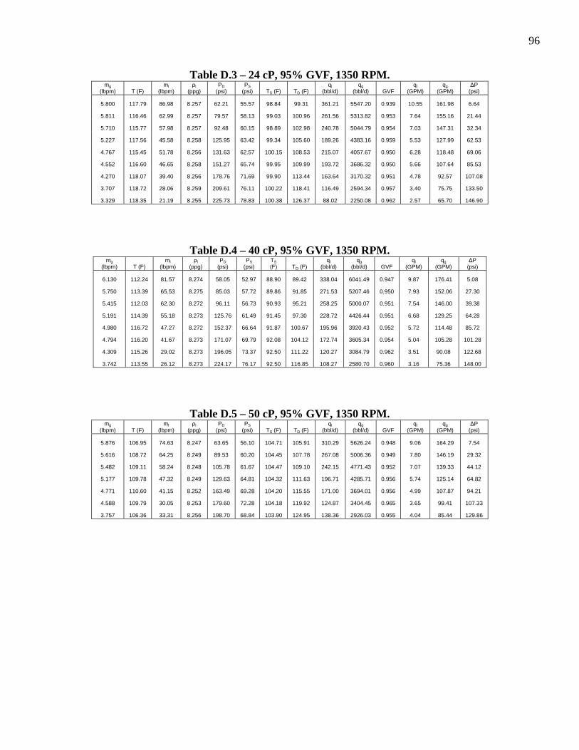
96
Table D.3 – 24 cP, 95% GVF, 1350 RPM. mg
(lbpm) T (F) ml
(lbpm) ρl
(ppg) PD
(psi) PS
(psi) TS (F) TD (F) ql
(bbl/d) qg
(bbl/d) GVF ql
(GPM) qg
(GPM) ΔP
(psi)
5.800 117.79 86.98 8.257 62.21 55.57 98.84 99.31 361.21 5547.20 0.939 10.55 161.98 6.64
5.811 116.46 62.99 8.257 79.57 58.13 99.03 100.96 261.56 5313.82 0.953 7.64 155.16 21.44
5.710 115.77 57.98 8.257 92.48 60.15 98.89 102.98 240.78 5044.79 0.954 7.03 147.31 32.34
5.227 117.56 45.58 8.258 125.95 63.42 99.34 105.60 189.26 4383.16 0.959 5.53 127.99 62.53
4.767 115.45 51.78 8.256 131.63 62.57 100.15 108.53 215.07 4057.67 0.950 6.28 118.48 69.06
4.552 116.60 46.65 8.258 151.27 65.74 99.95 109.99 193.72 3686.32 0.950 5.66 107.64 85.53
4.270 118.07 39.40 8.256 178.76 71.69 99.90 113.44 163.64 3170.32 0.951 4.78 92.57 107.08
3.707 118.72 28.06 8.259 209.61 76.11 100.22 118.41 116.49 2594.34 0.957 3.40 75.75 133.50
3.329 118.35 21.19 8.255 225.73 78.83 100.38 126.37 88.02 2250.08 0.962 2.57 65.70 146.90
Table D.4 – 40 cP, 95% GVF, 1350 RPM. mg
(lbpm) T (F) ml
(lbpm) ρl
(ppg) PD
(psi) PS
(psi) TS (F) TD (F)
ql (bbl/d)
qg (bbl/d) GVF
ql (GPM)
qg (GPM)
ΔP (psi)
6.130 112.24 81.57 8.274 58.05 52.97 88.90 89.42 338.04 6041.49 0.947 9.87 176.41 5.08
5.750 113.39 65.53 8.275 85.03 57.72 89.86 91.85 271.53 5207.46 0.950 7.93 152.06 27.30
5.415 112.03 62.30 8.272 96.11 56.73 90.93 95.21 258.25 5000.07 0.951 7.54 146.00 39.38
5.191 114.39 55.18 8.273 125.76 61.49 91.45 97.30 228.72 4426.44 0.951 6.68 129.25 64.28
4.980 116.72 47.27 8.272 152.37 66.64 91.87 100.67 195.96 3920.43 0.952 5.72 114.48 85.72
4.794 116.20 41.67 8.273 171.07 69.79 92.08 104.12 172.74 3605.34 0.954 5.04 105.28 101.28
4.309 115.26 29.02 8.273 196.05 73.37 92.50 111.22 120.27 3084.79 0.962 3.51 90.08 122.68
3.742 113.55 26.12 8.273 224.17 76.17 92.50 116.85 108.27 2580.70 0.960 3.16 75.36 148.00
Table D.5 – 50 cP, 95% GVF, 1350 RPM. mg
(lbpm) T (F) ml
(lbpm) ρl
(ppg) PD
(psi) PS
(psi) TS (F) TD (F) ql
(bbl/d) qg
(bbl/d) GVF ql
(GPM) qg
(GPM) ΔP
(psi)
5.876 106.95 74.63 8.247 63.65 56.10 104.71 105.91 310.29 5626.24 0.948 9.06 164.29 7.54
5.616 108.72 64.25 8.249 89.53 60.20 104.45 107.78 267.08 5006.36 0.949 7.80 146.19 29.32
5.482 109.11 58.24 8.248 105.78 61.67 104.47 109.10 242.15 4771.43 0.952 7.07 139.33 44.12
5.177 109.78 47.32 8.249 129.63 64.81 104.32 111.63 196.71 4285.71 0.956 5.74 125.14 64.82
4.771 110.60 41.15 8.252 163.49 69.28 104.20 115.55 171.00 3694.01 0.956 4.99 107.87 94.21
4.588 109.79 30.05 8.253 179.60 72.28 104.18 119.92 124.87 3404.45 0.965 3.65 99.41 107.33
3.757 106.36 33.31 8.256 198.70 68.84 103.90 124.95 138.36 2926.03 0.955 4.04 85.44 129.86
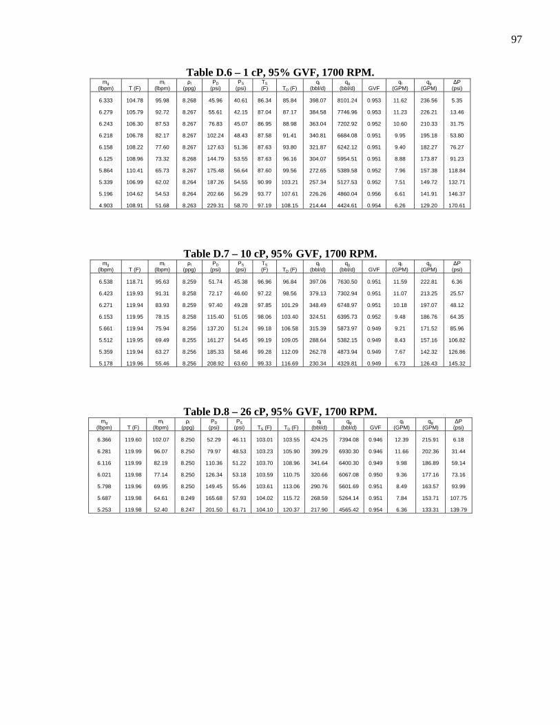
97
Table D.6 – 1 cP, 95% GVF, 1700 RPM. mg
(lbpm) T (F) ml
(lbpm) ρl
(ppg) PD
(psi) PS
(psi) TS (F) TD (F)
ql (bbl/d)
qg (bbl/d) GVF
ql (GPM)
qg (GPM)
ΔP (psi)
6.333 104.78 95.98 8.268 45.96 40.61 86.34 85.84 398.07 8101.24 0.953 11.62 236.56 5.35
6.279 105.79 92.72 8.267 55.61 42.15 87.04 87.17 384.58 7746.96 0.953 11.23 226.21 13.46
6.243 106.30 87.53 8.267 76.83 45.07 86.95 88.98 363.04 7202.92 0.952 10.60 210.33 31.75
6.218 106.78 82.17 8.267 102.24 48.43 87.58 91.41 340.81 6684.08 0.951 9.95 195.18 53.80
6.158 108.22 77.60 8.267 127.63 51.36 87.63 93.80 321.87 6242.12 0.951 9.40 182.27 76.27
6.125 108.96 73.32 8.268 144.79 53.55 87.63 96.16 304.07 5954.51 0.951 8.88 173.87 91.23
5.864 110.41 65.73 8.267 175.48 56.64 87.60 99.56 272.65 5389.58 0.952 7.96 157.38 118.84
5.339 106.99 62.02 8.264 187.26 54.55 90.99 103.21 257.34 5127.53 0.952 7.51 149.72 132.71
5.196 104.62 54.53 8.264 202.66 56.29 93.77 107.61 226.26 4860.04 0.956 6.61 141.91 146.37
4.903 108.91 51.68 8.263 229.31 58.70 97.19 108.15 214.44 4424.61 0.954 6.26 129.20 170.61
Table D.7 – 10 cP, 95% GVF, 1700 RPM. mg
(lbpm) T (F) ml
(lbpm) ρl
(ppg) PD
(psi) PS
(psi) TS (F) TD (F)
ql (bbl/d)
qg (bbl/d) GVF
ql (GPM)
qg (GPM)
ΔP (psi)
6.538 118.71 95.63 8.259 51.74 45.38 96.96 96.84 397.06 7630.50 0.951 11.59 222.81 6.36
6.423 119.93 91.31 8.258 72.17 46.60 97.22 98.56 379.13 7302.94 0.951 11.07 213.25 25.57
6.271 119.94 83.93 8.259 97.40 49.28 97.85 101.29 348.49 6748.97 0.951 10.18 197.07 48.12
6.153 119.95 78.15 8.258 115.40 51.05 98.06 103.40 324.51 6395.73 0.952 9.48 186.76 64.35
5.661 119.94 75.94 8.256 137.20 51.24 99.18 106.58 315.39 5873.97 0.949 9.21 171.52 85.96
5.512 119.95 69.49 8.255 161.27 54.45 99.19 109.05 288.64 5382.15 0.949 8.43 157.16 106.82
5.359 119.94 63.27 8.256 185.33 58.46 99.28 112.09 262.78 4873.94 0.949 7.67 142.32 126.86
5.178 119.96 55.46 8.256 208.92 63.60 99.33 116.69 230.34 4329.81 0.949 6.73 126.43 145.32
Table D.8 – 26 cP, 95% GVF, 1700 RPM. mg
(lbpm) T (F) ml
(lbpm) ρl
(ppg) PD
(psi) PS
(psi) TS (F) TD (F) ql
(bbl/d) qg
(bbl/d) GVF ql
(GPM) qg
(GPM) ΔP
(psi)
6.366 119.60 102.07 8.250 52.29 46.11 103.01 103.55 424.25 7394.08 0.946 12.39 215.91 6.18
6.281 119.99 96.07 8.250 79.97 48.53 103.23 105.90 399.29 6930.30 0.946 11.66 202.36 31.44
6.116 119.99 82.19 8.250 110.36 51.22 103.70 108.96 341.64 6400.30 0.949 9.98 186.89 59.14
6.021 119.98 77.14 8.250 126.34 53.18 103.59 110.75 320.66 6067.08 0.950 9.36 177.16 73.16
5.798 119.96 69.95 8.250 149.45 55.46 103.61 113.06 290.76 5601.69 0.951 8.49 163.57 93.99
5.687 119.98 64.61 8.249 165.68 57.93 104.02 115.72 268.59 5264.14 0.951 7.84 153.71 107.75
5.253 119.98 52.40 8.247 201.50 61.71 104.10 120.37 217.90 4565.42 0.954 6.36 133.31 139.79
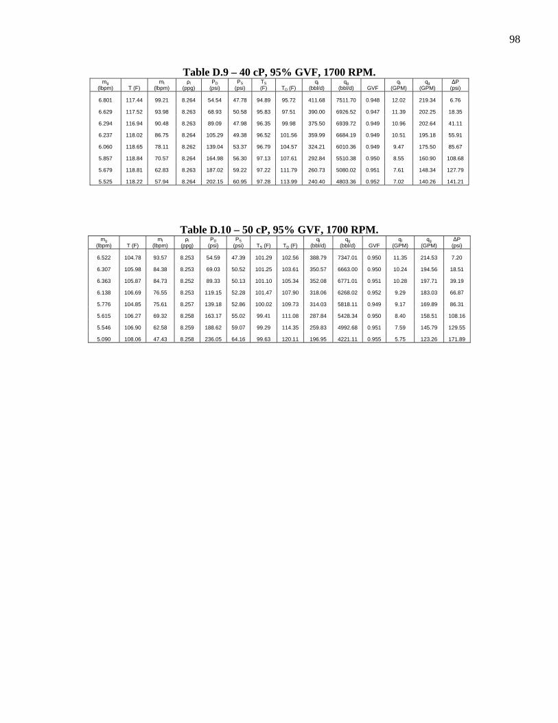
98
Table D.9 – 40 cP, 95% GVF, 1700 RPM. mg
(lbpm) T (F) ml
(lbpm) ρl
(ppg) PD
(psi) PS
(psi) TS (F) TD (F)
ql (bbl/d)
qg (bbl/d) GVF
ql (GPM)
qg (GPM)
ΔP (psi)
6.801 117.44 99.21 8.264 54.54 47.78 94.89 95.72 411.68 7511.70 0.948 12.02 219.34 6.76
6.629 117.52 93.98 8.263 68.93 50.58 95.83 97.51 390.00 6926.52 0.947 11.39 202.25 18.35
6.294 116.94 90.48 8.263 89.09 47.98 96.35 99.98 375.50 6939.72 0.949 10.96 202.64 41.11
6.237 118.02 86.75 8.264 105.29 49.38 96.52 101.56 359.99 6684.19 0.949 10.51 195.18 55.91
6.060 118.65 78.11 8.262 139.04 53.37 96.79 104.57 324.21 6010.36 0.949 9.47 175.50 85.67
5.857 118.84 70.57 8.264 164.98 56.30 97.13 107.61 292.84 5510.38 0.950 8.55 160.90 108.68
5.679 118.81 62.83 8.263 187.02 59.22 97.22 111.79 260.73 5080.02 0.951 7.61 148.34 127.79
5.525 118.22 57.94 8.264 202.15 60.95 97.28 113.99 240.40 4803.36 0.952 7.02 140.26 141.21
Table D.10 – 50 cP, 95% GVF, 1700 RPM. mg
(lbpm) T (F) ml
(lbpm) ρl
(ppg) PD
(psi) PS
(psi) TS (F) TD (F) ql
(bbl/d) qg
(bbl/d) GVF ql
(GPM) qg
(GPM) ΔP
(psi)
6.522 104.78 93.57 8.253 54.59 47.39 101.29 102.56 388.79 7347.01 0.950 11.35 214.53 7.20
6.307 105.98 84.38 8.253 69.03 50.52 101.25 103.61 350.57 6663.00 0.950 10.24 194.56 18.51
6.363 105.87 84.73 8.252 89.33 50.13 101.10 105.34 352.08 6771.01 0.951 10.28 197.71 39.19
6.138 106.69 76.55 8.253 119.15 52.28 101.47 107.90 318.06 6268.02 0.952 9.29 183.03 66.87
5.776 104.85 75.61 8.257 139.18 52.86 100.02 109.73 314.03 5818.11 0.949 9.17 169.89 86.31
5.615 106.27 69.32 8.258 163.17 55.02 99.41 111.08 287.84 5428.34 0.950 8.40 158.51 108.16
5.546 106.90 62.58 8.259 188.62 59.07 99.29 114.35 259.83 4992.68 0.951 7.59 145.79 129.55
5.090 108.06 47.43 8.258 236.05 64.16 99.63 120.11 196.95 4221.11 0.955 5.75 123.26 171.89

99
APPENDIX E
100% GVF DATA
Table E.1 – 1 cp, 100% GVF, 1350 RPM. mg
(lbpm) T (F) ml
(lbpm) ρl
(ppg) PD
(psi) PS
(psi) TS (F) TD (F)
ql (bbl/d)
qg (bbl/d) GVF
ql (GPM)
qg (GPM)
ΔP (psi)
6.628 102.89 2.52 8.252 68.30 60.38 95.51 98.09 10.47 5797.58 0.998 0.31 169.29 7.91
4.113 110.39 2.67 8.253 91.05 73.50 97.20 101.09 11.10 2966.00 0.996 0.32 86.61 17.55
3.449 94.71 4.18 8.260 179.62 54.08 90.06 117.78 17.36 3338.30 0.995 0.51 97.48 125.54
5.718 99.11 3.19 8.277 76.80 53.55 81.90 86.94 13.21 5501.93 0.998 0.39 160.66 23.26
5.220 100.50 3.00 8.274 93.26 53.37 84.00 95.67 12.42 5058.60 0.998 0.36 147.71 39.90
5.097 101.62 2.57 8.271 110.98 56.61 85.42 104.60 10.65 4668.51 0.998 0.31 136.32 54.37
4.718 103.27 2.90 8.272 139.42 58.71 86.54 112.25 12.02 4175.20 0.997 0.35 121.92 80.71
5.977 101.81 2.96 8.260 67.62 52.91 91.12 96.94 12.28 5918.55 0.998 0.36 172.82 14.70
5.753 103.34 2.74 8.259 100.50 59.78 91.93 100.68 11.40 5049.55 0.998 0.33 147.45 40.72
5.065 103.44 2.87 8.259 161.94 68.20 92.27 108.78 11.94 3899.91 0.997 0.35 113.88 93.74
4.074 103.35 2.92 8.259 191.91 72.04 92.08 118.37 12.11 2968.24 0.996 0.35 86.67 119.87
3.202 102.76 2.96 8.259 211.10 75.86 92.29 128.65 12.31 2216.53 0.994 0.36 64.72 135.24
Table E.2 – 9 cp, 100% GVF, 1350 RPM. mg
(lbpm) T (F) ml
(lbpm) ρl
(ppg) PD
(psi) PS
(psi) TS (F) TD (F)
ql (bbl/d)
qg (bbl/d) GVF
ql (GPM)
qg (GPM)
ΔP (psi)
6.487 94.11 3.78 8.269 79.15 61.13 87.55 94.75 15.67 5524.77 0.997 0.46 161.32 18.02
6.177 95.37 3.80 8.270 95.59 64.23 87.66 97.76 15.76 5007.73 0.997 0.46 146.23 31.36
5.766 96.55 3.57 8.270 118.53 67.56 87.68 102.48 14.82 4444.14 0.997 0.43 129.77 50.97
4.852 98.10 3.76 8.271 141.69 75.11 87.77 107.91 15.58 3363.91 0.995 0.46 98.23 66.57
4.865 90.50 3.71 8.268 133.54 62.41 86.44 102.63 15.40 4050.70 0.996 0.45 118.28 71.13
3.641 92.91 3.94 8.270 208.34 78.37 86.94 113.34 16.32 2417.01 0.993 0.48 70.58 129.97
0.744 90.82 3.64 8.270 246.88 89.39 87.12 125.89 15.09 432.75 0.966 0.44 12.64 157.49

100
VITA
Evan Chan 3907 Flintrock Ln. Sugar Land, Texas 77479 Phone: (281) 980-6038 Email: [email protected] Education
Texas A&M University, College Station, Texas Master of Science, Petroleum Engineering, August 2006 GPA: 3.84/4.00
Brown University, Providence, Rhode Island Bachelor of Science, Chemical Engineering, 2004