Embed Size (px)
Citation preview

WELDING RESEARCH
MARCH 2004-S82
ABSTRACT. This work describes the detailed derivation of theanalytical approximate solution for a double ellipsoidal densityheat source in finite thick plate. This has shown that the solutionof the heat source can be effectively used to predict the thermalhistory of the thick welded plate as well as weld pool shape geom-etry and various welding simulation purposes once the parame-ters of the heat source have been calibrated. This approximate so-lution can be directly used for welding simulation of finite thickplate without the need for implementing the mirror method as re-quired in a semi-infinite body. Hence, it can be used as a poten-tially convenient tool for solving many problems in thermal stressanalysis, residual stress analysis, and microstructure modeling ofmultipass welds, and others.
Introduction
The temperature history of welded components has a signifi-cant influence on the residual stresses, distortion, and hence thefatigue behavior of welded structures. In order to obtain a goodprediction for residual stress and distortion in welded joints andstructures, an appropriate heat source is needed for that purpose.
Goldak et al. (Ref. 1) first introduced a three-dimensional (3-D) double ellipsoidal moving heat source and used finite elementmethod (FEM) to calculate the temperature field of a bead onplate. He had shown that the 3-D heat source could overcome theshortcomings of the previous 2-D Gaussian model in order to pre-dict the temperature of the welded joints with much deeper pen-etration. Nguyen et al. (Ref. 2) has recently developed a closedform analytical solution for this kind of 3-D heat source in a semi-infinite body and showed that this solution can be used for weldpool geometry prediction (Ref. 2) and for the calculation of resid-ual stresses in a bead-on-plate weld (Ref. 3). However, the recentheat source solution is still limited to the semi-infinite body andone has to use the mirror image method when applying the solu-tion for finite plates. This makes implementation of the solutiona tedious task, especially for some complicated geometries.
In this paper, an analytical approximate solution for double el-lipsoidal heat source in finite thick plate has been derived and cal-ibrated with the experimental data.
Theoretical Analysis
Temperature Field Solution Based on Green’s Function forInstantaneous Point Source
Let us consider heat quantity δQ(x', y', z', t') acting instanta-neously at time t' at point (x',y',z') in infinite body. The infinitesi-mal rise in temperature due to this point heat source dT(x,y,z,t') atpoint (x,y,z) and time t' in infinite body has been well established(Ref. 4) as
where dT(x,y,z,t') is an infinitesimal rise in temperature due to thepoint heat source δQ(x',y',z',t'), ρ and c are mass density and spe-cific heat, k is heat conduction coefficient, and a is thermal diffu-sivity (a = k/cρ).
Subsequently, the temperature field T(x,y,z,t) at time t for thispoint heat source δQ(x',y',z',t') can be obtained as
where To is the initial temperature; Ginf(x,y,z,t;x',y',z',t') is theGreen’s function solution for the point source of unit magnitudein the infinite body, which is the temperature at point (x,y,z) andtime t due to the instantaneous point source located at (x',y',z') attime t' and obtained as the solution to the heat conduction equa-tion (∂T/∂t = a∇2T) as
Based on Equation 2, the temperature field for any kind of heatsource [line heat source (1-D), surface heat source (2-D), or vol-ume heat source (3-D)] in infinite body can be obtained by carry-
G x y z t x y z t dt
a t t
x x y y z z
a t t
inf ( , , , ; ' , ' , ' , ' ) '
( ' )
( ' ) ( ' ) ( ' )
( ' )
=
−[ ]• − + − + −
−
1
4
exp4
(3)
3/ 2
2 2 2
π
T x y z t TQ x y z t
c
G x y z t x y z t dt
o
t
( , , , )( ' , ' , ' , ' )
( , , , ; ' , ' , ' , ' ) 'inf
− =
•
∫ δρ
0
(2)
dT x y z tQ x y z t dt
c a t t
x x y y z z
a t t
( , , , ' )( ' , ' , ' , ' ) '
( ' )
( ' ) ( ' ) ( ' )
( ' )
= •−
• − − + − + −−
δρ π[4 ]
exp4
(1)
3/ 2
2 2 2
KEY WORDS
Double Ellipsoidal Heat SourceSingle Ellipsoidal Heat SourceGas Metal Arc WeldingFinite BodySemi-Infinite BodyAnalytical Approximate Solution
Analytical Approximate Solution for DoubleEllipsoidal Heat Source in Finite Thick Plate
Analytical approximate solutions for double ellipsoidal heat sources in finite thickplate have been derived and calibrated with the experimental data
BY N. T. NGUYEN, Y.-W. MAI, S. SIMPSON, AND A. OHTA
N. T. NGUYEN is with ETRS Pty Ltd., Mulgrave, Australia. Y.-W. MAI is with Center for Advanced Materials & Technology (CAMT), School of Aerospace,Mechanical & Mechatronic Engineering, and S. SIMPSON is with School of Electrical and Information Engineering, The University of Sydney, Australia. A.OHTA is with Materials Strength and Life Evaluation Station, National Research Institute for Metals, Japan.

WELDING RESEARCH
-S83WELDING JOURNAL
ing out the corresponding line, surface, or volume integration. Fora volume distributed heat source with heat density Q(x',y',z',t') thetemperature field in infinite body would be
Note that this solution is based on Green’s function for a pointheat source in an infinite body. If a volume heat source in a finitebody is considered, a new Green’s function for a point heat sourcein the finite body that satisfies the Neumann boundary conditionof zero heat density (∂T/∂n = 0 where n is the normal direction)across its boundary surfaces should be adopted as
where Gfin(x,y,z,t;x',y',z',t') is the Green’s function for point heatsource in finite body.
Approximate Approach for Temperature Field Subjected to Volume Heat Source in Finite Body
It can be seen from Equation 5 that exact solutions for variouskinds of heat sources in a finite body can be obtained if the Green’sfunction for the point heat source in that particular body is known.However, the Green’s function for the point heat source in a finitebody would be expressed in a much more complicated form thanthat in an infinite body. Therefore, finding an analytical solutionfor Equation 5 would become an almost impossible task.
An alternative approximate approach to compensate for theNeumann boundary condition when dealing with a finite body isto keep using the same Green’s function for the point source in aninfinite body but replacing the heat source in an infinite body bythe effective heat source Qeff(x',y',x',t') in the finite body. The ef-fective heat source should produce the same amount of heat inputinto the finite body as the original heat source would in an infinitebody. This means that the amount of heat transferred in the wholeinfinite body now would rather be contained only in the finite
body. Subsequently, Equation 5 becomes
This approximate approach based on Equation 6 is reasonableas it is based on the two following assumptions:
1) The principle of conservation of energy for total heat inputin infinite and finite bodies.
2) There is an insignificant effect of Green’s functions for apoint heat source in infinite and finite bodies on the shape of thedistribution of the temperature field.
An example of deriving the exact conduction-only solution andapproximate solution for the single ellipsoidal heat source in asemi-infinite body based on the above analysis is given in Appen-dix A. It has been shown that the Green’s functions for point heatsource in a semi-infinite body and a finite body do not change theshape of the temperature field, i.e., assumption 2 is correct in thecase of a semi-infinite body.
Therefore, in this paper, this approximate approach has beenimplemented to obtain the analytical solution for a double ellip-soidal heat source in finite thick plate based on Equation 6.
Ellipsoidal Heat Sources and Their ApproximateSolution for Finite Plate
Goldak’s Ellipsoidal Heat Sources in Semi-Infinite Body
Single Ellipsoidal Heat Source
Goldak et. al. (Ref. 1) initially proposed a semi-ellipsoidal heatsource in which heat density is distributed in a Gaussian mannerthroughout the heat source’s volume. The heat density Q(x,y,z) ata point (x,y,z) within the semi-ellipsoid is given by the followingequation:
Q x y zV I
a b c
x
c
y
a
z
bh h h h h h
( , , ) =• •
− − −
6 3exp
3 3 3(7)
2 2
2
2
2 2
η
π π
T x y z t TQ x
G x y z t x y z t dx dy dz dt
oeff
t
V
( , , , )
( , , , ; ' , ' , ' , ' ) ' ' ' 'inf
− =
•
∫∫∫∫( ' , y' z' , t' )
c
(6)0
ρ
T x y z t TQ x y z t
c
G x y z t x y z t dx dy dz dt
o
t
V
fin
( , , , )
( , , , ; ' , ' , ' , ' ) ' ' ' '
− =
•
∫∫∫∫( ' , ' , ' , ' )
(5)0
ρ
T x y z t TQ x y z t
c
G x y z t x y z t dx dy dz dt
o
t
V
( , , , )
( , , , ; ' , ' , ' , ' ) ' ' ' 'inf
− =
•
∫∫∫∫( ' , ' , ' , ' )
(4)0
ρ
Fig. 1 — Double ellipsoidal power density distributed heat source. Fig. 2 — Single ellipsoidal heat source in a finite thick plate.
WELDING RESEARCH
MARCH 2004-S84
where ah, bh, and ch are ellipsoidal heat source parameters as de-scribed in Fig. 1 (chf = chb= ch); x,y,z are moving coordinates ofthe heat source; Q(x,y,z) is heat density at a point (x,y,z); V and Iare welding voltage and current, respectively, and η is arc effi-ciency.
Goldak’s Double Ellipsoidal Heat Source
Practical experience with the single heat source showed thatthe predicted temperature gradients in front of the arc were lesssteep than the experimentally observed ones, and gradients be-hind the arc were steeper than those measured. To overcome this,two ellipsoids were combined and proposed as a new heat sourcecalled “double ellipsoidal heat source” as shown in Fig. 1 (Ref. 1).
Since two different semi-ellipsoids are combined to give thenew heat source, the heat density within each semi-ellipsoid aredescribed by different equations. For a point (x,y,z) within the firstsemi-ellipsoid located in front of the welding arc, the heat densityequation is described as
and for points (x,y,z) within the second semi-ellipsoid covering therear section of the arc as
where ah, bh, chf, and chb are ellipsoidal heat source parameters asdescribed in Fig. 1, Q is the heat input (Q = ηIV), rf and rb are pro-portion coefficients representing heat apportionment in front andback of the heat source, respectively (rf + rb = 2).
It must be noted here that due to the continuity of the volu-metric heat source, the values of Q(x,y,z) given by Equations 8 and9 must be equal at the x = 0 plane. From that condition, anotherconstraint is obtained for rf and rb as rf/chf = rb/chb. Subsequently,the values for these two coefficients are determined as rf =2chf/(chf + chb); rb = 2chb/(chf + chb).
It is also worth noting here that this double ellipsoidal distrib-
ution heat source is described by five unknown parameters: thearc efficiency η and four ellipsoidal axes parameters, ab, bb, chf,and chb. Goldak et al. (Ref. 1) implied there is equivalence be-tween the source dimensions and those of the weld pool and sug-gested that appropriate values for ab, bb, chf, and cbf could be ob-tained by direct measurement of weld geometry.
Effective Single Ellipsoidal Heat Sources in Finite Thick Plate
Single Ellipsoidal Heat Sources in Finite Thick Plate
Let us consider a single ellipsoidal heat source in a finite plateof width 2B, length 2L, and thickness D. The local coordinate ofthe heat source (O'x'y'z') is constructed so that its axes are paral-lel to the fixed coordinate of the finite plate (Oxyz) as shown inFig. 2 where origin O' is located at O'(x,y,z).
Based on Goldak’s heat source in a semi-infinite body, the sin-gle ellipsoidal heat source in finite plate is assumed to have thesimilar form but deferent maximum heat density magnitude as
Furthermore, assuming that heat convection and radiation are ig-norable due to the short time of welding in a quiet air environ-ment, the conservation of energy in the finite plate requires that
or
Equation 11B can be further simplified using the error functiondefinition and rearranged for Qmax as
Q Qx
cdx
y
ady
z
bdz
hL x
L x
hB y
B y D
h
= −
• −
−
− −
−
− −
−
∫
∫ ∫
max'
'
''
''
exp3
exp3
exp3
(11B)
2
2
2
20
2
21
2 2 exp3 3 3
(11A)2
2
2
2
2
20
Q Qx
c
y
a
z
bdx dy dz
h h h
D
B y
B y
L x
L x
= − − −
∫∫∫
− −
−
− −
−
max' ' '
' ' '
Q x y z Qx
c
y
a
z
beff
h h h
( ' , ' , ' )' ' '
max= − − −
exp3 3 3
(10)2
2
2
2
2
2
Q x y zr Q
a b c
x
c
y
a
z
b
b
h h hb hb h
( , , ) = − − −
6 3exp
3 3 3(9)
2
2
2
2
2
h2π π
Q x y zr Q
a b c
x
c
y
a
z
b
f
h h hf hf h h
( , , ) = − − −
6 3
π πexp
3 3 3(8)
2
2 2
2
2
2
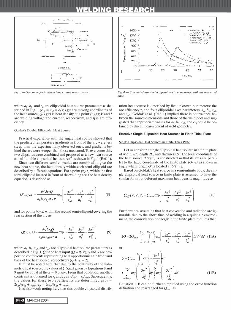
Fig. 4 — Calculated transient temperatures in comparison with the measuredones.
Fig. 3 — Specimen for transient temperature measurement.

WELDING RESEARCH
-S85WELDING JOURNAL
Substituting Equation 12 into Equation 10 gives the heat densityequation for the proposed single ellipsoidal heat source in the fi-nite plate as
Analytical Approximate Solution for Single Ellipsoidal Heat Sourcein Finite Thick Plate
Let us consider a finite plate of width 2B, length 2L, and thick-ness D as in Fig. 2 again. The approximate solution for the singleellipsoidal heat source in this finite thick plate is based on the ap-proach described in the section titled “Approximate Approach forTemperature Field Subjected to Volume Heat Source in FiniteBody.” Substituting Equations 3 and 10 into Equation 5 and re-arranging the variables gives
or
where
T x y z t TQ dt
c a t t
I I Io
t
L B D( , , , )'
( ' )
max− =
−[ ]∫
ρ π4
(14B)3/ 2
0
T x y z t TQ dt
c a t t
x
c
x x
a t tdx
y
a
y y
a t t
o
t
hL x
L x
hB
( , , , )'
( ' )
' ( ' )
( ' )'
' ( ' )
( ' )
max− =
−[ ]− − −
−
• − − −−
∫ ∫− −
−
− −
ρ π4
exp3
4
exp3
4
3/ 20
2
2
2
2 2
2yy
B y D
h
dyz
b
z z
a t tdz
−
∫ ∫⋅ − − −−
'' ( ' )
( ' )'exp
3
4(14A)
0
2
2
2
Q x y z
Qx
c
y
a
z
b
a b cD
c
L x
c
L x
c
effh h h
h h hh
h h
' , ' , '
' ' '
( ) =
− − −
•−( )
++( )
24 3exp3 3 3
erf3
erf3
erf3
2
2
2
2
2
2
π π
•−( )
++( )
erf3
erf3
(13)
B y
a
B y
ah h
a b c erfD
c
L x
c
L x
c
B y
a
B y
a
h h hh
h h
h h
max =
•−( )
++( )
•−( )
++( )
24 3
3
erf3
erf3
erf3
erf3
π π
(12)
Fig. 5 — Effect of ah on the weld pool geometry. A — Top view of the weld pool;B — longitudinal cross section of the weld pool.
Fig. 6 — Effect of bh on the weld pool geometry. A — Top view of the weld pool;B — longitudinal cross section of the weld pool.
A
B
A
A
B
B
Fig. 7 — Effect of chf on the weld pool geometry. A — Top view of the weldpool; B — longitudinal cross section of the weld pool.

WELDING RESEARCH
MARCH 2004-S86
Integrals IL, IB, and ID can be solved using the error function no-tation as
Substituting Equations 12 and 15A–C into Equation 14B and sub-sequently simplifying gives
where
E L x c
a t t c L x c x
c a t t a t t c
a t t c L x c x
c a t t a t t c
h
h h
h h
h h
h( , , )
( ' ) ( )
( ' ) ( ' )
( ' ) ( )
( ' ) ( ' )=
− +
− −
− − +
+− +
+ −
− − +
erf12
4 12
erf12
4 12
2 2
2
2 2
hh
h h
L x
c
L x
c
2
erf3
erf3
(16B)
−
+ +
( ) ( )
T x y z t TQ
c
E L x c E B y a E D z b
a t t a a t t b a t t c
x
a t t c
y
a t
o
h h h
h h h
t
h
( , , , )
( , , ) ( , , ) ( , , )
( ' ) ( ' ) ( ' )
( ' ) (
− =
• • •
− + − + − +
• −− +
−−
∫
3 3
12 12 12
exp3
12
3
12
2 2 2
2
2
2
ρ π π
0
tt a
z
a t t bdt
h h' ) ( ' )'
+−
− +
2
2
2
3
12 (16A)
Iz
a t t b
b a t t
a t t b
a t t D b D z
b a t t a t t b
b z
a t t a
Dh
h
h
h
h h
h
= −− +
•
−
− +
•
− + −
− − +
+−
exp3
12
4
12
2
erf12
4 12
erf4 12
2
2 2
2
2
( ' )
( ' )
( ' )
( ' ) ( )
( ' ) ( ' )
( ' ) (
π
tt t bh− +
' ) 2
(15C)
Iy
a t t a
a a t t
a t t a
a t t a B y a y
a a t t a t t a
a t t
Bh
h
h
h h
h h
= −− +
•
−
− +
•
− +( ) − −
− − +
+−
exp3
12
4
12
2
erf12
4 12
erf12
2
2 2
2 2
2
( ' )
( ' )
( ' )
( ' ) ( )
( ' ) ( ' )
( ' )
π
++( ) + −
− − +
a B y a y
a a t t a t t a
h h
h h
2 2
24 12
(15B)( )
( ' ) ( ' )
Ix
a t t c
c a t t
a t t c
a t t c L x c x
c a t t a t t c
a t t
Lh
h
h
h h
h h
= −− +
•
−
− +
•
− +( ) − −
− − +
+−
exp12
4
12
2
erf12
4 12
erf12
2
2 2
2 2
2
3
( ' )
( ' )
( ' )
( ' ) ( )
( ' ) ( ' )
( ' )
π
++( ) + −
− − +
c L x c x
c a t t a t t c
h h
h h
2 2
24 12
(15A)( )
( ' ) ( ' )
Ix
c
x x
a t tdx
Iy
a
y y
a t tdy
Iz
b
z z
a t
L
hL x
L x
B
hB y
B y
D
h
= − − −−
= − − −−
= − − −−
− −
−
− −
−
∫
∫
exp3
4
exp3
4
exp3
4
2
2
2
2
2
2
2
' ( ' )
( ' )'
' ( ' )
( ' )'
' ( ' )
(
2
2
ttdz
D
')'
∫
0
Fig. 8 — Experimental setup for specimen fabrication and data acquisition. A — Welding system for specimen fabrication; B — data logging system usingWeldPrint software.
A B

WELDING RESEARCH
-S87WELDING JOURNAL
Finally, substituting x = x – vt' (for the moving heat source withconstant speed v in x-direction) to Equations 16A and B gives thefinal approximate solution for the moving heat source in a finitethick plate as
It is worth noting here that the approximate solution obtainedfor the moving single ellipsoidal heat source in finite plate as givenby Equation 17 is of the similar form as that obtained earlier byNguyen et al. (Ref. 2) for the heat source in semi-infinite body, ex-cept for the error function correction terms [E(L, x–vt'), E(B,y),and E(D,z)] due to plate length, width, and thickness, respectively.
Effective Double Ellipsoidal Heat Sources in Finite Plate
Double Ellipsoidal Heat Sources in Finite PlateLet us now consider that the heat source consists of two quar-
ters of different ellipsoids as shown in Fig. 1. Following a similarprocedure as described in the previous section for the single el-lipsoidal heat source, density equations are obtained for the frontand back half of the double ellipsoidal heat source, respectively asfollows
Q x y z
Qrx
c
y
a
z
b
a b cD
b
L x
c
L x
c
b eff
b
hb h h
h h hbh
hb hb
, ( ' , ' , ' )
' ' '
( ) ( )
=
− − −
• −
+ +
24 3exp3 3 3
erf3
erf3
erf3
2
2
2
2
2
2
π π
• −
+ +
erf3
erf3
(18B)
( ) ( )B y
a
B y
ah h
Q x y z
Qrx
c
y
a
z
b
a b cD
b
L x
c
L x
c
f eff
f
hf h h
h h hfh
hf hf
, ( ' , ' , ' )
' ' '
( ) ( )
=
− − −
• −
+ +
24 3exp3 3 3
erf3
erf3
erf3
2
2
2
2
2
2
π π
• −
+ +
erf3
erf3
(18A)
( ) ( )B y
a
B y
ah h
T x y z t TQ
c
E L x vt c E B y a E D z b
a t t a t t b a t t c
x vt
a t t c
o
h h h
h h h
t
h
( , , , )
( , ' , ) ( , , ) ( , , )
( ' ) ( ' ) ( ' )
( ' )
( ' )
− =
• − • •
− + − + − +
• − −
− +−
∫
3 3
12 12 12
exp3
12
3
2 2 20
2
2
ρ π π
yy
a t t a
z
a t t bdt
h h
2
2
2
212
3
12 (17)
( ' ) ( ' )'
− +−
− +
E D z b
a t t D b D z
b a t t a t t b
b z
a t t a t t b
h
h
h h
h
h
( , , )
( ' ) ( )
( ' ) ( ' )
( ' ) ( ' )
=
− + −
− − +
+− − +
erf12
4 12
erf4 12
2
2
2
•
−erf3
(16D)1 D
bh
E B y a
a t t a B y a y
a a t t a t t a
a t t a B y a y
a a t t a t t a
h
h h
h h
h h
h( , , )
( ' ) ( )
( ' ) ( ' )
( ' ) ( )
( ' ) ( ' )=
− +
− −
− − +
+− +
+ −
− − +
erf12
4 12
erf12
4 12
2 2
2
2 2
hh
h h
B y
a
B y
a
2
erf3
erf3
(16C)
−
+ +
( ) ( )
Fig. 9 — Comparisons between the measured and the predicted weld poolshape. A — Top view of the weld pool shape; B — transversal cross section ofthe weld pool.
A
B

WELDING RESEARCH
MARCH 2004-S88
where rf and rb are proportion coefficients representing the heatapportionment in front and back of the double ellipsoidal heatsource, respectively, and rf +rb = 2. Applying the continuity con-dition of the volume heat source for the plane x' = 0, the valuesof the heat density given by Equations 18A and B must be equal.Subsequently, the values of rf and rb can be evaluated as
It is worth noting here that this double ellipsoidal heat source forfinite plate is described by five unknown parameters, which arethe arc efficiency coefficient, η, and four other geometric para-meters of the heat source: ah, bh, chf, and chb.
Analytical Approximate Solution for Double Ellipsoidal Heat Source inFinite Thick Plate
An analytical solution for the double ellipsoidal heat source isobtained by substituting heat density Equations 18A and B intoEquation 5 and following a similar procedure as described in thesection titled “Analytical Approximate Solution for Single Ellip-soidal Heat Source in Finite Thick Plate.” The transient temper-
r
cL x
c
L x
c
cL x
c
L x
c
cL x
c
b
hbhb hb
hfhf hf
hbhb
=
• −
+ +
• −
+ +
+ • −
2 erf3
erf3
erf3
erf3
erf3
( ) ( )
( ) ( )
( )
+ +
erf3
(19B)
( )L x
chbr
cL x
c
L x
c
cL x
c
L x
c
cL x
c
f
hfhf hf
hfhf hf
hbhb
=
• −
+ +
• −
+ +
+ • −
2 erf3
erf3
erf3
erf3
erf3
( ) ( )
( ) ( )
( )
+ +
erf3
(19A)
( )L x
chb
Fig. 10 — Macrographs of the welded specimens. A — Weld bead cross section V1B; B — weld bead cross section U2B; C — top view of the weld pool V1B; D— top view of the weld pool U2B
A B
C D

WELDING RESEARCH
-S89WELDING JOURNAL
ature for an arbitrary point (x,y,z) in a finite plate of length 2L,width 2B, and thickness D, subjected to the double ellipsoidal heatsource is given as
where E(L, x–vt', chf), E(L, x–vt', chb), E(B, y, ah), and E(D, z, bh)are given by Equations 16B–D, respectively.
Solution for Ellipsoidal Heat Sources in Dimensionless Form
The solution obtained for single and double ellipsoidal heatsources as shown in Equations 17 and 20 can be expressed furtherin much simpler dimensionless form by introducing the followingdimensionless parameter variables as recommended by Chris-tensen’s method (Ref. 5):• Dimensionless coordinates: ξ = vx/2a, ψ = vy/2a, ζ = vz/2a• Dimensionless time: τ = v2(t–t')/2a• Dimensionless heat source parameters: ua = vah/(2a√6), ub =
vbh/(2a√6), uc = vch/(2a√6), ucf = vchf/(2a√6), and ucb =vchb/(2a√6)
• Dimensionless finite plate parameters: plate length, l = vL/2a;plate width, b = vB/2a, and plate thickness, d = vD/2a
• Dimensionless temperature: θ = (T–To)/(Tc–To) where Tc is thereference temperature
•Christensen’s operating parameter (Ref. 5):n = Qv/(4πa2ρc(Tc–To))Substituting these parameters into Equations 17 and 20 and
simplifying gives the following dimensionless form of the solutionsfor single and double ellipsoidal heat sources in finite plate, re-spectively, as
where l, b, and d are dimensionless length, width, and thickness ofthe plate [l =Lv/(2a√6), b =Bv/(2a√6) and d =Dv/(2a√6)];τmax=v2t/2a and ξ = v2t’/2a are the dimensionless time variables;and e(l, ξ–ξ', ucf), e(l,ξ–ξ', ucb), e(b, ψ, ua),and e(d, ζ, ub) are thecorrection terms for finite plate in dimensionless form as follows:
e b ub
u
b u
u
u
u
b u
u
u
u
a
a
a
a
a
a
a
a
a
a
( , , )ψ
τ
τ
ψ
τ τ
τ
τ
ψ
τ τ
=
•
++
+
++
−+
−erf2
erf2 2
erf2 2
(23C)
1
2
2
2
2
e l ul
u
l u
u
u
u
l u
u
u
u
cb
cb
cb
cb
cb
cb
cb
cb
cb
cb
( , ' , )
( ' )
( ' )
ξ ξ
τ
τ
ξ ξ
τ τ
τ
τ
ξ ξ
τ τ
− =
•
++ −
+
++
− −
+
−erf2
erf2 2
erf2 2
1
2
2
2
2
(23B)
e l ul
u
l u
u
u
u
l u
u
u
u
cf
cf
cf
cf
cf
cf
cf
cf
cf
cf
( , ' , )
( ' )
( ' )
ξ ξ
τ
τ
ξ ξ
τ τ
τ
τ
ξ ξ
τ τ
− =
•
++
−
+
++
−−
+
−erf2
erf2 2
erf2 2
1
2
2
2
2
(23A)
θ
π
ψ ζ
τ τ
ψ
τ
ζ
ττ
ξ ξ ξ ξ
τ
τ
τ
n
e b u e d u
u u
u ud
r e l uu
u
a b
a b
a b
f cf
cf
= •
+ +
• −+
−+
•
− − −
+
+
∫1
2 2
exp2 2
exp2
2 20
2
2
2
2
2
2
( , , ) ( , , )
( ) ( )
( , ' , )( ' )
( )
max
cfcf
b ch
cf
cb
r e l uu
u
2
2
2
2
exp2
(22)
+
− − −
+
+
( , ' , )( ' )
( )ξ ξ ξ ξ
τ
τ
θ
π
ξ ξ ψ ζ
τ τ τ
ξ ξ
τ
ψ
τ
ζ
ττ
τ
n
e l u e b u e d u
u u u
u u ud
c a b
a b c
c a b
= − • •
+ + +
• −
+−
+−
+
∫1
2
exp2 2 2
(21)
2 2 2
2
2
2
2
2
2
( , ' , ) ( , , ) ( , , )
( ' )
( ) ( ) ( )
max
0
T x y z t TQ
c
y
a t t a
z
a t t b
E B y a E D z b
a t t a a t t b
o
h h
h h
h h
( , , , )
( ' ) ( ' )
( , , ) ( , , )
( ' ) ( ' )
− =
−− +
−− +
• •
− + − +
3 3
2
exp3
12
3
12
12 12
2 2
2 2
ρ π π
2 2
•
− − −− +
− +
+− − −
− +
∫0
2
2
2
2
2
exp3
12
12
exp3
12
t
f hfhf
hf
b hbhb
r E L x vt cx vt
a t t c
a t t c
r E L x vt cx vt
a t t c
( , ' , )( ' )
( ' )
( ' )
( , ' , )( ' )
( ' )
− +
•
12
(20)
2a t t c
dt
hb( ' )
'

WELDING RESEARCH
MARCH 2004-S90
and rf and rb become:
Results and Discussion
Numerical Procedure
In this study, a numerical procedure was applied to calculatethe solution for the transient temperature field as described byEquations 16B–D and 20 for the double semi-ellipsoidal distrib-uted heat source. A Fortran77 computer program was written tofacilitate the integral calculation in Equation 20 and to allow forrapid calculation of geometry of the weld pool based on the as-sumed melting temperature of 1520°C for mild steel. Using thisprogram, the effects of various heat source parameters (ah, bh, chf,and chb) on the predicted weld pool geometry were investigated.The following material properties for high-strength steel wereused for the calculation: heat capacity, c = 600 J/kg/°C; thermalconductivity, k = 29 J/m/s/°C; density, ρ = 7820 kg/m3 (Ref. 4).Welding parameters used for calculation are voltage, U = 26 V;current, I = 230 A; welding speed, v = 30 cm/min, and arc effi-ciency, η = 0.8.
Transient Temperature Results
Using the above described numerical procedure, transienttemperatures of three selected points A, B, and C in a square steelplate 240 × 240 × 20 mm (as shown in Fig. 3) have been calculatedand compared with the test results. The parameters of the doubleellipsoids used for the calculation were estimated based on theirrelationship with the weld pool geometry measured after weldingand calibrated with the measured temperature history. The best-fit values of the heat source parameters obtained for these testspecimens are ah = 7 mm, bh = 2 mm, chf = 7 mm, chb = 14 mm.More details about the test specimens and temperature measure-ment are described elsewhere (Ref. 2).
Figure 4 shows a comparison between the calculated transienttemperatures at A, B, and C and the measured ones based on theabove-described heat source parameters, correspondingly. It canbe seen from this figure that the calculated transient temperatures
are in good agreement with those measured in terms of bothtrends and magnitude. The predicted temperatures for weld toepoint A shows steeper slope in cooling cycles compared with thecorresponding measured temperatures. However, for point B theagreement between temperature slopes in the cooling cycles isquite reasonable. The predicted and measured temperatures atpoint C are in excellent agreement and the numerical results alsoshow its kink point due to the corner position of point C as ob-served by the test.
If more sets of calibrated data are available, the relationshipbetween the double ellipsoidal heat source parameters and thewelding parameters such as U, I, v for a particular set of base andwelding materials can be established and used for future heatsource and welding simulation. This means that the approximateanalytical solution for the developed heat source in finite thickplate can be used to simulate the transient temperatures of morecomplicated welding paths once the heat source parameters canbe reliably predicted from the welding parameters for the associ-ated welding materials and welding conditions.
Simulated Weld Pool Results
In this work, a parametric study was carried out for variousgeometric parameters of the heat source to evaluate their influ-ence on the simulated weld pool. Material properties and weldingparameters were the same, as indicated in the section titled“Goldak’s Ellipsoidal Heat Sources in Semi-Infinite Body,” andkept unchanged for all simulations.
Figure 5A and B shows the effect of the heat source parame-ter ah on the top view of the weld pool shape and its longitudinalcross section, respectively, while other heat source parameters arekept unchanged (bh = 2 mm, chf = ah mm, and chb/chf = 2). Fig-ure 5A shows that as ah increases from 1 to 5, the shape of the weldpool becomes shorter and fatter, i.e., its length decreases but itswidth increases. However, as ah increases beyond a certain value(ah > 5 mm), the weld pool becomes shorter and thinner.
This behavior of the heat source can be explained by the na-ture of the distributed heat source. This means that the higher thevalue of ah, the weaker the heat density becomes. At the lower val-ues of ah (ah < 5 mm), when the corresponding heat density is stillhigh enough, the width of the weld pool increases as ah increasesand the weld pool length decreases for the same amount of heatinput. At a higher value of ah (ah > 5 mm), the heat density de-creases substantially and the same heat input will result in a lesseramount of melted metal, i.e., the smaller size of the weld pool.However, Fig. 5B shows the size of the weld pool in longitudinalcross section decreases as ah increases, i.e., the pool depth de-creases as ah increases.
Figure 6A and B shows the effect of the heat source parame-ter bh on the top view of the weld pool shape and its longitudinalcross section, while other heat source parameters are kept un-changed (ah = 5 mm, chf = 5 mm and chb/chf = 2). It can be seenfrom that figure that as bh increases from 1 to 8 mm, the poollength and width, as well as the weld pool depth, decreases. Theeffect of bh of the heat source in finite plate on the weld poolgeometry here is found much more pronounced than that of theheat source in semi-infinite body reported elsewhere (Ref. 2).
Figure 7A and B shows the effect of the heat source parame-ter chf on the top view of the weld pool shape and its longitudinalcross section, while other heat source parameters are kept un-changed (ah = 5 mm, bh = 2 mm, and chb/chf = 2). It can be seenfrom Fig. 7A that as chf increases from 1 to 10 mm, the weld poolwidth decreases, but its length increases while the weld pool depthdecreases as in Fig. 7B. The increase in weld pool length is morepronounced at its front half than at its back half. The decrease inweld pool width is at a much lower magnitude. The behavior ofthe top view of the weld pool shape subjected to the chf is reflectedon its longitudinal cross section as shown in Fig. 7B.
r
ul
u
ul
uu
l
u
b
hb
hb
hf
hf
hb
hb
=
• •
•
+ •
2 erf2
erf2
erf2
(24B)
e d ud
u
d u
u
u
u
u
u
b
b
b
b
b
b
b
b
( , , )ζ
τ
τ
ζ
τ τ
ζ
τ τ
=
•+
−+
++
−erf2
erf2 2
erf2
(23D)
1
2
2 2
r
ul
u
ul
uu
l
u
f
hf
hf
hf
hf
hb
hb
=
• •
•
+ •
2 erf2
erf2
erf2
(24A)

WELDING RESEARCH
-S91WELDING JOURNAL
Calibrated with the Measured Weld Pool
In this section, it will be shown that there is an alternative forestablishing useful relationships between the double ellipsoidalheat source and the welding parameters, i.e., by calibrating theshapes of the measured and predicted weld pool using the heatsource numerical solution. Similarly, once these relationships areestablished, the heat source parameters can be calculated fromthe welding parameters for a particular material and weldingprocess and then be used for the welding simulation on the basisof the heat source solutions derived in this work.
Welding Specimens. Two different sets of gas metal arc (GMA)welding parameters were used to fabricate different shapes ofweld bead that were run on top of the central line of two mild steelplates of 375 × 320 × 10 mm. A moving table with controlled trav-elling speed (v) was set up under the welding gun of a GMAW ma-chine. The welding system used for specimen fabrication and dataacquisition is shown in Fig. 8A and B, respectively. The weldingparameters, voltage (U), current (I), and welding wire feed rate(vfeed), are controllable and monitored by means of a softwarecalled WeldPrint, which has been developed by the School of Elec-trical and Information Engineering, University of Sydney. The gasused for both sets of specimens was 100% CO2 with a flow rate of15 L/min. The welding parameters for two sets of specimens V1Band U2B are U = 31.9 V, I = 110.7 A, v = 5.9 mm/s; and U = 24.9V, I = 169.9 A, and v = 10.5 mm/s, respectively, while the wire feedrate was kept the same at vfeed = 300 in./min (127 mm/s).
Calibrated Results. Figure 9A and B shows comparisons be-tween the measured and predicted data of top view of the weldpool shape on welded plate and its transversal cross section forboth sets of welded specimens. The shapes of the weld pool andweld bead transversal cross section were measured directly frommacrographs (as shown in Fig. 10) by means of a Windows®-based data collection program. The predicted data were calcu-lated using the following heat source parameters for V1B andU2B specimens, which provide the best fit with the measured data. • For the V1B specimen: ah = 1 mm, bh = 6 mm, chf = 7 mm, chb
= 15 mm, η = 0.85• For the U2B specimen: ah = 1 mm, bh = 3 mm, chf = 5 mm, chb
= 10 mm, η = 0.85These parameters were successfully selected based on the in-
formation of their effect on the weld pool geometry reported ear-lier. The heat transfer material properties used for the calculationwere selected for mild steel (Ref. 6) as k = 40 J/m/s/°C, c = 639.4J/kg/°C, and ρ = 7820 kg/m3.
Figure 9A shows very good agreement between the measuredand the predicted weld pool shape for both sets of welded speci-mens V1B and U2B, which represent two levels of heat input perunit of length q (q=UIη/v) of 0.589 kJ/mm and 0.368 kJ/mm, re-spectively. It also shows that as the heat input, q, decreases the topview of the weld pool becomes shorter and narrower.
Figure 9B shows very reasonable agreement between the mea-sured and the predicted shape of the weld bead cross section forboth V1B and U2B. Figure 9B also shows that the depth of pen-etration increases as the welding current increases (from 110.7 to169.9 A) despite the fact that the level of heat input q decreases(from 0.589 to 0.368 kJ/mm). This means that the effect of thewelding current on weld bead penetration is stronger than that ofthe heat input per unit of length.
Conclusions
Analytical approximate solutions for single and double ellip-soidal heat sources in finite thick plate have been derived and suc-cessfully calibrated with the test results. The solution for the dou-ble ellipsoidal heat source in finite thick plate was used tocalculate transient temperatures at selected points in a steel plate
as well as carrying out the parametric study of the simulated weldpool. Very good agreement between the calculated and measuredtemperature data has been obtained and it has been shown thatthe predicted weld pool can be calibrated with the measured oneby selecting suitable heat source parameters.
Once the relationships between the heat source and welding pa-rameters can be established either by calibration with the measuredtemperature history or weld bead profile measurement, these can beeffectively and conveniently used for various welding simulation pur-poses without the need to use the mirror method as required in thesemi-infinite body. This solution could be used as a convenient toolfor many problems in thermal stress analyses, residual stress analy-sis, and microstructure modeling of multipass welds.
Acknowledgments
This work is currently sponsored by the University of Sydney’sU2000 fellowship program. The authors would like to expresstheir sincere thanks for the great support for this project providedby the School of Aerospace, Mechanical, and Mechatronic Engi-neering, University of Sydney. Special thanks are due to Prof. IanH. Sloan, Department of Mathematics, University of New SouthWales, for his useful comments during preparation of this paperand to Marcel H. Kaegi for his help in specimen fabrication.
References
1. Goldak, J., Chakravarti, A., and Bibby, M. 1985. A double ellipsoidfinite element model for welding heat sources. IIW Doc. No. 212-603-85.
2. Nguyen, N. T., Ohta, A., Matsuoka, K., Suzuki, N., and Maeda, Y.1999. Analytical solution for transient temperature in semi-infinite bodysubjected to 3D moving heat sources. Welding Journal 78(8): 265-s to 274-s.
3. Nguyen, N. T., Ohta, A., Matsuoka, K., Suzuki, N., and Maeda, Y.1999. Analytical solution of double-ellipsoidal moving heat source and itsuse for evaluation of residual stresses in bead-on-plate. Proc. of Int. Conf.on Fracture Mechanics and Advanced Engineering Materials. Editors: LinYe and Yiu Wing Mai, Dec. 8–10, 1999. University of Sydney, Australia,pp. 143–149.
4. Carslaw, H. S., and Jaeger, J. C. 1967. Conduction of Heat in Solids.Oxford University Press, pp. 255.
5. Christensen, N., Davies, V., and Gjermundsen, K. 1965. The distri-bution of temperature in arc welding. British Welding Journal 12(2):54-75
6. Radaj, D. 1992. Heat Effects of Welding: Temperature Field, ResidualStress, Distortion.
Appendix A: Derivation of the Exact andApproximate Solution for Single EllipsoidalHeat Source in Semi-infinite Body
Exact Solution
Let us consider a single ellipsoidal heat source (Equation 10 inthe main text) located in surface z = 0 of semi-infinite body as in Fig.1, the exact solution for the temperature field based on Equation 5as described in the section titled “Temperature Field Solution Basedon Green’s Function for Instantaneous Point Source” as
where Qmax=6√3·Q/ahbhchπ√π for semi-infinite body andQmax=3√3·Q/ahbhchπ√πfor infinite body;
T x y z t T
Q
cdt dx dy
x
c
y
a
z
b
G x y z t x y z t dz
o
h h h
t
semi
( , , , )
' ' '' ' '
( , , , ; ' , ' , ' , ' ) '
max
inf
−
= − − −
•
∞
−∞
∞
−∞
∞
−
∫∫∫∫ρexp
3 3 3
(A1a)
2
2
2
2
2
200

WELDING RESEARCH
MARCH 2004-S92
Substituting A1b for A1a and rearranging gives
Noting that
where
Making use of error function as
then Equations A3a and A3d can be simplified further as
exp3
4
4
12exp
3
12
1 erf (A4c)
2
2
2
0
2
2
2
0
− − −−
=• −
− +−
− +
• +[ ]
∞
∫ z
b
z z
a t tdz
b a t t
a t t b
z
a t t b
w
h
h
h h
' ( ' )
( ' )'
( ' )
( ' ) ( ' )
( )
π
2
exp3
4
4
12exp
3
12(A4b)
2
2
2
2
2
2
− − −−
=• −
− +−
− +
−∞
∞
∫ y
a
y y
a t tdy
a a t t
a t t a
y
a t t a
h
h
h h
' ( ' )
( ' )'
( ' )
( ' ) ( ' )
π
exp3
4
4
12exp
3
12(A4a)
2
2
2
2
2
2
− − −−
=• −
− +−
− +
−∞
∞
∫ x
c
x x
a t tdx
c a t t
a t t c
x
a t t c
h
h
h h
' ( ' )
( ' )'
( ' )
( ' ) ( ' )
π
erf2
exp 2
0
( ) ( )b t dtb
= −∫π
wzb
a t t a t t bo
h
h
=− − +4 12 2( ' ) ( ' )
wz a t t b
b a t t
zb
a t t a t t b
h
h
h
h
'' ( ' )
( ' ) ( ' ) ( ' )=
− +
−+
− − +
12
4 4 12
2
2
wz a t t b
b a t t
zb
a t t a t t b
h
h
h
h
=− +
−−
− − +
' ( ' )
( ' ) ( ' ) ( ' )
12
4 4 12
2
2
vy a t t a
a a t t
ya
a t t a t t a
h
h
h
h
=− +
−−
− − +
' ( ' )
( ' ) ( ' ) ( ' )
12
4 4 12
2
2
ux a t t c
c a t t
xc
a t t a t t c
h
h
h
h
=− +
−−
− − +
' ( ' )
( ' ) ( ' ) ( ' )
12
4 4 12
2
2
exp3
4
4
12
exp3
12exp (A3d)
2
2
2
2
2
22
0
− − +−
=
• −
− +
• −− +
−
−∞
∞
∞
∫
∫
z
b
z z
a t tdz
b a t t
a t t b
z
a t t bw dw
h
h
h
h w
' ( ' )
( ' )'
( ' )
( ' )
( ' )( ' ) '
exp3
4
4
12
exp3
12exp (A3c)
2
2
2
2
2
22
0
− − −−
=
• −
− +
• −− +
−
−∞
∞
−
∞
∫
∫
z
b
z z
a t tdz
b a t t
a t t b
z
a t t bw dw
h
h
h
h w
' ( ' )
( ' )'
( ' )
( ' )
( ' )( )
exp3
4
4
12
exp3
12exp (A3b)
2
2
2
2
2
22
− − −−
=
• −
− +
• −− +
−
−∞
∞
−∞
∞
∫
∫
y
a
y y
a t tdy
a a t t
a t t a
y
a t t av dv
h
h
h
h
' ( ' )
( ' )'
( ' )
( ' )
( ' )( )
exp3
4
4
12
exp3
12exp (A3a)
2
2
2
2
2
22
− − −−
=
• −
− +
• −− +
−
−∞
∞
−∞
∞
∫
∫
x
c
x x
a t tdx
c a t t
a t t c
x
a t t cu du
h
h
h
h
' ( ' )
( ' )'
( ' )
( ' )
( ' )( )
T x y z t T
Q
c a t t
dtx
c
x x
a t tdx
y
a
y y
a t tdy
ot
h
h
( , , , )
( ' )
'' ( ' )
( ' )'
' ( ' )
( ' )
max
−
=
−[ ]− − −
−
• − − −−
∫ ∫
∫
−∞
∞
−∞
∞
ρ π43/ 2
0
2
2
2
2
2
2
exp3
4
exp3
4''
' ( ' )
( ' )
' ( ' )
( ' )'• − − −
−
+ − − +−
−∞
∞
∫ exp3
4exp
3
4(A2)
2
2
2 2
2
2z
b
z z
a t t
z
b
z z
a t tdz
h h
G x y z t x y z t
a t t
x x y y
a t t
z z
a t t
z z
a t t
semi− =
−[ ]• − − + −
−
• − −−
+ − +−
inf ( , , , ; ' ' , ' , ' )
( ' )
( ' ) ( ' )
( ' )
( ' )
( ' )
( ' )
( '
1
4exp
4
exp4
exp4
3/ 2
2 2
2 2
π
))
(A1b)

WELDING RESEARCH
-S93WELDING JOURNAL
Substituting Equations A4a to A4d into Equation A2 and simpli-fying gives
Substituting the value Qmax=6√3·Q/(ahbhchπ√π) for semi-infinitebody into Equation A5 and further simplifying gives
This is the exact solution for a single ellipsoidal heat source in thesemi-infinite body derived by using the respective Green’s func-tion for a point heat source.
Approximate Solution Using the Effective HeatSource and Green’s Function for a Point HeatSource in an Infinite Body
Now let us consider the same single ellipsoidal heat source ina semi-infinite body but try to solve it by using the approximateapproach as described in the section titled “Approximate Ap-proach for Temperature Field Subjected to Volume Heat Sourcein Finite Body” in the main text of this paper, according to whichthe approximate solution for this heat source is given by Equation6 as
Similarly, substituting A7b and A7c to A7a and rearranging gives
Substituting Equations A4a to A4c and A7b into Equation A8and simplifying gives
Equation A9 gives the approximate solution for the single ellip-soidal heat source in a semi-infinite body. It is worth noting herethat the temperature field given by the approximate solution is in-creased by a factor of (1 + erf(w0)) compared to that given by theexact solution as in Equation A6 where
The value of error function erf(w0) becomes zero (erf(w0)=0)when z =0, i.e., the approximate solution becomes the exact oneat the surface of a semi-infinite body. In general, the value of errorfunction varies between 0 and 1 (0 ≤ erf(w0) ≤ 1) and for a cer-tain time (t–t’) it increases as z increases, i.e., the approximate so-lution would overpredict the temperature field in the thickness di-rection.
It is worth noting here that the shape of the temperature fieldin a semi-infinite body obtained by the approximate approach isthe same as that by the exact solution.
wzb
a t t a t t bo
h
h
=− − +4 12 2( ' ) ( ' )
T x y z t TQ w
c
x
a t t c
y
a t t a
z
a t t bdt
a t t a a t t b
o
h h h
h h
( , , , )( )
( ' ) ( ' ) ( ' )'
( ' ) ( ' )
− =+[ ]
•
−− +
−− +
−− +
− + − +
3 3 1 erf
exp3
12
3
12
3
12
12 12 12
2
2
2
2
2
2
2 2
0
ρ π π
aa t t ch
t
( ' )− +∫
20
(A9)
T x y z t TQ
c a t t
dt
x
c
x x
a t tdx
y
a
y y
a t t
osemi
t
h h
( , , , )
( ' )
'
' ( ' )
( ' )'
' ( ' )
( ' )
max, inf− =
−[ ]• − − −
−
− − −−
−
−∞
∞
∫
∫
ρ π4
exp3
4exp
3
4
3/ 20
2
2
2 2
2
2
−∞−∞
∞
∞
∫
∫• − − −−
dy
z
b
z z
a t tdz
h
'
' ( ' )
( ' )'exp
3
4
2
2
2
0
G x y z t x y z t
a t t
x x y y z z
a t t
inf ( , , , ; ' , ' , ' , ' )
( ' )
( ' ) ( ' ) ( ' )
( ' )
=
−[ ]• − − + − + −
−
1
4
exp4
(A7c)
3/ 2
2 2 2
π
where 6 3
(A7b)
for semi - infinite.
a b csemi
h h hmax, inf− = •
π π
T x y z t TQ
c
dt dx dyx
c
y
a
z
b
G x y z t x y z t dz
osemi
h h h
t
( , , , )
' ' '' ' '
( , , , ; ' , ' , ' , ' ) '
max, inf
inf
− =
• − − −
•
−
∞
−∞
∞
−∞
∞
∫∫∫∫
ρ
exp3 3 3
(A7a)
2
2
2
2
2
200
T x y z t TQ
c
x
a t t c
y
a t t a
z
a t t bdt
a t t a a t t b a t t c
o
h h h
h h
( , , , )
( ' ) ( ' ) ( ' )'
( ' ) ( ' ) ( ' )
− =
•
−− +
−− +
−− +
− + − + − +
3 3
exp3
12
3
12
3
12
12 12 12
2
2
2
2
2
2
2 2
ρ π π
hh
t
20
(A6)∫
T x y z t TQ a b c
c
x
a t t c
y
a t t a
z
a t t bdt
a t t a a t t b a t t
oh h h
h h h
h h
( , , , )
( ' ) ( ' ) ( ' )'
( ' ) ( ' ) ( '
max− =
•
−− +
−− +
−− +
− + − + −
ρ
exp3
12
3
12
3
12
12 12 12
2
2
2
2
2
2
2 2 ))+∫
ch
t
20
(A5)
exp3
4
4
12exp
3
12
1 erf (A4d)
2
2
2
0
2
2
2
0
− − +−
=• −
− +−
− +
• −[ ]
∞
∫ z
b
z z
a t tdz
b a t t
a t t b
z
a t t b
w
h
h
h h
' ( ' )
( ' )'
( ' )
( ' ) ( ' )
( )
π
2