WEEK 4

Contents

Information theory Errors and impairments ARQ Error correcting codes

2

INFORMATION THEORY

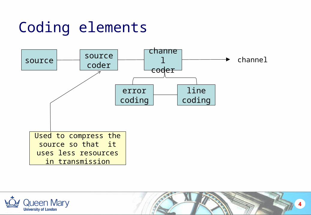
Coding elements

4

sourcesource coder

channel coder

error coding

line coding

channel

Used to compress the source so that it uses less resources in transmission

Memoryless source Probability of an event occurring does not depend on what

came before. Produces symbols (e.g. A, B, C, D) from an alphabet. Probability of a particular symbol is fixed Sum of probabilities is 1

5

Source with memory Probability of a symbol depends on previous symbol In English the probability of “u” occurring after “q” is

higher than after any other letter Lots of real sources in this category and coding like JPEG

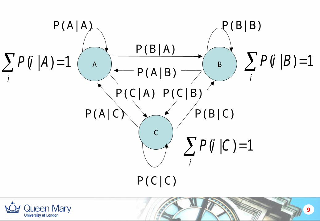
and MPEG exploits this to produce smaller file sizes Can be very complex Following example uses a Markov model to give a

memory of 1 symbol

6

Probability reminder

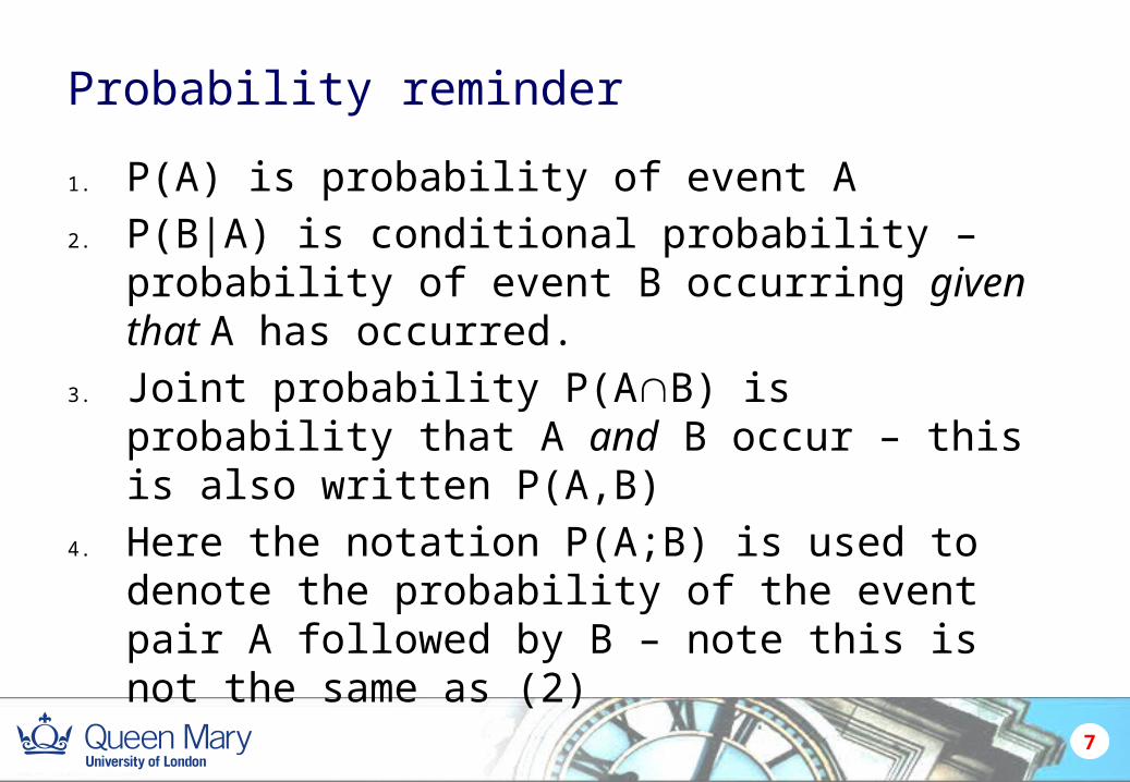
1. P(A) is probability of event A

2. P(B|A) is conditional probability – probability of event B occurring given that A has occurred.

3. Joint probability P(AB) is probability that A and B occur – this is also written P(A,B)

4. Here the notation P(A;B) is used to denote the probability of the event pair A followed by B – note this is not the same as (2)

7

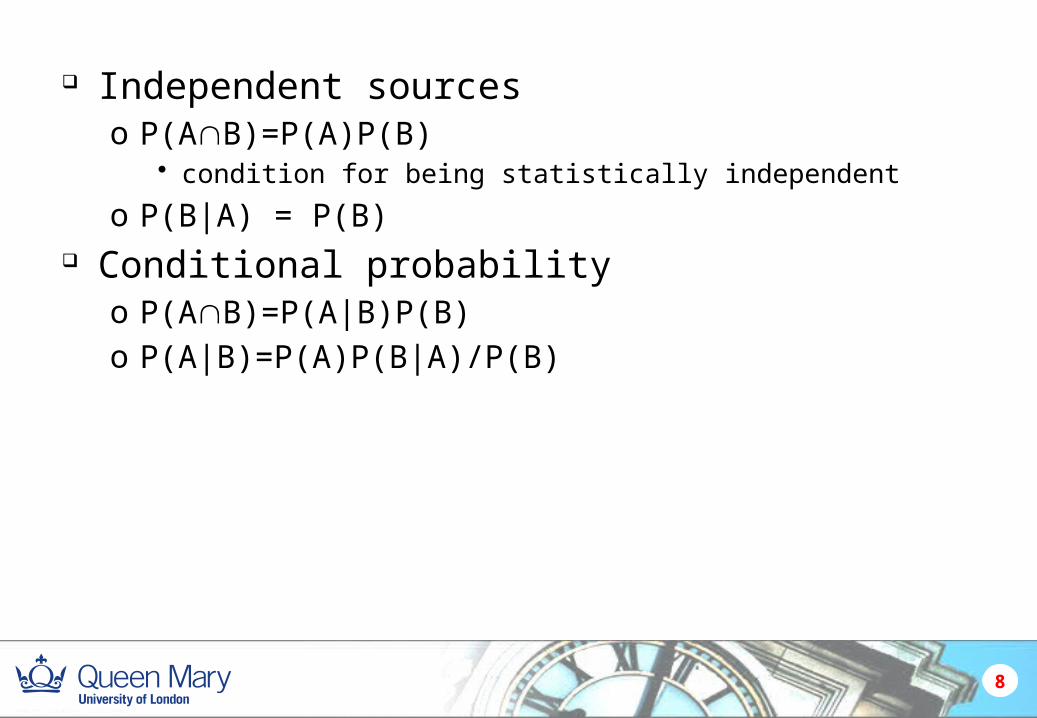
Independent sourceso P(AB)=P(A)P(B)

• condition for being statistically independent

o P(B|A) = P(B) Conditional probability

o P(AB)=P(A|B)P(B)o P(A|B)=P(A)P(B|A)/P(B)

8

9

A B

C

P(A|A)

1)|( i

AiP

P(B|C)

P(A|B)

P(A|C)

P(B|A)

P(B|B)

P(C|A) P(C|B)

P(C|C)

1)|( i

BiP

1)|( i

CiP

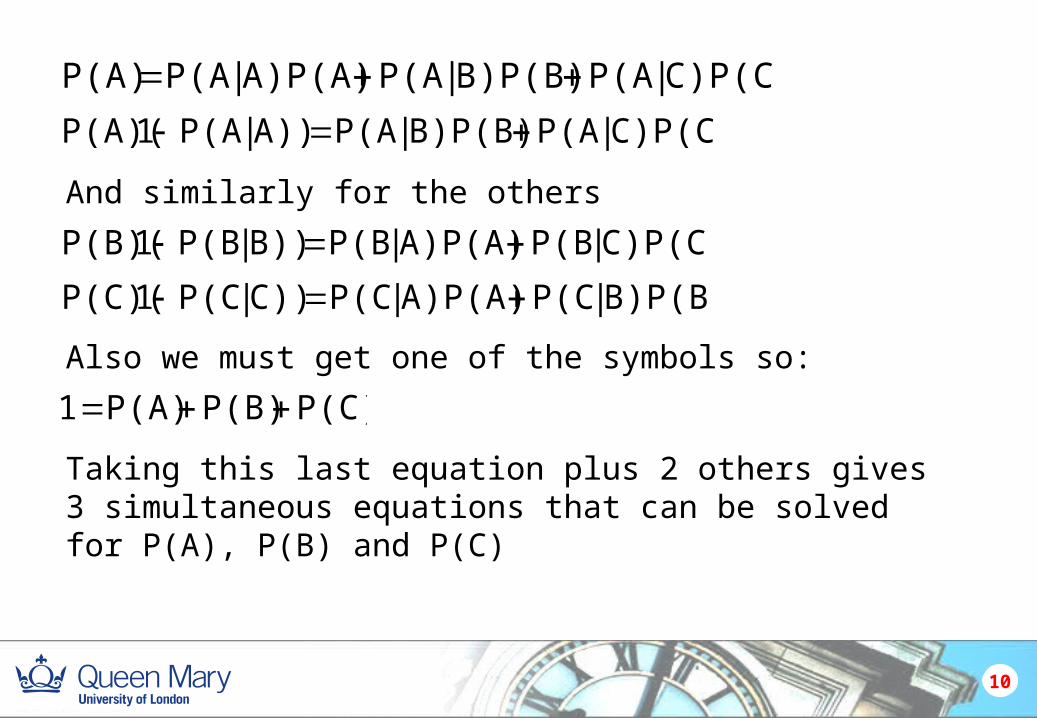
C)P(C)|P(AB)P(B)|P(AA)P(A)|P(AP(A)

10

C)P(C)|P(AB)P(B)|P(AA))|P(A1P(A)(

Taking this last equation plus 2 others gives 3 simultaneous equations that can be solved for P(A), P(B) and P(C)

P(C)P(B)P(A)1

And similarly for the others

C)P(C)|P(BA)P(A)|P(BB))|P(B1P(B)(

B)P(B)|P(CA)P(A)|P(CC))|P(C1P(C)(

Also we must get one of the symbols so:

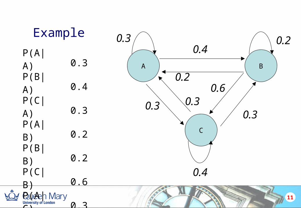
Example

11

A B

C

0.30.4

0.3

0.2

0.60.2

0.4

0.30.3

P(A|A) 0.3P(B|A) 0.4P(C|A) 0.3P(A|B) 0.2P(B|B) 0.2P(C|B) 0.6P(A|C) 0.3P(B|C) 0.3P(C|C) 0.4

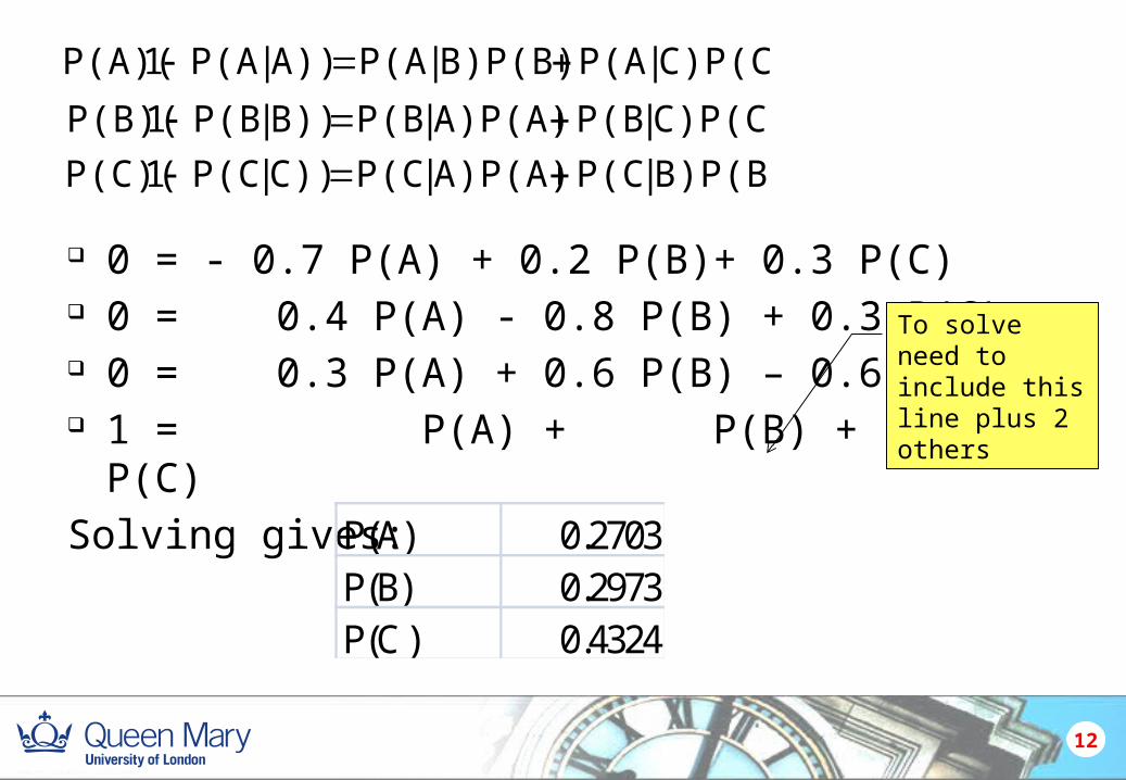
0 = - 0.7 P(A) + 0.2 P(B)+ 0.3 P(C) 0 = 0.4 P(A) - 0.8 P(B) + 0.3 P(C) 0 = 0.3 P(A) + 0.6 P(B) – 0.6 P(C) 1 = P(A) + P(B) + P(C)

Solving gives:

12

C)P(C)|P(AB)P(B)|P(AA))|P(A1P(A)(

C)P(C)|P(BA)P(A)|P(BB))|P(B1P(B)( B)P(B)|P(CA)P(A)|P(CC))|P(C1P(C)(

P(A) 0.2703P(B) 0.2973P(C ) 0.4324

To solve need to include this line plus 2 others

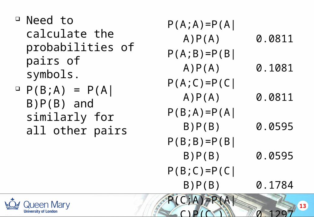
Need to calculate the probabilities of pairs of symbols.

P(B;A) = P(A|B)P(B) and similarly for all other pairs

13

P(A;A)=P(A|A)P(A) 0.0811P(A;B)=P(B|A)P(A) 0.1081P(A;C)=P(C|A)P(A) 0.0811P(B;A)=P(A|B)P(B) 0.0595P(B;B)=P(B|B)P(B) 0.0595P(B;C)=P(C|B)P(B) 0.1784P(C;A)=P(A|C)P(C ) 0.1297P(C;B)=P(B|C)P(C ) 0.1297P(C;C)=P(C|C)P(C ) 0.1730

Total 1

Information theory

What is information ?o Everything has information.o Everywhere has information.

Information in communication.o Signals: carry the information, a physical concept.o Symbols: describe the information by mathematics

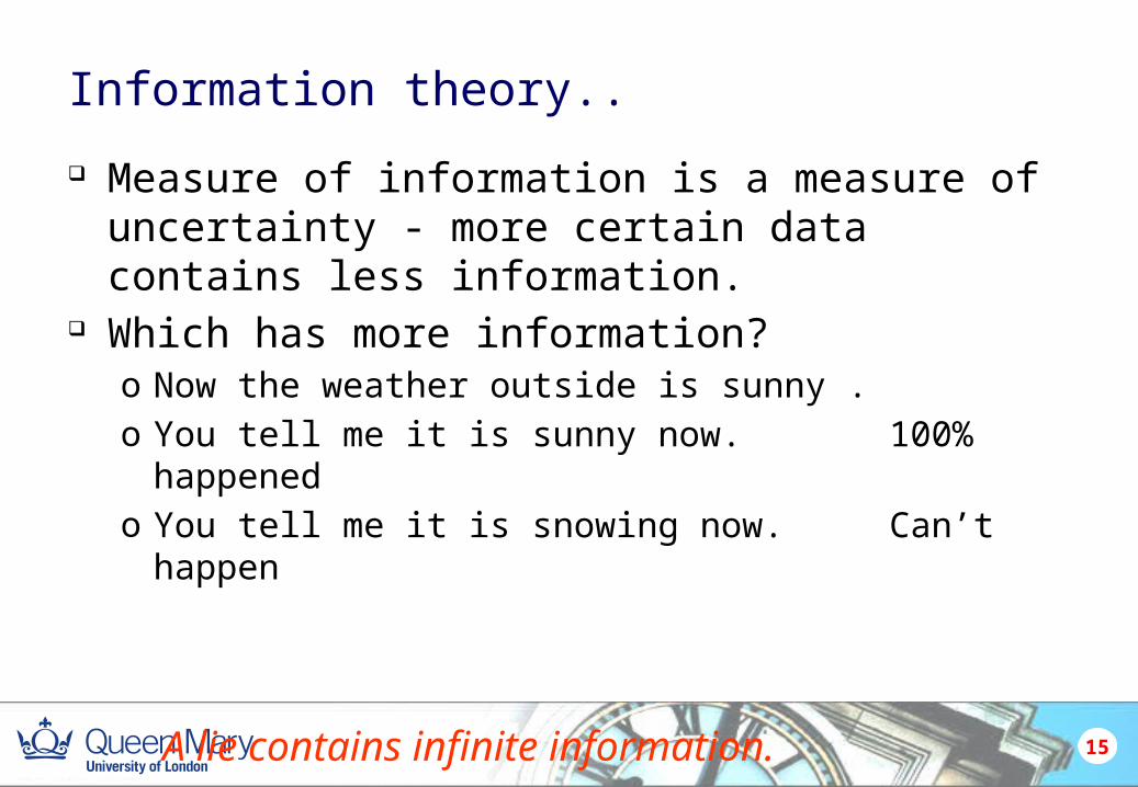
Information theory..

Measure of information is a measure of uncertainty - more certain data contains less information.

Which has more information?o Now the weather outside is sunny .o You tell me it is sunny now. 100% happened o You tell me it is snowing now. Can’t happen

A lie contains infinite information.

15

Information theory

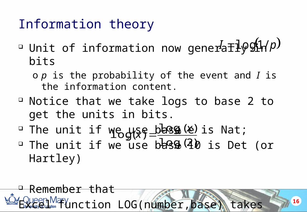
Unit of information now generally in bitso p is the probability of the event and I is the information content.

Notice that we take logs to base 2 to get the units in bits. The unit if we use base e is Nat; The unit if we use base 10 is Det (or Hartley)

Remember that

Excel function LOG(number,base) takes logs to any base.

We have 1 bit =0.693 Nat =0.301 Det

pI /1log2

16

)2(log

)(log)(log

10

102

xx

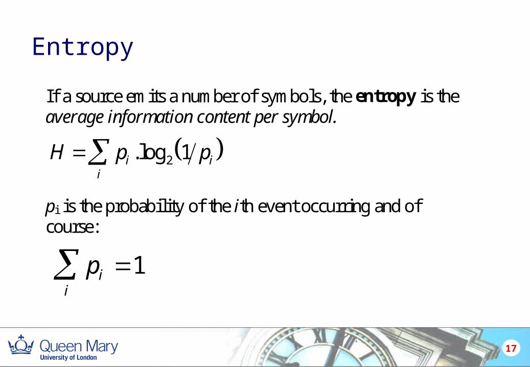
If a source emits a number of symbols, the entropy is theaverage information content per symbol.

H p pii

i .log2 1

pi is the probability of the ith event occurring and ofcourse:

pi

i 1

Entropy

17

Example

18

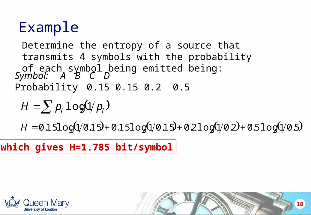
Determine the entropy of a source that transmits 4 symbols with the probability of each symbol being emitted being:

Symbol: A B C DProbability 0.15 0.15 0.2 0.5

ii ppH 1log2

5.01log5.02.01log2.015.01log15.015.01log15.0 2222 H

which gives H=1.785 bit/symbol

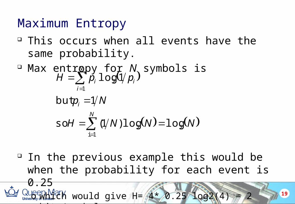
Maximum Entropy This occurs when all events have the same probability. Max entropy for N symbols is

In the previous example this would be when the probability for each event is 0.25 o which would give H= 4* 0.25 log2(4) = 2 bits/symbol

19

NNNH

Np

ppH

N

i

N

iii

221i

12

loglog)1( so

1but

1log

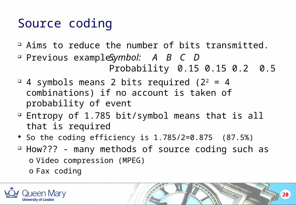
Source coding

Aims to reduce the number of bits transmitted. Previous example:

4 symbols means 2 bits required (22 = 4 combinations) if no

account is taken of probability of event Entropy of 1.785 bit/symbol means that is all that is required So the coding efficiency is 1.785/2=0.875 (87.5%) How??? - many methods of source coding such as

o Video compression (MPEG)o Fax coding

20

Symbol: A B C DProbability 0.15 0.15 0.2 0.5

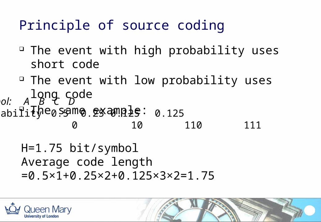
Principle of source coding

The event with high probability uses short code The event with low probability uses long code The same example:

Symbol: A B C DProbability 0.5 0.25 0.1250.125code 0 10 110 111

H=1.75 bit/symbolAverage code length =0.5×1+0.25×2+0.125×3×2=1.75

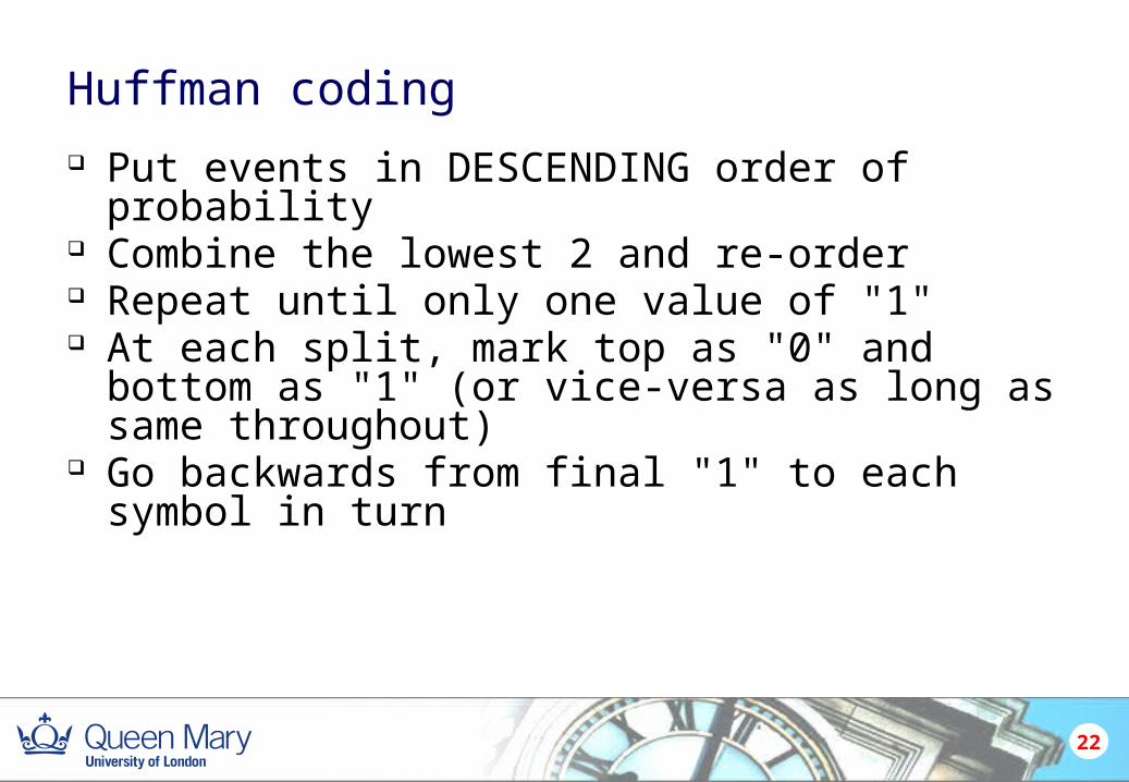
Huffman coding

Put events in DESCENDING order of probability Combine the lowest 2 and re-order Repeat until only one value of "1" At each split, mark top as "0" and bottom as "1" (or vice-

versa as long as same throughout) Go backwards from final "1" to each symbol in turn

22

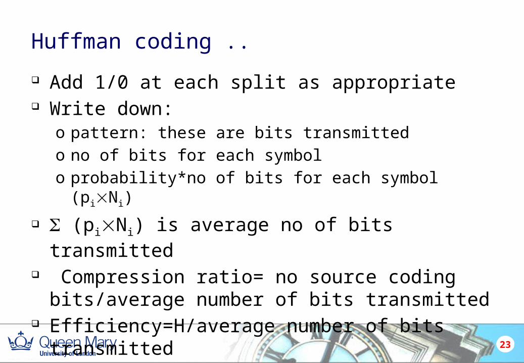
Add 1/0 at each split as appropriate Write down:

o pattern: these are bits transmittedo no of bits for each symbolo probability*no of bits for each symbol (piNi)

(piNi) is average no of bits transmitted Compression ratio= no source coding bits/average

number of bits transmitted Efficiency=H/average number of bits transmitted

Huffman coding ..

23

D 0.5 C 0.2 B 0.15 A 0.15

24

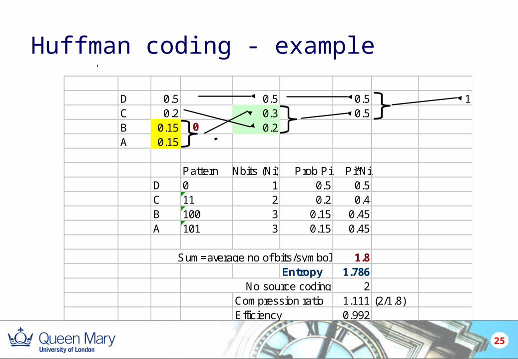
Huffman coding - example

25

D 0.5 0.5 0.5 1C 0.2 0.3 0.5B 0.15 0.2A 0.15

Pattern Nbits (Ni) Prob Pi Pi*NiD 0 1 0.5 0.5C 11 2 0.2 0.4B 100 3 0.15 0.45A 101 3 0.15 0.45

1.8Entropy 1.786

2Compression ratio 1.111 (2/1.8)Efficiency 0.992

Sum=average no of bits/symbol

No source coding

01

01

01

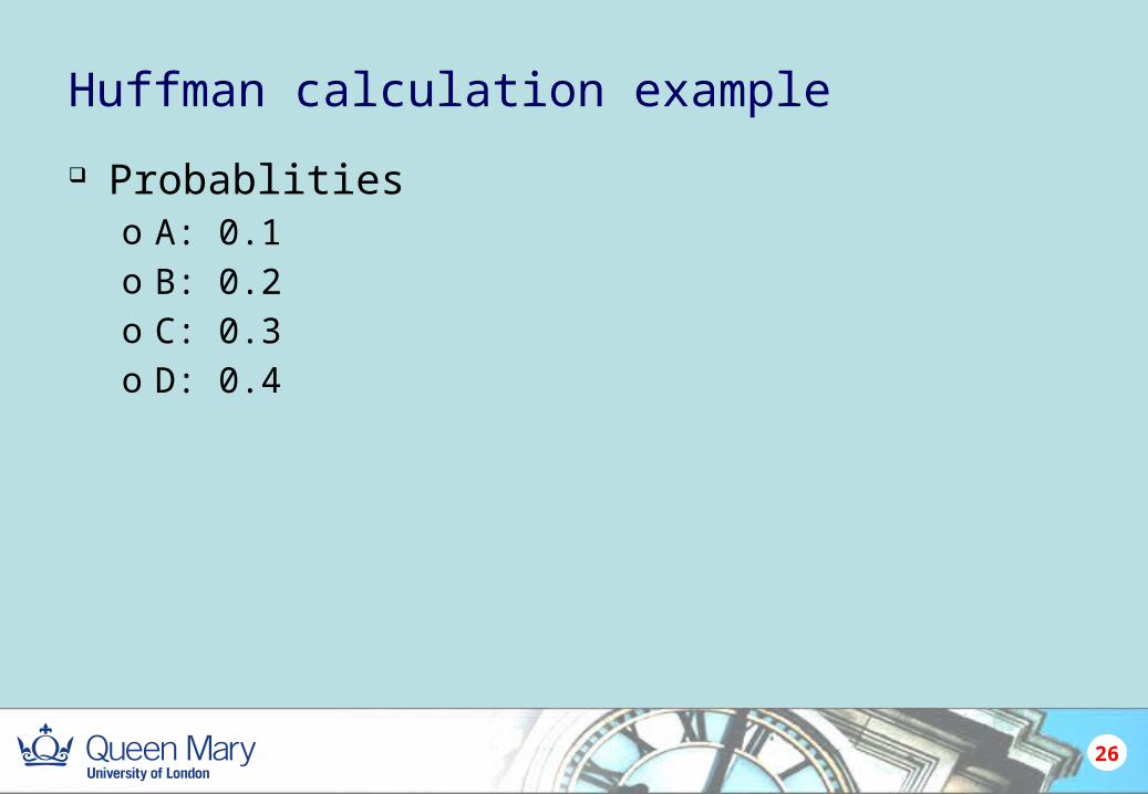
Huffman calculation example

Probablitieso A: 0.1o B: 0.2o C: 0.3o D: 0.4

26

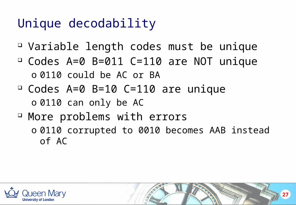
Unique decodability

Variable length codes must be unique Codes A=0 B=011 C=110 are NOT unique

o 0110 could be AC or BA Codes A=0 B=10 C=110 are unique

o 0110 can only be AC More problems with errors

o 0110 corrupted to 0010 becomes AAB instead of AC

27

Run-length codes

Code the number of times something occurs, not the individual events

e.g. row of pixels across a page (fax) e.g. row of pixels across a page (fax) e.g. row of pixels across a page (fax) Fax transmission (see resources section) Codes each sequence of black or white into a partitioned

code word

Middle of line of text above

28

1728 pixels in each row Each pixel maybe white or black So there are 2×1728 codes in total, very complex,

need large storage Revised Huffman coding

o Terminating codes R (0<L≤63) omakeup codes K, multiples of 64o L =64K+R, (64<L<1728)

Run-length codes

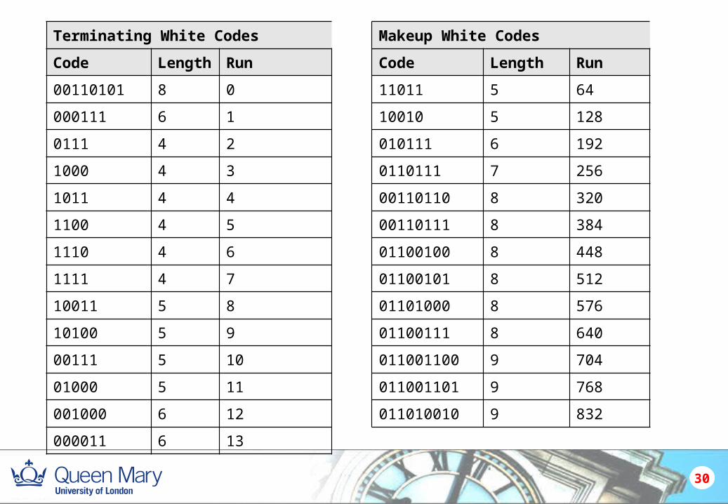
Terminating White Codes

Code Length Run

00110101 8 0

000111 6 1

0111 4 2

1000 4 3

1011 4 4

1100 4 5

1110 4 6

1111 4 7

10011 5 8

10100 5 9

00111 5 10

01000 5 11

001000 6 12

000011 6 13

Makeup White Codes

Code Length Run

11011 5 64

10010 5 128

010111 6 192

0110111 7 256

00110110 8 320

00110111 8 384

01100100 8 448

01100101 8 512

01101000 8 576

01100111 8 640

011001100 9 704

011001101 9 768

011010010 9 832

30

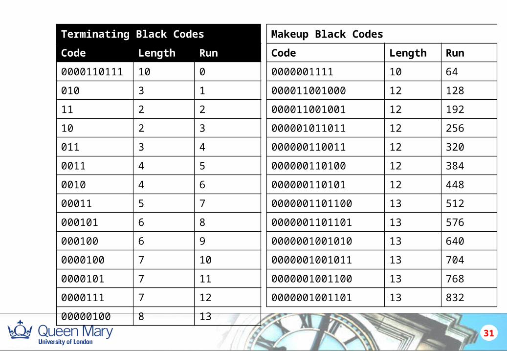
Terminating Black Codes

Code Length Run

0000110111 10 0

010 3 1

11 2 2

10 2 3

011 3 4

0011 4 5

0010 4 6

00011 5 7

000101 6 8

000100 6 9

0000100 7 10

0000101 7 11

0000111 7 12

00000100 8 13

Makeup Black Codes

Code Length Run

0000001111 10 64

000011001000 12 128

000011001001 12 192

000001011011 12 256

000000110011 12 320

000000110100 12 384

000000110101 12 448

0000001101100 13 512

0000001101101 13 576

0000001001010 13 640

0000001001011 13 704

0000001001100 13 768

0000001001101 13 832

31

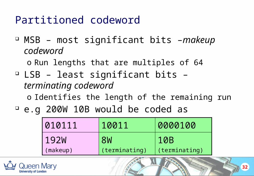
Partitioned codeword

MSB – most significant bits –makeup codewordo Run lengths that are multiples of 64

LSB – least significant bits – terminating codewordo Identifies the length of the remaining run

e.g 200W 10B would be coded as

010111 10011 0000100

192W (makeup)

8W (terminating)

10B (terminating)

32

LPZ code (ZIP)

Does not need to have probabilities in advance Look up

33

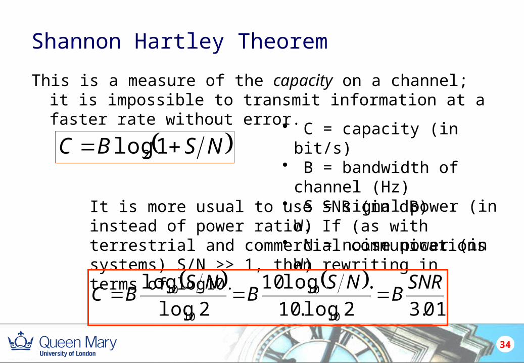
Shannon Hartley Theorem

This is a measure of the capacity on a channel; it is impossible to transmit information at a faster rate without error.

NSBC 1log2

• C = capacity (in bit/s)• B = bandwidth of channel (Hz)• S = signal power (in W)• N = noise power (in W)

It is more usual to use SNR (in dB) instead of power ratio. If (as with terrestrial and commercial communications systems) S/N >> 1, then rewriting in terms of log10.

01.32log.10

.log10

2log

log

10

10

10

10 SNRB

NSB

NSBC

34

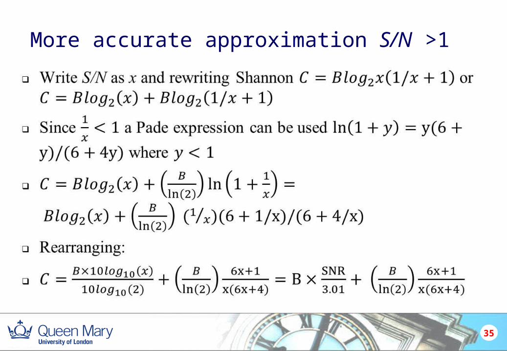
More accurate approximation S/N >1

35

S/N<1

36

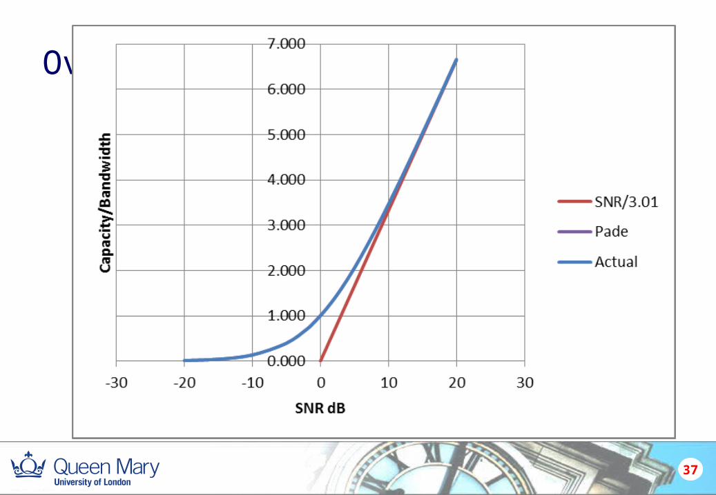
Overall effect

37

AWGN

Strictly Shannon Hartley is for AWGN (Additive White Gaussian Noise)

Linear addition of white noise with a constant spectral density (expressed as watts per hertz of bandwidth) and a Gaussian distribution of amplitude.

Does not account for fading, frequency selectivity, interference, nonlinearity or dispersion.

38

Shannon and AWGN

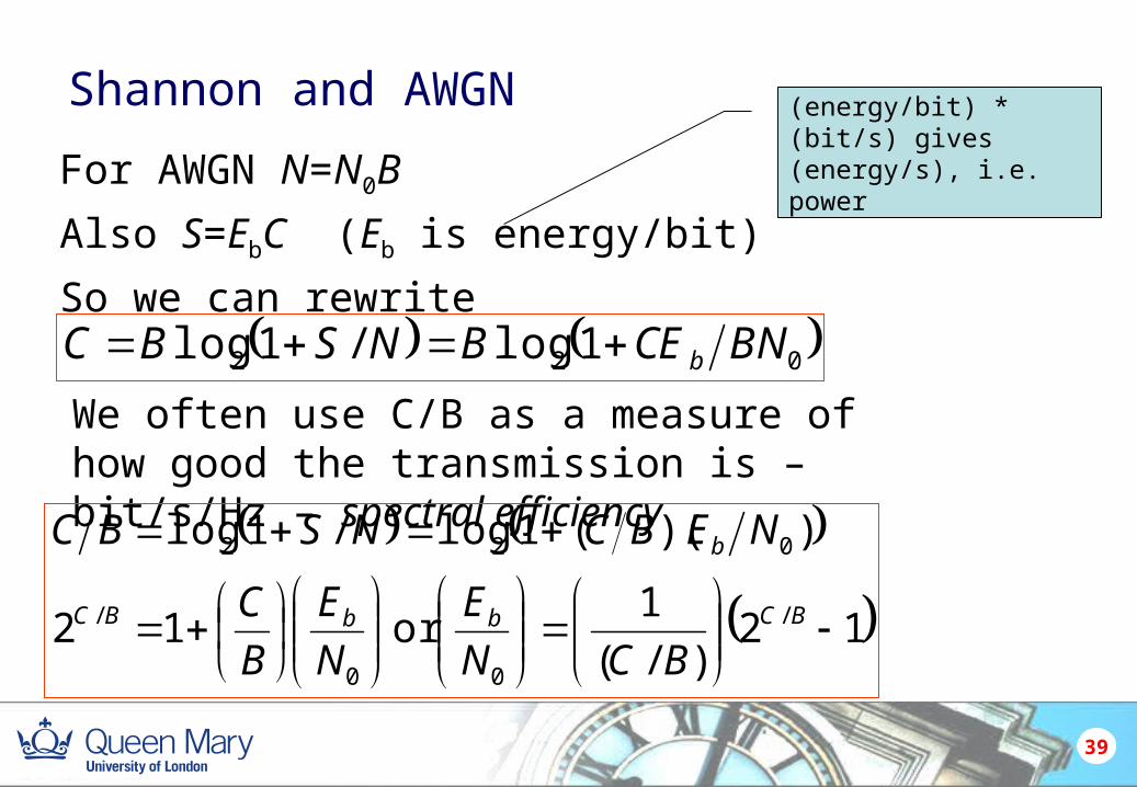
For AWGN N=N0B

Also S=EbC (Eb is energy/bit)

So we can rewrite

39

(energy/bit) * (bit/s) gives (energy/s), i.e. power

022 1log/1log BNCEBNSBC b

12)/(

1or 12

))((1log/1log

/

00

/

022

BCbbBC

b

BCN

E

N

E

B

C

NEBCNSBC

We often use C/B as a measure of how good the transmission is – bit/s/Hz – spectral efficiency

Usable region

40

0.001

0.01

0.1

1

10

-5 0 5 10 15 20 25 30 35 40

(Eb/No) in dB

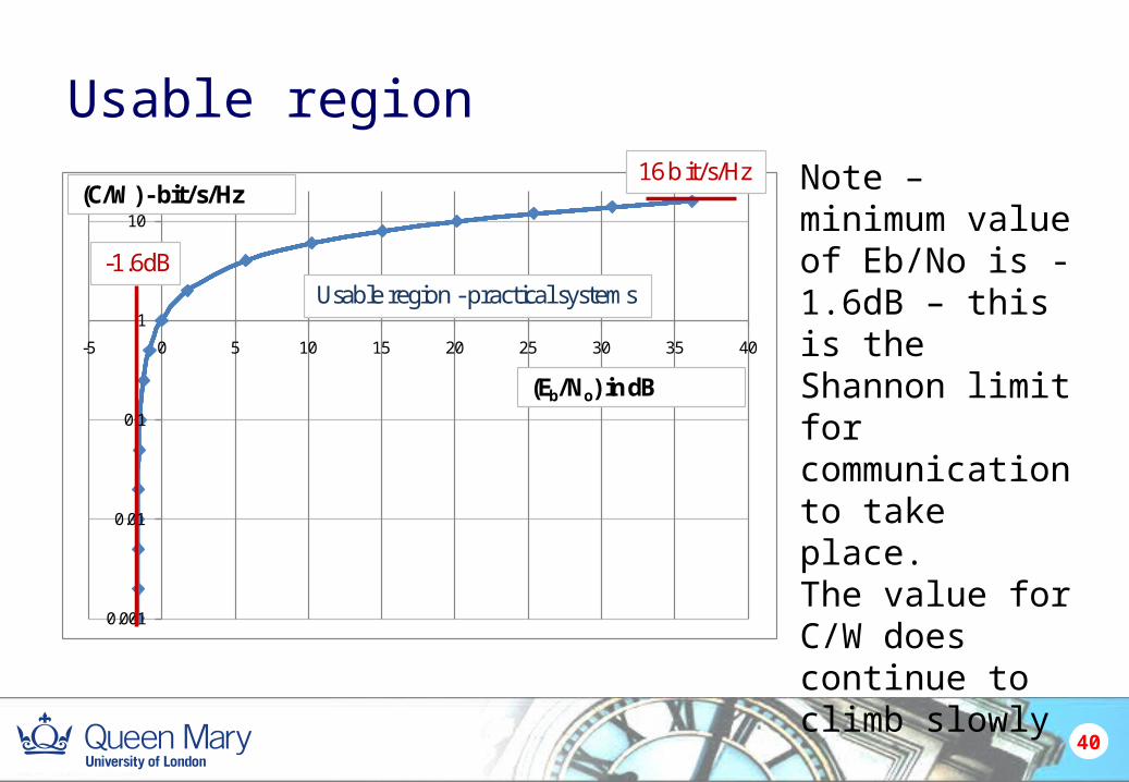
(C/W) - bit/s/Hz16 b it/s/Hz

-1.6dBUsable region - practical systems

Note – minimum value of Eb/No is -1.6dB – this is the Shannon limit for communication to take place.The value for C/W does continue to climb slowly

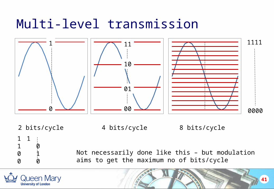
Multi-level transmission

41

2 bits/cycle 4 bits/cycle

1

0

11

10

01

00

8 bits/cycle

1111

0000

1 11 00 10 0

Not necessarily done like this – but modulationaims to get the maximum no of bits/cycle

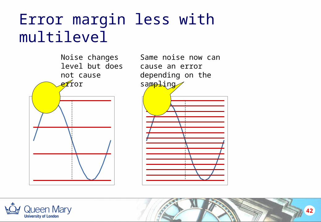
Error margin less with multilevel

42

Noise changes level but does not cause error

Same noise now can cause an error depending on the sampling

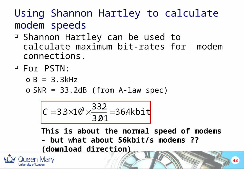
Using Shannon Hartley to calculate modem speeds

Shannon Hartley can be used to calculate maximum bit-rates for modem connections.

For PSTN:o B = 3.3kHzo SNR = 33.2dB (from A-law spec)

kbit/s4.3601.3

2.33103.3 3 C

This is about the normal speed of modems - but what about 56kbit/s modems ?? (download direction)

43

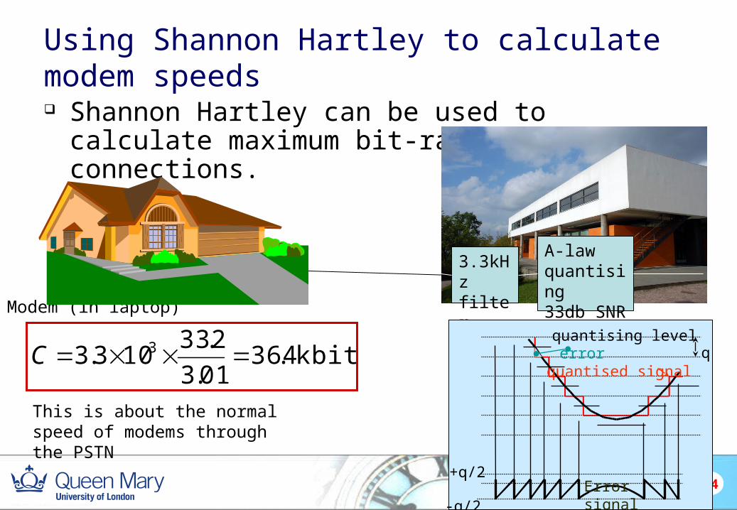
Using Shannon Hartley to calculate modem speeds

Shannon Hartley can be used to calculate maximum bit-rates for modem connections.

44

Modem (in laptop)

3.3kHzfilter

A-lawquantising33db SNR

kbit/s4.3601.3

2.33103.3 3 C

This is about the normal speed of modems through the PSTN

-q/2

quantising levelerror q

Errorsignal

+q/2

quantised signal

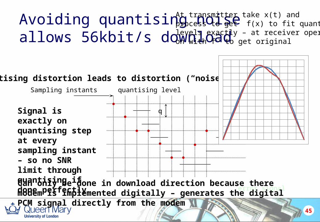
Avoiding quantising noiseallows 56kbit/s download

45

quantising levelSampling instants

q

error signal

Quantising distortion leads to distortion (“noise”)

Signal is exactly on quantising step at every sampling instant – so no SNR limit through quantising if done perfectly

Can only be done in download direction because there modem is implemented digitally – generates the digital PCM signal directly from the modem

At transmitter take x(t) and process to get f(x) to fit quantisinglevels exactly – at receiver operateon with f-1 to get original

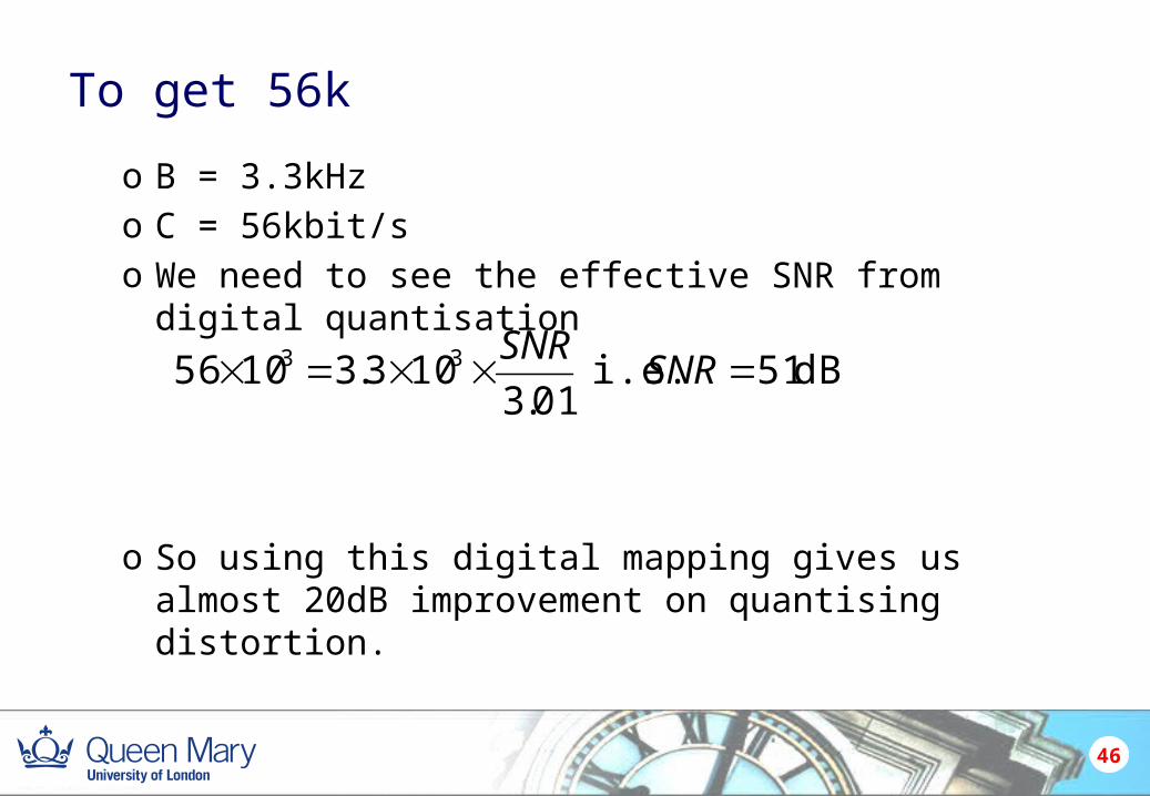
To get 56k

o B = 3.3kHzo C = 56kbit/so We need to see the effective SNR from digital quantisation

o So using this digital mapping gives us almost 20dB improvement on quantising distortion.

dB51 i.e. 01.3

103.31056 33 SNRSNR

46

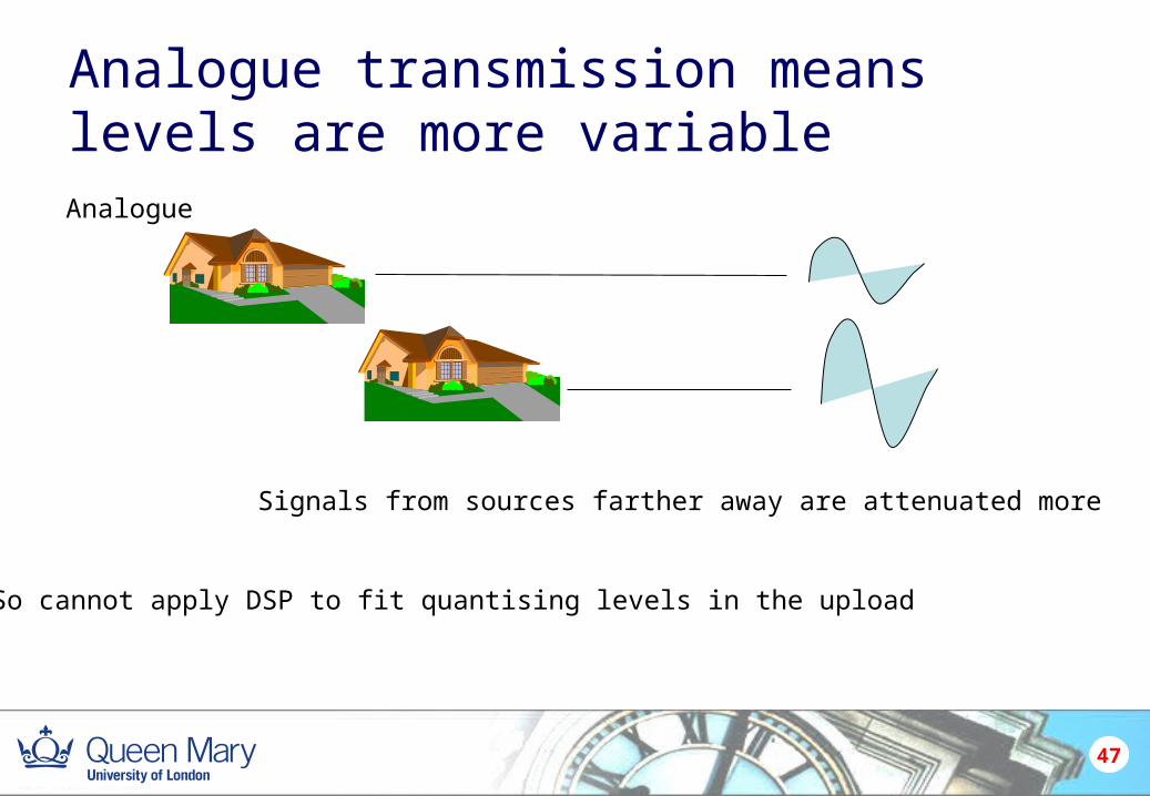
Analogue transmission means levels are more variable

47

Analogue

Signals from sources farther away are attenuated more

So cannot apply DSP to fit quantising levels in the upload

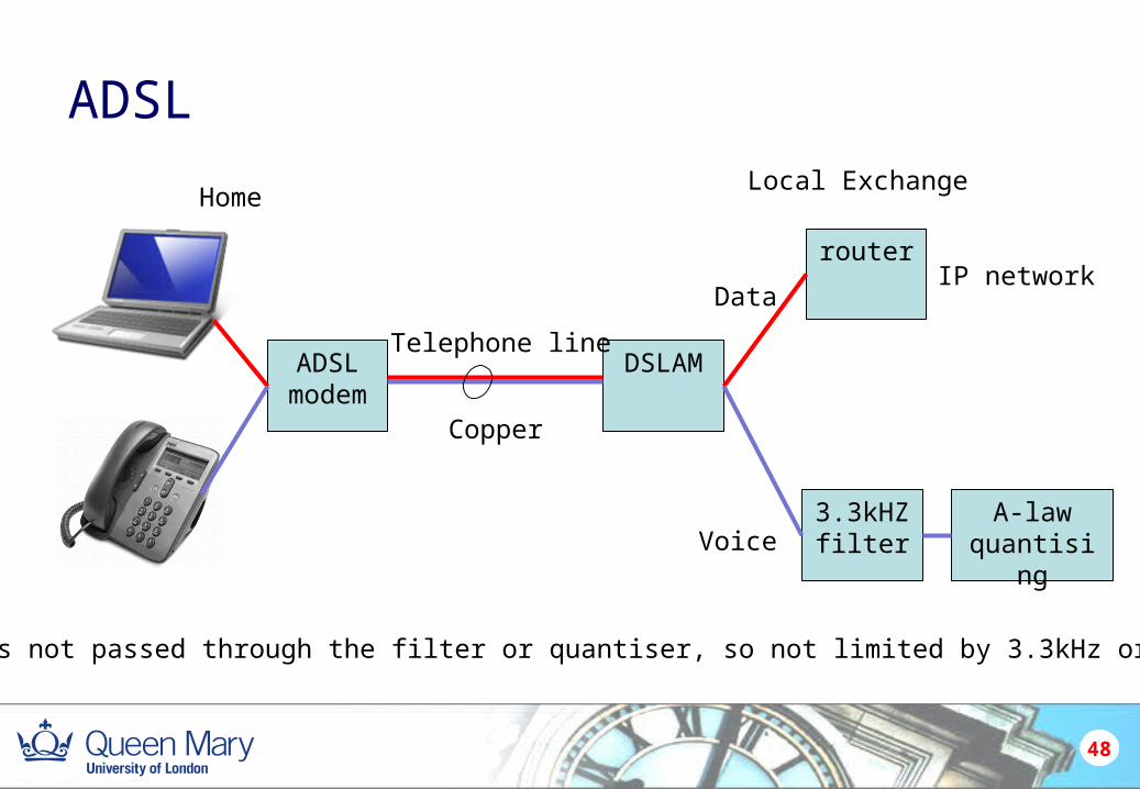
ADSL

48

ADSL modem

DSLAM

router

3.3kHZfilter

A-lawquantising

HomeLocal Exchange

Telephone line

Data

Voice

IP network

Data is not passed through the filter or quantiser, so not limited by 3.3kHz or 33dB SNR

Copper

Binary symmetric channel

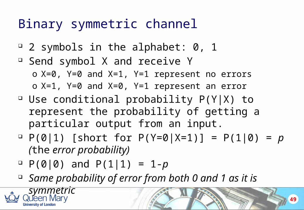
2 symbols in the alphabet: 0, 1 Send symbol X and receive Y

o X=0, Y=0 and X=1, Y=1 represent no errorso X=1, Y=0 and X=0, Y=1 represent an error

Use conditional probability P(Y|X) to represent the probability of getting a particular output from an input.

P(0|1) [short for P(Y=0|X=1)] = P(1|0) = p (the error probability)

P(0|0) and P(1|1) = 1-p Same probability of error from both 0 and 1 as it is symmetric

49

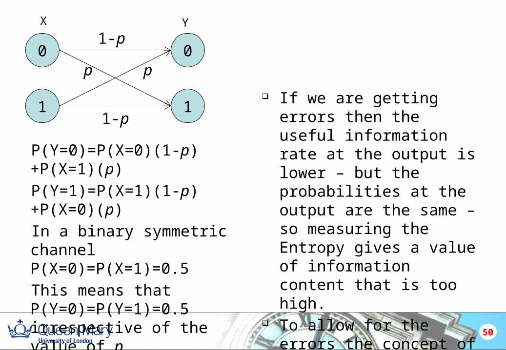
P(Y=0)=P(X=0)(1-p)+P(X=1)(p)

P(Y=1)=P(X=1)(1-p)+P(X=0)(p)

In a binary symmetric channel P(X=0)=P(X=1)=0.5

This means that P(Y=0)=P(Y=1)=0.5 irrespective of the value of p

If we are getting errors then the useful information rate at the output is lower – but the probabilities at the output are the same – so measuring the Entropy gives a value of information content that is too high.

To allow for the errors the concept of Equivocation is used.

50

0

1 1

0

X Y

p p

1-p

1-p

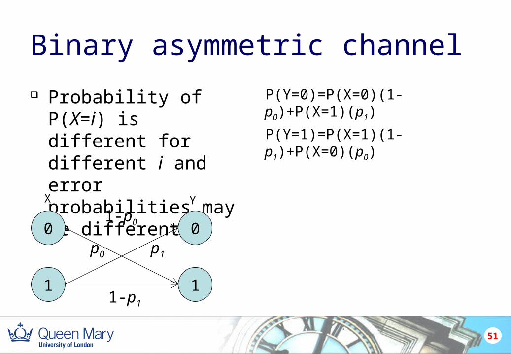
Binary asymmetric channel

Probability of P(X=i) is different for different i and error probabilities may be different.

P(Y=0)=P(X=0)(1-p0)+P(X=1)(p1)

P(Y=1)=P(X=1)(1-p1)+P(X=0)(p0)

51

0

1 1

0

X Y

p0 p1

1-p0

1-p1

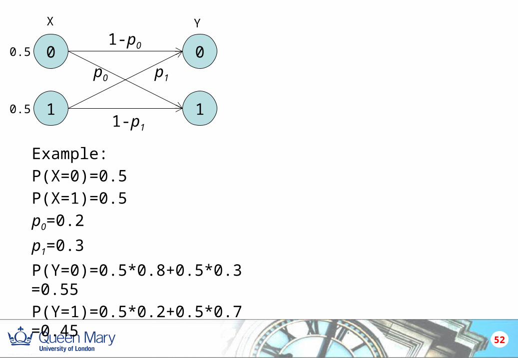
Example:

P(X=0)=0.5

P(X=1)=0.5

p0=0.2

p1=0.3

P(Y=0)=0.5*0.8+0.5*0.3=0.55

P(Y=1)=0.5*0.2+0.5*0.7=0.45

52

0

1 1

0

X Y

p0 p1

1-p0

1-p1

0.5

0.5

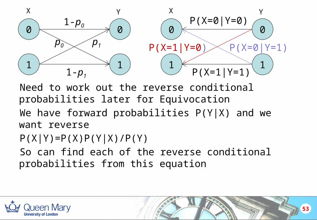
Need to work out the reverse conditional probabilities later for Equivocation

We have forward probabilities P(Y|X) and we want reverse

P(X|Y)=P(X)P(Y|X)/P(Y)

So can find each of the reverse conditional probabilities from this equation

53

0

1 1

0

X Y

p0 p1

1-p0

1-p1

0

1 1

0

X YP(X=0|Y=0)

P(X=0|Y=1)

P(X=1|Y=1)

P(X=1|Y=0)

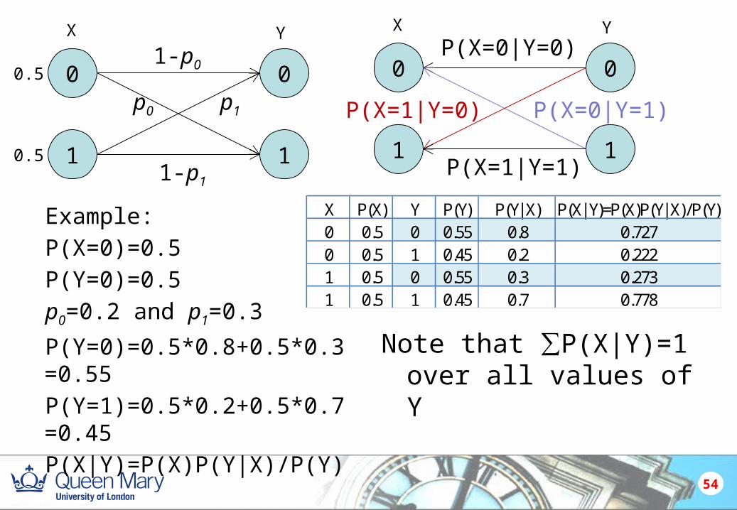
Example:

P(X=0)=0.5

P(Y=0)=0.5

p0=0.2 and p1=0.3

P(Y=0)=0.5*0.8+0.5*0.3=0.55

P(Y=1)=0.5*0.2+0.5*0.7=0.45

P(X|Y)=P(X)P(Y|X)/P(Y)

Note that ∑P(X|Y)=1 over all values of Y

54

0

1 1

0

X Y

p0 p1

1-p0

1-p1

0.5

0.5

0

1 1

0

X YP(X=0|Y=0)

P(X=0|Y=1)

P(X=1|Y=1)

P(X=1|Y=0)

X P(X) Y P(Y) P(Y|X) P(X|Y)=P(X)P(Y|X)/P(Y)0 0.5 0 0.55 0.8 0.7270 0.5 1 0.45 0.2 0.2221 0.5 0 0.55 0.3 0.2731 0.5 1 0.45 0.7 0.778

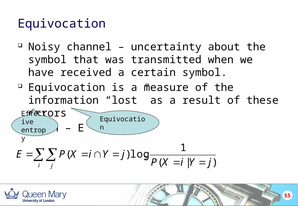
Equivocation

Noisy channel – uncertainty about the symbol that was transmitted when we have received a certain symbol.

Equivocation is a measure of the information “lost” as a result of these errors

Heff=H – E

55

Effective entropy

Equivocation

)|(

1log)( 2 jYiXP

jYiXPEi j

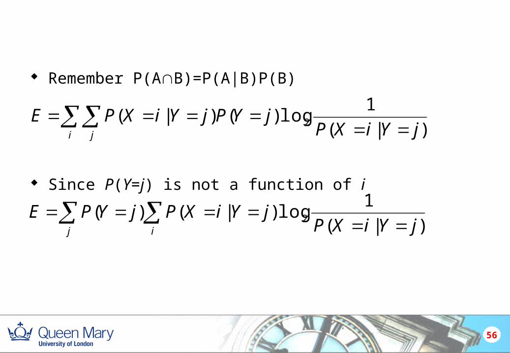
Remember P(AB)=P(A|B)P(B)

Since P(Y=j) is not a function of i

56

)|(

1log)()|( 2 jYiXP

jYPjYiXPEi j

)|(

1log)|()( 2 jYiXP

jYiXPjYPEj i

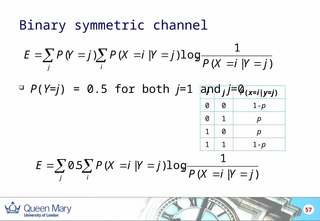
Binary symmetric channel

P(Y=j) = 0.5 for both j=1 and j=0

57

)|(

1log)|()( 2 jYiXP

jYiXPjYPEj i

i j P(x=i|y=j)

0 0 1-p

0 1 p

1 0 p

1 1 1-p

)|(

1log)|(5.0 2 jYiXP

jYiXPEj i

58

)|(

1log)|(5.0 2 jYiXP

jYiXPEj i

)1|1(/1log)1|1(

)1|0(/1log)1|0(

)0|1(/1log)0|1(

)0|0(/1log)0|0(

5.0

2

2

2

2

YXPYXP

YXPYXP

YXPYXP

YXPYXP

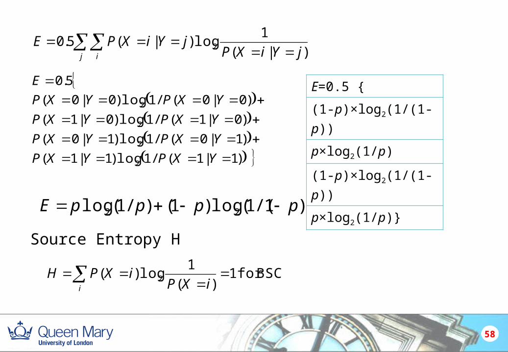
E E=0.5 {

(1-p)×log2(1/(1-p))

p×log2(1/p)

(1-p)×log2(1/(1-p))

p×log2(1/p)}

))1/(1(log)1()/1(log 22 ppppE

Source Entropy H

BSCfor 1)(

1log)( 2

iXP

iXPHi

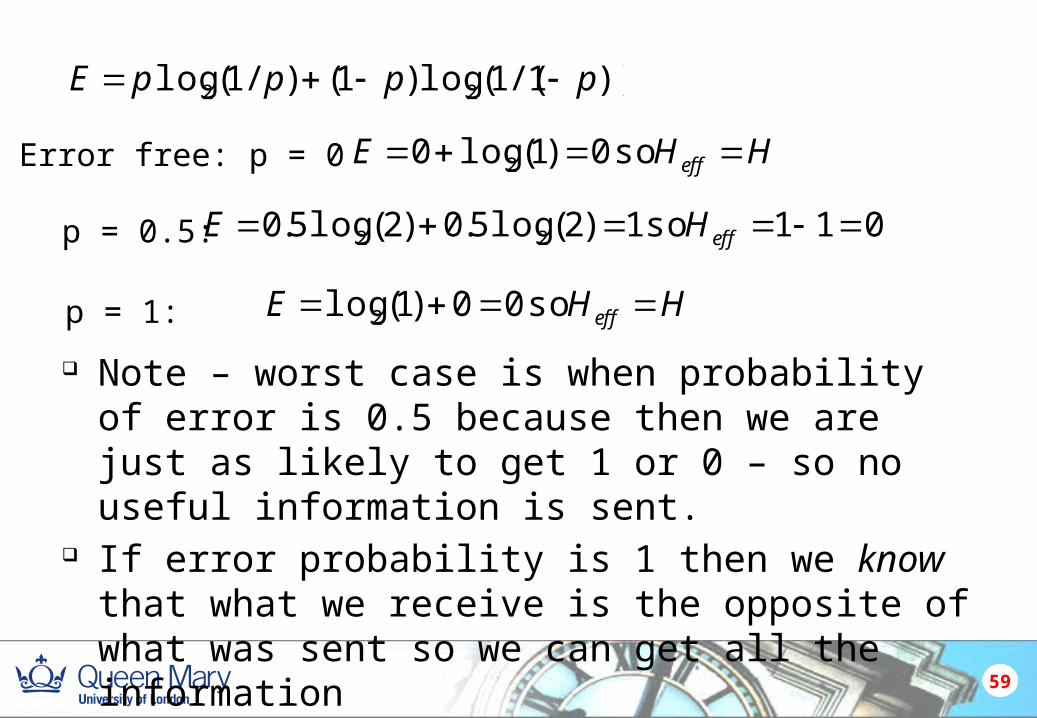
Note – worst case is when probability of error is 0.5 because then we are just as likely to get 1 or 0 – so no useful information is sent.

If error probability is 1 then we know that what we receive is the opposite of what was sent so we can get all the information

59

))1/(1(log)1()/1(log 22 ppppE

Error free: p = 0 HHE eff so 0)1(log0 2

p = 0.5: 011 so 1)2(log5.0)2(log5.0 22 effHE

p = 1: HHE eff so 00)1(log 2

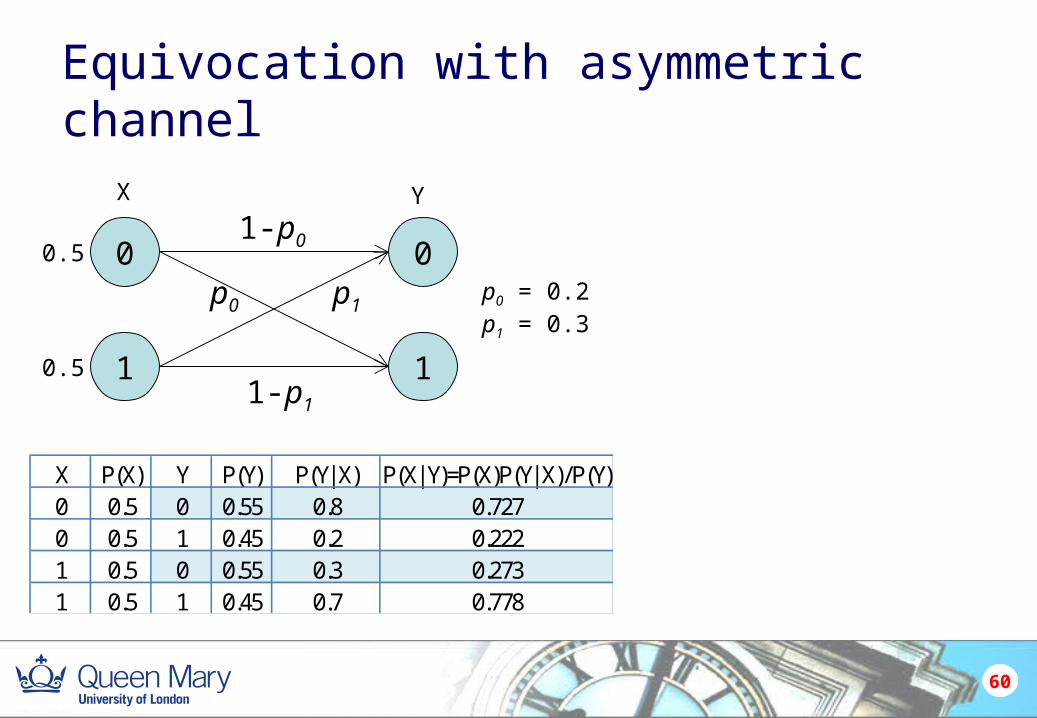
Equivocation with asymmetric channel

60

0

1 1

0

X Y

p0 p1

1-p0

1-p1

0.5

0.5

p0 = 0.2p1 = 0.3

X P(X) Y P(Y) P(Y|X) P(X|Y)=P(X)P(Y|X)/P(Y)0 0.5 0 0.55 0.8 0.7270 0.5 1 0.45 0.2 0.2221 0.5 0 0.55 0.3 0.2731 0.5 1 0.45 0.7 0.778

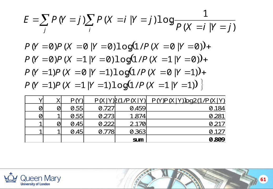
61

)1|1(/1log)1|1()1(

)1|0(/1log)1|0()1(

)0|1(/1log)0|1()0(

)0|0(/1log)0|0()0(

2

2

2

2

YXPYXPYP

YXPYXPYP

YXPYXPYP

YXPYXPYP

)|(

1log)|()( 2 jYiXP

jYiXPjYPEj i

Y X P(Y) P(X|Y)log2(1/P(X|Y) P(Y)P(X|Y)log2(1/P(X|Y)0 0 0.55 0.727 0.459 0.1840 1 0.55 0.273 1.874 0.2811 0 0.45 0.222 2.170 0.2171 1 0.45 0.778 0.363 0.127

sum 0.809

ERRORS AND IMPAIRMENTS

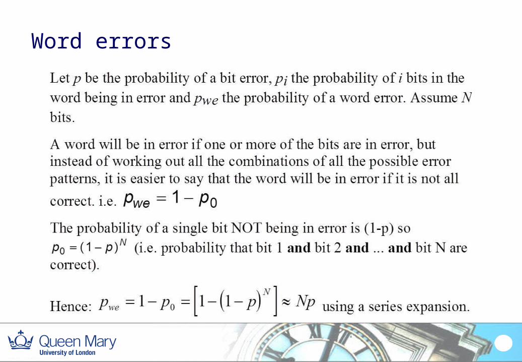
Word errors

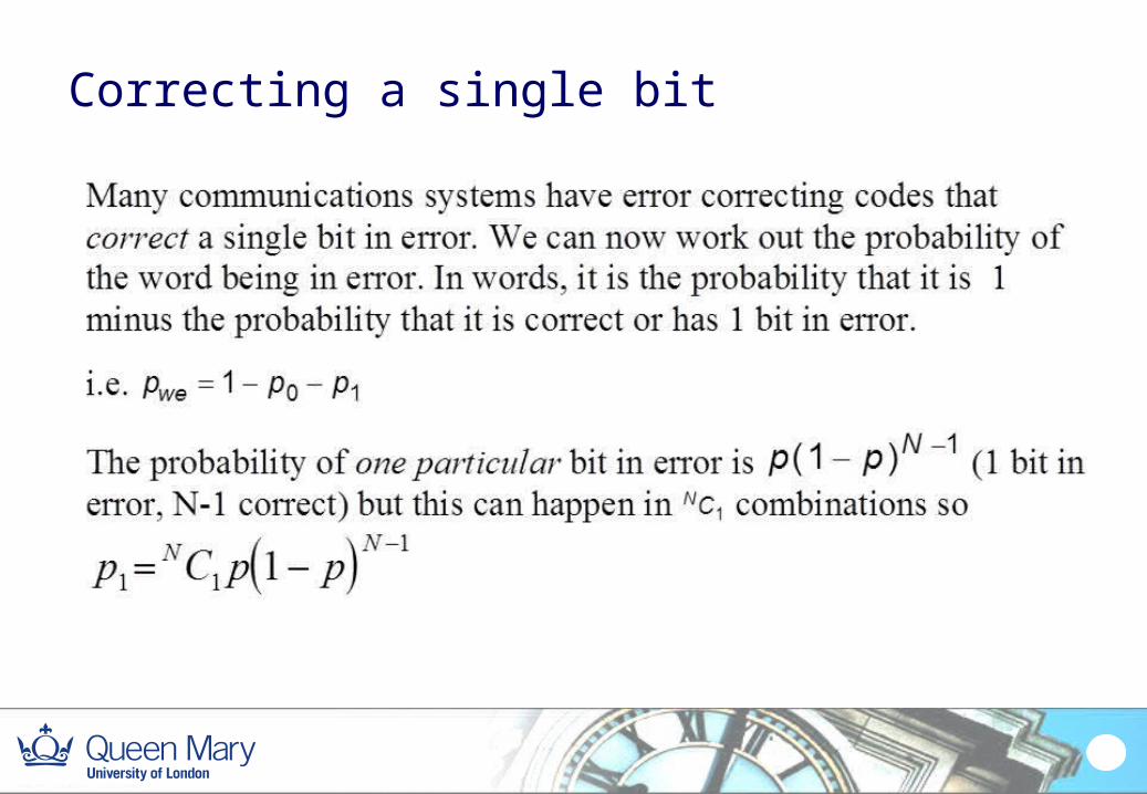
Correcting a single bit

….

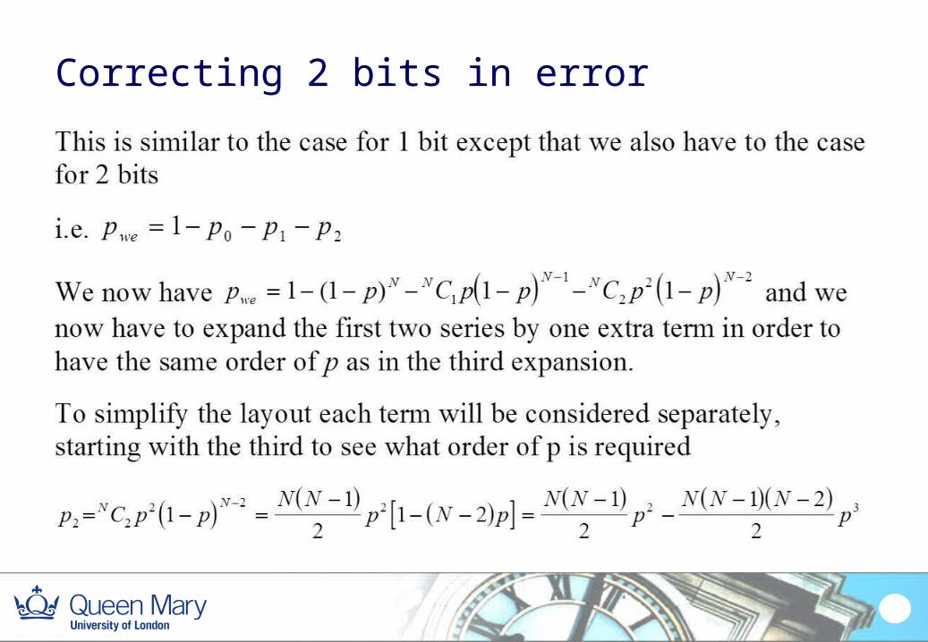
Correcting 2 bits in error

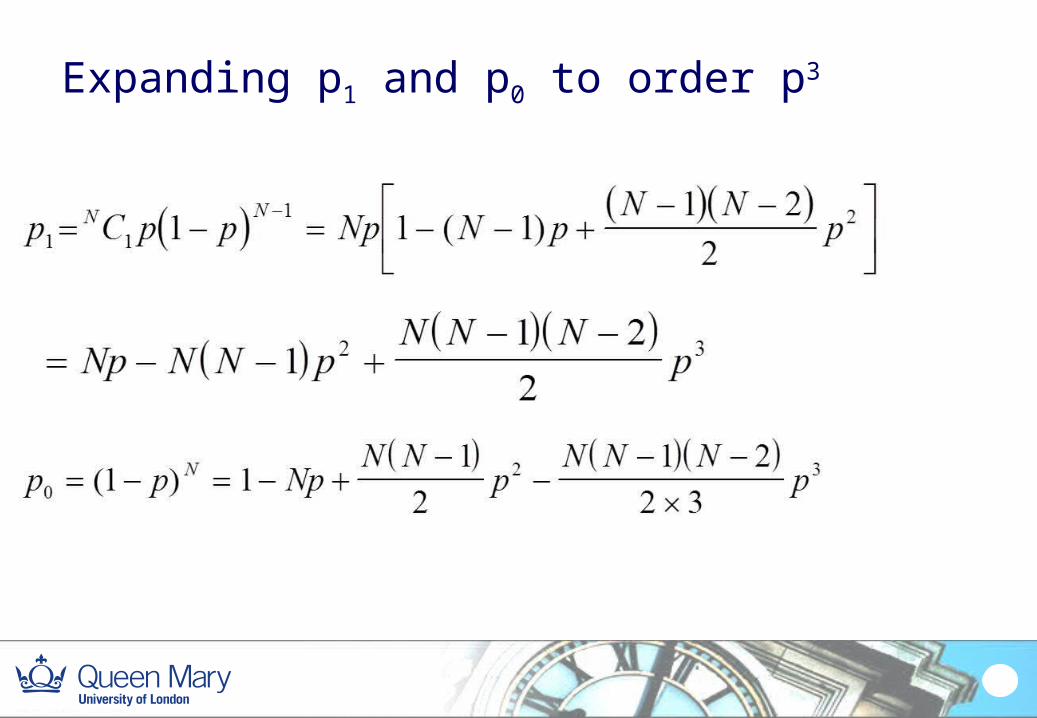
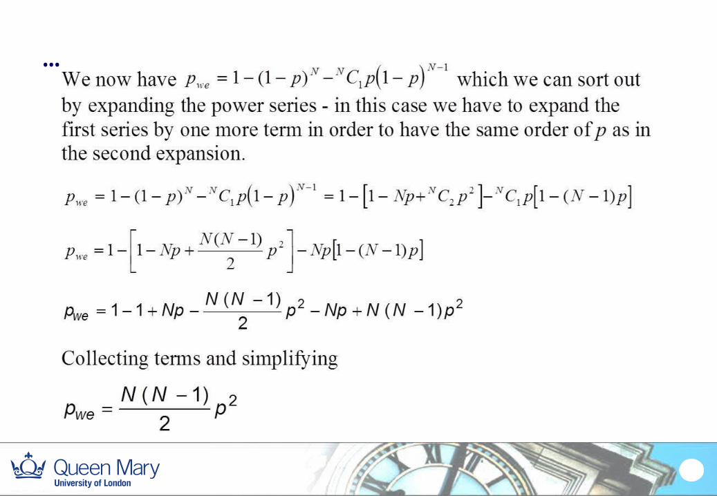
Expanding p1 and p0 to order p3

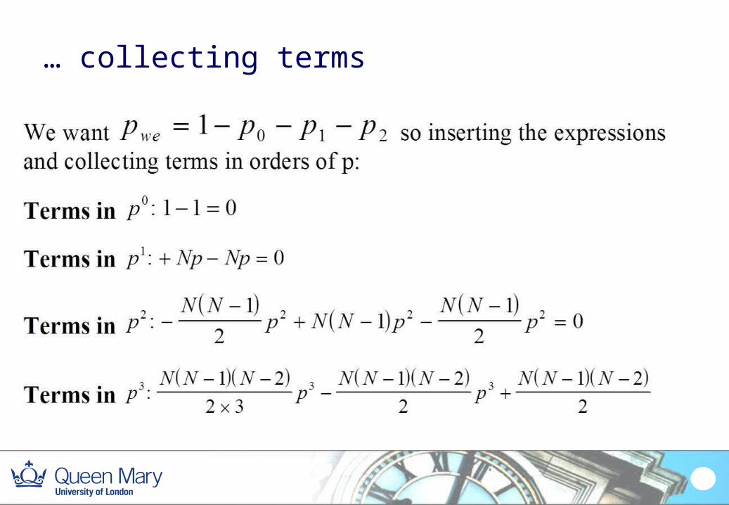
… collecting terms

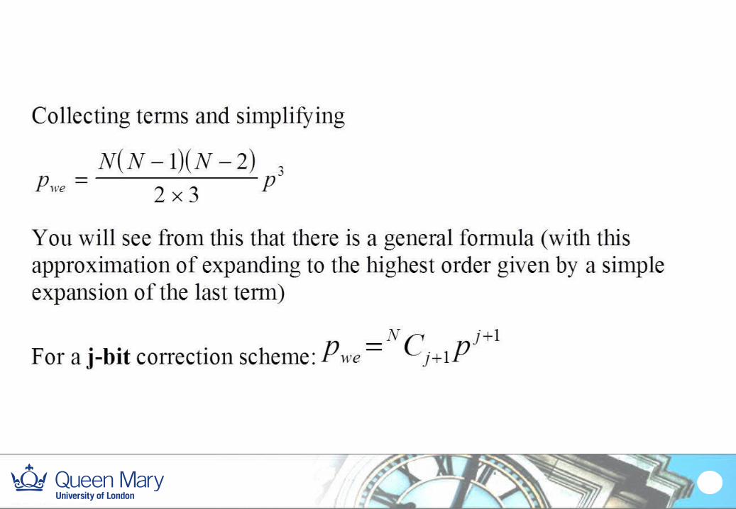
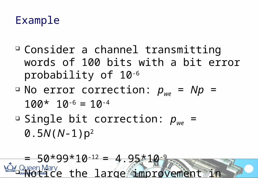
Example

Consider a channel transmitting words of 100 bits with a bit error probability of 10-6

No error correction: pwe = Np = 100* 10-6 = 10-4

Single bit correction: pwe = 0.5N(N-1)p2

= 50*99*10-12 = 4.95*10-9

Notice the large improvement in error probability.

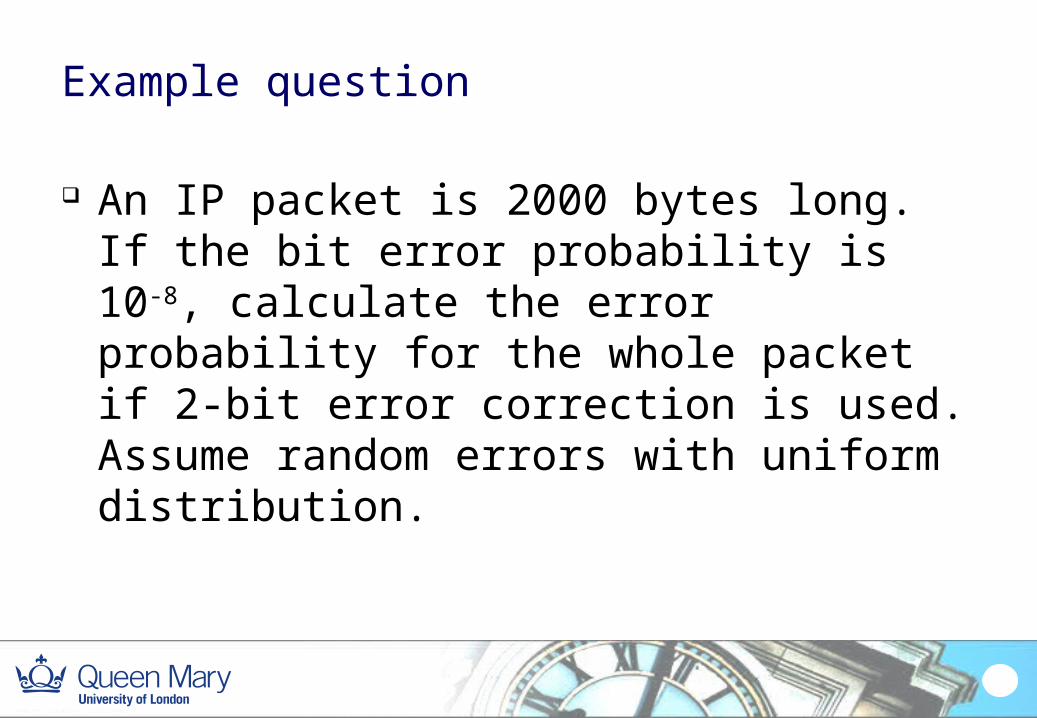
Example question

An IP packet is 2000 bytes long. If the bit error probability is 10-8, calculate the error probability for the whole packet if 2-bit error correction is used. Assume random errors with uniform distribution.

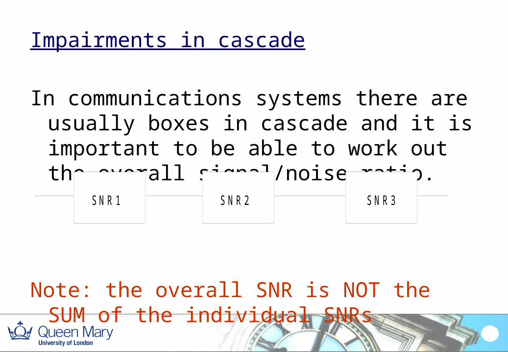
Impairments in cascade

In communications systems there are usually boxes in cascade and it is important to be able to work out the overall signal/noise ratio.

Note: the overall SNR is NOT the SUM of the individual SNRs

SNR 1 SNR2 SNR3

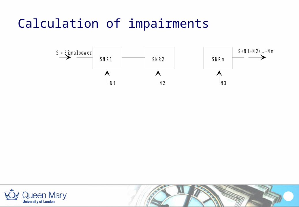
Calculation of impairments

SN R1 SNR2 SNRmS = Signal power

N1 N2 N3

S+N1+N2+.. +Nm

Assume m stages

We have generally that

1010 10or log10 iSNR

iiiii NSNSSNR

or 1010 1010 1 SNRiSNRii SSN

assuming that S is unchanged throughout, the overall signal/noise ratio is:

S

N

S

N

S

Sii

mSNR

i

mSNR

i

m

1

10

1

10

1

10

1

1 101 1

which can be written in dB as usual

74

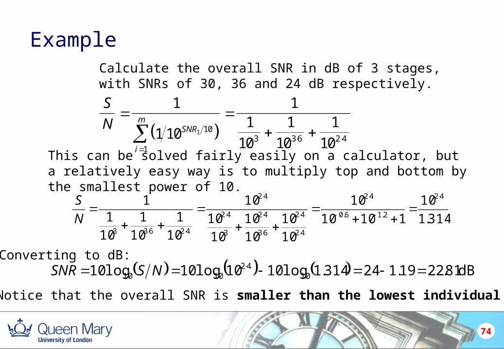
ExampleCalculate the overall SNR in dB of 3 stages, with SNRs of 30, 36 and 24 dB respectively.

S

N SNR

i

m

1

1 10

11

10

1

10

1

101 10

13 3 6 2 4

This can be solved fairly easily on a calculator, but a relatively easy way is to multiply top and bottom by the smallest power of 10.

314.1

10

11010

10

10

10

10

10

10

10

10

10

1

10

1

10

11 42

2.16.0

42

42

42

63

42

3

42

42

42633

N

S

Converting to dB: dB81.2219.124314.1log1010log10log10 10

421010 NSSNR

Notice that the overall SNR is smaller than the lowest individual SNR

Example question

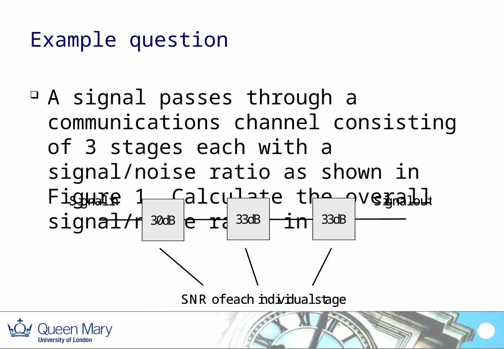
A signal passes through a communications channel consisting of 3 stages each with a signal/noise ratio as shown in Figure 1. Calculate the overall signal/noise ratio in dB.

Signal in Signal out

SNR of each individual stage

33dB 33dB30dBSignal in Signal out

SNR of each individual stage

33dB 33dB30dB

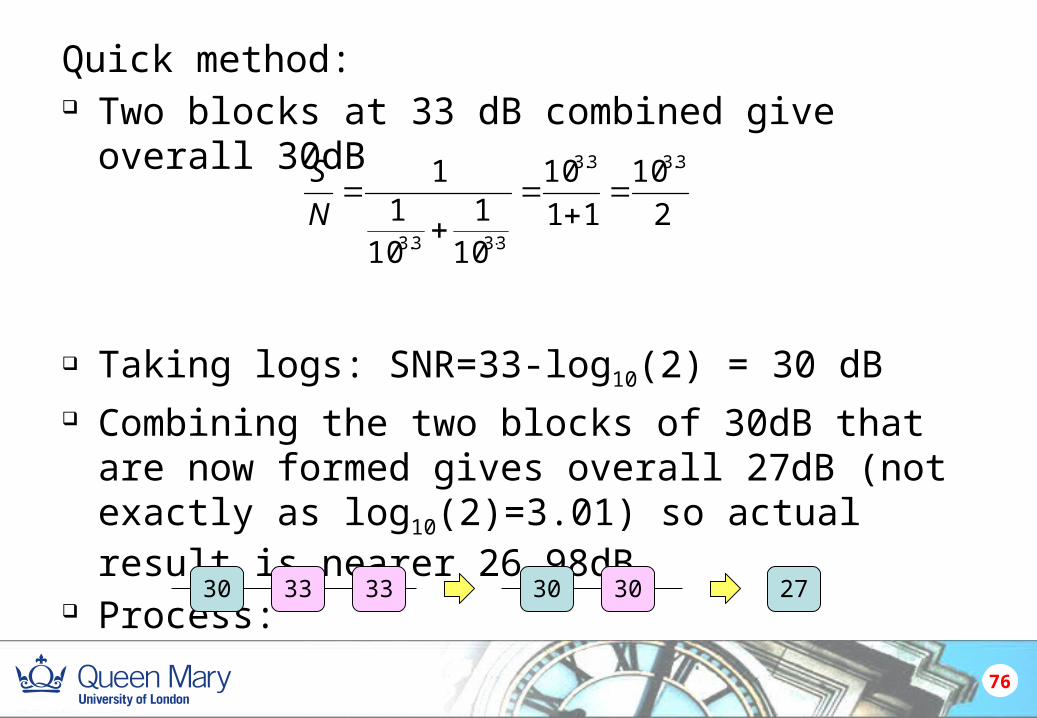
Quick method: Two blocks at 33 dB combined give overall 30dB

Taking logs: SNR=33-log10(2) = 30 dB Combining the two blocks of 30dB that are now formed

gives overall 27dB (not exactly as log10(2)=3.01) so actual result is nearer 26.98dB

Process:

76

2

10

11

10

101

101

1 3.33.3

333.3

N

S

30 33 33 30 30 27

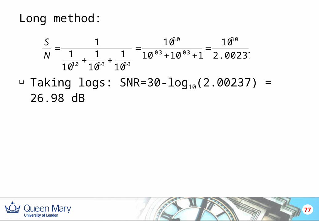
Long method:

Taking logs: SNR=30-log10(2.00237) = 26.98 dB

77

2.002374

10

11010

10

101

101

101

1 0.3

3.03.0

0.3

33330.3

N

S

ARQ

78

79

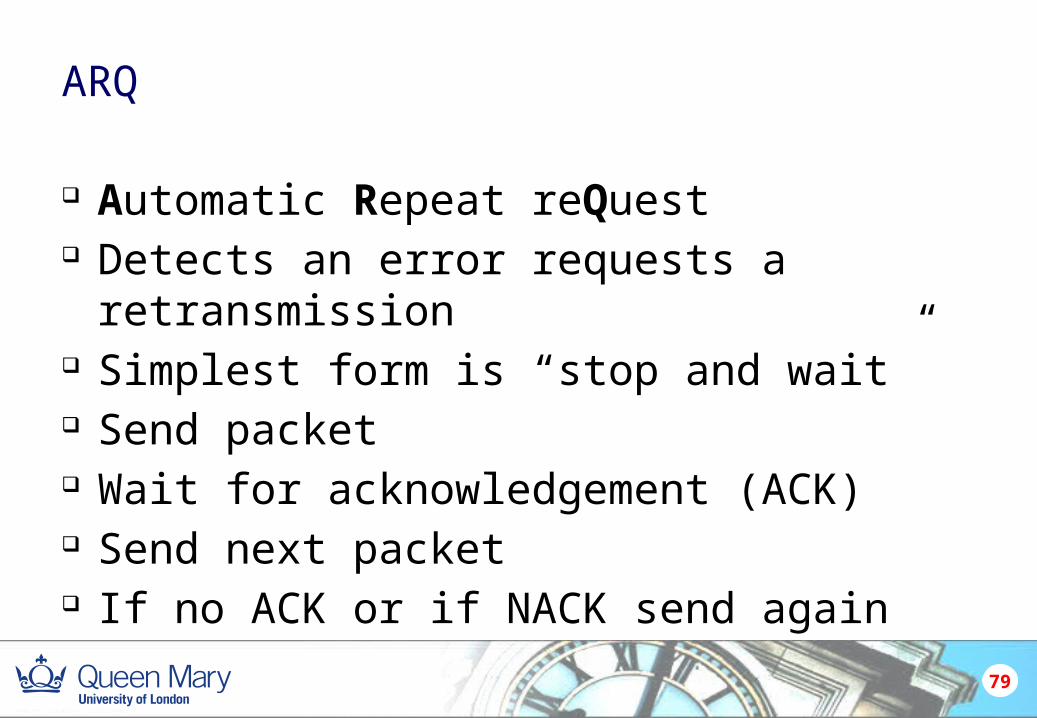
ARQ

Automatic Repeat reQuest Detects an error requests a retransmission Simplest form is “stop and wait” Send packet Wait for acknowledgement (ACK) Send next packet If no ACK or if NACK send again

80

Notation

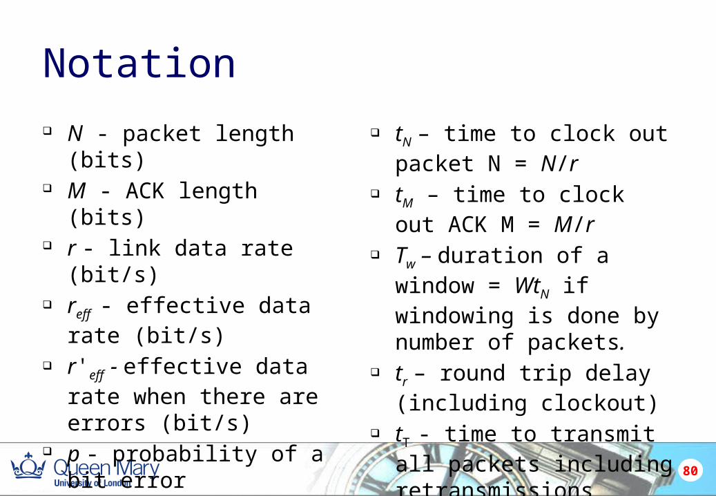
N - packet length (bits) M - ACK length (bits) r - link data rate (bit/s) reff - effective data rate (bit/s) r'eff - effective data rate when

there are errors (bit/s) p - probability of a bit error pwe – probability of a packet

having an error (word error) td - one-way propagation delay

tN – time to clock out packet N = N/r

tM – time to clock out ACK M = M/r

Tw – duration of a window = WtN if windowing is done by number of packets.

tr – round trip delay (including clockout)

tT - time to transmit all packets including retransmissions

Delays

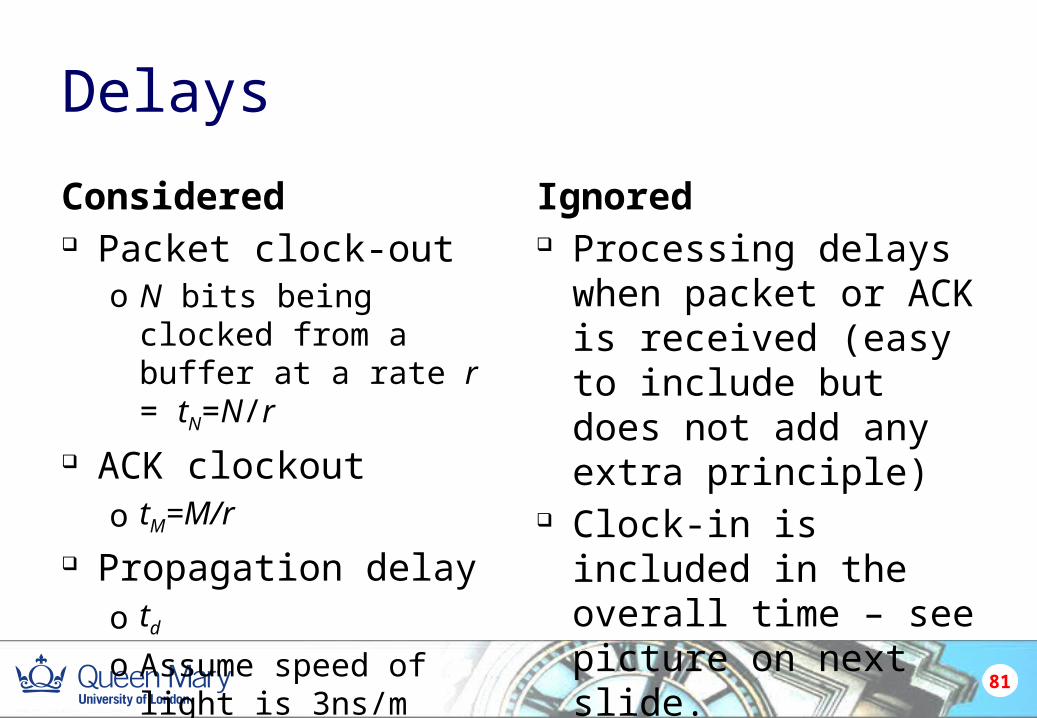
Considered Packet clock-out

o N bits being clocked from a buffer at a rate r = tN=N/r

ACK clockouto tM=M/r

Propagation delayo td

o Assume speed of light is 3ns/m

Ignored Processing delays when

packet or ACK is received (easy to include but does not add any extra principle)

Clock-in is included in the overall time – see picture on next slide.

81

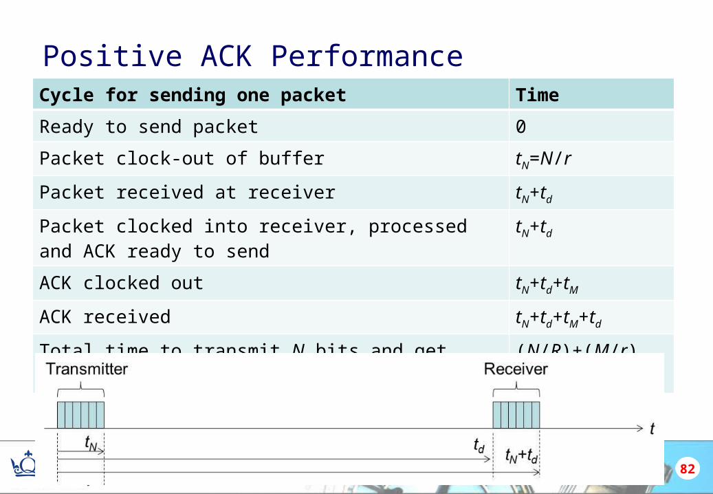
Positive ACK PerformanceCycle for sending one packet Time

Ready to send packet 0

Packet clock-out of buffer tN=N/r

Packet received at receiver tN+td

Packet clocked into receiver, processed and ACK ready to send

tN+td

ACK clocked out tN+td+tM

ACK received tN+td+tM+td

Total time to transmit N bits and get acknowledgement (N/R)+(M/r)+2td=tr

82

83

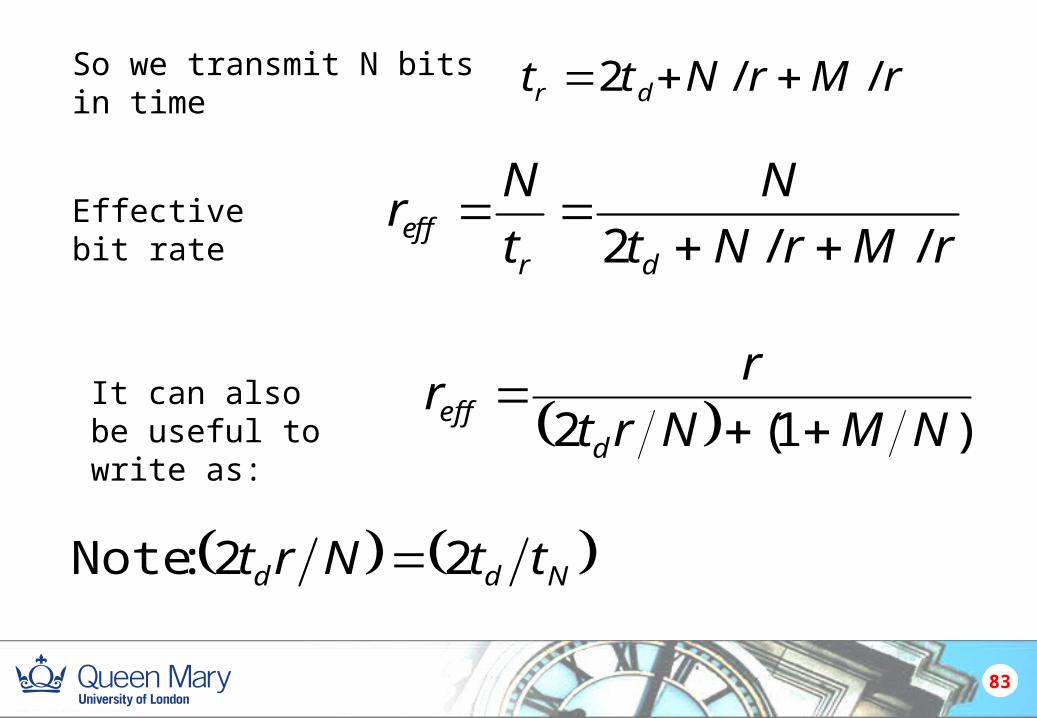
rMrNtt dr //2

Ndd ttNrt 22 :Note

Effective bit rate

So we transmit N bits in time

rMrNt

N

t

Nr

dreff //2

It can also be useful to write as: )1(2 NMNrt

rr

deff

84

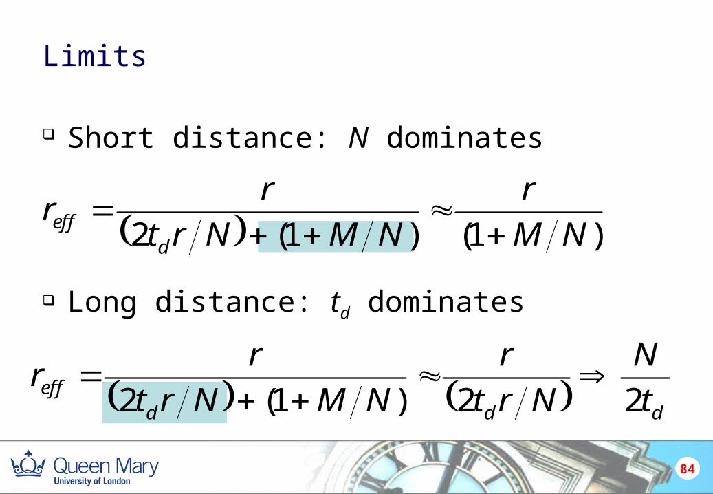
Limits

Short distance: N dominates

Long distance: td dominates

)1()1(2 NM

r

NMNrt

rr

deff

dddeff t

N

Nrt

r

NMNrt

rr

22)1(2

85

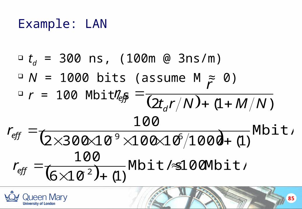
Example: LAN

td = 300 ns, (100m @ 3ns/m) N = 1000 bits (assume M ≈ 0) r = 100 Mbit/s )1(2 NMNrt

rr

deff

Mbit/s)1(100010100103002

10069

effr

Mbit/s 100 Mbit/s)1(106

1002

effr

86

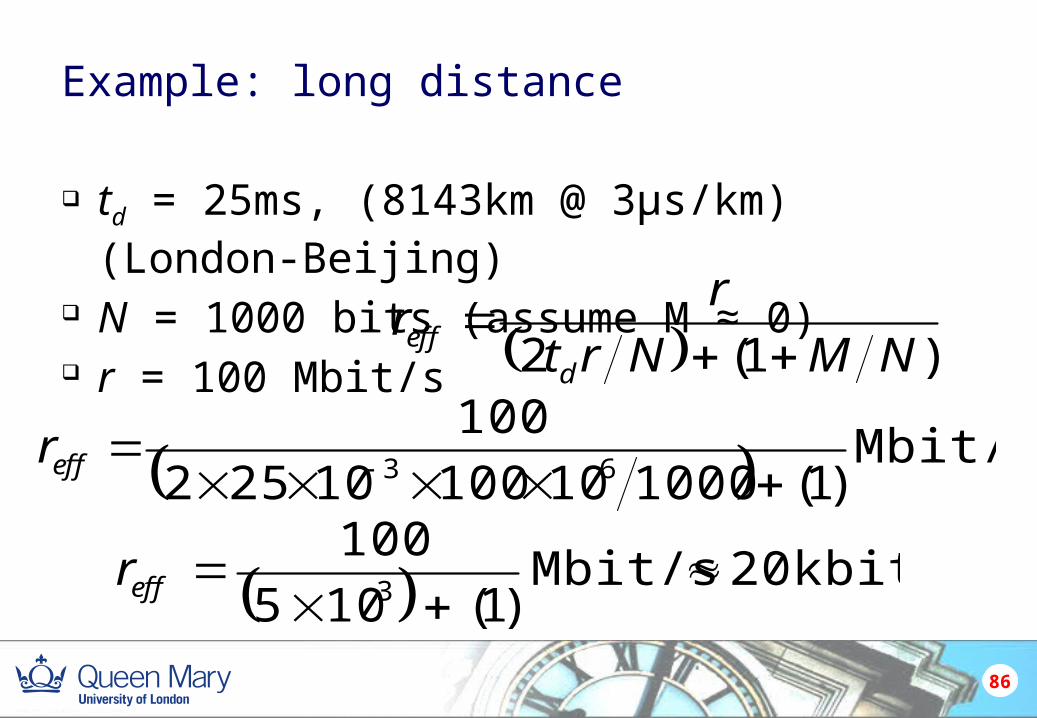
Example: long distance

td = 25ms, (8143km @ 3μs/km) (London-Beijing) N = 1000 bits (assume M ≈ 0) r = 100 Mbit/s )1(2 NMNrt

rr

deff

Mbit/s)1(10001010010252

10063

effr

20kbit/sMbit/s)1(105

1003

effr

87

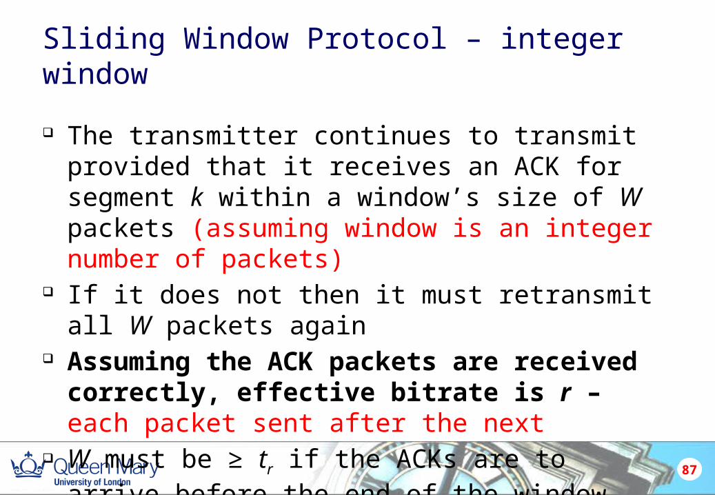
Sliding Window Protocol – integer window

The transmitter continues to transmit provided that it receives an ACK for segment k within a window’s size of W packets (assuming window is an integer number of packets)

If it does not then it must retransmit all W packets again Assuming the ACK packets are received correctly,

effective bitrate is r – each packet sent after the next W must be ≥ tr if the ACKs are to arrive before the end of

the window.

… …

Window for 4

Window for 3

Window for 2 ACK 2

Window for 1. ACK 1

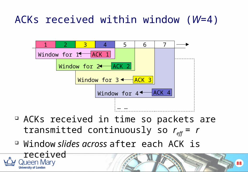
ACKs received within window (W=4)

ACKs received in time so packets are transmitted continuously so reff = r

Window slides across after each ACK is received

88

21 3 4 5 6 7

ACK 3

ACK 4

…. ……

Window for 3

Window for 2 reset and contents resentWindow for 2 – no ACK

Window for 1. ACK 1

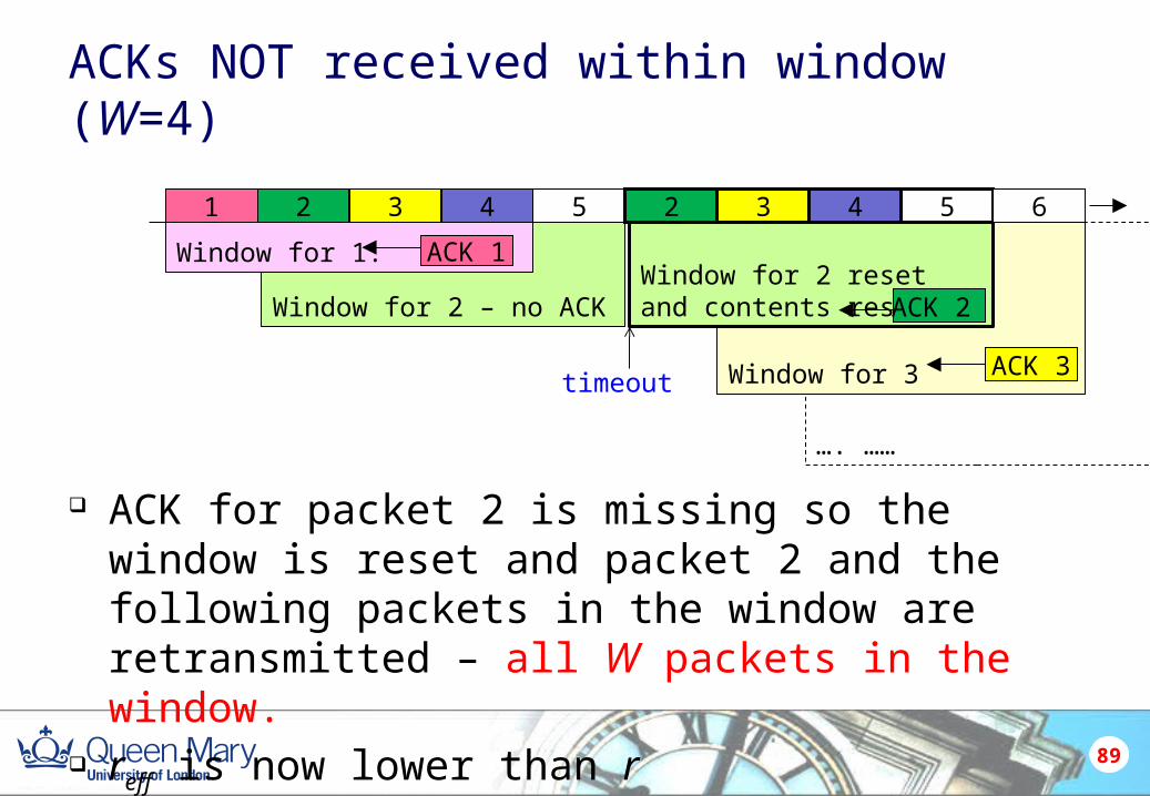
ACKs NOT received within window (W=4)

ACK for packet 2 is missing so the window is reset and packet 2 and the following packets in the window are retransmitted – all W packets in the window.

reff is now lower than r

89

21 3 4 5

ACK 2

2 3 4 5 6

ACK 3timeout

90

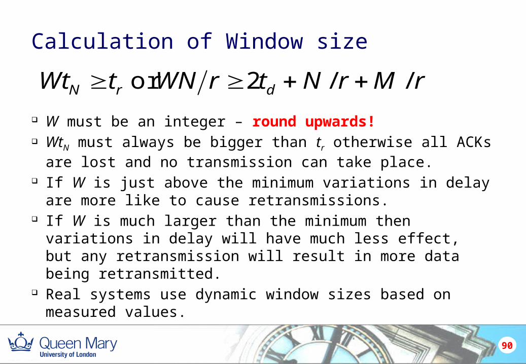
Calculation of Window size

W must be an integer – round upwards! WtN must always be bigger than tr otherwise all ACKs are lost and

no transmission can take place. If W is just above the minimum variations in delay are more like

to cause retransmissions. If W is much larger than the minimum then variations in delay

will have much less effect, but any retransmission will result in more data being retransmitted.

Real systems use dynamic window sizes based on measured values.

rMrNtrWNtWt drN //2or

…. ……

Window for 3

Window for 2 reset and contents resentWindow for 2 – no ACK

Window for 1. ACK 1

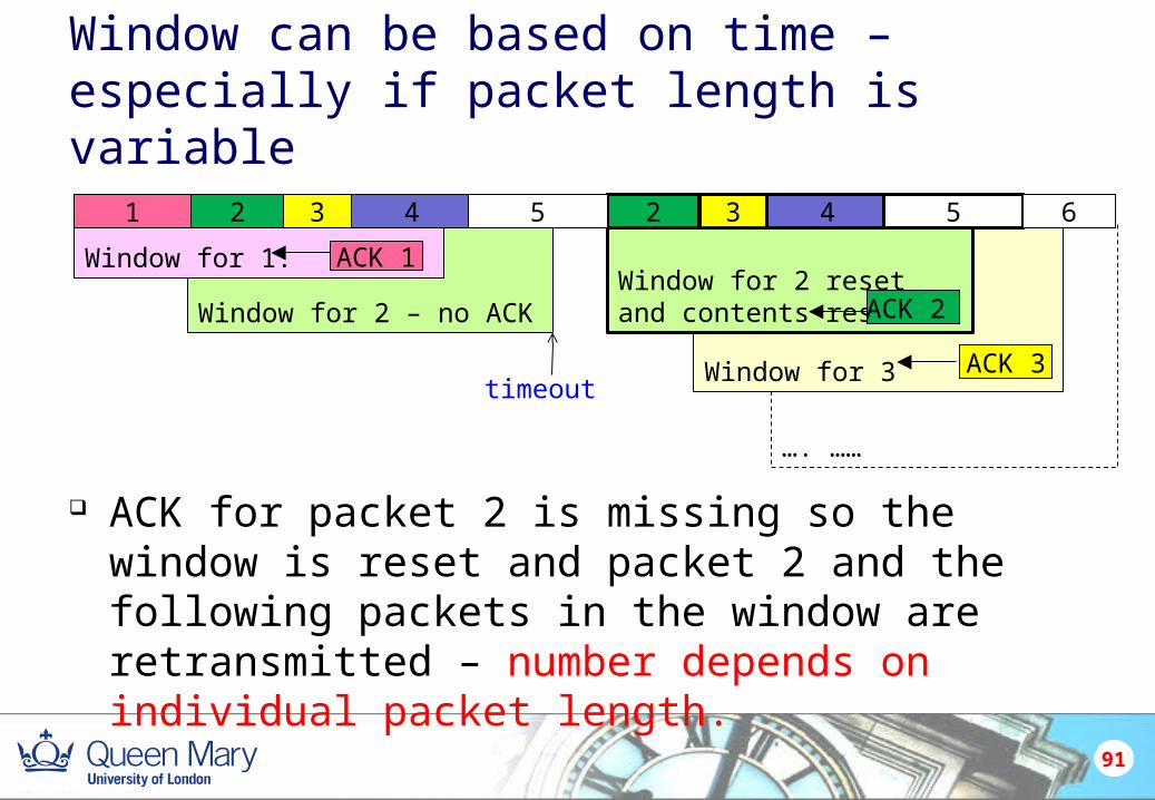
Window can be based on time – especially if packet length is variable

ACK for packet 2 is missing so the window is reset and packet 2 and the following packets in the window are retransmitted – number depends on individual packet length.

91

21 3 4 5

ACK 2

ACK 3

3 4 625

timeout

92

Probability of retransmissions– stop and wait

Bit error probability is p and of a packet error pwe

Assume k packets to transmit. A packet in error will lead to a NACK or no ACK, so

causing a retransmission with probability pwe

This means that we have to transmit k pwe extra packets. Some of the extra packets will have errors and have to be

retransmitted, and so will some of those retransmissions and so on ……. giving a total transmitted of:

........32 wewewe kpkpkpkpackets

93

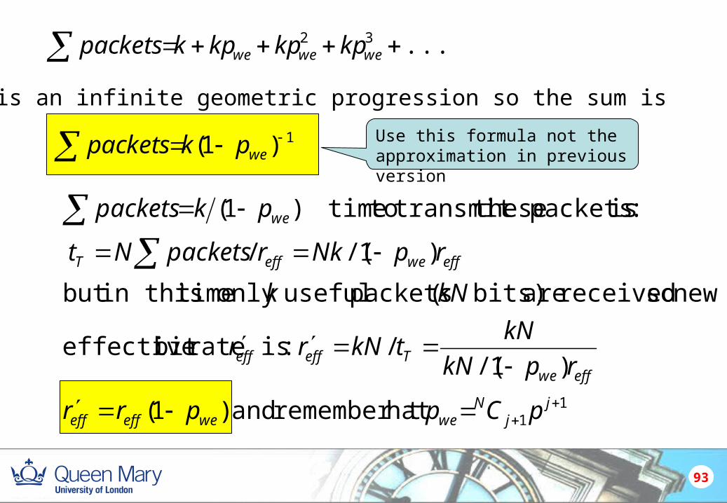
........32 wewewe kpkpkpkpackets

This is an infinite geometric progression so the sum is

1)1( wepkpackets Use this formula not the approximation in previous version

11hat remember t and )1(

)1/(/ :is ratebit effective

new so received are bits) ( packets useful only timein thisbut

)1/(/

:is packets these transmit to time)1(

jj

Nweweeffeff

effweTeffeff

effweeffT

we

pCpprr

rpkN

kNtkNrr

kNk

rpNkrpacketsNt

pkpackets

94

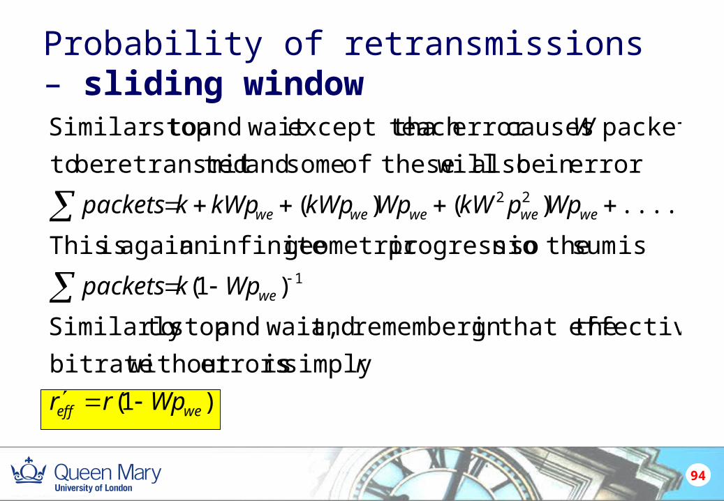
Probability of retransmissions – sliding window

)1(

simply is errors without bitrate

effective that thegrememberin and wait,and stop toSimilarly

)1(

is sum theson progressio geometric infinitean again is This

........)()(

errorin be also will theseof some and tedretransmit be to

packets causeserror each t except tha wait and stop Similar to

1

22

weeff

we

wewewewewe

Wprr

r

Wpkpackets

WppkWWpkWpkWpkpackets

W

95

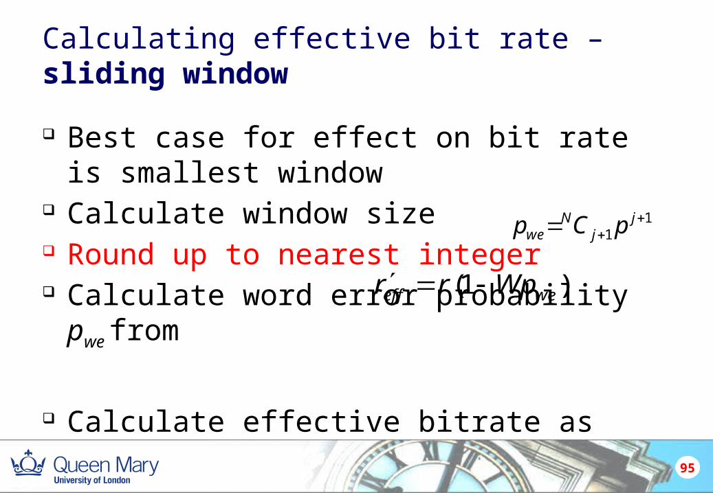
Calculating effective bit rate – sliding window

Best case for effect on bit rate is smallest window Calculate window size Round up to nearest integer Calculate word error probability pwe from

Calculate effective bitrate as

)1( weeff Wprr

11

j

jN

we pCp

Example

N=1000 bits, p=10-4 and W=10

a) No error correction

Pwe = Np = 10-1 so

This means that the error is high enough and the window size large enough that errors in the retransmissions mean that nothing ever gets successfully transmitted.

b) Single bit error correction

Pwe ≈ 0.5(Np)2 = 0.5×10-2 so

96

0)10101()1( 1 rWprr weeff

rrr

rr

Wprr

eff

eff

weeff

95.0)05.01(

)100.5101(

)1(2-

Single bit error correction is very effective in improving rate

97

Window for packet 2

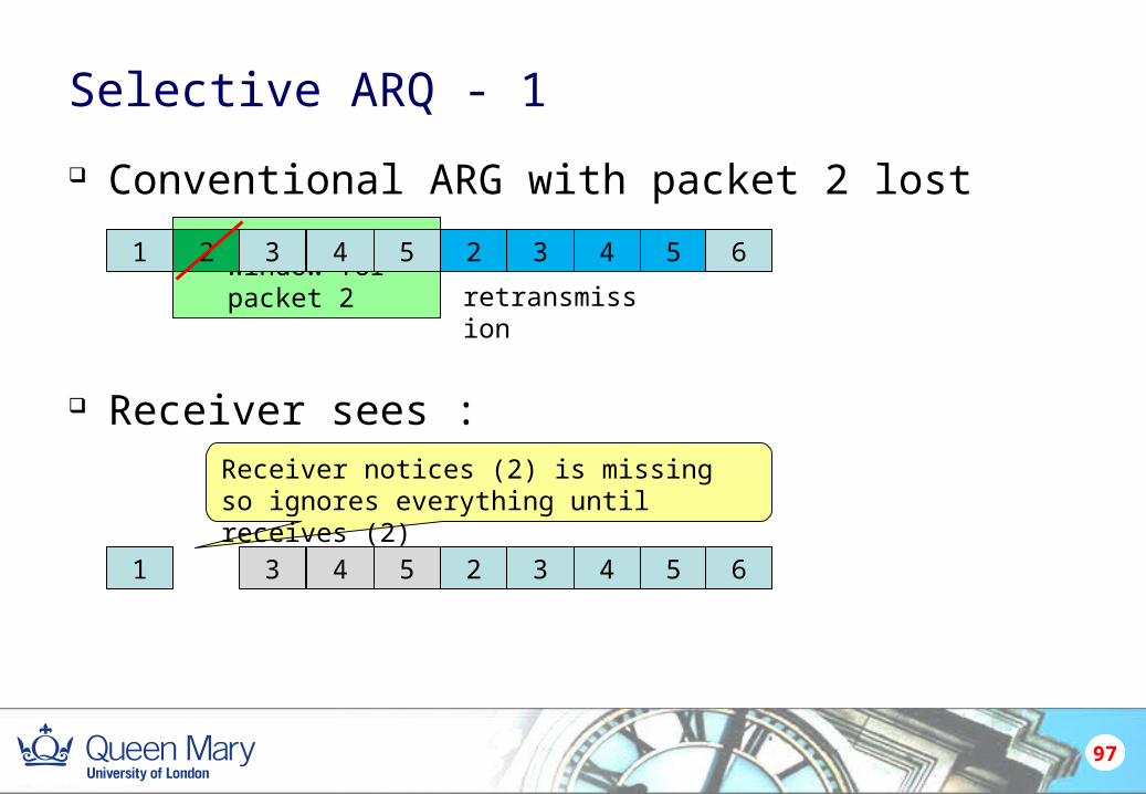
Selective ARQ - 1

Conventional ARG with packet 2 lost

Receiver sees :

1 2 3 4 5 2 3 4 5 6

retransmission

1 3 4 5 2 3 4 5 6

Receiver notices (2) is missing so ignores everything until receives (2)

98

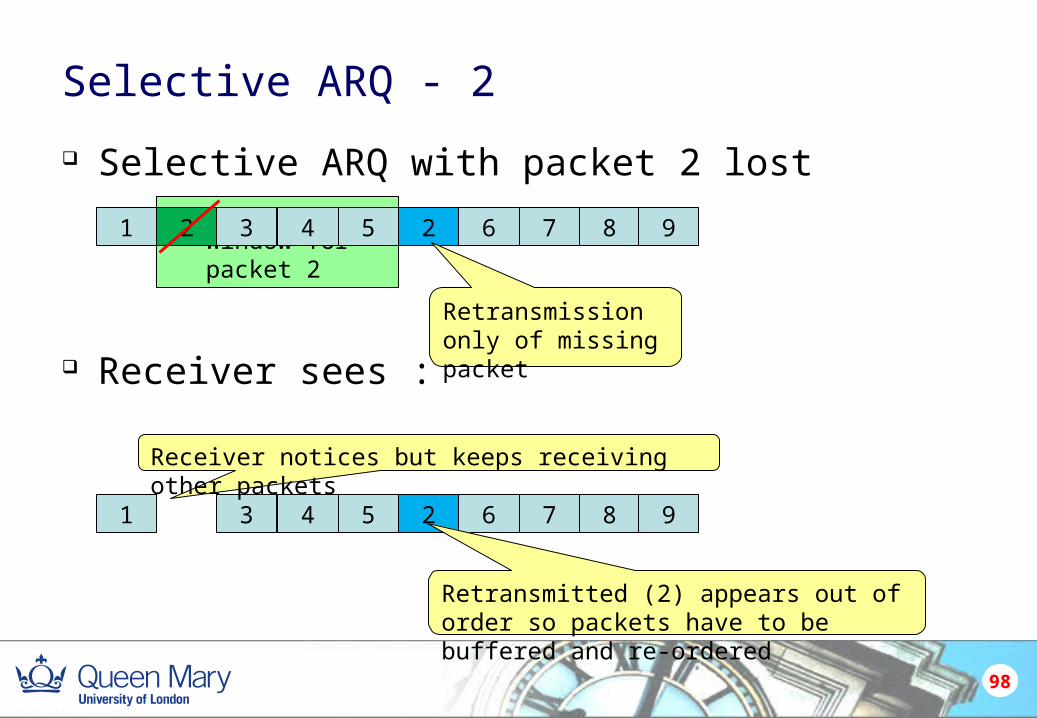
Window for packet 2

Selective ARQ - 2

Selective ARQ with packet 2 lost

Receiver sees :

1 2 3 4 5 2 6 7 8 9

1 3 4 5 2 6 7 8 9

Receiver notices but keeps receiving other packets

Retransmission only of missing packet

Retransmitted (2) appears out of order so packets have to be buffered and re-ordered

99

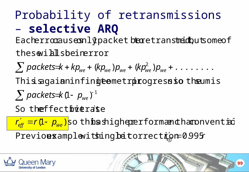
Probability of retransmissions – selective ARQ

rr

prr

i

pkpackets

pkppkpkpkpackets

eff

weeff

we

wewewewewe

995.0 correctionbit single with example Previous

alconvention than eperformanchigher has thisso )1(

s bitrate effective theSo

)1(

is sum theson progressio geometric infinitean again is This

........)()(

errorin be also willthese

of somebut ted,retransmit be packet to 1only causeserror Each

1

2

When window is a delay

Similar approach but more complicated Use TW instead of W Have to calculate the delay in sending a new window and

the number of packets in that window based on the average packet length if packets are different.

For this course assume packets are same length and the window size is integer

100

ERROR CONTROL CODING

Error control coding

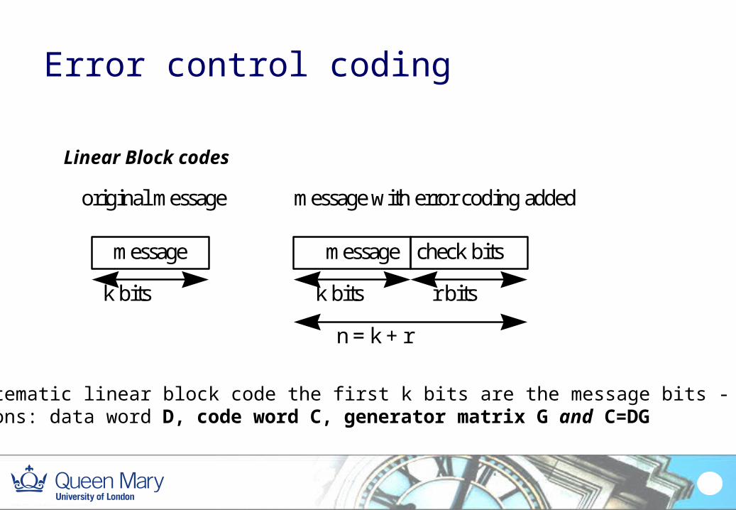
Linear Block codes

message message check bits

k bits k bits r bits

n = k + r

original message message with error coding added

In a systematic linear block code the first k bits are the message bits - as aboveDefinitions: data word D, code word C, generator matrix G and C=DG

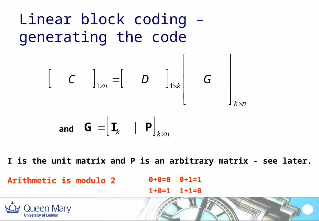
Linear block coding – generating the code

G I Pk k n

|

C D Gn k

k n

1 1

and

I is the unit matrix and P is an arbitrary matrix - see later.

Arithmetic is modulo 2 0+0=0 0+1=1

1+0=1 1+1=0

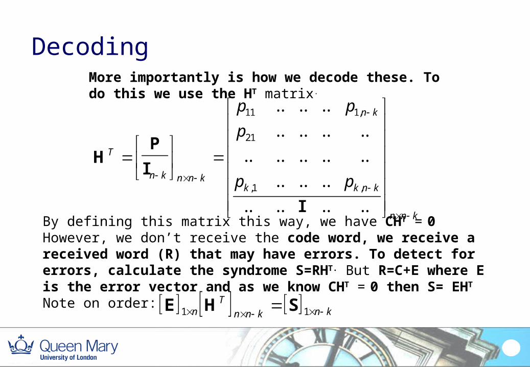
DecodingMore importantly is how we decode these. To do this we use the HT matrix.

By defining this matrix this way, we have CHT = 0However, we don’t receive the code word, we receive a received word (R) that may have errors. To detect for errors, calculate the syndrome S=RHT. But R=C+E where E is the error vector and as we know CHT = 0 then S= EHT

Note on order:

HP

I

I

T

n k n n k

n k

k k n k

n n k

p p

p

p p

11 1

21

1

.. .. ..

.. .. .. ..

.. .. .. .. ..

.. .. ..

.. .. .. ..

,

, ,

E H S1 1 nT

n n k n k

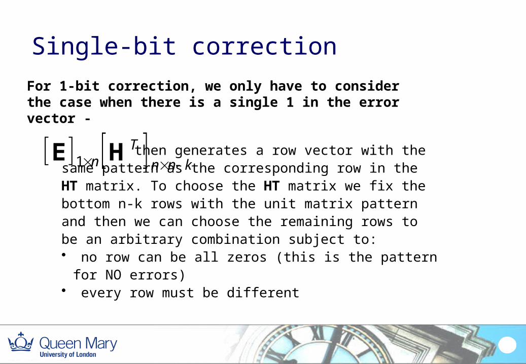
Single-bit correction

For 1-bit correction, we only have to consider the case when there is a single 1 in the error vector -

E H1 nT

n n k then generates a row vector with the same pattern as the corresponding row in the HT matrix. To choose the HT matrix we fix the bottom n-k rows with the unit matrix pattern and then we can choose the remaining rows to be an arbitrary combination subject to:• no row can be all zeros (this is the pattern for NO errors)• every row must be different

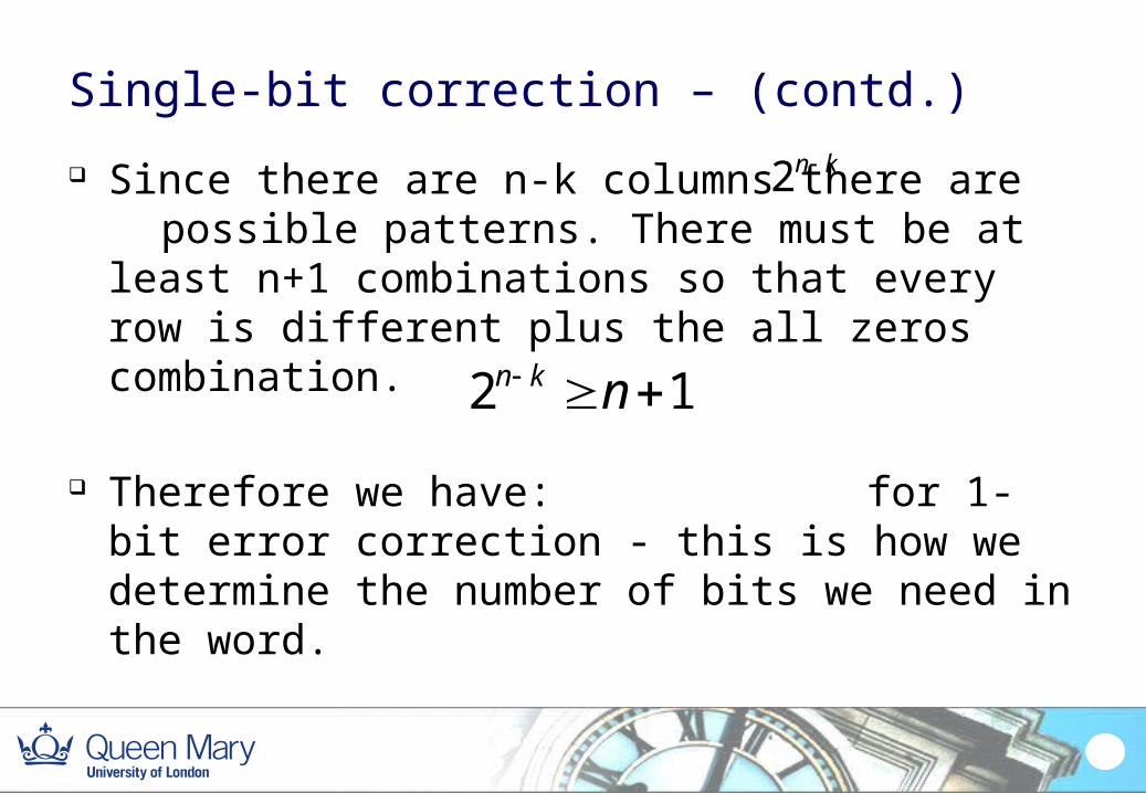
Single-bit correction – (contd.)

Since there are n-k columns there are possible patterns. There must be at least n+1 combinations so that every row is different plus the all zeros combination.

Therefore we have: for 1-bit error correction - this is how we determine the number of bits we need in the word.

2n k

12 nkn

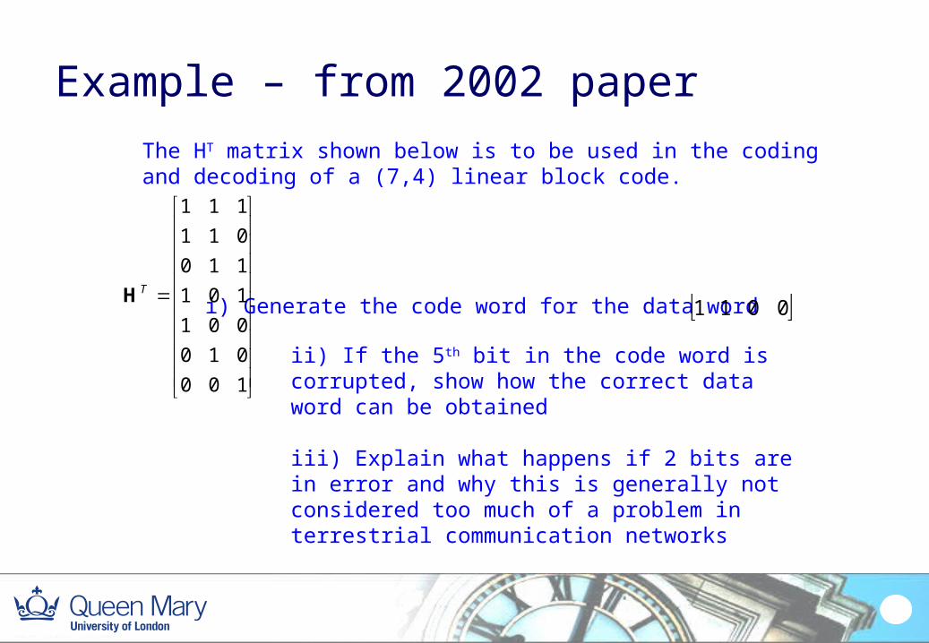
Example – from 2002 paper

The HT matrix shown below is to be used in the coding and decoding of a (7,4) linear block code.

100

010

001

101

110

011

111

TH i) Generate the code word for the data word 0011

ii) If the 5th bit in the code word is corrupted, show how the correct data word can be obtained

iii) Explain what happens if 2 bits are in error and why this is generally not considered too much of a problem in terrestrial communication networks

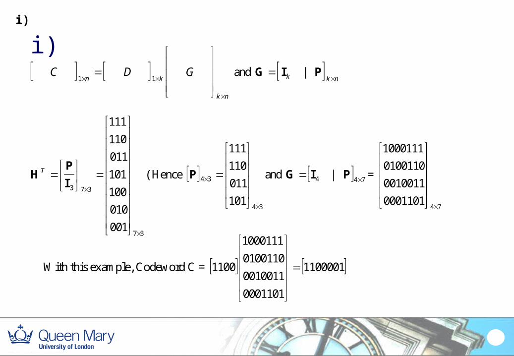
i) C D G

n k

k n

1 1

and G I Pk k n

|

37

373

001

010

100

101

011

110

111

I

PHT ( Hence

34

34

101

011

110

111

P and 744 | PIG =

740001101

0010011

0100110

1000111

With this example, Codeword C = 1100001

0001101

0010011

0100110

1000111

1100

i)

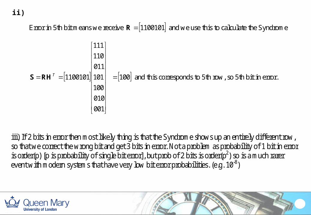
Error in 5th bit means we receive 1100101R and we use this to calculate the Syndrome

100

001

010

100

101

011

110

111

1100101

TRHS and this corresponds to 5th row, so 5th bit in error.

iii) If 2 bits in error then most likely thing is that the Syndrome shows up an entirely different row, so that we correct the wrong bit and get 3 bits in error. Not a problem as probability of 1 bit in error is order(p) [p is probability of single bit error], but prob of 2 bits is order(p2) so is a much rarer event with modern systems that have very low bit error probabilities. (e.g. 10-8)

ii)

From 2006 paper

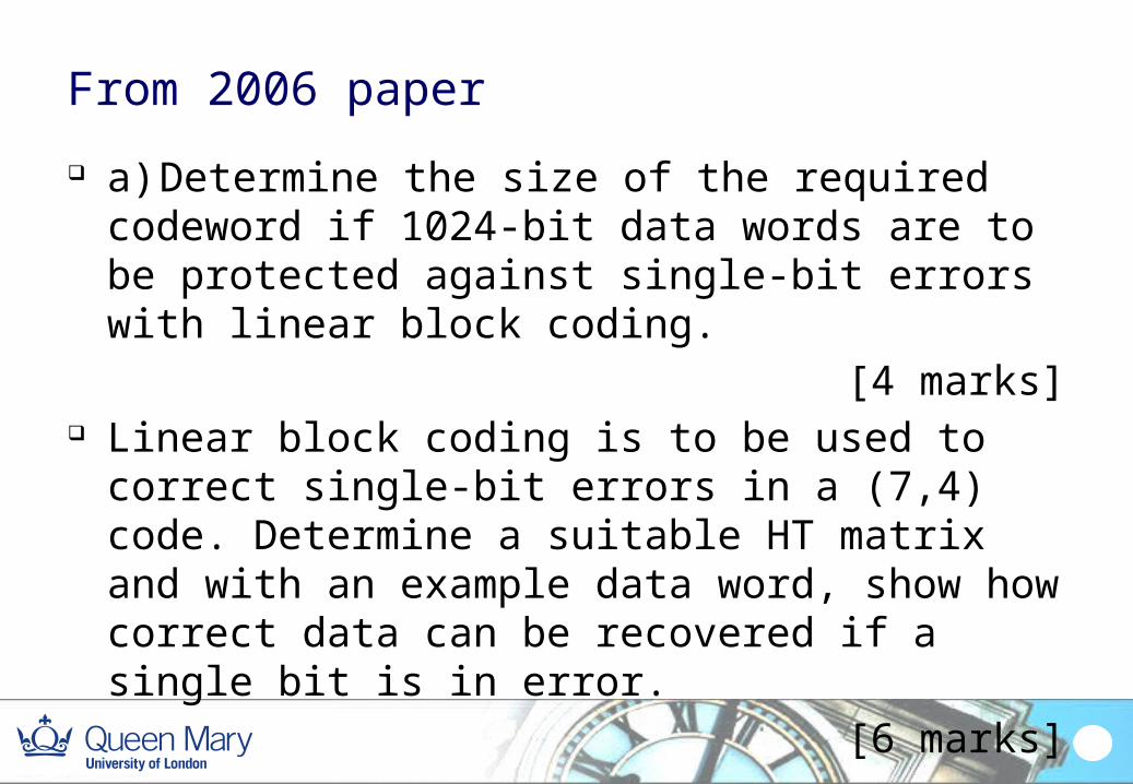
a) Determine the size of the required codeword if 1024-bit data words are to be protected against single-bit errors with linear block coding.

[4 marks] Linear block coding is to be used to correct single-bit

errors in a (7,4) code. Determine a suitable HT matrix and with an example data word, show how correct data can be recovered if a single bit is in error.

[6 marks]

From 2005 paper

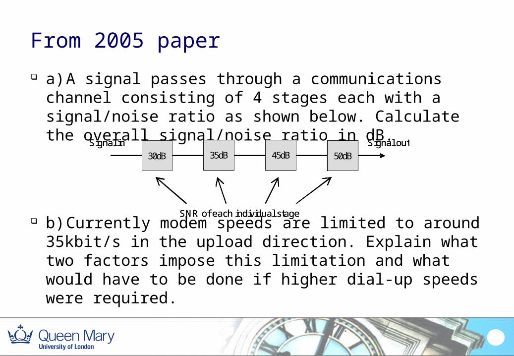
a) A signal passes through a communications channel consisting of 4 stages each with a signal/noise ratio as shown below. Calculate the overall signal/noise ratio in dB.

b) Currently modem speeds are limited to around 35kbit/s in the upload direction. Explain what two factors impose this limitation and what would have to be done if higher dial-up speeds were required.

Signal in Signal out

SNR of each individual stage

35dB 45dB 50dB30dBSignal in Signal out

SNR of each individual stage

35dB 45dB 50dB30dB

Fom 2005 paper

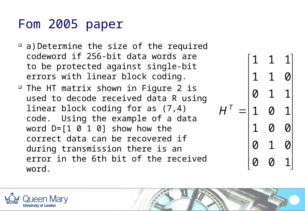
a) Determine the size of the required codeword if 256-bit data words are to be protected against single-bit errors with linear block coding.

The HT matrix shown in Figure 2 is used to decode received data R using linear block coding for as (7,4) code. Using the example of a data word D=[1 0 1 0] show how the correct data can be recovered if during transmission there is an error in the 6th bit of the received word.

100

010

001

101

110

011

111

TH

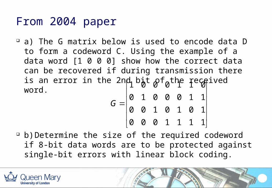
From 2004 paper

a) The G matrix below is used to encode data D to form a codeword C. Using the example of a data word [1 0 0 0] show how the correct data can be recovered if during transmission there is an error in the 2nd bit of the received word.

b) Determine the size of the required codeword if 8-bit

data words are to be protected against single-bit errors with linear block coding.

1111000

1010100

1100010

0110001

G

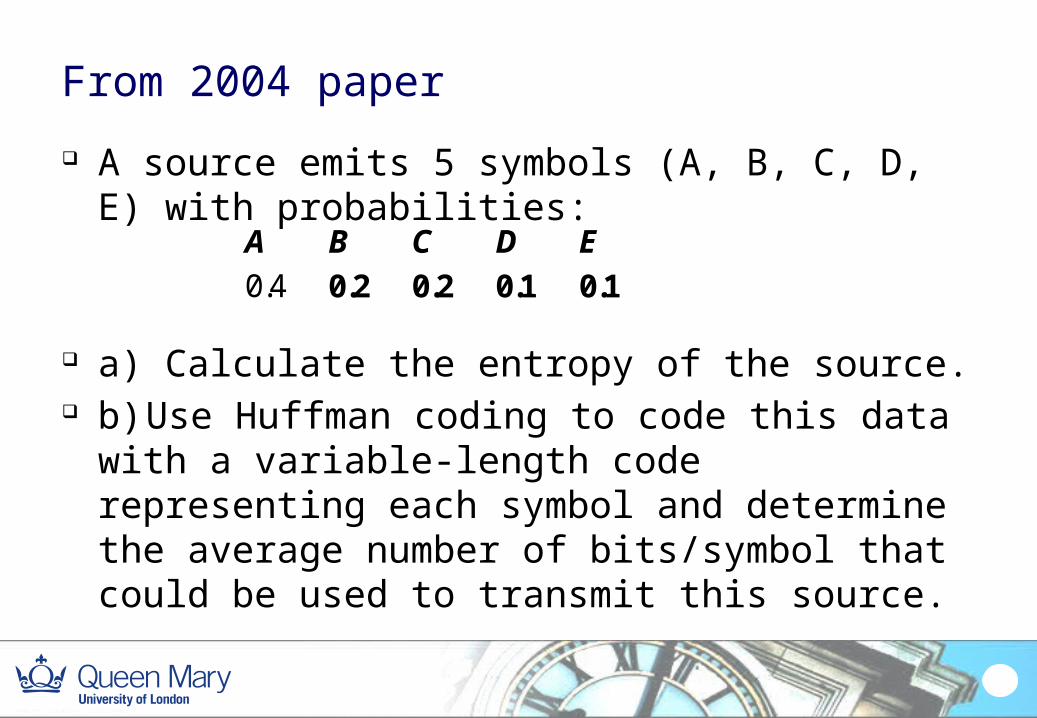
From 2004 paper

A source emits 5 symbols (A, B, C, D, E) with probabilities:

a) Calculate the entropy of the source. b) Use Huffman coding to code this data with a

variable-length code representing each symbol and determine the average number of bits/symbol that could be used to transmit this source.

A B C D E 0.4 0.2 0.2 0.1 0.1

Cyclic codes

Look-up tables get very big for large codewords – not easy to implement in hardware.

Cyclic codes easy to implement using shift registers Work using the principle of cyclic polynomials Every code member is a cyclic shift of another

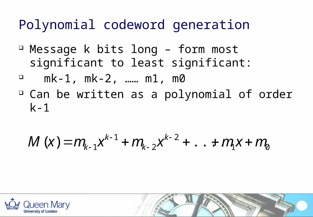
Polynomial codeword generation

Message k bits long – form most significant to least significant:

mk-1, mk-2, …… m1, m0 Can be written as a polynomial of order k-1

012

21

1 .....)( mxmxmxmxM kk

kk

Generating codeword

Use generator polynomial P(x) Multiply (bit shift) M(x) by order of P(x) to create M’(x) Divide M’(x) by P(x) Add remainder of division to M’(x) to make C(x) Notes:

o quotient is discardedo generator is chosen carefully to cover the errors expected