WAN MOHAMAD DASUQI BIN WAN MA’SOR - Welcome to …umpir.ump.edu.my/1914/1/Wan_Mohamad_Dasuqi_Wan_Ma'sor_(_CD_4943_).pdf · WAN MOHAMAD DASUQI BIN WAN MA’SOR Report submitted in

SIMULATION OF BUBBLES RISE IN CAVITY USING LATTICE BOLZTMANN

METHOD

WAN MOHAMAD DASUQI BIN WAN MA’SOR

Report submitted in partial fulfilment of the requirements

for the award of the degree of

Bachelor of Mechanical Engineering

Faculty of Mechanical Engineering

UNIVERSITI MALAYSIA PAHANG

DECEMBER 2010

ii

SUPERVISOR’S DECLARATION

I hereby declare that I have checked this project and in my opinion, this project is

adequate in terms of scope and quality for the award of the degree of Bachelor of

Mechanical Engineering.

Signature:

Name of Supervisor: MUHAMAD ZUHAIRI BIN SULAIMAN

Position: LECTURER

Date: 6/12/2010

iii

STUDENT’S DECLARATION

I hereby declare that the work in this project is my own except for quotations and

summaries which have been duly acknowledged. The project has not been accepted for

any degree and is not concurrently submitted for award of other degree.

Signature:

Name: WAN MOHAMAD DASUQI B WAN MA’SOR

Id Number: MA07052

Date: 6/12/2010

v

ACKNOWLEDGEMENTS

First of all, I would like to express my heartily gratitude to my research

supervisor, Associate Mr. Muhamad Zuhairi bin Sulaiman for his guidance, advices,

efforts, supervision and enthusiasm given throughout for the progress of this research.

In preparing this thesis, I was in contact with many people, lecturers, and

training engineers. They have contributed towards my understanding and thoughts.

Without their continued support and interest, this thesis would not have been the same

as presented here.

I would like to express my sincere appreciation to my parents for their support to

me all this year. Without them, I would not be able to complete this research. Besides

that, I would like to thank my course mates and my friends especially my section M06

for their help, assistance and support and encouragement.

vi

ABSTRACT

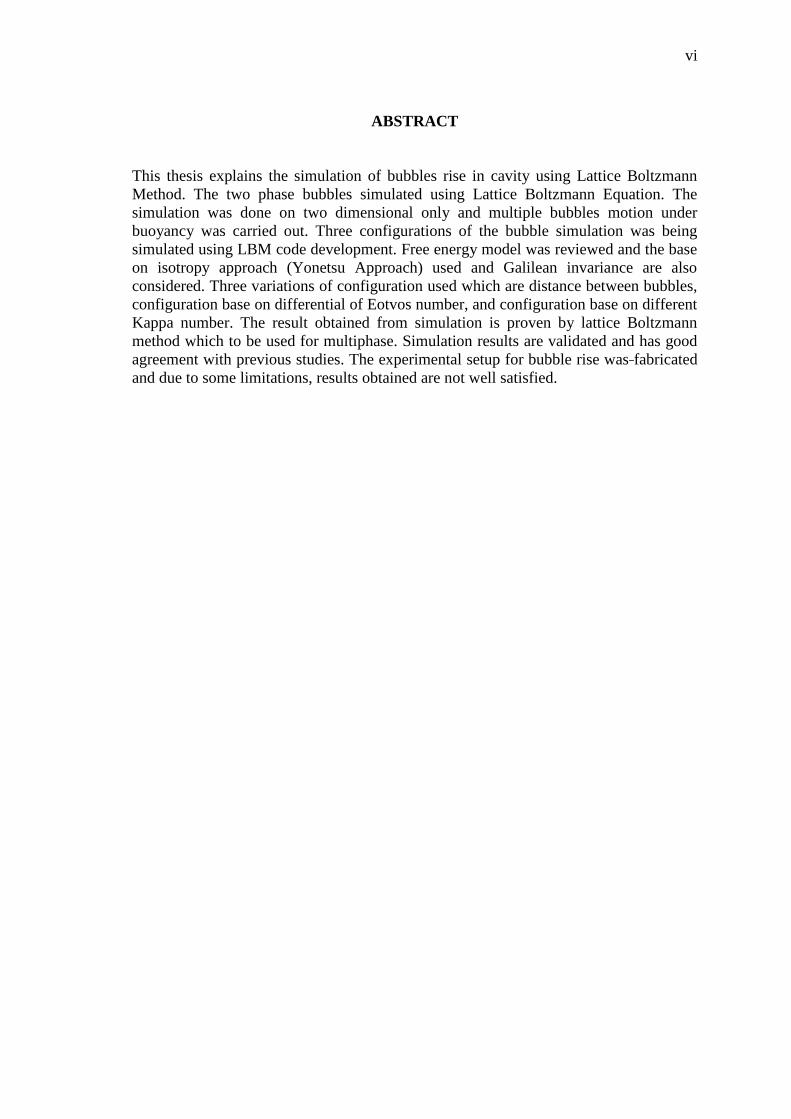
This thesis explains the simulation of bubbles rise in cavity using Lattice Boltzmann

Method. The two phase bubbles simulated using Lattice Boltzmann Equation. The

simulation was done on two dimensional only and multiple bubbles motion under

buoyancy was carried out. Three configurations of the bubble simulation was being

simulated using LBM code development. Free energy model was reviewed and the base

on isotropy approach (Yonetsu Approach) used and Galilean invariance are also

considered. Three variations of configuration used which are distance between bubbles,

configuration base on differential of Eotvos number, and configuration base on different

Kappa number. The result obtained from simulation is proven by lattice Boltzmann

method which to be used for multiphase. Simulation results are validated and has good

agreement with previous studies. The experimental setup for bubble rise was fabricated

and due to some limitations, results obtained are not well satisfied.

vii

ABSTRAK

Thesis ini menerangkan mengenai kajian terhadap simulasi buih yang naik dari kaviti

melalui aliran dua fasa berdasarkan kaedah Lattice Boltzmann. Simulasi buih ini

berasaskan dari persamaan kaedah Lattice Boltzmann. Simulasi ini hanya dilakukan

dalam dua dimensi analisis sahaja dan pada masa yang sama apungan ke atas

pergerakan buih berganda akan dapat dipelajari. Tiga jenis rupa bentuk simulasi buih

yang menggunakan LBM akan di simulasikan melalui perisian Visual C++. Model

tenaga bebas akan di tinjau kembali berdasarkan model yang terbaru yang berasas

pendekatan isotropik( Pendekatan Yonetsu). Ketidaksamaan Galliean juga akan di

pertimbangkan. Rupa bentuk yang disimulasikan di dalam thesis ini antaranya adalah

rupa bentuk disebabkan pendekatan jarak diantara buih, rupa bentuk yang disebabkan

perbezaan nombor Eotvos, dan terakhir sekali disebabkan perbezaan nombor Kappa.

Keputusan yang diperolehi melalui simulasi ini telah dibuktikan melalui persamaan

Lattice Boltzmann dan digunakan untuk dua fasa. Keputusan simulasi ini di perakui sah

dan mendapat persetujuan yang baik dengan pembelajaran sebelum ini. Eksperimen

penaikan buih secara manual juga telah dicipta dan bergantung ke atas tahap yang

terhad, keputusan yang diperolehi masih belum sempurna.

viii

TABLE OF CONTENT

Page

CHAPTER 1 INTRODUCTION

1.2 Background of Lattice Boltzmann Method 2

1.3 Problem Statement 4

1.4 Objectives 4

1.5 Project Scope 5

CHAPTER 2 LITERATURE REVIEW

2.2 Lattice Boltzmann Method 7

2.3 Kinetic Theory 9

2.4 First Order Distribution Function 9

2.5 LBM Framework and Equations 12

2.6 Multiphase Lattice Boltzmann Method 15

2.7 Van De Waals Fluid 17

2.8 Maxwell equal area construction 20

2.9 Yonetsu's Approach 21

SUPERVISOR’S DECLARATION ii

STUDENT’S DECLARATION iii

ACKNOWLEDGEMENTS v

ABSTRACT vi

ABSTRAK vii

TABLE OF CONTENTS viii

LIST OF TABLES xi

LIST OF FIGURES xii

LIST OF ABBREVIATIONS xiii

LIST OF APPENDICES xiv

ix

CHAPTER 3 METHODOLOGY

3.2 Flow Chart 24

3.3 Physical Properties 26

3.4 Code Development 27

3.5 Initial Condition 28

3.6 Advection 28

3.7 Collision 31

3.8 Boundary Condition 32

3.8.1 Bounce back Boundaries 33

3.9 Output 34

3.10 Convergent 35

3.10.1 Effect of Eotvos Number 35

3.10.2 Effect of Kappa number 38

3.10.3 Effect of Distance Increment 39

3.11 Experimental Setup 39

CHAPTER 4 RESULTS AND DISCUSSION

4.2 Effect by Distance Increment between Bubble (Case 1) 43

4.2.1Discussion (Case 1) 44

4.3 Effect by Eotvos number (Case 2) 45


4.4 Effect of kappa number ,𝜅 (Case 3) 47


4.5 Experimental Result 49

CHAPTER 5 CONCLUSION AND RECOMMENDATION

5.2 Conclusion 53

5.3 Recommendation 54

x

REFERENCES 55

APPENDIX A 56

APPENDIX B 57

APPENDIX C 58

APPENDIX D 59

APPENDIX E1 60

APPENDIX E2 61

APPENDIX E3 62

APPENDIX F1 63

APPENDIX F2 64

APPENDIX F3 65

APPENDIX G1 66

APPENDIX G2 67

APPENDIX G3 68

APPENDIX H 69

APPENDIX I1 70

APPENDIX I2 71

APPENDIX I3 72

APPENDIX J1 73

APPENDIX J2 74

APPENDIX J3 75

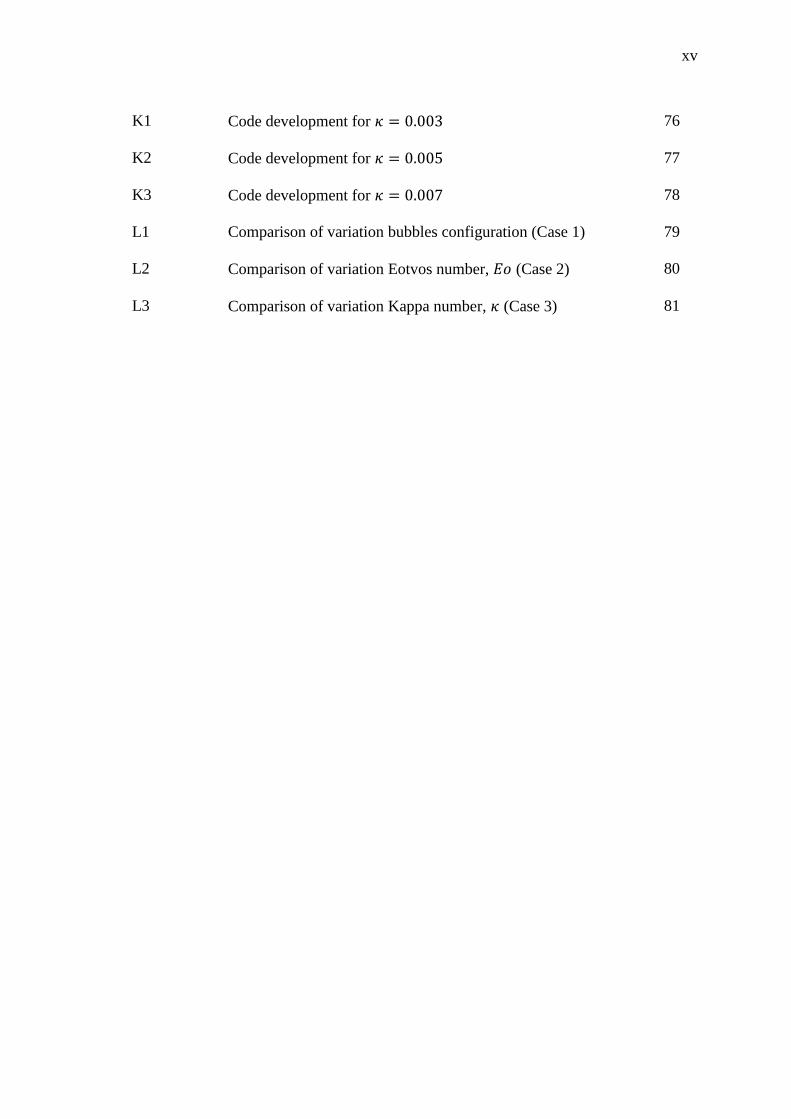
APPENDIX K1 76

APPENDIX K2 77

APPENDIX K3 78

APPENDIX L1 79

APPENDIX L2 80

APPENDIX L3 81

xi

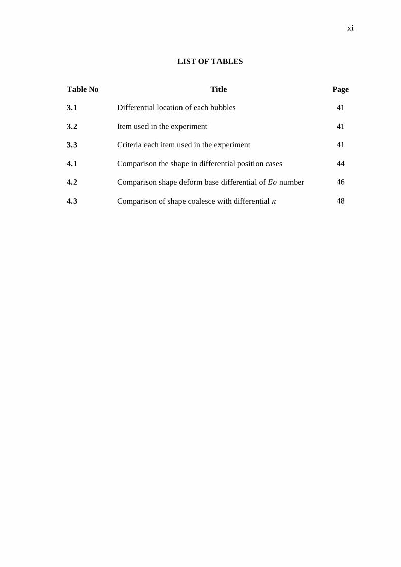
LIST OF TABLES

Table No

Title Page

3.1 Differential location of each bubbles

41

3.2 Item used in the experiment

41

3.3 Criteria each item used in the experiment

41

4.1 Comparison the shape in differential position cases

44

4.2 Comparison shape deform base differential of 𝐸𝑜 number

46

4.3 Comparison of shape coalesce with differential 𝜅 48

xii

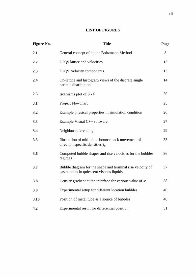
LIST OF FIGURES

Figure No.

Title Page

2.1 General concept of lattice Boltzmann Method

8

2.2 D2Q9 lattice and velocities.

13

2.3 D2Q9 velocity components

13

2.4 On-lattice and histogram views of the discrete single

particle distribution

14

2.5 Isotherms plot of 𝑝 - 𝑉

20

3.1 Project Flowchart

25

3.2 Example physical properties in simulation condition

26

3.3 Example Visual C++ software

27

3.4 Neighbor referencing

29

3.5 Illustration of mid-plane bounce back movement of

direction specific densities 𝑓𝑎

33

3.6 Computed bubble shapes and rise velocities for the bubbles

regimes

36

3.7 Bubble diagram for the shape and terminal rise velocity of

gas bubbles in quiescent viscous liquids

37

3.8 Density gradient at the interface for various value of 𝜿

38

3.9 Experimental setup for different location bubbles

40

3.10 Position of metal tube as a source of bubbles

40

4.2 Experimental result for differential position 51

xiii

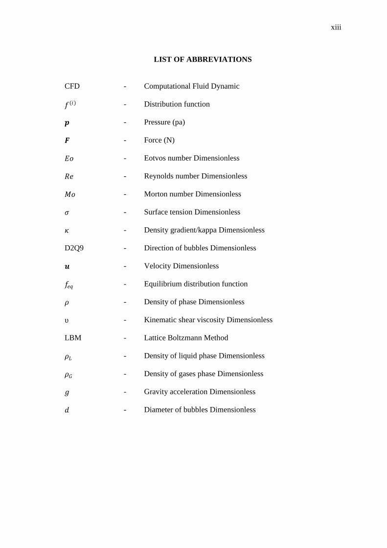
LIST OF ABBREVIATIONS

CFD - Computational Fluid Dynamic

𝑓(𝑖) - Distribution function

𝒑 - Pressure (pa)

𝑭 - Force (N)

𝐸𝑜 - Eotvos number Dimensionless

𝑅𝑒 - Reynolds number Dimensionless

𝑀𝑜 - Morton number Dimensionless

𝜎 - Surface tension Dimensionless

𝜅 - Density gradient/kappa Dimensionless

D2Q9 - Direction of bubbles Dimensionless

𝒖 - Velocity Dimensionless

𝑓𝑒𝑞 - Equilibrium distribution function

𝜌 - Density of phase Dimensionless

ʋ - Kinematic shear viscosity Dimensionless

LBM - Lattice Boltzmann Method

𝜌𝐿 - Density of liquid phase Dimensionless

𝜌𝐺 - Density of gases phase Dimensionless

𝑔 - Gravity acceleration Dimensionless

𝑑 - Diameter of bubbles Dimensionless

xiv

LIST OF APPENDIX

Appendix Title Page

A Sample of output in visual C++ software

56

B AVS express software to show the result

57

C Deformation shape when not coalesce

58

D Deformation shape when can coalesce

59

E1 Deformation shape diagram at location (36160 , 80

160 ,

124160 )

60


160 ,

120160 )

61


160 ,

116160 )

62

F1 Deformation shape diagram at 𝐸𝑜=10

63


64


65

G1 Deformation shape diagram at 𝜅 = 0.003

66


67


68

H Gannt Chart

69

I1 Code development for position (36160 , 80

160 , 124160 )

70


160 , 120160 )

71


160 , 116160 ).

72

J1 Code development for 𝐸𝑜 = 10

73


74


75

xv

K1 Code development for 𝜅 = 0.003

76


77


78

L1 Comparison of variation bubbles configuration (Case 1)

79

L2 Comparison of variation Eotvos number, 𝐸𝑜 (Case 2)

80

L3 Comparison of variation Kappa number, 𝜅 (Case 3)

81

CHAPTER 1

INTRODUCTION

1.1 Research Background

In the research of simulation bubbles rise in cavity using lattice Boltzmann

method, the basic theory of Lattice Boltzmann was used. The basic Lattice Boltzmann

equation was extracted to dimensionless equation that was found by several approach of

simulation bubbles rise. The approach simplify the equation for easy to read by

computational. The important of simulation is the result obtain must be according to the

basic theory that is the Lattice Boltzmann Method, LBM.

2

1.2 Background of Lattice Boltzmann Method

The lattice Boltzmann method (LBM) has been proposed as a mesoscopic

approach to the numerical simulations of fluid motion on the statistical-thermodynamic

assumption that a fluid consist of many virtual particles repeating collision and

translation through which their velocities distributions converge to a state of local

equilibrium. Lattice Boltzmann method, based on the lattices gas cellular automaton,

possesses the advantages such as relatively easy implementation of boundary conditions

on complicated geometry, high efficiency on parallel processing, and flexible

reproduction of interface between multiple phases. The last point on which we focus in

this study arises from the introduction of repulsive interaction between particles without

any boundary condition for interface. As a result, LBM is more useful than other

conventional methods for the numerical analysis of multiphase fluid system, where the

flow pattern changes not only spatially but also temporally due to deformation, break

up, and coalescence of droplet or bubbles (Orszag SA, 1995). Therefore its apply LBM

to simulations of two-phase fluid motion. The low and high-density fluids in this study,

referred to as bubble and liquid respectively, correspond to the pressurized fluids having

a small density ratio such as steam and water in PWR nuclear power plants. Another

advantage of LBM occurs on implementation of complicated boundary conditions to be

seen in fuel assemblies, although the topic is not discussed in detail in this study. Lattice

Boltzmann method therefore is a promising method suitable for simulating fluid flows

in nuclear engineering.

In single-phase LBM, there have already been a lot of numerical results for

incompressible viscous fluid flows. On the other hand, several kinds of multiphase fluid

model have recently been proposed and applied to the simulations of phase separation

and transition. The first immiscible multiphase model reproduced the phase separation

by the repulsive interaction based on the color gradient and the color momentum

between red-and-blue-colored particles representing two kinds of fluid. Shan and Chen

proposed the gas-liquid model applicable to the phase transition with the potential

between particles, while another gas-liquid model proposed by Swift. Simulates phase

transitions consistent with the thermodynamics on the theory of Van de Waals-Chan-

Hillard free energy.

3

(Kato, 2001) also presented a two phase model with a pseudo potential for van

de Waals fluids. Lattice Boltzmann method was used to simulate the condensation of

liquid droplets in supersaturated vapor, the two-phase fluid flow through sandstone in

three dimensions and so on. However, it has not been applied to any quantitative

numerical analysis of the motion of bubbles or droplet in two-phase flows under gravity

in two and three dimensions, because the main purpose in previous works was to

develop multiphase model and examine its property, or to reproduce fundamental

phenomena in multiphase fluid where buoyancy effect is negligible.

Therefore, in LBM, we consider the buoyancy effect due to density difference in

two phase fluid characterized with the non-dimensional numbers such as Eotvos and

Morton numbers, and develop the three-dimensional version of the binary fluid model

which is a newest one proposed by (Swift, 2001). This model using the free-energy

approach has one important improvement that the equilibrium distribution of fluid

particles can be consistently based on thermodynamics, compared with other models

which are based on phenomenological models of interface dynamics. Consequently, the

total energy, including the surface energy, kinetic energy, and internal energy can be

conserved. Furthermore, it also reproduces Galilean invariance more properly than one-

component fluid model.

Multiphase flow of fluids can be found everywhere either in natural environment

phenomenon or in the technology evolution. Study of multiphase flow could contribute

a better understanding on multiphase behavior. The knowledge of multiphase flow

behavior is important in the development of equipment which directly related to

multiphase problem. Lattice Boltzmann Method (LBM) is relatively new method and

has a good potential to compete with traditional CFD methods. Recently it has been

proved to be a promising tool to simulate the viscous flow (S. Chen and G. Doolen,

1998).

4

LBM base on derivation of kinetic theory which working in mesoscopic level

instead of macroscopic discretization by traditional method. Instead of easy in

incorporating with microscopic physics, it is also having shorter time compare to the

current method. LBM have more advantages in multi-phase compare to traditional

method.

In multi-phase, two main issues which are surface tension force modeling and

interface recording have to be considered. In this study, we visualise the numerical

results of bubble motions using LBM method by AVS Express software. The LBM

coding will create by the software Microsoft Visual C++ SP6 and the result of the

motion of bubbles will shown by AVS Express software.

1.3 Problem Statement

Bubbles rising simulation is complex via experiment. The buoyancy force is

difficult to control in experiment. Derivation of basic Bhanatgar-Gross-Krook(BGK)

Collision equation should be derive in macroscopic equation. Simulation by Lattice

Boltzmann is not detail as like conventional CFD like VOF.

1.4 Objectives

To predict the bubbles motion under buoyancy force using the lattice Boltzmann

method and investigate the bubble behavior of differential configuration of bubbles

location. The bubbles also will be investigate by two more cases which is case by

Eotvos number, 𝐸𝑜 and the other one case by kappa number, 𝜅.

5

1.5 Project Scopes

The study will perform numerical simulation and modelling base on Lattice

Boltzmann Method. Two dimensional (2D) will be considered. Multiple bubbles motion

under buoyancy force will be studied numerically. Three cases will be investigated

which are simulated;

(i) distance that effect of density interface by variation of Kappa number, 𝜅,

(ii) effect of surface tension by variation of Eotvos number, 𝐸𝑜

(iii) effect of bubbles configuration by variation of distance among bubble.

CHAPTER 2

LITERATURE REVIEW

2.1 Introduction

This chapter describes a basis of the lattice Boltzmann method and the binary

fluid model. The typical LBM discretizes a space uniformly to be isotropic, with

hexagonal or square lattice in two dimensions. On such discrete space, a macroscopic

fluid is replaced with population of mesoscopic fluid particle with unit mass, which

possesses real-value number densities and is allowed to be rest at lattice site or to move

with constant velocity set along lattice lines. They repeat two kinds of motion during

one time step all over the space, translation from site to site, and elastic collision with

each other at each lattice site. The collision is operated statistically according to the rule

to conserve mass and momentum of particles, which corresponds to a relaxation process

that the distributions of particles approach to a state of local equilibrium. As a result, a

macroscopic fluid dynamic in LBM appears emergently from averaging particles

motion. All the equation and theory in this chapter became basic to create the simulation

of bubbles.

7

2.2 Lattice Boltzmann Method

The lattice Boltzmann method (LBM) is considerably as an alternatively

approach to the well-known finite difference, finite element, and finite volume

techniques for according the Navier- Stokes equations. Although as new comer in

numerical scheme, the lattice Boltzmann (LB) approach has found recent successes in a

host of fluid dynamical problems, including flows in porous media, magneto

hydrodynamic, immiscible fluids, and turbulence. LB scheme is a scheme evolved from

the improvement of lattice gas automata and inherits some features from its precursor,

the LGA. The first LB model was floating- point version of its LGA counterpart each

particle in the LGA model (represented by a single – bit Boolean integer) was replaced

by a single – particle distribution function in the LB model (represented by floating

point number). The lattice structure and the evolution rule remained the same. One

important improvement to enhance the computational efficiency has been made for the

LB method: the implementation of the BGK approximation (single relaxation time

approximation). The uniform lattice structure was unchanged (Lallemand P, 1992).

The starting point in the lattice Boltzmann scheme is by tracking the evolution

of the single- particle distribution, 𝑓𝛼 . The concept of particle distribution has already

well developed in the field of statistical mechanics while discussing the kinetic theory

of gases and liquids. The definition implies that the probable number of molecules in a

certain volume at certain time made from a huge number of particles in a system that

travel freely, without collisions, for distances (mean free path) long compared to their

sizes. Once the distribution functions are obtained, the hydrodynamic equations can be

derived.

Although LBM approach treats gases and liquids as system consisting of

individual particles, the primary goal of this approach is to build a bridge between the

microscopic ad macroscopic dynamics, rather than to deal with macroscopic dynamic

directly. In other words, the goal is to derive macroscopic equations from microscopic

dynamics by means of statistic, rather than to solve macroscopic equation.

8

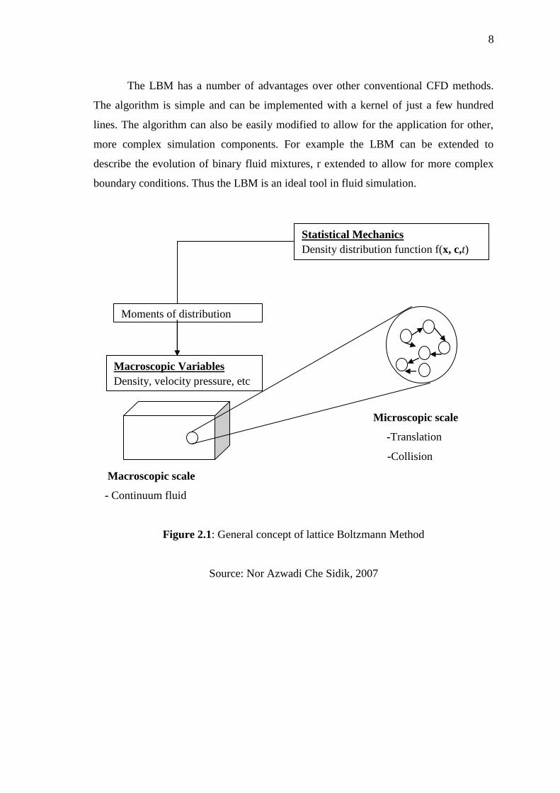
The LBM has a number of advantages over other conventional CFD methods.

The algorithm is simple and can be implemented with a kernel of just a few hundred

lines. The algorithm can also be easily modified to allow for the application for other,

more complex simulation components. For example the LBM can be extended to

describe the evolution of binary fluid mixtures, r extended to allow for more complex

boundary conditions. Thus the LBM is an ideal tool in fluid simulation.

Microscopic scale

-Translation

-Collision

Macroscopic scale

- Continuum fluid

Figure 2.1: General concept of lattice Boltzmann Method

Source: Nor Azwadi Che Sidik, 2007

Statistical Mechanics

Density distribution function f(x, c,t)

Moments of distribution

function

Macroscopic Variables

Density, velocity pressure, etc

9

2.3 Kinetic Theory

Consider a dilute gas consisting of hard spherical particles moving at great

velocity (~300 𝑚𝑠−1). We limit their interaction to elastic collisions. Hypothetically, it

would be possible to know the position vector (𝑥) and momentum (𝒑) of each

individual particle at some instant in time. Such information would give the exact

dynamical state of the system which, together with classical mechanics, would allow

exact prediction of all future states. We could describe the system by a distribution

function

𝑓(𝑁)(𝒙(𝑁), 𝒑(𝑁), 𝑡) (2.1)

where N is the number of particles. Here the distribution is thought of as residing in a

‘phase space’, which is a space in which the coordinates are given by the position and

momentum vectors and the time. Changes in Eq.(2.1) with time are given by the

Liouville equation (6N variables). However, this level of description is not possible for

real gases, where ~1023 (a mole of) particles are involved in just 20 liters of gas at

atmospheric temperature and pressure. Fortunately we are usually interested only in low

order distribution functions (N = 1, 2)(Orszag SA, 1995).

2.4 First Order Distribution Function

Statistical Mechanics offers a statistical approach in which we represent asystem

by an ensemble of many copies. The distribution

𝑓(1)(𝒙, 𝒑, 𝑡) (2.2)

gives the probability of finding a particular molecule with a given position and

momentum; the positions and moments of the remaining N-1 molecules can remain

unspecified because no experiment can distinguish between molecules, so the choice of

which molecule does not matter.

10

This is the ‘Single particle’ distribution function. 𝑓(1) is adequate for describing

all gas properties that do not depend on relative positions of molecules (dilute gas with

long mean free path).

The probable number of molecules with position coordinates in the range x ± dx

and momentum coordinates 𝒑 ± 𝑑𝒑 is given by

𝑓(1)(𝒙, 𝒑, 𝑡)𝑑𝒙𝑑𝒑 (2.3)

It introduce an external force 𝑭 that is small relative to intermolecular forces. If there

are no collisions, then at time t + dt, the new positions of molecules starting at 𝒙 are

𝒙 + (𝒑/𝑚)𝑑𝑡 = 𝒙 + (𝑑𝒙/𝑑𝑡)𝑑𝑡 = 𝒙 + 𝑑𝒙 (2.4)

and the new moments are

𝒑 = 𝒑 + 𝑭𝑑𝑡 = 𝑝 + (𝑑𝒑/𝑑𝑡)𝑑𝑡 = 𝒑 + 𝑑𝒑. (2.5)

Thus, when the positions and momenta are known at a particular time 𝑡, Incrementing

them allows us to determine 𝑓(1) at a future time 𝑡 + 𝑑𝑡:

𝑓(1)(𝒙 + 𝑑𝒙, 𝒑 + 𝑑𝒑, 𝑡 + 𝑑𝑡) 𝑑𝒙𝑑𝒑 = 𝑓(1)(𝒙, 𝒑, 𝑡)𝑑𝒙𝑑𝒑 (2.6)

This is the streaming process.

There are however collisions that result in some phase points starting at (𝒙, 𝒑)

not arriving at

(𝒙 + 𝒑/𝑚 𝑑𝑡, 𝒑 + 𝑭 𝑑𝑡) = (𝒙 + 𝑑𝒙, 𝒑 + 𝑑𝒑) (2.7)

and some not starting at (𝒙, 𝒑) arriving there too. We set Г(−)𝑑𝒙𝑑𝒑𝑑𝑡 equal to the

number of molecules that do not arrive in the expected portion of phase space due to

Documents

WAN MOHAMAD DASUQI BIN WAN MA’SOR - Welcome to …umpir.ump.edu.my/1914/1/Wan_Mohamad_Dasuqi_Wan_Ma'sor_(_CD_4943_).pdf · WAN MOHAMAD DASUQI BIN WAN MA’SOR Report submitted in