W. M. Keck Institute for Space Studies Postdoctoral ...kiss.caltech.edu/papers/reports/nicolas-lee-final-report.pdf · Postdoctoral Fellowship Final Report Nicolas Lee ... (2014),

W. M. Keck Institute for Space Studies

Postdoctoral Fellowship Final Report

Nicolas Lee

April 2013 – September 2015

Introduction

The W. M. Keck Institute for Space Studies (KISS) postdoctoral fellowship provided a

unique opportunity to pursue my research goals and participate in a wide range of projects. The

environment at Caltech and its proximity to JPL fosters a high degree of collaboration, leading to

partnerships with other research groups and exposure to their expertise. Additionally, the KISS

community played a major role through the availability of workshops, short courses, seminars,

and panels on a variety of interesting topics. These events allowed the graduate student and

postdoctoral fellows to interact with each other and with many distinguished scientists and

engineers.

Research Summary

During my postdoctoral appointment as a member of Professor Sergio Pellegrino’s Space

Structures Laboratory, my goal was to study enabling technologies for large deployable space

systems. To this end, my work focused on three main topics: deployable truss modules for

robotic assembly, packaging and deployment of ultra-light membrane structures, and high-

voltage low-power electronics design for small satellites.

In-space robotic assembly of modular trusses is a critical technology for the construction of

large, rigid space structures. An example of this is the International Space Station, whose

primary structure consists of ten truss components launched separately and assembled in low

Earth orbit. We collaborated with the Mobility and Robotic Systems section at JPL and with

Professor Joel Burdick’s research group at Caltech to develop an architecture and conceptual

design for a formation-flying, modular space telescope with a primary mirror backplane that is

constructed from lightweight hexagonal truss modules [Lee et al., in prep; Hogstrom et al., 2014

(attached)]. My contributions to this project included initial trade studies on truss module

geometry, prototype construction, and an assessment of space environment effects on the

performance of the telescope. Additionally, I developed a design algorithm to prescribe the

locations of hexagonal segments over a spherical surface, which is a non-trivial problem because

of the effect of variable gap width between segments [Lee et al., 2015 (attached)]. These gaps

have an impact on the optical performance of the telescope and on the geometry of the backplane

structure.

For space structures that are relatively flat, an attractive option for mass reduction is to

construct much of the surface using membranes that can be folded or rolled for efficient

packaging during launch. Applications include solar sails and drag sails, which require only a

thin membrane, as well as more complicated systems such as patch antenna arrays and solar

panels, which may incorporate rigid elements or multiple membrane layers. My work in this

area focused on membrane structures with integrated electronics, such as the design of a curved

crease pattern for packaging a two-layer membrane antenna array [Lee and Pellegrino, 2014a, b

(attached)], and structural concepts including antenna and photovoltaic elements for a space-

based solar power application [Arya et al., in prep.]. A key membrane-packaging concept we

explored is the use of a slipping fold that accommodates the thickness of the membrane. Our

collaborators for the space-based solar power project include Professors Harry Atwater and Ali

Hajimiri and their research groups at Caltech, as well as Northrop Grumman.

A continuing project in our research group is the Autonomous Assembly of a Reconfigurable

Space Telescope (AAReST) mission, which will fly several technology demonstrations on a

small satellite. A key technology for the reconfigurable space telescope is the use of thin

deformable mirrors whose shapes can be adjusted and controlled using an arrangement of

piezoelectric elements. My focus within this project was to design, build, and test high-voltage

electronic subsystems that drive the piezoelectric elements while satisfying the severe power and

volume constraints of the small satellite.

Acknowledgments

First and foremost, I wish to thank the W. M. Keck Institute for Space Studies, Michele Judd,

and Tom Prince for supporting my postdoctoral appointment, and Sergio Pellegrino, my

postdoctoral advisor, for his guidance. My time at Caltech would not have been as pleasant

without the community of KISS fellows and the students and postdocs of the Space Structures

Lab with whom I interacted on a daily basis. I would also like to thank the many colleagues at

Caltech and JPL who collaborated on projects and proposals, as well as all of the administrative

staff at KISS, the International Scholar Services, GALCIT, and EAS who make our work

possible.

Refereed Journal Articles

Lee, N. et al., Architecture for robotic in-space assembly of a modular space telescope,

Journal of Astronomical Telescopes, Instruments, and Systems (in preparation).

Arya, M., N. Lee, and S. Pellegrino, Packaging thick membranes with slipping folds for

crease-free compaction, AIAA Journal (in preparation).

Goel, A., N. Lee, and S. Close (2015), Estimation of hypervelocity impact parameters from

measurements of optical flash, Int. J. Impact Eng., 84, 54–63, doi:

10.1016/j.ijimpeng.2015.05.008.

Lee, N., S. Pellegrino, and Y.-H. Wu (2015), A design algorithm for the placement of

identical segments in a large spherical mirror, Journal of Astronomical Telescopes,

Instruments, and Systems, 1(2), 024002, doi:10.1117/1.JATIS.1.2.024002.

Close, S., I. Linscott, N. Lee, T. Johnson, D. Strauss, A. Goel, D. Lauben, R. Srama, A.

Mocker, and S. Bugiel (2013), Detection of electromagnetic pulses produced by

hypervelocity micro particle impact plasmas, Physics of Plasmas, 20, 092102, 1–8,

doi:10.1063/1.4819777.

Conference Papers

Arya, M., N. Lee, and S. Pellegrino (2016), Ultralight structures for space solar power

satellites, AIAA Space Structures Conference (in preparation).

Arya, M., N. Lee, and S. Pellegrino (2015), Wrapping thick membranes with slipping folds,

AIAA Space Structures Conference, Kissimmee, FL.

Hogstrom, K., P. Backes, J. Burdick, B. Kennedy, J. Kim, N. Lee, G. Malakhova, R.

Mukherjee, S. Pellegrino, Y.-H. Wu (2014), A robotically-assembled 100-meter space

telescope, Proc. IAC, Toronto, Canada.

Lee, N. and S. Pellegrino (2014), Packaging and deployment strategies for synthetic aperture

radar membrane antenna arrays, URSI-GASS, Beijing, China.

Tarantino, P., N. Lee, S. Close, and D. Lauben (2014), Faraday Plate Array analysis of

hypervelocity impact experiments, Spacecraft Charging and Technologies Conference,

Pasadena, CA.

Lee, N. and S. Pellegrino (2014), Multi-layered membrane structures with curved creases for

smooth packaging and deployment, AIAA Space Structures Conference, National Harbor,

Maryland.

Lee, N., S. Close, and R. Srama (2013), Composition of plasmas formed from debris impacts

on spacecraft surfaces, Sixth European Conference on Space Debris, Darmstadt,

Germany.

Talks and Posters

Impact plasma measurements using deployable CubeSat sensors, National Academies

Community Symposium on Achieving Science Goals with CubeSats, Irvine, CA,

September 2, 2015.

Asteroid surface resource characterization through plasma analysis of meteoroid impact

ejecta, Stanford Meteor Environment and Effects, Stanford, CA, July 16, 2015.

In-space robotic assembly of a modular telescope structure, Caltech Solid Mechanics

Symposium, Caltech, Pasadena, CA, February 13, 2015.

Membrane packaging techniques for space applications, KNI/MDL Seminar Series, Caltech,

Pasadena, CA, October 7, 2014.

Studying space rocks!, Summer Science Program, Socorro, NM, July 14, 2014.

Medicine, meteoroids, and membrane structures, GALCIT Colloquium, Pasadena, CA,

February 28, 2014.

65th International Astronautical Congress, Toronto, Canada. Copyright ©2014 by the International Astronautical Federation. All rights reserved.

IAC-14-C2.2.6 Page 1 of 12

IAC-14-C2.2.6

A ROBOTICALLY-ASSEMBLED 100-METER SPACE TELESCOPE

Main Author

Ms. Kristina Hogstrom

California Institute of Technology, United States, [email protected]

Co-Authors

Dr. Paul Backes

Caltech/JPL, United States, [email protected]

Prof. Joel Burdick


Mr. Brett Kennedy

Jet Propulsion Laboratory, United States, [email protected]

Dr. Junggon Kim


Dr. Nicolas Lee


Ms. Galina Malakhova


Dr. Rudranarayan Mukherjee


Prof. Sergio Pellegrino

Caltech/JPL, United States, [email protected]

Mr. Yen-Hung Wu


The future of astronomy may rely on extremely large space telescopes in order to image Earth-sized exoplanets or

study the first stars. In-Space Telescope Assembly Robotics (ISTAR) is a new paradigm for developing large

telescopes while overcoming some of the most limiting constraints of current designs. The ISTAR project has

developed a concept for an optical space telescope with a collecting area of nearly 8000 m2, launched in pieces from

the ground, and assembled by a dexterous robot in space. The proposed concept breaks the cost curve by using unique

optical layouts, a high degree of modularity, bulk manufactured parts, lightweight structures, and formation flying.

Preliminary analysis shows that the design meets high-level optical requirements to yield diffraction-limited images

with a wavefront correction system.

This paper focuses on the concept and structural analysis of the telescope. Presented first is the optical scheme,

which utilizes a spherical mirror 131 m vertex-to-vertex. Structural requirements are then derived from the limitations

of the wavefront control system. The remainder of the paper details the concept of the primary mirror, the largest and

most complex component, consisting of two layers: mirror segments and a supporting truss structure. Because the

mirror is spherical, every mirror segment is identical, which facilitates a highly modular structure. The 6289 segments

in the mirror layer are grouped into 331 mirror modules, each containing 19 segments and all associated actuators.

Each mirror module is backed by a deployable truss module. The robot builds the mirror by deploying and connecting

all truss modules first, then crawling on the resulting stiff surface to place each mirror module. The truss module

provides stiffness and support to the mirror, and thus it must be designed to meet and maintain precision requirements

under operational loads. The effect of the following loads on the structure are analyzed: fabrication and assembly

errors, gravity gradients, thermal effects, and vibrations. A concept of the truss module that meets requirements is

derived and presented.

I. INTRODUCTION

The bigger the telescope, the deeper we can probe, the

fainter we can detect, the wider we can survey, and thus

the better we can understand the universe. In 2018, the

James Webb Space Telescope (JWST) is scheduled to

become the largest ever built, and concepts for its even

bigger successor are already being formulated1. At just

6.5 m in aperture diameter, JWST is already too large to

fit in a payload fairing in its final configuration, and must

instead be assembled on Earth, folded for launch, and

unfolded in space. The most innovative foldable

concepts, like DARPA’s MOIRE and NASA’s

mailto:[email protected]




IAC-14-C2.2.6 Page 2 of 12

ATLAST, are sized at the 20 m range2, 3. The achievable

size of deployable telescopes is then strictly limited by

the size of the payload fairing. While advances in

lightweight and flexible materials can push this limit,

folding up and deploying a telescope many times larger

may not be realistic. The progression of space telescopes

thus necessitates a new strategy.

One solution is In-Space Telescope Assembly

Robotics (ISTAR). To reach larger scales, the telescope

can be assembled in space, rather than on the ground, no

longer limiting the aperture size by launch capacity. The

ISTAR concept presented here outlines an architecture

for a robotically-assembled optical space telescope that

can reach up to the 100-m class. The architecture is

entirely modular, enabling an expandable and evolvable

system that can be suited to meet a range of missions and

aperture sizes. This paper is focused on the development

and feasibility of the 100-m class telescope to stretch the

limits of the architecture. The complexity of constructing

a large aperture is addressed through symmetry and

modularity in the structure and use of robotic assembly.

The concept is based on a set of precision requirements

and correction methods using currently available

technology. In this paper, the concept of the primary

mirror, the largest component of the system, is described

in detail, including component design and assembly plan.

Preliminary structural and thermal analyses demonstrate

that the precision requirements can be met.

II. TELESCOPE CONCEPT

II.I Observatory Components

The ISTAR concept is a segmented, steerable, UV to

near IR telescope robotically assembled in space. Fig. 1

shows the basic layout of the telescope and its four main

components: the sunshade, primary mirror, Spherical

Aberration Corrector (SAC) unit, and metrology system.

Given the large size of the telescope, each of these

components is structurally separate and formation flown.

Each component is a self-contained unit with its own

power, thermal control, and propulsion system that

maintains formation.

The optical design borrows from that of the ground-

based Hobby-Eberly Telescope (HET) and Southern

African Large Telescope (SALT) by utilizing a spherical

curvature primary mirror4, 5. The primary mirror acts as a

“precision light bucket”, and is phased into a diffraction-

limited telescope at the exit pupil inside the SAC using a

technique described in Reference 6. One key advantage

of this design is that the majority of the wavefront sensing

and control (WFSC) and the only active deformable

mirrors are offloaded from the primary mirror to the

much smaller optics in the SAC. The primary mirror

segments are identical, manufactured in bulk, and only

require tip-tilt control, sharply reducing mirror

fabrication costs, which is one of the most significant cost

drivers in observatories. The SAC mirror segments have

the same basic characteristics, but are deformable with �m-level actuation range and correctable down to nm-

level. The baseline mirror segments are drawn from

currently available technology, and are assumed to have

a hexagonal shape with vertex-to-vertex length of 1.35

m. Because the segments are hexagonal, the full primary

mirror will also be approximately hexagonal. The

primary mirror parameters are summarized in Table 1.

The light-collecting area is equal to that of a 97.3-m filled

circular aperture.

Vertex-to-vertex length [m] 131.88

Light collecting area [m2] 7444

Radius of curvature [m] 800

Number of segments 6289

Segment vertex-to-vertex length [m] 1.35

Total areal density [kg/m2] < 30

Field of view [arc minutes] 4.2x4.2

Table 1: Primary mirror (M1) parameters.

Structurally connected to the primary mirror is also

the driving spacecraft and two solar panels similar to the

ones used on the International Space Station, as

determined by a preliminary power budget. The solar

panels are connected to the spacecraft, which is located

below the primary mirror in the center. The fully

assembled unit is shown in Fig. 2.

Fig. 2: Fully assembled primary mirror with central

spacecraft and solar panels. Fig. 1: Diagram of ISTAR optical scheme.


IAC-14-C2.2.6 Page 3 of 12

The SAC is located halfway to the center of curvature

of the primary mirror, for a separation distance of 400 m.

It includes two 8.6-m clamshell aspheric mirrors,

separated by 24.4 m. A ray trace diagram is shown in Fig.

4. Another major advantage of the spherical aperture is

that the SAC can be moved relative to the primary mirror

to observe a new target within a 7.16 deg field of regard

without having to move the massive primary mirror. This

enables rapid transition to a new observation without the

overhead of time and fuel otherwise required to slew the

primary mirror and wait for its dynamics to settle. The

locus of motion of the SAC with respect to the primary

mirror is a spherical surface of 400-m radius of curvature

and 50-m diameter, as shown in Fig. 5. In the nominal

position, the SAC is at the center and the entire primary

mirror is visible. However, when it is moved to the limit

of its range of motion, only about 40% of the primary can

be seen, as shown in Fig. 3.

The metrology system is located at the center of

curvature of the mirror. It contains a Zernike wavefront

sensor and an Array Hetroydyne Interferometer to

precisely measure the shape and phase of the primary

mirror segments.

The sun shade design borrows from deployable solar

sails such as Sunjammer, which is 38 m square and is

scheduled to be launched in 20157. Four deployable

masts extend from a central hub radially outward,

carrying the corners of the sun shade to a full distance of

70 m, as shown in Fig. 6. The Shuttle Radar Topology

Mission, launched in 2000, used a 60-m mast built by

ATK8. Thus, 70 m appears feasible with current

technology. The shade membrane will be chosen based

on thermal constraints described in Section IV.III.

II.II Primary Mirror Assembly Plan

The primary mirror is the largest component of the

telescope and thus the focus of robotic assembly. A

representation of the ISTAR robot needed to assemble

the mirror is shown in Fig. 8. The robot will be

commanded from Earth, but with significant on-board

autonomy to minimize the bandwidth of communications

to a human operator. The resulting supervised autonomy

system will enable the Earth-based operator to specify

high-level commands, while the robot performs all

sensor-based motion and complex tasks autonomously.

Drawing upon the development of the Lemur and

RoboSimian robots at JPL, the ISTAR robot is

anticipated to have six appendages 9, 10. During assembly,

two of these appendages can be used for dexterous

manipulation while the other appendages remain attached

to the structure. All six appendages can be used to walk

on the structure. Perception and dexterous manipulation

Fig. 5: Sketch highlighting the eyepiece motion

required to point to a new target without slewing the

primary mirror.

Fig. 3: Diagram of what portion of the primary mirror the

eyepiece sees when it is at the center (top) and 3.5 deg

from center. A side view of the telescope is shown left

and a top view is shown right.

Fig. 4: Ray trace diagram of the SAC.

Fig. 6: Model of the sun shade.


IAC-14-C2.2.6 Page 4 of 12

technologies that will be needed have been demonstrated

in a laboratory environment at JPL11. The robot is battery

powered and can be charged from the primary mirror

power grid.

The primary mirror consists of two layers: the mirror

segments, which includes rigid body actuators and

electronics, and a supporting truss structure. Because the

primary mirror is spherical, all mirror segments are

identical, which enables a highly modular structure.

Groups of segments and their actuators are hexagonally

packed into a cluster called a mirror module. Each mirror

module is backed by a rigid plate which features

structural and power connectors. Given the complexity

and fragility of the segments and associated electronics,

mirror modules are assembled on the ground by humans

and launched as a package.

The truss layer is broken down into hexagonal truss

modules, which are deployable structures sized to match

one mirror module when fully deployed but can stow

compactly for launch using internal hinges. An

assembled mirror module and truss module are shown in

Fig. 9. Each truss module is equipped with structural and

power connectors located at the ends of each vertical

member, with internal wiring throughout the members to

transmit power. These connectors are structurally

adjustable by the robot to ensure proper alignment

between modules. The vertices of the main face of each

module also features ball-like features which the robot

can grasp while walking.

In space, the robot retrieves the first folded truss

module from a central canister and deploys it so that the

internal hinges lock. The robot then attaches the truss

module at the connection points to a central hub that is

rigidly mounted and wired to the spacecraft and solar

panels. The robot then continues to assemble truss

modules in concentric rings around the central hub. After

each ring is assembled, a metrological measurement is

made to check the assembly for adherence to alignment

tolerances. The robot then uses this measurement to

adjust the connectors and complete the ring. This pattern

is repeated until the entire truss is built.

Once the truss is complete, the robot begins

assembling mirror modules. The robot interfaces with the

mirror module through the rigid plate, avoiding the

sensitive mirror segments. In the same concentric ring

pattern, the robot assembles mirror modules by attaching

them to the underlying truss. Mirror modules are

connected only to the truss, not to each other, to avoid

Fig. 8: Depiction of robot deploying a truss module.

Fig. 9: Mirror module atop truss module.

Fig. 7: Assembly concept showing how the truss modules

and mirror modules are stowed for launch and

assembled robotically in space.


IAC-14-C2.2.6 Page 5 of 12

stress build-up. The module assembly process is

summarized in Fig. 7.

It is unlikely that truss modules will need to be

serviced. However, mirror segments are sensitive and

may encounter issues (e.g. meteoroid hits). Servicing of

individual segments may be too complex for the robot, so

instead the entire mirror module can be replaced. The

connectors that attach the module to the truss will also be

able to detach from the truss as needed.

II.III Mission Requirements

The wavefront sensing and control system has three

levels of correction. First, as mentioned in the assembly

concept, the truss will be robotically adjustable during

construction. This corrects for fabrication and assembly

errors. Second, the primary mirror segments are backed

by rigid body actuators for removing quasistatic errors

such as thermal loads. Finally, the active mirrors in the

SAC remove any additional effects, including dynamic

errors. The correction levels, defined below, are

consistent with the current state-of-the-art.

Robotic truss adjustment: 30 mm to 3 mm

Rigid body actuators: 10 mm to �m -level

Active mirrors: �m -level to nm-level

o Also corrects up to 240 mm of change in

radius of curvature

The telescope design must ensure that errors remain

within the range of correction.

Along with the precision requirements, the following

other functional requirements must be met:

The telescope shall be functional no more than three

minutes after a slew maneuver.

The telescope shall operate at temperatures between

240 K and 300 K.

The primary mirror shall have an areal density less

than kg/m2. Since the mirror segments and

actuators have a density of 5 kg/m2, this leaves 5 kg/m2 for the truss.

Mirror segments shall have a gap of ± mm

to facilitate the ball-like features that the robot uses

to walk on the mirror surface.

The telescope shall nominally operate in a

geosynchronous orbit (GEO).

The ISTAR baseline to operate at GEO was chosen with

the expectation the telescope would then also be suited

for Lagrange point operation with few modifications,

because the environment at GEO is more severe and thus

produces more stringent design requirements.

The most customized parts of the architecture are the

truss and mirror modules. Their design, described in the

remainder of the paper, is based on these requirements.

III. MIRROR MODULE DESIGN

The mirror modules are all identical. Their geometry

is based on the following key considerations:

The module contains � identical, spherical mirror

segments arranged according to a hexagonal

tessellation.

The value of � is chosen to be as large as possible to

maximize launch capacity so that the modules can be

stacked inside a payload fairing.

The gaps between the mirror segments are ± mm to facilitate robotic mobility, as stated in

Section II.III.

The gap size between segments must vary to allow

the hexagonal segments to lie on a spherical surface.

Fig. 10 shows three choices for �: 7, 19, and 37 segments.

With the nominal 100-mm gap between segments, these

designs yield maximum mirror module dimensions of

3.77 m, 6.28 m, and 8.81 m respectively. Since the

proposed SLS launch vehicle will have a payload fairing

with an outer diameter of 8.4 m, the � = 9 design was

chosen12. With 6289 segments total, this design yields

331 mirror modules. Given their 25 kg/m2 areal density,

the total mass of the mirrors and actuators is then 145,300

kg.

The curvature of the mirror requires variable gap

sizes between the mirror segments. The distribution of

the gap size is a design parameter that has been studied

in detail. An algorithm to place the segments on a

spherical surface while imposing different constraints on

the gap variations was developed13. A solution was

obtained in which the gap sizes between mirror segments

within a mirror module vary by no more than 1.7 �m,

with the distribution being identical for all mirror

modules. The gaps between one mirror module and

another mirror module were also minimized with this

solution, with values ranging from 98 mm to 101.3 mm.

This result is well within the required tolerance of ± mm.

The mirror modules will be assembled on the ground,

incorporating the variable gap distribution that has been

calculated. The variation in the larger gaps between

Fig. 10: Choices of number of mirror segments per mirror

module.


IAC-14-C2.2.6 Page 6 of 12

modules will be created by the robot using the adjustable

connectors on the truss modules described in Section

II.II. Note that the gaps between the modules increase

linearly with depth through the truss thickness, and hence

will be larger on the back side of the truss than on the

front. However, because the radius of curvature is much

larger than the depth of the truss, the difference is still

well within the range of the adjustable connectors.

IV. TRUSS MODULE DESIGN

The truss geometry must facilitate a compact storage

profile and a smooth deployment. A modified version of

the Pactruss deployment scheme has been selected.

Pactruss was developed by Aerospace Corporation

specifically for large precision telescope structures14. It

was originally intended to provide an entirely deployable

telescope backing structure, consisting of many

triangular unit cells simultaneously unfolding. One flavor

of the deployment scheme is shown in Fig. 11. This

design was analyzed to show that it could maintain sub-

micron precision under operational loads when fully

deployed. However, there were issues in the deployment

simulations controlling the order in which the many

hinges were locked14. The ISTAR concept removes this

uncertainty because only one hexagonal unit cell is

required for the truss module, greatly reducing the

number of hinges that act simultaneously. The module

and deployment scheme are shown in Fig. 12. The unit

cell consists of 39 members: the 12 longerons that make

the hexagonal face on each side (24 total), 7 verticals, 4

face diagonals, and 4 internal diagonals. The diagonals

and 8 longerons are hinged in the center. In the compact

state, the truss module folds like an umbrella, and thus

the stowage footprint is determined by the hinge offsets

and the outer diameter of the members.

The truss module dimensions are defined in Fig. 13.

In order to reduce the number of redundant members, the

truss modules are rotated with respect to the mirror

modules, rather than hexagonally packed, as shown in

Fig. 14. The value of the side length � must match this

tesellation pattern, governed by the mirror module size.

For � = 9 as chosen, � = .6 m.

M55J carbon fiber composite has been selected for

the truss material, because of its high stiffness and low

density15. The truss depth, �, and member cross-section

properties, �� and �, control the structural response to

external loads, and thus must be chosen to ensure that all

of the precision requirements for the primary mirror are

met.

It is not known which source of shape error is in

general the most demanding for a large space telescope.

Thus, to determine the specific values of the design

variables of the truss module, it is necessary to consider

Fig. 11: Deployment of 20-meter hybrid Pactruss,

deploying around a central hub14.

Fig. 12: Truss module deployment.

Fig. 13: Geometry variables of truss module, with the

member cross-section shown right.

Fig. 14: Depiction of mirror module tiling (green outline)

vs. truss module tiling (purple outline).


IAC-14-C2.2.6 Page 7 of 12

separately the requirements associated with each specific

error source.

IV.I Fabrication and Assembly Errors

The fabrication and assembly errors must not exceed

30 mm (see Section II.III). The accuracy with which the

truss can be built is currently unknown, as the joints,

hinges, and connectors in the truss have yet to be

designed, and the manipulation capabilities of the robot

are not known in detail. Hence, assembly errors on the

level of 10 mm, 1 mm, and 0.1 mm were considered to

estimate the accuracy level needed to meet the 30 mm

precision requirement. These errors were treated as

length changes, ��, in the members of the truss to

represent fabrication errors or slide in the hinges. A pin-

jointed model of the truss was built in MATLAB. Each

member was assigned a �� value from a random uniform

distribution with maximum amplitude given by the

accuracy level. The resulting displacements were

computed and this process was repeated 10 times for each

accuracy level to obtain average and maximum values.

IV.II Gravity Gradient

Gravity gradients arise when one part of the telescope

is closer to the Earth than another part. This effect is

negligible for small telescopes, but becomes more

significant for larger Earth-orbiting telescopes. Gravity

gradients cause quasi-static errors in the mirror figure,

and thus the resulting distortion magnitude cannot exceed

10 mm, as discussed in Section II.III.

The magnitude of the gravity gradient distortion on

the primary mirror depends on its orientation with respect

to the Earth. The maximum gravity gradient occurs when

the mirror is oriented radially along the line of gravity, as

shown left in Fig. 15, causing an axial distortion.

However, the truss is much stiffer axially than in

bending, and thus other orientations that have less of a

gravity gradient may still have greater distortion.

In general, the distorting force on any node within the

primary mirror comes from the difference between the

gravitational force and the centrifugal force, which is set

by the orbit. If the vector between the center of mass of

the mirror and the center of the Earth is �, then the

centrifugal force, ��, on a node � of mass �� is given by:

�� = ��||�|| [1]

Letting �� be the vector between the center of mass and

the node �, the gravitational force, ��, is given by:

�� = �� − ��||� − ��|| [2] �� is then the difference between these forces.

The distortions due to gravity gradient loads were

computed from a finite element model of the primary

mirror structure, consisting of pin-jointed elements and

lumped masses distributed throughout the top surface to

represent the mass of the mirrors and actuators. The

nodes associated with the center module were fixed. The

mass matrix for the entire model was computed and the

mass associated with each node was used to calculate the

gravity gradient loads. The depth and member cross-

section were varied until an acceptable solution was

found.

IV.III Thermal Analysis

The bulk thermal requirement is that the primary

mirror must operate at 7 ± K, as stated in Section

II.III. However, one of the most detrimental thermal

effects is a change in curvature of the primary mirror,

which arises from a temperature difference through the

mirror thickness, or from the mirror surface to the

backside of the truss. The rigid body actuators, with a

range of 10 mm, can correct for this type of error. In

addition, the wavefront control in the eyepiece can

counteract 240 mm of additional change in the radius of

curvature from the nominal 800 m.

When the curvature changes, the sag of the mirror

changes. The sag � is the height difference between the

mirror edge and mirror center, as shown in Fig. 16. The

aperture diameter � is defined in this picture as an

arclength on the circle of radius R that subtends angle �.

This is to ensure that, as � changes, the length of the

mirror neutral axis stays constant. If � is small (only

about .5 ° in the nominal case), the sag � is

approximately �⁄ / � . The rigid body actuators

can account for change in sag �� of 10 mm. Given that

the average diameter of the hexagon is about � = m,

Fig. 16: Definition of the sag value x. D is the arclength

defined by angle ϕ on the circle of radius R.

Fig. 15: Orientation of the primary mirror with maximum

gravity gradient (left), intermediate gravity gradient

(middle), and minimum gravity gradient (right).


IAC-14-C2.2.6 Page 8 of 12

the maximum change in curvature Δ� that can be

removed by the rigid body actuators is given by:

Δ� = Δ �⁄ = ��= . × − m−

[3]

The wavefront correction system can account for an

additional curvature change of Δ� = Δ �⁄ = / m − / . m = . × − m− . Thus the

total allowable curvature change is Δ�� = . ×− m− . The curvature is then related to the temperature

differential by the truss depth � and material expansion

coefficient ��:

Δ�� = �� [4]

Given �� = . × − /°C for M55J carbon fiber

composite and the curvature change obtained above,

Equation [4] yields the maximum allowable temperature

difference in terms of the truss depth, Δ�� = . ∙� [°C]. In GEO, there are three distinct thermal

environments, shown in Fig. 18. The temperature

gradient in each case was estimated using energy balance

on a simple thermal model. Fig. 17 shows a module of

the model, where surface 1 is the mirror surface and

surface 2 is the back surface of the truss, consisting of a

triangular tessellation of members with large gaps in

between them.

In case 1, the telescope is pointed at the Earth with the

Sun behind the sun shade. Surface 2 receives heat from

the Sun that leaks through the sun shade. Surface 1

receives heat from the Earth’s surface radiation and

albedo reflection from the Sun, as well as heat from the

Sun that leaks through the sun shade and is not blocked

by Surface 2. In addition, both surfaces exchange heat

through radiation and conduction. By defining each of

these inputs, the temperatures of both surfaces were

found from the energy balance. The geometric

parameters of the truss, the optical properties of the

materials, and the fraction of heat blocked by the sun

shade were varied until the temperatures were within ± K and the difference between the temperatures

was less than the requirement. The full energy balance

derivation can be found in Appendix A.

IV.IV Dynamics

It is assumed that, in order to passively reject

vibrations and maintain the required dynamic precision

of 1 �m, the fundamental frequency must be higher than

the frequency of vibrations. One of the major sources of

vibrations are reaction wheels. From Reference 16, the

requirement on the fundamental frequency of the

structure to reject reaction wheel disturbances is given

by:

� > {��√�� − , �� ≥�� , �� < �� = ��

[5]

where � is the telescope fundamental frequency, �� is the

cut-off frequency of the isolation system, �� is the

number of reaction wheels, �� is the static reaction wheel

imbalance, � is the damping coefficient, �� is the

total mass of the telescope and spacecraft, and �� is

the maximum allowable deformation.

In the present case, �� =1 �m, and the damping

coefficient was conservatively chosen as 0.005.

Reference 16 states that a typical value for �� is ×− kg ∙ m. It can be assumed that �� < , and the

fundamental frequency of the structure only needs to

exceed the isolation cut-off frequency in order to

maintain precision under reaction wheel imbalance loads.

Isolation systems can achieve cut-off frequencies on the

order of 0.1 Hz17.

Fig. 17: Thermal model of one module of primary

mirror.

Fig. 18: GEO thermal environment cases. Case 3

represents the eclipse condition.


IAC-14-C2.2.6 Page 9 of 12

There are many other possible sources of vibrations

on the spacecraft, such as the mirror actuators and joint

settling. Control moment gyros may also be used instead

of reaction wheels, which will have different vibration

characteristics. Rather than addressing each source

individually, it is practical to assume a spectrum of

random vibrations. The minimum fundamental

frequency to reject random disturbances is given by:

� > � ( ��) [6]

where � is the RMS amplitude of the disturbance power

spectral density over the bandwidth of their

frequencies17. Assuming a �� amplitude and a 0-100 Hz

bandwidth, � = . × −6 m s⁄ Hz⁄ = . ×− m s⁄ , which yields a minimum fundamental

frequency of the telescope of 0.459 Hz.

Finally, one functional requirement is that the

telescope shall be usable no more than three minutes after

a slew maneuver. The exact response of the structure to a

slew maneuver depends on the torque profile, the

propulsion system, and other parameters not specified at

this design stage. However, the settling time �� required

for structural distortions to fall below 2% of the initial

distortion amplitude can be estimated by considering a

single-degree-of-freedom system: �� = . /�� , where � = �� . Again assuming � = . and requiring

that �� < minutes implies that the fundamental

frequency must be larger than 0.69 Hz, which is the most

stringent dynamic requirement.

The fundamental frequency was estimated from the

finite element model described in Section IV.II.

IV.V Analysis Results

After an iterative process that included each of the

loading types outlined above, the design converged to the

parameters presented in Table 2.

Truss side length, � [m] 2.6

Truss depth, � [m] 2.6

Member outer diameter, �� [mm] 45

Member wall thickness, � [mm] 3

Truss areal density [kg/m ] 4.01

Truss mass [kg] 23352

Primary mirror mass [kg] 168690

Table 2: Truss module design parameters

Firstly, as described in Section II.III, the truss areal

density is confined to less than kg/m . This

requirement is met with a margin of kg/m , which may

be allotted to the mass of the truss hinges and connectors.

This design has a fundamental frequency of 1.0 Hz,

which satisfies the dynamic requirements with a good

margin. Despite the size of the telescope, the effect of

gravity gradient was still negligible. The maximum

distortion occurred when the mirror was oriented

approximately deg to the line of gravity (as roughly

shown middle in Fig. 15), but this distortion did not

exceed 46 nm.

Assembly errors on the level of 10 mm, 1 mm, and

0.1 mm were applied to the truss. The resulting

distortions of the truss were computed to obtain the RMS

and maximum distortion on the mirror surface in the

direction normal to the curvature, as well as the RMS and

maximum overall distortion, which are shown in Table 3.

The maximum distortions indicate that the input error can

be greatly amplified in the structure, in some cases by a

factor of almost six, demonstrating the effect of error

build-up. It follows that, in order to meet the maximum

30-mm requirement, the structure must be built to a

precision of at least 5 mm.

Error level 10 1 0.1

RMS Surface Distortion 92.51 0.91 0.12

Max Surface Distortion 55.70 1.56 0.69

RMS Total Distortion 9.73 0.96 0.12

Max Total Distortion 57.10 5.63 0.71

Table 3: Results of fabrication error analysis. The units

are all in millimeters.

From Equation [4], given � = . meters, the

maximum allowable temperature difference through the

truss thickness is Δ� = . K. The thermal analysis

was performed using the parameters given in Table 4,

where �� and �� are the absorptivity and emissivity of

surface � respectively, which can vary between the top

and bottom of the surface (refer to Fig. 17).

Solar flux �� [W/m ] 1370

Earth surface heat flux �� [W/m ] 237

Earth albedo � 0.3

Orbit altitude �� [m] 35786

Earth radius �� [m] 6378 � ,�� (Polished aluminum) 0.02 � ,�� (Paint) 0.6 � ,�� = � .�� (CFC) 0.96 � ,�� (Polished aluminum) 0.03 � ,�� (Paint) 0.87 � ,�� = � .�� (CFC) 0.88

CFC thermal conductivity � [W/m] 156

Fraction of solar flux blocked by shade � 0.6

Table 4: Parameters used in thermal analysis. CFC stands

for carbon fiber composite, assumed to be roughly

matte black.

Note that the bottom of the mirror modules is coated with

flat colored (red, green, or brown) paint to yield the

desired optical properties, while the truss maintains the


IAC-14-C2.2.6 Page 10 of 12

optical and thermal properties associated with black

carbon fiber composite. The resulting temperatures of �

and � for the three different environmental cases are

shown in Table 5.

� [K] � [K] Δ� [K] Case 1 278.03 273.29 4.74

Case 2 277.96 273.26 4.70

Case 3 89.21 86.59 2.62

Table 5: Thermal analysis results.

The bulk temperature constraint of 70 ± 0 K is

maintained in only two of the cases; the thermal analysis

shows that the telescope will not be able to operate when

it is eclipsed by the Earth. In GEO, eclipses only occur

during 3 months of the year, lasting 72 minutes at

maximum, so this is an acceptable mission constraint.

When not eclipsed, a modest sun shade blockage factor

of � = 0.6 keeps the primary mirror within temperature

bounds and with an acceptable gradient through the truss

thickness to maintain precision requirements. The

material of the sunshade will have to be chosen to obtain

this blockage factor.

V. SUMMARY

This paper has outlined a solution for 100-m optical

telescope that is robotically assembled. The concept

breaks the cost curve by utilizing an optical design with

a spherical primary mirror. The shape allows for the

wavefront sensing and control system to be offloaded to

an eyepiece, so that the primary mirror segments can be

inactive and identical, sharply reducing the cost of the

control system and mirror fabrication. The assembly

process of the primary mirror efficiently balances

deployable structures with robotic operations. The

primary mirror is broken down into groups of mirror

segments called mirror modules, backed by separate

deployable truss modules. In orbit, the robot deploys and

assembles the truss around a central hub connected to a

spacecraft, then attaches the mirror modules to the truss.

The mirror modules have been sized to fit in the proposed

SLS payload fairing. The truss modules provide stiffness

and support to the mirror surface. Preliminary structural

and thermal analyses have been performed to design the

truss module and demonstrate that it can provide

precision levels within the range of the wavefront

correction system to yield diffraction-limited images.

Some important parameters of the telescope are

summarized by Table 6.

The telescope presented here is currently in the

concept stage. Results so far are promising, and work is

ongoing to bring the concept to a higher level of maturity.

This includes better characterization of the metrology,

eyepiece, and sun shade, as well as continued

development of the structural components and robotic

assembly.

VI. ACKNOWLEDGEMENTS

The research was carried out in part at the Jet

Propulsion Laboratory, California Institute of

Technology, under a contract with the National

Aeronautics and Space Administration. Part of this work

was supported by the NASA Space Technology Research

Fellowship #NNX13AL67H.

Primary Mirror vertex-to-vertex (V2V)

length [m]

131.88

Light collecting area [m2] 7444

Radius of curvature [m] 800

Field of view [arc min] 4.2x4.2

Field of regard [deg] 17.6

SAC to primary mirror distance [m] 400

SAC largest mirror dimension [m] 8.6

SAC clamshell mirror separation [m] 24.4

Number of primary mirror segments 6289

Number of mirror modules 331

Number of truss modules 331

Number of concentric rings 10

Mirror segment V2V length [m] 1.35

Truss module V2V length [m] 5.2

Mirror module V2V length [m] 6.28

Mirror segment aerial density [kg/m2] 25

Truss aerial density [kg/m2] 4.01

Sunshade diagonal dimension [m] 140

Operating temperature [K] 240-300

Sunshade blockage factor 0.6

Truss module mass [kg] 70.54

Mirror module mass [kg] 439.0

Truss member outer diameter [mm] 45

Truss member wall thickness [mm] 3

Truss module depth [m] 2.6

Table 6: Important parameters of the ISTAR telescope

concept

APPENDIX A. THERMAL ENERGY BALANCE

The energy balance equations will be developed here

for case 1, since all factors are present. Equations for case

2 and 3 can be derived by removing and rearranging the

appropriate terms. In general, the balance for case 1 is as

shown in Equation [7].

Surface 1: �� + �� + � ,�� − ��, → − ��, →− � ,�� = 0

Surface 2: � ,�� + ��, → + ��, → − � ,�� = 0

[7]

�� ≔ heat from Earth internal radiation

incident upon surface 1 �� ≔ heat from Earth albedo reflection

incident upon surface 1 ��, → ≔ heat conducted from surface 1 to

surface 2


IAC-14-C2.2.6 Page 11 of 12

��, → ≔ heat radiated from surface 1 to

surface 2 � ,�� ≔ heat from Sun leaking through the

shade and incident upon surface 1 � ,�� ≔ heat from Sun leaking through the

shade and incident upon surface 2 � ,�� ≔ heat radiating from surface 1 to

space � ,�� ≔ heat radiating from surface 2 to

space

Note that heat leaking through the sun shade can be

incident upon surface 1 through the gaps between the

truss members.

Each surface � has area ��, with top and bottom

emissivity and absorptivity of ��,��, ��,��, ��,��, and ��,�� respectvely. The total area of the top surface � is

equal to the number of modules �� multiplied by the area

of one module with side length �. The area of surface 2

is only the projected area of the truss members arranged

in the triangular pattern shown left in Fig. 17. Each

Module has 12 surface members with outer diameter �

and length �. � and � are given by:

� = �� √ � � = ��

[8]

Given this geometry, the external heat fluxes are: �� = �� ,�� sin � �� = �� . + . �+ . � � � ,�� sin � � ,�� = − � �� − � � ,�� ,�� = − � �� ,�� ,�� = �(� ,�� + � ,��)�4 � ,�� = �(� ,�� + � ,��)�4

[9]

where �� amd �� are the surface heat flux from the

Earth and the heat flux from the Sun at 1 AU respectively,

and � is the fraction of solar heat that is blocked by the

sun shade18. The surface albedo of the Earth is � and sin � = ��/ �� + �� , where �� is the radius of

Earth and �� is the altitude of the orbit. The Stefan-

Boltzmann constant is � and � and � are the

temperatures of surfaces 1 and 2 respectively.

Conduction between the surfaces is carried through

the 7 verticals of length � and 8 diagonals of length √� + � in each module. The truss material has a

conductivity � and the cross-sectional area of the

members � is �/ � − �� , where �� is the inner

diameter. Thus the total conduction term is given by: ��, → = �� − � (�+ √� + � )

[10]

The last term to define is the radiation between the

two surfaces. Surface 2 can be treated as three arrays of

parallel cylinders separated by � = √ / �. The arrays

are oriented at ° angles to each other to comprise the

full triangular grid. It is assumed that the surfaces are

large enough with respect to the individual cylinders to

be treated as infinite. The view factor from an infinite

plate to an infinite array of parallel cylinders is shown in

Equation [11]19. � → = − [ − (�� ) ]+ �� tan− √� − ��

[11]

The total projected area of each array is �� , because

each module has four members of length � in each

direction. The total radiative heat transfer from surface 1

to the six arrays in surface 2 is then given by: ��, →= � �4 − �4− � ,�� ,�� + � � → + − � ,�� ,�� [12]

Substituting Equations [8]-[11] into Equation [7] yields

the full energy balance for the system, which can be

solved to obtain � and � . The temperature difference � − � must then be compared to that in Equation [4] to

ensure requirements are met.

REFERENCES

[1] "James Webb Space Telescope", NASA, Web:

http://www.jwst.nasa.gov/ (21 August 2014).

[2] M. Postman, T. Brown, K. Sembach, M. Giavalisco,

W. Traub, K. Stapelfeldt, D. Calzetti, W. Oegerle, R.

Michael Rich, H. Phillip Stahl, J. Tumlinson, M.

Mountain, R. Soummer, T. Hyde, Advanced

Technology Large-Aperture Space Telescope: science

drivers and technology developments, OPTICE, 51

(2012) 1-11.

[3] "MOIRE", Ball Aerospace and Technologies Corp.,

Web: http://www.ballaerospace.com/page.jsp?page=259

(21 August 2014).

[4] "Hobby-Everly Telescope", The University of Texas

- Austin, 2014, Web:

http://www.as.utexas.edu/mcdonald/het/het.html (21

August, 2014).

[5] "Southern African Large Telescope", Southern

African Astronomical Observatory, 2014, Web:

http://www.salt.ac.za/ (21 August 2014).

[6] A.B. Meinel, M.P. Meinel, Two-stage optics: high-

acuity performance from low-acuity optical systems,

OPTICE, 31 (1992) 11.

[7] "Sunjammer", 2014, Web:

http://www.sunjammermission.com/home (21 August

2014).

http://www.jwst.nasa.gov/

http://www.ballaerospace.com/page.jsp?page=259

http://www.as.utexas.edu/mcdonald/het/het.html

http://www.salt.ac.za/

http://www.sunjammermission.com/home


IAC-14-C2.2.6 Page 12 of 12

[8] "Articulated Mast Systems", Alliant Techsystems,

2014, Web: http://www.atk.com/products-

services/articulated-mast-systems (21 August 2014).

[9] "RoboSimian", Darpa Robotics Challenge, Web:

http://www.theroboticschallenge.org/teams/robosimian

(21 August 2014).

[10] B. Kennedy, H. Agazarian, Y. Cheng, M. Garrett,

G. Hickey, T. Huntsberger, L. Magnone, C. Mahoney,

A. Meyer, J. Knight, LEMUR: Legged Excursion

Mechanical Utility Rover, Autonomous Robots, 11

(2001) 201-205.

[11] N. Hudson, J. Ma, P. Hebert, A. Jain, M.

Bajracharya, T. Allen, R. Sharan, M. Horowitz, C. Kuo,

T. Howard, L. Matthies, P. Backes, J. Burdick, Model-

based autonomous system for performing dexterous,

human-level manipulation tasks, Autonomous Robots,

36 (2014) 31-49.

[12] "Space Launch System", NASA, Web:

http://www.nasa.gov/exploration/systems/sls/ (21

August 2014).

[13] N. Lee, S. Pellegrino, Y.-H. Wu, A design

algorithm for the placement of identical segments in a

large spherical mirror, 2014, (in preparation).

[14] J.M. Hedgepeth, Pactruss support structure for

precision segmented reflectors, National Aeronautics

and Space Administration, Langley Research Center,

Hampton, Va., 1989.

[15] "M55J Data Sheet", Torayca, Web:

http://www.toraycfa.com/pdfs/M55JDataSheet.pdf (21

August 2014).

[16] L. Peterson, G. Agnes, How the Mass of Large

Gossamer Optical Telescopes Scales with Size and

Disturbance Environment, 48th

AIAA/ASME/ASCE/AHS/ASC Structures, Structural

Dynamics, and Materials Conference, American

Institute of Aeronautics and Astronautics, 2007.

[17] W.K. Wilkie, R.B. Williams, G.S. Agnes, B.H.

Wilcox, Structural Feasibility Analysis of a Robotically

Assembled Very Large Aperture Optical Space

Telescope, 48th AIAA/ASME/ASCE/AHS/ASC

Structures, Structural Dynamics, and Materials

Conference, American Institute of Aeronautics and

Astronautics, 2007.

[18] M.D.G. Griffin, J.R. French, Space Vehicle

Design, American Institute of Aeronautics &

Astronautics, 2004.

[19] Y.A. Çengel, Heat and mass transfer : a practical

approach, McGraw-Hill, Boston, 2007.

http://www.atk.com/products-services/articulated-mast-systems

http://www.atk.com/products-services/articulated-mast-systems

http://www.theroboticschallenge.org/teams/robosimian

http://www.nasa.gov/exploration/systems/sls/

http://www.toraycfa.com/pdfs/M55JDataSheet.pdf

Design algorithm for the placement ofidentical segments in a large sphericalmirror

Nicolas LeeSergio PellegrinoYen-Hung Wu

Design algorithm for the placement of identicalsegments in a large spherical mirror

Nicolas Lee,a,* Sergio Pellegrino,a and Yen-Hung Wub

aCalifornia Institute of Technology, Graduate Aerospace Laboratories, 1200 East California Boulevard, Pasadena, California 91125, United StatesbCalifornia Institute of Technology, Jet Propulsion Laboratory, 4800 Oak Grove Drive, Pasadena, California 91109, United States

Abstract. We present a design algorithm to compute the positions of identical, hexagonal mirror segments on aspherical surface, which is shown to provide a small variation in gap width. A one-dimensional analog to thesegmentation problem is developed in order to motivate the desired configuration of the tiling patterns and toemphasize the desire for minimizing segment gap widths to improve optical performance. Our azimuthalequidistant centroid tiling algorithm is applied to three telescope architectures and produces mirror segmentarrangements that compare favorably with existing and alternative designs. © 2015 Society of Photo-Optical

Instrumentation Engineers (SPIE) [DOI: 10.1117/1.JATIS.1.2.024002]

Keywords: segmentation; space telescope; point spread function; Fourier optics.

Paper 14031 received Nov. 6, 2014; accepted for publication Feb. 3, 2015; published online Mar. 16, 2015.

1 Introduction

Since the invention of the telescope, astronomical observatories

have implemented increasingly larger apertures. More recently,

designs for both ground- and space-based astronomical tele-

scopes have included optical surfaces that exceed the manufac-

turing limits for a single monolithic mirror. These designs have

necessitated the development of segmented mirrors forming

a single large optical surface out of smaller elements. Typically,

these segmented mirrors use a hexagonal tiling pattern to

achieve a high fill factor. However, the curvature of the optical

surface prevents the hexagonal tiling from being perfectly uni-

form. As a result, telescope designs are forced to use mirror seg-

ments that are not identical in planform (the outlined shape of

the segment), or to accept nonuniform gaps between segments,

which increases the complexity of the mechanical design and

degrades signal-to-noise performance through increased diffrac-

tion effects.

The first telescopes to use a segmented primary mirror were

the Keck telescopes,1 completed in 1993 and 1996, followed by

the Hobby–Eberly Telescope (HET)2 and South African Large

Telescope.3 The James Webb Space Telescope (JWST) will be a

space-based segmented telescope with 18 segments.4 A concept

study for the next-generation space telescope is considering

three designs ranging from an 8 m monolithic mirror to a

16.8 m segmented primary with 36 segments.5 Table 1 summa-

rizes relevant parameters for these and other telescopes with seg-

mented mirrors, including both existing and proposed designs.

Most of these telescopes are designed with nonidentical segment

geometries. The Thirty Meter Telescope (TMT), for example,

uses six each of 82 unique mirror shapes to make up its 492

total segments.6 In order to accommodate maintenance and

occasional resurfacing to restore reflectivity, the telescope will

require the fabrication of seven of each segment type such that

each shape has one spare.

The aspherical surface figure of the primary mirror in these

telescopes requires the segment figures not to be identical. As a

result, there is little benefit to requiring identical planforms for

the segments. The design choice of using nonidentical segment

planforms allows these telescopes to implement a uniform gap

width between all segments. This maximizes the capture area of

the primary aperture, but becomes impractical for telescope

designs with too many segments to individually manufacture

and calibrate.

The use of unique segments becomes infeasible as the aper-

ture size continues to increase. For the proposed and eventually

canceled Overwhelmingly Large Telescope (OWL), the inclu-

sion of >3000 segments drove the design toward a spherical

primary mirror composed of identical segments.13 The similarly

sized In-Space Telescope Assembly Robotics (ISTAR) concept,

with >5000 segments, is a design for a robotically assembled

and serviceable space telescope.14 For such a design, segments

could be replaced in orbit when damaged, but not resurfaced.

Having a large number of uniquely shaped, spare segments in

this case would be extremely inefficient. Therefore, these large

telescope designs tend to use a spherical primary mirror with

mass-produced identical segments in both planform and figure.

However, in the future, advances in highly deformable, thin

mirrors could enable such identical mirror segments to achieve

an adequate optical figure even for an aspherical primary

design.15,16

This paper specifically addresses the problem of tiling iden-

tical hexagonal segments onto a spherical primary mirror. We

present a design algorithm to compute the positions of these seg-

ments on the spherical surface, which is shown to provide

a small variation in gap width. This design algorithm, which

we will refer to in this paper as the azimuthal equidistant cent-

roid tiling (AECT) algorithm based on the geometry developed

in Sec. 4, is not computationally intensive and can be applied to

a range of mirror geometries. We believe that it can be a valuable

*Address all correspondence to: Nicolas Lee, E-mail: [email protected] 2329-4124/2015/$25.00 © 2015 SPIE

Journal of Astronomical Telescopes, Instruments, and Systems 024002-1 Apr–Jun 2015 • Vol. 1(2)

Journal of Astronomical Telescopes, Instruments, and Systems 1(2), 024002 (Apr–Jun 2015)

http://dx.doi.org/10.1117/1.JATIS.1.2.024002








tool for rapid computation of optical configurations for early

design studies, without requiring the time or computational

power for an optimization-based technique. By focusing specifi-

cally on the problem of finding the ideal positions for mirror

segments, the AECT algorithm would complement an overall

system study that accounts for additional effects, including

but not limited to manufacturing and positioning error, secon-

dary optical elements, and active control systems.

In the following section, we provide an overview of the back-

ground and prior work on the design and analysis of the three-

dimensional geometries of highly segmented telescope mirrors.

Section 3 introduces a one-dimensional analog to the tiling

problem in order to provide insight into the effect of different

tiling options on the optical point spread function (PSF) using

Fourier optics. Section 4 presents the details of our new AECT

algorithm for tiling segments onto a spherical surface. Section 5

demonstrates that the proposed tiling strategy produces results

that are competitive with alternative methods. We show this by

applying the AECT algorithm to designs based on the HET,

OWL, and ISTAR concepts. Finally, Sec. 6 concludes and

summarizes.

2 Background

There has been much prior work on the design and analysis of

large segmented telescopes. In this section, we briefly highlight

some specific work that is relevant or complementary to the

problem of tiling identical segments on a sphere.

2.1 Telescope Design

The focus of this paper is on the effect of ideal positioning of

segments on a primary mirror. However, the overall performance

of a telescope is driven by many other factors. Many prior analy-

ses have considered complete optical systems rather than just the

primary mirror. For example, Jolissaint and Lavigne consider a

30 m design with adaptive optics,17 and Chanan et al. consider

active control of the mirror segments18 in a full telescope system.

The aberration introduced by a spherical primary mirror can

be corrected through additional optical elements, such as the

four-mirror, double Gregorian design used by HET.19

Additionally, operational techniques can be developed to

mitigate performance limitations. Large ground-based tele-

scopes are typically limited in angular resolution not by diffrac-

tion but by atmospheric distortion. This can be compensated by

adaptive optics or by postprocessing. Speckle imaging tech-

niques for postprocessing have been used to compensate for

this effect and to achieve higher angular resolution. For exam-

ple, the Keck telescope produced a 0.05 arc sec diffraction-

limited near-infrared image.20

The design of nominal mirror geometry in telescopes using

identical segments is not well documented in the literature.

Table 1 Hexagonally segmented telescope designs and relevant parameters.

Name Primary aperture dimension Number of segments Date constructed

Ground-based telescopes:

Keck 11 10 m 36 1985 to 1993

Keck 21 10 m 36 1991 to 1996

Hobby–Eberly Telescope (HET)2 11 × 10 m 91 1994–1997

South African Large Telescope (SALT)3 11 × 10 m 91 2000 to 2005

Large Sky Area Multiobject Fiber SpectroscopicTelescope (LAMOST)7

6.67 × 6.09 m 37 2001 to 2008

Gran Telescopio Canarias (GTC)8 10.4 m 36 2002 to 2008

Euro509 50 m 618 Merged with European ExtremelyLarge Telescope (E-ELT)

California Extremely Large Telescope (CELT)10 30 m 1080 Merged with Thirty MeterTelescope (TMT)

TMT6,11 30 m 492 2014 to 2022 (started)

E-ELT12 39.3 m 798 2014 to 2022 (started)

Overwhelmingly Large Telescope (OWL)13 100 m 3048 Canceled

Space-based telescopes:

James Webb Space Telescope (JWST)4 6.5 m 18 Expected 2018 launch

Advanced Technology Large-Aperture SpaceTelescope (ATLAST)5

8 to 16.8 m 1 or 36 Preliminary

In-Space Telescope Assembly Robotics (ISTAR)14 100 m >5000 Preliminary


Lee, Pellegrino, and Wu: Design algorithm for the placement of identical segments in a large spherical mirror

Published reports provide average segment gap width and

ranges of gap width variation for the HET and OWL designs,

but no details on the specific design algorithms used.2,13 The

design of the TMT primary mirror segmentation, which uses

variable mirror segments, was based on an optimization algo-

rithm that started with a planar hexagonal grid and introduced

a design variable that scales the tessellation as a function of dis-

tance from the optical axis to account for the mirror curvature.6

This grid was then cylindrically projected onto the mirror sur-

face to define the individual segment planforms.

2.2 Optical Analysis

Techniques for predicting and characterizing the optical perfor-

mance of a telescope can be partitioned into analytical and

numerical methods. Fourier methods are commonly used in

optical diffraction theory to compute the PSF of an aperture.21,22

Yaitskova et al. applied Fourier techniques to the study of large,

highly segmented telescope mirrors.23 The effects of errors from

segment position and misfigure are described, while the varia-

tion in gap width is reported as having little effect on the PSF.

One approximation for the proportion of energy Ep outside

the core PSF is

Ep ¼AF − AS

AF

; (1)

where AF is the surface area of the filled aperture and AS is the

total surface area of the segments not including the gaps.24 This

motivates the desire for a tightly packed arrangement of mirror

segments to achieve the best image quality.

Numerical methods include ray-tracing techniques to model

the optical behavior of a telescope and can be combined with

numerical models of the telescope environment, structure, and

other error sources to predict the overall system performance.25

3 One-Dimensional Segmentation Analog

As discussed in the previous section, the use of Fourier optics to

analytically determine the optical performance of a telescope

has been described extensively in the literature.21–23 It is well

known that segmentation of an optical aperture leads to a

speckle pattern in the PSF. Variation in the width of gaps

between mirror segments introduces intensity variations in

the PSF, which increase the background intensity while dimin-

ishing the peak intensity of the speckles. This effect does not

strongly influence the encircled energy of the PSF but does

have a substantial effect on the ratio between the intensities

of the central peak of the PSF and the nearest speckle peak.

Reducing the average gap width between segments is an effec-

tive method for improving the contrast performance of a seg-

mented telescope design by reducing the intensity of speckles

near the central peak.

For readers who are less familiar with the conclusions pre-

sented in the previous paragraph, we provide, in this section, the

following mathematical development demonstrating the effect

of mirror segmentation on a PSF. In particular, we wish to char-

acterize the effect of gap width variations between segments on

the PSF of the aperture. This provides a direct connection

between the geometry of the segments and a measure of the opti-

cal performance of the primary mirror. Considering Fraunhofer

diffraction, the PSF hðu; vÞ is computed from the two-dimen-

sional Fourier transform of the aperture function aðx; yÞ as

hðu; vÞ ¼ jF ½aðx; yÞ%j2: (2)

In a segmented mirror, the full aperture function aðx; yÞ canbe expressed as the convolution of the segment aperture sðx; yÞwith a grid factor gðx; yÞ, which is composed of an array of delta

functions. The PSF can, therefore, be decomposed as the prod-

uct of the individual Fourier transforms of the segment aperture

and the grid factor:

hðu; vÞ ¼ jF ½sðx; yÞ%F ½gðx; yÞ%j2: (3)

However, we find it worthwhile to consider first a simplified

one-dimensional analog of the segmentation problem. This ana-

log provides a more intuitive and easily visualized method to

highlight the relevant features and constraints inherent in the

two-dimensional transforms and three-dimensional geometries

associated with real telescope systems. In the following sections,

we adapt the two-dimensional notation introduced above for

the one-dimensional cases of a fully filled aperture, a uniformly

segmented aperture with gaps, and a segmented aperture with

nonuniform spacing. For the last case, we quantitatively show

that the effect of gap width variation is small relative to the

effect of the average gap width.

−10 −5 0 5 10

0

0.5

1

0

0.5

1

−10 −5 0 5 10Spatial frequency u (cycles/m)

Distance x (m)

−4

−2

0

Spatial frequency u (cycles/m)−10 −5 0 5 10

s(x

), g

(x)

s(u

), g

( u)

log

[s(u

) g

(u)]

10

(a)

(b)

(c)

Segment Grid factor PSF

Fig. 1 Point spread function (PSF) of a fully filled linear aperture,composed of 21 segments each 1 m wide at a spacing of exactly1 m. (a) Segment aperture (in dotted orange) and grid factor (insolid blue), plotted as a function of distance; (b) modulus squaredFourier transforms of the segment aperture and grid factor, plottedas a function of spatial frequency and normalized to a maximum of1; (c) PSF computed as the squared product of the individualFourier transforms, plotted logarithmically as a function of spatialfrequency and normalized to a maximum of 1.



3.1 Fully Filled Aperture

For a one-dimensional, fully filled aperture, a segment of width

d can be represented as

sðxÞ ¼ rectðx∕dÞ; (4)

and the corresponding grid function for an aperture size ofD can

be represented as

gðxÞ ¼ rectðx∕DÞIIIðx∕dÞ; (5)

where IIIðxÞ is the Dirac comb function. The segment aperture

and grid factor are plotted in Fig. 1(a) in orange and blue,

respectively, for a numerical example with 21 segments each

1 m wide.

The Fourier transforms of these functions are

sðuÞ ¼ F ½sðxÞ%ðuÞ ¼ sincðπduÞ; (6)

gðuÞ ¼ F ½gðxÞ%ðuÞ ¼ sincðπDuÞIIIðduÞ; (7)

with the sharp delta functions in the grid factor transforming into

sinc functions because the total aperture does not extend to

infinity. This is shown in Fig. 1(b), where the modulus squared

of these two functions are plotted as functions of the spatial

frequency. Given a defined optical system with focal length

f, aperture diameter D, and operating wavelength λ, 1 m−1

in the frequency coordinate u is equivalent to λ∕D in the

angle of observation or λf∕D in spatial distance on the image

plane.

When the two functions are multiplied together, the peaks of

gðuÞ align exactly with the zeros in sðuÞ. Accordingly, as shownin Fig. 1(c), the envelope of the PSF has a single peak and

smoothly decays with increasing spatial frequency, though

lobes in the PSF do occur, corresponding to the sincðπDuÞ com-

ponent of the grid factor, exactly as if the PSF were computed

for a single aperture AðxÞ ¼ rectðx∕DÞ.

3.2 Uniformly Segmented with Gaps

When gaps are introduced in the segmentation, the spatial fre-

quency of the grid factor is scaled lower, and the peaks in the

Fourier transform appear more closely spaced. Figure 2(a)

shows the segment aperture and grid factor for a numerical

example with the same 1 m segments as in the previous section,

but spaced at a uniform interval of 1.1 m. As seen in Fig. 2(b),

the grid factor peaks no longer align with the zeros in the trans-

formed segment function. These result in speckles surrounding

the central peak, which can be seen in the PSF in Fig. 2(c).

The effect of gap width on the optical performance of a tele-

scope can be characterized by the encircled energy at a given

radius and by the ratio of the central peak to the next largest

peak in the PSF. The optical application determines the particu-

lar metric that is relevant for characterizing a given system. For

example, exoplanet characterization applications using ultrahigh

contrast imaging can require detection of light levels on the

order of 10−6 to 10−10 times the central peak, using techniques

such as coronagraphy.26,27 In Fig. 3, the encircled energy is plot-

ted as a function of spatial frequency for a range of gap widths,

and the ratio of the two highest peaks is plotted as a function

of gap width, using the same one-dimensional example of a

21-segment array with 1 m segments.

For small gaps, the spatial frequency associated with 90%

encircled energy is over an order of magnitude smaller than

for larger gaps; this effect holds in general for encircled energy

percentages of 50 through 99%, but the effect diminishes when

considering encircled energies > ∼ 99.5%. The trend toward a

higher percentage of encircled energy at a smaller spatial fre-

quency implies that the cases with smaller gaps lead to better

imaging resolution. The ratio of the peaks also shows a strong

dependence on gap width, with the central peak being ∼2000

times larger for a gap width of 10 mm, falling to a ratio of

∼2.5 with a gap width of 1 m. The ability to distinguish a central

spot from its speckle pattern is, therefore, improved at a smaller

gap width. Both of these results support the conclusion that min-

imizing gap width is essential for limiting the effect of diffrac-

tion on optical performance.

3.3 Nonuniform Segmentation

If the grid factor is not uniformly spaced, the Fourier transform

includes a slowly varying envelope attenuating the height of

some peaks. This is shown in Fig. 4 for variable segment spac-

ing uniformly sampled from a range of 1.075 to 1.125 m (gap

widths of 75 to 125 mm), with the equivalent uniform segmen-

tation shown lightly shaded for comparison.

However, from Parseval’s theorem, the energy in the Fourier

transform must remain the same as for the uniformly spaced

configuration. The additional energy transferred from the

−10 −5 0 5 10

0

0.5

1(a)

(b)

(c)

0

0.5

1

−10 −5 0 5 10

Spatial frequency u (cycles/m)

Distance x (m)

−4

−2

0


s(x

), g

(x)

s(u

), g

(u)

log

[s(u

) g

(u)]

10


Fig. 2 PSF of a uniformly segmented aperture. The segments are 1 mwide but spaced at intervals of 1.1 m. The individual plots show (a) thesegment aperture and grid factor, (b) the modulus squared Fouriertransforms of the segment aperture and grid factor, and (c) thePSF computed as the squared product of the individual Fourier trans-forms. Here, the PSF shows a series of speckles, which are notpresent in the fully filled case.



attenuated peaks is evident in the growing energy of the inter-

mediate spatial frequencies between peaks.

In order to characterize the effect of random gap variation on

the encircled energy and ratio of peak intensities, PSFs were

considered using different ranges of gap width variation,

from 1 to 100 mm for a mean gap width of 100 mm. For

each range value, 200 sampled PSFs were computed. The stan-

dard deviation of the percent encircled energy over each popu-

lation of 100 samples was computed as a function of spatial

frequency, and the maximum standard deviation for each

range is plotted in Fig. 5(a). The maximum standard deviation

increases over the range of gap width variation, but even with

the greatest variation considered, the encircled energy profiles

do not deviate more than 0.2% from their mean values. The

intensity ratio between the first and second peaks was also com-

puted, and the maximum, minimum, and quartile values for each

distribution are plotted in Fig. 5(b).

The maximum and minimum ratios remain relatively constant

over the range of gap width variation, but the quartiles tend

toward lower ratios for low variation, reach a maximum ratio

for greater variation, and then decrease again. This is a relatively

surprising result and indicates that a moderate level of random-

ness in the gap width may yield a greater likelihood of providing

good contrast between the central and second peaks.

The conclusion that can be drawn from this one-dimensional

exercise is that while the encircled energy profile is not influ-

enced strongly by variations in gap width, the contrast perfor-

mance can actually be enhanced by nonuniform spacing.

However, the average gap width is a much stronger driver of

both performance characteristics.

4 Segment Tiling Algorithm

The results presented in the previous section using the one-

dimensional analog motivate a tiling strategy that minimizes

the average gap width when positioning the mirror segments.

However, most optical designs must also accommodate practical

constraints accounting for factors including fabrication toleran-

ces, mechanical clearances for motion of the segments under

active control, or accessibility for construction and servicing.

Typically, these impose a hard constraint on minimum gap

width, but do not strongly penalize larger gap widths. With

0.01 1 1000

90

99

99.9

99.99

Perc

ent encircle

d e

nerg

y

Spatial frequency (cycles/m)

10 mm20 mm50 mm0.1 m0.2 m0.5 m1.0 m

Gap width

1

10

100

1000

10,000

Ratio o

f centr

al to

second p

eak

Gap width (m)

0.01 0.1 1

(a) (b)

Fig. 3 Dependence of encircled energy and PSF peak ratio on gap width. (a) Percent encircled energy isplotted as a function of spatial frequency for gap widths ranging from 10 mm to 1 m. For a fixed value ofencircled energy, smaller gaps tend toward lower spatial frequency, which is indicative of better imagingresolution. (b) The intensity ratio of the central peak to the next highest peak is plotted as a function of gapwidth, showing that larger gaps are associated with a speckle pattern that is less distinguishable fromthe central peak.

−10 −5 0 5 10

0

0.5

1

0

0.5

1

−10 −5 0 5 10

Spatial frequency u (cycles/m)

Distance x (m)

−4

−2

0


s(x

), g

(x)

s(u

), g

(u)

log

[s(u

) g

(u)]

10


(a)

(b)

(c)

Fig. 4 PSF of an aperture with nonuniform segmentation, with theequivalent uniformly spaced segmentation shown lightly shaded forcomparison. The segments are 1 m wide with random spacingsampled from a uniform distribution within a range of 1.075 to1.125 m. The individual plots show (a) the segment aperture andgrid factor, (b) the modulus squared Fourier transforms of the seg-ment aperture and grid factor, and (c) the PSF computed as thesquared product of the individual Fourier transforms. The specklesassociated with the random segmentation fall off in amplitude withhigher spatial frequency, but does not change much at low spatialfrequency, while the energy between speckles seems to increaseslightly at higher spatial frequency.



these considerations in mind, we developed a tiling algorithm

that demonstrates good performance in minimizing the range

of gap width variation, which allows the mean gap width to

be as close as possible to the minimum gap constraints. In

this section, we start by specifying the geometry used in the

tiling algorithm and then discuss the computation of mirror

segment positions. Several performance metrics used to evaluate

the algorithm are discussed, as well as alternative tiling methods

used to determine segment position.

4.1 Mirror Geometry

The primary design parameters we used here for a segmented

spherical mirror include the radius of curvature R, the side

length of a hexagonal segment r, the nominal gap spacing w,

and the number of rings of hexagons N around the central

segment.

The geometry for describing mirror segment positions is

shown in Fig. 6.

First, we define a fixed reference frame with origin O at the

center of curvature of the spherical surface. Without loss of gen-

erality, we choose the z axis to be pointing away from the mirror

surface and the x axis to be aligned with a vertex of the central

segment. In this reference frame, the central segment has verti-

ces located at points described in the fixed reference frame by

the three-dimensional coordinates:

rv ¼

!

r cos

"

πv

6

#

r sin

"

πv

6

#

R cos

"

r

R

#$

;

v ¼ 1;2; : : : ; 6:

(8)

All other segments can be fully defined as a sequence of three

Euler angle rotations of this central segment about O, ensuring

that the vertices remain on the spherical surface. While many

rotation sequences are possible, the tiling geometry is most ame-

nable to a 3-1-3 rotation sequence of a reference frame fixed to

the segment geometry, which is defined as a spin angle θ about

the fixed z axis, a pitch angle ϕ about the intermediate rotated x

axis, and a clock angle ψ about the segment-fixed z axis. The

rotated segment vertices are then located in the fixed reference

frame at

r0

v ¼

2

6

4

cos θ − sin θ 0

sin θ cos θ 0

0 0 1

3

7

5

2

6

4

1 0 0

0 cos ϕ − sin ϕ

0 sin ϕ cos ϕ

3

7

5

×

2

6

4

cos ψ − sin ψ 0

sin ψ cos ψ 0

0 0 1

3

7

5rv; (9)

where rv as defined above expresses the coordinates of the seg-

ment vertices in a reference frame that is rotated with the mirror

segment.

−510

−410

−310

−210(a) (b)

Max s

td.

dev.

of

encircle

d e

nerg

y

Range of gap width variation (m)

10

100

1000

10,000

Ratio o

f centr

al to

second p

eak

Range of gap width variation (m)

0.001 0.01 0.10.001 0.01 0.1

0%

100%

75%

25%50%

Fig. 5 Variation of encircled energy and peak ratio as functions of the gap width range over 200 sampledconfigurations. (a) For each value of total range, 200 random aperture functions are generated and thestandard deviation of encircled energy, normalized by its mean value, computed as a function of spatialfrequency. The maximum standard deviation over spatial frequency is plotted for each value of totalrange. The low value of maximum standard deviation over the full range of gap width variationshows that the encircled energy profiles do not change much with slightly perturbed segment positions.(b) The ratio of central to second peak amplitude was computed for each PSF, and the maximum, mini-mum, and quartiles of the distribution are plotted for each value of total range. While the maximum andminimum values do not vary much with gap width variation, the distributions are more heavily weightedtoward a low ratio for small variation and tend toward higher ratios for greater variation.

Fig. 6 Geometry used to describe mirror segment locations. A seg-ment initially positioned at the center of the spherical optical surface isrotated about an axis passing through the origin O to reach its finalposition. The angle of the axis is defined by the spin angle θ andthe rotation of the segment is defined by the pitch angle ϕ.



In order to maintain alignment of each segment with its

neighbors, we choose the clock angle to be ψ ¼ −θ and define

each segment with only two angular parameters. This can math-

ematically be interpreted as a single rigid-body rotation of the

pitch angle about the axis defined by the spin angle, as illus-

trated in Fig. 6.

The hexagonal tiling pattern inherently has 12-fold mirror

symmetry. In the following section, we provide a solution for

the rotation angles within a 30 deg sector, which can be repli-

cated to fill the entire aperture.

4.2 Tiling Angles

We employ an approach to solve for spin and pitch angles based

on a planar hexagonal tessellation. The distances between hex-

agon centroids in the radial direction on the plane are preserved

in the azimuthal direction on the sphere, which is why we refer

to this technique as the AECT algorithm. In contrast, the TMT

algorithm applies a radial scaling to the planar tessellation and

then projects cylindrically onto the sphere.6

The segments that are located with spin angles ranging from

0 to 30 deg are indexed by their ring number and position within

the ring as shown in Fig. 7.

The first hexagon is the central hexagon, with angular coor-

dinates θ ¼ 0 and ϕ ¼ 0. For each ring i from 1 to n, consid-

ering only a 30 deg sector, there are jmax new hexagons to be

positioned, where jmax ¼ floorði∕2þ 1Þ. In order to accommo-

date the desired gap w, we define a tiling hexagonal side length

rhex ¼ rþw

2 cosðπ∕6Þ; (10)

such that a tightly packed planar tessellation of tiling hexagons

will accommodate a gap of w between segment hexagons. We

use this planar tessellation to compute the spin angle and the

linear distance between the central and rotated segments, and

then solve for the pitch rotation that has an arc length equal to

this linear distance. For example, the segment labeled D in Fig. 7

has indices i ¼ 3, j ¼ 2. The angle CAD is computed based on

known side lengths AC and CD with ∠ACD ¼ 90 deg, and the

spin angle is equivalent to ∠BAD ¼ π∕6 − ∠CAD. With this

method, the spin angles for each segment as a function of i

and j are

θði; jÞ ¼π

6− tan−1

!

i − 2jþ 2

iffiffiffi

3p

#

; (11)

for i from 1 to n and j from 1 to jmax. The distance AD can be

computed using the law of cosines from triangle ABD, with

∠ABD ¼ 60 deg and known side lengths AB and BD. The

corresponding pitch angles are

ϕði; jÞ ¼

ffiffiffi

3p

rhex

R

ffiffiffiffiffiffiffiffiffiffiffiffiffiffiffiffiffiffiffiffiffiffiffiffiffiffiffiffiffiffiffiffiffiffiffiffiffiffiffiffiffiffiffiffiffiffi

i2 þ ðj − 1Þ2 − ðj − 1Þiq

: (12)

Each hexagon whose spin angle is not 0 or π∕6 is then mir-

rored across the xz-plane to form a sector that spans 60 deg.

Finally, all of the hexagons except the central one are patterned

rotationally at intervals of 60 deg to fill the full field.

4.3 Performance Metrics

While the optical performance will ultimately depend on the full

system configuration, we independently evaluate the perfor-

mance of the AECT algorithm so that alternative methods can

be compared. As with the one-dimensional example in Sec. 3,

the PSF for the three-dimensional tiling can be computed.

Additionally, a purely geometric evaluation can be made by con-

sidering the distribution of gap widths. In the following sections,

we discuss the computation of both.

4.3.1 Gap width distribution

Mirror segments positioned on the spherical surface will be

rotated in three dimensions and two adjacent edges will not nec-

essarily be parallel or even coplanar. To avoid the ambiguity

caused by this geometry, we approximate the continuously

varying gap width by comparing distances between vertex pairs

rather than distances between edges. Because these distances are

more closely associated with the mechanical constraints of the

telescope rather than the optical performance, we use the three-

dimensional distances computed from the segments on the

sphere rather than a projection onto a flat plane in front of the

aperture.

For a tiling result where the segments are relatively well posi-

tioned and with a large enough gap, these vertex-to-vertex dis-

tances are adequate for characterizing the distribution of gap

widths. However, if segments are positioned more closely, the

vertex-to-vertex distances can be skewed and will result in

an overestimate of the gap width. Additionally, this method

will not discriminate between vertices that are spaced apart

appropriately and those that are actually overlapping but spaced

apart the same distance in the opposite direction. To address this

i = 1 2 3 4

2

1

j = 3

A B

C

D

Fig. 7 One sector of the segmented mirror, indexed by ring numberand position within each ring. The shaded triangle ABC is used todetermine the location of a hexagon’s centroid at D.

A B

C

D

E

F

Fig. 8 Gap width represented by vertex-to-vertex distances betweentwo hexagons. The actual vertex-to-vertex distance AB and DE areprojected in the direction of the edge normal to obtain projected dis-tances AC and DF.



limitation, each vertex-to-vertex distance can be projected onto

a unit vector in the direction of the segment edge normal, within

a plane tangent to the spherical surface, as depicted in Fig. 8.

This provides a signed distance metric that is a more accurate

representation of the gap widths.

In optical designs where the positions of the optical elements

are globally fixed, the center of the primary element is often

obscured. For such designs, the AECT algorithm can be applied

without modification to compute only the positions of the mirror

segments that are present. The resulting distribution of gap

widths will have the same range but a lower average, since

the segments in the central region have gap widths that are

close to the maximum value on all sides while the segments

near the edge are more closely spaced to adjacent segments in

the same ring.

Once the distribution of gap widths is computed, it can be

used to modify the parameters of the tiling angles in order to

achieve a specific minimum, mean, or other metric. Specifically,

the computed value for rhex can be iterated to shift the gap width

distribution without distorting the overall pattern.

4.3.2 Point spread function

The distribution of gap widths provides a verification that geo-

metric design constraints are met, but does not directly provide

a measure of optical performance. In order to provide a more

direct optical measure of performance, the PSF of the aperture

function is computed. However, in this paper, we consider only

the geometry of the primary mirror, and as a result, there is no

well-defined image plane on which to project the aperture func-

tion. In order to maintain consistency in comparisons between

designs, we evaluate the PSFs based on an aperture function,

which is the vertical projection of the mirror segments onto

the xy-plane, in front of the primary aperture. In Sec. 5, we

present PSFs for several aperture functions, computed using

a gray-pixel technique to mitigate the effect of square pixels

on the hexagonal structure.

4.4 Alternative Tiling Methods

Several alternative tiling methods were considered and are dis-

cussed in this section. One intuitive method is to use a 1-2-3

rotation sequence with constant angular increments. This places

mirror segments along lines of constant latitude and longitude,

but suffers from loss of 12-fold symmetry. With this method, the

rows at extreme latitudes are compressed more closely together

such that the segments on the equator must be spaced further

apart to compensate. While this effect is also present in the

AECT method described in Sec. 4.2, it is mitigated by the

fact that 12-fold symmetry is enforced, so that this compression

occurs more uniformly around the entire edge of the segmented

mirror.

With the AECT method above, the triangle ABC in Fig. 7 is

well defined on a plane with three known angles and three

known side lengths. Another alternative is to work directly with

spherical triangles defined on the optical surface. However, the

planar relations between the side lengths and angles break down

due to the angular defect of the curved surface. By imposing that

triangle ABC is a spherical triangle (i.e., composed of great

circle arcs), we can choose three known quantities and solve

for the remaining three using spherical trigonometry. In order

to maintain consistency with the 12-fold symmetry of the full

mirror, we require that ∠BAC remains 30 deg. We consider

three alternative methods that can be applied, by using pre-

scribed lengths AC and AB, one length AB and angle ∠ABC,

or one length AB and angle ∠ACB. The spherical laws of sines

and cosines provide the remaining three quantities. The con-

straint that this geometry imposes on rows of segments to lie

on great circle arcs results in a tiling pattern that is less compact

10 m

Fig. 9 Segment tiling configuration based on Hobby–EberlyTelescope (HET) parameters. This mirror configuration contains 91segments, arranged with five rings (shown in alternating shades ofgray) around the central segment.

0

0.6

0.8

1

Cum

ula

tive fra

ction o

f vert

ex p

airs

Gap width (mm)

6 9

0.2

0.4

7 8 121110

Nominal gap width

Fig. 10 Cumulative distribution of gap widths for the HET design. Thestepped shape of the distribution shows that the gap widths are clus-tered around six values (the near-vertical segments) between 6.2 and11.9 mm, with the median (cumulative fraction of 0.5) at 10.7 mm.

100 m

Fig. 11 Segment tiling configuration based on Overwhelmingly LargeTelescope (OWL) parameters. This mirror configuration contains3367 segments, arranged with 33 rings (shown in alternating shadesof gray) around the central segment.



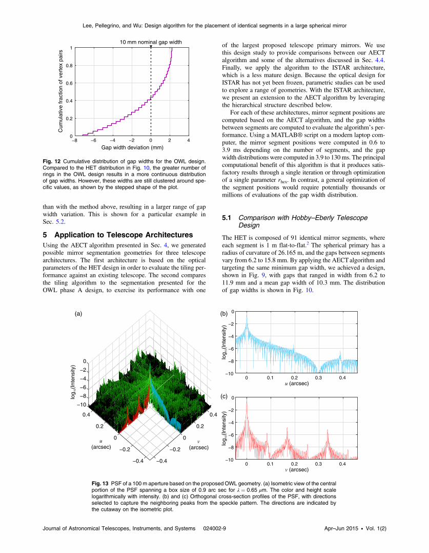
than with the method above, resulting in a larger range of gap

width variation. This is shown for a particular example in

Sec. 5.2.

5 Application to Telescope Architectures

Using the AECT algorithm presented in Sec. 4, we generated

possible mirror segmentation geometries for three telescope

architectures. The first architecture is based on the optical

parameters of the HET design in order to evaluate the tiling per-

formance against an existing telescope. The second compares

the tiling algorithm to the segmentation presented for the

OWL phase A design, to exercise its performance with one

of the largest proposed telescope primary mirrors. We use

this design study to provide comparisons between our AECT

algorithm and some of the alternatives discussed in Sec. 4.4.

Finally, we apply the algorithm to the ISTAR architecture,

which is a less mature design. Because the optical design for

ISTAR has not yet been frozen, parametric studies can be used

to explore a range of geometries. With the ISTAR architecture,

we present an extension to the AECT algorithm by leveraging

the hierarchical structure described below.

For each of these architectures, mirror segment positions are

computed based on the AECT algorithm, and the gap widths

between segments are computed to evaluate the algorithm’s per-

formance. Using a MATLAB® script on a modern laptop com-

puter, the mirror segment positions were computed in 0.6 to

3.9 ms depending on the number of segments, and the gap

width distributions were computed in 3.9 to 130 ms. The principal

computational benefit of this algorithm is that it produces satis-

factory results through a single iteration or through optimization

of a single parameter rhex. In contrast, a general optimization of

the segment positions would require potentially thousands or

millions of evaluations of the gap width distribution.

5.1 Comparison with Hobby–Eberly TelescopeDesign

The HET is composed of 91 identical mirror segments, where

each segment is 1 m flat-to-flat.2 The spherical primary has a

radius of curvature of 26.165 m, and the gaps between segments

vary from 6.2 to 15.8 mm. By applying the AECTalgorithm and

targeting the same minimum gap width, we achieved a design,

shown in Fig. 9, with gaps that ranged in width from 6.2 to

11.9 mm and a mean gap width of 10.3 mm. The distribution

of gap widths is shown in Fig. 10.

10 mm nominal gap width

0

0.6

0.8

1

Cum

ula

tive fra

ction o

f vert

ex p

airs

Gap width deviation (mm)

−8 −2

0.2

0.4

−6 −4 420

Fig. 12 Cumulative distribution of gap widths for the OWL design.Compared to the HET distribution in Fig. 10, the greater number ofrings in the OWL design results in a more continuous distributionof gap widths. However, these widths are still clustered around spe-cific values, as shown by the stepped shape of the plot.

−0.4

−0.2

0

0.2

0.4

−0.4

−0.2

0

0.2

0.4

−10

−8

−6

−4

−2

0

(a) (b)

(c)

0 0.1 0.2 0.3 0.4−10

−8

−6

−4

−2

0

0 0.1 0.2 0.3 0.4−10

−8

−6

−4

−2

0

u

(arcsec)v

(arcsec)

v (arcsec)

u (arcsec)

log

(Inte

nsity)

10

log

(Inte

nsity)

10

log

(Inte

nsity)

10

Fig. 13 PSF of a 100 m aperture based on the proposed OWL geometry. (a) Isometric view of the centralportion of the PSF spanning a box size of 0.9 arc sec for λ ¼ 0.65 μm. The color and height scalelogarithmically with intensity. (b) and (c) Orthogonal cross-section profiles of the PSF, with directionsselected to capture the neighboring peaks from the speckle pattern. The directions are indicated bythe cutaway on the isometric plot.



In this analysis and for the designs presented below, cumu-

lative distributions of the gap widths are used rather than histo-

grams in order to avoid sensitivity to binning. In each case,

perpendicular projected distances between vertex pairs are com-

puted as described in Sec. 4.3.1 and plotted in order of magni-

tude to obtain the cumulative distribution. The resulting gap

width distribution using the AECT algorithm has a 40% reduc-

tion in the total range compared to the original HET design.

Assuming a similar distribution of gap widths, the mean gap

width can be reduced by ∼20%, leading to a reduction in dif-

fraction effects as discussed earlier.

0

0.6

0.8

1

Cum

ula

tive fra

ction o

f vert

ex p

airs

Gap width deviation (mm)−15 0

AECT resultA,AB,ACA,B,ABA,C,AB

0.2

0.4

−10 −5 15105


Fig. 14 Cumulative gap width distributions based on the baselineazimuthal equidistant centroid tiling (AECT) algorithm and the threealternative tiling methods using spherical trigonometry. The legendindicates the angles and side lengths that are prescribed, basedon the notation in Fig. 7 and the spherical triangular tiling methodsdescribed in Sec. 4.4.

A,AB,AC A,B,AB A,C,AB

Spot radius (arcsec)

0 0.1 0.2 0.3 0.4 0.5 0.6 0.7 0.8 0.90

AE

CT

encircle

d e

nerg

y (

%)

99

0 0.1 0.2 0.3 0.4 0.5 0.6 0.7 0.8 0.9−0.6E

ncircle

d e

nerg

ydiffe

rence (

%)

0

0.2


90

99.9(a)

(b)

−0.2

−0.4

Fig. 15 Encircled energy profiles computed from the OWL PSFs.(a) Percent encircled energy of the baseline AECT design for theOWL configuration, plotted on a logarithmic vertical scale as a func-tion of spot radius in arc seconds for λ ¼ 0.65 μm. (b) Difference inencircled energy between the three spherical triangular tiling designsand the baseline AECT design, in percentage points. The legendindicates the angles and side lengths that are prescribed, based onthe notation in Fig. 7. One alternative design shows slightly greaterencircled energy than the AECT design, and the other two showmuch lower encircled energy in comparison.

10

0 m

5 m

Fig. 16 Hierarchical segment tiling configuration for the In-SpaceTelescope Assembly Robotics (ISTAR) design, with 19 segmentsin a module (left) and 271 modules in the full primary (right).Individual modules are shaded in alternating shades of gray for clarity.All segments are identical to each other, and all modules are alsoidentical to each other, which decreases the complexity of manufac-turing and assembly.

Gap w

idth

devia

tion (

mm

)

−2

−1

2

1

0

0

0.6

0.8

1

(a)

(b)

Cum

ula

tive fra

ction o

f vert

ex p

airs

Gap width deviation (mm)

−3

0.2

0.4

−2 −1 210


100 m

m n

om

inal gap w

idth

Fig. 17 Cumulative distribution of gap widths for the ISTAR design.(a) The total distribution of gap widths considering all adjacent seg-ments regardless of their module. Here the intramodule gaps are seenas the large near-vertical segment that appears at zero deviation fromthe nominal width. The intermodule gaps, considering adjacent seg-ments in different modules, comprise the remainder of the distributionand follows a trend similar to the OWL distribution. (b) The spatial con-figuration of intermodule gaps are plotted and color-coded based ondeviation from the nominal 100 mm gap width. Smaller gaps are plot-ted in red and larger gaps in blue. Note that gaps between adjacentrings remain large from the center to the edge, while the gaps betweenmodules in the same ring decrease in width from the center to theedge. Intramodule gaps are not plotted because of their small varia-tion relative to intermodule gaps.



5.2 Comparison with OWL Phase A Design

In the OWL phase A study, an optical configuration was pre-

sented for a 100 m spherical primary mirror with a 250 m radius

of curvature, composed of 3048 mirror segments with a flat-to-

flat dimension of 1.6 m (hexagonal side length of 0.92 m).13 The

design of this primary mirror included variable gap widths

ranging from 4 to 14 mm.

Using the proposed design algorithm with the OWL geom-

etry, a fully filled configuration including 33 rings was gener-

ated, as shown in Fig. 11.

This design includes 3367 segments filling the entire hexa-

gon, whereas the phase A design eliminated segments lying

outside the circular aperture or behind an obscuration, leaving

a total of 3048 segments. As a result, the distribution of gap

widths presented here is conservative relative to a more com-

plete design that accounts for removed segments. As discussed

in Sec. 4.3.1, the elimination of the central segments behind the

obscuration will result in a further reduction of the average gap

width. The cumulative distribution of gap widths, computed as

−0.4

−0.2

0

0.2

0.4

−0.4

−0.2

0

0.2

0.4

−10

−8

−6

−4

−2

0

0 0.1 0.2 0.3 0.4−10

−8

−6

−4

−2

0

(a)

(b)

(c)

0 0.1 0.2 0.3 0.4−10

−8

−6

−4

−2

0

u

(arcsec)v

(arcsec)

v (arcsec)

u (arcsec)

log

(Inte

nsity)

10

log

(Inte

nsity)

10

log

(Inte

nsity)

10

Fig. 18 PSF of a 100 m aperture based on the proposed ISTAR geometry. (a) Isometric view of thecentral portion of the PSF spanning a box size of 0.9 arc sec for λ ¼ 0.65 μm. The color and heightscale logarithmically with intensity. (b) and (c) Orthogonal cross-section profiles of the PSF, with direc-tions selected to capture the neighboring peaks from the speckle pattern. The directions are indicatedby the cutaway on the isometric plot.

−50

−20

−10

20

Gap w

idth

devia

tion (

mm

)

Primary radius of curvature R (m)

200

−40

−30

400 800600

Full range

1

Median

0

10

100 m

m g

ap w

idth

Fig. 19 Distribution of intermodule gap widths for ISTAR design as afunction of primary mirror radius of curvature. Because of the largefraction of intramodule gaps and their small variation relative to theintermodule gaps, we show only the intermodule gaps here. Aswas evident in the upward curvature of the point design cumulativedistributions above, the median and quartile values are biased towardthe upper end of the distribution. The total range satisfies the project-imposed constraint of 10% maximum deviation from the nominal100 mm gap only for mirror radius of curvature >400 m.

0

0.6

0.8

1

Cum

ula

tive fra

ction o

f vert

ex p

airs

Gap width deviation (mm)−3

0.2

0.4

−2 −1 210

100mm nominal gap width

Fig. 20 Cumulative distribution of gap widths for alternative ISTARdesign, minimizing the average gap width while keeping all gapslarger than the smallest in the original configuration. Here, the intra-module gaps appear at the bottom of the distribution, and the inter-module gaps comprise the upper curved portion of the distribution.



the vertex-to-vertex distance projected onto the normal direc-

tion, is shown in Fig. 12.

An average gap width of 10 mm was targeted by iteratively

modifying rhex, and a total range of 9 mm in gap width variation

was achieved, which is 10% better than the 10 mm range

reported in the OWL phase A study.

The PSF for this aperture was computed using a gray-pixel

bitmap image with 7.33 mm spatial resolution and 16-bit inten-

sity resolution. This imagewas padded to a total of 40,000 pixels

spanning a spatial dimension of 293 m. The central portion of

the computed PSF is shown in Fig. 13 as an isometric view with

two orthogonal cross-section profiles.

In order to compare the AECT design algorithm with alter-

natives using spherical trigonometry as described in Sec. 4.4,

each of the three competing spherical triangular methods was

used to compute a gap width distribution as well as PSFs.

Figure 14 shows a comparison of the gap width distributions,

with all three alternatives resulting in a wider range of gap

widths than the baseline AECT design.

Figure 15 compares the difference between the encircled

energy profiles of the baseline AECT design and the alternative

spherical triangular designs.

The second alternative method shows a slightly greater

encircled energy than the baseline design, despite the greater

range in gap widths. However, the other two alternatives show

much a lower encircled energy in comparison. Overall, the total

percentage point difference in encircled energy is less than half

a percentage point, which indicates a small effect on optical per-

formance. The total range of gap widths is likely a more signifi-

cant design driver, because the small range of the AECT design

allows for a more aggressive reduction of the mean gap width.

5.3 Proposed Hierarchical Design for ISTAR

The robotically assembled concept proposed for the ISTAR

project includes a 100 m spherical primary mirror assembled

from modules of mirror segments.14 An objective of the design

is to produce a mirror segment configuration that achieves

an average gap width of 100 mm with no greater than 10%

variation and to simplify the manufacturing and assembly proc-

ess by leveraging symmetry and modularity.

To achieve these goals, we developed a hierarchical exten-

sion to the AECTalgorithm, where the positions of 19 segments

were first computed to form a module with n ¼ 2 rings, and then

the module itself was treated as a larger hexagon and tiled to

form the primary with N ¼ 9 rings, totaling 5149 mirror seg-

ments. These are shown in Fig. 16. In order for the modules

to tile such that the individual segments align properly, the mod-

ule is rotated about its z axis by

ψmod ¼ tan−1!

1ffiffiffi

3p

ð2nþ 1Þ

#

þπ

2: (13)

The effective size of the module tiling hexagon is defined by

rmod ¼ rhex

ffiffiffiffiffiffiffiffiffiffiffiffiffiffiffiffiffiffiffiffiffiffiffiffiffiffi

3n2 þ 3nþ 1p

; (14)

and the spin and pitch angles are computed as described

in Sec. 4.2.

Because the modules span a relatively small solid angle

within the primary, there is very little variation in the intramod-

ule gaps, spanning a range of <2.5 μm. This results in a total

distribution, including both intermodule and intramodule

gaps, where a large fraction of the gaps is very close to the

desired gap width. In the ISTAR configuration, ∼75% of all

gaps are intramodule gaps, as can be seen in the distribution

in Fig. 17(a). The total range of gap width variation, however,

suffers slightly as a consequence, compared to a configuration

where all mirror segments are tiled in a single large array as in

the OWL design described in Sec. 5.2. Figure 17(b) shows how

the gap widths are spatially distributed over the surface of the

full primary. Because of the low variation of intramodule gaps,

only the intermodule gaps are plotted, showing the larger gap

widths near the center of the primary and the smaller gap widths

near the rim.

The PSF for this aperture was computed using the same tech-

nique described above for the OWL PSF. The central portion of

the computed ISTAR PSF is shown in Fig. 18 as an isometric

view with two orthogonal cross-section profiles. Because of

the imposed larger minimum gap width for robotic servicing,

diffraction effects are much greater than in the OWL design,

with speckle peaks approximately two orders of magnitude less

intense than the central peak, compared to almost five orders of

magnitude for OWL.

The design process was repeated for several values of the

primary radius of curvature R, ranging from 200 m up to the

baseline 800 m for the design described above. The range of

intermodule gaps, plotted in Fig. 19, shows that the gap varia-

tions increase slowly as R decreases from 800 down to 400 m,

but then grows more rapidly for smaller values of R. This para-

metric study demonstrated the value of using the AECT algo-

rithm to quickly produce viable mirror geometries, without the

need for intensive computation or optimization routines.

A feature of the hierarchical segmentation method is that an

extra degree of freedom is introduced by separately tiling first a

module and then the full mirror. This allows the gap width dis-

tribution to be manipulated. As discussed in Sec. 3.3, we would

ideally like to produce a tiling geometry that has minimum aver-

age gap width subject to constraints. In the hierarchical method,

we are able to more aggressively tile the segments within each

module and achieve a distribution very close to the minimum

Spot radius (arcsec)0 0.1 0.2 0.3 0.4 0.5 0.6 0.7 0.8 0.9

0

90

99

0 0.1 0.2 0.3 0.4 0.5 0.6 0.7 0.8 0.9−5E

ncircle

d e

nerg

ydiffe

rence (

%)

0

5

(a)

(b)


Baselin

eencircle

d e

nerg

y (

%)

Fig. 21 Encircled energy profiles computed from the ISTAR PSFs.(a) Percent encircled energy of the baseline AECT design for theISTAR configuration, plotted on a logarithmic vertical scale as a func-tion of spot radius in arc seconds for λ ¼ 0.65 μm. (b) Difference inencircled energy between the modified AECT design and the baselinedesign, in percentage points. The positive values at smaller spotradius indicate a higher percentage of encircled energy in the modi-fied design.



width constraint. The intermodule gap distribution would then

target a larger gap width in order to avoid violating this con-

straint. An example of a possible gap width distribution is shown

in Fig. 20. Here, the total range of gap widths has increased by

8.3% from 3.45 to 3.74 mm, but the average gap width has been

reduced from the original configuration by 1.4 mm. While the

original AECT scheme had an average gap width that was

2.07 mm (60% of the full range) above the minimum, this modi-

fication achieves an average gap width that is only 0.67 mm

(18% of the full range) above the same minimum.

Figure 21 shows the encircled energy of the original design

and the difference with the modified design. From this result, it

appears that the modified design has up to two percentage points

greater encircled energy at small radii, but that this effect does

not persist beyond a radius of ∼0.4 arc sec. Depending on the

imaging application, one design may be preferable over the

other, or a further parametric study using the AECT algorithm

can be applied to characterize the range of possible designs.

6 Conclusions

In this paper, we presented the AECTalgorithm to determine the

positions of identical hexagonal mirror segments on a spherical

surface. We used a one-dimensional analog to motivate the

desire for a small range in gap widths and to bias the mean

toward the low end of that range. We showed through compari-

son with HET and OWL designs that the algorithm compares

favorably to prior techniques in terms of the total range of

gap widths and presented a hierarchical concept based on the

ISTAR geometry that is effective for biasing the gap width dis-

tribution and could potentially lead to improved designs for

other large telescopes. The utility of the algorithm for use in

a parametric design study was also demonstrated using the

ISTAR concept.

From the one-dimensional analog, we verified that the PSF is

not strongly influenced by variation in gap width and also found

that the contrast performance could be enhanced by nonuniform

spacing. Through the design studies with three telescope configu-

rations, we showed that the AECT algorithm is capable of

satisfying mirror segment placement constraints over a wide

range of geometries and is well suited for use in early design

studies. The HET study demonstrated that the AECT design

could reduce the mean gap width by ∼20% compared to the

actual design. The OWL study demonstrated that the AECT

algorithm can handle several thousand individual segments and

showed a 10% reduction in total gap width range from the pre-

viously reported design. The ISTAR study demonstrated several

approaches for using the AECTalgorithm for preliminary design.

In future work, the AECT algorithm would also be a viable

candidate to provide starting points for optimization of a final

design. As future ground- and space-based telescopes target

increasingly large apertures, the need for computationally effi-

cient design algorithms will become more essential in order to

manage the large number of mirror segments required.

Acknowledgments

We thank Marie Laslandes for helpful discussions and James

Breckinridge for valuable and detailed feedback about the

manuscript. N. Lee was supported through this work by a post-

doctoral fellowship from the W. M. Keck Institute for Space

Studies. The research was carried out in part at the Jet Propul-

sion Laboratory, California Institute of Technology, under a con-

tract with the National Aeronautics and Space Administration.

References

1. J. E. Nelson, T. S. Mast, and S. M. Faber, “The design of the Keck

Observatory and Telescope,” Technical Report Keck Observatory

Report No. 90, Caltech (1985).

2. V. L. Krabbendam et al., “Development and performance of Hobby–

Eberly Telescope 11-m segmented mirror,” Proc. SPIE 3352, 436–445

(1998).

3. R. Stobie, J. G. Meiring, and D. A. H. Buckley, “Design of the Southern

African Large Telescope (SALT),” Proc. SPIE 4003, 355–362 (2000).

4. P. A. Sabelhaus and J. E. Decker, “An overview of the James Webb

Space Telescope (JWST) project,” Proc. SPIE 5487, 550–563 (2004).

5. M. Postman et al., “Advanced Technology Large-Aperture Space

Telescope: science drivers and technology developments,” Opt. Eng.

51(1), 011007 (2012).

6. C. Baffes et al., “Primary mirror segmentation studies for the Thirty

Meter Telescope,” Proc. SPIE 7018, 70180S (2008).

7. Y. Chu, “The large sky area multi-object fibre spectroscopy telescope

(LAMOST) project,” in Wide-Field Spectroscopy, E. Kontizas et al.,

Eds., Vol. 212, pp. 67–72, Springer, Netherlands (1997).

8. L. Jochum, J. Castro, and N. Devaney, “Gran Telescopio Canarias: cur-

rent status of its optical design and optomechanical support system,”

Proc. SPIE 3352, 621–631 (1998).

9. T. Andersen et al., “The Euro50 extremely large telescope,” Proc. SPIE

4840, 214–225 (2003).

10. T. S. Mast and J. E. Nelson, “Segmented mirror control system hardware

for CELT,” Proc. SPIE 4003, 226–240 (2000).

11. J. Nelson and G. H. Sanders, “TMT status report,” Proc. SPIE 6267,

626728 (2006).

12. European Southern Observatory, “The E-ELT construction proposal,”

Technical Report, ESO (2011).

13. European Southern Observatory, “OWL concept design report: phase A

design review,” Technical Report OWL-TRE-ESO-0000-0001, ESO

(2005).

14. K. Hogstrom et al., “A robotically-assembled 100-meter space tele-

scope,” presented at International Astronautical Congress, IAC-14-

C2.2.6, International Astronautical Foundation, Toronto, Canada (2014)

15. M. Laslandes et al., “Optimization of electrode configuration in surface-

parallel actuated deformable mirrors,” Proc. SPIE 9148, 914843 (2014).

16. J. Steeves et al., “Design, fabrication and testing of active carbon shell mir-

rors for space telescope applications,” Proc. SPIE 9151, 915105 (2014).

17. L. Jolissaint and J.-F. Lavigne, “An analytic model for the study of the

impact of mirror segmentation on AO performance and application to

a 30-m segmented telescope,” Proc. SPIE 5497, 349–360 (2004).

18. G. Chanan et al., “Control and alignment of segmented-mirror tele-

scopes: matrices, modes, and error propagation,” Appl. Opt. 43(6),

1223–1232 (2004).

19. D. O’Donoghue, “Correction of spherical aberration in the Southern

African Large Telescope (SALT),” Proc. SPIE 4003, 363–372 (2000).

20. K. Matthews et al., “The first diffraction-limited images from the W. M.

Keck Telescope,” Publ. Astron. Soc. Pac. 108(725), 615–619 (1996).

21. J. W. Goodman, Introduction to Fourier Optics, McGraw-Hill Series in

Electrical and Computer Engineering, 2nd ed., McGraw-Hill, New York

(1996).

22. E. Hecht, Optics, 4th ed., Addison-Wesley Publishing Company, San

Francisco, California (2001).

23. N. Yaitskova, K. Dohlen, and P. Dierickx, “Analytical study of diffrac-

tion effects in extremely large segmented telescopes,” JOSA A 20(8),

1563–1575 (2003).

24. J. B. Breckinridge, Basic Optics for the Astronomical Sciences, SPIE

Press, Bellingham, Washington (2012).

25. C. Nissly et al., “High-resolution optical modeling of the Thirty Meter

Telescope for systematic performance trades,” Proc. SPIE 7017,

70170U (2008).

26. M. Troy and G. Chanan, “Diffraction effects from giant segmented-

mirror telescopes,” Appl. Opt. 42(19), 3745–3753 (2003).

27. D. Spergel et al., “Wide-field infrared survey telescope-astrophysics

focused telescope assets WFIRST-AFTA final report,” Technical

Report, WFIRST Project (2013).

Nicolas Lee is a W. M. Keck Institute for Space Studies postdoctoralscholar in aerospace at Caltech and received his PhD in aeronauticsand astronautics from Stanford University in 2013. Current research



http://dx.doi.org/10.1117/12.319265

http://dx.doi.org/10.1117/12.391525

http://dx.doi.org/10.1117/12.549895

http://dx.doi.org/10.1117/1.OE.51.1.011007

http://dx.doi.org/10.1117/12.790206

http://dx.doi.org/10.1117/12.319300

http://dx.doi.org/10.1117/12.458049

http://dx.doi.org/10.1117/12.391512

http://dx.doi.org/10.1117/12.672937

http://dx.doi.org/10.1117/12.2056495

http://dx.doi.org/10.1117/12.2056560

http://dx.doi.org/10.1117/12.552551

http://dx.doi.org/10.1364/AO.43.001223

http://dx.doi.org/10.1117/12.391526

http://dx.doi.org/10.1086/133773

http://dx.doi.org/10.1364/JOSAA.20.001563

http://dx.doi.org/10.1117/12.788596

http://dx.doi.org/10.1364/AO.42.003745

interests include deployable space structures, small spacecraft sys-tems, and space environmental monitoring.

Sergio Pellegrino is the Joyce and Kent Kresa professor of aeronau-tics and professor of civil engineering at Caltech and a Jet PropulsionLaboratory senior research scientist. He received his laurea in civilengineering from the University of Naples in 1982 and his PhD instructural mechanics from the University of Cambridge in 1986. His

general area of research is the mechanics of lightweight structures,with a focus on packaging, deployment, shape control, and stability.

Yen-HungWu received his MS in optical engineering in 2007 from theUniversity of Arizona. Since 2007, he has been a staff engineer at theJet Propulsion Laboratory, California Institute of Technology. He is amember of the Optical Design & Engineering group and was the opti-cal and opto-mechanical engineer for the NuSTAR metrology laser.



Multi-Layered Membrane Structures with Curved Creases for

Smooth Packaging and Deployment

Nicolas Lee∗ and Sergio Pellegrino†

California Institute of Technology, Pasadena, CA 91125

We present a design for a deployable multi-layered membrane structure that uses a curved crease pattern

to enable smooth wrapping around a spool. The crease pattern is parameterized to enable a variety of designs,

and a specific implementation was selected based on an existing patch antenna array design. We constructed a

prototype structure based on this geometry, and conducted deployment tests to measure the deployment force

profile required to unfold the structure and to unwrap it from a spool. We find that the deployment force

for unwrapping is significantly higher than for unfolding. These force profiles are repeatable over multiple

deployments and the global trends do not depend on deployment rates over the range tested, between 1 and

8 mm/s. However, the local dynamic behavior can depend on deployment rate.

I. Introduction

In this paper, we present a design for a multi-layered membrane structure that can be deployed from a cylindri-

cal spool. This type of deployable membrane structure has potential applications in spacecraft systems. Deployable

systems in general are a crucial aspect of spacecraft design because of their ability to address and satisfy constraints

imposed during different mission phases. During launch, the rocket fairing and the acoustic environment impose geo-

metric and stiffness constraints that are often incompatible with the performance requirements for large area systems

during the operational phase. Maximizing the area of a spacecraft component is essential for many systems where

performance is directly related to a captured flux quantity. Obvious examples include solar arrays and communica-

tions antennas, but deployed area is also a factor for systems including but not limited to telescopes, radar, and in situ

dust detectors and collectors. While many spacecraft use deployable technology, it remains a significant risk with a

history of many failures and anomalies. These include jammed solar panel hinges (e.g. Intelsat 191) and dish antennas

(e.g. Galileo’s high gain antenna2 and SkyTerra 1’s 22-meter L-band antenna3), incomplete tether deployments (e.g.

MAST4), and broken tethers and booms (e.g. ARTEMIS, TSS-1R5). Membrane systems in particular are prone to

unexpected behavior during deployment, including for example the tearing of the Znamya 2.5 solar reflector,6 and

premature expansion of components of the Inflatable Antenna Experiment.7 The dependence of future spacecraft

on deployable systems necessitates a better understanding of their behavior through all mission phases in order to

characterize and reduce overall mission risk.

Deployable spacecraft systems can range from extremely lightweight, such as solar sails that use membranes only

several microns thick, to relatively thick rigid panels such as the solar arrays deployed on communications satellites.

For some applications, the rigidity of a panel is not required and the complexity of hinges undesirable. In some

cases, like proposed large radar arrays for Earth observation, discrete panels are too heavy to be feasible but the thin

membranes used in solar sails are too thin to support the electronic components associated with each antenna.

In this paper, we present a design for a deployable thick-membrane structure for applications that require an

intermediate solution between thin membranes and rigid panels, using a membrane that is thick enough to support

electronics but is thin enough to be flexible. In particular, we focus on the implementation of a planar structure that

is compatible with an existing design for a membrane patch antenna array for synthetic aperture radar (SAR), as

illustrated in Figure 1. This structure is composed of two parallel membrane surfaces joined to each other by a set of

ribs that determine the thickness of the structure. The membranes are creased using a curved design to enable tight

packaging around a hub such that the structure can be packaged for launch into a volume with dimensions smaller

∗W. M. Keck Institute for Space Studies Postdoctoral Scholar, Graduate Aerospace Laboratories, 1200 E. California Blvd. MC 301-46.

[email protected]†Joyce and Kent Kresa Professor of Aeronautics and Professor of Civil Engineering, Graduate Aerospace Laboratories, 1200 E. California Blvd.

MC 301-46. AIAA Fellow. [email protected]

1 of 20

American Institute of Aeronautics and Astronautics

Figure 1. Rendering of a 6U CubeSat concept with membrane antenna array. In this image, the membrane antenna is shown with 16

patch antenna elements and is supported by a longitudinal boom. The membrane would theoretically deploy out of a 3U volume, with the

spacecraft bus occupying the other 3U. Background image courtesy NASA.

than the length of an uncreased panel. The full structure is 29.2 cm in width and 124.8 cm in length, with a 1.27 cm

separation between the two layers. A full-size prototype structure was constructed (Figure 2) and used to conduct

deployment experiments.

Through these experiments, we found that the dominant force resisting deployment as the structure is unfolding

results primarily from the unwrapping of the membrane from a hub, but that this deployment force can be exceeded

by the tension required at the end of deployment to ensure that the structure is adequately flat. The measured force

profiles were repeatable over multiple deployments and the global trends did not appear to depend on deployment rates

over the range tested, between 1 and 8 mm/s. We also found that the deployment rate can affect the dynamic behavior

of the membrane, even at relatively low rates.

Section II provides an overview of relevant background to the work described in this paper. Section III describes

mathematically the crease pattern used to enable smooth wrapping of the folded structure on a cylindrical hub, includ-

ing a general derivation for a parameterized structure with arbitrary dimensions and a specific design for the antenna

array configuration. Section IV presents the techniques used to assemble a prototype membrane structure consistent

with the geometry of the design from Section III. Deployment experiments that characterize the force profile using the

prototype in a materials testing machine are described in Section V, with results presented and discussed in Section VI.

Finally, Section VII provides a summary of the key findings and directions for further work in this area.

II. Background

This section highlights previous work on membrane packaging and deployment, as well as on the existing mem-

brane antenna array configuration that our membrane structure is designed to support.

A. Membrane Packaging and Deployment

Previous work on membrane packaging and deployment spans the range between theoretical models and empirical

observations. In particular, much work has been done on the problem of wrapping a membrane around a hub. Guest

and Pellegrino8 provided an algorithm for a crease pattern to wrap a membrane around a polygonal hub by determining

the 3D geometry of the crease vertices. Furuya et al.9 described experiments in centrifugal deployment of a wrapped

membrane from a spinning hub. Recently, Zirbel et al.10 performed experiments demonstrating the deployment of a

membrane with embedded rigid panels from a polygonal hub.

In order to enable wrapping around a round hub, Lee and Close11 presented an algorithm to compute a crease

pattern composed of equally spaced curved creases. In that work, creases are restricted to lie on a horizontal plane as

they are wrapped around the hub. This paper extends the technique to account for the more general case where creases

may not lie only on a horizontal plane. The crease pattern is applied to a membrane geometry such that multiple

membrane layers can be attached to each other at a specified distance to form a thicker global structure once deployed.

This membrane structure design is targeted to support a planar patch antenna array described in the following section.

2 of 20


Figure 2. Prototype membrane structure in several stages of deployment. (a) The packaged structure can be coiled into a package with

diameter less than 10 cm. (b)-(e) As the membrane unfolds, it flattens into a structure 29.2 cm in width and 124.8 cm in length with the two

membranes separated by 1.27 cm.

3 of 20


B. Membrane-based Patch Antenna Array

A phased array patch antenna system has been developed at the Jet Propulsion Laboratory for L-band (1.26 GHz)

SAR applications.13 These antenna systems are envisaged for Earth-observation missions at medium or geostationary

Earth orbit (MEO or GEO), where larger arrays are required than at low Earth orbit (LEO). The higher altitude allows

for revisit times on the order of minutes suitable for disaster response or future study of earthquake physics.12

Active arrays of up to 256 elements (in a 16 × 16 rectangular array) have been tested using phase-shifting trans-

mit/receive (T/R) modules to electronically steer the main beam up to 30◦.13 This antenna array is composed of two

membrane layers, with the radio frequency feed network, T/R electronics and ground plane on one membrane, and

radiating patches on the other. Slots in the ground plane allow the feed network to couple with the radiating patches

so that no physical electrical connection is required between the layers. The patch elements are 8.89 cm (3.5”) square,

positioned in a rectangular array with a spacing of 15.24 cm (6”). Previous passive antenna designs have also used a

three-layer configuration so that the feed network is placed a greater distance away from the ground plane.14

These prototypes were designed with 50 µm DuPont™ Kapton® polyimide filma as the membrane substrate. Thin-

ner membranes would require a corresponding decrease in the width of the feed network to maintain impedance, and

is limited by fabrication constraints. The most recent prototypes have used conventional flexible printed circuit board

(PCB) fabrication techniques by etching a copper foil layer. Potential avenues for overcoming this constraint could

involve alternative circuit fabrication techniques, such as materials printing with conductive inks.

We used the existing two-layer antenna array design to motivate the development of the multi-layered membrane

structure described in this paper. This deployable structure, using the crease pattern described in the next section,

provides one possible approach toward implementing the antenna array as a spacecraft payload.

III. Membrane Crease Design

In order to allow the membrane structure with multiple layers to collapse and lie flat, we chose to use the same

crease pattern on all layers. The crease pattern for each membrane is based on the beech leaf fold described by

Kobayashi et al.15 and shown in Figure 3. In this section, we describe the general parameters governing the folding

behavior of this crease pattern, as well as the modifications necessary to allow the folded membrane to wrap smoothly

around a spool while accounting for the membrane thickness τ. We then describe the specific crease pattern selected

to be compatible with the antenna array design. Finally, we discuss alternative possibilities for arranging multiple

membrane layers in the structure.

Figure 3. Kobayashi’s beech leaf folding pattern with relevant parameters illustrated. Valley folds are denoted with dashed lines and

mountain folds with dash-dotted lines. Parameters that can be varied include the crease spacing p and the crease angle ψ.

A. General Crease Pattern

The beech leaf folding pattern has two sets of diagonal creases. Each crease intersects with one from the opposite

set at a centerline crease, which alternates between mountain and valley folds. The fold pattern is determined only

by the spacing between the diagonal creases and by the angle they make with the centerline crease. This angle ψ

between the centerline crease and the diagonal creases is constrained between 0◦ and 90◦, with 0◦ corresponding

to the degenerate case where the diagonal creases are parallel to the centerline and folding does not occur, and 90◦

corresponding to the case of maximum longitudinal compression along the centerline. To attach membrane layers

to each other, vertical ribs can be attached along the diagonal creases. However, this requires that the crease angles

remain constant so that the creases are parallel. The crease separation distance p is also usually constant and can be

selected to provide a height p sinψ of the folded membrane configuration.

aDuPont™ and Kapton® are trademarks or registered trademarks of E.I. du Pont de Nemours and Company

4 of 20


By keeping the parameters constant over all creases, the folded configuration will have a uniform height, which

simplifies the packaging process. Additionally, for some applications such as solar panels, components of a constant

size must be embedded on the membrane between creases, and is more straightforward to implement on a membrane

with creases at a constant spacing. However, by allowing the crease angles and separation distances to vary, it is

possible to achieve favorable deployment dynamics. The kinetic energy associated with deployment varies as the

deployment angle θ goes from 0◦ to 90◦, and is greatest near the end of deployment when θ ≈ 90◦.16 With a folding

pattern that has smaller crease angles at the root of the membrane and larger angles at the tip, the deployment energy

profile can be tuned for greater uniformity.

The straight line crease patterns can then be adapted using curved creases to coil smoothly so that they can be pack-

aged on a spool. The technique to determine the crease curvature has been developed previously by Lee and Close11

and is based on the principle of computing the crease length in the coiled configuration to determine its required

curvature in the unfolded configuration. A similar finding was determined through empirical folding experiments by

Satou and Furuya.17 However, the algorithm needs to be adapted to the properties of this particular crease pattern.

Specifically, the reference center line for the beech leaf crease pattern does not remain horizontally in the same plane;

it zig-zags across the height of the pleat as depicted in Figure 4. This produces a longitudinal compression in the

folded membrane, and results in a crease that must lie along a helical spiral in the coiled configuration.

Figure 4. Sketch of the curved crease geometry in its (a) wrapped and (b) flattened configurations. The center line crease (in red) traverses

along helical spiral segments as the membrane wraps around a hub. The diagonal creases (in blue) remain in a horizontal plane, but

alternate creases lie on different planes.

For a structure geometry where the length is greater than the width, we can assume that the thickness of the folded

membrane configuration is roughly constant and can approximate the coiled radius of the centerline as an Archimedes’

spiral of the form

r(θ) = r(0) +r(2π) − r(0)

2πθ = r(0) + bθ, (1)

where θ is the angular coordinate around the hub, b is the spiral rate parameter, and r(0) is the initial radius. For a

total folded thickness 2h, we have the rate parameter b = h/π. However, unlike the previous work, the path length of

the crease must be projected in 3D such that

ξ(θ) cosψ =(bθ + r(0))

p

b2 + (bθ + r(0))2

2b

+1

2b ln

p

b2 + (bθ + r(0))2 + bθ + r(0)p

b2 + r(0)2 + r(0)

−

r(0)p

b2 + r(0)2

2b,

(2)

where the right-hand side is the closed form path length of the Archimedes’ spiral. The curvature of the spiral is

κ =(2 + (θ + r(0)/b)2)

b(1 + (θ + r(0)/b)2)3/2, (3)

5 of 20


which can be related to the crease radius of curvature R using the relation

R =

✓

p

τ

◆

1

κ. (4)

The diagonal creases in the folding pattern do remain in a horizontal plane when the membrane is folded, and their

curvature is therefore described as above but without the cosψ projection.

Figure 5 contains a folding pattern developed using this algorithm. A similar pattern was used to fold the paper

model in Figure 6, which demonstrates the ability of the folded membrane to wrap tightly and smoothly. To assess the

effectiveness of this folding strategy, the packing efficiency is estimated as the volume of membrane material divided

by the smallest volume of an encompassing rectangular prism. A paper membrane with an area of 400 cm2 and

thickness of 0.11 mm has a volume of 4.4 cm3, and was packaged into a roll with a diameter of 2.3 cm and a height of

1.5 cm, which can be contained within a rectangular volume of 7.94 cm3. This is a packing efficiency of 55%, which

includes volumes within the spool and in the corners of the box that remain usable.

B. Crease Pattern for Membrane Antenna Array

With the membrane antenna array described in Section II.B, a practical consideration is that the creases may

degrade the performance of the antenna by affecting the geometry or even the conductivity of the radiating elements.

Additionally, the existing design uses T/R modules that could not be creased with the membrane. We therefore

designed a crease pattern choosing parameters that would avoid creases overlapping with either the T/R modules or

the patches. The goal for this design was to fit a 2 × 8 array onto a membrane that could package inside a 3U CubeSat

volume (10 × 10 × 34.5 cm). With the 15.24 cm antenna spacing in two dimensions, a rigid-foldable pattern based

around the patches, where individual panels do not bend, would not fit within the prescribed volume. However, the

Figure 5. Beech leaf folding pattern with curved creases to enable wrapping in the folded configuration. Valley folds are denoted with

dashed lines and mountain folds with dash-dotted lines. In this crease pattern, the crease angle ψ has been chosen to be 45◦ .

Figure 6. Paper prototype of a two-layer structure using a curved beech leaf crease pattern. These three photos show (a) the initial

wrapped membrane, (b) an intermediate stage during deployment, and (c) the final deployed structure.

6 of 20


use of the curved crease pattern permits one linear dimension to wrap around a spool, while the other can occupy the

longest dimension of the CubeSat volume.

For this crease design, the free parameters available in the design space include the crease angle ψ, the spiral

parameter b, and the spool radius r0. In order to fit the diagonal creases between the patches, the angle ψ must be

greater than 54◦. However, having a large crease angle will result in a thicker folded membrane package, which would

be more difficult to coil. A crease angle of 75◦ was selected as a compromise between these two competing objectives.

The spiral parameter was computed by estimating a total folded membrane thickness of 4 mm, accounting for the

additional thickness necessary to embed electronics on the surface. This yields a spiral rate of 4 mm per revolution,

or 0.64 mm per radian. Because of the limited space between the two rows of patches, we desired a centerline crease

with as little curvature as possible. This was accomplished by selecting the largest possible spool radius that would

result in a wrapped membrane still satisfying the 10 × 10 cm CubeSat constraint. These geometric constraints are

depicted in Figure 7. A spool radius of 4 cm was found to be adequate to satisfy the design requirements. Using these

parameters, the curved crease pattern was produced, and overlaid on the rectangular patch antenna array, as shown in

Figure 8.

Figure 7. Antenna array dimensions and constraints on crease geometry. Each radiating patch is a square with a side length of 8.89 cm.

The patches are spaced in a rectangular array at intervals of 15.24 cm in both directions. In order to avoid creasing the patch, the minimum

crease angle possible using a straight-line beech leaf crease pattern is approximately 54◦ . When implementing a curved crease pattern, the

centerline must lie within the 6.35 cm gap between patches.

C. Arrangement of Multiple Membrane Layers

Using the beech leaf folding pattern with a constant crease angle, the diagonal creases remain parallel and horizon-

tal as the membrane folds. The corresponding diagonal creases on parallel membranes with the same crease pattern

would therefore remain the same distance apart. In order to construct a multi-layered structure, these diagonal creases

can be joined by a vertical rib. As the membrane structure folds, each of the rectangular cells formed by two horizontal

membrane panels and the two ribs connecting them would be able to shear and flatten and the two membranes will

nest inside each others folds. The overall thickness of the structure and the spacing between the membranes can be

arbitrarily selected by choosing the appropriate rib height.

However, it is not necessary to place ribs on every diagonal crease, or even only on the creases. Depending on the

geometry of the structure and the stiffness of the materials used, it may be more appropriate to place ribs at every other

crease if the crease spacing is small, or to add additional ribs in between creases if the crease spacing is large. If ribs

are placed only at ever other crease, then they will all stack together in the folded structure rather than in two separate

groups in the case of ribs at every crease. If additional ribs are necessary, the design would be equivalent to reducing

the diagonal crease spacing in the pattern but leaving some of these creases unfolded.

In the case of a two-layer membrane, another alternative arrangement would be to have the membranes folded in

an opposite sense, with valley folds on one membrane corresponding to mountain folds on the other, and vice versa.

7 of 20


Figure 8. Design for a crease pattern compatible with the antenna array geometry. (a) Packaged configuration showing the centerline

crease in red, the round spool (4 cm radius) in gray, and the CubeSat constraints (10 cm square). (b) The crease pattern with antenna

components. The centerline crease is shown in red, the radiating patches in blue, and the T/R modules in green. Valley folds are denoted

with dashed lines and mountain folds with dash-dotted lines.

This would result in a more symmetrical but taller folded package. This could be beneficial if certain parts of the

membrane cannot be folded against each other or if the membrane contains thicker elements that do not stack well in

the folded package.

IV. Prototype Fabrication

We used the crease pattern described in the previous section to construct a prototype membrane structure that could

support a 2 × 8 patch antenna array based on the JPL design described in Section II.B. This prototype was constructed

using 50 µm thick Kapton® polyimide film to be consistent with the JPL design. In order to assemble the components

of the structure, we chose to use a continuous membrane for one layer, and to cut the other layer into separate panels

based on the locations of the ribs. The ribs were attached first to the continuous layer, and then the second layer was

attached segment by segment onto the ribs. This is representative of a potential assembly process for the antenna array,

since the design includes one continuous layer with the feed network and ground plane, while the other layer only has

radiating patches that do not require a physical electrical connection (such as a wire or microstrip trace) to the other

membrane or to other locations within the same membrane.

Because of the geometry for this particular design, where the rib length is short relative to the rib spacing, there is

a greater tendency for the membrane layers to buckle between the ribs than if the ribs were more closely spaced. To

mitigate this effect, thin carbon fiber rods (0.50 mm diameter) were used to stiffen the edges of the membrane. These

rods were cut to length based on the crease length of each segment, and were attached along the edges as well as on

the longitudinal crease down the center of the structure. Each rod was bonded to the membrane using cyanoacrylate

adhesive at the end points and the middle. The rods along the edge of the structure were reinforced with small tabs of

polyimide tape to prevent delamination from the membrane. Photos of the prototype fabrication process are included

in Figure 9.

The prototype design demonstrated qualitatively good ability to fold and wrap. In total, it was 59 g in mass and

covered an area of 0.35 m2. This areal density of 0.7 kg/m2 does not include any supporting structure or the hub,

but is very promising in reducing the mass of large planar structures from the current state-of-the-art rigid panel

technologies. In order to quantify the deployment behavior of this structure, we conducted deployment experiments

with a force sensor, described in the following section.

8 of 20


Figure 9. Membrane structure fabrication. (a) The bottom membrane layer is a continuous sheet of Kapton® while the top layer is

separated into eight panels. (b) Ribs are attached to the bottom layer with short segments of polyimide tape. The top panels are attached

in a similar manner to the ribs. (c) Thin carbon rods are attached on the edge of the membrane structure and along the centerline crease

in order to stiffen the individual panels. (d) The completed membrane structure.

9 of 20


V. Deployment Experiments

To study the deployment force profile of the membrane structure described in Section IV, the prototype was

deployed using a materials testing machine. In order to characterize the forces associated with unwrapping the mem-

brane from a spool, two configurations were tested: the membrane was deployed first from a folded state without being

wrapped around a spool, and then from a wrapped and folded state around a rotating hub.

An Instron model 5569 materials testing machine was used to perform the deployment experiments. Because the

total length of the membrane structure exceeded the total length of travel of the machine, different configurations were

used to study the deployment. The load cell used (model 2525-808) has a range of ±10 N, with accuracy better than

2.5 mN for indicated loads below 1N, or 0.25% of the indicated load for values greater than 1 N.18 The load cell can

be sampled at an adaptive rate depending on the slope of the previous measurements, up to a maximum of 500 Hz.

The membrane was attached to the load cell using a screw and nut, with a total mass of 4.6 g, connected to a short

tab at the tip (midpoint of the deployed end) of the membrane structure. For the unfolding configuration, the root of

the membrane structure was fixed to the table surface in front of the machine (28 cm forward and 19 mm below the

base of the machine’s lowest point of travel). By anchoring the structure below the base of the machine, we were

able to capture the end of deployment before reaching the upper limit of travel. However, at the start of the test, the

membrane was already deployed to a length of 37 cm. Figure 10 shows the setup for this deployment configuration.

For the unwrapping configuration, a spool was mounted in the machine, centered below the load cell and with the

axis of rotation horizontal and 10 cm above the machine’s lowest point of travel. The spool is a 5.08 cm (2”) diameter

aluminum tube with plastic conveyer roller end caps mounted via bushings onto a threaded rod. The mass of the

rotating part of the spool is 163.1 g. In order to prevent the membrane structure from unwinding off the spool, it was

necessary to impart an external moment on the spool. This was implemented using the counterweight of a 100 g mass

on a string, with a pulley used to allow the weight to extend beyond the edge of the table. The string was attached to

the surface of the spool and wrapped around it in the opposite direction as the membrane structure. A schematic of the

unwrapping configuration is shown in Figure 11 with photos of the setup in Figure 12. Neglecting the transient effect

of accelerating the mass up and down as the spool rotates, this configuration provided a constant 25 mNm torque on the

spool. Because the spool for the unwrapping configuration is mounted closer to the load cell than the root anchor point

in the unfolding configuration, the deployments could start at a deployed length of 10 cm, but could only deploy to a

length of 100 cm and not reach the fully deployed length of 125 cm. Deployments were performed at constant speeds

ranging from 1 mm/s to 8 mm/s with force measurements sampled at the maximum rate of 500 Hz. During several

deployments, video was captured simultaneously. In this paper, results will be discussed from fifteen deployments:

eight that were performed from the unfolding configuration, and seven from the unwrapping configuration.

Figure 10. Photo of the membrane structure deployed from the unfolding configuration. The root of the structure was attached to the

table in front of the materials testing machine. The tip was attached to the load cell in the machine.

10 of 20


Figure 11. Drawing of the components in the unwrapping configuration. The membrane was attached at the tip to the load cell, and at

the root to a spool. The spool was attached to a counterweight through a pulley in order to keep the membrane from unwinding around the

spool.

Figure 12. Two photos of the experimental setup for the unwrapping configuration, from the (a) front and (b) back of the materials testing

machine. The counterweight and pulley can be seen at the back of the machine. An aluminum plate was used to provide a smooth base

from which to deploy, so that the membrane would not catch on the fixtures present below the plate.

11 of 20


VI. Experimental Results

With the data collected as described in the previous section, the force profiles for the deployments showed several

notable characteristics. The raw measurements are shown in Figure 13. First, the unfolding configuration resulted in

a gradual increase in the measured deployment force with a transition to a sharper increase near the end. The gradual

increase is attributed primarily to the self weight of the membrane. Second, the unwrapping configuration resulted in a

deployment force profile that has several peaks corresponding to the unfolding of the lateral creases in the membrane

structure. Finally, during the portions of the unwrapping deployment where the force is generally decreasing, the

shape of the force profile is punctuated by a characteristic sawtooth shape with a rapid drop followed by a gradual

increase. This can be seen in Figure 14, which shows the deployment force profile for an unwrapping deployment at a

rate of 1 mm/s. There is one particular unfolding panel where this does not occur; this anomalous behavior occurred

consistently over multiple deployments at a deployment length of 50 to 70 cm, always on the fourth out of seven panels

deployed. The data were adjusted to account for disturbances and biases, including the self weight of the membrane

and the moment applied to the spool. These were both approximated as linear functions with respect to deployed

length. The corrected measurements are shown in Figure 15. Figure 16 shows one unfolding and one unwrapping

deployment force profile, along with images of the deployment at 20 cm intervals.

In the following sections, we will look first at the global deployment force profile and how it varies throughout the

deployment for the two experimental configurations, and then analyze in more detail the local dynamic behavior that

can be seen in some of the measurements.

A. Global deployment force profile

The deployment force profiles appear quite different for the wrapped and unwrapped configurations. When the

membrane is only folded but not wrapped around the hub, the deployment force remains quite small and relatively

constant. When it is wrapped around the hub, a periodic spike in the deployment force appears, corresponding to

the periodicity of the crease pattern. The reason for this increased deployment force compared to the unfolding

configuration is that the crease pattern is derived from a Miura-ori design.20 In a conventional Miura-ori fold pattern,

the folded membrane behaves as a single degree-of-freedom mechanism: all panels unfold simultaneously. However,

0 0.2 0.4 0.6 0.8 1 1.20

0.5

1

1.5

Deployed length [m]

Fo

rce

[N

]

Unfolding

Unwrapping

Figure 13. Plot of raw force measurements for all deployments with respect to deployed length. This includes eight unfolding deployments

and seven unwrapping deployments.

12 of 20


0.38 0.4 0.42 0.44 0.46 0.48 0.50.45

0.5

0.55

0.6

0.65

0.7

0.75

Deployed length [m]

Fo

rce

[N

]

Figure 14. Plot of force measurements for an unwrapping deployment at 1 mm/s. From a deployed length of 37 cm to approximately

47 cm, the deployment force shows a global decrease with characteristic transient features. From 47 cm to 50 cm, the deployment force

increases globally and shows fewer of the transients.

0 0.2 0.4 0.6 0.8 1 1.2

0

0.2

0.4

0.6

0.8

1

Deployed length [m]

Fo

rce

[N

]

Unfolding

Unwrapping

Figure 15. Plot of corrected force measurements for all deployments with respect to deployed length. This includes eight unfolding

deployments and seven unwrapping deployments and have been adjusted to remove the effect of self weight of the membrane structure,

and for the unwrapping configuration also the effect of the counterweight.

13 of 20


Figure 16. Plot of corrected force measurements for two deployments with respect to deployed length, with photos of the deployed

membrane structure. The unfolding deployment, shown in red with the photos below the plot, was performed at 5 mm/s. The unwrapping

deployment, shown in blue with the photos above the plot, was performed at 4 mm/s. The photos are shown at equally spaced intervals of

20 cm deployed length for each of the configurations.

14 of 20


in this curved design, the spool prevents the wrapped portion of the structure from unfolding. As a result, each panel

must be peeled away from the adjacent panel on the spool, resulting in significant buckling of the membrane surface.

As these buckles propagate and the panel lifts off of the spool, the deployment force decreases until the next panel

starts to peel away from the spool and the cycle repeats.

The peeling behavior of the wrapped membrane structure results in a deployment force profile that has peaks

typically ranging from 0.4 N to 0.8 N, with some spurious peaks up to 1.2 N. This is about an order of magnitude

greater than the 0.1 N amplitudes observed in deployment profiles of the unfolding configuration. However, the force

required at the end of deployment can greatly exceed the peaks observed in the unwrapping profile, depending on the

desired tension or flatness of the membrane. For a practical design, the peaks determine the lower bound of a force

profile that would be required to fully deploy the structure. If an actuator did not exert the required force throughout,

the deployment would likely be arrested. For a constant force actuator, the deployment force would be determined by

the required flatness at the end of deployment, and the fact that the wrapped configuration has a more complex force

profile would not be a concern.

From the unfolding configuration, we can see that the deployment force during the final 5% of total deployed

length exhibits a sharp increase in slope. This is indicative of the transition from an unfolding mechanism, where hinge

moments and membrane buckling provide the dominant resistive force, to a structural process, where the elasticity of

the membrane material becomes dominant, and is similar to results obtained for a different crease pattern by Papa and

Pellegrino.19

B. Local dynamic behavior

Within the global behavior of the force profiles for the unwrapping configuration, the regions of decreasing deploy-

ment force are predominantly characterized by a sawtooth shape. To study the dynamics of the membrane deployment

within this period, we used the spectrogram function in MATLAB® to visualize the frequency spectrum of the force

profile over time for a series of deployments at rates of 1, 4, and 8 mm/s. These spectrograms use a series of discrete

Fourier transforms within a sliding window over the temporal signal. The phase of the spectrogram highlights the

characteristic sawtooth transients that occur during the periods of overall decreasing deployment force. Because of

the impulsive nature of these features, we expect to see a short period of coherency (constant phase) across a large

band in frequency. Spectrograms are plotted for five deployments in Figure 17. Each sawtooth feature corresponds to a

transient dynamic event in the membrane deployment. This is attributed to kinks in the membrane that propagate along

the surface in short spurts, each time producing a vibration in the structure. For the slowest deployment at 1 mm/s, it

appears that many of these features are distinct; the response from one sawtooth is often mostly damped out before the

next one occurs. In the faster deployments, there is more overlap between features. This can be seen in a closer view

of the spectrogram phase plots in Figure 18. However, the amplitude of the features does not seem to be dependent on

deployment rate within the range tested.

In order to better understand the “anomalous” smooth profile associated with the deployment of the fourth panel,

the video of the deployment process was analyzed. This panel appears to have unfolded off the spool with significantly

less wrinkling than the other panels, as can be seen in Figure 19. This was a result of at least two factors. First, the

spool was aligned such that the root of the structure was directly underneath the load cell where the tip was attached.

Every other panel was therefore pulled out of the spool at a slightly different angle. The even-numbered panels

were unfolded with a force that was better aligned with the direction the panels were moving than the odd-numbered

panels. Second, because of the curvature of the centerline crease, each panel width is slightly different on one side of

the structure. With the fourth panel, the centerline crease was at its maximum offset from the true centerline of the

structure, and there was correspondingly less interaction between that panel and the baseplate.

These findings provide several insights into the requirements for a practical deployment design. Within the range

of deployment speeds tested, there does not appear to be any benefit to a slower deployment in reducing the amplitude

of the deployment force profile. However, a slower deployment will cause more of the disturbance vibrations from a

buckled membrane to damp out before the next impulsive event occurs. For a membrane design that is only charac-

terized to be robust to specific vibration environments, it might be beneficial to avoid the more complex dynamics of

interacting vibrations that occur with a faster deployment. Additionally, the housing around a packaged membrane can

affect how much wrinkling and buckling will occur in the unfolding panels as the membrane structure deploys. A tight

housing will keep the wrapped portion of the membrane closer to the spool and will force each panel to deform more

significantly in order to unfold. Ideally, upon deployment, a container holding the membrane would retract completely

to avoid adding additional constraints on the deployment process.

15 of 20


Figure 17. Plot of spectrogram phase for five unwrapping deployments, plotted against deployment length on the horizontal axis. From

top to bottom, the deployment rates are (a) 1, (b) 4, (c) 4, (d) 8, and (e) 8 mm/s. The phases are computed from temporal spectrograms with

a constant time sliding window of 100 data points, or 0.2 seconds. The slower deployments therefore show a higher spatial resolution over

a longer total deployment time. The force measurement is overlaid as the white line on each corresponding spectrogram plot.

16 of 20


Figure 18. Close up of spectrogram phase for five unwrapping deployments, plotted against deployment length between 0.35 and 0.5 m on

the horizontal axis. From top to bottom, the deployment rates are (a) 1, (b) 4, (c) 4, (d) 8, and (e) 8 mm/s. The data are the same as those

shown in Figure 17.

17 of 20


Figure 19. Plot of corrected force measurements for one unwrapping deployment with respect to deployed length, with photos of the

deployed membrane structure. The three photos show the second, fourth, and sixth panels unfolding from the spool. In the first and

third photos, membrane buckling can be seen, as indicated by the blue arrowheads. The deployment of the fourth panel, without as much

buckling, resulted in a lower and smoother force profile.

18 of 20


VII. Conclusions

We have presented a potential membrane structure that is compatible with an existing antenna array design and

can be folded and wrapped around a round hub. Through deployment experiments, we measured the deployment force

profiles of a prototype membrane structure as it deploys from being wrapped around a spool and as it unfolds without

any external constraints. We found that the deployment force required to unwrap the membrane from a spool was an

order of magnitude greater than the unfolding force, and that the local dynamic behavior can depend greatly on small

deviations in the crease pattern. In the future, we plan to study in more detail the phenomena that occur through the

unwrapping process and to better understand the dynamics involved that can affect deployment success.

The membrane structure as designed shows promise in its ability to package panels into a small volume, but further

experimentation is required to determine its suitability for deployment with embedded electronics. As a structure

supporting an antenna array, the achievable flatness of the membrane surface will need to be characterized.

In addition to the antenna application discussed throughout this paper, this membrane structure design is suitable

for other applications, and especially for small spacecraft such as CubeSats, where the size constraints drive many sys-

tems to depend on deployable structures. The use of a deployable membrane structure with flexible photovoltaic cells

or embedded RF elements has the potential to greatly exceed the size of state-of-the-art hinged solar panels or com-

munications antennas for CubeSats. The geometry of the general folding pattern, with continuous uncreased sections

along the membrane exceeding the dimensions of the packaged volume, can be conducive to embedding electronic

components within and on the surface of the structure. The thickness of these components is easily accommodated

in the crease design in order to ensure optimal packing efficiency. Additionally, the flexibility in the crease geometry

allows each design parameter (rib spacing, crease spacing, and crease angle) to be independently determined by the

particular application.

A particular future application of this deployable structure is the capture of small space debris particles between 10

and 100 µm. The growing population of debris is gaining prominence as a significant threat to spacecraft operations,

and many different technologies are being proposed to address the problem of active debris removal. The cellular

nature of the deployable membrane structure can serve to catch and contain debris particles that a satellite encounters.

The two membrane surfaces act as a Whipple shield, fragmenting particles as they penetrate one membrane such that

they cannot exit the other side. The fragmented ejecta will therefore remain contained between the membranes and can

be further contained by charging the ribs to sweep up the fragments electrostatically. Simultaneously, such a deployed

lightweight system on a CubeSat will increase its aerodynamic drag, allowing the spacecraft to launch into higher

orbits and maintain compliance with spacecraft lifetime guidelines.

Acknowledgment

N. Lee was supported through this work by a postdoctoral fellowship from the W. M. Keck Institute for Space

Studies. We thank P. Arakelian for his assistance with the experimental setup.

References

1Clark, S., “"Solar panel shakes loose on Intelsat broadcast satellite," from Spaceflight Now,” See

http://http://spaceflightnow.com/sealaunch/is19/120619array/, 2012.2Miyoshi, K., “Aerospace mechanisms and tribology technology: case study,” Tribology international, Vol. 32, No. 11, 1999, pp. 673–685.3de Selding, P. B., “"SkyTerra 1’s Antenna Nearly Fully Deployed," from Space News,” See http://www.spacenews.com/article/skyterra-1s-

antenna-nearly-fully-deployed, 2010.4Hoyt, R., Newton, T., Barnes, I., Shepherd, J., Frank, S. S., Slostad, J., Jaroux, B., Twiggs, R., et al., “Early Results of the Multi-Application

Survivable Tether (MAST) Space Tether Experiment,” 21st Annual AIAA/USU Conference on Small Satellites, 2007.5Gilchrist, B. E., Bonifazi, C., Bilen, S. G., Raitt, W. J., Burke, W. J., Stone, N. H., and Lebreton, J. P., “Enhanced electrodynamic tether

currents due to electron emission from a neutral gas discharge: Results from the TSS-1R Mission,” Geophysical Research Letters, Vol. 25, No. 4,

1998, pp. 437–440.6Garner, C., Diedrich, B., and Leipold, M., “A Summary of Solar Sail Technology Developments and Proposed Demonstration Missions,”

AIAA/ASME/SAE/ASEE, 35th Joint Propulsion Conference and Exhibit, 1999.7Freeland, R. E., Bilyeu, G. D., Veal, G. R., Steiner, M. D., and Carson, D. E., “Large inflatable deployable antenna flight experiment results,”

Acta Astronautica, Vol. 41, No. 4, 1997, pp. 267–277.8Guest, S. D. and Pellegrino, S., “Inextensional wrapping of flat membranes,” Structural Morphology: Proc. 1st Int. Sem. Struct. Morphol.,

Montpellier, September 1992, pp. 203–215.9Furuya, H., Inoue, Y., and Masuoka, T., “Deployment Characteristics of Rotationally Skew Fold Membrane for Spinning Solar Sail,” 46th

AIAA/ASME/ASCE/AHS/ASC Structures, Structural Dynamics, & Materials Conference, AIAA, Austin, TX, 18–21 April 2005.

19 of 20


10Zirbel, S. A., Lang, R. J., Thomson, M. W., Sigel, D. A., Walkemeyer, P. E., Trease, B. P., Magleby, S. P., and Howell, L. L., “Accommodating

Thickness in Origami-Based Deployable Arrays,” ASME IDETC, No. DETC2013-12348, 2013.11Lee, N. and Close, S., “Curved pleat folding for smooth wrapping,” Proceedings of the Royal Society A, Vol. 469, 2013.12Edelstein, W. N., Madsen, S. N., Moussessian, A., and Chen, C., “Concepts and technologies for synthetic aperture radar from MEO and

geosynchronous orbits,” Fourth International Asia-Pacific Environmental Remote Sensing Symposium 2004: Remote Sensing of the Atmosphere,

Ocean, Environment, and Space, International Society for Optics and Photonics, 2005, pp. 195–203.13Moussessian, A., Del Castillo, L., Bach, V., Grando, M., Quijano, U., Smith, P., and Zawadzki, M., “Large Aperture, Scanning, L-Band

SAR,” Earth Science, 2011.14Huang, J., Lou, M., Feria, A., and Kim, Y., “An inflatable L-band microstrip SAR array,” Antennas and Propagation Society International

Symposium, 1998. IEEE, Vol. 4, IEEE, 1998, pp. 2100–2103.15Kobayashi, H., Kresling, B., and Vincent, J. F. V., “The geometry of unfolding tree leaves,” Proceedings of the Royal Society of London.

Series B: Biological Sciences, Vol. 265, No. 1391, 1998, pp. 147.16Kobayashi, H. and Horikawa, K., “Deployable structures in plants,” Advances in Science and Technology, Vol. 58, 2008, pp. 31–40.17Satou, Y. and Furuya, H., “Fold Line Based on Mechanical Properties of Crease in Wrapping Fold Membrane,” 54th

AIAA/ASME/ASCE/AHS/ASC Structures, Structural Dynamics, and Materials Conference, AIAA, Boston, MA, 8–1 April 2013.18Instron, 2525-800 Series Load Cells, 2005.19Papa, A. and Pellegrino, S., “Systematically creased thin-film membrane structures,” Journal of Spacecraft and Rockets, Vol. 45, No. 1,

2008, pp. 10–18.20Miura, K., “Method of packaging and deployment of large membranes in space,” Proc. 31st Congress of the International Astronautical

Federation, Institute of Space and Astronautical Sciences, Tokyo, Japan, September, 1980 1985.

20 of 20


Packaging and Deployment Strategies for Synthetic Aperture Radar Membrane Antenna Arrays

Nicolas Lee*

1 and Sergio Pellegrino

1

1Graduate Aerospace Laboratories, California Institute of Technology,

1200 E. California Blvd. MC 301-46, Pasadena, CA, USA, 91125. [email protected], [email protected]

Abstract

The performance of spaceborne synthetic aperture radar (SAR) is limited by the size and therefore the areal

density of the antenna array. Conventional arrays consist of radiating elements mounted on hinged panels that are

relatively heavy. In order to produce larger arrays capable of operating at higher altitudes, or to support comparable

SAR payloads on smaller spacecraft, a lighter structure such as one using membranes must be used. Membrane antenna

arrays have been developed, but deployment remains a challenge. This paper describes possible techniques to package

and deploy membrane structures that can support these antenna arrays.

1. Introduction

Space-borne synthetic aperture radar (SAR) has numerous applications including environment monitoring,

planetary science, and navigation. Earth observation using SAR has the potential to enable earthquake forecasting and

improved disaster response, but this requires larger area antenna arrays at higher altitudes than existing systems – on the

order of 700 m2 for a platform at geosynchronous Earth orbit (GEO) [1]. Current SAR payloads use antennas deployed

on rigid, hinged panels. These systems are not scalable to GEO antenna requirements, because the overall system mass

would exceed available launch capability. For example, RADARSAT-2’s 1.5 x 15 m antenna had a mass of 784 kg [2],

resulting in an areal density of almost 35 kg/m2. Conservatively assuming a linear scaling, a 700 m

2 array would

require over 24,000 kg for only the antenna, already several times greater than the existing launch capability of modern

EELV rockets to GEO. In order to achieve the lower areal densities required for large antenna arrays, an alternative

structure must be used. One possibility is to use a membrane structure to support the antenna array. Membrane

structures are challenging to package and to deploy, but recent advances in solar sail and other membrane-based

technologies have provided a new impetus for overcoming these difficulties. In Section 2, we describe an existing

membrane antenna array design that serves as a reference configuration for the following discussion. Sections 3 and 4

discuss the challenges associated with membrane packaging and deployment, respectively. In Section 5, we discuss

possible compromises between RF and structural performance in order to establish a trade space for design. Finally, we

summarize and conclude in Section 6.

2. Background

One membrane antenna array design that has been tested on the ground is an L-band (1.26 GHz) patch array

designed to be supported by two parallel membrane layers [3]. The membranes are composed of a polyimide substrate

with laminated copper foil layers on each side. The patch elements are 8.89 cm (3.5”) squares spaced every 15.24 cm

(6”) in a rectangular array on one membrane surface with all copper removed on the opposite surface. The ground

plane is on a second parallel membrane held at a distance of 1.27 cm (0.5”) from the patches. The feed network is on

the opposite surface of the membrane to the ground plane, and radiatively coupled to the patches through slots. A

prototype of this antenna configuration has been constructed with an array of 16 x 16 elements [4] using membrane-

compatible transmit/receive (T/R) modules for electronic beam steering. However, it is supported by a rigid framework

and has not been designed to be packaged or deployed. A smaller (3 m2) version of this antenna design, using three

membrane layers but no active electronics for steering, was deployed using inflatable booms [5].

3. Membrane Packaging

In order to fit a large array into a spacecraft for launch, it must be smaller than the rocket fairing and be able to

survive the acoustic environment during launch. Membrane structures are inherently flexible, and can be folded or

rolled. However, with electronics, care must be taken to avoid affecting the RF performance. In this section, we

discuss possibilities for packaging a membrane antenna into a more compact geometry such that it can be deployed

once it is spaceborne.

3.1 Membrane Folding and Creasing

We define a fold to be a local bending in the membrane with radius of curvature much less than the planar

dimensions of the membrane. When a membrane is folded tightly (with small radius of curvature), plastic deformation

can occur, which we refer to as a crease. This plastic deformation can include material yield, delamination between

layers, and crack formation. If a crease is formed, the material around the fold will not unfold completely. This can

lead to loss of electrical continuity or changes in impedance, which would degrade RF performance. Because of this,

the ideal solution is to position crease lines such that they do not cross over sensitive RF geometry, such as the radiating

elements. However, concerns still remain regarding the possiblity of damage to feedlines or a ground plane, as well as

overall loss of geometric precision of the array.

One possible solution to avoid the detrimental effect of creases is to avoid folding entirely, e.g., by rolling the

membrane instead. However, this only enables compaction of one dimension of the antenna array. If the array can be

physically partitioned into strips, these can be independently rolled, and then deployed in parallel. Alternatively,

folding a membrane can be done elastically, if the membrane curvature over the fold does not result in material strain

beyond the yield point. Using a thinner membrane substrate allows for tighter folding without introducing plasticity.

However, this is much more difficult with a metal layer because of its more ductile material properties. Another

challenge is that two elastic folds in different directions will still cause plastic deformation at the point of intersection.

This can be avoided by removing enough material around this point, leaving a hole that accomodates the presence of the

two folds [6].

3.2 Folding Patterns

A basic folding pattern that can be used even for rigid hinged panels is the Miura-ori pattern [7], as shown in

Figure 1. Compared to a double accordion fold, where all the creases are perpendicular, the Miura-ori shifts the crease

vertices so that they do not stack on top of each other. This reduces the strain introduced in the folds and enables larger

membranes to be folded. This pattern is particularly well suited for rectangular arrays of antenna elements, because of

the regular spacing of the crease lines. However, the dimensions of the antenna elements constrain the slant angle ψ in

the folding pattern. For the array described in Section 2, ψ must be greater than 54˚ to fit between a single row of

patches, but approaches 90˚ for larger arrays containing more patches per folded panel. As the angle increases, the

packaging efficiency of the Miura-ori pattern diminishes.

Figure 1. Unfolded (left) and folded (right) Miura-ori pattern, showing the slant angle ψ .

As mentioned in the previous section, an alternative is to roll the membrane, with the advantage of not forming

any creases, but this only allows for one-dimensional deployment. A combination of these two approaches is to wrap a

folded membrane around a spool. For membranes with significant thickness, this requires the fold pattern to be

composed of curved, rather than straight lines [8]. A curved folding pattern, however, is more difficult to fit in between

the radiating patches in a rectangular array, and cannot be folded elastically as described in the previous section.

Another family of folding patterns involves wrapping a membrane around a central hub. In contrast to Miura-

ori-type patterns, wrapping patterns have major folds (where the membrane is folded close to 180˚) in a mostly radial

direction, and less acute folds in other directions [9]. By wrapping around a polygonal rather than circular cylindrical

hub, a folding pattern can be composed of straight line segments instead of curves. This allows for elastic folding as

described above.

4. Membrane Deployment

Deploying membrane structures is challenging and prone to failure, as has been experienced on many previous

space missions. Deployment dynamics are more complex than for structures composed of rigid elements, and the low

areal density of membranes leaves them more susceptable to disturbance forces. The large size of many membrane

structures also makes it difficult to test and characterize deployment on the ground in a suitable environment. In this

section, we discuss the force profiles required to unfold a membrane, and the supporting structure that is required to

deploy and maintain the membrane’s geometry.

4.1 Unfolding

The force profiles of unfolding membranes are strongly dependent on the geometric constraints around the

deployment system [10], as well as on the thickness of the membrane [11]. In particular, many folding patterns such as

the Miura-ori pattern are designed to unfold as a single mechanism. However, the presence of a hub, housing, or other

component of a deployment system can impose forces on some parts of the membrane, preventing it from unfolding all

at once. These constraints can induce severe bending or even unintentional creasing in the membrane as it deploys.

Even with a bare membrane, these effects can result in significantly higher deployment forces required and could result

in jamming or stalled deployment, but in a membrane supporting RF elements in an active array, this is especially a

concern because of the presence of rigid electrical components on the membrane, which might be pulled or scraped off

as the the membrane unfolds. An example of a membrane deployment force profile (from a measurement in a

laboratory setting) is shown in Figure 2, for a single-layered polyimide membrane. The membarne is 60 cm by 30 cm

in area, and 50 µm thick. This profile highlights some of the dominant characteristics of deployment force profiles in

general. First, the high frequency variation in the force profile, especially evident between 0.1 and 0.2 m deployed

length, is indicative of friction as the membrane is deploying. Second, the larger periodic peaks in the profile between

0.2 and 0.5 m deployed length are a result of the geometric constraints forcing the membrane panels to unfold

sequentially rather than simultaneously. Finally, the force profile increases drastically at the end of deployment, as the

structure transitions from unfolding to membrane stretching.

Figure 2. Deployment force profile (left) for a membrane wrapped around a spool and enclosed in a housing.

The membrane (right) was folded using a curved crease pattern to wrap around a spool.

4.2 Structural Support

In order to provide the deployment force to unfold or otherwise unfurl a membrane, one or more stiff structural

elements are often required. A typical geometry is to have a square array supported by four booms along the diagonals,

extending from a central hub. These booms provide the force to pull the membrane out of its housing as well as to

tension the deployed structure so that it remains flat. Because of the boom configuration, these membrane structures

tend to be cut into quadrants, with a gap between quadrants where the boom is positioned. Centrifugal deployment

without any booms is also possible and allows for a continuous membrane surface. However, given a deployment

driven by an initial spin rate and no external torques, the centrifugal force is greatest at the start of deployment and

lowest at the end. As a result, the required initial spin is determined by the force necessary to achieve and maintain

adequate flatness at the end of deployment, and will provide more force than necessary at during the earlier stages of

unfolding. This excess force could potentially damage the membrane as it deploys. Additionally, a centrifugally

deployed membrane will require continued spin throughout its lifetime to provide the tension that maintains the array’s

geometry.

5. RF and Structural Performance Tradeoff

In the previous two sections, we discussed factors that must be considered when designing a membrane antenna

array. Creasing and fold locations may affect the antenna positions as well as the geometry of the array feed network,

in order to minimize folds over the transmission lines. For some fold patterns, it will not be possible to maintain a

regular antenna spacing as well as avoid folding or creasing over the radiating elements. However, it may be possible

to simultaneously optimize fold geometry and antenna locations in order to minimize the amplitude of grating or side

lobes. A nonuniform antenna spacing could very well improve the array performance by reducing the largest lobes

[12]. The structure supporting a membrane array could also influence the RF design by partitioning the membrane into

discrete segments. This would affect the topology of the RF feed network, and might require a more complex design

than the parallel corporate feed used in the existing membrane antenna prototype. Finally, the overall geometry of a

membrane structure will not be as precise as an equivalent panel structure. This could lead to the choice of a lower

operating frequency than would otherwise be desired.

6. Conclusion

In order for large SAR missions to be realized in GEO, membrane-supported antenna arrays must replace

traditional rigid hinged panel structures. However, the challenges associated with both packaging and deployment of

these membrane arrays are significant. A radar system using a membrane antenna array must account for these

challenges and allow for flexibility (literally and figuratively) in the RF design in order to best leverage the mass

savings that come with a membrane structure.

7. Acknowledgments

N. Lee was supported by a postdoctoral fellowship from the W. M. Keck Institute for Space Studies.

8. References

1. W. N. Edelstein, S. N. Madsen, A. Moussessian, and C. Chen, “Concepts and technologies for synthetic aperture

radar from MEO and geosynchronous orbits,” International Asia-Pacific Environmental Remote Sensing Symposium,

2005, pp. 195–203.

2. C. E. Livingstone, I. Sikaneta, C. Gierull, S. Chiu, and P. Beaulne, “RADARSAT-2 System and Mode Description.

In Integration of Space-Based Assets within Full Spectrum Operations,” Meeting Proceedings RTO-MP-SCI-150,

Neuilly-sur-Seine, France, 2005, pp. 15-1–15-22.

3. J. Huang and A. Moussessian, “Thin-membrane aperture-coupled L-band patch antenna,” Antennas and Propagation

Society International Symposium, 2004, pp. 2388–2391.

4. A. Moussessian, L. Del Castillo, V. Bach, M. Grando, U. Quijano, P. Smith, and M. Zawadzki, “Large aperture,

scanning, L-band SAR,” Earth Science, 2011.

5. A. Moussessian, L. Del Castillo, J. Huang, G. Sadowy, J. Hoffman, P. Smith, T. Hatake, C. Derksen, B. Lopez, and

E. Caro, “An active membrane phased array radar,” Microwave Symposium Digest, 2005, pp. 1711-1714.

6. W. D. Reynolds and T. W. Murphey, “Elastic spiral folding for flat membrane apertures,” AIAA Spacecraft

Structures Conference, 2014.

7. K. Miura, “Method of packaging and deployment of large membranes in space,” Proc. 31st Congress of the

International Astronautical Federation, Tokyo, Japan, 1980.

8. N. Lee and S. Close, “Curved pleat folding for smooth wrapping,” Proceedings of the Royal Society A, 469, 2013.

9. S. D. Guest and S. Pellegrino, “Inextensional wrapping of flat membranes,” Proceedings of the First International

Seminar on Structural Morphology, Montpelier, 1992, pp. 203–215.

10. N. Lee and S. Pellegrino, “Multi-layered membrane structures with curved creases for smooth packaging and

deployment,” AIAA Spacecraft Structures Conference, 2014.

11. M. Arya and S. Pellegrino, “Deployment mechanics of highly compacted thin membrane structures,” AIAA

Spacecraft Structures Conference, 2014.

12. R. F. Harrington, “Sidelobe reduction by nonuniform element spacing,” IRE Transactions on Antennas and

Propagation, 9, March 1961, pp. 187–192.

Wrapping Thick Membranes with Slipping Folds

Manan Arya∗, Nicolas Lee†, and Sergio Pellegrino‡

California Institute of Technology, Pasadena, CA 91125

A novel method of packaging finite-thickness membranes tightly and with high packaging

efficiency is presented. This method allows the membrane to be packaged without extension

and without plastic creasing. As such, initially flat membranes can be deployed to a flat

state. Membrane thickness is accommodated by removing material along fold lines and

exploiting the slipping deformation mechanism thus created.

Also presented are methods for prestressing and deploying membranes packaged ac-

cording to this technique. Initial tests demonstrate packaging efficiencies of 73% without

plastic deformation. Experimental deployment tests of a meter-scale model showed con-

trolled deployment with unfolding forces of less than 0.6 N.

Nomenclature

A Area α(s) Involute angle

a Diagonal length along x-axis γ Packaged radius normalized by h

a Partially deployed length along x-axis η Packaging efficiency

b Diagonal length along y-axis θ Involute clock angle

b Partially deployed length along y-axis κ(s) Signed curvature

E Young’s modulus λ Length normalized by h

F Tensioning or deployment force ξ Slip along fold line

f Pitch of involute curve ρ Fold angle

f(x) Edge profile σy Yield stress

Hp Packaged height φ Thickness multiplier

h Thickness ψ Rmin normalized by h

i Strip index

L Side length

n Number of strips

n(s) Normal to base curve

P Prestress per unit length

p(s) Generator curve

q(i) Strip offset from base curve

R Radius of generator curve

Rmin Elastic radius of curvature

Rp Packaged radius

r(s) Base curve

s Arclength of the base curve

I. Introduction

Membranes are widely used for space applications requiring large area surfaces with low areal density.Solar arrays, solar sails, drag sails, reflectors, transmissive optics, and thermal shields are all examples of

∗Graduate Student, Graduate Aerospace Laboratories. MC 205-45. AIAA Student Member.†W. M. Keck Institute for Space Studies Postdoctoral Scholar in Aerospace. MC 301-46. AIAA Member.‡Joyce and Kent Kresa Professor of Aeronautics and Professor of Civil Engineering, Graduate Aerospace Laboratories.

MC 301-46. AIAA Fellow.

1 of 17


large-area structures that may be constructed using membranes. Many applications require these structuresto be tightly packaged for launch and deployed to their operational state after launch into space, which raisesseveral fundamental challenges.

Prime among them are efficient packaging, i.e. packaging with only minimal volume gaps in the foldedpackage, packaging without exceeding the yield stress of the membrane, and ability to deploy the membraneto a flat state with minimal edge forces. This paper presents a packaging scheme that addresses all of thesechallenges in a novel way.

The current practice in membrane packaging is to use localized bending deformation, known as creasing,as the basic mechanism for compaction. An alternative approach is proposed, based on the removal ofmaterial along the fold lines. This approach provides additional deformation mechanisms and hence enablesa new class of packaging solutions.

This paper is organized thus. Section II presents a brief survey of the state of the art on the packagingof membrane structures. A new concept for packaging, deploying, and prestressing is presented in SectionIII, Section IV, and Section V. Finally, Section VI describes the packaging and deployment tests that wereconducted to demonstrate and verify the proposed concept, and Section VII presents and discusses theirresults.

II. Background

This section reviews existing membrane packaging solutions. These can be divided into two categories:those that compact the membrane along one dimension, and those that compact the membrane along twodimensions.

II.A. 1D Compaction

Three well-known techniques are used for packaging large-area space structures along one dimension: z-folding, wrapping (or rolling), and fan-folding. These techniques provide efficient packaging and easilyaccommodate for membrane thickness; plastic deformation can be avoided by choosing a suitably large radiusof wrapping or folding. However, compaction occurs in one dimension only, and hence these techniques arenot applicable when both dimensions of the deployed structure exceed the available packaging envelope.

II.B. 2D Compaction

Miura-ori1 is a well-known scheme for biaxially packaging a membrane. It modifies the standard map foldingtechnique (i.e. double z-folding) by skewing one set of parallel fold lines. Both map folding and Miura-orihave been used for packaging space structures;2,3 however, neither map folding nor Miura-ori accommodatefor membrane thickness.

It is also possible to compact membranes along two dimensions by first folding and then wrapping. Both z-folding and wrapping,4 and star folding and wrapping5 have been used to package membrane space structures.Folding and wrapping requires curved creases to accommodate the thickness of the membrane;6,7 however,curved creases do not preserve the flatness of the membrane. In fact, it is impossible for any membrane thathas been creased plastically to be pulled completely flat.8,9

Techniques for wrapping a membrane around a polygonal hub using straight creases have been pro-posed.11,12 These techniques generate crease patterns by modeling the wrapped membrane as a collection ofstraight line creases intersecting at vertices. By placing the vertices set distances apart in the folded state,the crease lengths and angles can be computed. Although these patterns provide, on average, the requiredaccommodation for the thickness of the membrane, the solution is not exactly correct near the fold lines orat the vertices.

It is possible to make these solutions exact by trimming away material. As seen in Figure 1a,10 an idealzero-thickness fold pattern, denoted by the red line, can be applied to a finite thickness membrane, denotedby the black outline, by trimming away material close to the fold lines and vertices. However, as the finalfold angle decreases, more and more material must be trimmed away; in the limit as the final fold angle goesto zero, all material must be removed. In practice, because it is impossible to decrease the thickness of themembrane to zero, the packaging efficiencies achievable are limited. This technique also requires panels ofnon-uniform thickness, which may be troublesome for engineering applications.

2 of 17


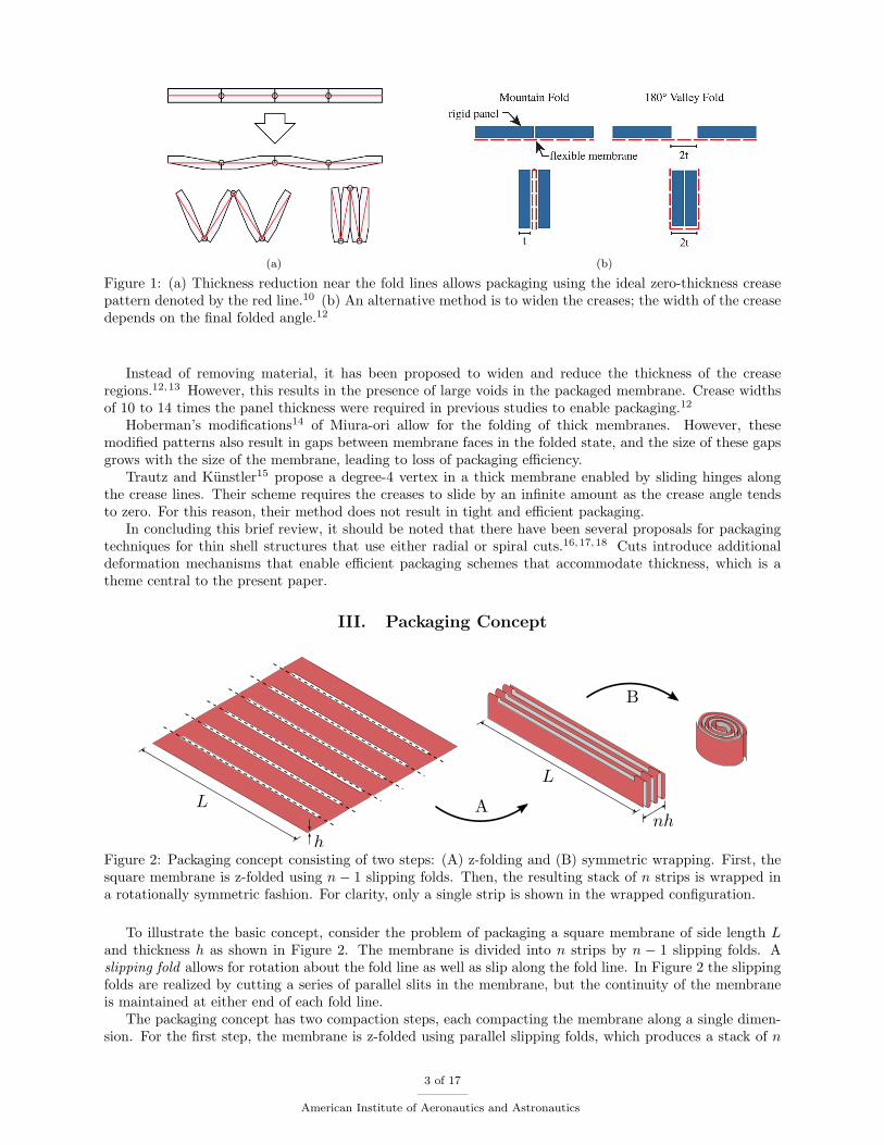
(a) (b)

Figure 1: (a) Thickness reduction near the fold lines allows packaging using the ideal zero-thickness creasepattern denoted by the red line.10 (b) An alternative method is to widen the creases; the width of the creasedepends on the final folded angle.12

Instead of removing material, it has been proposed to widen and reduce the thickness of the creaseregions.12,13 However, this results in the presence of large voids in the packaged membrane. Crease widthsof 10 to 14 times the panel thickness were required in previous studies to enable packaging.12

Hoberman’s modifications14 of Miura-ori allow for the folding of thick membranes. However, thesemodified patterns also result in gaps between membrane faces in the folded state, and the size of these gapsgrows with the size of the membrane, leading to loss of packaging efficiency.

Trautz and Kunstler15 propose a degree-4 vertex in a thick membrane enabled by sliding hinges alongthe crease lines. Their scheme requires the creases to slide by an infinite amount as the crease angle tendsto zero. For this reason, their method does not result in tight and efficient packaging.

In concluding this brief review, it should be noted that there have been several proposals for packagingtechniques for thin shell structures that use either radial or spiral cuts.16,17,18 Cuts introduce additionaldeformation mechanisms that enable efficient packaging schemes that accommodate thickness, which is atheme central to the present paper.

III. Packaging Concept

Figure 2: Packaging concept consisting of two steps: (A) z-folding and (B) symmetric wrapping. First, thesquare membrane is z-folded using n − 1 slipping folds. Then, the resulting stack of n strips is wrapped ina rotationally symmetric fashion. For clarity, only a single strip is shown in the wrapped configuration.

To illustrate the basic concept, consider the problem of packaging a square membrane of side length Land thickness h as shown in Figure 2. The membrane is divided into n strips by n − 1 slipping folds. Aslipping fold allows for rotation about the fold line as well as slip along the fold line. In Figure 2 the slippingfolds are realized by cutting a series of parallel slits in the membrane, but the continuity of the membraneis maintained at either end of each fold line.

The packaging concept has two compaction steps, each compacting the membrane along a single dimen-sion. For the first step, the membrane is z-folded using parallel slipping folds, which produces a stack of n

3 of 17


strips. For the second step, this stack of strips is wrapped in a rotationally symmetric fashion.The slipping folds are needed to accommodate the incompatibility created by wrapping the thick mem-

brane strips around different radii. The symmetric wrapping scheme ensures that the ends of the strips canremain connected. The following two subsections will explain in detail the two enabling concepts of slippingfolds and symmetric wrapping.

III.A. Slipping Folds

The proposed packaging concept relies on material removal along fold lines to create slipping folds. Themembrane can be folded and unfolded at such slipping folds without straining the material. In some sense,a slipping fold is an extreme case of a score; whereas a score weakens the membrane to localize bendingstrains, a slipping fold removes material entirely.

The two degrees of freedom of a slipping fold are shown in Figure 3. In addition to the fold angle, ρ,slipping folds have a slip degree of freedom, ξ, which is the linear displacement of the material on one sideof the fold with respect to the material on the other side, in the direction of the fold line. An ideal slippingfold has zero stiffness associated with both these degrees of freedom.

Figure 3: Slipping folds have two degrees of freedom: fold angle ρ and slip ξ.

Because material removal along the fold lines leads to a reduction in the continuity and hence in thestiffness of a structure, several realizations of slipping folds have been considered that are not simple cuts.These realizations include connections that allow for the transmission of tension forces and the limitedtransmission of shearing forces across fold lines. Figure 4 illustrates two possible methods for forming theseconnections.

Hinged fold A cylindrical rod is located at the fold line. This rod is attached to the material on one sideof the fold using tabs. The material on the other side is attached to the rod using a loop. This loopcan rotate about the rod and slip along the rod. Maximum slip is reached when the loop contacts atab. A hinged fold transmits tension across the fold line. In the maximum slip state, a shearing forcemay also be transmitted.

Ligament fold To create a ligament fold, one or more thin strips of material are left uncut at the fold line.The length of the ligament is chosen to allow for the required deformation along the fold line. Likethe hinged fold, a ligament fold has state of maximum slip beyond which the ligament will deformplastically. A ligament fold allows for the transmission of tension and shear across the fold line.

The slip degree of freedom is crucial; it enables the second compaction step of wrapping. Wrapping thez-folded stack of n strips leads to the outer strips going around larger radii than the inner strips becauseeach strip has thickness h > 0. Thus, for the same arclength, outer strips traverse smaller wrapping anglesthan inner layers. If the strips cannot slip against each other, wrapping the stack of strips will result instraining of the membrane.

In addition to areas where the membrane strips can slip against each other, it is also advantageous toconstrain the slip to be zero at certain locations, which allows the strips to be connected at the ends. Thiscondition can be achieved by using a rotationally symmetric wrapping.

III.B. Symmetric Wrapping

Symmetric wrappings are a class of wrappings that result in a configuration that has two-fold symmetry.Using these wrappings, it is possible to enforce zero slip, for example, at the two ends of the z-folded stack,which enables the edges of the membrane to remain uncut and able to transmit tension. The ability of

4 of 17


(a) Hinged fold. (b) Ligament fold.

Figure 4: Two examples of slipping folds with connections across the fold lines that still allow for the rotationand slip degrees of freedom.

the edges to transmit tension will be useful when a concept for prestressing the membrane are discussed inSection IV.

The membrane strips in the wrapped stack are modeled as a set of curves offset from a base curve. (Ifthe number of strips n is odd, the base curve corresponds to the middle strip.)

The base curve r(s) : [−L/2, L/2] ! R2 is parametrized by its arclength s. As shown in Figure 5, the

ith strip is offset from the base curve by q(i)n(s), where n(s) is the normal to the base curve and q(i) is aseparation distance. (If n is odd, q(i) = ih.) Thus the ith strip follows the offset curve r(i; s) = r(s)+q(i)n(s).

Figure 5: Offset curves separated by a normal distance q(i).

For the ends of the strips to be connected, the length of the ith strip Li must equal the length of thebase curve L for all i. This is possible when the integral of the signed curvature κ(s) of the base curve iszero. To see this, consider the formula for the length Li of the ith strip:

Li =

Z L/2

−L/2

kr0(i; s)k ds (1)

kr0(i; s)k = kr0(s) + q(i)n0(s)k (2)

Now the derivative of the normal vector n0(s) is parallel to the tangent vector r0(s) and has length |κ(s)|:19

n0(s) = −κ(s)r0(s) (3)

Substituting this into the expression for kr0(i; s)k and noting that kr0(s)k = 1 gives

kr0(i; s)k = 1− q(i)κ(s) (4)

) Li =

Z L/2

−L/2

[1− q(i)κ(s)] ds = L− q(i)

Z L/2

−L/2

κ(s) ds (5)

5 of 17


Thus, for Li = L ∀ i the following condition must be satisfied:

Z L/2

−L/2

κ(s) ds = 0 (6)

A simple way to meet this condition is to have κ(s) be an odd function of arclength, i.e. −κ(−s) = κ(s). Abase curve that has this may be defined in a piecewise manner, using a generator curve p(s) : [0, L/2] → R

2

and a copy of the generator curve rotated by 180◦:

r(s) =

8

<

:

−p(−s) if s ∈ [−L/2, 0)

p(s) if s ∈ [0, L/2](7)

For r(s) ∈ C2, p(s) ∈ C2, p(0) = 0 and p00(0) = 0 are needed.

(a) Generator curve (b) Offset curves

Figure 6: Wrapping curve for efficient packaging. The shaded areas in (b) are the only cavities that resultfrom this curve, and their size depends mainly on the minimum radius of curvature Rmin.

A generator curve that allows for compact wrapping is shown in Figure 6. It is a piecewise curve consistingof a semi-circle of radius R, a vertical line of length f , and an involute of a circle with pitch 2πf :

p(s) =

8

>

>

>

>

>

<

>

>

>

>

>

:

R {1− cos (s/R),− sin (s/R)} if s ∈ [0, πR]

R {2, (s/R)− π} if s ∈ (πR, πR+ f)

f {cos (α− θ) + α sin (α− θ),

sin (α− θ)− α cos (α− θ)}if s ∈ (πR+ f, L/2)

(8)

α2 =2

f(s− πR− f) +

✓

2R

f

◆2

(9)

θ =2R

f−

π

2(10)

Note that this particular generator curve has discontinuous curvature at all points where two pieces meet.Therefore it is not expected that a wrapped membrane will follow this curve exactly; however, it is a simplecurve that may be used to estimate the size of the packaged membrane, which will be contained within acylinder of radius Rp and height Hp.

A strip thickness multiplier φ ≥ 1 is included to account for the fact that in the packaged configurationthe strips may be separated by some distance φh ≥ h. The pitch of the involute 2πf = 2nφh accounts for

6 of 17


the thickness of the z-folded stack of strips. The radius of the semi-circle R = Rmin + φhn/2 is such thatthe curvature limit 1/Rmin, dictated by the material modulus E and yield stress σy, is not exceeded:

1

Rmin=

2σy

Eh(11)

III.C. Packaging Efficiency

The packaged radius is Rp = max kr(i; s)k and the packaged height is Hp = L/n. Using these, the packagingefficiency η, which is the ratio of the packaged volume to the material volume of the membrane, can beestimated.

η =L2h

πR2pHp

(12)

The packaging efficiency is a function for four non-dimensional parameters: n, ψ ⌘ Rmin/h, λ ⌘ L/h, andφ. It has the following expression:

η =nλ

πγ2(13)

γ2 ⌘

✓

Rp

h

◆2

= φ2

"

⇣n

π

⌘2

+⇣nαmax

π

⌘2

+

✓

n− 1

2

◆2

+n(n− 1)

παmax

#

(14)

α2max =

πλ

nφ+

2π2ψ

nφ− 2 +

✓

2πψ

nφ

◆2

(15)

Figure 7 shows the variation of the packaging efficiency with λ, ψ, and φ. The effect of n on the packagingefficiency is minimal, since as n increases, the packaged height decreases, but the packaged radius increases,and thus the packaged volume varies minimally.

λ

η

103

104

105

106

107

0

0.2

0.4

0.6

0.8

1

= 1

= 1.125

= 1.25

= 1.375

= 1.5

(a) n = 100, ψ = 50

λ

η

103

104

105

106

107

0

0.2

0.4

0.6

0.8

1

= 5

0

= 1

25

= 2

00

= 2

75

= 3

50

(b) n = 100, φ = 1

Figure 7: Packaging efficiency η as a function of the dimensionless deployed length λ = L/h, the dimensionlessminimum bend radius ψ = Rmin/h, and the strip thickness multiplier φ. For (a), n and ψ are held constant,and for (b), n and φ are held constant.

Figure 7a shows that the strip thickness multiplier φ has the greatest effect on the packaging efficiency forlarge λ. In fact, in the limit of λ ! 1, η ! 1/φ. This means that for very large or very thin membranes, theglobal packaging efficiency depends only on the local, per-strip packaging efficiency. Figure 7b shows thatthe minimum bend radius of the material Rmin = hψ has the greatest effect for small λ. As λ increases, thesize of the two cavities (which is determined by Rmin) shown in Figure 6 shrinks in relation to the membranevolume and the effect of ψ decreases.

7 of 17


IV. Prestressing Concept

A membrane with slipping folds is anisotropic; the stiffness parallel to the slipping folds is much higherthan the stiffness perpendicular to them. This anisotropy must be taken into account when prestressing themembrane. This section presents one particular solution to the problem of prestressing membranes of thistype.

Consider a membrane as shown in Figure 8a with slipping folds parallel to the y-axis, length a along thex-axis and length b along the y-axis. When prestressed, it is desired that each strip has equal tension inthe y-direction, i.e. parallel to the slipping folds, and no tension in the x-direction, i.e. perpendicular to theslipping folds.

Consider applying global tensioning forces Fx at [±a/2, 0] and Fy at [0,±b/2] (using suitable externalcompression members e.g. booms or masts); the membrane edges can be shaped such as to distribute thesetensioning forces to uniaxial tensile loading P , which is a force per unit length. Since the symmetric wrappingensures that the edges of the membrane remain continuous and uncut, they can transmit tension. It is easyto show that for P uniform, the edge profile f(x) : [0, a/2] → R must be parabolic:

(a)

b/a

Pa/2Fx

0 0.5 1 1.5 2

0

0.5

1

1.5

2

2A/ab

0.7

0.75

0.8

0.85

0.9

0.95

1

(b)

Figure 8: (a) Membrane with parabolic edges tensioned uniformly and uniaxially by four radial forces.(b) Membrane area A normalized by the rhombus area ab/2 as function of the aspect ratio b/a and thenormalized loading Pa/2Fx. The white triangle is inaccessible due to f 0(a/2) ≤ 0.

f(x) =

✓

P

Fx

◆

x2−

✓

Pa

2Fx+

b

a

◆

x+b

2(16)

The edges of the membrane can be constructed by taking f(x) and mirroring it about the x and y axes. Toensure f(x) ≥ 0, it is insisted that f 0(a/2) ≤ 0, and hence

Pa

2Fx−

b

a≤ 0 (17)

Two non-dimensional parameters, the loading parameter Pa/2Fx and the aspect ratio b/a, determinekey aspects of this structure. The membrane area A normalized by the rhombus area ab/2 is a function ofthese parameters, as is the ratio of the global tensioning forces Fy/Fx:

2A

ab= 1−

1

3

a

b

Pa

2Fx(18)

Fy

Fx=

Pa

2Fx+

b

a(19)

Figure 8b plots the dimensionless area as a function of these two parameters.

8 of 17


V. Deployment Concept

This section discusses a particular concept for deploying a slip-wrapped membrane with parabolic edges.The deployment concept, shown in Figure 9, consists of an unwrapping stage followed by an unfolding stage.

Figure 9: The two stages of deploying a slip-wrapped membrane with parabolic edges. For clarity, just onestrip is shown during the unwrapping stage.

In the unwrapping stage, the two ends B and B0 of the wrapped stack are pulled in opposite directionsby applying forces FB and FB0 . The separation b between B and B0 increases until b = b.

In the unfolding stage, the stack of strips is unfolded by applying forces FA and F 0

A at points A and A0.The separation between these points a grows to a at the end of deployment.

(a) Cage (isometric view) (b) Clip (section view)

Figure 10: Deployment restraints.

A “cage”, shown in Figure 10a, is used to manage the unwrapping process. It is a cylindrical tube withtwo slots. The endpoints B and B0 of the folded membrane stack are pulled out through these slots. Duringthe unfolding stage, the two halves of the cage must separate and move apart, see Figure 9.

A “clip”, shown in Figure 10b, holds the folded stack of the strips together at its midpoint. It managesthe unfolding stage; it ensures that when the endpoints A and A0 of the folded stack are pulled outwards, thestrips deploy one at a time. The wrapped membrane rotates with respect to the cage during the unwrappingstage, and hence the clip has to rotate as well.

An experimental implementation of this concept is presented in the following section.

9 of 17


VI. Test Apparatus and Procedures

VI.A. Packaging Tests

To wrap a membrane according to the technique described in Section III, a “wrapping plug” can be used toguide the folded membrane stack along the designed curve and prevent the membrane from exceeding themaximum curvature limit as provided by Equation (11). Figure 11a shows a conceptual plug; it consists oftwo halves shaped like the cavities in the wrapping curve of Figure 6.

(a) Conceptual design

(b) Design details

Figure 11: Wrapping plug.

A wrapping plug suitable for polyester films of thickness of up to 50.8 m was designed. AssumingE = 3.50GPa and σy = 100MPa for polyester films, Equation (11) gives Rmin of 0.89mm. However,fabrication constraints imposed an upper bound on Rmin of 2mm, and therefore there was a margin ofsafety of 2.25 against plastic deformation in the membrane. A detailed design of the wrapping plug withRmin = 2mm and a length of 45mm is shown in Figure 11b.

The two halves of the plug were fabricated from UV-curable acrylic plastic using stereolithography. Eachhalf of the plug has a lengthwise hole to accept a threaded rod. Each half also has small pegs at either endthat mate with two end plates. These end plates hold the two halves of the plug in alignment. Two threadedrods are passed through the lengthwise holes in the plugs and the end plates, and are held in place by nuts.

Two square models were made from aluminized polyester film and wrapped around this plug. Table1 lists the relevant parameters of these models. These models had ligament slipping folds made using acomputer-controlled laser cutter (Universal Laser Systemsr ILS9.75). There were 7 ligaments per fold line.The ligaments had widths of 1.5mm, lengths of 8mm, and rounded corners.

Model h ( m) L(m) log10(λ) n ψ

1 25.4 0.5 4.3 13 78.7

2 50.8 0.5 4.0 13 39.4

Table 1: Packaging models

To package the membrane, it was first folded into a stack of strips. The strips were then pre-slipped withrespect to each other at the middle of the stack by 1.1mm and 1.7mm respectively for models 1 and 2. Thispre-slip was induced before the membrane stack was inserted into the plug. When packaging without a plug,this step of pre-slipping is not required, since the strips are free to slip during packaging. However, the plugtightly clamps the strips against each other and prevents slip from developing during packaging. Therefore,it was necessary to pre-slip the strips.

The strips were then manually wrapped tightly against the plug. A loop of string was used to hold themembrane wrapped while a digital caliper was used to measure the packaged diameter at the middle of thewrap. Figure 12 shows model 2 wrapped around the plug.

10 of 17


Figure 12: Model 2 wrapped around the plug. The packaged diameter was 23.92mm.

VI.B. Prestressing Test

To demonstrate the feasibility of the prestressing concept, an aluminized polyester film model with b/a =Pa/2Fx = 1, a = 0.8m, h = 50.8 m was made. The parabolic edge and the ligament slipping folds weremade using the laser cutter. Since b/a = Pa/2Fx = 1, Fy/Fx = 2.

Figure 13 shows the model hanging on a metal-backed chalkboard using magnets. The tensioning forceswere applied by hanging weights: Fy was applied by hanging a 50 g weight and pinning the top corner ofthe membrane and Fx was applied through a pulley by hanging a 25 g weight and pinning the right cornerof the membrane.

Inspection of the model showed that each strip was in a state of tension, and that the model was ableto hang flat, though there was some residual transverse curvature of the strips from the film having beenstored on a roll.

Figure 13: Hanging model test of prestressing concept.

11 of 17


VI.C. Deployment Test

To test the deployment concept presented in Section V, a membrane model with parabolic edges and ligamentslipping folds was fabricated. The model had b/a = Pa/2Fx = 1, a = 1m, h = 25.4 m, and was made fromaluminized polyester film. Because the laser cutter allowed a maximum part size of 0.91m × 0.61m, themodel was fabricated in three separate pieces, which were joined together using polyimide tape.

The deployment rig shown in Figure 14 was used to test the deployment concept. It consisted of fourindependent linear actuators to provide the deployment forces FB , FB0 , FA, FA0 , four force sensors to recordthe deployment forces, and a suspension system to partially offload the mass of the membrane.

Each linear actuator consisted of a lead screw coupled to a stepper motor that drives a carriage backand forth along a rail. Each stepper motor is driven by a separate microstepping driver. A micrcontrollersynchronized the four motors, as well as providing logic, displacement data logging, and an interface to aPC.

Each carriage had a sensitive six-axis force sensor (ATI Industrial Automation Nano17) that measuresdeployment force with a resolution of 3.1 N.

Figure 14: Two-axis deployment rig.

Figure 15 shows the cage and the clip as fabricated. The cage was made of two laser-cut acrylic baseplates, 125 m-thick polyimide rectangular plates elastically bent into half-pipes, and threaded rods to attachthe half-pipes to the base plates. The cage was constructed in two halves, which need to separate for theunfolding stage of the deployment. The inside faces of the half-pipes were coated with a dry lubricant to

12 of 17


reduce friction between the cage and membrane during unwrapping.A clip prototype was made using two paintbrush heads (7mm × 4mm cross section, 11mm length)

connected by a steel rod. The paintbrush bristles were pushed into the middle of the wrapped membranestack. The membrane strips were spaced apart at this clip insertion point. This separation between themembrane strips ensured that they deployed one by one.

Figure 15: The cage and the clip, as fabricated. The membrane model has been wrapped and inserted intothe cage with the clip. The cage half-pipes have a diameter of 37mm and a height of 49mm.

To simulate deployment in a 0 g environment, the clip was suspended about 0.25m above the base of thetwo-axis deployment rig. Since the clip holds the middle of the membrane during most of the deployment,suspending the clip helped offload some of the weight of the membrane. A 400 g weight was suspended fromthe bottom of the clip to stabilize its orientation. The membrane weight was also partially offloaded at theattachment to the force sensors. The membrane was deployed in a horizontal plane. However, this setup isonly an approximate gravity offload scheme, and it is expected that the measured deployment forces includea component of the membrane weight.

VII. Test Results

VII.A. Packaging Test Results

The two models listed in Table 1 were packaged according to the procedure described in Section VI.A. Theirdiameters at the middle of the wrapped stack, i.e. away from the ligaments and close to the restrainingstring, were measured and used to calculate their packaging efficiencies, which are plotted in Figure 16.

Also plotted are lines of varying λ with the same n and ψ values as the models, with φ such that theselines pass through the experimental points. These lines represent packaging efficiencies achievable usingsimilar manufacturing and packaging techniques, but scaled to different λ.

VII.B. Deployment Test Results

The membrane model described in Section VI.C was deployed using the two-axis rig. The in-plane radial de-ployment forces FB , FB0 , FA, FA0 were measured, and are plotted in Figure 17 with respect to the unwrappingdeployment fraction b/b and the unfolding deployment fraction a/a. (The in-plane transverse deployment

13 of 17


λ

η

102

103

104

105

106

107

108

0

0.1

0.2

0.3

0.4

0.5

0.6

0.7

0.8

0.9

1

ϕ = 1.057

Model 1 (η= 69%)

ϕ = 1.106

Model 2 (η= 73%)

Figure 16: Packaging test results. Packaging efficiency η is plotted with respect to dimensionless deployedlength λ = L/h for the two packaging models. Also shown are the two packaging efficiency curves with thesame values for n and ψ as the packaging models, with the strip thickness multiplier φ adjusted such thatthese curves pass through the experimental points.

forces were about 20 times smaller than the radial forces, and are not shown. The out-of-plane forces areprimarily due to the weight of the membrane and are not shown.) The radial component of the deploymentforces never exceeded 0.6N. The deployment was displacement controlled at a rate of about 11.9mms−1.

During the unwrapping stage, the deployment forces were largely caused by friction between the wrappedmembrane rotating inside the cage and rubbing against the walls of the cage. Note that during the initialstages of unwrapping, FB0 ! FB . This is because pulling on one end of the wrapped stack causes the otherend to deploy; in a displacement-controlled deployment any lag between the two ends of the wrapped stackis persistent.

During the unfolding stage, the deployment forces FA and FA0 show a snapping behavior as each strip isdeployed from the clip. The separation of these snaps indicates the separate (as opposed to simultaneous)unfolding of each strip. Indeed, that is what was observed: each strip was deployed separately and insequence.

Figure 18 shows views from an overhead camera at the beginning of deployment, at the end of theunwrapping stage, during the unfolding stage, and at the end of the deployment.

14 of 17


Fo

rce

(N

)

0 0.2 0.4 0.6 0.8 1 0.2 0.4 0.6 0.8 1-0.1

0

0.1

0.2

0.3

0.4

0.5

FB

FB′

FA

FA′

ā/ab/b

Figure 17: Deployment force profiles. b/b is the unwrapping deployment fraction and a/a is the unfoldingdeployment fraction. During the first stage of unwrapping, the unfolding deployment fraction a/a is fixedat 0, and during the second stage of unfolding, the unwrapping deployment fraction b/b is fixed at 1.

15 of 17


(a) Packaged (b) Unwrapped

(c) Unfolding (d) Deployed

Figure 18: Deployment test for a membrane with a = b = 1m, h = 25 m viewed from an overhead camera.

16 of 17


VIII. Conclusion

A scheme for packaging thick membranes is presented that compacts the membrane along two dimensionsby first folding and then wrapping the membrane. This scheme allows the membrane to be packaged tightly,with very few voids, and without plastic creases. Slipping folds are used to accommodate material thickness.

These slipping folds rely on material removal; however, realizations of slipping folds are described thatallow for the transmission of tension forces across the fold lines. A two-fold symmetric wrapping scheme isdescribed that allows for the preservation of continuity at the edges of the membrane.

A kinematic model for the wrapped membrane is used to estimate packaging efficiencies, which approaches100% for tightly wrapped membranes with large length-to-thickness ratios. Packaging tests on 0.5m-scalemodels achieved packaging efficiencies of 69% and 73%.

Also presented is a strategy for prestressing a membrane packaged using slipping folds. This strategyuses the continuous edges of the membrane to distribute radial prestress forces into uniform tension parallelto the fold lines. A 0.8m-scale prototype was used to demonstrate the feasibility of this prestressing strategy.

A two-stage method for deploying a slip-wrapped membrane is proposed. Initial tests conducted on1m-scale models showed successful and controlled deployment with low unfolding forces.

Acknowledgments

Support from the Northrop Grumman Corporation is gratefully acknowledged.N. Lee was supported through this work by a postdoctoral fellowship from the W. M. Keck Institute for

Space Studies.

References

1Miura, K., “Method of packaging and deployment of large membranes in space,” Proceedings of the 31st Congress of theInternational Astronautical Federation IAF-80-A 31 Tokyo, pp. 1–10, 1980.

2Miura, K. and Natori, M. “2-D array experiment on board a space flyer unit,” Space Solar Power Review, vol. 5, pp.345–356, 1985.

3Biddy, C. and Svitek, T., “LightSail-1 Solar Sail Design and Qualification,” 41st Aerospace Mechanisms Symposium,2012, pp. 451–463.

4Montgomery, E. E. I. and Adams, C. L., “NanoSail-D,” CubeSat Developer’s Workshop, 2008.5Furuya, H., Mori, O., Okuizumi, N., Shirasawa, Y., Natori, M. C., Miyazaki, Y., and Matunaga, S., “Manufacturing

and Folding of Solar Sail IKAROS,” 52nd AIAA/ASME/ASCE/AHS/ASC Structures, Structural Dynamics, and MaterialsConference, Apr. 2011.

6Lee, N. and Close, S., “Curved pleat folding for smooth wrapping,” Proceedings of the Royal Society A: Mathematical,Physical and Engineering Sciences, vol. 469, issue 2155, 2013.

7Satou, Y. and Furuya, H., “Fold Line Based on Mechanical Properties of Crease in Wrapping Fold Membrane,” 54thAIAA/ASME/ASCE/AHS/ASC Structures, Structural Dynamics, and Materials Conference, Apr. 2013.

8Murphey, T. W., A nonlinear elastic constitutive model for wrinkled thin films, Ph.D. thesis, 2000.9Papa, A. and Pellegrino, S., “Systematically Creased Thin-Film Membrane Structures”, Journal of Spacecraft and Rock-

ets, Vol. 45, No. 1, 2008, pp. 10-18.10Tachi, T., “Rigid-Foldable Thick Origami,” Origami 5 , edited by M. Yim, 2011, pp. 253–263.11Guest, S. D. and Pellegrino, S., “Inextensional wrapping of flat membranes,” First International Seminar on Structural

Morphology, Sept. 1992, pp. 203–215.12Zirbel, S. A., Lang, R. J., Thomson, M. W., Sigel, D. A., Walkemeyer, P. E., Trease, B. P., Magleby, S. P., and Howell,

L. L., “Accommodating Thickness in Origami-Based Deployable Arrays,” Journal of Mechanical Design, Vol. 135, Nov. 2013,pp. 111005.

13Reynolds, W. D. and Murphey, T. W., “Elastic Spiral Folding for Flat Membrane Apertures,” 55thAIAA/ASME/ASCE/AHS/ASC Structures, Structural Dynamics, and Materials Conference, Jan. 2014.

14Hoberman, C., “Reversibly Expandable Structures,” United States Patent No. 4,981,732, 1991.15Trautz, M. and Kunstler, A., “Deployable folded plate structures folding patterns based on 4-fold-mechanism using stiff

plates,” Proceedings of the International Association for Shell and Spatial Structures Symposium, pp. 2306–2317, Oct. 2009.16Greschik, G., “Deployment of Dishes with Surface Discontinuities,” Journal of Spacecraft and Rockets, Vol. 33, No. 4,

1996.17Tibbalds, B., Guest, S. D., and Pellegrino, S., “Inextensional Packaging of Thin Shell Slit Reflectors,” Technische

Mechanik , Vol. 24, No. 3-4, 2004, pp. 211–220.18Reynolds, W. D., Murphey, T. W., and Banik, J. A., “Highly Compact Wrapped-Gore Deployable Reflector,” 52nd

AIAA/ASME/ASCE/AHS/ASC Structures, Structural Dynamics, and Materials Conference, Apr. 2011.19Spivak, M., A Comprehensive Introduction to Differential Geometry, Vol. II, 3rd ed., 1999.

17 of 17


Documents

W. M. Keck Institute for Space Studies Postdoctoral ...kiss.caltech.edu/papers/reports/nicolas-lee-final-report.pdf · Postdoctoral Fellowship Final Report Nicolas Lee ... (2014),