Embed Size (px)
Citation preview
HAL Id: tel-01024471https://tel.archives-ouvertes.fr/tel-01024471
Submitted on 16 Jul 2014
HAL is a multi-disciplinary open accessarchive for the deposit and dissemination of sci-entific research documents, whether they are pub-lished or not. The documents may come fromteaching and research institutions in France orabroad, or from public or private research centers.
L’archive ouverte pluridisciplinaire HAL, estdestinée au dépôt et à la diffusion de documentsscientifiques de niveau recherche, publiés ou non,émanant des établissements d’enseignement et derecherche français ou étrangers, des laboratoirespublics ou privés.
Vulnérabilité, Interdépendance et Analyse des Risquesdes Postes Sources et des Modes d’Exploitation
décentralises des Réseaux ElectriquesJosé Libardo Sanchez Torres
To cite this version:José Libardo Sanchez Torres. Vulnérabilité, Interdépendance et Analyse des Risques des PostesSources et des Modes d’Exploitation décentralises des Réseaux Electriques. Sciences de l’ingénieur[physics]. Université de Grenoble, 2013. Français. <tel-01024471>
Université Joseph Fourier / Université Pierre Mendès France / Université Stendhal / Université de Savoie / Grenoble INP
THÈSE Pour obtenir le grade de
DOCTEUR DE L’UNIVERSITÉ DE GRENOBLE Spécialité : Génie Electrique Arrêté ministériel : 7 août 2006
Présentée par
José Libardo / SANCHEZ TORRES Thèse dirigée par Nouredine/HADJSAID et Co-encadré par Raphaël/CAIRE préparée au sein du Laboratoire G2ELAB dans l'École Doctorale Electronique, Electrotechnique, Automatique, Télécommunication et Traitement du Signal
Vulnérabilité, Interdépendance et Analyse des Risques des Postes Sources et des Modes d’Exploitation décentralises des Réseaux Electriques
Thèse soutenue publiquement le 23 Octobre 2013, devant le jury composé de : M. Jovica MILANOVIC Professeur à l’Université de Manchester, Président M. Abdellatif MIRAOUI Professeur à l’Université Cadi Ayyad, Rapporteur M. Nouredine HADJ SAID Professeur à Grenoble INP, Directeur de thèse
M. Raphaël CAIRE Maître de Conférences de Grenoble INP, Co-encadrant M. Olivier HUET Head of Strategy ERDF, Examinateur


This dissertation is dedicated to my family, my dad Libardo, my mom Marcela,
my sister Paloma, my little brother Rodrigo and my better half Marianita.
CARPE DIEM


ACKNOWLEDGMENTS
“Gracias a la vida, que me ha dado tanto, me ha dado el sonido y el abecedario, con él, las pa-
labras que pienso y declaro: Madre, amigo, hermano y luz alumbrando, la ruta del alma de la que estoy amando” – Mercedes Sosa
3 years, 4 summers, 3 winters, 1218 days, 174 weeks… it is a long time, isn’t it? It is not possi-ble to succeed alone in research for a long time; discussions, movies, people, news and friends inspire and new ideas born. Thus many people were involved either directly or indirectly on this dissertation. Even many people might not understand why I would like to thank them. I believe that if we live without thinking about rewards and we just do what we feel, from the heart, we will maximize the happiness in the world, we will not be worried about little things and we will enjoy the fact that we are alive and that we can help other people. For this reason, it is a pleasure for me to thank those who made this thesis possible.
Firstly, I would like to thank Mr. Jovica Milanovic, Mr. Abdelatif Miraoui and Mr. Olivier Huet for their general interest, their feedbacks and their comments and for proofreading the manuscript. It is an honor for me to have a great evaluators committee with many years of experience.
Further, I am grateful to Mr. Nouredine Hadjsaid and Mr. Raphael Caire. Firstly, because they proposed me a fascinating research subject with a great sponsor, and secondly because they guided me and trusted my work and ideas.
I would like to show my gratitude to the SINARI Project members, for the stimulating discus-sions, for their support and for presenting me different research domains.
I owe my deepest gratitude to Mr. Mario Rios, who motivated me during my first steps in the electrical engineering at Universidad de los Andes and proposed me an interesting project for my Mas-ter degree. Afterwards, he encouraged me to pursuit a PhD Degree at G2ELAB. I must say that with-out his motivation and encouragement, I would not have had the opportunity to come to France and to acknowledge the enjoyable and passionate Research World.
Research without documentation, papers, books and other resources is not possible. I would like to thank Mme. Sylvie Garcia, for her work and for letting me win the G2ELAB Petanque Tournament 2013 (well, it was a team work, thanks Ando and Daniel). As well as Elise, who helped me for the work-travel planning and was so patient with me.
When I arrived to Grenoble, I had a very limited French-speaking level. But it was not an obsta-cle to find welcoming people, Asma, Lina, MC, Olivier, Yann, Jérémie, Phuong and Damien. I re-member lunchtime with all of them at the office D-060 when I couldn’t understand a single phrase.

They introduce me the lab, the coffee time, but since they were 3rd year (almost 4th), they started leaving the laboratory.
Then, I found an already formed group from the Master program at ENSE3 and the fresh 1st year students. I would like to thank Camille for the enjoyable conversations. Mihn, Ni, Kaustav, Ando, Luiz, Lyuvo, Selle, Long, Mathieu, Archie and other colleges, all of them were part of my process to become a PhD, who is not only a person that knows a lot about a single subject, but a person with the maturity of an adult to identify complex problems and with the curiosity of a child to try new and orig-inal solutions.
During my second year I was getting crazy and I started dreaming with networks. Yes ! Mr. Ba-rabasi was right: “Networks are everywhere.” So, I found a supporting group and a new passion: The Fish-keeping. The AASG Club (Association Aquariophile Sud-Grenoblois), with his president Mr. Fred Salmeron and the other members: Denis, Mario, Marc, Carine, Fred 2, André, Udo, Julien,… they offered me a place to connect with nature, to study other sciences and to share experiences in a “Not-secret” French Society. Thanks to all of them!
My family at the lab is complete with my lab mates: Nathalie, Raha and Julian. We share many coffee times, Frisbee times, BBQ’s, Birthdays… thanks for their support and for being there.
Many other friends helped me in the distance. Juan Rozo, he knew how to motivate me. Carlos Rodriguez guided me in the difficult path of living abroad. Camilo (Conejo), Dianis, Carlitos and Juan Carlos were there every time I went back to Colombia to show me their support and to encourage me. Thanks a lot!
Also, there are four people, living in South America, far far away in a country called Colombia, they always believed in me. Two of them, my parents, they put a t-shirt on me when I was a baby say-ing “I will be a Scientist,” so the less I can do is to get a PhD diplome. The other two, my sister and my brother, they are always ready to support me even if my decisions take me 8800km away from them. I have to thank life, for putting me in this family. For that reason, it is an honor to dedicate all this work to them; they deserve the best of the best.
Finally, 3-years have passed, with a lot of study, hard work, smiles, laughs, tears and it is diffi-cult to overcome all without a better half, a soul mate, una media naranja, or call it as you like. I found between books, graphs, papers, computers, kites and numbers a person that is my best friend, my best travel partner, the best dancer, the best singer, the best cook and my future wife. I found a person that is willing to be at my side, to fight for our dreams, to solve the complex life problems, to explore the unexplored, to take decisions from the heart and to accept me even if I have 9-aquariums at home!!! Merci Mariamty!
CONTENTS
L IST OF FIGURES ........................................................................................................................... I
L IST OF TABLES ........................................................................................................................... V
L IST OF ACRONYMS .................................................................................................................. VII
L IST OF NOTATIONS ................................................................................................................... IX
GENERAL INTRODUCTION ........................................................................................................... 1
CHAPTER I CONTEXT AND DEFINITIONS ............................................................................. 5
I.1 INTRODUCTION ................................................................................................................ 6
I.2 CRITICAL INFRASTRUCTURES (CIS) ................................................................................ 8
I.2.1 Definitions ............................................................................................................ 8
I.2.2 Types of Interdependencies .................................................................................. 9
I.2.3 Types of Failures ................................................................................................ 10
I.3 ELECTRIC POWER SYSTEMS (EPS) ................................................................................ 11
I.3.1 Structure of Electric Power Systems .................................................................. 11
I.3.2 The Liberalized World and the Distributed Generation (DG) ............................ 13
I.4 ICTS FOR POWER SYSTEMS ........................................................................................... 14
I.4.1 Control assets of EPS ......................................................................................... 14
I.4.1.1 Remote Terminal Units (RTUs) .......................................................... 14
I.4.1.2 Programmable Logic Controllers (PLCs) ........................................... 15
I.4.1.3 Intelligent Electronic Devices (IEDs) ................................................. 15
I.4.1.4 Supervisory Control and Data Acquisition (SCADA) ........................ 15
I.4.2 Automation of Electric Power Systems .............................................................. 15
I.5 ICT AND EPS INTERDEPENDENCIES .............................................................................. 18
I.5.1 ICT Threats on Power Systems .......................................................................... 18
I.5.2 Power System threats on ICT ............................................................................. 21
I.6 SUMMARY ...................................................................................................................... 22
CHAPTER II MODELING CRITICAL INFRASTRUCTURES: STATE -OF-THE-ART ................ 25
II.1 INTRODUCTION .............................................................................................................. 26
II.2 COMPLEX NETWORKS ................................................................................................... 27
II.2.1 Initiating event and cascade-safe operating margins ......................................... 27
II.2.2 Global vulnerability of interdependent infrastructures ..................................... 27
II.2.3 Interdependent technical infrastructures modeling ........................................... 28
II.2.4 Rule-based complex networks .......................................................................... 29
II.2.5 Advantages – Disadvantages ............................................................................. 29
II.3 AGENT-BASED MODEL (ABM) ..................................................................................... 30
II.3.1 Object-Oriented Hybrid Modeling Approach ................................................... 31
II.3.2 Agent-based input-output interdependency model ........................................... 32
II.3.3 Federated Agent-Based model .......................................................................... 32
II.3.4 Advantages - Disadvantages ............................................................................. 33
II.4 BAYESIAN NETWORKS (BN).......................................................................................... 34
II.4.1 Cause-Effect interdependencies ........................................................................ 34
II.4.2 Dynamic Bayesian Networks ............................................................................ 35
II.4.3 Advantages - Disadvantages ............................................................................. 36
II.5 BOOLEAN LOGIC DRIVEN MARKOV PROCESSES ........................................................... 36
II.6 COMBINED SIMULATORS ............................................................................................... 37
II.6.1 Cosimulator for Transport and Distribution systems ........................................ 37
II.6.2 Real-time Cosimulator ...................................................................................... 38
II.6.3 Federate-based Simulator .................................................................................. 39
II.6.4 Agent-based simulation tool: EPOCHS ............................................................ 40
II.6.5 Advantages - Disadvantages ............................................................................. 41
II.7 PETRI NETWORKS (PN) ................................................................................................. 41
II.7.1 Attack/Defense modeling .................................................................................. 42
II.7.2 “High-level” and “Low-level” Petri Nets.......................................................... 43
II.7.3 SWN and SAN integration ................................................................................ 43
II.7.4 Intrusion detection on Cyber Physical Systems ................................................ 44
II.7.5 Advantages - Disadvantages ............................................................................. 44
II.8 COMPARISON AND CONCLUSION ................................................................................... 44
CHAPTER III VULNERABILITY AND INTERDEPENDENCIES: MODELING ......................... 47
III.1 INTRODUCTION .............................................................................................................. 48
III.2 FROM GRAPH THEORY TO COMPLEX NETWORKS ......................................................... 49
III.3 CONCEPTUAL AND THEORETICAL FRAMEWORK ........................................................... 53
III.3.1 Notations of Complex Networks ..................................................................... 53
III.3.1.1 Adjacency Matrix ............................................................................. 53
III.3.1.2 Weight Matrix .................................................................................. 54
III.3.1.3 Path length, Geodesic and Diameter................................................. 54
III.3.1.4 Node Degree ..................................................................................... 55
III.3.1.5 Betweenness Centrality .................................................................... 55
III.3.1.6 Efficiency ......................................................................................... 57
III.3.2 Eigenspectral Analysis ..................................................................................... 58
III.3.2.1 Spectral Analysis .............................................................................. 58
III.3.2.2 Hilbert Space .................................................................................... 59
III.3.2.3 Hermitian Matrices ........................................................................... 60
III.4 VULNERABILITY AND CRITICALITY ANALYSIS .............................................................. 61
III.4.1 Electricity infrastructure topology analysis ..................................................... 61
III.4.2 The topology-driven Approach ........................................................................ 67
III.4.2.1 Complex-valued Node Degree ......................................................... 68
III.4.2.2 Betweenness Centrality for multi-infrastructures ............................. 69
III.4.2.3 Electrical and ICT Efficiency ........................................................... 70
III.4.2.4 Partial Conclusions ........................................................................... 71
III.4.3 Eigenspectral Analysis ..................................................................................... 72
III.4.3.1 Complex-weighted Adjacency Matrix.............................................. 72
III.4.3.2 Complex-valued node degree ........................................................... 73
III.4.3.3 Eigenspectral Centrality ................................................................... 73
III.5 SUMMARY ...................................................................................................................... 75
CHAPTER IV VULNERABILITY AND INTERDEPENDENCIES: APPLICATION ..................... 77
IV.1 TEST SYSTEM ................................................................................................................. 78
IV.2 TOPOLOGICAL APPROACH RESULTS.............................................................................. 79
IV.2.1 Adjacency Matrix ............................................................................................ 80
IV.2.2 Complex-valued Node Degree ........................................................................ 81
IV.2.3 Betweenness Centrality Analysis .................................................................... 86
IV.2.4 Efficiency ........................................................................................................ 88
IV.2.5 Results Analysis .............................................................................................. 90
IV.3 EIGENSPECTRAL APPROACH RESULTS .......................................................................... 93
IV.3.1 Complex-valued Node Degree ........................................................................ 94
IV.3.2 Prestige Analysis ............................................................................................. 95
IV.4 CONCLUSIONS ................................................................................................................ 98
CHAPTER V SYSTEM-OF-SYSTEMS VISION OF COUPLED INFRASTRUCTURES ................ 99
V.1 INTRODUCTION ............................................................................................................ 100
V.2 “LOW-LEVEL” SYSTEM DESCRIPTION ANALYSIS ........................................................ 101
V.2.1 Test system – HV/MV Substation .................................................................. 101
V.2.2 Complex-networks modeling methodology .................................................... 104
V.2.3 Results “Low level” description ..................................................................... 105
V.3 INTEGRATION OF “LOW LEVEL” AND “HIGH LEVEL” SYSTEM DESCRIPTION............... 107
V.3.1 Methodology ................................................................................................... 107
V.3.2 Test case .......................................................................................................... 108
V.4 SMART-GRIDS: A SGAM-BASED SYSTEM-OF-SYSTEMS VISION ................................. 112
V.4.1 Smart Grid Architecture Model (SGAM) ...................................................... 112
V.4.1.1 SGAM: Domains ............................................................................. 113
V.4.1.2 SGAM: Zones .................................................................................. 113
V.4.1.3 SGAM: Interoperability Layers ....................................................... 113
V.4.1.4 SGAM: Architecture ........................................................................ 114
V.4.2 Complex Networks modeling ......................................................................... 114
V.4.2.1 Step 1: High level system Description............................................. 114
V.4.2.2 Step 2: Low Level system Description ............................................ 114
V.4.2.3 Step 3: SoS vision of Smart Grids. .................................................. 115
V.5 SUMMARY .................................................................................................................... 115
GENERAL CONCLUSIONS ......................................................................................................... 117
RESUME EN FRANÇAIS ............................................................................................................. 121
1. INTRODUCTION GENERALE ................................................................................................. 122
2. VERROUS SCIENTIFIQUES .................................................................................................... 124
2.1. INTERDEPENDANCES CYBER-PHYSIQUES .................................................................... 124
2.2. MANQUE DES METHODES DE MODELISATION .............................................................. 124
2.3. INFRASTRUCTURES HETEROGENES .............................................................................. 127
3. PROJET SINARI ................................................................................................................... 127
4. OBJECTIFS DE LA THESE ...................................................................................................... 127
5. LA SOLUTION PROPOSEE ..................................................................................................... 128
6. METHODOLOGIE .................................................................................................................. 128
6.1. CONCEPTS DE BASE DES RESEAUX COMPLEXES ......................................................... 129
6.2. APPROCHE TOPOLOGIQUE ........................................................................................... 132
6.2.1. Degré des Nœuds ............................................................................................ 133
6.2.2. Betweenness Centrality ................................................................................... 133
6.2.3. L’efficacité ...................................................................................................... 134
6.2.4. Système de Test .............................................................................................. 135
6.2.1. Les résultats principaux .................................................................................. 138
6.3. L’APPROCHE SPECTRALE ............................................................................................. 142
6.3.1. Le degré complexe des Nœuds ....................................................................... 142
6.3.2. La centralité spectrale ..................................................................................... 143
6.3.3. Les résultats principaux .................................................................................. 143
6.4. DESCRIPTION « LOW LEVEL » ....................................................................................... 146
6.5. VISION GLOBALE DU SYSTEME .................................................................................... 149
7. CONCLUSIONS ET PERSPECTIVES ......................................................................................... 150
BIBLIOGRAPHY ........................................................................................................................ 151
APPENDIX A COMPLEX NETWORKS : ALGORITHMS AND APPLICATION .......................... - 1 -
A.1. TOOLBOX DEFINITION .................................................................................................. - 1 -
A.2. CENTRALITY INDEXES ................................................................................................. - 4 -
A.3. MORE INFORMATION ................................................................................................... - 6 -
A.4. BIBLIOGRAPHY ............................................................................................................ - 6 -
APPENDIX B RECENT ATTACKS AND ICT S FAILURES ........................................................ - 7 -
B.1. RECENT ATTACKS AGAINST INDUSTRIAL CONTROL SYSTEMS .................................... - 7 -
B.2. INFORMATION AND COMMUNICATION SYSTEM FAILURES LEADING TO BLACKOUTS - 10 -

B.3. CONCLUSIONS ............................................................................................................ - 11 -
B.4. BIBLIOGRAPHY .......................................................................................................... - 11 -
APPENDIX C PROJECTS INCLUDING COUPLED INFRASTRUCTURES .................................... - 15 -
C.1. PROJECTS ................................................................................................................... - 15 -
C.2. STANDARDS ............................................................................................................... - 17 -
C.3. BIBLIOGRAPHY .......................................................................................................... - 18 -
APPENDIX D PUBLICATIONS ................................................................................................. - 21 -

i
LIST OF FIGURES
Figure I:1 Distribution Domain (NIST 2012) ............................................................................... 7
Figure I:2 Dimensions of CIs interdependencies (Rinaldi, Peerenboom and Kelly 2001) .......... 9
Figure I:3 Typical structure of Electric Power Systems ............................................................. 12
Figure I:4 New Electric Power System ....................................................................................... 13
Figure I:5 Hierarchical conceptual levels of EPS (Tranchita, Hadjsaid, et al. 2010) .................. 16
Figure I:6 Electric power system and Control Network ............................................................. 17
Figure I:7 Incidents by Sector – 198 Total in Fiscal Year 2012 (ICS-CERT 2012) ................... 20
Figure I:8 Auxiliary systems power supply ................................................................................ 21
Figure II:1 Tested topological system (Zio and Sansavini 2011) ............................................... 27
Figure II:2 Power Grid and Water Network in China (Wang, Hong and Chen 2012) ................ 28
Figure II:3 Infrastructures Interdependencies (Johansson and Hassel 2010) .............................. 28
Figure II:4 Interdependencies Complex Network (B. Rozel 2009) ............................................ 29
Figure II:5 Overall SCADA model (Nan, Eusgeld and Kröger 2013) ........................................ 31
Figure II:6 Overall Dynamic Bayesian Network (Di Giorgio and Liberati 2012) ...................... 35
Figure II:7 BDMP Representation (Bouisson n.d.) ..................................................................... 36
Figure II:8 Combined Simulator (Rozel, et al. 2008) ................................................................. 37
Figure II:9 Cosimulator Architecture .......................................................................................... 38
Figure II:10 Cyber-physical power system architecture (Stefanov and Liu 2012) ..................... 39
Figure II:11 Hybrid simulator components (Müller, et al. 2012) ................................................ 40
Figure II:12 EPOCHS components (Hopkinson, et al. 2006) ..................................................... 40
Figure II:13 Petri Net Representation ......................................................................................... 41
Figure II:14 Cyber-net of Substation (Ten, Liu and Manimaran 2008) ...................................... 42
Figure II:15 “Hierarchical” Petri Nets (Chen, Sanchez Aarnoutse and Buford 2011) ............... 43 Figure II:16 Methods comparison ............................................................................................... 45
Figure III:1The 7 bridges of Königsberg .................................................................................... 49
Figure III:2From Graph Theory to Complex Networks vs. Computers Timeline ...................... 50
Figure III:3 Robustness of Random and Scale Free Networks (Barabási and Bonabeu 2003) ... 52
Figure III:4 Demonstration graphs .............................................................................................. 53
Figure III:5 Undirected and Directed graphs .............................................................................. 54
Figure III:6 Betweenness Centrality example ............................................................................. 56
Figure III:7 Efficiency assessment methodology ........................................................................ 57
Figure III:8 Efficiency for the test System .................................................................................. 58
Figure III:9 G2ELAB 14-Bus Graph .......................................................................................... 62
Figure III:10 G2ELAB 14-Bus System ....................................................................................... 62
ii
Figure III:11 IEEE 14-Bus Graph ............................................................................................... 62
Figure III:12 IEEE 14-Bus System ............................................................................................. 62
Figure III:13 IEEE 9-Bus Graph ................................................................................................. 63
Figure III:14 IEEE 9-Bus System ............................................................................................... 63
Figure III:15 IEEE 24-Bus Graph ............................................................................................... 63
Figure III:16 IEEE 24-Bus System ............................................................................................. 63
Figure III:17 IEEE 39-Bus Graph ............................................................................................... 64
Figure III:18 IEEE 39-Bus System ............................................................................................. 64
Figure III:19 IEEE 118-Bus Graph ............................................................................................. 65
Figure III:20 IEEE 118-Bus System ........................................................................................... 65
Figure III:21 Nodes Degree Distribution, IEEE 118-bus ............................................................ 66
Figure III:22 Test system ............................................................................................................ 68
Figure III:23 Demonstration graph ............................................................................................. 70
Figure III:24 Four-layer analysis ................................................................................................ 72
Figure III:25 Demonstration graph for Spectral Analysis ........................................................... 73
Figure IV:1 Complete 14-Bus Tests System ............................................................................... 78
Figure IV:2 Undirected Graph for the 14-bus Test system ......................................................... 79
Figure IV:3 Directed Graph for the 14-bus Test system ............................................................. 79
Figure IV:4 Adjacency Matrix – Undirected Network ............................................................... 80
Figure IV:5 Adjacency Matrix – Directed Network ................................................................... 80
Figure IV:6 Probability Degree Distribution .............................................................................. 82
Figure IV:7 Cumulative Degree Distribution.............................................................................. 82
Figure IV:8 Multiple infrastructure Degree distribution ............................................................. 82
Figure IV:9 Probability Distribution – IN Degree ...................................................................... 84
Figure IV:10 Cumulative Distribution – IN Degree ................................................................... 84
Figure IV:11 Multi-infrastructure Distribution – IN Degree ...................................................... 84
Figure IV:12 Probability Distribution – OUT Degree ................................................................ 85
Figure IV:13 Cumulative Distribution – OUT Degree ............................................................... 85
Figure IV:14 Multi-infrastructure Distribution – OUT Degree .................................................. 85
Figure IV:15 Edges Betweenness Centrality – Undirected Graph .............................................. 87
Figure IV:16 Edge Betweenness Centrality – Directed Graph ................................................... 87
Figure IV:17 Vertex Electric Efficiency ..................................................................................... 89
Figure IV:18 Vertex ICT Efficiency ........................................................................................... 89
Figure IV:19 Edges Electric Efficiency ...................................................................................... 92
Figure IV:20 Edges ICT Efficiency ............................................................................................ 92
Figure IV:21 Two layers graph ................................................................................................... 93
Figure IV:22 Eigenspectrum of the Electric connections matrix ................................................ 95
Figure IV:23 Eigenspectrum of the ICT connections matrix ...................................................... 95
Figure V:1”Low Level” & “High Level” description ............................................................... 101
Figure V:2 Complete 14-Bus Tests System .............................................................................. 102
Figure V:3 Substation diagram including Control devices ....................................................... 102
Figure V:4 Substation Communication Network ...................................................................... 103
Figure V:5 Auxiliary Control supply system ............................................................................ 103
Figure V:6 Substation graph ..................................................................................................... 104
Figure V:7 Integration of “Low level” and “High level” description ....................................... 107
Figure V:8 Methodology to elaborate the SoS Model .............................................................. 108
Figure V:9 Graph Electric Interdependencies Global model .................................................... 109
iii
Figure V:10 Graph ICT Interdependencies Global model ........................................................ 110
Figure V:11 SGAM Framework (CEN-CENELEC-ETSI 2012) .............................................. 112
Figure V:12 Smart Grid “High level” description .................................................................... 115
Chapitre en Français
Figure F - 1 Incidents par Secteur – 198 Total Année Fiscale 2012 (ICS-CERT 2012) ........... 123
Figure F - 2 Timeline réseaux complexes.................................................................................. 130
Figure F - 3 Degré du nœud vs. Betweenness Centrality .......................................................... 131
Figure F - 4 Types d’interdépendances ..................................................................................... 132
Figure F - 5 Système de test 14-Bus ....................................................................................... 136
Figure F - 6 Plateforme PREDIS – G2ELAB ......................................................................... 136
Figure F - 7 Graphe non-orienté pour le système 14 nœuds ................................................... 137
Figure F - 8 Graphe orienté pour le système 14 nœuds .......................................................... 137
Figure F - 9 Matrice d’adjacence réseau orienté ...................................................................... 138
Figure F - 10 In-degree du nœud réseau orienté ...................................................................... 139
Figure F - 11 Out-degree du nœud réseau orienté .................................................................... 139
Figure F - 12 Betweenness Centrality des lignes réseau orienté .............................................. 140
Figure F - 13 Efficacité des nœuds .......................................................................................... 141
Figure F - 14 Efficacité des lignes ........................................................................................... 141
Figure F - 15 Analyse multi-couche ........................................................................................ 142
Figure F - 16 Analyse multi-couche du système de Test ........................................................ 144
Figure F - 17 Poste source type ............................................................................................... 146
Figure F - 18 Réseau de communication poste source ............................................................ 147
Figure F - 19 Système d’alimentation électrique services auxiliaires ..................................... 147
Figure F - 20 Analyse multi-couche du système de Test ........................................................ 148
Figure F - 21 Vision Globale du système ................................................................................ 149

v
LIST OF TABLES
Table I:1 Critical Infrastructure Sectors in the United States ....................................................... 9
Table I:2 Events categorized by initiating and affected sector (# of events) (Luiijf, et al. 2009) 11 Table I:3 Voltage levels in France according to NF C15-11 and NF C13-200 ........................... 12
Table I:4 Longest blackouts ........................................................................................................ 22
Table III:1 Node degrees undirected graph ................................................................................. 55
Table III:2 Node degrees directed graph ..................................................................................... 55
Table III:3 Node Betweenness Centrality ................................................................................... 56
Table III:4 Edge Betweenness Centrality.................................................................................... 56
Table III:5 Graph properties for several systems ........................................................................ 61
Table III:6 Graph properties ........................................................................................................ 66
Table III:7 Node out-degree ........................................................................................................ 69
Table III:8 Node out-degree ........................................................................................................ 69
Table III:9 Betweenness Centrality Results ................................................................................ 70
Table III:10 Efficiency Results ................................................................................................... 71
Table III:11 Complex-valued node degree.................................................................................. 73
Table III:12 Demonstration graph eigenvectors .......................................................................... 75
Table IV:1 Node Degree – Undirected Graph ............................................................................ 81
Table IV:2 Node Degree – Directed Graph ................................................................................ 83
Table IV:3 Node Betweenness Centrality – Undirected and Directed Graph ............................. 86
Table IV:4 Vertices efficiency Undirected and Directed Graph ................................................. 88
Table IV:5 Edges Electric Efficiency – Undirected and Directed Graphs .................................. 90
Table IV:6 Edges ICT Efficiency – Undirected and Directed Graphs ........................................ 91
Table IV:7 Complex-Valued Node Degree ................................................................................. 94
Table IV:8 Highest Eigenvalues Electric System ....................................................................... 96
Table IV:9 Highest Eigenvalues ICT System ............................................................................. 97
Table V:1 Eigenanalisis Substation System - Ae ....................................................................... 105
Table V:2 Eigenanalisis Substation System - Ac ....................................................................... 106
Table V:3 Nodes correspondence between “High level” and “Low Level” ............................. 108
Table V:4 Results Eigenspectrum Electric Interdependencies .................................................. 111
Table V:5 Results Eigenspectrum ICT Interdependencies........................................................ 111

vii
LIST OF ACRONYMS
ABM Agent-Based Modeling
AC Alternating Current
AGC Automatic Generation Control
AMI Advanced Metering Infrastructures
ANR Agence Nationale de la Recherche
ANSSI Agence Nationale de la Sécurité des Systèmes d’Information
BN Bayesian Network
BDMP Boolean logic Driven Markov Process
BMS Business Management System
CI Critical Infrastructure
CN Complex Network
CT Current Transformer
DC Direct Current
DCS Distributed Control System
DDoS Distributed Denial-of-Service
DER Distributed Energy Resources
DG Distributed Generation
DMS Distribution Management Systems
DoS Denial-of-Service
EMS Energy Management System
EPS Electric Power Systems
FMCE Failure mode and effects analysis
viii
G2ELAB Grenoble Electrical Engineering Laboratory
HMI Human Machine Interface
ICS Information and Communication Systems
ICT Information and Communication Technologies
IDS Intrusion Detection System
IEC International Electrotechnical Commission
IED Intelligent Electronic Device
IEEE Institute of Electrical and Electronics Engineers
GPS Global Positioning System
LAN Local Area Network
LN Logical Node
LV Low Voltage
MTU Master Terminal Unit
NCC National Control Center
NERC North American Electric Reliability Corporation
PLC Programmable Logic Controller
PN Petri Network
PURPA Public Utility Regulatory Policies Act
RCC Regional Control Center
RTU Remote Terminal Unit
SAS Substation Automation System
SCADA Supervisory Control and Data Acquisition
SINARI Sécurité des Infrastructures et Analyse de Risques
SoS System-of-Systems
SoSE System-of-Systems Engineering
UPS Uninterrupted Power System
VT Voltage Transformer
ix
LIST OF NOTATIONS
ΔE Drop of Global Efficiency
σhj Geodesic path between node h and j
λ Eigenvalues
A Adjacency Matrix
ajh Adjacency matrix entry
b(l) Node Betweenness Centrality
b(e) Edge Betweenness Centrality
bglobal Global Betweenness Centrality
bc ICT Betweenness Centrality
be Electric Betweenness Centrality
D Dregrees Diagonal matrix
D Distances matrix
dhj Distance between h and j
E Set of Edges
E Efficiency
Ec Efficiency for ICT nodes
Ee Efficiency for Electrical nodes
em mth edge in E
H Hermitian Matrix
kh Node Degree
khin Node In-Degree
khout Node Out-Degree
keh Electrical node degree
kch ICT node degree
L Laplacian matrix
x
m Number of edges in the Graph
n Number of nodes in the Graph
P(k) Degree distribution
P(kin) In-degree distribution
P(kout) Out-degree distribution
V Set of vertices
Vc Set of ICT vertices
Ve Set of Electric vertices
vn nth vertex in V
W Weights matrix
x Eigenvectors matrix
1
GENERAL INTRODUCTION
Crazy people are not crazy if one accepts their reasoning
Gabriel Garcia Marquez
In 2003, the Midwest and Northwest of the United States and Ontario in Canada suffered one of the most catastrophic blackouts in the history. It was caused by a line fault that in normal conditions trips an alarm in the control center. However, operators were unaware of this condition and react too late because the alarm system failed few minutes before the electrical failure. This caused a cascade phenomenon that cost between US$7 and 10 billion (US-Canada Power System Outage task force 2004) and affected almost 50 million customers. Today, 10 years later, a study conducted by Ventyx (Franko and Fahey 2013) showed that in the United States the electric utilities spend an average of 16500€ per year on devices and station equipment per mile of transmission line, which shows the great investment on technologies to make the system stronger and more resilient.
Moreover, not only hidden failures on ICT can affect power systems, but targeted attacks against power systems can also lead to catastrophic outages. According to the ICS-CERT, in the first half of fiscal year 2013 (October 1, 2012 – May 2013) the energy sector suffered 53% of cyberattacks against critical infrastructures (ICS-CERT April/May/June 2013), i.e. infrastructures that play an im-portant and vital role in all main functions of modern societies, including: government facilities, ener-gy systems, hospitals and banks (Rinaldi, Peerenboom and Kelly 2001). These examples show a high impact of Information and Communication Technologies (ICTs) on the performance of power sys-tems.
Last decades have been marked by a wide and pervasive deployment of Information and Com-munication Technologies in many sectors. As technologies become cheaper and more powerful, new ideas are emerging, new projects are sponsored and new intelligent devices can be found in the mar-ket, all of them promise to improve the efficiency, reliability and availability of infrastructures, charac-terizing this digital age. Furthermore, these technologies pretend to prepare current power systems to the new challenges. Some of these challenges are large distributed generation deployment, systems operating limits, demand rising and the liberalized market.
Nevertheless, the interaction and interdependencies of infrastructures are creating a highly inter-connected complex System-of-Systems, where failure(s) in one infrastructure can have a catastrophic impact on other infrastructures.
This problem has been addressed by the US Homeland Security Department and the European Commission (European Commission 2011), and new policies are being created in order to ensure the
2
service continuity of Critical Infrastructures. As a result, many projects have been initiated in order to understand the behavior of coupled infrastructures, one of these projects is the SINARI Project, spon-sored by the ANR (Agence Nationale de la Recherche)-France. This project treats the impact of ICTs failures on the secure operation of the electrical distribution network. The present thesis was devel-oped as a part of this project.
Although various researchers have studied the vulnerability of power systems (mostly for Transmission Power Systems) and ICT infrastructures, those studies are still in an early stage and many questions remain unanswered. Some of these unanswered questions revolve around the mutual behavior of coupled heterogeneous infrastructures. This gap highlights the need of innovative methods to understand the interdependencies among and within critical infrastructures and consequently to improve the analysis of power systems security. This dissertation is focused on the particular case of distribution systems as they are experiencing tremendous changes with a wide deployment of ICTs.
Therefore, the main problem that this dissertation addresses is the lack of methods to analyze and study coupled critical infrastructures, specifically to identify their interdependencies and vulnera-bilities in the context of wide deployment of ICTs. The solution of this problem may provide a better vision of system-of-systems that will support reliability, security and risk analysis and should help to make power systems more secure.
The main scientific and technical obstacles (or challenges) that this dissertation has to tackle are:
The need of a flexible model to be used for many heterogeneous infrastructures. Nowadays there is a growing interest within the scientific community to find a model that helps to de-scribe the behavior of multiple interconnected infrastructures for a global system-of-systems vision and it is well known that such model does not exist yet.
New methods have to reflect the interactions among and within infrastructures. They have to consider several types of interdependencies and they have to be easy and simple to use.
Because the main problem of this dissertation covers three large domains: Power distribu-tion systems, Communication networks and automation and control of power systems. It is needed to study each domain and understand their interdependencies.
A review of the literature has resulted in identifying the most common and promising methods to model interdependent infrastructures, including: Agent-based modeling (Casalicchio, Galli and Tucci 2007), Petri Networks (Beccuti, et al. 2012), Combined Simulation (Rozel, et al. 2008) and Complex Networks Theory (Zio and Sansavini 2011). After comparing these methods with respect to the scientific objectives and challenges of this dissertation, it has been decided to focus specifically on the Complex Networks Theory for developing an integrated model for coupled power and ICT infra-structures.
Complex Networks enables the modeling of large systems as graphs. In addition, these networks have been extensively used to model, analyze, and understand large systems with non-trivial topolo-gies and hidden interdependences. What is more, this approach allows systems topology characteris-tics and connectivity properties to be known, as well as, fault and cascading phenomena analysis to be performed. This latter aspect is indeed important because these properties allow the role and the im-portance of each component in the whole interconnected system to be identified.
Therefore, in order to elaborate a single and integrated model, this dissertation proposes to adapt the theory of Complex Numbers to the theory of Complex Networks. The result of this symbiosis is a two-dimensional model, which allows inherent vulnerabilities of coupled infrastructures to be under-
3
stood and identified. Some of the main properties of Complex Networks are analyzed in order to iden-tify the most critical or most central elements in the system with respect to topology-driven analyses.
The research is guided by the following propositions:
There is a close relationship between the structure of coupled infrastructures and its dynam-ics, therefore, studying the systems’ topology will ultimately allow the unknown key-properties to be found;
Asymmetrical communication patterns on multi-infrastructure systems can be represented by bi-directional edges on complex networks;
The global behavior of coupled infrastructures may reveal emergent unknown phenomena as a result of their interactions.
This dissertation is organized in five Chapters and three appendices. CHAPTER I presents an overview of many concepts that involve the studied problem. Some of these concepts include: Critical Infrastructures, Interdependencies, Power Systems control and monitoring, and vulnerability of cou-pled infrastructures.
CHAPTER II presents a State-of-the-art on last modeling methods that address the problem of coupled infrastructures interdependencies.
CHAPTER III proposes two approaches to model coupled infrastructures.
CHAPTER IV applies the chosen approaches to a typical French Distribution Network.
CHAPTER V analyses the problem from a System-of-Systems point of view. Evaluating the in-teraction of different actors involved in the interconnected system. Additionally, it proposes a new methodology to model the interdependencies within Smart Grids.
Appendix A presents a larger explanation on Complex Networks and presents some of the algo-rithms and codes developed throughout this research project.
Appendix B summarizes main outages and cyber-attacks on Power System facilities. These ex-amples show that Power Systems are vulnerable to failures in the ICT infrastructure.
Appendix C outlines the evolution of policies and projects over the last decade with regard to the interconnections between Power Systems and ICTs.
Appendix D summarizes the publications arising from this dissertation.

5
CHAPTER I
Context and Definitions
What we do in life echoes in eternity.
Maximus
TABLE OF CONTENTS
I.1 INTRODUCTION ................................................................................................................ 6
I.2 CRITICAL INFRASTRUCTURES (CIS) ................................................................................ 8
I.2.1 Definitions ............................................................................................................ 8
I.2.2 Types of Interdependencies .................................................................................. 9
I.2.3 Types of Failures ................................................................................................ 10
I.3 ELECTRIC POWER SYSTEMS (EPS) ................................................................................ 11
I.3.1 Structure of Electric Power Systems .................................................................. 11
I.3.2 The Liberalized World and the Distributed Generation (DG) ............................ 13
I.4 ICTS FOR POWER SYSTEMS ........................................................................................... 14
I.4.1 Control assets of EPS ......................................................................................... 14
I.4.1.1 Remote Terminal Units (RTUs) .......................................................... 14
I.4.1.2 Programmable Logic Controllers (PLCs) ........................................... 15
I.4.1.3 Intelligent Electronic Devices (IEDs) ................................................. 15
I.4.1.4 Supervisory Control and Data Acquisition (SCADA) ........................ 15
I.4.2 Automation of Electric Power Systems .............................................................. 15
I.5 ICT AND EPS INTERDEPENDENCIES .............................................................................. 18
I.5.1 ICT Threats on Power Systems .......................................................................... 18
I.5.2 Power System threats on ICT ............................................................................. 21
I.6 SUMMARY ...................................................................................................................... 22
6
Abstract
The material in this chapter is intended to serve as a brief account of the context and the problem that re-
volve around this thesis. Power Systems and Information and Communication Technologies (ICTs) are studied
as Critical Infrastructures. These infrastructures are highly interconnected and are interdependent. Failures in
one infrastructure can reach the other infrastructure originating cascades, common cause or emerging failures.
Threats on ICTs, as lack of integrity, availability, confidentiality, authenticity and traceability, can affect the
Power System behavior. As well, power system blackouts and auxiliary systems’ failures can critically affect the ICTs that control and monitor the power system through sensors and communication means.
I.1 Introduction
In the 18th century, scientists dedicated most of their attention to the study of electricity. In the early 1750’s, Benjamin Franklin had the famous anecdote about the metal key at the bottom of a kite string during a storm. After that, Alessandro Volta, André Ampère, Michael Faraday, George Ohm, James Maxwell, Nikola Tesla, Thomas Edison and other researchers developed different branches of electromagnetism physics that have allowed humanity to progress and to change its lifestyle. Today, we live in a world where industrial facilities, homes, schools, universities, hospitals, banks and other infrastructures depend on electricity, a world where an outage for a few minutes can have a devastat-ing impact on nation’s economy and security (Halpin, et al. 2006).
Nowadays, infrastructures that are vital for nations’ welfare and security are considered as “Critical Infrastructures” (CIs). Energy Infrastructure is one of them, which includes the production, refining, storage, and distribution of oil, gas, and electric power. Additionally, Information and Com-munication Technologies (ICT) are considered as a critical infrastructure. Although ICTs have only existed for a relatively short time, they have become so essential to the society that their incapacity would have a negative impact in many other infrastructures, including public health, defense systems and banking.
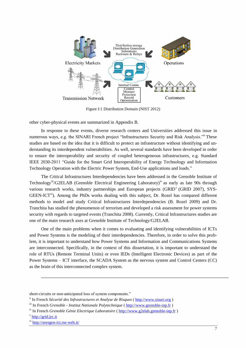
Power Systems are not an exception of the influence of ICTs, since these technologies have been progressively deployed in power systems and nowadays they are a vital part of the remote con-trol, protection and supervision systems, helping to increase the reliability, availability and safety of Power Systems. Moreover, future power networks will have a higher dependency on ICT networks, ‘Smart Grids’ will exchange communication flows with control centers, electric wholesale market, transmission network, end-users, distributed storage and distributed generation; and internal commu-nication flows between control, measure and protection components, e.g. Remote Terminal Units. Figure I:1 shows the main communication flows in Distribution Systems, including Internal and Ex-ternal Communications (NIST 2012).
However, the wide integration of ICTs within Power Systems adds complexity to an already complex field, as in the case of Power Systems. Recent events showed that failures in one infrastruc-ture affect other infrastructures. For instance, the US 2003 blackout (US-Canada Power System Outage task force 2004) taught us that the electrical grids are vulnerable and that a failure in the ICT system can have catastrophic consequences on power systems. Another example is the Stuxnet worm (Falliere, Murchu and Chien 2011). It showed that cyber events can actually target specific energy infrastructures and that the level of securityi awareness in Power Systems is questionable. These and
i Defined by the NERC as: “The ability of the power system to withstand sudden disturbances such electric
7
other cyber-physical events are summarized in Appendix B.
In response to these events, diverse research centers and Universities addressed this issue in numerous ways, e.g. the SINARI French project “Infrastructures Security and Risk Analysis.”ii These studies are based on the idea that it is difficult to protect an infrastructure without identifying and un-derstanding its interdependent vulnerabilities. As well, several standards have been developed in order to ensure the interoperability and security of coupled heterogeneous infrastructures, e.g. Standard IEEE 2030-2011 “Guide for the Smart Grid Interoperability of Energy Technology and Information Technology Operation with the Electric Power System, End-Use applications and loads.”
The Critical Infrastructures Interdependencies have been addressed in the Grenoble Institute of Technologyiii /G2ELAB (Grenoble Electrical Engineering Laboratory)iv as early as late 90s through various research works, industry partnerships and European projects (GRIDv (GRID 2007), SYS-GEEN-ICTvi). Among the PhDs works dealing with this subject, Dr. Rozel has compared different methods to model and study Critical Infrastructures Interdependencies (B. Rozel 2009) and Dr. Tranchita has studied the phenomenon of terrorism and developed a risk assessment for power systems security with regards to targeted events (Tranchita 2008). Currently, Critical Infrastructures studies are one of the main research axes at Grenoble Institute of Technology/G2ELAB.
One of the main problems when it comes to evaluating and identifying vulnerabilities of ICTs and Power Systems is the modeling of their interdependencies. Therefore, in order to solve this prob-lem, it is important to understand how Power Systems and Information and Communications Systems are interconnected. Specifically, in the context of this dissertation, it is important to understand the role of RTUs (Remote Terminal Units) or even IEDs (Intelligent Electronic Devices) as part of the Power Systems – ICT interface, the SCADA System as the nervous system and Control Centers (CC) as the brain of this interconnected complex system.
short-circuits or non-anticipated loss of system components.” ii In French Sécurité des Infrastructures et Analyse de Risques ( http://www.sinari.org ) iii In French Grenoble - Institut Nationale Polytechnique ( http://www.grenoble-inp.fr ) iv In French Grenoble Génie Electrique Laboratoire ( http://www.g2elab.grenoble-inp.fr ) v http://grid.jrc.it vi http://seesgen-ict.rse-web.it/
Figure I:1 Distribution Domain (NIST 2012)
8
This Chapter is structured in the following sections:
Section I.2 offers a general overview of CIs and their interdependencies.
Section I.3 presents a brief introduction to Power Systems and the new paradigm of Liberal-ized Power Systems.
Section I.4 addresses the control systems on electric power systems.
Section I.5 presents the interdependencies and threats between Power Systems and ICTs.
Section I.6 presents a summary and concludes with the key objectives of the dissertation.
I.2 Critical Infrastructures (CIs)
I.2.1 Definitions
The term “Critical Infrastructure” (CI) is evolving, as indicated in (O'Rourke 2007). In the 1980’s, it appeared in many policy debates. However, it was in 1996 that the term CI was used by the first time in terms of National Security (President of the US 1996). Currently, there are several defini-tions of Critical Infrastructures.
The Commission of the European Communities (European Union 2008) is defining a Critical infrastructure as: “an asset, system of part thereof located in Member States which are essential for the maintenance of vital societal functions, health, safety, security, economic or social well-being of
people, and the disruption or destruction of which would have a significant impact in a Member State as a result of the failure to maintain those functions.”
European critical infrastructures classification includes (Commission of the European Communities 2004):
Energy installations and networks;
Communications and information technologies;
Finance (banking, securities and investment);
Health care;
Food;
Water (dams, storage, treatment and networks);
Transport (airports, ports, intermodal facilities, railway and mass transit networks and traf-fic control systems);
Production, storage and transport of dangerous goods (e.g. chemical, biological, radiologi-cal and nuclear materials);
Government (e.g. critical services, facilities, information networks, assets and key national sites and monuments).
Likewise, the US Department of Homeland Security identified 18 Critical Infrastructure Sec-tors, showed in Table I:1, and defined CIs as “assets, systems, and networks, whether physical or vir-tual, so vital to the United States that their incapacitation or destruction would have a debilitating
effect on security, national economic security, public health or safety, or any combination thereof ” (US Department of Homeland Security 2009).
9
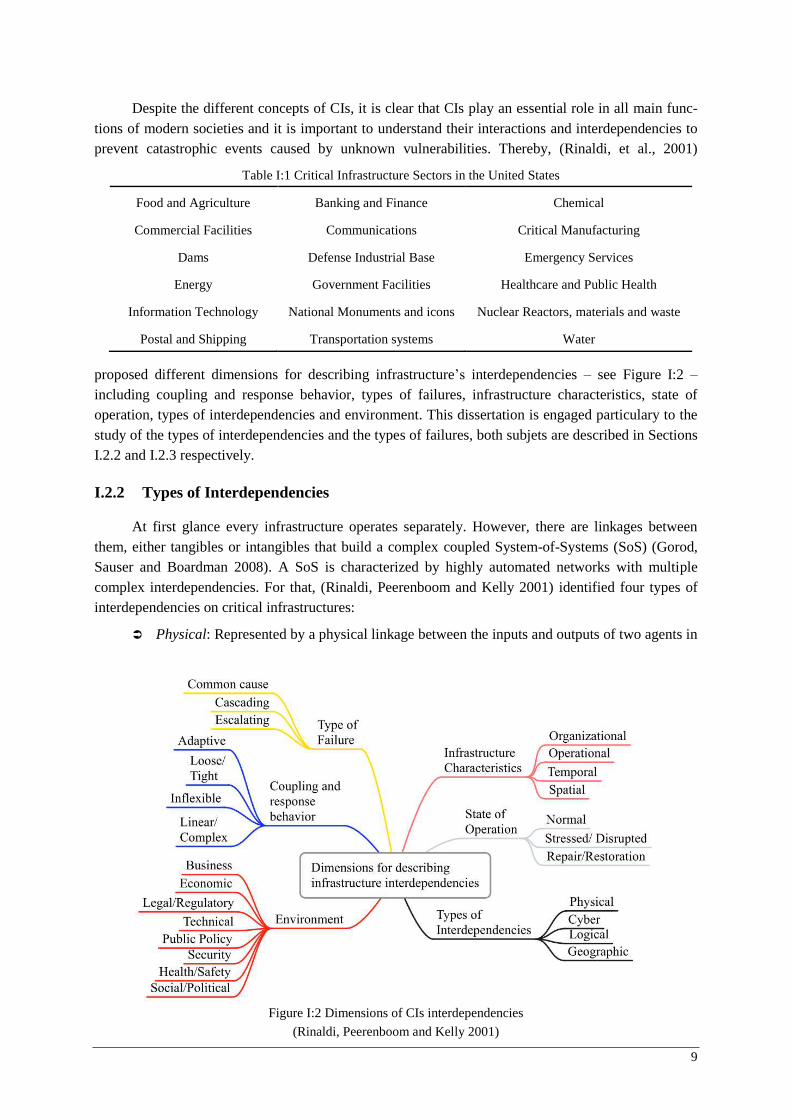
Despite the different concepts of CIs, it is clear that CIs play an essential role in all main func-tions of modern societies and it is important to understand their interactions and interdependencies to prevent catastrophic events caused by unknown vulnerabilities. Thereby, (Rinaldi, et al., 2001)
proposed different dimensions for describing infrastructure’s interdependencies – see Figure I:2 – including coupling and response behavior, types of failures, infrastructure characteristics, state of operation, types of interdependencies and environment. This dissertation is engaged particulary to the study of the types of interdependencies and the types of failures, both subjets are described in Sections I.2.2 and I.2.3 respectively.
I.2.2 Types of Interdependencies
At first glance every infrastructure operates separately. However, there are linkages between them, either tangibles or intangibles that build a complex coupled System-of-Systems (SoS) (Gorod, Sauser and Boardman 2008). A SoS is characterized by highly automated networks with multiple complex interdependencies. For that, (Rinaldi, Peerenboom and Kelly 2001) identified four types of interdependencies on critical infrastructures:
Physical: Represented by a physical linkage between the inputs and outputs of two agents in
Table I:1 Critical Infrastructure Sectors in the United States
Food and Agriculture Banking and Finance Chemical
Commercial Facilities Communications Critical Manufacturing
Dams Defense Industrial Base Emergency Services
Energy Government Facilities Healthcare and Public Health
Information Technology National Monuments and icons Nuclear Reactors, materials and waste
Postal and Shipping Transportation systems Water
Figure I:2 Dimensions of CIs interdependencies
(Rinaldi, Peerenboom and Kelly 2001)
10
different infrastructures, e.g. power systems supply power to oil infrastructures for pump stations and control systems.
Cyber: connects the state of one infrastructure to others, depending on information transmit-ted through the communications infrastructure, e.g. water facilities depend on ICT to super-vise and monitor the water pumping and cooling. (Kröger and Zio 2011) proposed to call it “Informational,” in order to include hardware and software.
Geographic: Infrastructures geographically located at the same place, where a single event can negatively affect them, e.g. in power substations when a transformer explodes and the fire burns communication cables, affecting the information and communication system. (Kröger and Zio 2011) proposed to call it “geospatial.”
Logical: When the state of one infrastructure depends on the state of another infrastructure via a connection that is not physical, cyber nor geographic, e.g. the European outage in 2006, despite it was a 30 minutes outage, French relief centers were inundated with calls (UCTE 2007). (D. Watts 2004) describes this type of interdependency in many areas be-sides critical infrastructures.
(De Porcellinis, et al. 2008) proposes a fifth interdependency called ‘Social’, when the function-ing of the whole system relies on the human behavior and activities, e.g. when a worker’s strike blocks off train rails.
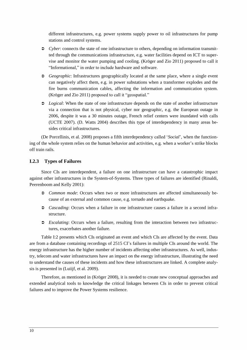
I.2.3 Types of Failures
Since CIs are interdependent, a failure on one infrastructure can have a catastrophic impact against other infrastructures in the System-of-Systems. Three types of failures are identified (Rinaldi, Peerenboom and Kelly 2001):
Common mode: Occurs when two or more infrastructures are affected simultaneously be-cause of an external and common cause, e.g. tornado and earthquake.
Cascading: Occurs when a failure in one infrastructure causes a failure in a second infra-structure.
Escalating: Occurs when a failure, resulting from the interaction between two infrastruc-tures, exacerbates another failure.
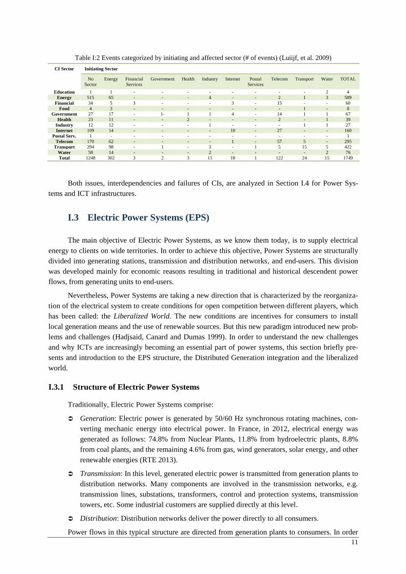
Table I:2 presents which CIs originated an event and which CIs are affected by the event. Data are from a database containing recordings of 2515 CI’s failures in multiple CIs around the world. The energy infrastructure has the higher number of incidents affecting other infrastructures. As well, indus-try, telecom and water infrastructures have an impact on the energy infrastructure, illustrating the need to understand the causes of these incidents and how these infrastructures are linked. A complete analy-sis is presented in (Luiijf, et al. 2009).
Therefore, as mentioned in (Kröger 2008), it is needed to create new conceptual approaches and extended analytical tools to knowledge the critical linkages between CIs in order to prevent critical failures and to improve the Power Systems resilience.
11
Both issues, interdependencies and failures of CIs, are analyzed in Section I.4 for Power Sys-tems and ICT infrastructures.
I.3 Electric Power Systems (EPS)
The main objective of Electric Power Systems, as we know them today, is to supply electrical energy to clients on wide territories. In order to achieve this objective, Power Systems are structurally divided into generating stations, transmission and distribution networks, and end-users. This division was developed mainly for economic reasons resulting in traditional and historical descendent power flows, from generating units to end-users.
Nevertheless, Power Systems are taking a new direction that is characterized by the reorganiza-tion of the electrical system to create conditions for open competition between different players, which has been called: the Liberalized World. The new conditions are incentives for consumers to install local generation means and the use of renewable sources. But this new paradigm introduced new prob-lems and challenges (Hadjsaid, Canard and Dumas 1999). In order to understand the new challenges and why ICTs are increasingly becoming an essential part of power systems, this section briefly pre-sents and introduction to the EPS structure, the Distributed Generation integration and the liberalized world.
I.3.1 Structure of Electric Power Systems
Traditionally, Electric Power Systems comprise:
Generation: Electric power is generated by 50/60 Hz synchronous rotating machines, con-verting mechanic energy into electrical power. In France, in 2012, electrical energy was generated as follows: 74.8% from Nuclear Plants, 11.8% from hydroelectric plants, 8.8% from coal plants, and the remaining 4.6% from gas, wind generators, solar energy, and other renewable energies (RTE 2013).
Transmission: In this level, generated electric power is transmitted from generation plants to distribution networks. Many components are involved in the transmission networks, e.g. transmission lines, substations, transformers, control and protection systems, transmission towers, etc. Some industrial customers are supplied directly at this level.
Distribution: Distribution networks deliver the power directly to all consumers.
Power flows in this typical structure are directed from generation plants to consumers. In order
Table I:2 Events categorized by initiating and affected sector (# of events) (Luiijf, et al. 2009)
CI Sector Initiating Sector
No Sector
Energy Financial Services
Government Health Industry Internet Postal Services
Telecom Transport Water TOTAL
Education 1 1 - - - - - - - - 2 4 Energy 515 65 - - - 4 - - 2 1 3 589
Financial 34 5 3 - - - 3 - 15 - - 60 Food 4 3 - - - - - - - 1 - 8
Government 27 17 - 1- 1 1 4 - 14 1 1 67 Health 23 11 - - 2 - - - 2 - 1 39
Industry 12 12 - - - 1 - - - 1 1 27 Internet 109 14 - - - - 10 - 27 - - 160
Postal Serv. 1 - - - - - - - - - - 1 Telecom 170 62 - - - - 1 - 57 5 - 295
Transport 294 98 - 1 - 3 - 1 5 15 5 422 Water 58 14 - - - 2 - - - - 2 76 Total 1248 302 3 2 3 11 18 1 122 24 15 1749
12
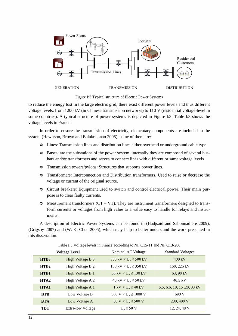
to reduce the energy lost in the large electric grid, there exist different power levels and thus different voltage levels, from 1200 kV (in Chinese transmission networks) to 110 V (residential voltage-level in some countries). A typical structure of power systems is depicted in Figure I:3. Table I:3 shows the voltage levels in France.
In order to ensure the transmission of electricity, elementary components are included in the system (Hewitson, Brown and Balakrishnan 2005), some of them are:
Lines: Transmission lines and distribution lines either overhead or underground cable type.
Buses: are the substations of the power system, internally they are composed of several bus-bars and/or transformers and serves to connect lines with different or same voltage levels.
Transmission towers/pylons: Structures that supports power lines.
Transformers: Interconnection and Distribution transformers. Used to raise or decrease the voltage or current of the original source.
Circuit breakers: Equipment used to switch and control electrical power. Their main pur-pose is to clear faulty currents.
Measurement transformers (CT – VT): They are instrument transformers designed to trans-form currents or voltages from high value to a value easy to handle for relays and instru-ments.
A description of Electric Power Systems can be found in (Hadjsaid and Sabonnadière 2009), (Grigsby 2007) and (W.-K. Chen 2005), which may help to better understand the work presented in this dissertation.
Table I:3 Voltage levels in France according to NF C15-11 and NF C13-200
Voltage Level Nominal AC Voltage Standard Voltages
HTB3 High Voltage B 3 350 kV < Un ≤ 500 kV 400 kV
HTB2 High Voltage B 2 130 kV < Un ≤ 350 kV 150, 225 kV
HTB1 High Voltage B 1 50 kV < Un ≤ 130 kV 63, 90 kV
HTA2 High Voltage A 2 40 kV < Un ≤ 50 kV 40.5 kV
HTA1 High Voltage A 1 1 kV < Un ≤ 40 kV 5.5, 6.6, 10, 15 ,20, 33 kV
BTB Low Voltage B 500 V < Un ≤ 1000 V 690 V
BTA Low Voltage A 50 V < Un ≤ 500 V 230, 400 V
TBT Extra-low Voltage Un ≤ 50 V 12, 24, 48 V
Figure I:3 Typical structure of Electric Power Systems
13
I.3.2 The Liberalized World and the Distributed Generation (DG)
Back in 1978, the Public Utility Regulatory Policies Act (PURPA) was presented in the United States; this act determined the beginning of the deregulation process (first free-market approach) and promoted the research on novel and sustainable technologies, to produce electricity from renewable sources such as water, wind or solar power.
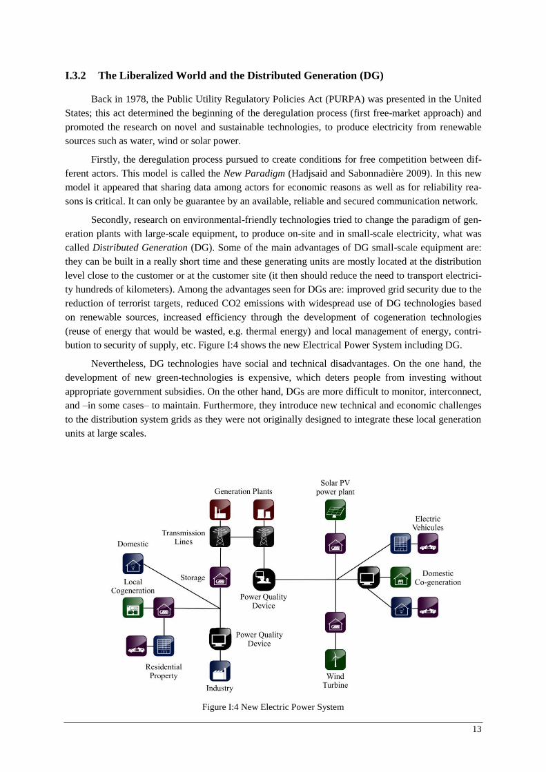
Firstly, the deregulation process pursued to create conditions for free competition between dif-ferent actors. This model is called the New Paradigm (Hadjsaid and Sabonnadière 2009). In this new model it appeared that sharing data among actors for economic reasons as well as for reliability rea-sons is critical. It can only be guarantee by an available, reliable and secured communication network.
Secondly, research on environmental-friendly technologies tried to change the paradigm of gen-eration plants with large-scale equipment, to produce on-site and in small-scale electricity, what was called Distributed Generation (DG). Some of the main advantages of DG small-scale equipment are: they can be built in a really short time and these generating units are mostly located at the distribution level close to the customer or at the customer site (it then should reduce the need to transport electrici-ty hundreds of kilometers). Among the advantages seen for DGs are: improved grid security due to the reduction of terrorist targets, reduced CO2 emissions with widespread use of DG technologies based on renewable sources, increased efficiency through the development of cogeneration technologies (reuse of energy that would be wasted, e.g. thermal energy) and local management of energy, contri-bution to security of supply, etc. Figure I:4 shows the new Electrical Power System including DG.
Nevertheless, DG technologies have social and technical disadvantages. On the one hand, the development of new green-technologies is expensive, which deters people from investing without appropriate government subsidies. On the other hand, DGs are more difficult to monitor, interconnect, and –in some cases– to maintain. Furthermore, they introduce new technical and economic challenges to the distribution system grids as they were not originally designed to integrate these local generation units at large scales.
Figure I:4 New Electric Power System
14
I.4 ICTs for Power Systems
Markets liberalization and distributed generation deployment led to profound modifications in the structure of the electric power system. That is, from ‘quasi-monopoly’ system to an open access offering market conditions to companies.
Market competition requires transparency and symmetry of information. Therefore, it is manda-tory to share real-time information and to ensure a controlled, protected and monitored system. For this reason, many Information and Communication Technologies were distributed in the electric pow-er grids; these technologies are able to acquire, store, process system measures and commands (PSERC 2012).
Some of the main applications of ICTs on power grids, control strategies for distribution power systems, control assets and critical threats to ICT and power systems are presented in this section.
I.4.1 Control assets of EPS
Supply of high quality electricity, in constrained power system, is difficult to achieve without a continuous knowledge of the state of the electric power system. For this reason, on-field instrumenta-tion and communication technologies are used to acquire and send measurements via a telecommuni-cations infrastructure to a control center. Control centers process the data and find the appropriate commands to maintain the electrical parameters within an acceptable range. Some of these assets comprise: Remote Terminal Units, Programmable Logic Controller (PLC), Intelligent Electronic De-vices (IEDs), Human Machine Interface (HMI), and Supervisory Control And Data Acquisition SCADA System (Knapp 2011), (Galloway and Hancke 2012), (Gönen 2008).
I.4.1.1 Remote Terminal Units (RTUs)
RTUs are data collectors that provide connectivity (on the slave side) to the SCADA network (on the master side), since RTUs acquire field digital and analog parameters and transmit them back to a Distributed Control Systemvii (DCS) or SCADA system in a control center. RTUs are considered as the interface of the network buses in the physical layer with the cyber layers (Bompard, Cuccia, et al. 2012).
RTUs include remote communications capabilities such as wire modem, cellular data connec-tion, radio, and/or other wide area communication capabilities. As well, RTUs use industrial network protocols, mostly defined by the Standard IEEE 60870-5-104. They are microprocessor powered and use a set of analog and digital input/output channels. These channels can be implemented through various physical media such as parallel-resonant circuit on power lines carriers, telephone wires, optic fibers, radio wave and satellite communications.
Since RTUs are typically located in substations or in a remote location, they are extremely du-rable and reliable in order to withstand harsh field conditions. The RTUs power supply is provided by a DC/DC converter and includes a battery and charger circuitry to continue operation in an event of long power outage.
vii Distributed Control Systems used to monitor and control distributed equipment.
15
I.4.1.2 Programmable Logic Controllers (PLCs)
PLCs automate functions on EPS. They are specialized computers with multiple analogical or numerical inputs/outputs. PLCs rely on blocks of logic code allowing them to automatically operate to specific signals, e.g. from a relay or a sensor. They are programmed using specialized software (e.g. Simatic Step 7, Unity Pro) on personal computers. PLCs include built-in communication ports such as series RS-232 or Ethernet, using Modbus, DF1 protocols among others, thus they can be connected to a computer running SCADA. They are more intelligent than RTUs and have the ability to issue con-trols without taking direction from a Master Unit.
I.4.1.3 Intelligent Electronic Devices (IEDs)
An IED is any device from the RTU family with signal processing as well as control and com-munication abilities that is equipped with a small microprocessor and is able to receive or send da-ta/control from/to an external source. IEDs use fieldbus protocols and include functions and features such as self-check, diagnostics and historical data store.
I.4.1.4 Supervisory Control and Data Acquisition (SCADA)
One of the multiple definitions of SCADA is: “SCADA is the equipment and procedures for
controlling one or more remote stations from a master control station. It includes the digital control equipment, sensing and telemetry equipment, and two-way communications to and from the master
stations and the remotely controlled stations” (Gönen 2008, 216)
However, there are disagreements among experts. For instance, it can be found definitions like: “A SCADA system is a purely software layer, normally applied a level above control hardware within
the hierarchy of an industrial network.” In fact, there is still a discussion between control engineers about the definition of Industrial Control System (ICS) and SCADA System (Byres 2012).
The definition of the SCADA retained in this thesis is an information system that allows the transfer of remote commands, annunciation and telemetry signals necessary to the monitoring and control of the electric power system.
Master Terminal Units are known as the heart of the SCADA system. MTUs are located at the operator’s control center facility. The data from all RTUs in remote sites are sent to the MTU to be processed and stored.
HMIs are the interface between the Operator (Human) and the electric power system (machine). They play a vital role for systems’ automation since they allow important tasks such as control, moni-toring, diagnosis and managing of EPS to be processed. Through HMIs, operators open and close cir-cuit breakers, visualize current operational parameters on screens (voltages, current, and state of switchgears), adjust system values and other functions, etc. Usually, HMIs are connected to one or more PLC and RTUs. HMIs show information on text displays, graphical panels, touchscreens or web-based interfaces.
I.4.2 Automation of Electric Power Systems
In the context of automation, Electrical Power Systems are generally divided into five hierar-chical levels as shown in Figure I:5. Three levels are for Substation Automation Systems: Process level, bay level and station level. The other two levels are: the regional control center (RCC) level and the national control center level (NCC).
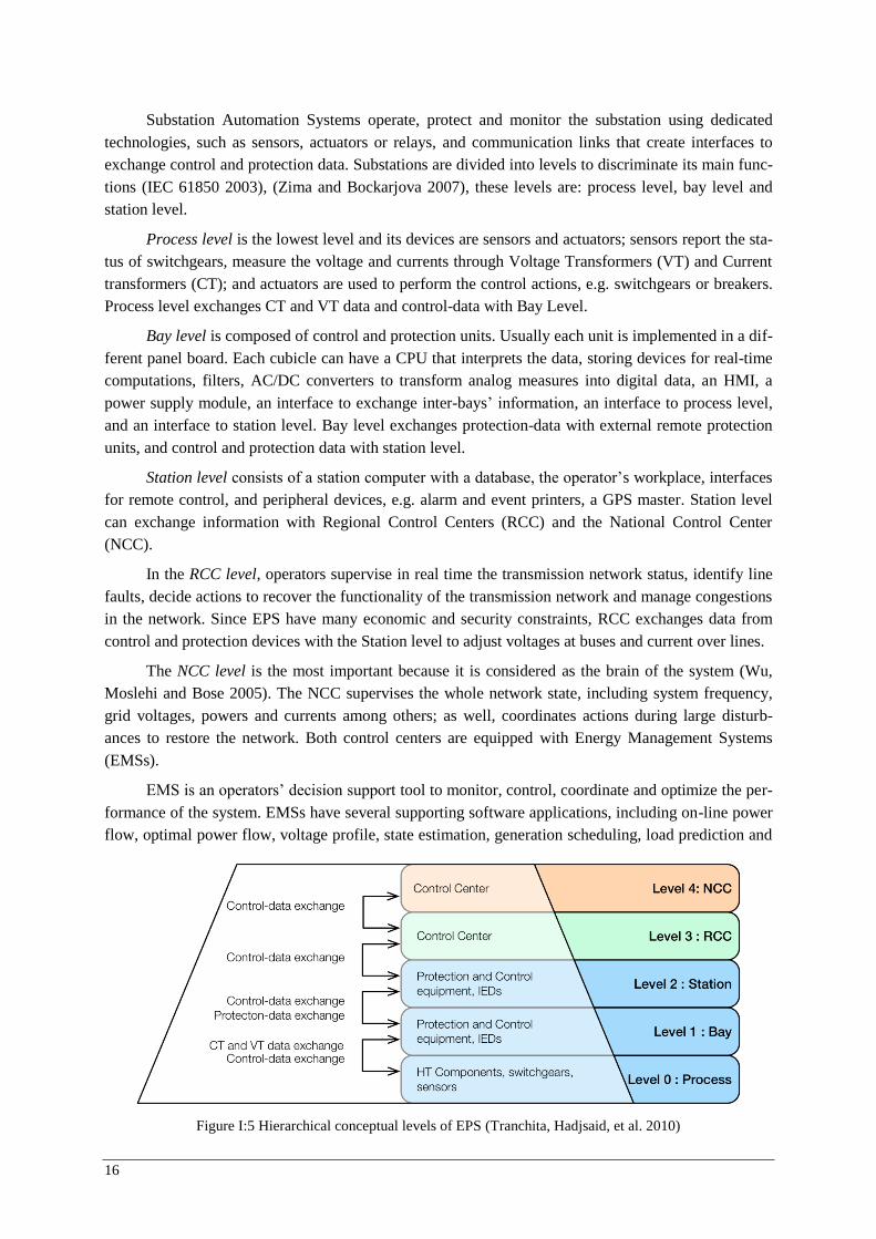
16
Substation Automation Systems operate, protect and monitor the substation using dedicated technologies, such as sensors, actuators or relays, and communication links that create interfaces to exchange control and protection data. Substations are divided into levels to discriminate its main func-tions (IEC 61850 2003), (Zima and Bockarjova 2007), these levels are: process level, bay level and station level.
Process level is the lowest level and its devices are sensors and actuators; sensors report the sta-tus of switchgears, measure the voltage and currents through Voltage Transformers (VT) and Current transformers (CT); and actuators are used to perform the control actions, e.g. switchgears or breakers. Process level exchanges CT and VT data and control-data with Bay Level.
Bay level is composed of control and protection units. Usually each unit is implemented in a dif-ferent panel board. Each cubicle can have a CPU that interprets the data, storing devices for real-time computations, filters, AC/DC converters to transform analog measures into digital data, an HMI, a power supply module, an interface to exchange inter-bays’ information, an interface to process level, and an interface to station level. Bay level exchanges protection-data with external remote protection units, and control and protection data with station level.
Station level consists of a station computer with a database, the operator’s workplace, interfaces for remote control, and peripheral devices, e.g. alarm and event printers, a GPS master. Station level can exchange information with Regional Control Centers (RCC) and the National Control Center (NCC).
In the RCC level, operators supervise in real time the transmission network status, identify line faults, decide actions to recover the functionality of the transmission network and manage congestions in the network. Since EPS have many economic and security constraints, RCC exchanges data from control and protection devices with the Station level to adjust voltages at buses and current over lines.
The NCC level is the most important because it is considered as the brain of the system (Wu, Moslehi and Bose 2005). The NCC supervises the whole network state, including system frequency, grid voltages, powers and currents among others; as well, coordinates actions during large disturb-ances to restore the network. Both control centers are equipped with Energy Management Systems (EMSs).
EMS is an operators’ decision support tool to monitor, control, coordinate and optimize the per-formance of the system. EMSs have several supporting software applications, including on-line power flow, optimal power flow, voltage profile, state estimation, generation scheduling, load prediction and
Figure I:5 Hierarchical conceptual levels of EPS (Tranchita, Hadjsaid, et al. 2010)
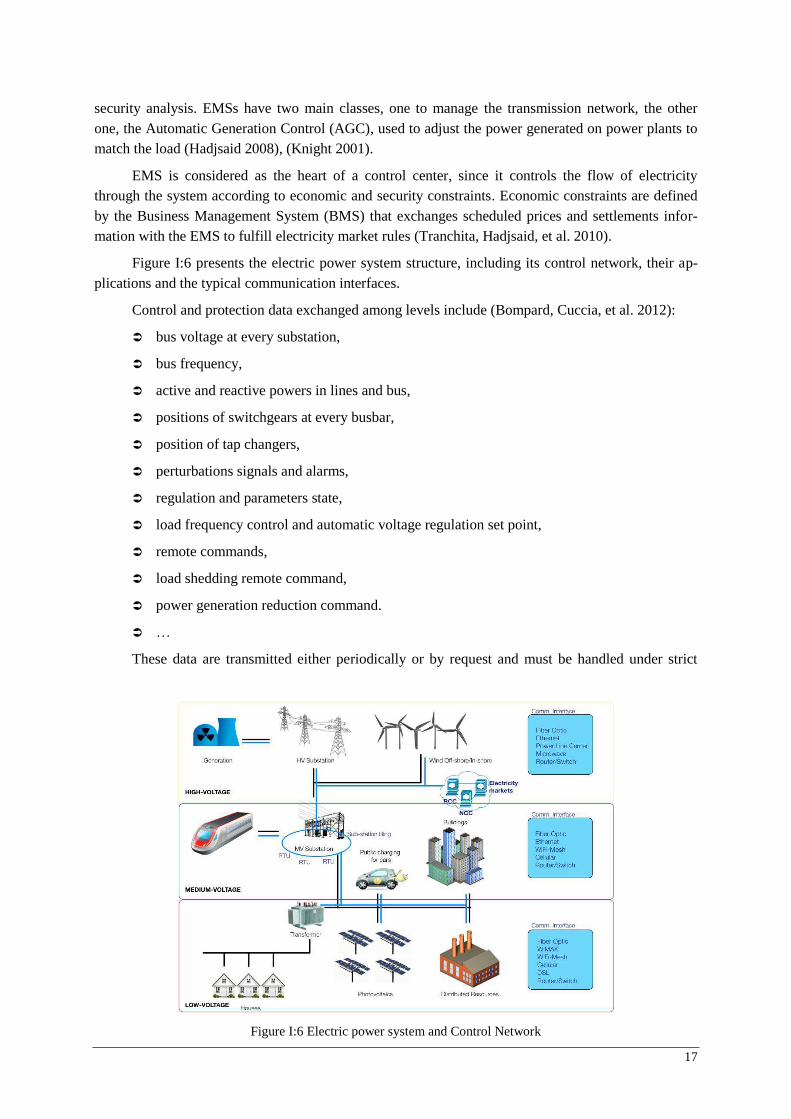
17
security analysis. EMSs have two main classes, one to manage the transmission network, the other one, the Automatic Generation Control (AGC), used to adjust the power generated on power plants to match the load (Hadjsaid 2008), (Knight 2001).
EMS is considered as the heart of a control center, since it controls the flow of electricity through the system according to economic and security constraints. Economic constraints are defined by the Business Management System (BMS) that exchanges scheduled prices and settlements infor-mation with the EMS to fulfill electricity market rules (Tranchita, Hadjsaid, et al. 2010).
Figure I:6 presents the electric power system structure, including its control network, their ap-plications and the typical communication interfaces.
Control and protection data exchanged among levels include (Bompard, Cuccia, et al. 2012):
bus voltage at every substation,
bus frequency,
active and reactive powers in lines and bus,
positions of switchgears at every busbar,
position of tap changers,
perturbations signals and alarms,
regulation and parameters state,
load frequency control and automatic voltage regulation set point,
remote commands,
load shedding remote command,
power generation reduction command.
…
These data are transmitted either periodically or by request and must be handled under strict
Figure I:6 Electric power system and Control Network
18
rules of confidentiality, acquisition, coordination and usage. Security issues handling this data and main vulnerabilities on power systems and ICT are discussed in the next section.
I.5 ICT and EPS Interdependencies
I.5.1 ICT Threats on Power Systems
As shown above, Electric Power Systems operators rely on Information and Communication Technologies to monitor and control the network. Nevertheless, there is still a critical question: Is the ICT infrastructure improving or endangering the security, the reliability and the resilience of Power Systems? Recent events (see Appendix B) revealed several facts. i) Failures in ICT infrastructure can actually affect Power Systems. ii ) There is a tendency to perform targeted cyber and physical attacks. iii ) Isolation from the internet is not an effective defense, and all power systems that are controlled by software are vulnerable to cyber threats. iv) Terrorists and war fighters recognized that it is more ef-fective to attack ICT infrastructures directly, than to physically attack their targets (Chen and Saeed 2011), (Trevorrow, et al. 2006).
Therefore, in order to study the interdependencies and vulnerabilities of Power Systems, it is important to identify the main threats for ICT and how they can affect the Power System.
In the ICT domain, information security is the process of defending information from unauthor-ized access, use, and modification. Its main objectives, according to the ANSSIviii are (ANSSI 2010):
Ensure the availability of data and information systems, i.e. information is available when it is needed;
Guarantee the integrity of information systems, i.e. originally sent information must stay unaltered;
Make sure that the data remains confidential, i.e. only authorized persons have access to the information;
Create practices to differentiate between legitimate and illegitimate users, i.e. Authenticity;
Control the changes effectuated on information and trace the person that did the changes, i.e. Traceability.
These objectives can be applied as well for Power Systems. Four cases show the criticality of these properties:
Availability: The regional control center requests load information to feed the state estima-tor, but this information is unavailable due to a Trojan that attacked the EMS (Santamarta 2011).
Integrity: An intruder changes the values of currents on power lines (virtually). Operators read on HMIs that the main transmission lines are overloaded, thus they decide to start the load shedding procedure, affecting the normal network condition (Liu, et al. 2012).
Confidentiality: A terrorist group steals sensitive documents from energy companies to plan a massive attack (Karpersky Laboratory 2012).
viii French Network and Information Security Agency (Agence nationale de sécurité des systèmes d’information).
19
Authenticity: An intruder, using social engineeringix, obtains operators’ IDs and passwords needed for substation HMI remote desktop connection (Liu, et al. 2012).
These are just some examples; however, many threats can affect the control system and conse-quently the electrical power system. There are two types of threats: internal and externals.
For instance, an internal threat can be an employee that for some reasons decides to attack the SCADA System, e.g. an employee from the Australian sewage system release million liters of water into parks of Australia (Smith 2001). Similarly, a contractor that has a temporary access to the system can attack it. These internal threats can be either an intentional attack or an accident (human error).
External threats may lack of specific origin or source. For instance, when a random malware ar-rives to the operator computers, e.g. the Nimda worm affected an EMS/SCADA system in 2001 (CERT 2001). Or it could have a specific source, natural disasters and electric phenomena on power lines can damage the control system functioning, e.g. electromagnetic interferences, noise on power lines. Finally, the most dangerous are the targeted attacks developed by terrorist, by other nations or by hacktivists, these attackers have special knowledge and a clear objective, Stuxnet worm is a well-known example (Falliere, Murchu and Chien 2011). The most common threats for ICT are: autono-mous worms, terrorists, viruses, Trojan horses, human errors, accidents, noise on power lines, and improper application of software patches (Krutz 2006).
ICT on Power Systems are vulnerable because, at the beginning, off-the-shelves technologies that were used in control centers and ICT for power systems lacked of information security as it was an insignificant requirement 30 years ago (Masera, Fovino and Vamanu 2011).
External and internal threats can exploit different unsecured attack points, among them: Blue-tooth and Wi-Fi connection, connections between SCADA systems and other Local Area Networks (LANs), corporate Web servers, email servers, internet gateways, open computer ports, poor config-ured firewalls, and weak authentication protocols (Sridhar and Govindarasu 2012). Authors in (Bompard, Cuccia, et al. 2012) classify these vulnerabilities into four categories:
i) SCADA system weaknesses: they are mainly protocol weaknesses, e.g. unauthorized com-mand execution, SCADA denial-of-service, man-in-the-middle, and worm attacks. These at-tacks can have negative consequences on the industrial operation and by cascading on other infrastructures.
ii) Process network weaknesses: they allow the control of the SCADA server to be taken, inter-rupting communication flows or sending unauthorized commands.
iii) Control center weaknesses: they include virus infections and attacks with false authentica-tion on computers, mainly for HMI purposes.
iv) Network layer weaknesses: they cover routing attack or intentional disconnection of the communication network.
ICTs threats are growing for all infrastructures particularly for the energy sector. According to McAfee, 60 million malware programs are written every year. In only one year cyberattacks against federal networks have increased about 40% (Motorola 2012). According to the ICS-CERT, 41.4% of the cyber-attacks against critical infrastructures where against the Energy Sector, Figure I:7 shows the results of the study (ICS-CERT 2012).
ix Social engineering is the use of cultural ploys and psychological manipulation to get confidential information to illegally intrude on computer systems or networks (Abraham and Chergalur-Smith 2010).
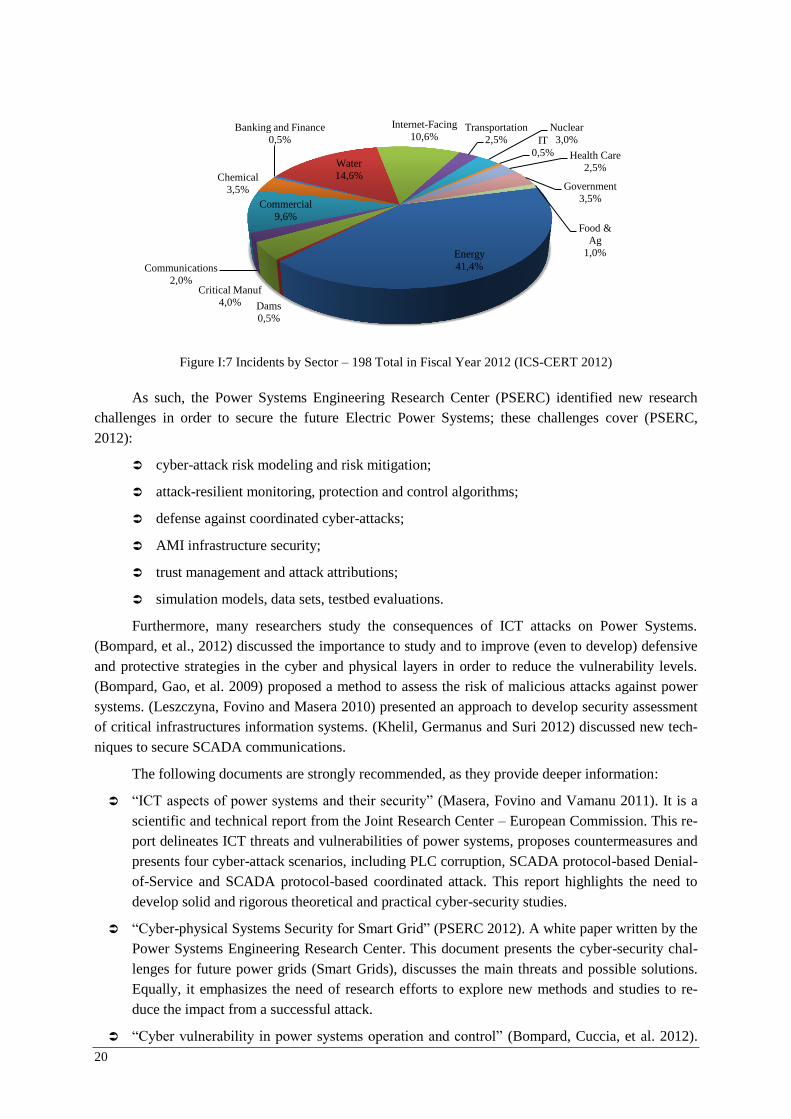
20
As such, the Power Systems Engineering Research Center (PSERC) identified new research challenges in order to secure the future Electric Power Systems; these challenges cover (PSERC, 2012):
cyber-attack risk modeling and risk mitigation;
attack-resilient monitoring, protection and control algorithms;
defense against coordinated cyber-attacks;
AMI infrastructure security;
trust management and attack attributions;
simulation models, data sets, testbed evaluations.
Furthermore, many researchers study the consequences of ICT attacks on Power Systems. (Bompard, et al., 2012) discussed the importance to study and to improve (even to develop) defensive and protective strategies in the cyber and physical layers in order to reduce the vulnerability levels. (Bompard, Gao, et al. 2009) proposed a method to assess the risk of malicious attacks against power systems. (Leszczyna, Fovino and Masera 2010) presented an approach to develop security assessment of critical infrastructures information systems. (Khelil, Germanus and Suri 2012) discussed new tech-niques to secure SCADA communications.
The following documents are strongly recommended, as they provide deeper information:
“ICT aspects of power systems and their security” (Masera, Fovino and Vamanu 2011). It is a scientific and technical report from the Joint Research Center – European Commission. This re-port delineates ICT threats and vulnerabilities of power systems, proposes countermeasures and presents four cyber-attack scenarios, including PLC corruption, SCADA protocol-based Denial-of-Service and SCADA protocol-based coordinated attack. This report highlights the need to develop solid and rigorous theoretical and practical cyber-security studies.
“Cyber-physical Systems Security for Smart Grid” (PSERC 2012). A white paper written by the Power Systems Engineering Research Center. This document presents the cyber-security chal-lenges for future power grids (Smart Grids), discusses the main threats and possible solutions. Equally, it emphasizes the need of research efforts to explore new methods and studies to re-duce the impact from a successful attack.
“Cyber vulnerability in power systems operation and control” (Bompard, Cuccia, et al. 2012).
Figure I:7 Incidents by Sector – 198 Total in Fiscal Year 2012 (ICS-CERT 2012)
Energy 41,4%
Dams 0,5%
Critical Manuf 4,0%
Communications 2,0%
Commercial 9,6%
Chemical 3,5%
Banking and Finance 0,5%
Water 14,6%
Internet-Facing 10,6%
Transportation 2,5%
Nuclear 3,0% IT
0,5% Health Care 2,5%
Government 3,5%
Food & Ag
1,0%
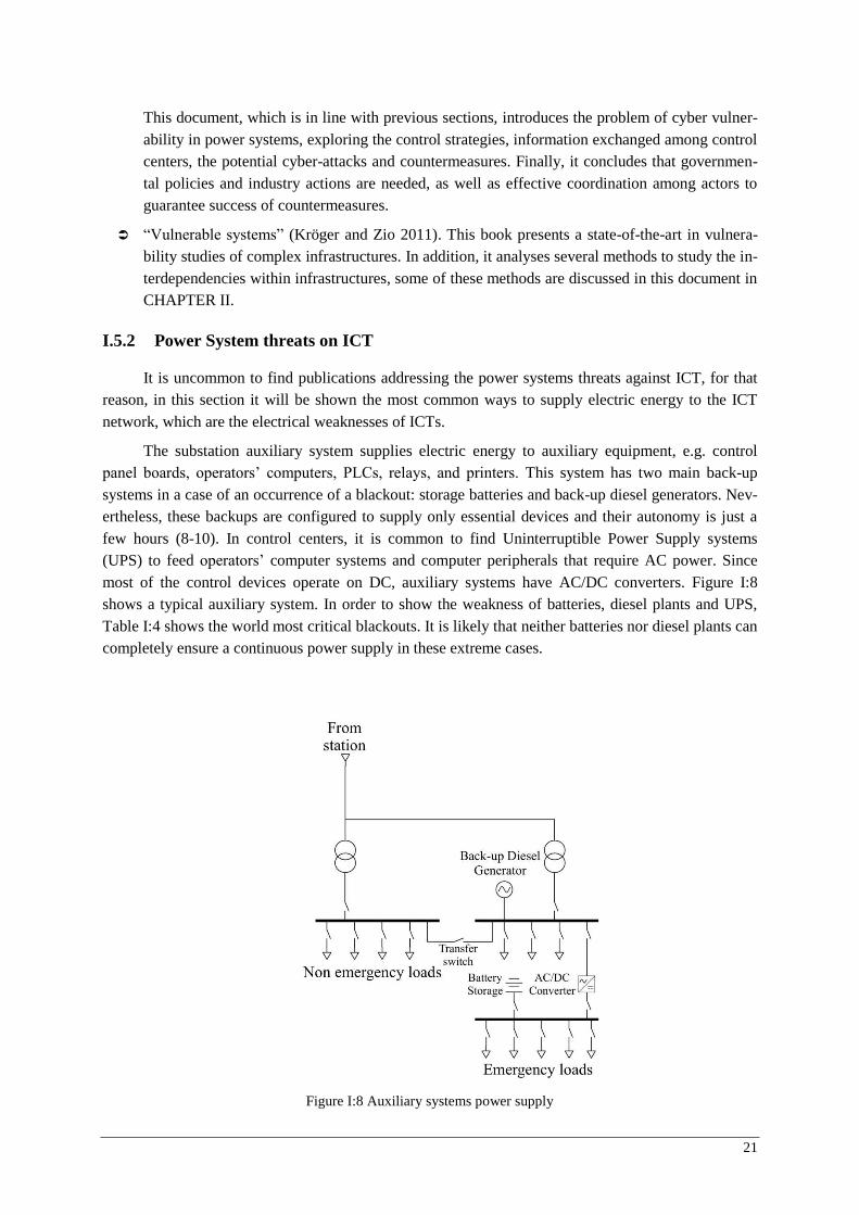
21
This document, which is in line with previous sections, introduces the problem of cyber vulner-ability in power systems, exploring the control strategies, information exchanged among control centers, the potential cyber-attacks and countermeasures. Finally, it concludes that governmen-tal policies and industry actions are needed, as well as effective coordination among actors to guarantee success of countermeasures.
“Vulnerable systems” (Kröger and Zio 2011). This book presents a state-of-the-art in vulnera-bility studies of complex infrastructures. In addition, it analyses several methods to study the in-terdependencies within infrastructures, some of these methods are discussed in this document in CHAPTER II.
I.5.2 Power System threats on ICT
It is uncommon to find publications addressing the power systems threats against ICT, for that reason, in this section it will be shown the most common ways to supply electric energy to the ICT network, which are the electrical weaknesses of ICTs.
The substation auxiliary system supplies electric energy to auxiliary equipment, e.g. control panel boards, operators’ computers, PLCs, relays, and printers. This system has two main back-up systems in a case of an occurrence of a blackout: storage batteries and back-up diesel generators. Nev-ertheless, these backups are configured to supply only essential devices and their autonomy is just a few hours (8-10). In control centers, it is common to find Uninterruptible Power Supply systems (UPS) to feed operators’ computer systems and computer peripherals that require AC power. Since most of the control devices operate on DC, auxiliary systems have AC/DC converters. Figure I:8 shows a typical auxiliary system. In order to show the weakness of batteries, diesel plants and UPS, Table I:4 shows the world most critical blackouts. It is likely that neither batteries nor diesel plants can completely ensure a continuous power supply in these extreme cases.
Figure I:8 Auxiliary systems power supply

22
I.6 Summary
Power systems have faced several changes over their history while improving their reliability and availability. The end of the XXth century was marked by a massive deployment of information and communication technologies, including computers, satellites, fiber optics, among others. Recently, power systems have experienced two significant changes: energy market liberalization and insertion of decentralized/distributed generation. Both changes require a secure, optimal, fast and bi-directional communication among players, these players can be at the same time consumers and producers: ‘Prosumers.’
Information and Communication Technologies (ICTs) have been a very positive improvement for power systems because they support not only the supervision and control of power systems, but also the operation decisions, policy making and markets regulation.
However, deployment of ICTs in power systems added a new complexity to study the reliability and resilience of power systems. This new complexity is divided into multiple layers, charactering the different types of interdependencies within coupled infrastructures. Therefore, it is important to define a micro and macro vision of the interdependencies between these infrastructures, having the power system at the center of other infrastructures as their power supply.
Similarly, ICT’s are vulnerable to several threats. Virus, malwares, Denial-of-service attacks are some of the attacks that can affect the normal operation of ICT’s and, consequently, power systems. Furthermore, power systems blackouts can affect ICT.
Since Power Systems and Information and Communication Technologies are considered as vital for the society, they are included as Critical Infrastructures by the US-Government and the European Commission. Consequently, it is of high importance to study their interactions and how to protect them from attacks.
Table I:4 Longest blackouts
Country Date Worst Duration Case Population in-volved
New Zealand 20.02.1998 >1 week 70 000
Brazil 11.03.1999 5 hours 97 000 000
United States 14.08.2003 > 1 day 55 000 000
Italy 28.09.2003 18 hours 56 000 000
Indonesia 18.08.2005 > 5 hours 100 000 000
Brazil 04.02.2011 >7 hours 53 000 000
India 30.07.2012 > 6 hours 670 000 000

23
The specific objectives of this dissertation are:
To compare the different approaches to model coupled infrastructures and to identify the main advantages and disadvantages.
To analyze the different properties of Complex Networks in order to identify those that will allow us to model the coupled infrastructures.
To propose different approaches that enable the study of coupled infrastructures, including the different interdependencies layers.
To compare and analyze the main advantages and disadvantages of the proposed approach-es.
To explore the feasibility of using the proposed approaches at different levels, according to the most recent architectures proposed for Smart Grids.

25
CHAPTER II Modeling Critical Infrastructures: State-of-the-art
The need to be right is the sign of a vulgar mind.
Albert Camus
TABLE OF CONTENTS
II.1 INTRODUCTION .............................................................................................................. 26
II.2 COMPLEX NETWORKS ................................................................................................... 27
II.2.1 Initiating event and cascade-safe operating margins ......................................... 27
II.2.2 Global vulnerability of interdependent infrastructures ..................................... 27
II.2.3 Interdependent technical infrastructures modeling ........................................... 28
II.2.4 Rule-based complex networks .......................................................................... 29
II.2.5 Advantages – Disadvantages............................................................................. 29
II.3 AGENT-BASED MODEL (ABM) ..................................................................................... 30
II.3.1 Object-Oriented Hybrid Modeling Approach ................................................... 31
II.3.2 Agent-based input-output interdependency model ........................................... 32
II.3.3 Federated Agent-Based model .......................................................................... 32
II.3.4 Advantages - Disadvantages ............................................................................. 33
II.4 BAYESIAN NETWORKS (BN) ......................................................................................... 34
II.4.1 Cause-Effect interdependencies ........................................................................ 34
II.4.2 Dynamic Bayesian Networks ............................................................................ 35
II.4.3 Advantages - Disadvantages ............................................................................. 36
II.5 BOOLEAN LOGIC DRIVEN MARKOV PROCESSES ........................................................... 36
II.6 COMBINED SIMULATORS ............................................................................................... 37
II.6.1 Cosimulator for Transport and Distribution systems ........................................ 37
II.6.2 Real-time Cosimulator ...................................................................................... 38
II.6.3 Federate-based Simulator .................................................................................. 39
II.6.4 Agent-based simulation tool: EPOCHS ............................................................ 40
II.6.5 Advantages - Disadvantages ............................................................................. 41
II.7 PETRI NETWORKS (PN) ................................................................................................. 41
26
II.7.1 Attack/Defense modeling .................................................................................. 42
II.7.2 “High-level” and “Low-level” Petri Nets ......................................................... 43
II.7.3 SWN and SAN integration ................................................................................ 43
II.7.4 Intrusion detection on Cyber Physical Systems ................................................ 44
II.7.5 Advantages - Disadvantages ............................................................................. 44
II.8 COMPARISON AND CONCLUSION ................................................................................... 44
Abstract
Critical infrastructures’ modeling needs a multidisciplinary approach in order to study and understand
their interdependencies and vulnerabilities in a complex interconnected world. This Chapter presents a state-of-
the-art on modeling methods for identifying and understanding the interdependencies among Critical Infrastruc-
tures, including: Complex Networks, Agent-based models, Bayesian Networks, Boolean Logic Driven Markov
processes and Petri networks. Different approaches are described and a summary of main advantages, disad-
vantages and limitations are then discussed. Finally, this Chapter presents a comparison of these methods, con-
sidering the usability, the ability to handle large complex systems, the scalability, among others.
II.1 Introduction
CHAPTER I reveals that power systems and ICT infrastructures are highly interdependent and failures in one infrastructure can affect the other infrastructure. In order to tackle this difficult prob-lem, it is important to develop modeling methods to identify possible common defaults, consequences of cascading failures and vulnerabilities of coupled infrastructures.
Therefore, research efforts were addressed to study the interdependencies of coupled infrastruc-tures. In the past, computer processing capacity restricted the development of theories and methods to analyze complex interdependent critical infrastructures. However, after the boost of computational power, computer evolution has significantly supported the development of new theories and method-ologies. Thus, the set of theories that were formulated at the beginning of the XXth century have rap-idly progressed.
Nevertheless, classical methods, such as Failure Mode and Effects Analysis (FMEA), fault trees, Monte Carlo or lifetime assessment (Benbow and Broome 2009), did not provide the infor-mation and the tools required to understand complex coupled infrastructure. Therefore, many non-classical methods have arisen to explain and to help the understanding of coupled infrastructures, in-cluding: Agents-based modeling and simulation, Bayesian Networks, Boolean Logic Driven Markov Processes, Complex Networks, Combined Simulation, Petri Networks, Supply/Demand graphs and others.
This Chapter presents some approaches based on the non-classical methods, followed by a dis-cussion about the main advantages, disadvantages and limitations of each method. At the end of the Chapter, these methods are compared taking into account the CPU consumption, the usability, the ability to model large and complex systems, the scalability, the ability to perform dynamic simulations and the availability of robust tools to compute them.
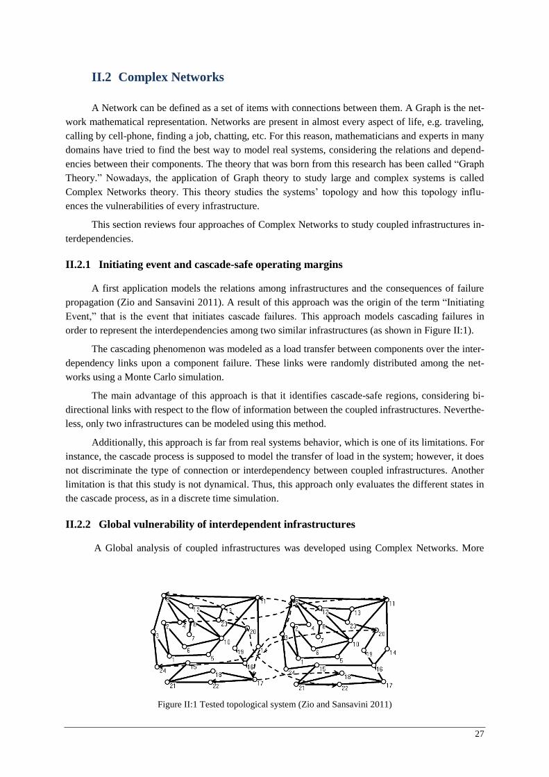
27
II.2 Complex Networks
A Network can be defined as a set of items with connections between them. A Graph is the net-work mathematical representation. Networks are present in almost every aspect of life, e.g. traveling, calling by cell-phone, finding a job, chatting, etc. For this reason, mathematicians and experts in many domains have tried to find the best way to model real systems, considering the relations and depend-encies between their components. The theory that was born from this research has been called “Graph Theory.” Nowadays, the application of Graph theory to study large and complex systems is called Complex Networks theory. This theory studies the systems’ topology and how this topology influ-ences the vulnerabilities of every infrastructure.
This section reviews four approaches of Complex Networks to study coupled infrastructures in-terdependencies.
II.2.1 Initiating event and cascade-safe operating margins
A first application models the relations among infrastructures and the consequences of failure propagation (Zio and Sansavini 2011). A result of this approach was the origin of the term “Initiating Event,” that is the event that initiates cascade failures. This approach models cascading failures in order to represent the interdependencies among two similar infrastructures (as shown in Figure II :1).
The cascading phenomenon was modeled as a load transfer between components over the inter-dependency links upon a component failure. These links were randomly distributed among the net-works using a Monte Carlo simulation.
The main advantage of this approach is that it identifies cascade-safe regions, considering bi-directional links with respect to the flow of information between the coupled infrastructures. Neverthe-less, only two infrastructures can be modeled using this method.
Additionally, this approach is far from real systems behavior, which is one of its limitations. For instance, the cascade process is supposed to model the transfer of load in the system; however, it does not discriminate the type of connection or interdependency between coupled infrastructures. Another limitation is that this study is not dynamical. Thus, this approach only evaluates the different states in the cascade process, as in a discrete time simulation.
II.2.2 Global vulnerability of interdependent infrastructur es
A Global analysis of coupled infrastructures was developed using Complex Networks. More
Figure II :1 Tested topological system (Zio and Sansavini 2011)
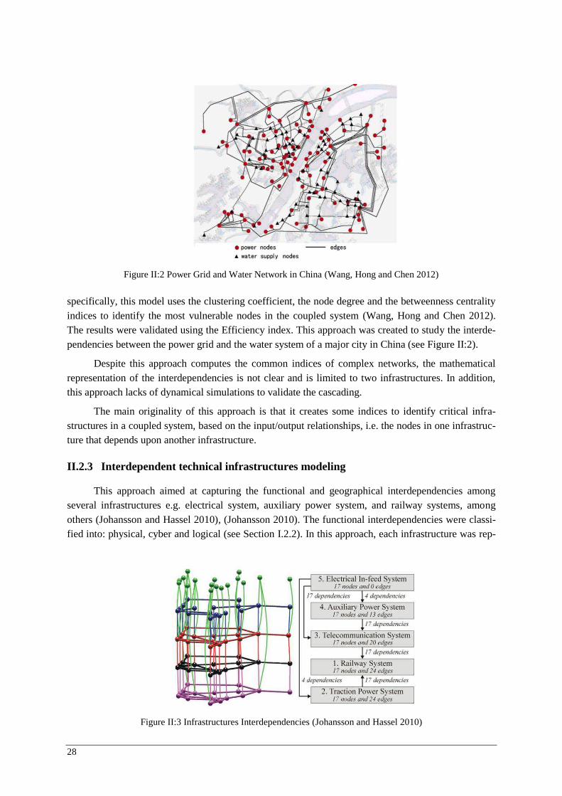
28
specifically, this model uses the clustering coefficient, the node degree and the betweenness centrality indices to identify the most vulnerable nodes in the coupled system (Wang, Hong and Chen 2012). The results were validated using the Efficiency index. This approach was created to study the interde-pendencies between the power grid and the water system of a major city in China (see Figure II :2).
Despite this approach computes the common indices of complex networks, the mathematical representation of the interdependencies is not clear and is limited to two infrastructures. In addition, this approach lacks of dynamical simulations to validate the cascading.
The main originality of this approach is that it creates some indices to identify critical infra-structures in a coupled system, based on the input/output relationships, i.e. the nodes in one infrastruc-ture that depends upon another infrastructure.
II.2.3 Interdependent technical infrastructures modeling
This approach aimed at capturing the functional and geographical interdependencies among several infrastructures e.g. electrical system, auxiliary power system, and railway systems, among others (Johansson and Hassel 2010), (Johansson 2010). The functional interdependencies were classi-fied into: physical, cyber and logical (see Section I.2.2). In this approach, each infrastructure was rep-
Figure II :2 Power Grid and Water Network in China (Wang, Hong and Chen 2012)
Figure II :3 Infrastructures Interdependencies (Johansson and Hassel 2010)
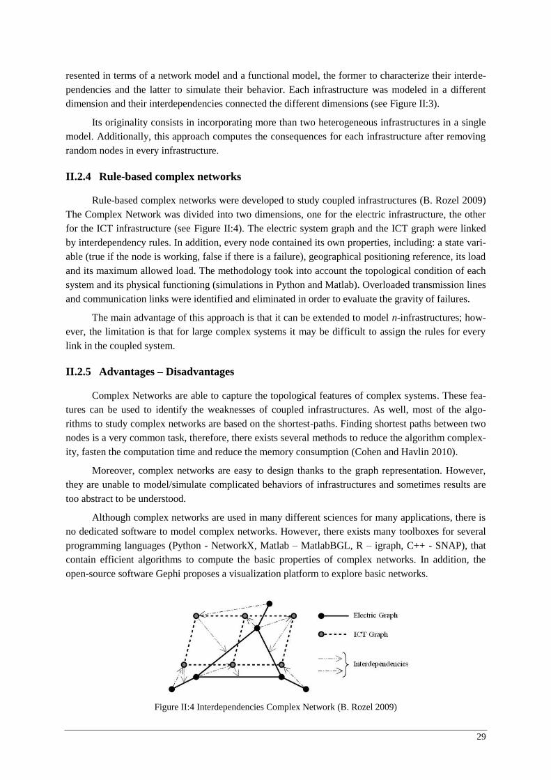
29
resented in terms of a network model and a functional model, the former to characterize their interde-pendencies and the latter to simulate their behavior. Each infrastructure was modeled in a different dimension and their interdependencies connected the different dimensions (see Figure II :3).
Its originality consists in incorporating more than two heterogeneous infrastructures in a single model. Additionally, this approach computes the consequences for each infrastructure after removing random nodes in every infrastructure.
II.2.4 Rule-based complex networks
Rule-based complex networks were developed to study coupled infrastructures (B. Rozel 2009) The Complex Network was divided into two dimensions, one for the electric infrastructure, the other for the ICT infrastructure (see Figure II :4). The electric system graph and the ICT graph were linked by interdependency rules. In addition, every node contained its own properties, including: a state vari-able (true if the node is working, false if there is a failure), geographical positioning reference, its load and its maximum allowed load. The methodology took into account the topological condition of each system and its physical functioning (simulations in Python and Matlab). Overloaded transmission lines and communication links were identified and eliminated in order to evaluate the gravity of failures.
The main advantage of this approach is that it can be extended to model n-infrastructures; how-ever, the limitation is that for large complex systems it may be difficult to assign the rules for every link in the coupled system.
II.2.5 Advantages – Disadvantages
Complex Networks are able to capture the topological features of complex systems. These fea-tures can be used to identify the weaknesses of coupled infrastructures. As well, most of the algo-rithms to study complex networks are based on the shortest-paths. Finding shortest paths between two nodes is a very common task, therefore, there exists several methods to reduce the algorithm complex-ity, fasten the computation time and reduce the memory consumption (Cohen and Havlin 2010).
Moreover, complex networks are easy to design thanks to the graph representation. However, they are unable to model/simulate complicated behaviors of infrastructures and sometimes results are too abstract to be understood.
Although complex networks are used in many different sciences for many applications, there is no dedicated software to model complex networks. However, there exists many toolboxes for several programming languages (Python - NetworkX, Matlab – MatlabBGL, R – igraph, C++ - SNAP), that contain efficient algorithms to compute the basic properties of complex networks. In addition, the open-source software Gephi proposes a visualization platform to explore basic networks.
Figure II :4 Interdependencies Complex Network (B. Rozel 2009)
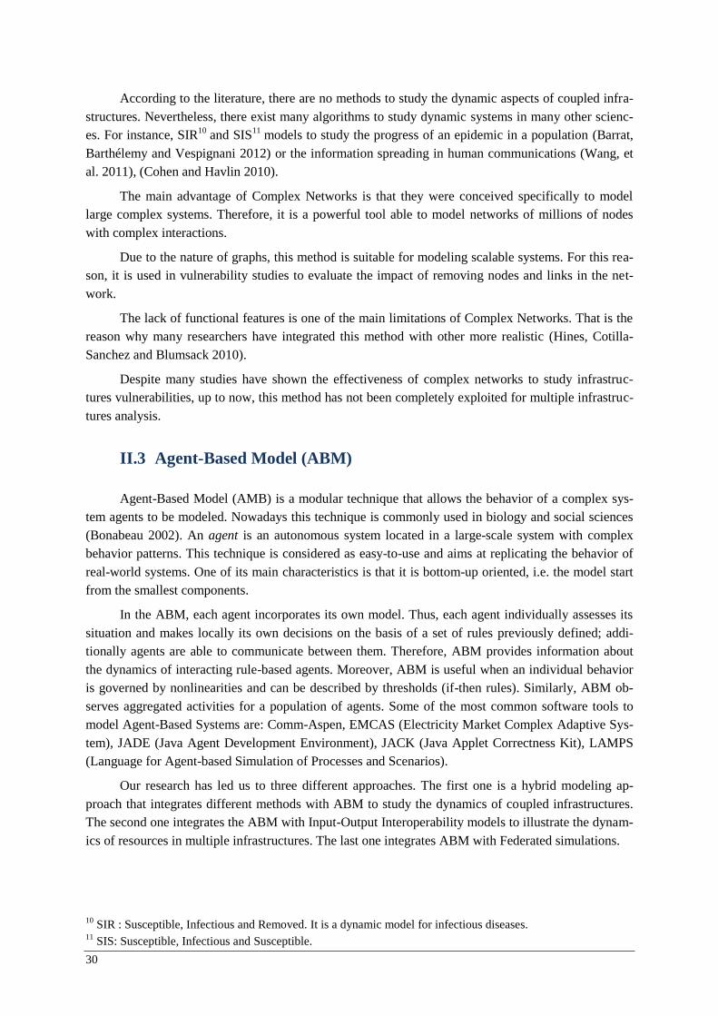
30
According to the literature, there are no methods to study the dynamic aspects of coupled infra-structures. Nevertheless, there exist many algorithms to study dynamic systems in many other scienc-es. For instance, SIR10 and SIS11 models to study the progress of an epidemic in a population (Barrat, Barthélemy and Vespignani 2012) or the information spreading in human communications (Wang, et al. 2011), (Cohen and Havlin 2010).
The main advantage of Complex Networks is that they were conceived specifically to model large complex systems. Therefore, it is a powerful tool able to model networks of millions of nodes with complex interactions.
Due to the nature of graphs, this method is suitable for modeling scalable systems. For this rea-son, it is used in vulnerability studies to evaluate the impact of removing nodes and links in the net-work.
The lack of functional features is one of the main limitations of Complex Networks. That is the reason why many researchers have integrated this method with other more realistic (Hines, Cotilla-Sanchez and Blumsack 2010).
Despite many studies have shown the effectiveness of complex networks to study infrastruc-tures vulnerabilities, up to now, this method has not been completely exploited for multiple infrastruc-tures analysis.
II.3 Agent-Based Model (ABM)
Agent-Based Model (AMB) is a modular technique that allows the behavior of a complex sys-tem agents to be modeled. Nowadays this technique is commonly used in biology and social sciences (Bonabeau 2002). An agent is an autonomous system located in a large-scale system with complex behavior patterns. This technique is considered as easy-to-use and aims at replicating the behavior of real-world systems. One of its main characteristics is that it is bottom-up oriented, i.e. the model start from the smallest components.
In the ABM, each agent incorporates its own model. Thus, each agent individually assesses its situation and makes locally its own decisions on the basis of a set of rules previously defined; addi-tionally agents are able to communicate between them. Therefore, ABM provides information about the dynamics of interacting rule-based agents. Moreover, ABM is useful when an individual behavior is governed by nonlinearities and can be described by thresholds (if-then rules). Similarly, ABM ob-serves aggregated activities for a population of agents. Some of the most common software tools to model Agent-Based Systems are: Comm-Aspen, EMCAS (Electricity Market Complex Adaptive Sys-tem), JADE (Java Agent Development Environment), JACK (Java Applet Correctness Kit), LAMPS (Language for Agent-based Simulation of Processes and Scenarios).
Our research has led us to three different approaches. The first one is a hybrid modeling ap-proach that integrates different methods with ABM to study the dynamics of coupled infrastructures. The second one integrates the ABM with Input-Output Interoperability models to illustrate the dynam-ics of resources in multiple infrastructures. The last one integrates ABM with Federated simulations.
10 SIR : Susceptible, Infectious and Removed. It is a dynamic model for infectious diseases. 11 SIS: Susceptible, Infectious and Susceptible.
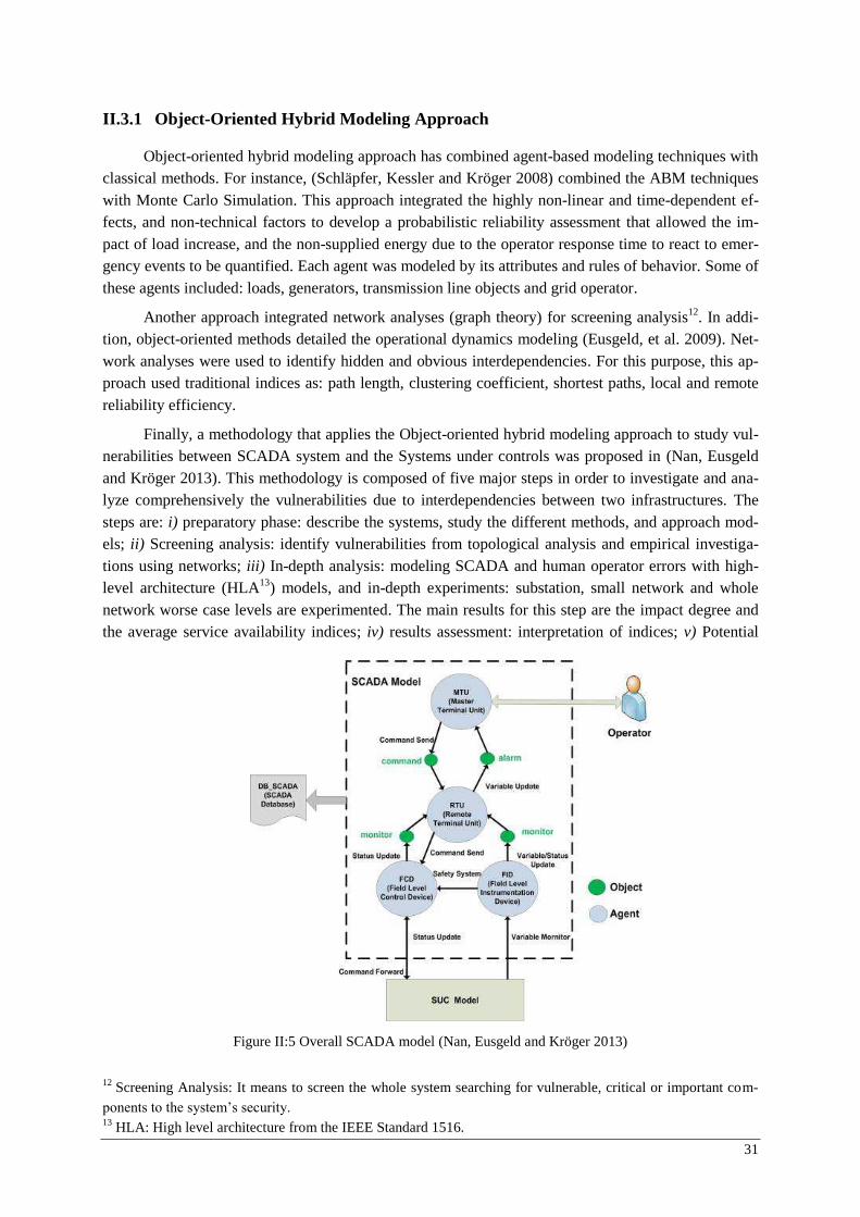
31
II.3.1 Object-Oriented Hybrid Modeling Approach
Object-oriented hybrid modeling approach has combined agent-based modeling techniques with classical methods. For instance, (Schläpfer, Kessler and Kröger 2008) combined the ABM techniques with Monte Carlo Simulation. This approach integrated the highly non-linear and time-dependent ef-fects, and non-technical factors to develop a probabilistic reliability assessment that allowed the im-pact of load increase, and the non-supplied energy due to the operator response time to react to emer-gency events to be quantified. Each agent was modeled by its attributes and rules of behavior. Some of these agents included: loads, generators, transmission line objects and grid operator.
Another approach integrated network analyses (graph theory) for screening analysis12. In addi-tion, object-oriented methods detailed the operational dynamics modeling (Eusgeld, et al. 2009). Net-work analyses were used to identify hidden and obvious interdependencies. For this purpose, this ap-proach used traditional indices as: path length, clustering coefficient, shortest paths, local and remote reliability efficiency.
Finally, a methodology that applies the Object-oriented hybrid modeling approach to study vul-nerabilities between SCADA system and the Systems under controls was proposed in (Nan, Eusgeld and Kröger 2013). This methodology is composed of five major steps in order to investigate and ana-lyze comprehensively the vulnerabilities due to interdependencies between two infrastructures. The steps are: i) preparatory phase: describe the systems, study the different methods, and approach mod-els; ii) Screening analysis: identify vulnerabilities from topological analysis and empirical investiga-tions using networks; iii) In-depth analysis: modeling SCADA and human operator errors with high-level architecture (HLA13) models, and in-depth experiments: substation, small network and whole network worse case levels are experimented. The main results for this step are the impact degree and the average service availability indices; iv) results assessment: interpretation of indices; v) Potential
12 Screening Analysis: It means to screen the whole system searching for vulnerable, critical or important com-ponents to the system’s security. 13 HLA: High level architecture from the IEEE Standard 1516.
Figure II :5 Overall SCADA model (Nan, Eusgeld and Kröger 2013)
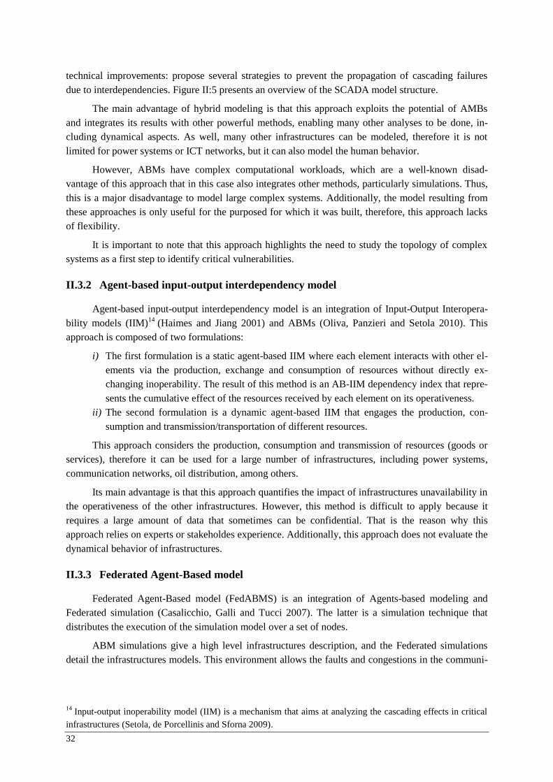
32
technical improvements: propose several strategies to prevent the propagation of cascading failures due to interdependencies. Figure II :5 presents an overview of the SCADA model structure.
The main advantage of hybrid modeling is that this approach exploits the potential of AMBs and integrates its results with other powerful methods, enabling many other analyses to be done, in-cluding dynamical aspects. As well, many other infrastructures can be modeled, therefore it is not limited for power systems or ICT networks, but it can also model the human behavior.
However, ABMs have complex computational workloads, which are a well-known disad-vantage of this approach that in this case also integrates other methods, particularly simulations. Thus, this is a major disadvantage to model large complex systems. Additionally, the model resulting from these approaches is only useful for the purposed for which it was built, therefore, this approach lacks of flexibility.
It is important to note that this approach highlights the need to study the topology of complex systems as a first step to identify critical vulnerabilities.
II.3.2 Agent-based input-output interdependency model
Agent-based input-output interdependency model is an integration of Input-Output Interopera-bility models (IIM)14 (Haimes and Jiang 2001) and ABMs (Oliva, Panzieri and Setola 2010). This approach is composed of two formulations:
i) The first formulation is a static agent-based IIM where each element interacts with other el-ements via the production, exchange and consumption of resources without directly ex-changing inoperability. The result of this method is an AB-IIM dependency index that repre-sents the cumulative effect of the resources received by each element on its operativeness.
ii) The second formulation is a dynamic agent-based IIM that engages the production, con-sumption and transmission/transportation of different resources.
This approach considers the production, consumption and transmission of resources (goods or services), therefore it can be used for a large number of infrastructures, including power systems, communication networks, oil distribution, among others.
Its main advantage is that this approach quantifies the impact of infrastructures unavailability in the operativeness of the other infrastructures. However, this method is difficult to apply because it requires a large amount of data that sometimes can be confidential. That is the reason why this approach relies on experts or stakeholdes experience. Additionally, this approach does not evaluate the dynamical behavior of infrastructures.
II.3.3 Federated Agent-Based model
Federated Agent-Based model (FedABMS) is an integration of Agents-based modeling and Federated simulation (Casalicchio, Galli and Tucci 2007). The latter is a simulation technique that distributes the execution of the simulation model over a set of nodes.
ABM simulations give a high level infrastructures description, and the Federated simulations detail the infrastructures models. This environment allows the faults and congestions in the communi-
14 Input-output inoperability model (IIM) is a mechanism that aims at analyzing the cascading effects in critical infrastructures (Setola, de Porcellinis and Sforna 2009).
33
cation network to be simulated. The main indices obtained from the simulation were: time needed to resolve the crisis, time to rescue a wounded agent, number of rescued wounded agents, number of dead wounded agents, among others.
Further approaches included macro and micro agent-based modeling and simulation (Casalicchio, Galli and Tucci 2010).
The macro agent-based modeling and simulation: represents each system as a single agent that offers and consumes services. Each system was simulated in a specific sector simulator. Each simulator shared the status and the services that it was providing or it needed. This ar-chitecture was implemented using FedABMS.
The micro agent-based modeling and simulation: considers every single component or asset in each infrastructure to simulate the behavior of the whole system. In this simulation, every component was an agent.
These simulations were used to study transportation systems. But it enables as well the study of catastrophic scenarios in power systems and communication networks.
The main disadvantage of this approach is that more than a modeling approach, it is a simula-tion tool that uses Agent-based modeling. Therefore, many parameters are needed to each infrastruc-ture and parallel simulations are needed to cope with the study of multiple coupled infrastructures.
However, these simulation approaches describe the dynamic of coupled infrastructures and are able to handle more than 3 infrastructures at the same time.
II.3.4 Advantages - Disadvantages
Agent-based models have been extensively used to model coupled infrastructures, as shown in this section. Particularly, this model has been used to complement other methods, such as Federated models, Monte Carlo simulations or functional simulations.
The main disadvantage of ABM is that requires parallel processing in order to model large and complex systems and to reduce the computational time needed to study these systems. However, this method has many advantages that highlight its usefulness.
ABM is able to model many different heterogeneous infrastructures and can include different factors such as natural hazards, institutional weaknesses, human behavior, physical laws, or security related issues. As well, it can include reliability aspects for Electric Power Systems and ICTs.
Because ABM has been widely used, there exist many robust platforms in multiples program-ming languages to visualize and analyze ABMs. Moreover, AMBs include time-dependent nonlinear phenomena into the simulation. As a result of this, ABMs demonstrates a close adherence to the reality of the coupled processes involved in simulations
The bottom-up oriented modeling allows large complex systems to be modeled, including many parameters from the smallest component to the whole system behavior. However, sometimes it could be difficult to model large complex systems, because the model may require a large number of param-eters to improve the models accuracy.
The presented approaches reveal that ABM needs to be complemented with other methods in order to consider the whole behavior of coupled infrastructures. One of these proposed methods was the ‘Complex Network theory’, which can improve the screening analysis to identify weaknesses in coupled heterogeneous infrastructures.
34
II.4 Bayesian Networks (BN)
A Bayesian Network is a compact graphical representation that supports systems modeling, in-cluding random events, and it is based on the Bayes theorem (allows calculating the a posteriori prob-ability as a function of a priori probabilities) (Birolini 2007).
Bayesian Network’s nodes represent the propositional variables, and links represent the causal dependencies among the nodes, these dependencies are quantified by conditional probabilities (Pearl and Russell 2003).
Two main methods were identified in the literature, the first one evaluates the cause-effect in-terdependencies and the second one models the dynamics in coupled infrastructures.
II.4.1 Cause-Effect interdependencies
The structure of Bayesian Networks was used to illustrate the cause-effect interactions between ICT infrastructure and Power Systems (Tranchita, Hadjsaid, et al. 2010). This method mimicked cau-sality and inference presented in both infrastructures in order to assess the power system risk as a re-sult of cyber terrorism. The model was divided into four main phases (Tranchita 2008):
Identify the ICT attacking motivation: Determine whether the attack is due to a political or religious situation, or to a terrorist activity. The motivation was divided into High, Medium and Low level.
Identify vulnerable resources: It is important to detect the type of perpetrator, which could be either: an insider employee, an insider service provider, an outsider former-insider, an outsider professional hacker, or an outsider cybercriminal. The information availability was divided into: enough, regular or low, this variable is important since a terrorist with enough information to attack is more dangerous for critical infrastructures.
Quantify assets’ vulnerability: It was evaluated according to the geographical situation and to the physical protection of assets. This phase studied software, hardware and configuration vulnerabilities. The vulnerabilities were divided into: Highly, averagely and lowly vulnera-ble. This phase was supported by a power flow analysis to study the system response to N-1 contingencies.
Determine the consequences for the power system operation: The Power system damage was evaluated and classified in different levels of severity: low, medium, high and cata-strophic. The possible functions executed to attack the infrastructures were evaluated, in-cluding: protection, control, monitoring, measurements and management.
This approach can be used to study power transmission and distribution systems with different attack scenario without considering the dynamic aspects. It can be used to quantify the consequences of targeted attacks to certain assets and to classify these consequences in different gravity levels.
Even if the application of this approach is easy, taking into account the diversity of tools availa-ble, this method relies on information that is not always available and most of the times have to be obtained from experts and operators experience and knowledge.
On the other hand, usually, the computing time needed to compute this method is very short even if it is dealing with multiple infrastructures. Additionally, this approach can consider the impact of many different heterogeneous infrastructures in the risk analysis of power systems; however, it de-pends on probabilistic information that is not always reliable and the results will be focused in only

35
one infrastructure.
II.4.2 Dynamic Bayesian Networks
The Dynamic Bayesian Network formalism was used to model critical infrastructures (Di Giorgio and Liberati 2012). The analysis was divided into three levels: atomic event level, propagation level and services level. Atomic level is related to the association of random variables to possible ad-verse events. Propagation level models the interdependencies among and within infrastructures, some of the subsystems involved are: electric transmission network, SCADA feeder, and SCADA system. Services level involves the operators and control centers. A graphical representation of the Dynamic Bayesian Network is presented in Figure II :6.
The proposed methodology was divided into the following steps:
Identification of relevant services.
Identification of main devices and functions needed to deliver the services to the end-used.
Identification of common devices among different services.
Localization of devices in the grid topology to study the geographical interdependencies.
Identification of random variables of possible events in the atomic level and evaluation of possible effects on propagation level.
Study of temporal interdependencies in the Dynamic Bayesian Network.
Three different analyses can be performed based on this approach: reliability study, adverse event spreading and forecasting. Nevertheless, the main advantage of this method is that it is able to model different failures modes and allows the impact of those failures to be quantified, taking into account dynamic simulations. Additionally, this approach can be scalable to larger infrastructures. However, the dynamic simulations are not continuous, but static model assessments in discrete time steps.
Another disadvantage of this approach is that it relies on data from literature, historical events or domain-experts opinion. Therefore, the accuracy of results depends on the parameters that it use, which may not be very reliable. In fact, in order to improve the accuracy, this approach needs a large number of parameters, but these parameters can increase the computational complexity.
Figure II :6 Overall Dynamic Bayesian Network (Di Giorgio and Liberati 2012)
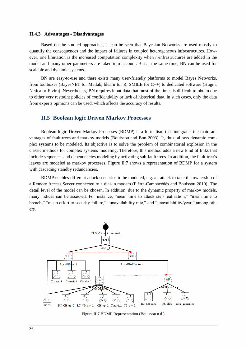
36
II.4.3 Advantages - Disadvantages
Based on the studied approaches, it can be seen that Bayesian Networks are used mostly to quantify the consequences and the impact of failures in coupled heterogeneous infrastructures. How-ever, one limitation is the increased computation complexity when n-infrastructures are added in the model and many other parameters are taken into account. But at the same time, BN can be used for scalable and dynamic systems.
BN are easy-to-use and there exists many user-friendly platforms to model Bayes Networks, from toolboxes (BayesNET for Matlab, blearn for R, SMILE for C++) to dedicated software (Hugin, Netica or Elvira). Nevertheless, BN requires input data that most of the times is difficult to obtain due to either very restraint policies of confidentiality or lack of historical data. In such cases, only the data from experts opinions can be used, which affects the accuracy of results.
II.5 Boolean logic Driven Markov Processes
Boolean logic Driven Markov Processes (BDMP) is a formalism that integrates the main ad-vantages of fault-trees and markov models (Bouissou and Bon 2003). It, thus, allows dynamic com-plex systems to be modeled. Its objective is to solve the problem of combinatorial explosion in the classic methods for complex systems modeling. Therefore, this method adds a new kind of links that include sequences and dependencies modeling by activating sub-fault trees. In addition, the fault-tree’s leaves are modeled as markov processes. Figure II :7 shows a representation of BDMP for a system with cascading standby redundancies.
BDMP enables different attack scenarios to be modeled, e.g. an attack to take the ownership of a Remote Access Server connected to a dial-in modem (Piètre-Cambacédès and Bouissou 2010). The detail level of the model can be chosen. In addition, due to the dynamic property of markov models, many indices can be assessed. For instance, “mean time to attack step realization,” “mean time to breach,” “mean effort to security failure,” “unavailability rate,” and “unavailability/year,” among oth-ers.
Figure II :7 BDMP Representation (Bouisson n.d.)
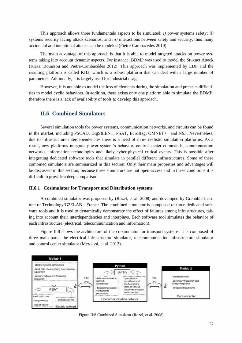
37
This approach allows three fundamentals aspects to be simulated: i) power systems safety; ii) systems security facing attack scenarios; and iii) interactions between safety and security, thus many accidental and intentional attacks can be modeled (Piètre-Cambacédès 2010).
The main advantage of this approach is that it is able to model targeted attacks on power sys-tems taking into account dynamic aspects. For instance, BDMP was used to model the Stuxnet Attack (Kriaa, Bouissou and Piètre-Cambacédès 2012). This approach was implemented by EDF and the resulting platform is called KB3, which is a robust platform that can deal with a large number of parameters. Aditionally, it is largely used for industrial usage.
However, it is not able to model the loss of elements during the simulation and presents difficul-ties to model cyclic behaviors. In addition, there exists only one platform able to simulate the BDMP, therefore there is a lack of availability of tools to develop this approach.
II.6 Combined Simulators
Several simulation tools for power systems, communication networks, and circuits can be found in the market, including PSCAD, DigSILENT, PSAT, Eurostag, OMNET++ and NS3. Nevertheless, due to infrastructure interdependencies there is a need of more realistic simulation platforms. As a result, new platforms integrate power system’s behavior, control center commands, communication networks, information technologies and likely cyber-physical critical events. This is possible after integrating dedicated software tools that simulate in parallel different infrastructures. Some of these combined simulators are summarized in this section. Only their main properties and advantages will be discussed in this section, because these simulators are not open-access and in these conditions it is difficult to provide a deep comparison.
II.6.1 Cosimulator for Transport and Distribution systems
A combined simulator was proposed by (Rozel, et al. 2008) and developed by Grenoble Insti-tute of Technology/G2ELAB - France. The combined simulator is composed of three dedicated soft-ware tools and it is used to dynamically demonstrate the effect of failures among infrastructures, tak-ing into account their interdependencies and interplays. Each software tool simulates the behavior of each infrastructure (electrical, telecommunication and information).
Figure II :8 shows the architecture of the co-simulator for transport systems. It is composed of three main parts: the electrical infrastructure simulator, telecommunication infrastructure simulator and control center simulator (Merdassi, et al. 2012).
Figure II :8 Combined Simulator (Rozel, et al. 2008)
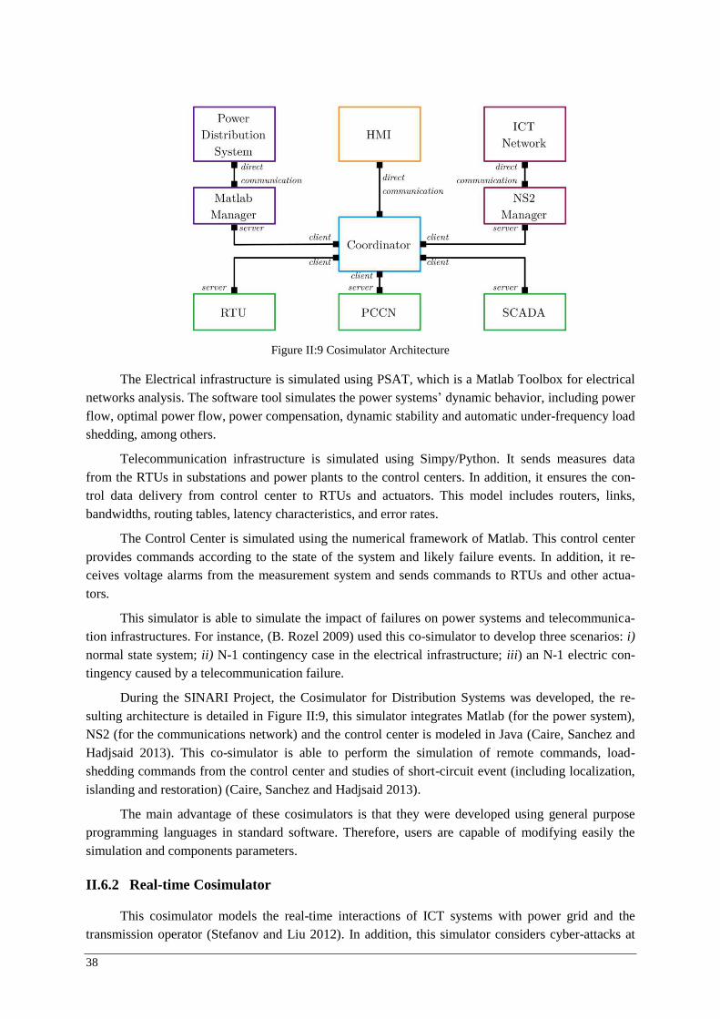
38
The Electrical infrastructure is simulated using PSAT, which is a Matlab Toolbox for electrical networks analysis. The software tool simulates the power systems’ dynamic behavior, including power flow, optimal power flow, power compensation, dynamic stability and automatic under-frequency load shedding, among others.
Telecommunication infrastructure is simulated using Simpy/Python. It sends measures data from the RTUs in substations and power plants to the control centers. In addition, it ensures the con-trol data delivery from control center to RTUs and actuators. This model includes routers, links, bandwidths, routing tables, latency characteristics, and error rates.
The Control Center is simulated using the numerical framework of Matlab. This control center provides commands according to the state of the system and likely failure events. In addition, it re-ceives voltage alarms from the measurement system and sends commands to RTUs and other actua-tors.
This simulator is able to simulate the impact of failures on power systems and telecommunica-tion infrastructures. For instance, (B. Rozel 2009) used this co-simulator to develop three scenarios: i) normal state system; ii) N-1 contingency case in the electrical infrastructure; iii ) an N-1 electric con-tingency caused by a telecommunication failure.
During the SINARI Project, the Cosimulator for Distribution Systems was developed, the re-sulting architecture is detailed in Figure II :9, this simulator integrates Matlab (for the power system), NS2 (for the communications network) and the control center is modeled in Java (Caire, Sanchez and Hadjsaid 2013). This co-simulator is able to perform the simulation of remote commands, load-shedding commands from the control center and studies of short-circuit event (including localization, islanding and restoration) (Caire, Sanchez and Hadjsaid 2013).
The main advantage of these cosimulators is that they were developed using general purpose programming languages in standard software. Therefore, users are capable of modifying easily the simulation and components parameters.
II.6.2 Real-time Cosimulator
This cosimulator models the real-time interactions of ICT systems with power grid and the transmission operator (Stefanov and Liu 2012). In addition, this simulator considers cyber-attacks at
Figure II :9 Cosimulator Architecture
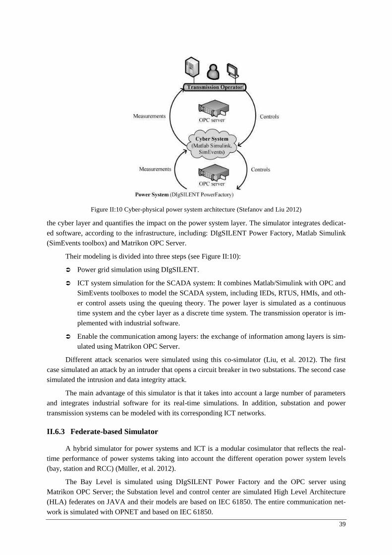
39
the cyber layer and quantifies the impact on the power system layer. The simulator integrates dedicat-ed software, according to the infrastructure, including: DIgSILENT Power Factory, Matlab Simulink (SimEvents toolbox) and Matrikon OPC Server.
Their modeling is divided into three steps (see Figure II :10):
Power grid simulation using DIgSILENT.
ICT system simulation for the SCADA system: It combines Matlab/Simulink with OPC and SimEvents toolboxes to model the SCADA system, including IEDs, RTUS, HMIs, and oth-er control assets using the queuing theory. The power layer is simulated as a continuous time system and the cyber layer as a discrete time system. The transmission operator is im-plemented with industrial software.
Enable the communication among layers: the exchange of information among layers is sim-ulated using Matrikon OPC Server.
Different attack scenarios were simulated using this co-simulator (Liu, et al. 2012). The first case simulated an attack by an intruder that opens a circuit breaker in two substations. The second case simulated the intrusion and data integrity attack.
The main advantage of this simulator is that it takes into account a large number of parameters and integrates industrial software for its real-time simulations. In addition, substation and power transmission systems can be modeled with its corresponding ICT networks.
II.6.3 Federate-based Simulator
A hybrid simulator for power systems and ICT is a modular cosimulator that reflects the real-time performance of power systems taking into account the different operation power system levels (bay, station and RCC) (Müller, et al. 2012).
The Bay Level is simulated using DIgSILENT Power Factory and the OPC server using Matrikon OPC Server; the Substation level and control center are simulated High Level Architecture (HLA) federates on JAVA and their models are based on IEC 61850. The entire communication net-work is simulated with OPNET and based on IEC 61850.
Figure II :10 Cyber-physical power system architecture (Stefanov and Liu 2012)
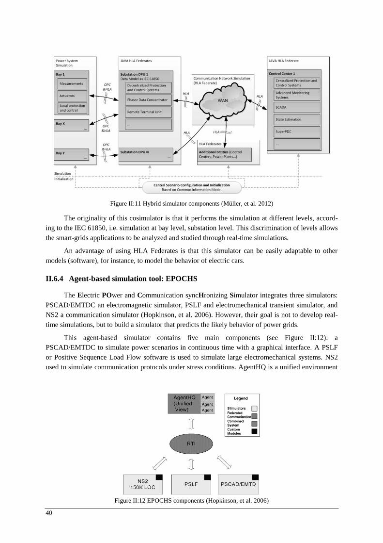
40
The originality of this cosimulator is that it performs the simulation at different levels, accord-ing to the IEC 61850, i.e. simulation at bay level, substation level. This discrimination of levels allows the smart-grids applications to be analyzed and studied through real-time simulations.
An advantage of using HLA Federates is that this simulator can be easily adaptable to other models (software), for instance, to model the behavior of electric cars.
II.6.4 Agent-based simulation tool: EPOCHS
The Electric POwer and Communication syncHronizing Simulator integrates three simulators: PSCAD/EMTDC an electromagnetic simulator, PSLF and electromechanical transient simulator, and NS2 a communication simulator (Hopkinson, et al. 2006). However, their goal is not to develop real-time simulations, but to build a simulator that predicts the likely behavior of power grids.
This agent-based simulator contains five main components (see Figure II :12): a PSCAD/EMTDC to simulate power scenarios in continuous time with a graphical interface. A PSLF or Positive Sequence Load Flow software is used to simulate large electromechanical systems. NS2 used to simulate communication protocols under stress conditions. AgentHQ is a unified environment
Figure II :11 Hybrid simulator components (Müller, et al. 2012)
Figure II :12 EPOCHS components (Hopkinson, et al. 2006)
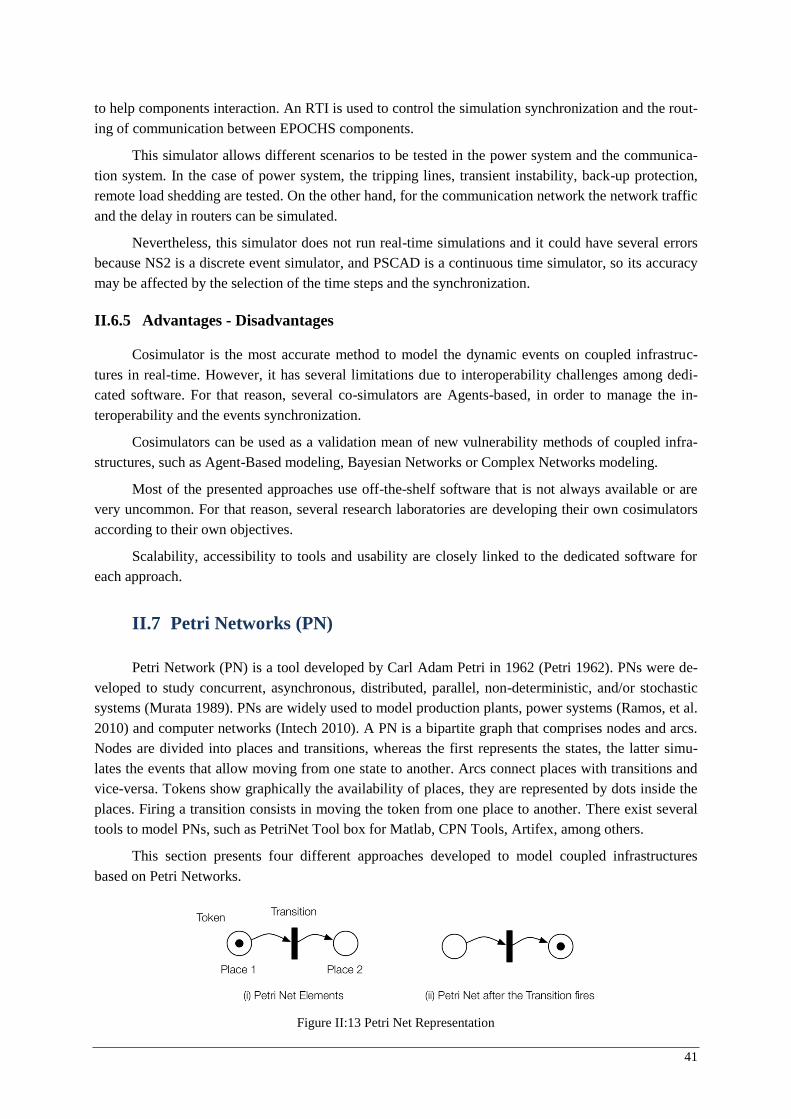
41
to help components interaction. An RTI is used to control the simulation synchronization and the rout-ing of communication between EPOCHS components.
This simulator allows different scenarios to be tested in the power system and the communica-tion system. In the case of power system, the tripping lines, transient instability, back-up protection, remote load shedding are tested. On the other hand, for the communication network the network traffic and the delay in routers can be simulated.
Nevertheless, this simulator does not run real-time simulations and it could have several errors because NS2 is a discrete event simulator, and PSCAD is a continuous time simulator, so its accuracy may be affected by the selection of the time steps and the synchronization.
II.6.5 Advantages - Disadvantages
Cosimulator is the most accurate method to model the dynamic events on coupled infrastruc-tures in real-time. However, it has several limitations due to interoperability challenges among dedi-cated software. For that reason, several co-simulators are Agents-based, in order to manage the in-teroperability and the events synchronization.
Cosimulators can be used as a validation mean of new vulnerability methods of coupled infra-structures, such as Agent-Based modeling, Bayesian Networks or Complex Networks modeling.
Most of the presented approaches use off-the-shelf software that is not always available or are very uncommon. For that reason, several research laboratories are developing their own cosimulators according to their own objectives.
Scalability, accessibility to tools and usability are closely linked to the dedicated software for each approach.
II.7 Petri Networks (PN)
Petri Network (PN) is a tool developed by Carl Adam Petri in 1962 (Petri 1962). PNs were de-veloped to study concurrent, asynchronous, distributed, parallel, non-deterministic, and/or stochastic systems (Murata 1989). PNs are widely used to model production plants, power systems (Ramos, et al. 2010) and computer networks (Intech 2010). A PN is a bipartite graph that comprises nodes and arcs. Nodes are divided into places and transitions, whereas the first represents the states, the latter simu-lates the events that allow moving from one state to another. Arcs connect places with transitions and vice-versa. Tokens show graphically the availability of places, they are represented by dots inside the places. Firing a transition consists in moving the token from one place to another. There exist several tools to model PNs, such as PetriNet Tool box for Matlab, CPN Tools, Artifex, among others.
This section presents four different approaches developed to model coupled infrastructures based on Petri Networks.
Figure II :13 Petri Net Representation
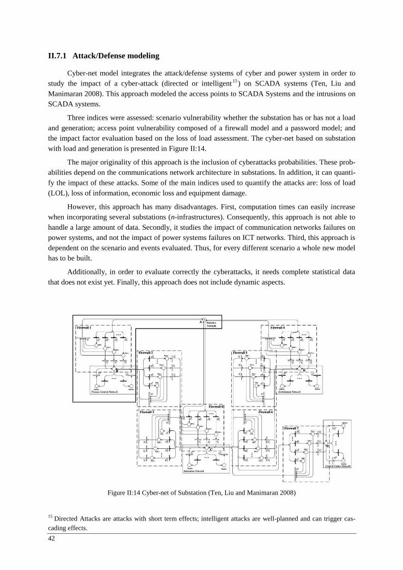
42
II.7.1 Attack/Defense modeling
Cyber-net model integrates the attack/defense systems of cyber and power system in order to study the impact of a cyber-attack (directed or intelligent15) on SCADA systems (Ten, Liu and Manimaran 2008). This approach modeled the access points to SCADA Systems and the intrusions on SCADA systems.
Three indices were assessed: scenario vulnerability whether the substation has or has not a load and generation; access point vulnerability composed of a firewall model and a password model; and the impact factor evaluation based on the loss of load assessment. The cyber-net based on substation with load and generation is presented in Figure II :14.
The major originality of this approach is the inclusion of cyberattacks probabilities. These prob-abilities depend on the communications network architecture in substations. In addition, it can quanti-fy the impact of these attacks. Some of the main indices used to quantify the attacks are: loss of load (LOL), loss of information, economic loss and equipment damage.
However, this approach has many disadvantages. First, computation times can easily increase when incorporating several substations (n-infrastructures). Consequently, this approach is not able to handle a large amount of data. Secondly, it studies the impact of communication networks failures on power systems, and not the impact of power systems failures on ICT networks. Third, this approach is dependent on the scenario and events evaluated. Thus, for every different scenario a whole new model has to be built.
Additionally, in order to evaluate correctly the cyberattacks, it needs complete statistical data that does not exist yet. Finally, this approach does not include dynamic aspects.
15 Directed Attacks are attacks with short term effects; intelligent attacks are well-planned and can trigger cas-cading effects.
Figure II :14 Cyber-net of Substation (Ten, Liu and Manimaran 2008)
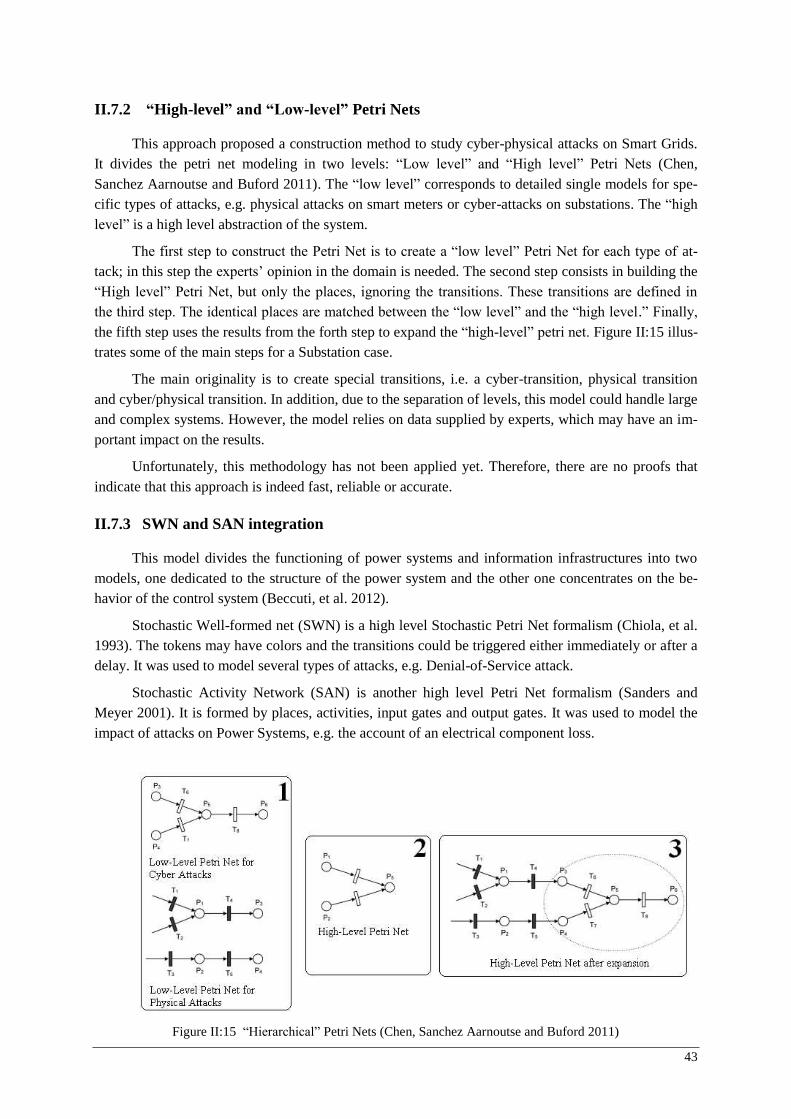
43
II.7.2 “High-level” and “Low-level” Petri Nets
This approach proposed a construction method to study cyber-physical attacks on Smart Grids. It divides the petri net modeling in two levels: “Low level” and “High level” Petri Nets (Chen, Sanchez Aarnoutse and Buford 2011). The “low level” corresponds to detailed single models for spe-cific types of attacks, e.g. physical attacks on smart meters or cyber-attacks on substations. The “high level” is a high level abstraction of the system.
The first step to construct the Petri Net is to create a “low level” Petri Net for each type of at-tack; in this step the experts’ opinion in the domain is needed. The second step consists in building the “High level” Petri Net, but only the places, ignoring the transitions. These transitions are defined in the third step. The identical places are matched between the “low level” and the “high level.” Finally, the fifth step uses the results from the forth step to expand the “high-level” petri net. Figure II :15 illus-trates some of the main steps for a Substation case.
The main originality is to create special transitions, i.e. a cyber-transition, physical transition and cyber/physical transition. In addition, due to the separation of levels, this model could handle large and complex systems. However, the model relies on data supplied by experts, which may have an im-portant impact on the results.
Unfortunately, this methodology has not been applied yet. Therefore, there are no proofs that indicate that this approach is indeed fast, reliable or accurate.
II.7.3 SWN and SAN integration
This model divides the functioning of power systems and information infrastructures into two models, one dedicated to the structure of the power system and the other one concentrates on the be-havior of the control system (Beccuti, et al. 2012).
Stochastic Well-formed net (SWN) is a high level Stochastic Petri Net formalism (Chiola, et al. 1993). The tokens may have colors and the transitions could be triggered either immediately or after a delay. It was used to model several types of attacks, e.g. Denial-of-Service attack.
Stochastic Activity Network (SAN) is another high level Petri Net formalism (Sanders and Meyer 2001). It is formed by places, activities, input gates and output gates. It was used to model the impact of attacks on Power Systems, e.g. the account of an electrical component loss.
Figure II :15 “Hierarchical” Petri Nets (Chen, Sanchez Aarnoutse and Buford 2011)
44
Different performance indices that describe the impact of critical attacks can be created from the integration of both methods. Some of these indices are “Unsatisfied Demand” and “Percentage of Un-satisfied demand.” In addition, many failures can be considered, mainly DoS attacks.
The originality of this method lies in the integration of two high-level formalisms for Petri Nets. This integration allows the consequences of cyberattacks to be quantified using performance indices and taking into account the randomness of failure events in coupled infrastructures. A wide variety of scenarios can be analyzed with this approach, which is agent-based.
The scope of this approach is the study of DoS attacks, including the spread speed and the quan-tification of the dynamic consequences. However, the dynamic aspects are only addressed in discrete time simulations and a combinatorial explosion could limit the ability to model large complex system.
II.7.4 Intrusion detection on Cyber Physical Systems
This approach studies the effect of intrusion detection systems on the reliability of cyber physi-cal systems, e.g. sensors, actuators and control units, in a context wherein energy replenishment is not possible (Mitchell and Chen 2013). This approach is based on stochastic petri nets, which models semi-Markov processes with a state representation.
The main originality is that in this approach, the system’s nodes are modeled as tokens, and not as places. This approach is specialized in intrusion detection and response systems and allows the mean time to failure (MTTF) to be computed, taking into account the cyber-vulnerabilities at different layers.
However it does not take into account the power system dynamics. In fact, it is mostly a com-munication networks security analysis than a multi-infrastructure analysis. In addition, this modeling is exposed to the state explosion problem due to the quantity of tokens needed for large systems.
Also, this method can be used maximum for two coupled infrastructures where one of them is the Communications Network.
II.7.5 Advantages - Disadvantages
Petri Networks are a powerful method to model complex sequential processes. However, many applications and developments have arisen in order to model complex dynamic systems, such as Pow-er Systems and Computer networks.
However, PN were not created to model large systems and its main limitation is the state explo-sion, making it very difficult to use them to model complex coupled heterogeneous infrastructures.
The main advantage of PN is that it can model discrete and continuous time systems, consider-ing stochastic and timed transitions. In addition, thanks to the last developments, petri networks can be used as modules. Nevertheless, the level of maturity for these purposes is still very low.
II.8 Comparison and Conclusion
This chapter provides a comprehensive state-of-the art of modeling approaches and methods to solve the emerging challenges of interdependent coupled infrastructures. As the reader may notice, most of the explored literature is recent. When starting the SINARI project, the Sate-of-the-art that was prepared and published at that time was very different from the one presented in this chapter (see (Merdassi, et al. 2012)).
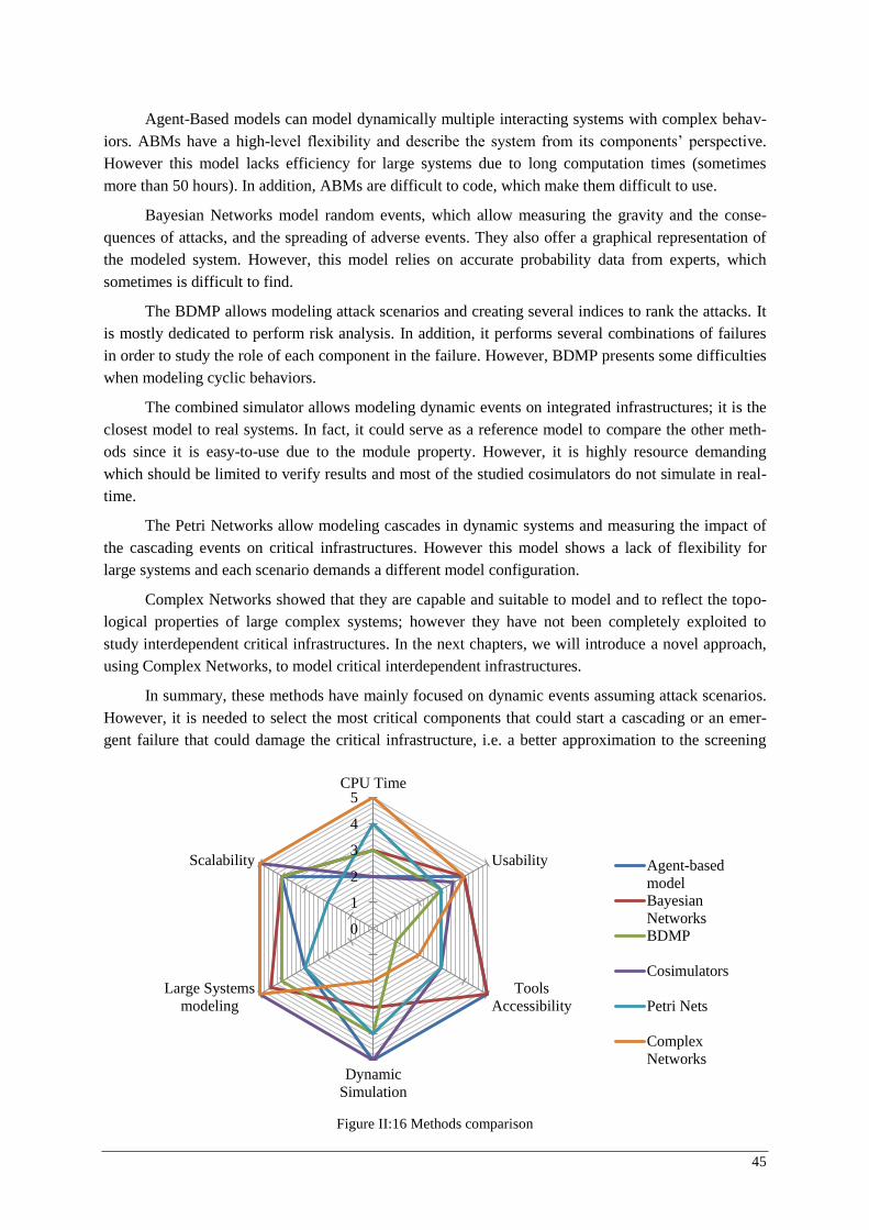
45
Agent-Based models can model dynamically multiple interacting systems with complex behav-iors. ABMs have a high-level flexibility and describe the system from its components’ perspective. However this model lacks efficiency for large systems due to long computation times (sometimes more than 50 hours). In addition, ABMs are difficult to code, which make them difficult to use.
Bayesian Networks model random events, which allow measuring the gravity and the conse-quences of attacks, and the spreading of adverse events. They also offer a graphical representation of the modeled system. However, this model relies on accurate probability data from experts, which sometimes is difficult to find.
The BDMP allows modeling attack scenarios and creating several indices to rank the attacks. It is mostly dedicated to perform risk analysis. In addition, it performs several combinations of failures in order to study the role of each component in the failure. However, BDMP presents some difficulties when modeling cyclic behaviors.
The combined simulator allows modeling dynamic events on integrated infrastructures; it is the closest model to real systems. In fact, it could serve as a reference model to compare the other meth-ods since it is easy-to-use due to the module property. However, it is highly resource demanding which should be limited to verify results and most of the studied cosimulators do not simulate in real-time.
The Petri Networks allow modeling cascades in dynamic systems and measuring the impact of the cascading events on critical infrastructures. However this model shows a lack of flexibility for large systems and each scenario demands a different model configuration.
Complex Networks showed that they are capable and suitable to model and to reflect the topo-logical properties of large complex systems; however they have not been completely exploited to study interdependent critical infrastructures. In the next chapters, we will introduce a novel approach, using Complex Networks, to model critical interdependent infrastructures.
In summary, these methods have mainly focused on dynamic events assuming attack scenarios. However, it is needed to select the most critical components that could start a cascading or an emer-gent failure that could damage the critical infrastructure, i.e. a better approximation to the screening
Figure II :16 Methods comparison
0
1
2
3
4
5CPU Time
Usability
ToolsAccessibility
DynamicSimulation
Large Systemsmodeling
Scalability Agent-basedmodelBayesianNetworksBDMP
Cosimulators
Petri Nets
ComplexNetworks

46
methods. Moreover, the most critical component and weakest elements in the system may emerge from the interface of critical infrastructures. Another disadvantage is that these methods are unsuitable to manage large systems to overcome the state explosion problem and there are still some processing capacity limitations.
A method comparison is not completely possible, due to the unlike objectives of each model. Furthermore, there is not a global model that covers the complex world of interdependencies and vul-nerabilities of Critical infrastructures. Figure II :16 plots a comparative diagram, taking into account six aspects:
CPU time: This aspect describes the computation complexity, the memory and process re-quirement. A grade from 1 to 5, where 1 represents an expensive and slow performance and 5 represents a fast process.
Usability: This aspect joints different characteristics, including the easiness to model and the flexibility to model heterogeneous systems. 1 for a difficult to apply method and 5 for an easy-to-use method.
Tools Accessibility: It evaluates the availability of tools that can compute or simulate heter-ogeneous coupled infrastructures. 1 if there are no available tools and 5 if there are many options.
Dynamic simulations: This aspects gives a grade of 1 if this method is not able to model dynamic aspects (or it have not been applied yet), and 5 if it already considers dynamic events.
Large systems modeling: This aspect reports a grade of 1 if the method is not able to handle large complex systems and 5 if it is completely developed to handle these systems.
Scalability: It considers the ability to change in size or scale, it means, a model can be easily expanded to include other components or parameters without requiring a complete change of the model. A grade of 1 is assigned if it is not possible and a grade of 5 if the model is scalable across a large range of changes.
The grades were assigned taking into consideration the exposed approaches and several state-of-the-art found in the literature, including (Merdassi, et al. 2012), (Kröger and Zio 2011), (Galli 2010), (Ouyang 2013), (Cheminod, Durante and Valenzano 2013).
47
CHAPTER III
Vulnerability and Interdependencies: Modeling
We live in a society exquisitely dependent on science and technology,
in which hardly anyone knows anything about science and technology
Carl Sagan
TABLE OF CONTENTS
III.1 INTRODUCTION .............................................................................................................. 48
III.2 FROM GRAPH THEORY TO COMPLEX NETWORKS ......................................................... 49
III.3 CONCEPTUAL AND THEORETICAL FRAMEWORK ........................................................... 53
III.3.1 Notations of Complex Networks ..................................................................... 53
III.3.1.1 Adjacency Matrix ............................................................................. 53
III.3.1.2 Weight Matrix .................................................................................. 54
III.3.1.3 Path length, Geodesic and Diameter ................................................ 54
III.3.1.4 Node Degree ..................................................................................... 55
III.3.1.5 Betweenness Centrality .................................................................... 55
III.3.1.6 Efficiency ......................................................................................... 57
III.3.2 Eigenspectral Analysis ..................................................................................... 58
III.3.2.1 Spectral Analysis .............................................................................. 58
III.3.2.2 Hilbert Space .................................................................................... 59
III.3.2.3 Hermitian Matrices ........................................................................... 60
III.4 VULNERABILITY AND CRITICALITY ANALYSIS .............................................................. 61
III.4.1 Electricity infrastructure topology analysis ..................................................... 61
III.4.2 The topology-driven Approach ........................................................................ 67
III.4.2.1 Complex-valued Node Degree ......................................................... 68
III.4.2.2 Betweenness Centrality for multi-infrastructures ............................. 69
III.4.2.3 Electrical and ICT Efficiency ........................................................... 70
III.4.2.4 Partial Conclusions ........................................................................... 71
III.4.3 Eigenspectral Analysis ..................................................................................... 72
III.4.3.1 Complex-weighted Adjacency Matrix ............................................. 72
48
III.4.3.2 Complex-valued node degree ........................................................... 73
III.4.3.3 Eigenspectral Centrality ................................................................... 73
III.5 SUMMARY ...................................................................................................................... 75
Abstract
Power systems and ICTs interdependencies request innovative and revolutionary methods, built on new
ideas that aim at identifying weaknesses and critical components that can fail and create many other failures
either by cascading, common-mode or escalating. One possible approach to understand critical infrastructures’ vulnerabilities is to study their topologies and to quantify their physical and cyber interdependencies. This chap-
ter presents an introduction to Complex Networks and proposes two approaches to model coupled infrastruc-
tures’ interdependencies: a topologic-driven approach and an eigensystem analysis. The former evaluates com-
plex-weighted graphs to assess the main topological indices. The latter, evaluates the adjacency matrix as a
Hermitian Matrix in the Hilbert Space to study the Eigenspectral of the coupled system. Few simple examples
are shown to exemplify its use.
III.1 Introduction
Electric Power Systems (EPS) and Information and Communication Technologies (ICTs) reveal strong interdependencies among their components as explored in CHAPTER I. For that reason, many methods and algorithms have been developed to study these interdependencies and to ensure high levels of reliability, availability and security of critical infrastructures. Some of these methods are summarized in the state-of-the-art presented in CHAPTER II. One of the main outcomes in CHAP-TER II is that there is either a need for a strong improvement and upgrade of these methods or a need for a new one. This Chapter aims at solving this challenge using ‘Complex Networks Theory’, consid-ering that a major and critical objective is to identify failure initiating events on interdependent cou-pled infrastructures, i.e. the identification of components that are very likely to initiate a failure.
‘Complex Networks’ (or graph theory) is a very promising method according to different publi-cations (Merdassi, et al. 2012), (Kröger and Zio 2011). In this dissertation, it is strongly believed that the topology of coupled infrastructures influences on their behavior of the whole system. Therefore, the study of the structure of coupled infrastructures may help to understand the way each component affects the function of the whole coupled system. These beliefs are supported by several studies in different sciences. For instance, the study of the WWW topology (Albert, Jeong and Barabasi 2000), the Internet (Yook, Jeong and Barabasi 2002), the cellular networks (Jeong, et al. 2000), among others (Albert and Barabasi 2002).
The final objective of this Chapter is to answer the question: How to construct a common-model for coupled infrastructures, taking into account their topological characteristics, enabling to differenti-ate their own communication patterns (the modes of communication), but at the same time being flex-ible in the way it could be used to study n-infrastructures’ interdependencies.
Power Systems are known to be very robust; the origin of this robustness was identified thanks to the use of complex networks theory. (Barabási and Bonabeu 2003) discovered that most of the complex systems have a scale-free characteristic that increase their robustness against random attacks or random failures. However, the Achilles’ heel of complex systems is that most of them rely on few nodes (called Hubs), it has already been demonstrated that the removal of key hubs generates a general failure of the system (Wang and Guanrong 2003). In the case of Electric Power Systems, it has already been demonstrated that the breakdown of a single targeted components is sufficient to collapse the
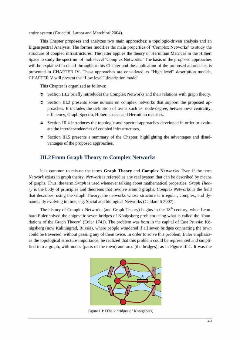
49
entire system (Cruccitti, Latora and Marchiori 2004).
This Chapter proposes and analyzes two main approaches: a topologic-driven analysis and an Eigenspectral Analysis. The former modifies the main properties of ‘Complex Networks’ to study the structure of coupled infrastructures. The latter applies the theory of Hermitian Matrices in the Hilbert Space to study the spectrum of multi-level ‘Complex Networks.’ The basis of the proposed approaches will be explained in detail throughout this Chapter and the application of the proposed approaches is presented in CHAPTER IV. These approaches are considered as “High level” description models, CHAPTER V will present the “Low level” description model.
This Chapter is organized as follows:
Section III.2 briefly introduces the Complex Networks and their relations with graph theory.
Section III.3 presents some notions on complex networks that support the proposed ap-proaches. It includes the definition of terms such as: node-degree, betweenness centrality, efficiency, Graph Spectra, Hilbert spaces and Hermitian matrices.
Section III.4 introduces the topologic and spectral approaches developed in order to evalu-ate the interdependencies of coupled infrastructures.
Section III.5 presents a summary of the Chapter, highlighting the advantages and disad-vantages of the proposed approaches.
III.2 From Graph Theory to Complex Networks
It is common to misuse the terms Graph Theory and Complex Networks. Even if the term Network exists in graph theory, Network is referred as any real system that can be described by means of graphs. Thus, the term Graph is used whenever talking about mathematical properties. Graph Theo-
ry is the body of principles and theorems that revolve around graphs. Complex Networks is the field that describes, using the Graph Theory, the networks whose structure is irregular, complex, and dy-namically evolving in time, e.g. Social and biological Networks (Caldarelli 2007).
The history of Complex Networks (and Graph Theory) begins in the 18th century, when Leon-hard Euler solved the enigmatic seven bridges of Königsberg problem using what is called the ‘foun-dations of the Graph Theory’ (Euler 1741). The problem was born in the capital of East Prussia: Kö-nigsberg (now Kaliningrad, Russia), where people wondered if all seven bridges connecting the town could be traversed, without passing any of them twice. In order to solve this problem, Euler emphasiz-es the topological structure importance, he realized that this problem could be represented and simpli-fied into a graph, with nodes (parts of the town) and arcs (the bridges), as in Figure III :1. It was the
Figure III :1The 7 bridges of Königsberg
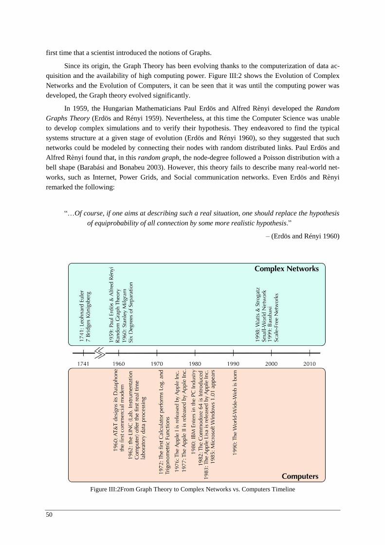
50
first time that a scientist introduced the notions of Graphs.
Since its origin, the Graph Theory has been evolving thanks to the computerization of data ac-quisition and the availability of high computing power. Figure III :2 shows the Evolution of Complex Networks and the Evolution of Computers, it can be seen that it was until the computing power was developed, the Graph theory evolved significantly.
In 1959, the Hungarian Mathematicians Paul Erdös and Alfred Rènyi developed the Random
Graphs Theory (Erdös and Rényi 1959). Nevertheless, at this time the Computer Science was unable to develop complex simulations and to verify their hypothesis. They endeavored to find the typical systems structure at a given stage of evolution (Erdös and Rényi 1960), so they suggested that such networks could be modeled by connecting their nodes with random distributed links. Paul Erdös and Alfred Rènyi found that, in this random graph, the node-degree followed a Poisson distribution with a bell shape (Barabási and Bonabeu 2003). However, this theory fails to describe many real-world net-works, such as Internet, Power Grids, and Social communication networks. Even Erdös and Rènyi remarked the following:
“…Of course, if one aims at describing such a real situation, one should replace the hypothesis
of equiprobability of all connection by some more realistic hypothesis.”
– (Erdös and Rényi 1960)
Figure III :2From Graph Theory to Complex Networks vs. Computers Timeline
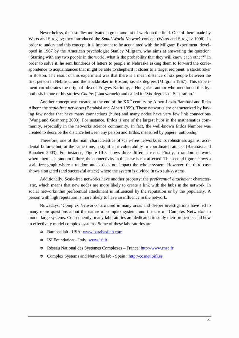
51
Nevertheless, their studies motivated a great amount of work on the field. One of them made by Watts and Strogatz; they introduced the Small-World Network concept (Watts and Strogatz 1998). In order to understand this concept, it is important to be acquainted with the Milgram Experiment, devel-oped in 1967 by the American psychologist Stanley Milgram, who aims at answering the question: “Starting with any two people in the world, what is the probability that they will know each other?” In order to solve it, he sent hundreds of letters to people in Nebraska asking them to forward the corre-spondence to acquaintances that might be able to shepherd it closer to a target recipient: a stockbroker in Boston. The result of this experiment was that there is a mean distance of six people between the first person in Nebraska and the stockbroker in Boston, i.e. six degrees (Milgram 1967). This experi-ment corroborates the original idea of Frigyes Karinthy, a Hungarian author who mentioned this hy-pothesis in one of his stories: Chains (Làncszemek) and called it: ‘Six-degrees of Separation.’
Another concept was created at the end of the XXth century by Albert-Lazlo Barabási and Reka Albert: the scale-free networks (Barabási and Albert 1999). These networks are characterized by hav-ing few nodes that have many connections (hubs) and many nodes have very few link connections (Wang and Guanrong 2003). For instance, Erdös is one of the largest hubs in the mathematics com-munity, especially in the networks science community. In fact, the well-known Erdös Number was created to describe the distance between any person and Erdös, measured by papers’ authorship.
Therefore, one of the main characteristics of scale-free networks is its robustness against acci-dental failures but, at the same time, a significant vulnerability to coordinated attacks (Barabási and Bonabeu 2003). For instance, Figure III :3 shows three different cases. Firstly, a random network where there is a random failure, the connectivity in this case is not affected. The second figure shows a scale-free graph where a random attack does not impact the whole system. However, the third case shows a targeted (and successful attack) where the system is divided in two sub-systems.
Additionally, Scale-free networks have another property: the preferential attachment character-istic, which means that new nodes are more likely to create a link with the hubs in the network. In social networks this preferential attachment is influenced by the reputation or by the popularity. A person with high reputation is more likely to have an influence in the network.
Nowadays, ‘Complex Networks’ are used in many areas and deeper investigations have led to many more questions about the nature of complex systems and the use of ‘Complex Networks’ to model large systems. Consequently, many laboratories are dedicated to study their properties and how to effectively model complex systems. Some of these laboratories are:
Barabasilab - USA: www.barabasilab.com
ISI Foundation – Italy: www.isi.it
Réseau National des Systèmes Complexes – France: http://www.rnsc.fr
Complex Systems and Networks lab - Spain : http://cosnet.bifi.es
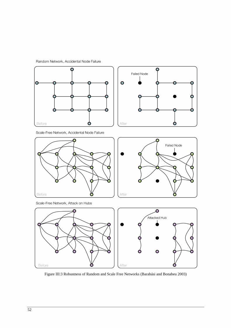
52
Figure III :3 Robustness of Random and Scale Free Networks (Barabási and Bonabeu 2003)
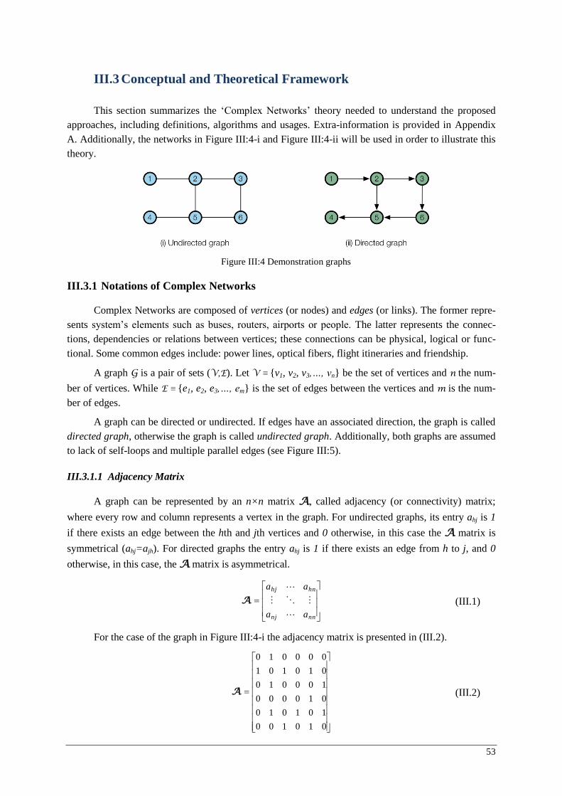
53
III.3 Conceptual and Theoretical Framework
This section summarizes the ‘Complex Networks’ theory needed to understand the proposed approaches, including definitions, algorithms and usages. Extra-information is provided in Appendix A. Additionally, the networks in Figure III :4-i and Figure III :4-ii will be used in order to illustrate this theory.
III.3.1 Notations of Complex Networks
Complex Networks are composed of vertices (or nodes) and edges (or links). The former repre-sents system’s elements such as buses, routers, airports or people. The latter represents the connec-tions, dependencies or relations between vertices; these connections can be physical, logical or func-tional. Some common edges include: power lines, optical fibers, flight itineraries and friendship.
A graph G is a pair of sets (V,E). Let V ≡ {v1, v2, v3,…, vn} be the set of vertices and n the num-
ber of vertices. While E ≡ {e1, e2, e3,…, em} is the set of edges between the vertices and m is the num-ber of edges.
A graph can be directed or undirected. If edges have an associated direction, the graph is called directed graph, otherwise the graph is called undirected graph. Additionally, both graphs are assumed to lack of self-loops and multiple parallel edges (see Figure III :5).
III.3.1.1 Adjacency Matrix
A graph can be represented by an n×n matrix A, called adjacency (or connectivity) matrix;
where every row and column represents a vertex in the graph. For undirected graphs, its entry ahj is 1
if there exists an edge between the hth and jth vertices and 0 otherwise, in this case the A matrix is
symmetrical (ahj=ajh). For directed graphs the entry ahj is 1 if there exists an edge from h to j, and 0
otherwise, in this case, the A matrix is asymmetrical.
nnnj
hnhj
aa
aa
A (III.1)
For the case of the graph in Figure III :4-i the adjacency matrix is presented in (III.2).
010100
101010
010000
100010
010101
000010
A (III.2)
Figure III :4 Demonstration graphs
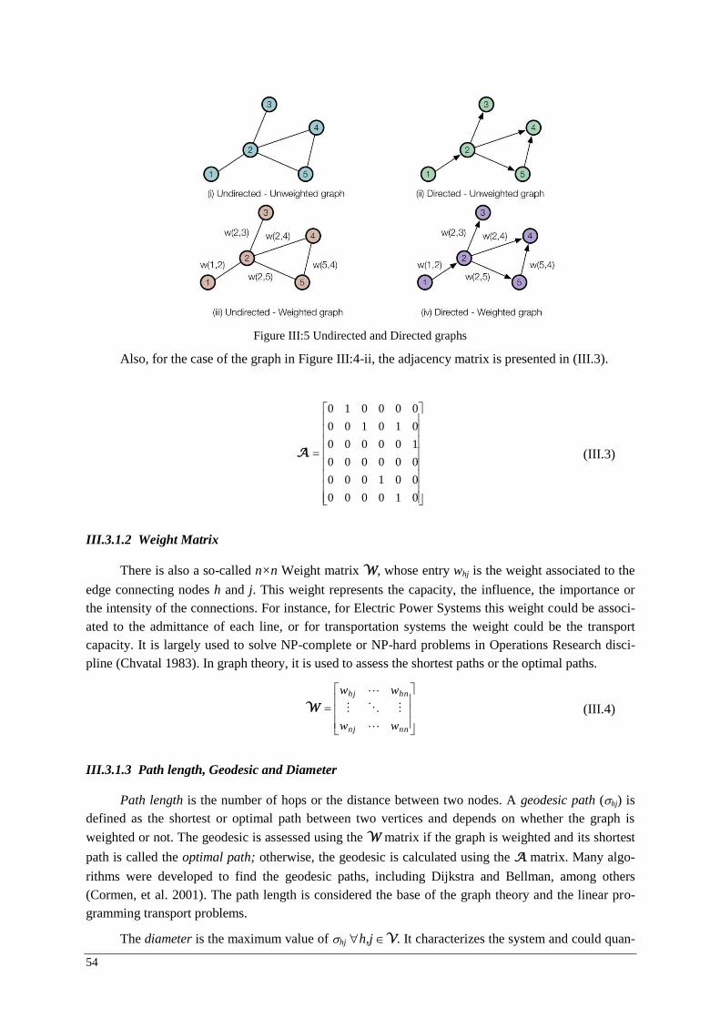
54
Also, for the case of the graph in Figure III :4-ii, the adjacency matrix is presented in (III.3).
010000
001000
000000
100000
010100
000010
A (III.3)
III.3.1.2 Weight Matrix
There is also a so-called n×n Weight matrix W, whose entry whj is the weight associated to the
edge connecting nodes h and j. This weight represents the capacity, the influence, the importance or the intensity of the connections. For instance, for Electric Power Systems this weight could be associ-ated to the admittance of each line, or for transportation systems the weight could be the transport capacity. It is largely used to solve NP-complete or NP-hard problems in Operations Research disci-pline (Chvatal 1983). In graph theory, it is used to assess the shortest paths or the optimal paths.
nnnj
hnhj
ww
ww
W (III.4)
III.3.1.3 Path length, Geodesic and Diameter
Path length is the number of hops or the distance between two nodes. A geodesic path (hj) is defined as the shortest or optimal path between two vertices and depends on whether the graph is
weighted or not. The geodesic is assessed using the W matrix if the graph is weighted and its shortest
path is called the optimal path; otherwise, the geodesic is calculated using the A matrix. Many algo-
rithms were developed to find the geodesic paths, including Dijkstra and Bellman, among others (Cormen, et al. 2001). The path length is considered the base of the graph theory and the linear pro-gramming transport problems.
The diameter is the maximum value of hj h,j V. It characterizes the system and could quan-
Figure III :5 Undirected and Directed graphs
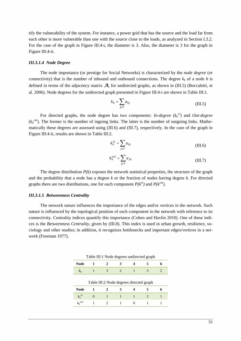
55
tify the vulnerability of the system. For instance, a power grid that has the source and the load far from each other is more vulnerable than one with the source close to the loads, as analyzed in Section I.3.2. For the case of the graph in Figure III :4-i, the diameter is 3. Also, the diameter is 3 for the graph in Figure III :4-ii.
III.3.1.4 Node Degree
The node importance (or prestige for Social Networks) is characterized by the node degree (or connectivity) that is the number of inbound and outbound connections. The degree kh of a node h is
defined in terms of the adjacency matrix A, for undirected graphs, as shown in (III.5) (Boccaletti, et
al. 2006). Node degrees for the undirected graph presented in Figure III :4-i are shown in Table III :1.
Vj
hjh ak (III.5)
For directed graphs, the node degree has two components: In-degree (khin) and Out-degree
(khout). The former is the number of ingoing links. The latter is the number of outgoing links. Mathe-
matically these degrees are assessed using (III.6) and (III.7), respectively. In the case of the graph in Figure III :4-ii, results are shown in Table III :2.
Vj
hjinh ak (III.6)
Vj
jhouth ak (III.7)
The degree distribution P(k) exposes the network statistical properties, the structure of the graph and the probability that a node has a degree k or the fraction of nodes having degree k. For directed graphs there are two distributions, one for each component P(kin) and P(kout).
III.3.1.5 Betweenness Centrality
The network nature influences the importance of the edges and/or vertices in the network. Such nature is influenced by the topological position of each component in the network with reference to its connectivity. Centrality indices quantify this importance (Cohen and Havlin 2010). One of these indi-ces is the Betweenness Centrality, given by (III.8). This index is used in urban growth, resilience, so-ciology and other studies; in addition, it recognizes bottlenecks and important edges/vertices in a net-work (Freeman 1977).
Table III :1 Node degrees undirected graph
Node 1 2 3 4 5 6
kh 1 3 2 1 3 2
Table III :2 Node degrees directed graph
Node 1 2 3 4 5 6
khin 0 1 1 1 2 1
khout 1 2 1 0 1 1
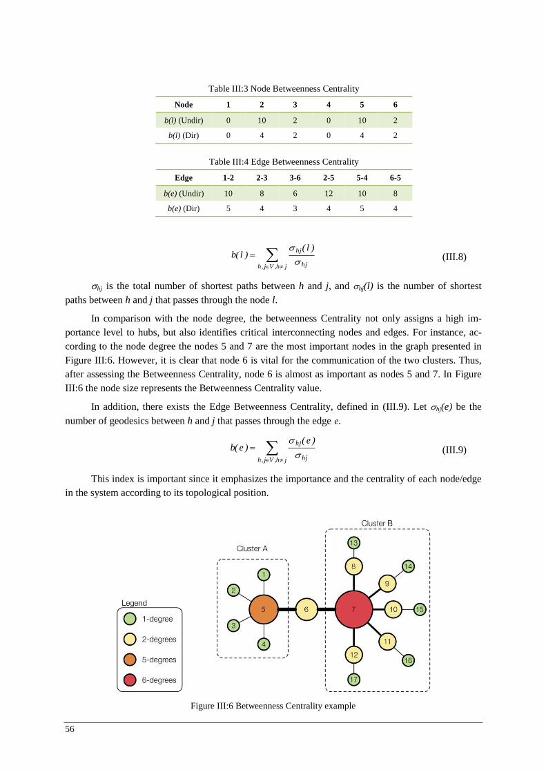
56
jh,Vj,h hj
hj )l()l(b
(III.8)
hj is the total number of shortest paths between h and j, and hj(l) is the number of shortest paths between h and j that passes through the node l.
In comparison with the node degree, the betweenness Centrality not only assigns a high im-portance level to hubs, but also identifies critical interconnecting nodes and edges. For instance, ac-cording to the node degree the nodes 5 and 7 are the most important nodes in the graph presented in Figure III :6. However, it is clear that node 6 is vital for the communication of the two clusters. Thus, after assessing the Betweenness Centrality, node 6 is almost as important as nodes 5 and 7. In Figure III:6 the node size represents the Betweenness Centrality value.
In addition, there exists the Edge Betweenness Centrality, defined in (III.9). Let hj(e) be the
number of geodesics between h and j that passes through the edge e.
jh,Vj,h hj
hj )e()e(b
(III.9)
This index is important since it emphasizes the importance and the centrality of each node/edge in the system according to its topological position.
Table III :3 Node Betweenness Centrality
Node 1 2 3 4 5 6
b(l) (Undir) 0 10 2 0 10 2
b(l) (Dir) 0 4 2 0 4 2
Table III :4 Edge Betweenness Centrality
Edge 1-2 2-3 3-6 2-5 5-4 6-5
b(e) (Undir) 10 8 6 12 10 8
b(e) (Dir) 5 4 3 4 5 4
Figure III :6 Betweenness Centrality example
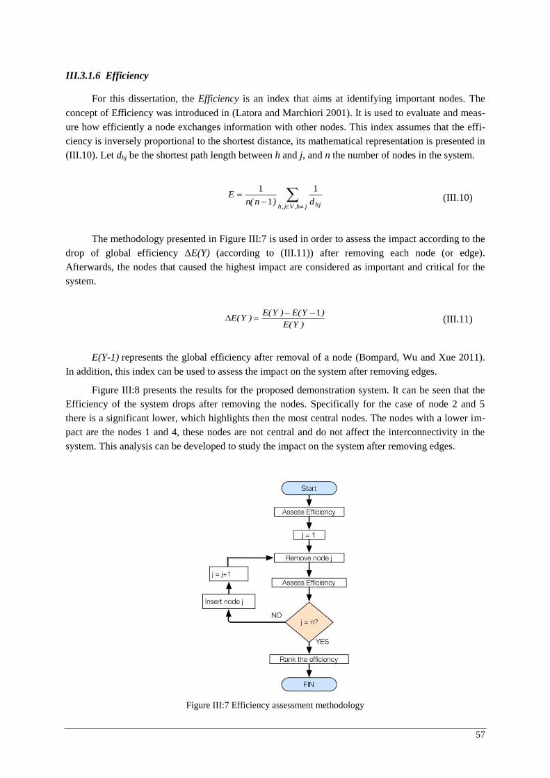
57
III.3.1.6 Efficiency
For this dissertation, the Efficiency is an index that aims at identifying important nodes. The
concept of Efficiency was introduced in (Latora and Marchiori 2001). It is used to evaluate and meas-ure how efficiently a node exchanges information with other nodes. This index assumes that the effi-ciency is inversely proportional to the shortest distance, its mathematical representation is presented in (III.10). Let dhj be the shortest path length between h and j, and n the number of nodes in the system.
jh,Vj,h hjd)n(n
E1
1
1 (III.10)
The methodology presented in Figure III :7 is used in order to assess the impact according to the drop of global efficiency ΔE(Y) (according to (III.11)) after removing each node (or edge). Afterwards, the nodes that caused the highest impact are considered as important and critical for the system.
)Y(E
)Y(E)Y(E)Y(E
1 (III.11)
E(Y-1) represents the global efficiency after removal of a node (Bompard, Wu and Xue 2011). In addition, this index can be used to assess the impact on the system after removing edges.
Figure III :8 presents the results for the proposed demonstration system. It can be seen that the Efficiency of the system drops after removing the nodes. Specifically for the case of node 2 and 5 there is a significant lower, which highlights then the most central nodes. The nodes with a lower im-pact are the nodes 1 and 4, these nodes are not central and do not affect the interconnectivity in the system. This analysis can be developed to study the impact on the system after removing edges.
Figure III :7 Efficiency assessment methodology
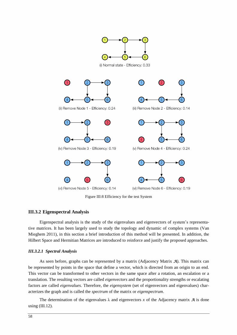
58
III.3.2 Eigenspectral Analysis
Eigenspectral analysis is the study of the eigenvalues and eigenvectors of system’s representa-tive matrices. It has been largely used to study the topology and dynamic of complex systems (Van Mieghem 2011), in this section a brief introduction of this method will be presented. In addition, the Hilbert Space and Hermitian Matrices are introduced to reinforce and justify the proposed approaches.
III.3.2.1 Spectral Analysis
As seen before, graphs can be represented by a matrix (Adjacency Matrix A). This matrix can be represented by points in the space that define a vector, which is directed from an origin to an end. This vector can be transformed to other vectors in the same space after a rotation, an escalation or a translation. The resulting vectors are called eigenvectors and the proportionality strengths or escalating factors are called eigenvalues. Therefore, the eigensystem (set of eigenvectors and eigenvalues) char-acterizes the graph and is called the spectrum of the matrix or eigenspectrum.
The determination of the eigenvalues λ and eigenvectors x of the Adjacency matrix A is done using (III.12).
Figure III :8 Efficiency for the test System
59
xx A (III.12)
Therefore,
0 x)I(xx AA (III.13)
x=0 is a trivial solution to the eigenvalue equation. Thus, to find a non-zero solution for the ho-mogeneous linear system, the matrix A-λI has to be singular16 (III.14).
0det )I( A (III.14)
The matrix spectrum theory has been largely studied in many sciences. Particularly in graph theory, it has been used to develop the partitioning theory or spectral bisection. (Fiedler 1793) found
that the second smallest eigenvalue of the graph’s Laplacian matrix L is a measure of the graph’s con-
nectivity. The Laplacian matrix is defined in (III.15). Let D be a diagonal matrix of degrees. (Rozel, Caire, et al. 2009) applied this theory to study the potential cuts of large interconnected networks.
ADL (III.15)
In addition, the spectrum of the matrix can provide topological information about the system.
III.3.2.2 Hilbert Space
Hilbert Space is defined as a complete, normed and inner product vector space (Hoser 2005).
The following properties have to be followed in a vector space V; where x and y are vectors. These properties will be used to justify the use of Hermitian Matrices in next section.
VV y,xyx (III.16)
V z,y,x)zy(xz)yx( (III.17)
V y,xxyyx (III.18)
V xxx 00 (III.19)
V xxx11 (III.20)
V x)x(x)( 01 (III.21)
V x,aVax C (III.22)
V xb,a)bx(ax)ab( C, (III.23)
V y,x,aayax)yx(a C (III.24)
V xb,abxaxx)ba( C, (III.25)
The inner product is defined in (III.26).
xxx (III.26)
And the following equations have to be hold in a Hilbert Space:
0 ifonly and if0with0 xxxxx (III.27)
16 A Matrix is singular if its determinant is zero.

60
C ayxayax (III.28)
C ayxaayx (III.29)
III.3.2.3 Hermitian Matrices
A matrix is defined as a Hermitian Matrix if and only if accomplishes the equation (III.30)17.
*HH (III.30)
Where,
lkkl hh (III.31)
The main interest on Hermitian Matrices in the Hilbert Space is that their Eigenvalues, assessed
with (III.32), are all reals ( kk ). This property enables the important or more prestigious nodes
to be classified and ranked.
λxx H (III.32)
An example of a Hermitian matrix is shown in (III.33).
7518
51594
9632
84321
iii
ii
iii
ii
H (III.33)
The eigenvalues from this matrix are presented in (III.34), it can be seen that they are real val-ues and the eigenvectors, in (III.35), are complex numbers.
6171687910172266810 ....λ (III.34)
500650380430
580150350150420210510130
100570130350110580180380
220930540090530010600030
....
i..i..i..i..
i..i..i..i..
i..i..i..i..
x (III.35)
17 H* is the conjugate transpose of H.
Proof of kk (Hoser 2005):
a. λxx H
b. xxλxλxxx H from (III.28)
c. xxλλxxxx H from (III.29)
d. Since *HH , then xxxx HH
e. xxλxxλ
f.
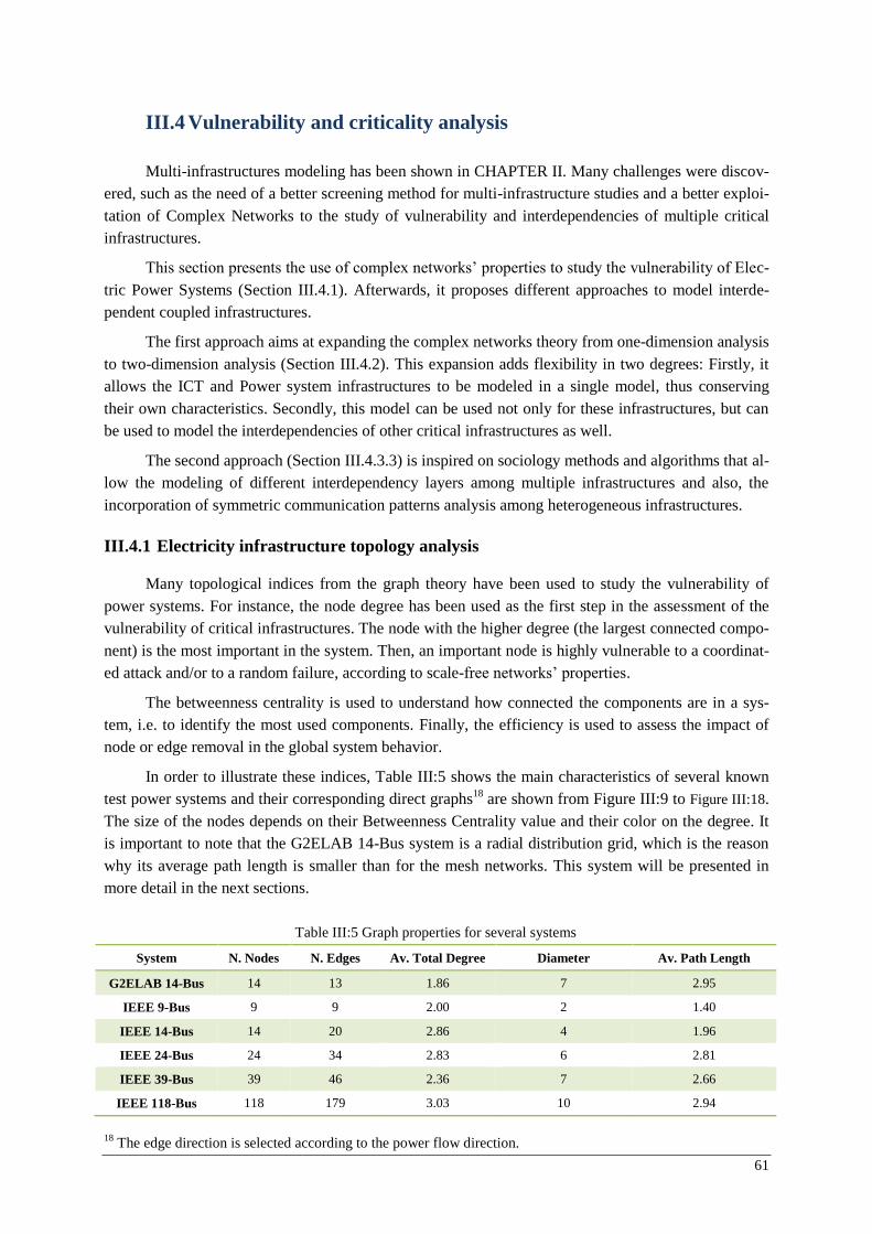
61
III.4 Vulnerability and criticality analysis
Multi-infrastructures modeling has been shown in CHAPTER II. Many challenges were discov-ered, such as the need of a better screening method for multi-infrastructure studies and a better exploi-tation of Complex Networks to the study of vulnerability and interdependencies of multiple critical infrastructures.
This section presents the use of complex networks’ properties to study the vulnerability of Elec-tric Power Systems (Section III.4.1). Afterwards, it proposes different approaches to model interde-pendent coupled infrastructures.
The first approach aims at expanding the complex networks theory from one-dimension analysis to two-dimension analysis (Section III.4.2). This expansion adds flexibility in two degrees: Firstly, it allows the ICT and Power system infrastructures to be modeled in a single model, thus conserving their own characteristics. Secondly, this model can be used not only for these infrastructures, but can be used to model the interdependencies of other critical infrastructures as well.
The second approach (Section III.4.3.3) is inspired on sociology methods and algorithms that al-low the modeling of different interdependency layers among multiple infrastructures and also, the incorporation of symmetric communication patterns analysis among heterogeneous infrastructures.
III.4.1 Electricity infrastructure topology analysis
Many topological indices from the graph theory have been used to study the vulnerability of power systems. For instance, the node degree has been used as the first step in the assessment of the vulnerability of critical infrastructures. The node with the higher degree (the largest connected compo-nent) is the most important in the system. Then, an important node is highly vulnerable to a coordinat-ed attack and/or to a random failure, according to scale-free networks’ properties.
The betweenness centrality is used to understand how connected the components are in a sys-tem, i.e. to identify the most used components. Finally, the efficiency is used to assess the impact of node or edge removal in the global system behavior.
In order to illustrate these indices, Table III :5 shows the main characteristics of several known test power systems and their corresponding direct graphs18 are shown from Figure III :9 to Figure III :18. The size of the nodes depends on their Betweenness Centrality value and their color on the degree. It is important to note that the G2ELAB 14-Bus system is a radial distribution grid, which is the reason why its average path length is smaller than for the mesh networks. This system will be presented in more detail in the next sections.
18 The edge direction is selected according to the power flow direction.
Table III :5 Graph properties for several systems
System N. Nodes N. Edges Av. Total Degree Diameter Av. Path Length
G2ELAB 14-Bus 14 13 1.86 7 2.95
IEEE 9-Bus 9 9 2.00 2 1.40
IEEE 14-Bus 14 20 2.86 4 1.96
IEEE 24-Bus 24 34 2.83 6 2.81
IEEE 39-Bus 39 46 2.36 7 2.66
IEEE 118-Bus 118 179 3.03 10 2.94
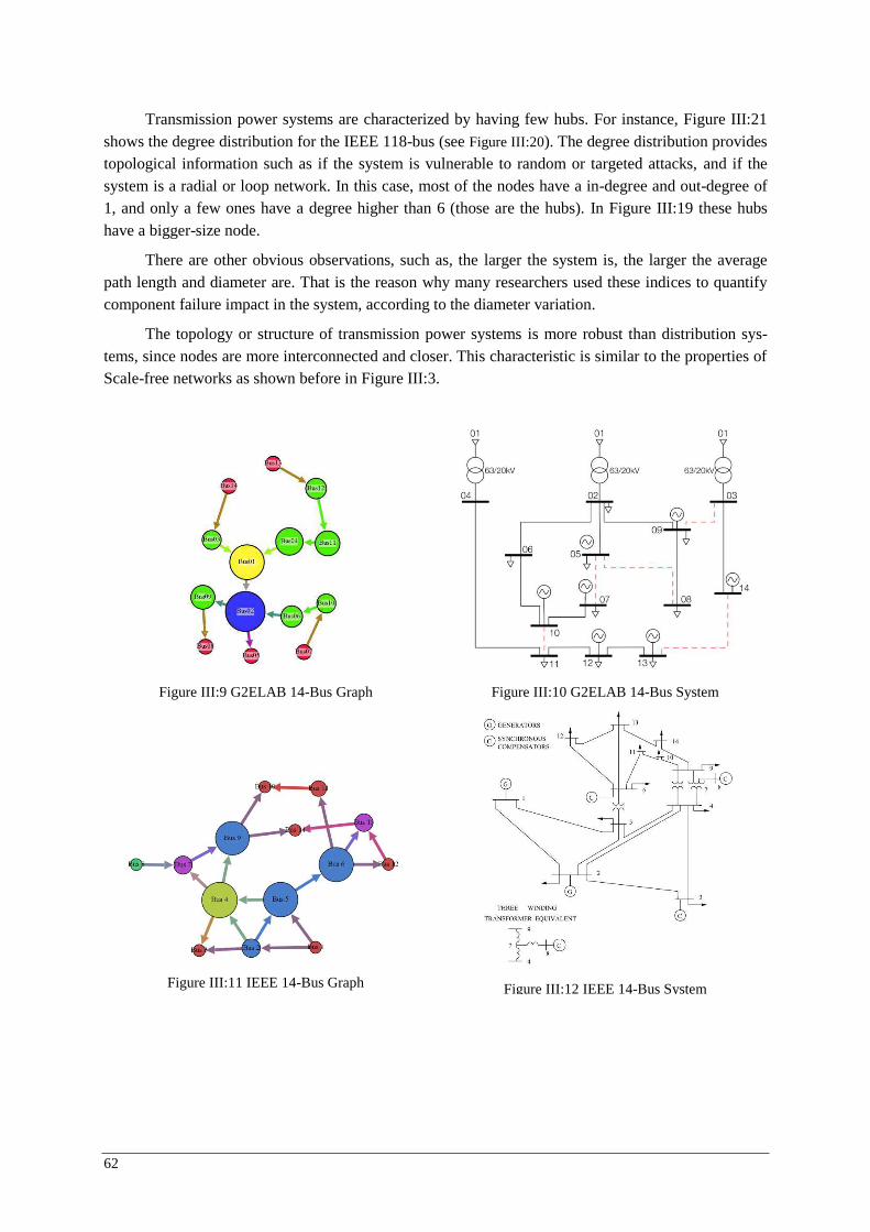
62
Transmission power systems are characterized by having few hubs. For instance, Figure III :21 shows the degree distribution for the IEEE 118-bus (see Figure III :20). The degree distribution provides topological information such as if the system is vulnerable to random or targeted attacks, and if the system is a radial or loop network. In this case, most of the nodes have a in-degree and out-degree of 1, and only a few ones have a degree higher than 6 (those are the hubs). In Figure III :19 these hubs have a bigger-size node.
There are other obvious observations, such as, the larger the system is, the larger the average path length and diameter are. That is the reason why many researchers used these indices to quantify component failure impact in the system, according to the diameter variation.
The topology or structure of transmission power systems is more robust than distribution sys-tems, since nodes are more interconnected and closer. This characteristic is similar to the properties of Scale-free networks as shown before in Figure III :3.
Figure III :9 G2ELAB 14-Bus Graph
Figure III :10 G2ELAB 14-Bus System
Figure III :11 IEEE 14-Bus Graph
Figure III :12 IEEE 14-Bus System
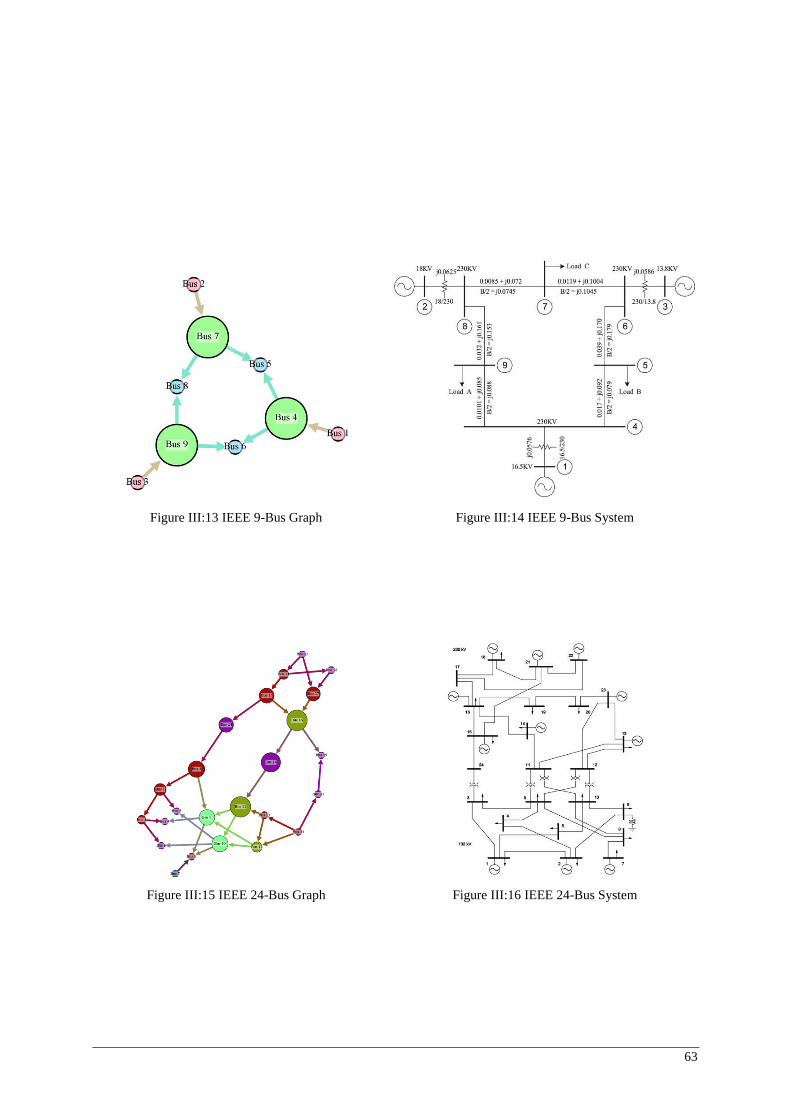
63
Figure III :13 IEEE 9-Bus Graph
Figure III :14 IEEE 9-Bus System
Figure III :15 IEEE 24-Bus Graph
Figure III :16 IEEE 24-Bus System
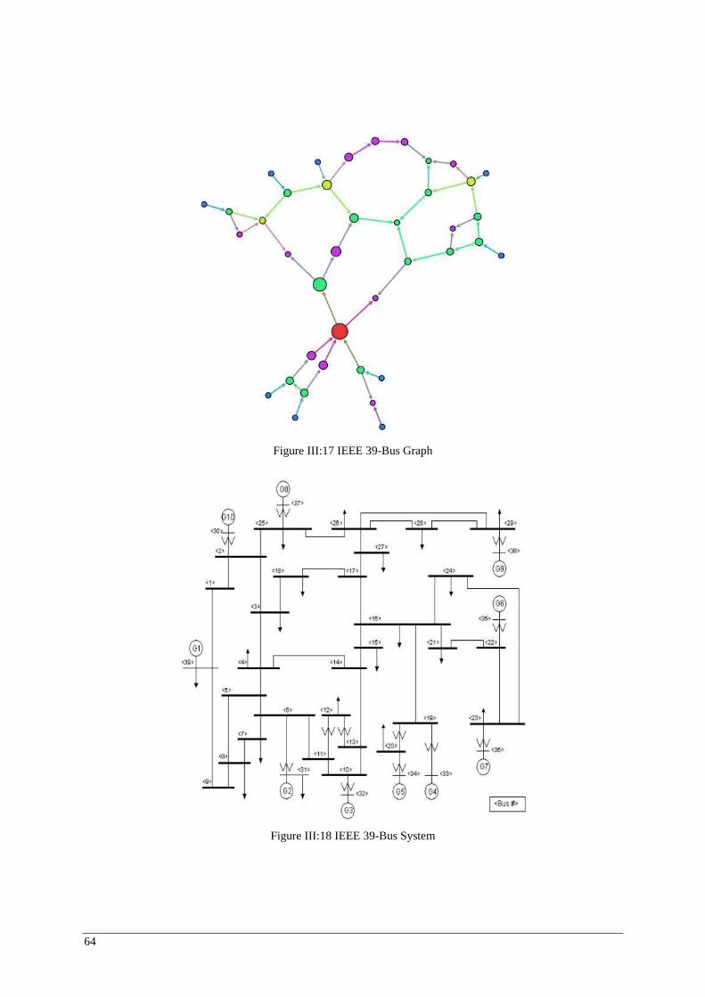
64
Figure III :17 IEEE 39-Bus Graph
Figure III :18 IEEE 39-Bus System
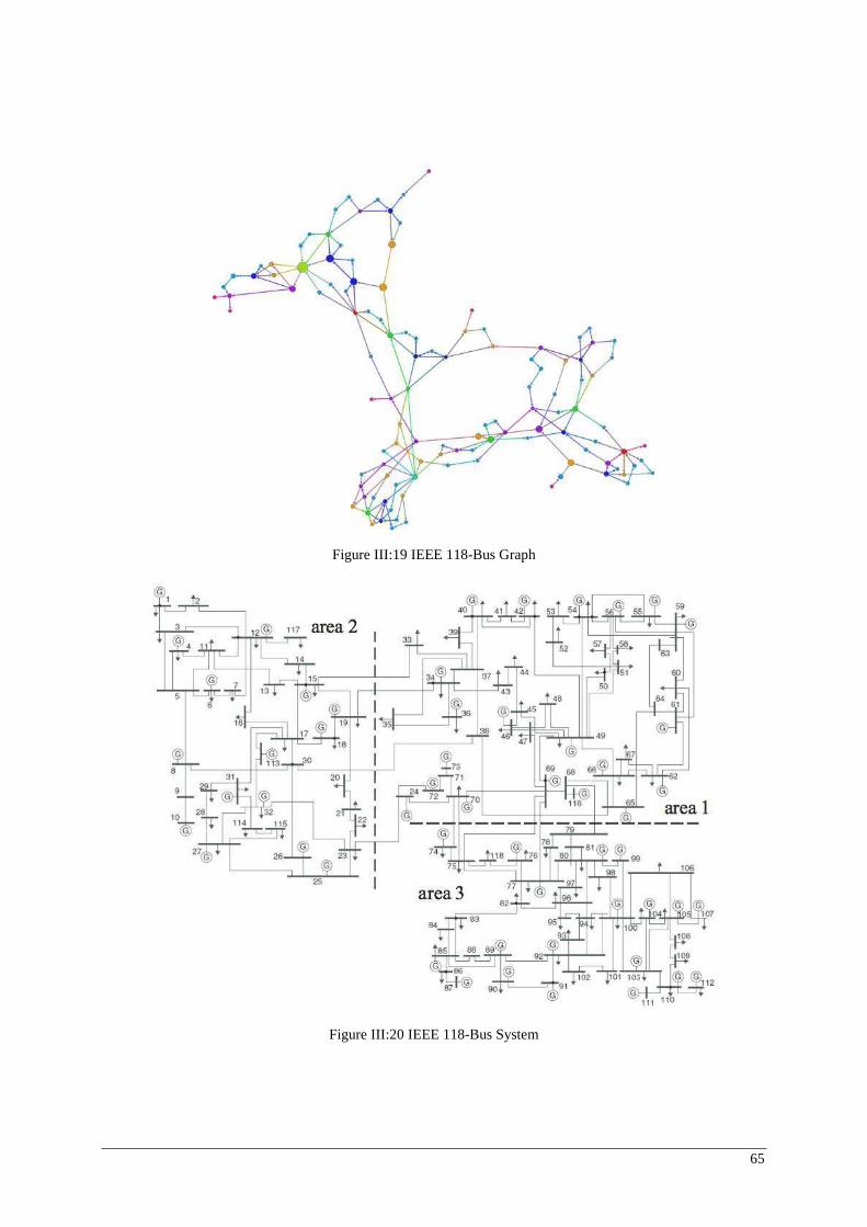
65
Figure III :19 IEEE 118-Bus Graph
Figure III :20 IEEE 118-Bus System
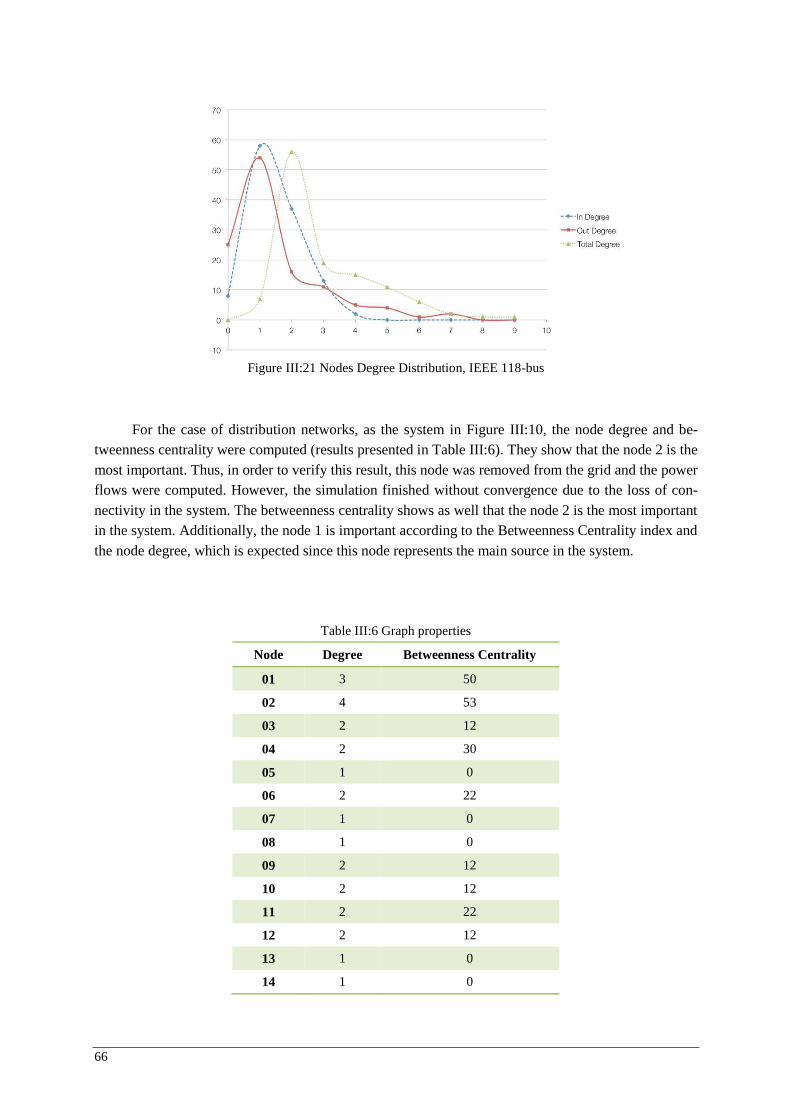
66
For the case of distribution networks, as the system in Figure III :10, the node degree and be-tweenness centrality were computed (results presented in Table III :6). They show that the node 2 is the most important. Thus, in order to verify this result, this node was removed from the grid and the power flows were computed. However, the simulation finished without convergence due to the loss of con-nectivity in the system. The betweenness centrality shows as well that the node 2 is the most important in the system. Additionally, the node 1 is important according to the Betweenness Centrality index and the node degree, which is expected since this node represents the main source in the system.
Figure III :21 Nodes Degree Distribution, IEEE 118-bus
Table III :6 Graph properties
Node Degree Betweenness Centrality
01 3 50
02 4 53
03 2 12
04 2 30
05 1 0
06 2 22
07 1 0
08 1 0
09 2 12
10 2 12
11 2 22
12 2 12
13 1 0
14 1 0
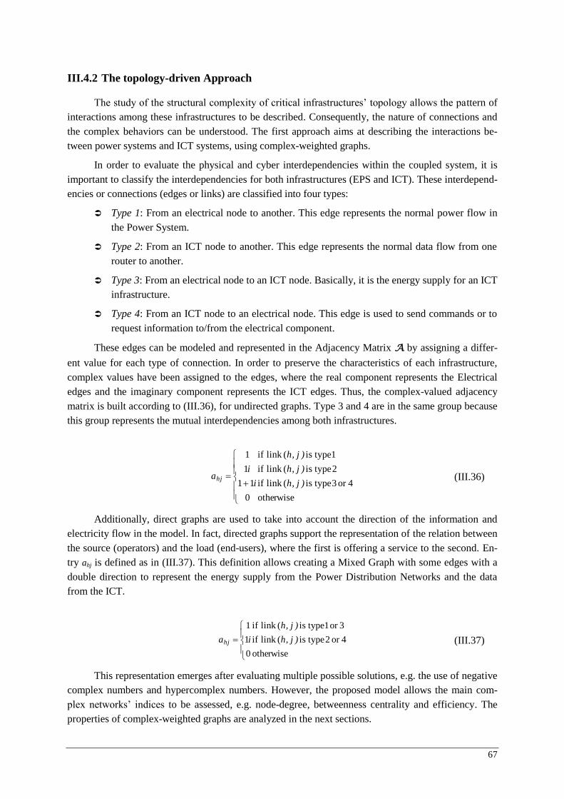
67
III.4.2 The topology-driven Approach
The study of the structural complexity of critical infrastructures’ topology allows the pattern of interactions among these infrastructures to be described. Consequently, the nature of connections and the complex behaviors can be understood. The first approach aims at describing the interactions be-tween power systems and ICT systems, using complex-weighted graphs.
In order to evaluate the physical and cyber interdependencies within the coupled system, it is important to classify the interdependencies for both infrastructures (EPS and ICT). These interdepend-encies or connections (edges or links) are classified into four types:
Type 1: From an electrical node to another. This edge represents the normal power flow in the Power System.
Type 2: From an ICT node to another. This edge represents the normal data flow from one router to another.
Type 3: From an electrical node to an ICT node. Basically, it is the energy supply for an ICT infrastructure.
Type 4: From an ICT node to an electrical node. This edge is used to send commands or to request information to/from the electrical component.
These edges can be modeled and represented in the Adjacency Matrix A by assigning a differ-
ent value for each type of connection. In order to preserve the characteristics of each infrastructure, complex values have been assigned to the edges, where the real component represents the Electrical edges and the imaginary component represents the ICT edges. Thus, the complex-valued adjacency matrix is built according to (III.36), for undirected graphs. Type 3 and 4 are in the same group because this group represents the mutual interdependencies among both infrastructures.
otherwise
4or 3 typeis (link if
2 typeis (link if
1 typeis (link if
0
11
1
1
)j,h
)j,h
)j,h
i
iahj (III.36)
Additionally, direct graphs are used to take into account the direction of the information and electricity flow in the model. In fact, directed graphs support the representation of the relation between the source (operators) and the load (end-users), where the first is offering a service to the second. En-try ahj is defined as in (III.37). This definition allows creating a Mixed Graph with some edges with a double direction to represent the energy supply from the Power Distribution Networks and the data from the ICT.
otherwise
4or 2 typeis (link if
3or 1 typeis (link if
0
1
1
)j,h
)j,h
iahj (III.37)
This representation emerges after evaluating multiple possible solutions, e.g. the use of negative complex numbers and hypercomplex numbers. However, the proposed model allows the main com-plex networks’ indices to be assessed, e.g. node-degree, betweenness centrality and efficiency. The properties of complex-weighted graphs are analyzed in the next sections.
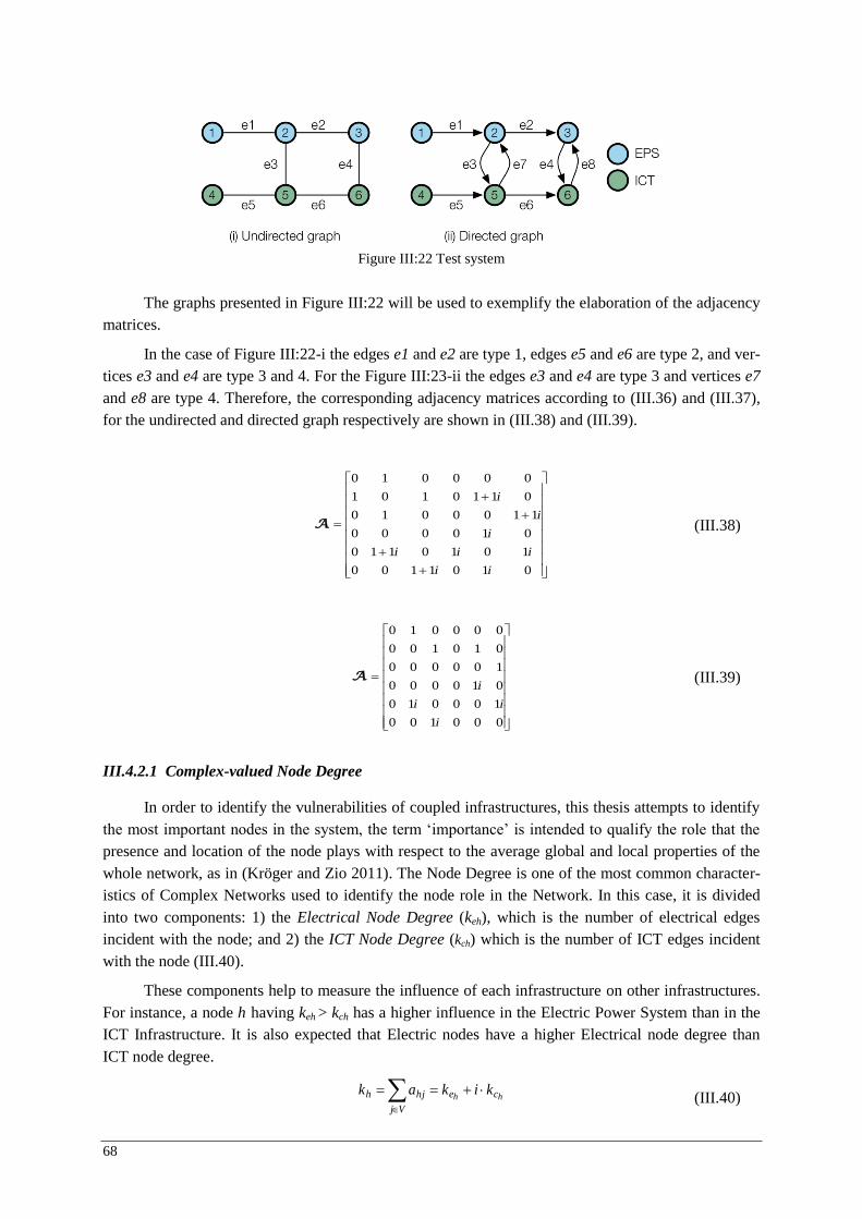
68
The graphs presented in Figure III :22 will be used to exemplify the elaboration of the adjacency matrices.
In the case of Figure III :22-i the edges e1 and e2 are type 1, edges e5 and e6 are type 2, and ver-tices e3 and e4 are type 3 and 4. For the Figure III :23-ii the edges e3 and e4 are type 3 and vertices e7 and e8 are type 4. Therefore, the corresponding adjacency matrices according to (III.36) and (III.37), for the undirected and directed graph respectively are shown in (III.38) and (III.39).
0101100
1010110
010000
1100010
0110101
000010
ii
iii
i
i
i
A
(III.38)
000100
100010
010000
100000
010100
000010
i
ii
iA
(III.39)
III.4.2.1 Complex-valued Node Degree
In order to identify the vulnerabilities of coupled infrastructures, this thesis attempts to identify the most important nodes in the system, the term ‘importance’ is intended to qualify the role that the presence and location of the node plays with respect to the average global and local properties of the whole network, as in (Kröger and Zio 2011). The Node Degree is one of the most common character-istics of Complex Networks used to identify the node role in the Network. In this case, it is divided into two components: 1) the Electrical Node Degree (keh), which is the number of electrical edges incident with the node; and 2) the ICT Node Degree (kch) which is the number of ICT edges incident with the node (III.40).
These components help to measure the influence of each infrastructure on other infrastructures. For instance, a node h having keh > kch has a higher influence in the Electric Power System than in the ICT Infrastructure. It is also expected that Electric nodes have a higher Electrical node degree than ICT node degree.
hh ce
Vj
hjh kikak (III.40)
Figure III :22 Test system
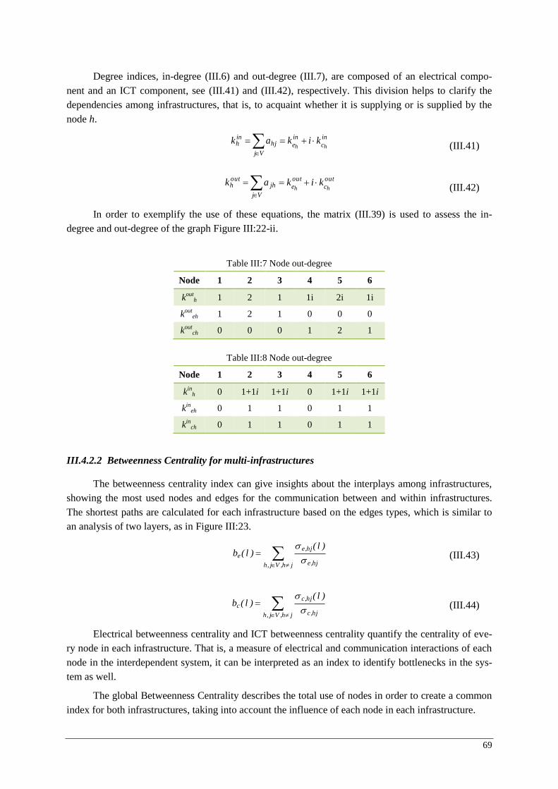
69
Degree indices, in-degree (III.6) and out-degree (III.7), are composed of an electrical compo-nent and an ICT component, see (III.41) and (III.42), respectively. This division helps to clarify the dependencies among infrastructures, that is, to acquaint whether it is supplying or is supplied by the node h.
inc
ine
Vj
hjinh hh
kikak (III.41)
outc
oute
Vj
jhouth hh
kikak (III.42)
In order to exemplify the use of these equations, the matrix (III.39) is used to assess the in-degree and out-degree of the graph Figure III :22-ii.
III.4.2.2 Betweenness Centrality for multi-infrastructures
The betweenness centrality index can give insights about the interplays among infrastructures, showing the most used nodes and edges for the communication between and within infrastructures. The shortest paths are calculated for each infrastructure based on the edges types, which is similar to an analysis of two layers, as in Figure III :23.
jh,Vj,h hj,e
hj,ee
)l()l(b
(III.43)
jh,Vj,h hj,c
hj,cc
)l()l(b
(III.44)
Electrical betweenness centrality and ICT betweenness centrality quantify the centrality of eve-ry node in each infrastructure. That is, a measure of electrical and communication interactions of each node in the interdependent system, it can be interpreted as an index to identify bottlenecks in the sys-tem as well.
The global Betweenness Centrality describes the total use of nodes in order to create a common index for both infrastructures, taking into account the influence of each node in each infrastructure.
Table III :7 Node out-degree
Node 1 2 3 4 5 6
kouth 1 2 1 1i 2i 1i
kouteh 1 2 1 0 0 0
koutch 0 0 0 1 2 1
Table III :8 Node out-degree
Node 1 2 3 4 5 6
kinh 0 1+1i 1+1i 0 1+1i 1+1i
kineh 0 1 1 0 1 1
kinch 0 1 1 0 1 1
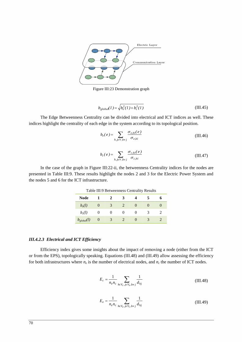
70
)l(b)l(b)l(b ceglobal22 (III.45)
The Edge Betweenness Centrality can be divided into electrical and ICT indices as well. These indices highlight the centrality of each edge in the system according to its topological position.
jh,Vj,h hl,e
hl,ee
)e()e(b
(III.46)
jh,Vj,h hl,c
hl,cc
)e()e(b
(III.47)
In the case of the graph in Figure III :22-ii, the betweenness Centrality indices for the nodes are presented in Table III :9. These results highlight the nodes 2 and 3 for the Electric Power System and the nodes 5 and 6 for the ICT infrastructure.
III.4.2.3 Electrical and ICT Efficiency
Efficiency index gives some insights about the impact of removing a node (either from the ICT or from the EPS), topologically speaking. Equations (III.48) and (III.49) allow assessing the efficiency for both infrastructures where ne is the number of electrical nodes, and nc the number of ICT nodes.
jh,Vj,Vh hjcec
ecdnn
E11
(III.48)
jh,Vj,Vh hjcee
cednn
E11
(III.49)
Table III :9 Betweenness Centrality Results
Node 1 2 3 4 5 6
be(l) 0 3 2 0 0 0
bc(l) 0 0 0 0 3 2
bglobal(l) 0 3 2 0 3 2
Figure III :23 Demonstration graph
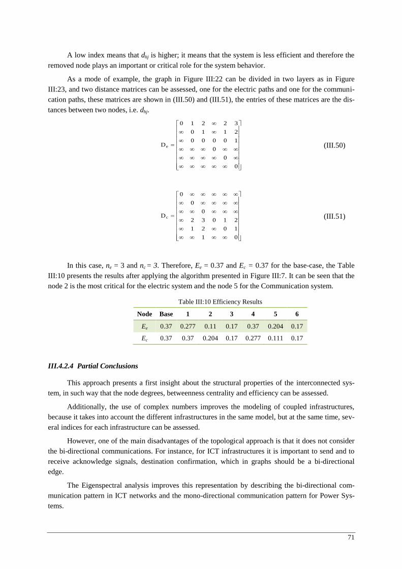
71
A low index means that dhj is higher; it means that the system is less efficient and therefore the removed node plays an important or critical role for the system behavior.
As a mode of example, the graph in Figure III :22 can be divided in two layers as in Figure III:23, and two distance matrices can be assessed, one for the electric paths and one for the communi-cation paths, these matrices are shown in (III.50) and (III.51), the entries of these matrices are the dis-tances between two nodes, i.e. dhj.
0
0
0
10000
2110
32210
De
(III.50)
01
1021
21032
0
0
0
Dc
(III.51)
In this case, ne = 3 and nc = 3. Therefore, Ee = 0.37 and Ec = 0.37 for the base-case, the Table III:10 presents the results after applying the algorithm presented in Figure III :7. It can be seen that the node 2 is the most critical for the electric system and the node 5 for the Communication system.
III.4.2.4 Partial Conclusions
This approach presents a first insight about the structural properties of the interconnected sys-tem, in such way that the node degrees, betweenness centrality and efficiency can be assessed.
Additionally, the use of complex numbers improves the modeling of coupled infrastructures, because it takes into account the different infrastructures in the same model, but at the same time, sev-eral indices for each infrastructure can be assessed.
However, one of the main disadvantages of the topological approach is that it does not consider the bi-directional communications. For instance, for ICT infrastructures it is important to send and to receive acknowledge signals, destination confirmation, which in graphs should be a bi-directional edge.
The Eigenspectral analysis improves this representation by describing the bi-directional com-munication pattern in ICT networks and the mono-directional communication pattern for Power Sys-tems.
Table III :10 Efficiency Results
Node Base 1 2 3 4 5 6
Ee 0.37 0.277 0.11 0.17 0.37 0.204 0.17
Ec 0.37 0.37 0.204 0.17 0.277 0.111 0.17
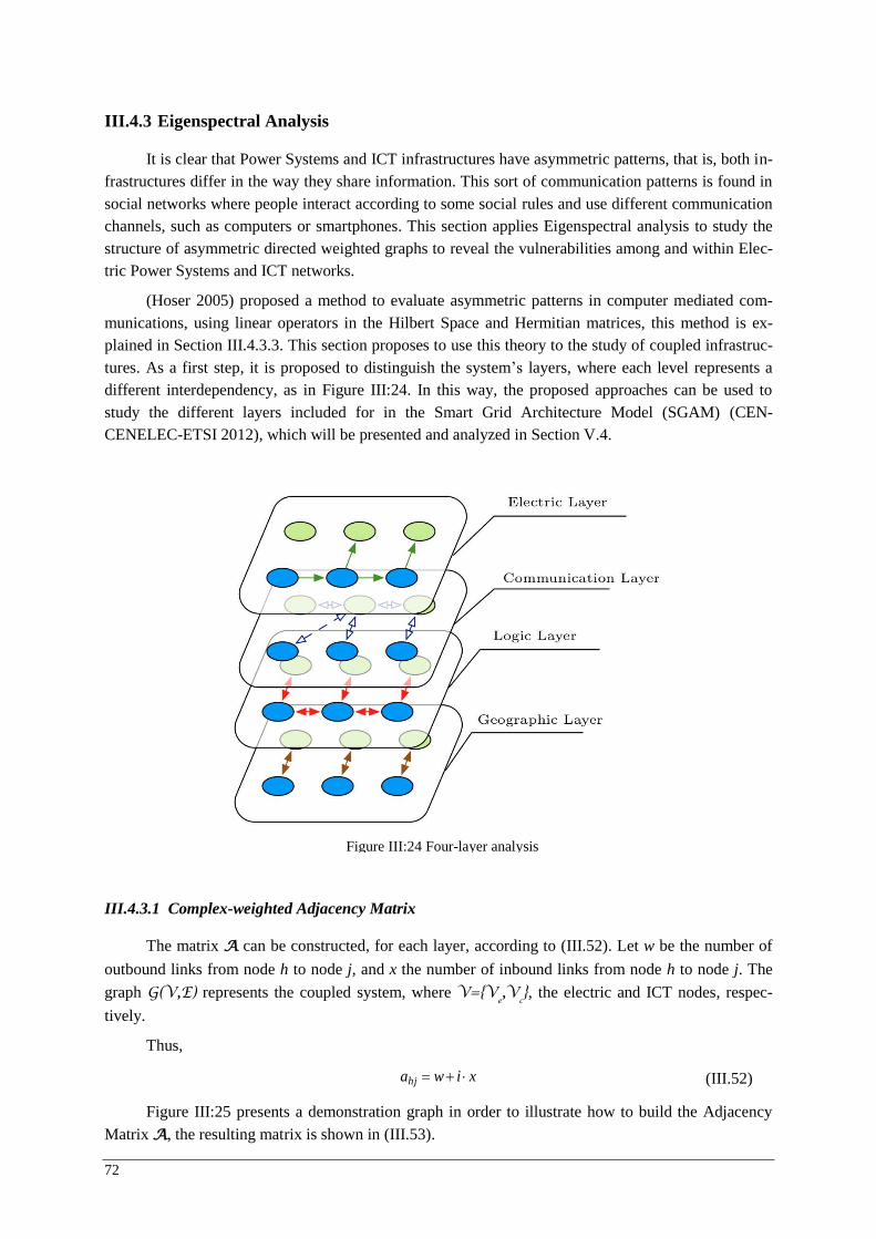
72
III.4.3 Eigenspectral Analysis
It is clear that Power Systems and ICT infrastructures have asymmetric patterns, that is, both in-frastructures differ in the way they share information. This sort of communication patterns is found in social networks where people interact according to some social rules and use different communication channels, such as computers or smartphones. This section applies Eigenspectral analysis to study the structure of asymmetric directed weighted graphs to reveal the vulnerabilities among and within Elec-tric Power Systems and ICT networks.
(Hoser 2005) proposed a method to evaluate asymmetric patterns in computer mediated com-munications, using linear operators in the Hilbert Space and Hermitian matrices, this method is ex-plained in Section III.4.3.3. This section proposes to use this theory to the study of coupled infrastruc-tures. As a first step, it is proposed to distinguish the system’s layers, where each level represents a different interdependency, as in Figure III :24. In this way, the proposed approaches can be used to study the different layers included for in the Smart Grid Architecture Model (SGAM) (CEN-CENELEC-ETSI 2012), which will be presented and analyzed in Section V.4.
III.4.3.1 Complex-weighted Adjacency Matrix
The matrix A can be constructed, for each layer, according to (III.52). Let w be the number of
outbound links from node h to node j, and x the number of inbound links from node h to node j. The
graph G(V,E) represents the coupled system, where V={Ve,V
c}, the electric and ICT nodes, respec-
tively.
Thus,
xiwahj (III.52)
Figure III :25 presents a demonstration graph in order to illustrate how to build the Adjacency Matrix A, the resulting matrix is shown in (III.53).
Figure III :24 Four-layer analysis
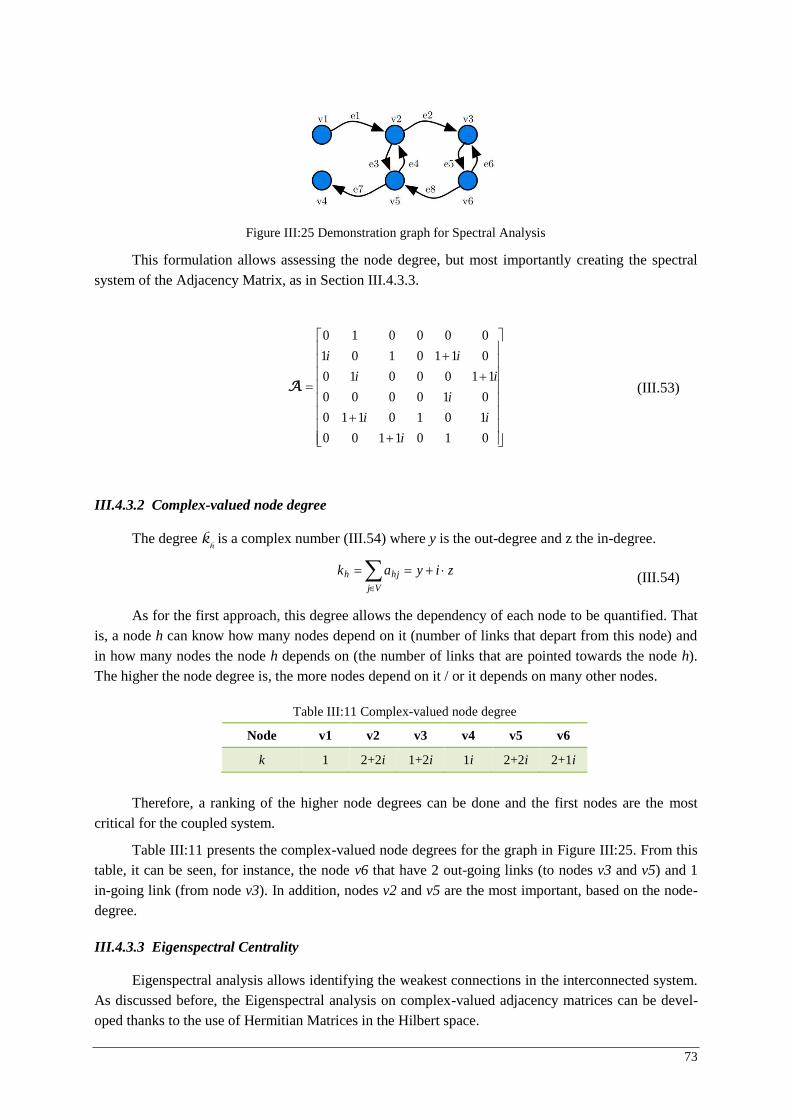
73
This formulation allows assessing the node degree, but most importantly creating the spectral system of the Adjacency Matrix, as in Section III.4.3.3.
0101100
1010110
010000
1100010
0110101
000010
i
ii
i
ii
ii
A (III.53)
III.4.3.2 Complex-valued node degree
The degree kh is a complex number (III.54) where y is the out-degree and z the in-degree.
ziyakVj
hjh (III.54)
As for the first approach, this degree allows the dependency of each node to be quantified. That is, a node h can know how many nodes depend on it (number of links that depart from this node) and in how many nodes the node h depends on (the number of links that are pointed towards the node h). The higher the node degree is, the more nodes depend on it / or it depends on many other nodes.
Therefore, a ranking of the higher node degrees can be done and the first nodes are the most critical for the coupled system.
Table III :11 presents the complex-valued node degrees for the graph in Figure III :25. From this table, it can be seen, for instance, the node v6 that have 2 out-going links (to nodes v3 and v5) and 1 in-going link (from node v3). In addition, nodes v2 and v5 are the most important, based on the node-degree.
III.4.3.3 Eigenspectral Centrality
Eigenspectral analysis allows identifying the weakest connections in the interconnected system. As discussed before, the Eigenspectral analysis on complex-valued adjacency matrices can be devel-oped thanks to the use of Hermitian Matrices in the Hilbert space.
Figure III :25 Demonstration graph for Spectral Analysis
Table III :11 Complex-valued node degree
Node v1 v2 v3 v4 v5 v6
k 1 2+2i 1+2i 1i 2+2i 2+1i
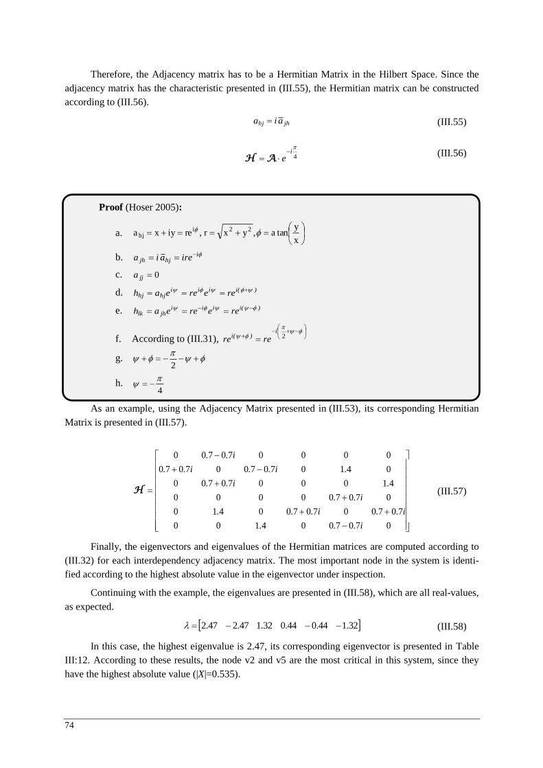
74
Therefore, the Adjacency matrix has to be a Hermitian Matrix in the Hilbert Space. Since the adjacency matrix has the characteristic presented in (III.55), the Hermitian matrix can be constructed according to (III.56).
jhhj aia (III.55)
4
i
e AH (III.56)
As an example, using the Adjacency Matrix presented in (III.53), its corresponding Hermitian Matrix is presented in (III.57).
0707004100
7070070700410
070700000
4100070700
0410707007070
000070700
i...
i..i...
i..
.i..
.i..i..
i..
H (III.57)
Finally, the eigenvectors and eigenvalues of the Hermitian matrices are computed according to (III.32) for each interdependency adjacency matrix. The most important node in the system is identi-fied according to the highest absolute value in the eigenvector under inspection.
Continuing with the example, the eigenvalues are presented in (III.58), which are all real-values, as expected.
32.144.044.032.147.247.2 (III.58)
In this case, the highest eigenvalue is 2.47, its corresponding eigenvector is presented in Table III:12. According to these results, the node v2 and v5 are the most critical in this system, since they have the highest absolute value (|X|=0.535).
Proof (Hoser 2005):
a.
x
ytana,yxr,reiyxa 22i
hj
b. ihjjh ireaia
c. 0jja
d. )(iiiihjhj reereeah
e. )(iiiijhlk reereeah
f. According to (III.31),
2
i)(i rere
g. 2
h. 4
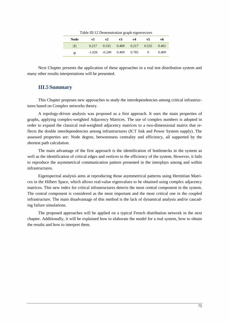
75
Next Chapter presents the application of these approaches in a real test distribution system and many other results interpretations will be presented.
III.5 Summary
This Chapter proposes new approaches to study the interdependencies among critical infrastruc-tures based on Complex networks theory.
A topology-driven analysis was proposed as a first approach. It uses the main properties of graphs, applying complex-weighted Adjacency Matrices. The use of complex numbers is adopted in order to expand the classical real-weighted adjacency matrices to a two-dimensional matrix that re-flects the double interdependencies among infrastructures (ICT link and Power System supply). The assessed properties are: Node degree, betweenness centrality and efficiency, all supported by the shortest path calculation.
The main advantage of the first approach is the identification of bottlenecks in the system as well as the identification of critical edges and vertices to the efficiency of the system. However, it fails to reproduce the asymmetrical communication pattern presented in the interplays among and within infrastructures.
Eigenspectral analysis aims at reproducing those asymmetrical patterns using Hermitian Matri-ces in the Hilbert Space, which allows real-value eigenvalues to be obtained using complex adjacency matrices. This new index for critical infrastructures detects the most central component in the system. The central component is considered as the most important and the most critical one in the coupled infrastructure. The main disadvantage of this method is the lack of dynamical analysis and/or cascad-ing failure simulations.
The proposed approaches will be applied on a typical French distribution network in the next chapter. Additionally, it will be explained how to elaborate the model for a real system, how to obtain the results and how to interpret them.
Table III :12 Demonstration graph eigenvectors
Node v1 v2 v3 v4 v5 v6
|X| 0.217 0.535 0.409 0.217 0.535 0.401
φ -1.026 -0.240 0.409 0.785 0 0.409

77
CHAPTER IV
Vulnerability and Interdependencies: Application
The perplexity of life arises from there being too many interesting
things in it for us to be interested properly in any of them
Gilbert Keith Chesterton
TABLE OF CONTENTS
IV.1 TEST SYSTEM ................................................................................................................. 78
IV.2 TOPOLOGICAL APPROACH RESULTS ............................................................................. 79
IV.2.1 Adjacency Matrix ............................................................................................ 80
IV.2.2 Complex-valued Node Degree ........................................................................ 81
IV.2.3 Betweenness Centrality Analysis .................................................................... 86
IV.2.4 Efficiency ........................................................................................................ 88
IV.2.5 Results Analysis .............................................................................................. 90
IV.3 EIGENSPECTRAL APPROACH RESULTS .......................................................................... 93
IV.3.1 Complex-valued Node Degree ........................................................................ 94
IV.3.2 Prestige Analysis ............................................................................................. 95
IV.4 CONCLUSIONS ................................................................................................................ 98
Abstract
This chapter applies the mathematical approaches proposed in the previous chapter on a typical French
distribution system, including the topology-driven analysis and the Eigenspectral analysis. The results obtained
from these approaches allow the identification of components and connections that have an important topologi-
cal role in the coupled system. In addition, the approaches provide important indices that are used as a quantifi-
cation of weaknesses in the system. Finally, results from both approaches are compared an analyzed.
In the previous chapters we have presented a real problematic that emerge from the interactions and interplays among critical infrastructures, including Power Systems and ICT systems. The state-of-the-art in CHAPTER II reveals the need for new tools to study interdependencies and vulnerabilities among critical infrastructures. In response to these problems, two approaches are proposed in CHAP-TER III, using complex networks theory and several indices and methodologies are proposed. This Chapter focuses on the application of the proposed approaches in order to exemplify their utilization
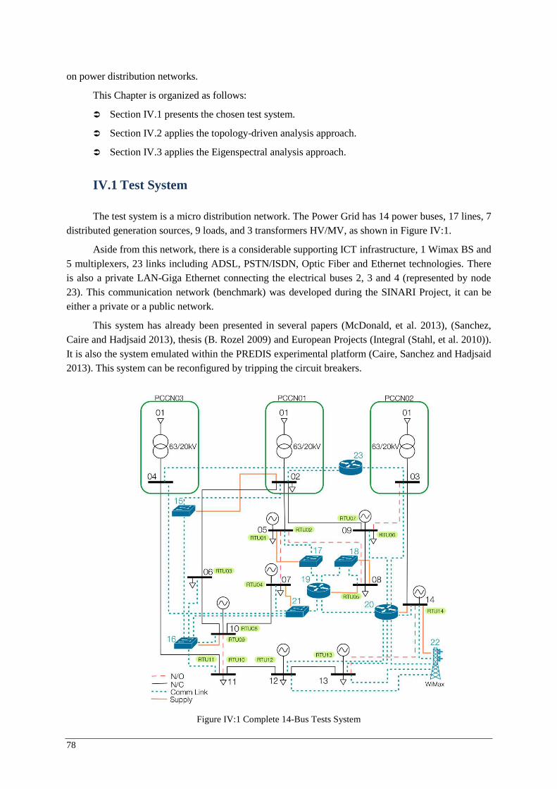
78
on power distribution networks.
This Chapter is organized as follows:
Section IV.1 presents the chosen test system.
Section IV.2 applies the topology-driven analysis approach.
Section IV.3 applies the Eigenspectral analysis approach.
IV.1 Test System
The test system is a micro distribution network. The Power Grid has 14 power buses, 17 lines, 7 distributed generation sources, 9 loads, and 3 transformers HV/MV, as shown in Figure IV :1.
Aside from this network, there is a considerable supporting ICT infrastructure, 1 Wimax BS and 5 multiplexers, 23 links including ADSL, PSTN/ISDN, Optic Fiber and Ethernet technologies. There is also a private LAN-Giga Ethernet connecting the electrical buses 2, 3 and 4 (represented by node 23). This communication network (benchmark) was developed during the SINARI Project, it can be either a private or a public network.
This system has already been presented in several papers (McDonald, et al. 2013), (Sanchez, Caire and Hadjsaid 2013), thesis (B. Rozel 2009) and European Projects (Integral (Stahl, et al. 2010)). It is also the system emulated within the PREDIS experimental platform (Caire, Sanchez and Hadjsaid 2013). This system can be reconfigured by tripping the circuit breakers.
Figure IV:1 Complete 14-Bus Tests System
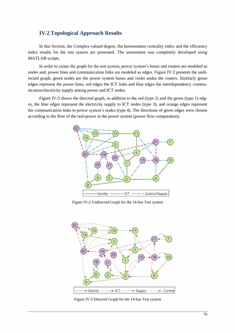
79
IV.2 Topological Approach Results
In this Section, the Complex-valued degree, the betweenness centrality index and the efficiency index results for the test system are presented. The assessment was completely developed using MATLAB scripts.
In order to create the graph for the test system, power system’s buses and routers are modeled as nodes and, power lines and communication links are modeled as edges. Figure IV:2 presents the undi-rected graph; green nodes are the power system buses and violet nodes the routers. Similarly green edges represent the power lines, red edges the ICT links and blue edges the interdependency commu-nication/electricity supply among power and ICT nodes.
Figure IV:3 shows the directed graph, in addition to the red (type 2) and the green (type 1) edg-es, the blue edges represent the electricity supply to ICT nodes (type 3), and orange edges represent the communication links to power system’s nodes (type 4). The directions of green edges were chosen according to the flow of the real-power in the power system (power flow computation).
Figure IV:2 Undirected Graph for the 14-bus Test system
Figure IV:3 Directed Graph for the 14-bus Test system
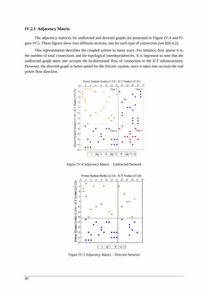
80
IV.2.1 Adjacency Matrix
The adjacency matrices for undirected and directed graphs are presented in Figure IV:4 and Fi-gure IV:5. These figures show four different sections, one for each type of connection (see §III.4.2).
This representation describes the coupled system in many ways. For instance, how sparse it is, the number of total connections and the topological interdependencies. It is important to note that the undirected graph takes into account the bi-directional flow of connection in the ICT infrastructures. However, the directed graph is better suited for the Electric system, since it takes into account the real power flow direction.
Figure IV:4 Adjacency Matrix – Undirected Network
Figure IV:5 Adjacency Matrix – Directed Network
Type 1 Type 3
Type 2 Type 4
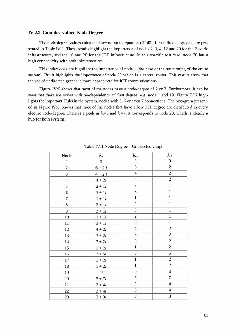
81
IV.2.2 Complex-valued Node Degree
The node degree values calculated according to equation (III.40), for undirected graphs, are pre-sented in Table IV :1. These results highlight the importance of nodes 2, 3, 4, 12 and 20 for the Electric infrastructure, and the 16 and 20 for the ICT infrastructure. In this specific test case, node 20 has a high connectivity with both infrastructures.
This index does not highlight the importance of node 1 (the base of the functioning of the entire system). But it highlights the importance of node 20 which is a central router. This results show that the use of undirected graphs is more appropriate for ICT communications.
Figure IV:6 shows that most of the nodes have a node-degree of 2 or 3. Furthermore, it can be seen that there are nodes with no-dependency of first degree, e.g. node 1 and 19. Figure IV:7 high-lights the important Hubs in the system, nodes with 5, 6 or even 7 connections. The histogram present-ed in Figure IV:8, shows that most of the nodes that have a low ICT degree are distributed in every electric node-degree. There is a peak in ke=6 and kc=7, it corresponds to node 20, which is clearly a hub for both systems.
Table IV :1 Node Degree – Undirected Graph
Node kh keh kch
1 3 3 0
2 6 + 2 i 6 2
3 4 + 2 i 4 2
4 4 + 2i 4 2
5 2 + 1i 2 1
6 3 + 1i 3 1
7 1 + 1i 1 1
8 2 + 1i 2 1
9 3 + 1i 3 1
10 2 + 1i 2 1
11 3 + 1i 3 1
12 4 + 2i 4 2
13 3 + 2i 3 2
14 3 + 2i 3 2
15 1 + 2i 1 2
16 3 + 5i 3 5
17 1 + 2i 1 2
18 1 + 2i 1 2
19 4i 0 4
20 5 + 7i 5 7
21 2 + 4i 2 4
22 3 + 4i 3 4
23 3 + 3i 3 3
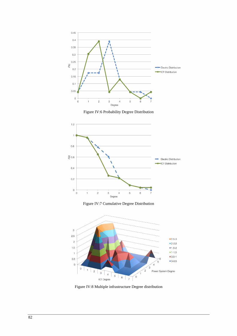
82
Figure IV:6 Probability Degree Distribution
Figure IV:7 Cumulative Degree Distribution
Figure IV:8 Multiple infrastructure Degree distribution

83
The node-degrees according to equations (III.41) and (III.42), for directed graphs, are presented in Table IV :2. In-degree presents how dependent are the nodes to each infrastructure. The Out-degree shows the importance of each node for each infrastructure. In this case, nodes 2 and 14 are highlighted as the most important electric nodes, and nodes 20 and 16 as the most important for the ICT infrastruc-ture. On the other hand, node 19 is the most dependent node in the ICT infrastructure. However, node 2 has dependencies in both infrastructures. For that reason it is considered as the most critical node for the ICT and Electric Infrastructure.
Figure IV:9 shows that there are no-critical hubs since the highest in-degree is 3 for the ICT in-frastructure and 2 for the Electric Infrastructure. In addition, according to Figure IV:10, most of the nodes have a degree 1. In fact, Figure IV:11 shows that most of the nodes have only one connection with the electric and the ICT infrastructure.
Figure IV:12 and Figure IV:13 show that in the ICT infrastructure there are important hubs, having out-degrees of 5 and 6. On the contrary, Electric system has a clear tendency to have only one connection. It is due to the topological properties of Distribution Power Systems.
Figure IV:14 helps to understand the dependencies among and within infrastructures, for in-stance, there is a local maximum for the out-degree 6, but this node has a 0 electric out-degree.
Table IV:2 Node Degree – Directed Graph
Node khin keh
in kchin kh
out kehout kch
out
1 2 2 0 1 1 0
2 2 + 2 i 2 2 3 3 0
3 1 + 2 i 1 2 1 1 0
4 1 + 2 i 1 2 1 1 0
5 1 + 1 i 1 1 1 1 0
6 1 + 1 i 1 1 1 1 0
7 1 i 0 1 1 1 0
8 1 + 1 i 1 1 2 2 0
9 1 + 1 i 1 1 1 1 0
10 1 i 0 1 2 2 0
11 1 + 1 i 1 1 1 1 0
12 1 + 2 i 1 2 1 1 0
13 2 i 0 2 1 1 0
14 2 i 0 2 3 3 0
15 1 1 1 2 i 0 2
16 1 + 1 i 1 1 4 i 0 4
17 1 1 1 2 i 0 2
18 1 1 1 2 i 0 2
19 1 + 3 i 1 3 1 i 0 1
20 1 + 1 i 1 1 6 i 0 6
21 1 + 1 i 1 1 3 i 0 3
22 1 + 1 i 1 1 3 i 0 3
23 0 0 0 3 i 0 3
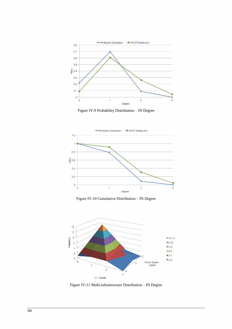
84
Figure IV:9 Probability Distribution – IN Degree
Figure IV:10 Cumulative Distribution – IN Degree
Figure IV:11 Multi-infrastructure Distribution – IN Degree
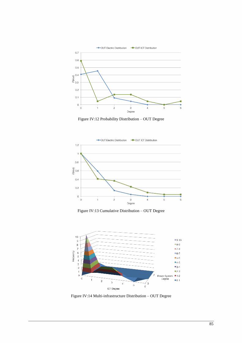
85
Figure IV:12 Probability Distribution – OUT Degree
Figure IV:13 Cumulative Distribution – OUT Degree
Figure IV:14 Multi-infrastructure Distribution – OUT Degree
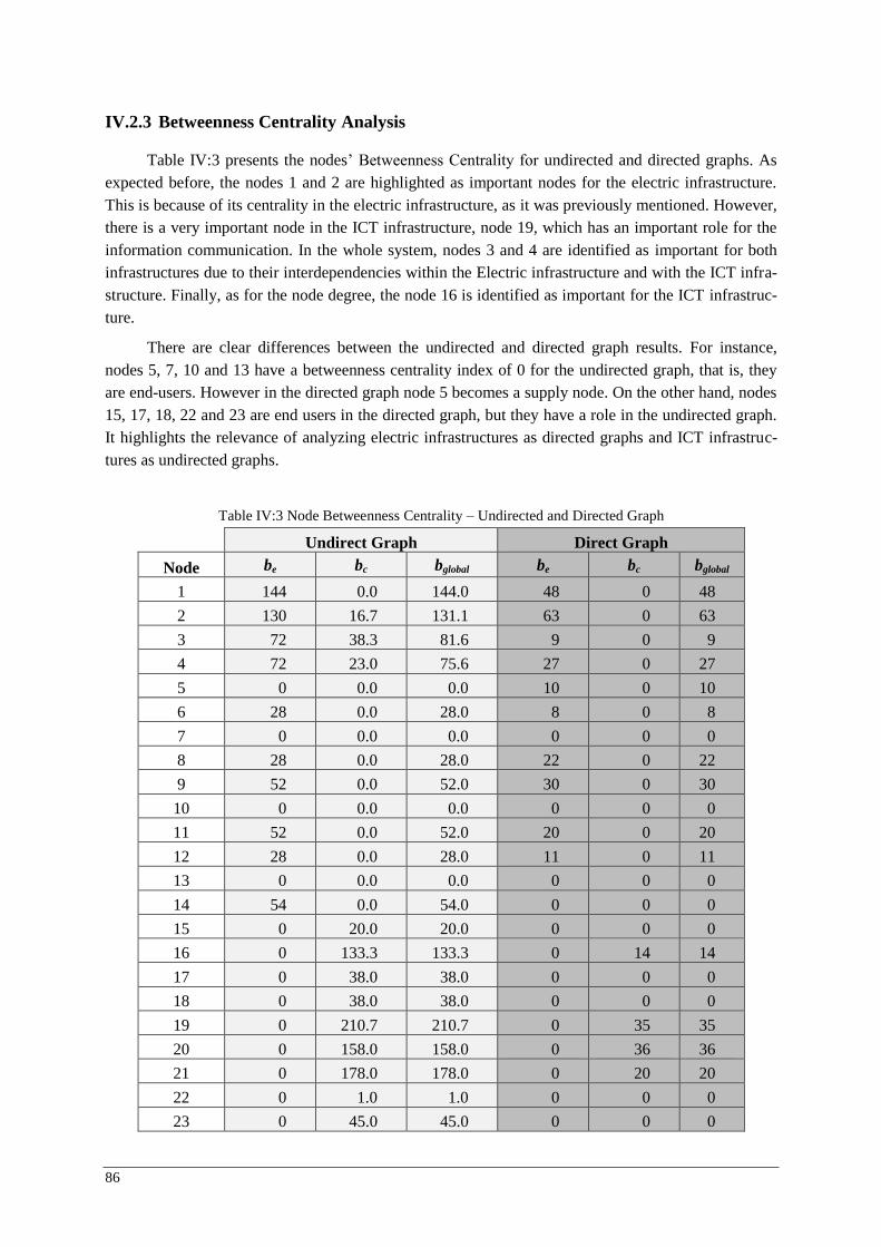
86
IV.2.3 Betweenness Centrality Analysis
Table IV :3 presents the nodes’ Betweenness Centrality for undirected and directed graphs. As expected before, the nodes 1 and 2 are highlighted as important nodes for the electric infrastructure. This is because of its centrality in the electric infrastructure, as it was previously mentioned. However, there is a very important node in the ICT infrastructure, node 19, which has an important role for the information communication. In the whole system, nodes 3 and 4 are identified as important for both infrastructures due to their interdependencies within the Electric infrastructure and with the ICT infra-structure. Finally, as for the node degree, the node 16 is identified as important for the ICT infrastruc-ture.
There are clear differences between the undirected and directed graph results. For instance, nodes 5, 7, 10 and 13 have a betweenness centrality index of 0 for the undirected graph, that is, they are end-users. However in the directed graph node 5 becomes a supply node. On the other hand, nodes 15, 17, 18, 22 and 23 are end users in the directed graph, but they have a role in the undirected graph. It highlights the relevance of analyzing electric infrastructures as directed graphs and ICT infrastruc-tures as undirected graphs.
Table IV:3 Node Betweenness Centrality – Undirected and Directed Graph
Undirect Graph Direct Graph
Node be bc bglobal be bc bglobal
1 144 0.0 144.0 48 0 48
2 130 16.7 131.1 63 0 63
3 72 38.3 81.6 9 0 9
4 72 23.0 75.6 27 0 27
5 0 0.0 0.0 10 0 10
6 28 0.0 28.0 8 0 8
7 0 0.0 0.0 0 0 0
8 28 0.0 28.0 22 0 22
9 52 0.0 52.0 30 0 30
10 0 0.0 0.0 0 0 0
11 52 0.0 52.0 20 0 20
12 28 0.0 28.0 11 0 11
13 0 0.0 0.0 0 0 0
14 54 0.0 54.0 0 0 0
15 0 20.0 20.0 0 0 0
16 0 133.3 133.3 0 14 14
17 0 38.0 38.0 0 0 0
18 0 38.0 38.0 0 0 0
19 0 210.7 210.7 0 35 35
20 0 158.0 158.0 0 36 36
21 0 178.0 178.0 0 20 20
22 0 1.0 1.0 0 0 0
23 0 45.0 45.0 0 0 0
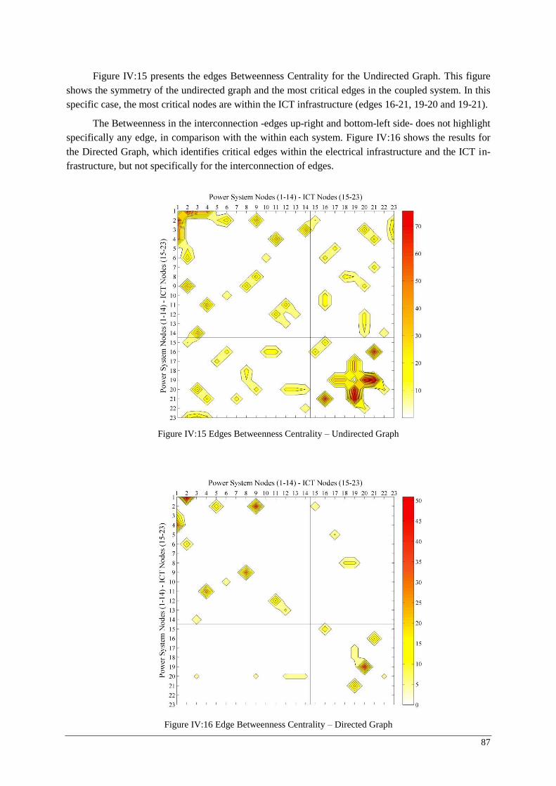
87
Figure IV:15 presents the edges Betweenness Centrality for the Undirected Graph. This figure shows the symmetry of the undirected graph and the most critical edges in the coupled system. In this specific case, the most critical nodes are within the ICT infrastructure (edges 16-21, 19-20 and 19-21).
The Betweenness in the interconnection -edges up-right and bottom-left side- does not highlight specifically any edge, in comparison with the within each system. Figure IV:16 shows the results for the Directed Graph, which identifies critical edges within the electrical infrastructure and the ICT in-frastructure, but not specifically for the interconnection of edges.
Figure IV:15 Edges Betweenness Centrality – Undirected Graph
Figure IV:16 Edge Betweenness Centrality – Directed Graph

88
IV.2.4 Efficiency
Table IV :4 presents the efficiency results after removing each node in the coupled test system. The nodes 1, 2, and 20 are identified as critical nodes within their own infrastructures. However, nodes 15 and 19 are recognized as important nodes for both infrastructures, having an impact in the efficien-cy of both infrastructures. Figure IV:17 and Figure IV:18 show the same results for a better interpreta-tion.
The highest impact for the undirected graph is 60% (node 2) and 57% for the directed graph (node 2 as well). That means that even in the case N-1, there are still topological paths to ensure the continuity of service. This does not mean that physically the system will continue to work, but that there are options to reconfigure the system. Nodes 8, 9 and 14 are identified, for the first time, as criti-cal within the Electric infrastructure.
Table IV:4 Vertices efficiency Undirected and Directed Graph
UNDIRECTED GRAPH DIRECTED GRAPH
Electric Efficiency ICT Efficiency Electric Efficiency ICT Efficiency Node Ee ΔEe Ec ΔEc Ee ΔEe Ec ΔEc
Normal State 0.2327
0.4062
0.1473
0.2533 1 0.1384 41% 0.4062 0% 0.0991 33% 0.2533 0%
2 0.0927 60% 0.3729 8% 0.0635 57% 0.2374 6%
3 0.1717 26% 0.3639 10% 0.1333 10% 0.2220 12%
4 0.1919 18% 0.3688 9% 0.1237 16% 0.2308 9%
5 0.1862 20% 0.3792 7% 0.1185 20% 0.2454 3%
6 0.1864 20% 0.3782 7% 0.1289 12% 0.2414 5%
7 0.2247 3% 0.3751 8% 0.1394 5% 0.2388 6%
8 0.1637 30% 0.3792 7% 0.0912 38% 0.2454 3%
9 0.1678 28% 0.3762 7% 0.1071 27% 0.2299 9%
10 0.1922 17% 0.3782 7% 0.1316 11% 0.2414 5%
11 0.2053 12% 0.3782 7% 0.1315 11% 0.2414 5%
12 0.2160 7% 0.3722 8% 0.1377 7% 0.2220 12%
13 0.2250 3% 0.3722 8% 0.1429 3% 0.2220 12%
14 0.1652 29% 0.3722 8% 0.1252 15% 0.2220 12%
15 0.1914 18% 0.3669 10% 0.1166 21% 0.2202 13%
16 0.2026 13% 0.2943 28% 0.1394 5% 0.1865 26%
17 0.1993 14% 0.3505 14% 0.1185 20% 0.2321 8%
18 0.2026 13% 0.3505 14% 0.1193 19% 0.2321 8%
19 0.2026 13% 0.2664 34% 0.1193 19% 0.1759 31%
20 0.2027 13% 0.2481 39% 0.1394 5% 0.1362 46%
21 0.2247 3% 0.3087 24% 0.1394 5% 0.1931 24%
22 0.2027 13% 0.3598 11% 0.1394 5% 0.2295 9%
23 0.2327 0% 0.3573 12% 0.1473 0% 0.2295 9%
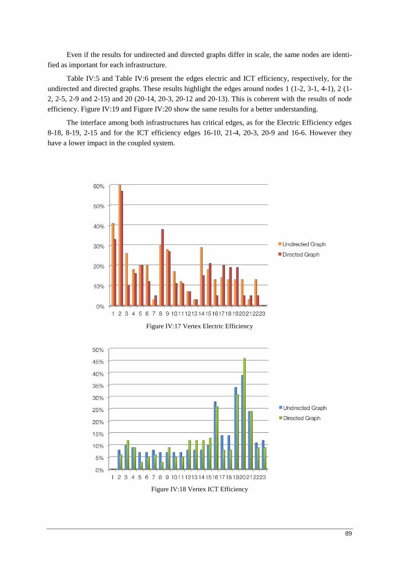
89
Even if the results for undirected and directed graphs differ in scale, the same nodes are identi-fied as important for each infrastructure.
Table IV :5 and Table IV :6 present the edges electric and ICT efficiency, respectively, for the undirected and directed graphs. These results highlight the edges around nodes 1 (1-2, 3-1, 4-1), 2 (1-2, 2-5, 2-9 and 2-15) and 20 (20-14, 20-3, 20-12 and 20-13). This is coherent with the results of node efficiency. Figure IV:19 and Figure IV:20 show the same results for a better understanding.
The interface among both infrastructures has critical edges, as for the Electric Efficiency edges 8-18, 8-19, 2-15 and for the ICT efficiency edges 16-10, 21-4, 20-3, 20-9 and 16-6. However they have a lower impact in the coupled system.
Figure IV:17 Vertex Electric Efficiency
Figure IV:18 Vertex ICT Efficiency
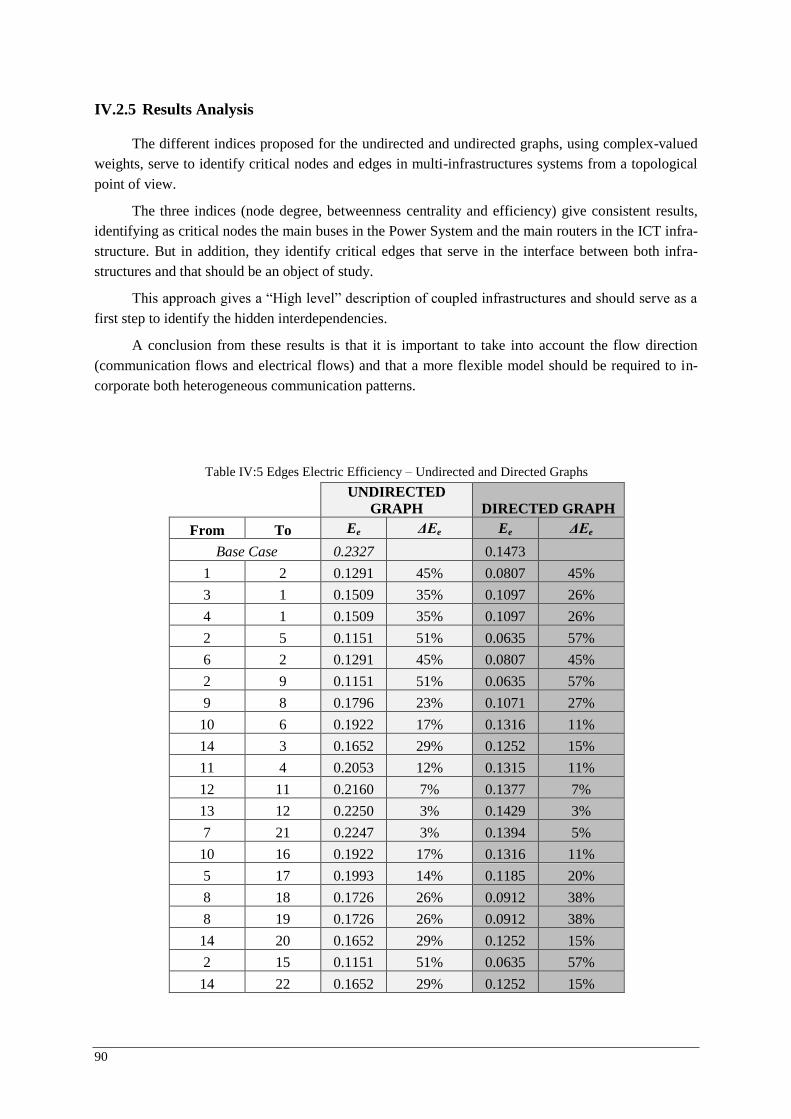
90
IV.2.5 Results Analysis
The different indices proposed for the undirected and undirected graphs, using complex-valued weights, serve to identify critical nodes and edges in multi-infrastructures systems from a topological point of view.
The three indices (node degree, betweenness centrality and efficiency) give consistent results, identifying as critical nodes the main buses in the Power System and the main routers in the ICT infra-structure. But in addition, they identify critical edges that serve in the interface between both infra-structures and that should be an object of study.
This approach gives a “High level” description of coupled infrastructures and should serve as a first step to identify the hidden interdependencies.
A conclusion from these results is that it is important to take into account the flow direction (communication flows and electrical flows) and that a more flexible model should be required to in-corporate both heterogeneous communication patterns.
Table IV:5 Edges Electric Efficiency – Undirected and Directed Graphs
UNDIRECTED
GRAPH DIRECTED GRAPH
From To Ee ΔEe Ee ΔEe
Base Case 0.2327 0.1473
1 2 0.1291 45% 0.0807 45%
3 1 0.1509 35% 0.1097 26%
4 1 0.1509 35% 0.1097 26%
2 5 0.1151 51% 0.0635 57%
6 2 0.1291 45% 0.0807 45%
2 9 0.1151 51% 0.0635 57%
9 8 0.1796 23% 0.1071 27%
10 6 0.1922 17% 0.1316 11%
14 3 0.1652 29% 0.1252 15%
11 4 0.2053 12% 0.1315 11%
12 11 0.2160 7% 0.1377 7%
13 12 0.2250 3% 0.1429 3%
7 21 0.2247 3% 0.1394 5%
10 16 0.1922 17% 0.1316 11%
5 17 0.1993 14% 0.1185 20%
8 18 0.1726 26% 0.0912 38%
8 19 0.1726 26% 0.0912 38%
14 20 0.1652 29% 0.1252 15%
2 15 0.1151 51% 0.0635 57%
14 22 0.1652 29% 0.1252 15%
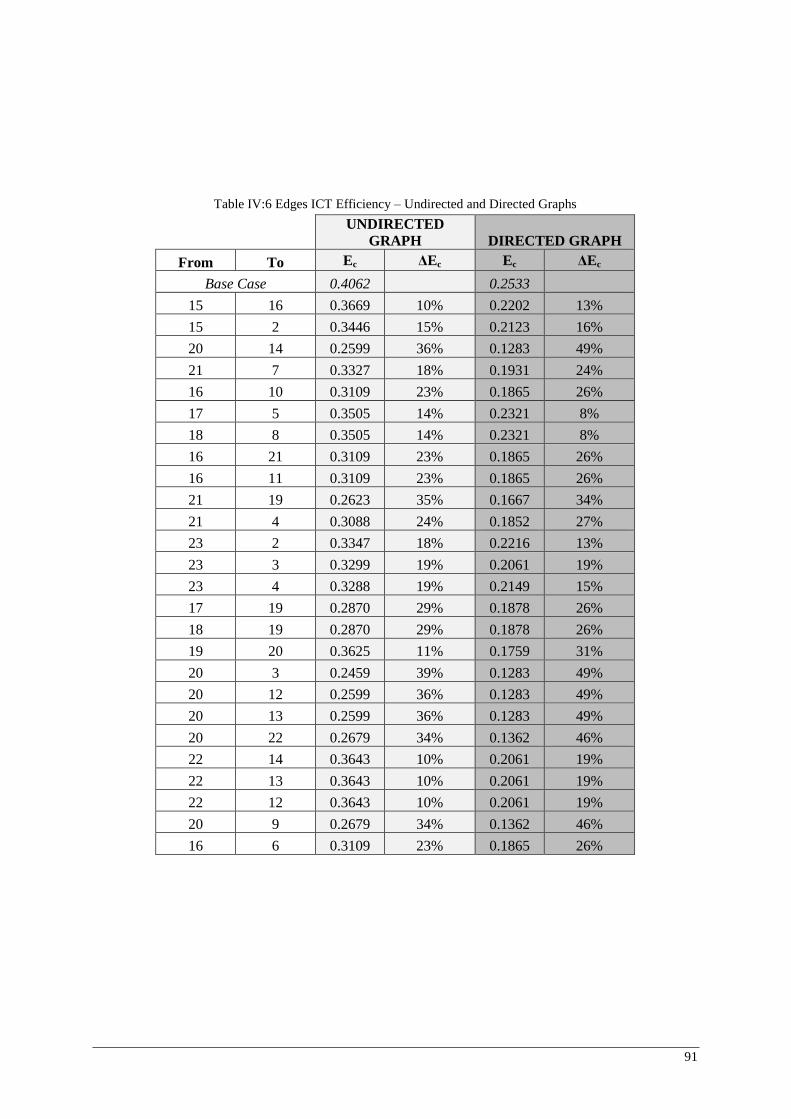
91
Table IV:6 Edges ICT Efficiency – Undirected and Directed Graphs
UNDIRECTED
GRAPH DIRECTED GRAPH
From To Ec ΔEc Ec ΔEc
Base Case 0.4062 0.2533
15 16 0.3669 10% 0.2202 13%
15 2 0.3446 15% 0.2123 16%
20 14 0.2599 36% 0.1283 49%
21 7 0.3327 18% 0.1931 24%
16 10 0.3109 23% 0.1865 26%
17 5 0.3505 14% 0.2321 8%
18 8 0.3505 14% 0.2321 8%
16 21 0.3109 23% 0.1865 26%
16 11 0.3109 23% 0.1865 26%
21 19 0.2623 35% 0.1667 34%
21 4 0.3088 24% 0.1852 27%
23 2 0.3347 18% 0.2216 13%
23 3 0.3299 19% 0.2061 19%
23 4 0.3288 19% 0.2149 15%
17 19 0.2870 29% 0.1878 26%
18 19 0.2870 29% 0.1878 26%
19 20 0.3625 11% 0.1759 31%
20 3 0.2459 39% 0.1283 49%
20 12 0.2599 36% 0.1283 49%
20 13 0.2599 36% 0.1283 49%
20 22 0.2679 34% 0.1362 46%
22 14 0.3643 10% 0.2061 19%
22 13 0.3643 10% 0.2061 19%
22 12 0.3643 10% 0.2061 19%
20 9 0.2679 34% 0.1362 46%
16 6 0.3109 23% 0.1865 26%
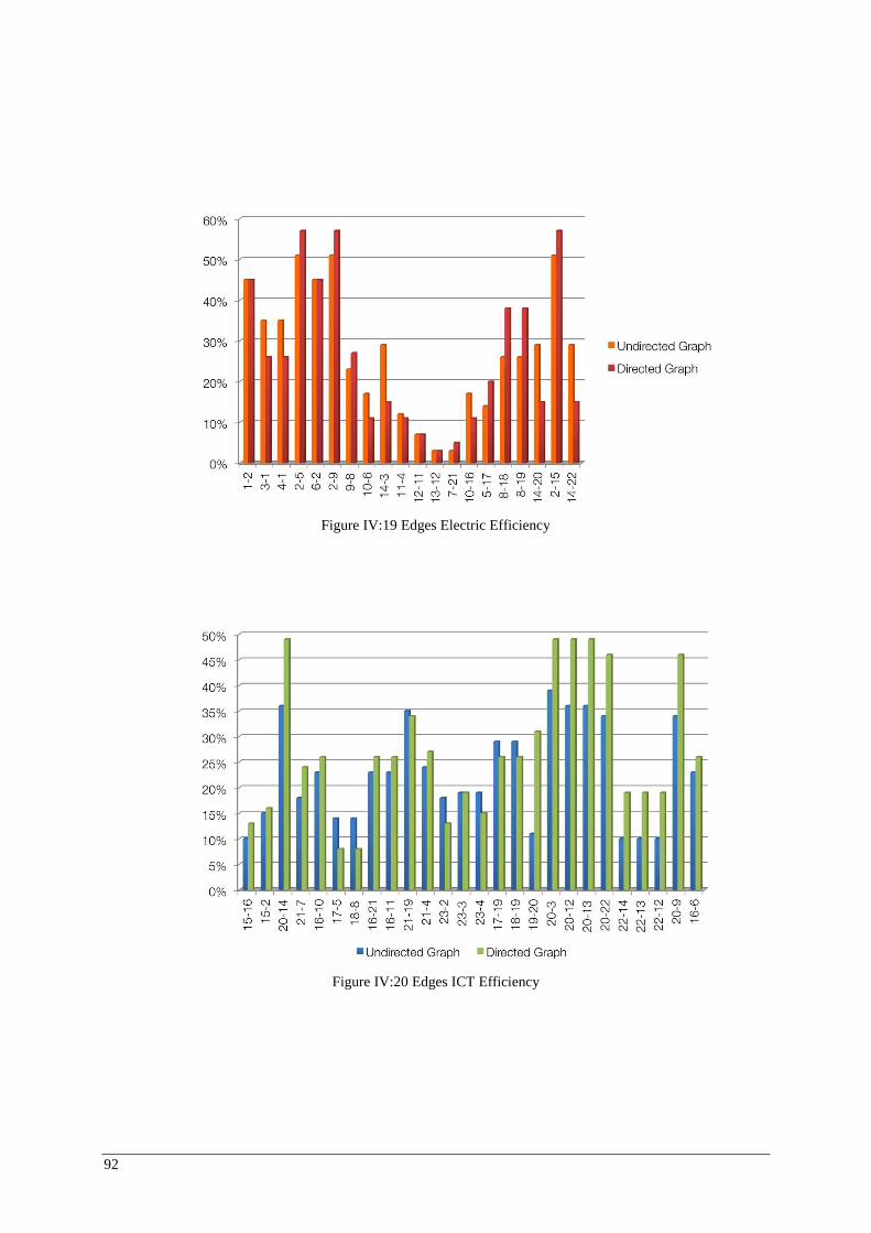
92
Figure IV:19 Edges Electric Efficiency
Figure IV:20 Edges ICT Efficiency
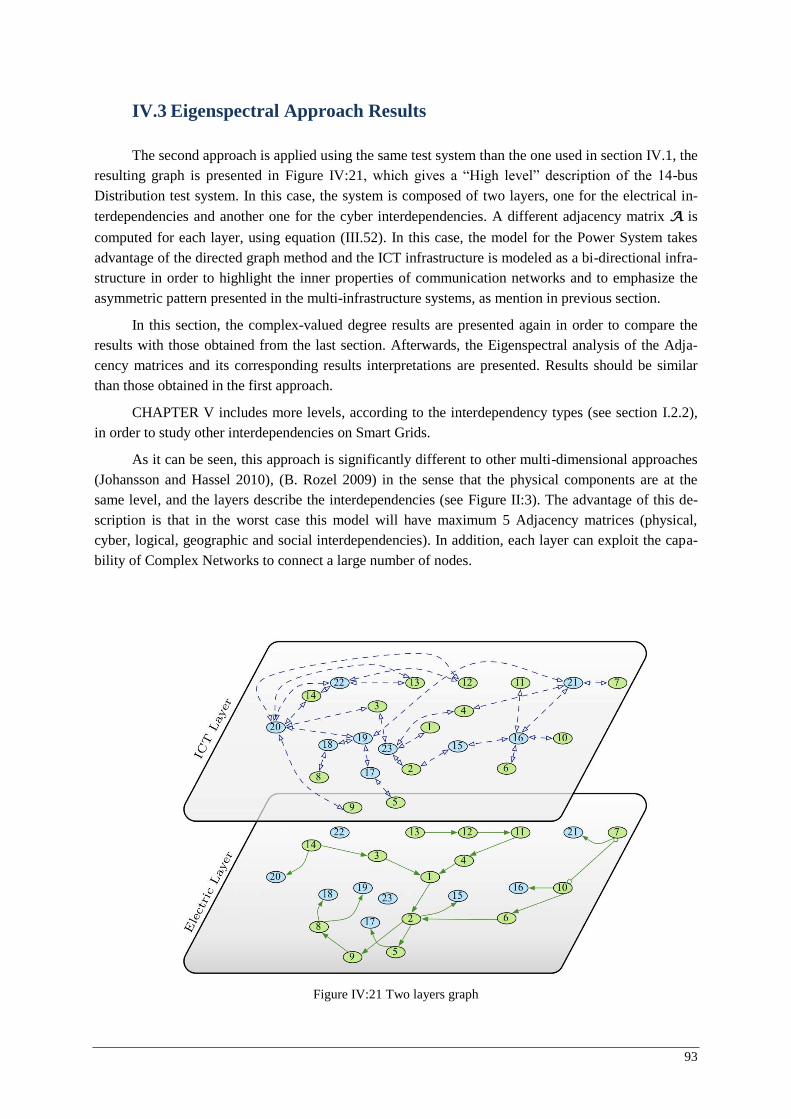
93
IV.3 Eigenspectral Approach Results
The second approach is applied using the same test system than the one used in section IV.1, the resulting graph is presented in Figure IV:21, which gives a “High level” description of the 14-bus Distribution test system. In this case, the system is composed of two layers, one for the electrical in-
terdependencies and another one for the cyber interdependencies. A different adjacency matrix A is
computed for each layer, using equation (III.52). In this case, the model for the Power System takes advantage of the directed graph method and the ICT infrastructure is modeled as a bi-directional infra-structure in order to highlight the inner properties of communication networks and to emphasize the asymmetric pattern presented in the multi-infrastructure systems, as mention in previous section.
In this section, the complex-valued degree results are presented again in order to compare the results with those obtained from the last section. Afterwards, the Eigenspectral analysis of the Adja-cency matrices and its corresponding results interpretations are presented. Results should be similar than those obtained in the first approach.
CHAPTER V includes more levels, according to the interdependency types (see section I.2.2), in order to study other interdependencies on Smart Grids.
As it can be seen, this approach is significantly different to other multi-dimensional approaches (Johansson and Hassel 2010), (B. Rozel 2009) in the sense that the physical components are at the same level, and the layers describe the interdependencies (see Figure II :3). The advantage of this de-scription is that in the worst case this model will have maximum 5 Adjacency matrices (physical, cyber, logical, geographic and social interdependencies). In addition, each layer can exploit the capa-bility of Complex Networks to connect a large number of nodes.
Figure IV:21 Two layers graph
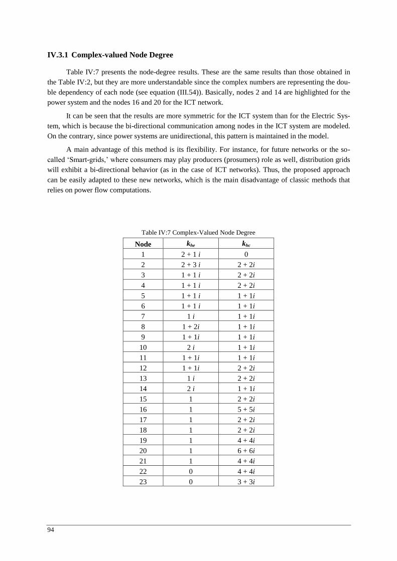
94
IV.3.1 Complex-valued Node Degree
Table IV :7 presents the node-degree results. These are the same results than those obtained in the Table IV :2, but they are more understandable since the complex numbers are representing the dou-ble dependency of each node (see equation (III.54)). Basically, nodes 2 and 14 are highlighted for the power system and the nodes 16 and 20 for the ICT network.
It can be seen that the results are more symmetric for the ICT system than for the Electric Sys-tem, which is because the bi-directional communication among nodes in the ICT system are modeled. On the contrary, since power systems are unidirectional, this pattern is maintained in the model.
A main advantage of this method is its flexibility. For instance, for future networks or the so-called ‘Smart-grids,’ where consumers may play producers (prosumers) role as well, distribution grids will exhibit a bi-directional behavior (as in the case of ICT networks). Thus, the proposed approach can be easily adapted to these new networks, which is the main disadvantage of classic methods that relies on power flow computations.
Table IV:7 Complex-Valued Node Degree
Node khe khc
1 2 + 1 i 0
2 2 + 3 i 2 + 2i
3 1 + 1 i 2 + 2i
4 1 + 1 i 2 + 2i
5 1 + 1 i 1 + 1i
6 1 + 1 i 1 + 1i
7 1 i 1 + 1i
8 1 + 2i 1 + 1i
9 1 + 1i 1 + 1i
10 2 i 1 + 1i
11 1 + 1i 1 + 1i
12 1 + 1i 2 + 2i
13 1 i 2 + 2i
14 2 i 1 + 1i
15 1 2 + 2i
16 1 5 + 5i
17 1 2 + 2i
18 1 2 + 2i
19 1 4 + 4i
20 1 6 + 6i
21 1 4 + 4i
22 0 4 + 4i
23 0 3 + 3i
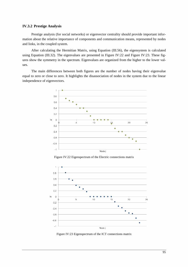
95
IV.3.2 Prestige Analysis
Prestige analysis (for social networks) or eigenvector centrality should provide important infor-mation about the relative importance of components and communication means, represented by nodes and links, in the coupled system.
After calculating the Hermitian Matrix, using Equation (III.56), the eigensystem is calculated using Equation (III.32). The eigenvalues are presented in Figure IV:22 and Figure IV:23. These fig-ures show the symmetry in the spectrum. Eigenvalues are organized from the higher to the lower val-ues.
The main differences between both figures are the number of nodes having their eigenvalue equal to zero or close to zero. It highlights the disassociation of nodes in the system due to the linear independence of eigenvectors.
Figure IV:22 Eigenspectrum of the Electric connections matrix
Figure IV:23 Eigenspectrum of the ICT connections matrix
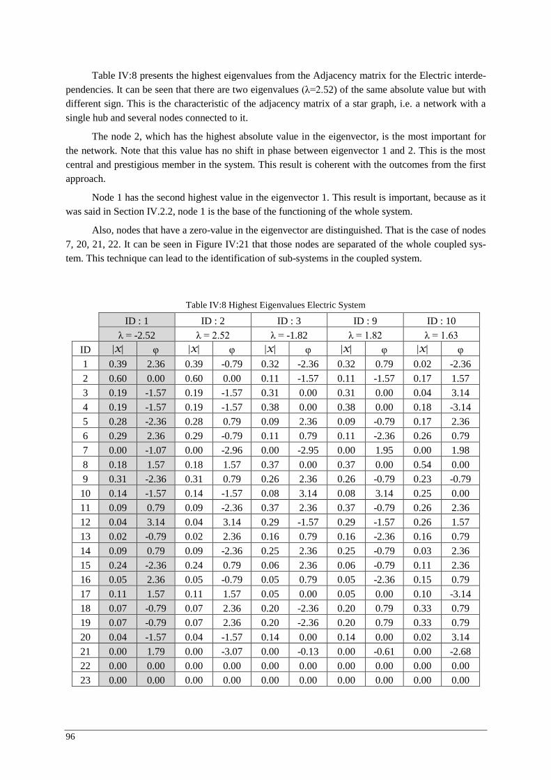
96
Table IV :8 presents the highest eigenvalues from the Adjacency matrix for the Electric interde-pendencies. It can be seen that there are two eigenvalues (λ=2.52) of the same absolute value but with different sign. This is the characteristic of the adjacency matrix of a star graph, i.e. a network with a single hub and several nodes connected to it.
The node 2, which has the highest absolute value in the eigenvector, is the most important for the network. Note that this value has no shift in phase between eigenvector 1 and 2. This is the most central and prestigious member in the system. This result is coherent with the outcomes from the first approach.
Node 1 has the second highest value in the eigenvector 1. This result is important, because as it was said in Section IV.2.2, node 1 is the base of the functioning of the whole system.
Also, nodes that have a zero-value in the eigenvector are distinguished. That is the case of nodes 7, 20, 21, 22. It can be seen in Figure IV:21 that those nodes are separated of the whole coupled sys-tem. This technique can lead to the identification of sub-systems in the coupled system.
Table IV:8 Highest Eigenvalues Electric System
ID : 1 ID : 2 ID : 3 ID : 9 ID : 10
λ = -2.52 λ = 2.52 λ = -1.82 λ = 1.82 λ = 1.63
ID |x| φ |x| φ |x| φ |x| φ |x| φ
1 0.39 2.36 0.39 -0.79 0.32 -2.36 0.32 0.79 0.02 -2.36
2 0.60 0.00 0.60 0.00 0.11 -1.57 0.11 -1.57 0.17 1.57
3 0.19 -1.57 0.19 -1.57 0.31 0.00 0.31 0.00 0.04 3.14
4 0.19 -1.57 0.19 -1.57 0.38 0.00 0.38 0.00 0.18 -3.14
5 0.28 -2.36 0.28 0.79 0.09 2.36 0.09 -0.79 0.17 2.36
6 0.29 2.36 0.29 -0.79 0.11 0.79 0.11 -2.36 0.26 0.79
7 0.00 -1.07 0.00 -2.96 0.00 -2.95 0.00 1.95 0.00 1.98
8 0.18 1.57 0.18 1.57 0.37 0.00 0.37 0.00 0.54 0.00
9 0.31 -2.36 0.31 0.79 0.26 2.36 0.26 -0.79 0.23 -0.79
10 0.14 -1.57 0.14 -1.57 0.08 3.14 0.08 3.14 0.25 0.00
11 0.09 0.79 0.09 -2.36 0.37 2.36 0.37 -0.79 0.26 2.36
12 0.04 3.14 0.04 3.14 0.29 -1.57 0.29 -1.57 0.26 1.57
13 0.02 -0.79 0.02 2.36 0.16 0.79 0.16 -2.36 0.16 0.79
14 0.09 0.79 0.09 -2.36 0.25 2.36 0.25 -0.79 0.03 2.36
15 0.24 -2.36 0.24 0.79 0.06 2.36 0.06 -0.79 0.11 2.36
16 0.05 2.36 0.05 -0.79 0.05 0.79 0.05 -2.36 0.15 0.79
17 0.11 1.57 0.11 1.57 0.05 0.00 0.05 0.00 0.10 -3.14
18 0.07 -0.79 0.07 2.36 0.20 -2.36 0.20 0.79 0.33 0.79
19 0.07 -0.79 0.07 2.36 0.20 -2.36 0.20 0.79 0.33 0.79
20 0.04 -1.57 0.04 -1.57 0.14 0.00 0.14 0.00 0.02 3.14
21 0.00 1.79 0.00 -3.07 0.00 -0.13 0.00 -0.61 0.00 -2.68
22 0.00 0.00 0.00 0.00 0.00 0.00 0.00 0.00 0.00 0.00
23 0.00 0.00 0.00 0.00 0.00 0.00 0.00 0.00 0.00 0.00
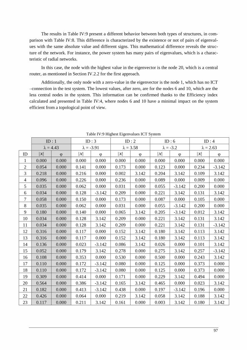
97
The results in Table IV :9 present a different behavior between both types of structures, in com-parison with Table IV :8. This difference is characterized by the existence or not of pairs of eigenval-ues with the same absolute value and different signs. This mathematical difference reveals the struc-ture of the network. For instance, the power system has many pairs of eigenvalues, which is a charac-teristic of radial networks.
In this case, the node with the highest value in the eigenvector is the node 20, which is a central router, as mentioned in Section IV.2.2 for the first approach.
Additionally, the only node with a zero-value in the eigenvector is the node 1, which has no ICT –connection in the test system. The lowest values, after zero, are for the nodes 6 and 10, which are the less central nodes in the system. This information can be confirmed thanks to the Efficiency index calculated and presented in Table IV :4, where nodes 6 and 10 have a minimal impact on the system efficient from a topological point of view.
Table IV:9 Highest Eigenvalues ICT System
ID : 1 ID : 3 ID : 2 ID : 6 ID : 4
λ = 4.43 λ = -3.91 λ = 3.58 λ = -3.2 λ = 2.63
ID |x| φ |x| φ |x| φ |x| φ |x| φ
1 0.000 0.000 0.000 0.000 0.000 0.000 0.000 0.000 0.000 0.000
2 0.054 0.000 0.141 0.000 0.173 0.000 0.123 0.000 0.234 -3.142
3 0.218 0.000 0.216 0.000 0.002 3.142 0.204 3.142 0.109 3.142
4 0.096 0.000 0.226 0.000 0.236 0.000 0.089 0.000 0.009 0.000
5 0.035 0.000 0.062 0.000 0.031 0.000 0.055 -3.142 0.200 0.000
6 0.034 0.000 0.128 -3.142 0.209 0.000 0.221 3.142 0.131 3.142
7 0.058 0.000 0.150 0.000 0.173 0.000 0.087 0.000 0.105 0.000
8 0.035 0.000 0.062 0.000 0.031 0.000 0.055 -3.142 0.200 0.000
9 0.180 0.000 0.140 0.000 0.065 3.142 0.205 -3.142 0.012 3.142
10 0.034 0.000 0.128 3.142 0.209 0.000 0.221 3.142 0.131 3.142
11 0.034 0.000 0.128 3.142 0.209 0.000 0.221 3.142 0.131 -3.142
12 0.316 0.000 0.117 0.000 0.152 3.142 0.180 3.142 0.113 3.142
13 0.316 0.000 0.117 0.000 0.152 3.142 0.180 3.142 0.113 3.142
14 0.136 0.000 0.023 -3.142 0.086 3.142 0.026 0.000 0.101 3.142
15 0.052 0.000 0.179 3.142 0.278 0.000 0.275 3.142 0.257 -3.142
16 0.108 0.000 0.353 0.000 0.530 0.000 0.500 0.000 0.243 3.142
17 0.110 0.000 0.172 -3.142 0.080 0.000 0.125 0.000 0.373 0.000
18 0.110 0.000 0.172 -3.142 0.080 0.000 0.125 0.000 0.373 0.000
19 0.309 0.000 0.414 0.000 0.171 0.000 0.229 3.142 0.494 0.000
20 0.564 0.000 0.386 -3.142 0.165 3.142 0.465 0.000 0.023 3.142
21 0.182 0.000 0.413 -3.142 0.438 0.000 0.197 -3.142 0.196 0.000
22 0.426 0.000 0.064 0.000 0.219 3.142 0.058 3.142 0.188 3.142
23 0.117 0.000 0.211 3.142 0.161 0.000 0.003 3.142 0.180 3.142
98
IV.4 Conclusions
This Chapter presented the application of the approaches proposed in CHAPTER III to model coupled infrastructures, in this case a Distribution Network with its surrounding Communication net-work.
The first approach studies the topology of the system supported by a modification of the classi-cal properties of graph theory, such as node-degree, betweenness centrality and efficiency. The modi-fication consisted in the application of complex-weighted adjacency matrices and two-layer analysis, according to the interdependencies. These indices served to identify critical nodes and edges in multi-infrastructures systems from a topological point of view.
Results give coherent results, identifying as critical nodes the main buses in the Power System and the main Routers in the ICT infrastructure. But in addition, they reveal critical edges that serve in the interface between both infrastructures. In addition, these results highlight the importance to model coupled systems as undirected and directed graphs, in order to evaluate the heterogeneous communica-tion patterns in each infrastructure.
The second approach, analyzes the Eigensystem of the complex-weighted adjacency matrix that represent the coupled infrastructures. In order to facilitate the interpretation of results, the complex-weighted adjacency matrix is transformed to the Hilbert Space using Hermitian matrices. As a result, eigenvalues from this system are all real-values, where the eigenvectors from the highest eigenvalue is interpreted as an index of importance and relevance of the node in the coupled system.
This approach improves some weaknesses of the first approach, such as the bi-directional com-munication in each infrastructure. Therefore, both systems can include bi-directional edges, which should serve to study different types of infrastructures.
Some of the main advantages of the proposed approaches are:
The application of complex numbers added flexibility to the classical definitions and prop-erties of complex networks. Therefore, new indices can be developed to perform vulnerabil-ity assessment and interdependencies modeling of coupled infrastructures, despite their in-herent differences.
These approaches can be applied to a wide range of coupled heterogeneous systems.
Even if this Chapter depicts and analysis taking into account physical and cyber interde-pendencies, many other interdependencies types can be applied, which will be explored in CHAPTER V.
Due to the availability of fast algorithms to study Complex Networks, the CPU Time re-quired to model large coupled infrastructures is very low.
Scalability is possible using complex networks and generally it will not affect the computa-tional processing time.
99
CHAPTER V
System-of-Systems vision of Coupled Infrastructures
The secret of all victory lies in the organization of the non-obvious
Marcus Aurelius
TABLE OF CONTENTS
V.1 INTRODUCTION ............................................................................................................ 100
V.2 “LOW-LEVEL” SYSTEM DESCRIPTION ANALYSIS ........................................................ 101
V.2.1 Test system – HV/MV Substation .................................................................. 101
V.2.2 Complex-networks modeling methodology .................................................... 104
V.2.3 Results “Low level” description ..................................................................... 105
V.3 INTEGRATION OF “LOW LEVEL” AND “HIGH LEVEL” SYSTEM DESCRIPTION .............. 107
V.3.1 Methodology ................................................................................................... 107
V.3.2 Test case .......................................................................................................... 108
V.4 SMART-GRIDS: A SGAM-BASED SYSTEM-OF-SYSTEMS VISION ................................. 112
V.4.1 Smart Grid Architecture Model (SGAM) ...................................................... 112
V.4.1.1 SGAM: Domains ............................................................................. 113
V.4.1.2 SGAM: Zones .................................................................................. 113
V.4.1.3 SGAM: Interoperability Layers ....................................................... 113
V.4.1.4 SGAM: Architecture........................................................................ 114
V.4.2 Complex Networks modeling ......................................................................... 114
V.4.2.1 Step 1: High level system Description ............................................ 114
V.4.2.2 Step 2: Low Level system Description ............................................ 114
V.4.2.3 Step 3: SoS vision of Smart Grids. .................................................. 115
V.5 SUMMARY .................................................................................................................... 115
Abstract
System-of-Systems approach aims at studying as a whole the different components of multiple infrastruc-
ture systems. This has been called as well: Global Vision of Systems. This analysis is very relevant in order to
understand the behavior of complex systems, particularly, future power distribution systems or ‘Smart Grids’. SGAM is a standardized model proposed by Siemens and standardized by CENELEC and the European Com-
100
mission in order to set a common vision of these grids. This chapter proposes a “Low level” system description
analysis and an integration with “High level” system description analysis in order to create a methodology for
modeling Smart-Grids, based on the SGAM reference.
V.1 Introduction
System of Systems (SoS) Engineering is a discipline that focuses on multiple integrated com-plex systems (Keating, et al. 2003), including cross-system interdependencies. In other words, this discipline studies the Big Picture of Critical Infrastructures. It is believed that it was originated from the System thinking theory (Boardman and Saucer 2008) and evolved due to the rapidly increasing complexity of coupled infrastructures (Gorod, Sauser and Boardman 2008).
Nowadays, this theory has evolved to a Global Systems Science (Jaeger, et al. 2013) that de-fines the complex systems as: Systems that are composed of different heterogeneous parts that include hierarchies, their different parts are coupled and their parts represent different space scales and evolve at different time scales.
It is important to differentiate Systems-of-Subsystems and Systems-of-Systems. On the one hand, in a System-of-Subsystems there is a centralized control, the connectivity is platform-centric, i.e. high connectivity within subsystems and low connectivity among subsystems, and its different parts are homogeneous and have a hierarchy. On the other hand, System-of-Systems is composed of hetero-geneous, autonomous and independent systems, with a decentralized control, and most of the behav-iors are not foreseen (Sauser, Boardman and Gorod 2008).
Critical Infrastructures are seen as a large System-of-Systems, where security issues demands a study of their interdependencies in its entirety (Zolesio 2010). CHAPTER III and CHAPTER IV pre-sented an analysis of two layers physical and cyber of a distribution network, this analysis is called “High level” system description analysis since it describes the system as a whole. However, in that approach some nodes represented a whole system, e.g. a substation. Therefore, in order to expand the proposed approach and to include a “Low level analysis,” this Chapter demonstrates the application of “Low level” system description analysis and applies the Eigenspectral analysis to study the substation interdependencies as an example.
Finally, in order to have the big picture of the whole coupled system; it is proposed a methodol-ogy to model Smart Grids, based in the SGAM reference (Smart Grid Architecture Model). SGAM was developed in 2012 to define the different layers that compose a Smart Grid and to describe their interplays (CEN-CENELEC-ETSI 2012). The proposed methodology in this dissertation integrates several interdependency types. As a result, a new model to study the vulnerabilities and interdepend-encies of power systems, including substations and distributed energy resources is obtained.
The main body of this chapter is divided into four parts; Section V.2 presents the “Low Level” system description analysis as an approach to the System-of-Systems Engineering view of Distribution Networks. In this section the PREDIS Platform is presented as a test system. Section V.3 describes de integration of “Low level” system description and “High-level” system description. Section V.4 intro-duces the SGAM definition and the resulting methodology to model the interdependencies of Smart Grids. Finally, Section V.5 summarizes and concludes.
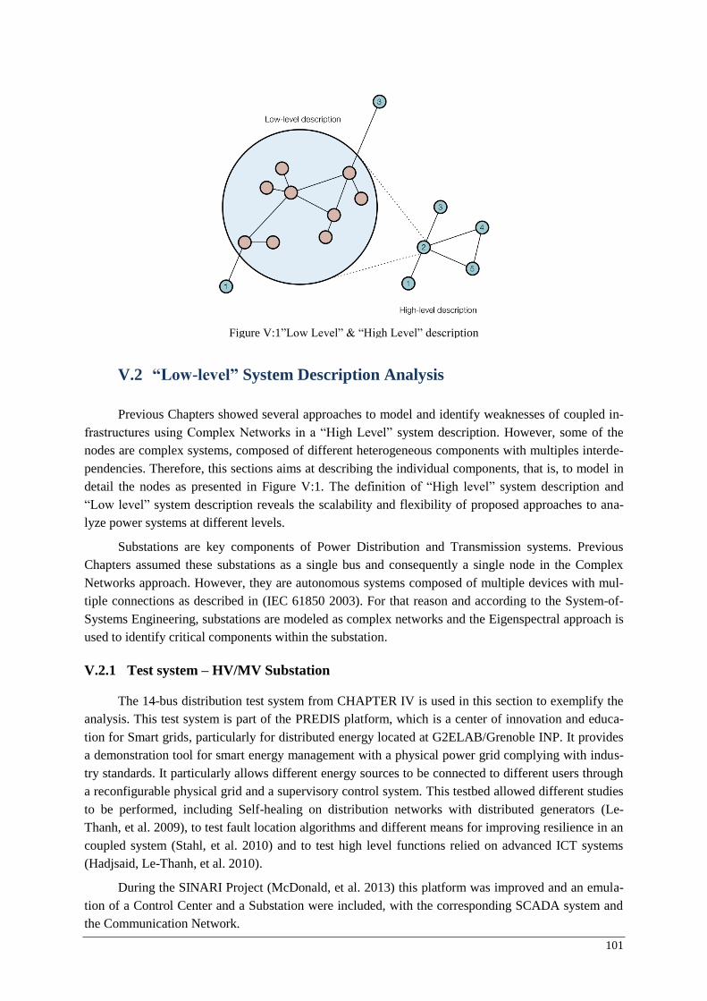
101
V.2 “Low-level” System Description Analysis
Previous Chapters showed several approaches to model and identify weaknesses of coupled in-frastructures using Complex Networks in a “High Level” system description. However, some of the nodes are complex systems, composed of different heterogeneous components with multiples interde-pendencies. Therefore, this sections aims at describing the individual components, that is, to model in detail the nodes as presented in Figure V:1. The definition of “High level” system description and “Low level” system description reveals the scalability and flexibility of proposed approaches to ana-lyze power systems at different levels.
Substations are key components of Power Distribution and Transmission systems. Previous Chapters assumed these substations as a single bus and consequently a single node in the Complex Networks approach. However, they are autonomous systems composed of multiple devices with mul-tiple connections as described in (IEC 61850 2003). For that reason and according to the System-of-Systems Engineering, substations are modeled as complex networks and the Eigenspectral approach is used to identify critical components within the substation.
V.2.1 Test system – HV/MV Substation
The 14-bus distribution test system from CHAPTER IV is used in this section to exemplify the analysis. This test system is part of the PREDIS platform, which is a center of innovation and educa-tion for Smart grids, particularly for distributed energy located at G2ELAB/Grenoble INP. It provides a demonstration tool for smart energy management with a physical power grid complying with indus-try standards. It particularly allows different energy sources to be connected to different users through a reconfigurable physical grid and a supervisory control system. This testbed allowed different studies to be performed, including Self-healing on distribution networks with distributed generators (Le-Thanh, et al. 2009), to test fault location algorithms and different means for improving resilience in an coupled system (Stahl, et al. 2010) and to test high level functions relied on advanced ICT systems (Hadjsaid, Le-Thanh, et al. 2010).
During the SINARI Project (McDonald, et al. 2013) this platform was improved and an emula-tion of a Control Center and a Substation were included, with the corresponding SCADA system and the Communication Network.
Figure V:1”Low Level” & “High Level” description
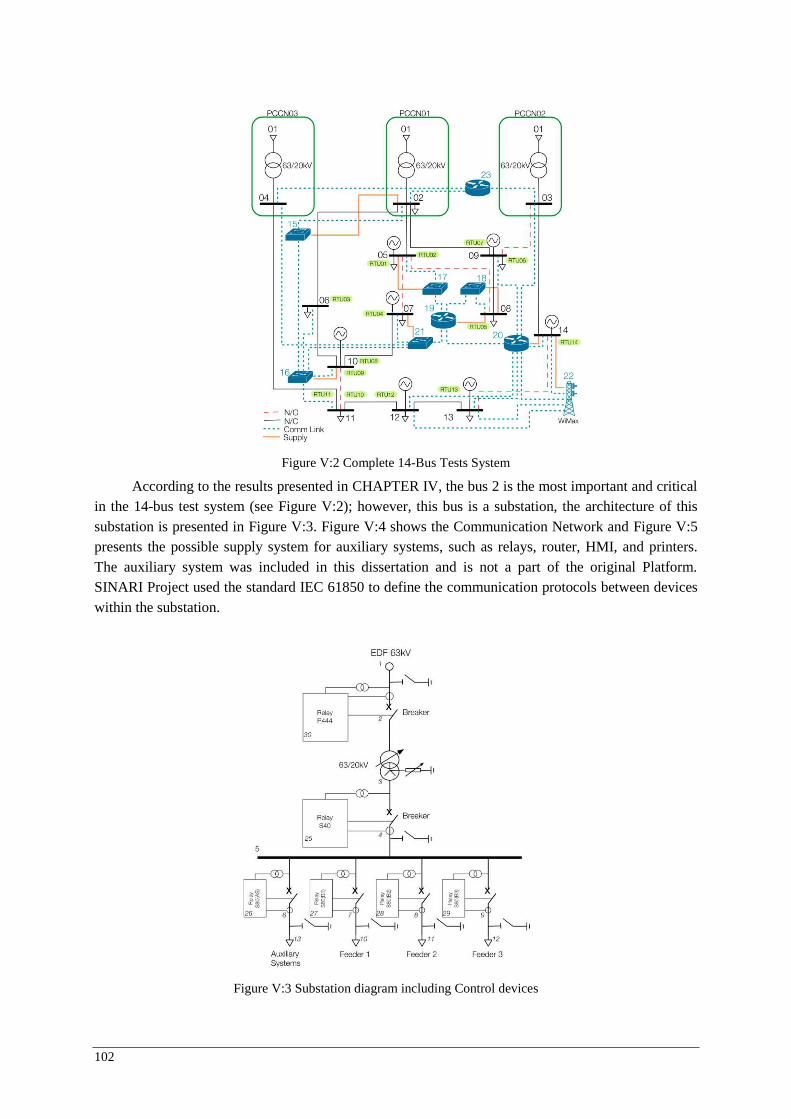
102
According to the results presented in CHAPTER IV, the bus 2 is the most important and critical in the 14-bus test system (see Figure V:2); however, this bus is a substation, the architecture of this substation is presented in Figure V:3. Figure V:4 shows the Communication Network and Figure V:5 presents the possible supply system for auxiliary systems, such as relays, router, HMI, and printers. The auxiliary system was included in this dissertation and is not a part of the original Platform. SINARI Project used the standard IEC 61850 to define the communication protocols between devices within the substation.
Figure V:3 Substation diagram including Control devices
Figure V:2 Complete 14-Bus Tests System
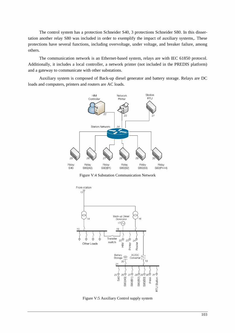
103
The control system has a protection Schneider S40, 3 protections Schneider S80. In this disser-tation another relay S80 was included in order to exemplify the impact of auxiliary systems,. These protections have several functions, including overvoltage, under voltage, and breaker failure, among others.
The communication network is an Ethernet-based system, relays are with IEC 61850 protocol. Additionally, it includes a local controller, a network printer (not included in the PREDIS platform) and a gateway to communicate with other substations.
Auxiliary system is composed of Back-up diesel generator and battery storage. Relays are DC loads and computers, printers and routers are AC loads.
Figure V:4 Substation Communication Network
Figure V:5 Auxiliary Control supply system
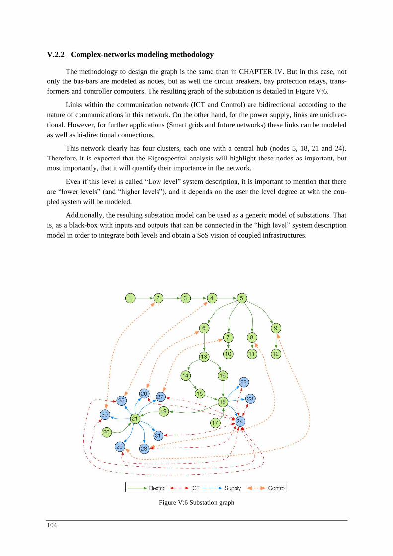
104
V.2.2 Complex-networks modeling methodology
The methodology to design the graph is the same than in CHAPTER IV. But in this case, not only the bus-bars are modeled as nodes, but as well the circuit breakers, bay protection relays, trans-formers and controller computers. The resulting graph of the substation is detailed in Figure V:6.
Links within the communication network (ICT and Control) are bidirectional according to the nature of communications in this network. On the other hand, for the power supply, links are unidirec-tional. However, for further applications (Smart grids and future networks) these links can be modeled as well as bi-directional connections.
This network clearly has four clusters, each one with a central hub (nodes 5, 18, 21 and 24). Therefore, it is expected that the Eigenspectral analysis will highlight these nodes as important, but most importantly, that it will quantify their importance in the network.
Even if this level is called “Low level” system description, it is important to mention that there are “lower levels” (and “higher levels”), and it depends on the user the level degree at with the cou-pled system will be modeled.
Additionally, the resulting substation model can be used as a generic model of substations. That is, as a black-box with inputs and outputs that can be connected in the “high level” system description model in order to integrate both levels and obtain a SoS vision of coupled infrastructures.
Figure V:6 Substation graph
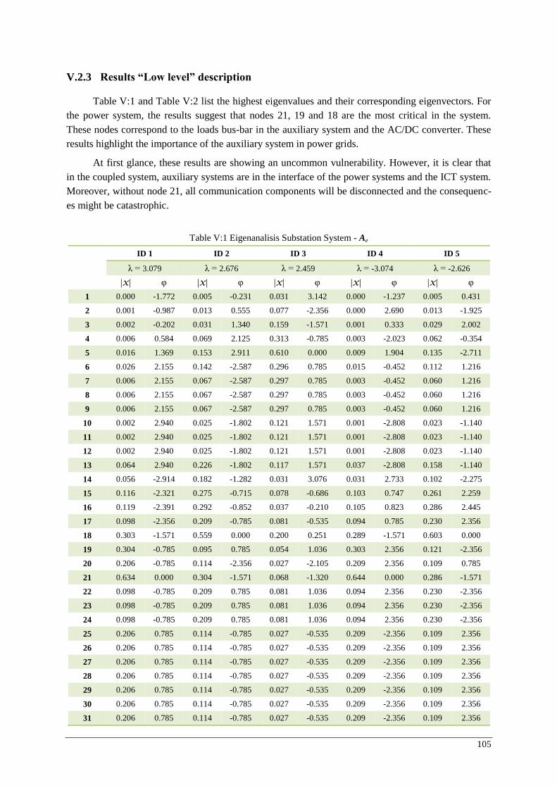
105
V.2.3 Results “Low level” description
Table V:1 and Table V:2 list the highest eigenvalues and their corresponding eigenvectors. For the power system, the results suggest that nodes 21, 19 and 18 are the most critical in the system. These nodes correspond to the loads bus-bar in the auxiliary system and the AC/DC converter. These results highlight the importance of the auxiliary system in power grids.
At first glance, these results are showing an uncommon vulnerability. However, it is clear that in the coupled system, auxiliary systems are in the interface of the power systems and the ICT system. Moreover, without node 21, all communication components will be disconnected and the consequenc-es might be catastrophic.
Table V:1 Eigenanalisis Substation System - Ae
ID 1 ID 2 ID 3 ID 4 ID 5
λ = 3.079 λ = 2.676 λ = 2.459 λ = -3.074 λ = -2.626
|x| φ |x| φ |x| φ |x| φ |x| φ
1 0.000 -1.772 0.005 -0.231 0.031 3.142 0.000 -1.237 0.005 0.431
2 0.001 -0.987 0.013 0.555 0.077 -2.356 0.000 2.690 0.013 -1.925
3 0.002 -0.202 0.031 1.340 0.159 -1.571 0.001 0.333 0.029 2.002
4 0.006 0.584 0.069 2.125 0.313 -0.785 0.003 -2.023 0.062 -0.354
5 0.016 1.369 0.153 2.911 0.610 0.000 0.009 1.904 0.135 -2.711
6 0.026 2.155 0.142 -2.587 0.296 0.785 0.015 -0.452 0.112 1.216
7 0.006 2.155 0.067 -2.587 0.297 0.785 0.003 -0.452 0.060 1.216
8 0.006 2.155 0.067 -2.587 0.297 0.785 0.003 -0.452 0.060 1.216
9 0.006 2.155 0.067 -2.587 0.297 0.785 0.003 -0.452 0.060 1.216
10 0.002 2.940 0.025 -1.802 0.121 1.571 0.001 -2.808 0.023 -1.140
11 0.002 2.940 0.025 -1.802 0.121 1.571 0.001 -2.808 0.023 -1.140
12 0.002 2.940 0.025 -1.802 0.121 1.571 0.001 -2.808 0.023 -1.140
13 0.064 2.940 0.226 -1.802 0.117 1.571 0.037 -2.808 0.158 -1.140
14 0.056 -2.914 0.182 -1.282 0.031 3.076 0.031 2.733 0.102 -2.275
15 0.116 -2.321 0.275 -0.715 0.078 -0.686 0.103 0.747 0.261 2.259
16 0.119 -2.391 0.292 -0.852 0.037 -0.210 0.105 0.823 0.286 2.445
17 0.098 -2.356 0.209 -0.785 0.081 -0.535 0.094 0.785 0.230 2.356
18 0.303 -1.571 0.559 0.000 0.200 0.251 0.289 -1.571 0.603 0.000
19 0.304 -0.785 0.095 0.785 0.054 1.036 0.303 2.356 0.121 -2.356
20 0.206 -0.785 0.114 -2.356 0.027 -2.105 0.209 2.356 0.109 0.785
21 0.634 0.000 0.304 -1.571 0.068 -1.320 0.644 0.000 0.286 -1.571
22 0.098 -0.785 0.209 0.785 0.081 1.036 0.094 2.356 0.230 -2.356
23 0.098 -0.785 0.209 0.785 0.081 1.036 0.094 2.356 0.230 -2.356
24 0.098 -0.785 0.209 0.785 0.081 1.036 0.094 2.356 0.230 -2.356
25 0.206 0.785 0.114 -0.785 0.027 -0.535 0.209 -2.356 0.109 2.356
26 0.206 0.785 0.114 -0.785 0.027 -0.535 0.209 -2.356 0.109 2.356
27 0.206 0.785 0.114 -0.785 0.027 -0.535 0.209 -2.356 0.109 2.356
28 0.206 0.785 0.114 -0.785 0.027 -0.535 0.209 -2.356 0.109 2.356
29 0.206 0.785 0.114 -0.785 0.027 -0.535 0.209 -2.356 0.109 2.356
30 0.206 0.785 0.114 -0.785 0.027 -0.535 0.209 -2.356 0.109 2.356
31 0.206 0.785 0.114 -0.785 0.027 -0.535 0.209 -2.356 0.109 2.356
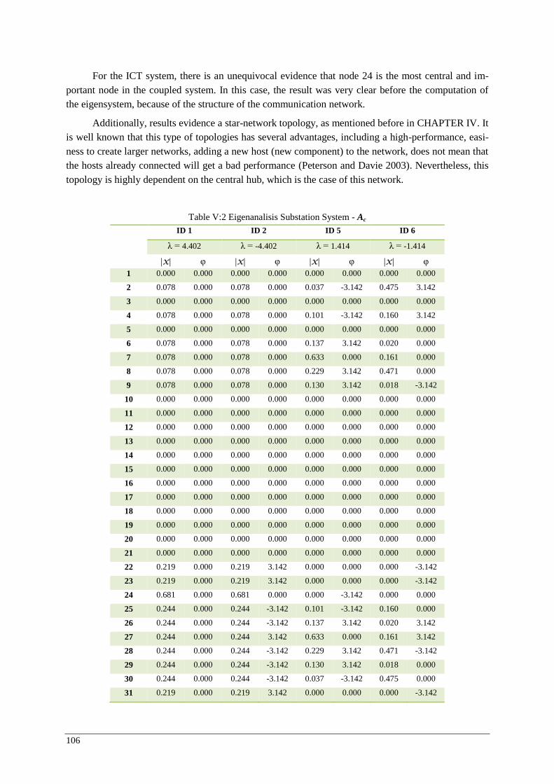
106
For the ICT system, there is an unequivocal evidence that node 24 is the most central and im-portant node in the coupled system. In this case, the result was very clear before the computation of the eigensystem, because of the structure of the communication network.
Additionally, results evidence a star-network topology, as mentioned before in CHAPTER IV. It is well known that this type of topologies has several advantages, including a high-performance, easi-ness to create larger networks, adding a new host (new component) to the network, does not mean that the hosts already connected will get a bad performance (Peterson and Davie 2003). Nevertheless, this topology is highly dependent on the central hub, which is the case of this network.
Table V:2 Eigenanalisis Substation System - Ac
ID 1 ID 2 ID 5 ID 6
λ = 4.402 λ = -4.402 λ = 1.414 λ = -1.414
|x| φ |x| φ |x| φ |x| φ 1 0.000 0.000 0.000 0.000 0.000 0.000 0.000 0.000
2 0.078 0.000 0.078 0.000 0.037 -3.142 0.475 3.142
3 0.000 0.000 0.000 0.000 0.000 0.000 0.000 0.000
4 0.078 0.000 0.078 0.000 0.101 -3.142 0.160 3.142
5 0.000 0.000 0.000 0.000 0.000 0.000 0.000 0.000
6 0.078 0.000 0.078 0.000 0.137 3.142 0.020 0.000
7 0.078 0.000 0.078 0.000 0.633 0.000 0.161 0.000
8 0.078 0.000 0.078 0.000 0.229 3.142 0.471 0.000
9 0.078 0.000 0.078 0.000 0.130 3.142 0.018 -3.142
10 0.000 0.000 0.000 0.000 0.000 0.000 0.000 0.000
11 0.000 0.000 0.000 0.000 0.000 0.000 0.000 0.000
12 0.000 0.000 0.000 0.000 0.000 0.000 0.000 0.000
13 0.000 0.000 0.000 0.000 0.000 0.000 0.000 0.000
14 0.000 0.000 0.000 0.000 0.000 0.000 0.000 0.000
15 0.000 0.000 0.000 0.000 0.000 0.000 0.000 0.000
16 0.000 0.000 0.000 0.000 0.000 0.000 0.000 0.000
17 0.000 0.000 0.000 0.000 0.000 0.000 0.000 0.000
18 0.000 0.000 0.000 0.000 0.000 0.000 0.000 0.000
19 0.000 0.000 0.000 0.000 0.000 0.000 0.000 0.000
20 0.000 0.000 0.000 0.000 0.000 0.000 0.000 0.000
21 0.000 0.000 0.000 0.000 0.000 0.000 0.000 0.000
22 0.219 0.000 0.219 3.142 0.000 0.000 0.000 -3.142
23 0.219 0.000 0.219 3.142 0.000 0.000 0.000 -3.142
24 0.681 0.000 0.681 0.000 0.000 -3.142 0.000 0.000
25 0.244 0.000 0.244 -3.142 0.101 -3.142 0.160 0.000
26 0.244 0.000 0.244 -3.142 0.137 3.142 0.020 3.142
27 0.244 0.000 0.244 3.142 0.633 0.000 0.161 3.142
28 0.244 0.000 0.244 -3.142 0.229 3.142 0.471 -3.142
29 0.244 0.000 0.244 -3.142 0.130 3.142 0.018 0.000
30 0.244 0.000 0.244 -3.142 0.037 -3.142 0.475 0.000
31 0.219 0.000 0.219 3.142 0.000 0.000 0.000 -3.142
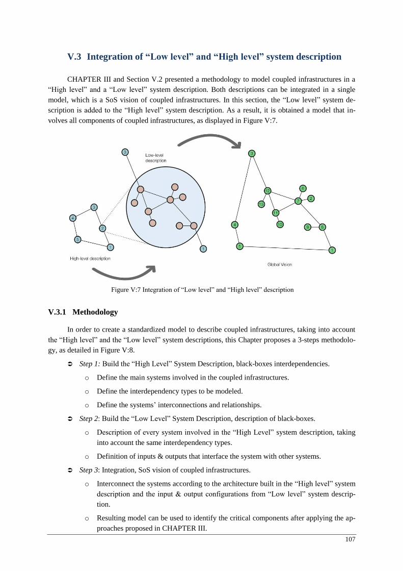
107
V.3 Integration of “Low level” and “High level” system description
CHAPTER III and Section V.2 presented a methodology to model coupled infrastructures in a “High level” and a “Low level” system description. Both descriptions can be integrated in a single model, which is a SoS vision of coupled infrastructures. In this section, the “Low level” system de-scription is added to the “High level” system description. As a result, it is obtained a model that in-volves all components of coupled infrastructures, as displayed in Figure V:7.
V.3.1 Methodology
In order to create a standardized model to describe coupled infrastructures, taking into account the “High level” and the “Low level” system descriptions, this Chapter proposes a 3-steps methodolo-gy, as detailed in Figure V:8.
Step 1: Build the “High Level” System Description, black-boxes interdependencies.
o Define the main systems involved in the coupled infrastructures.
o Define the interdependency types to be modeled.
o Define the systems’ interconnections and relationships.
Step 2: Build the “Low Level” System Description, description of black-boxes.
o Description of every system involved in the “High Level” system description, taking into account the same interdependency types.
o Definition of inputs & outputs that interface the system with other systems.
Step 3: Integration, SoS vision of coupled infrastructures.
o Interconnect the systems according to the architecture built in the “High level” system description and the input & output configurations from “Low level” system descrip-tion.
o Resulting model can be used to identify the critical components after applying the ap-proaches proposed in CHAPTER III.
Figure V:7 Integration of “Low level” and “High level” description
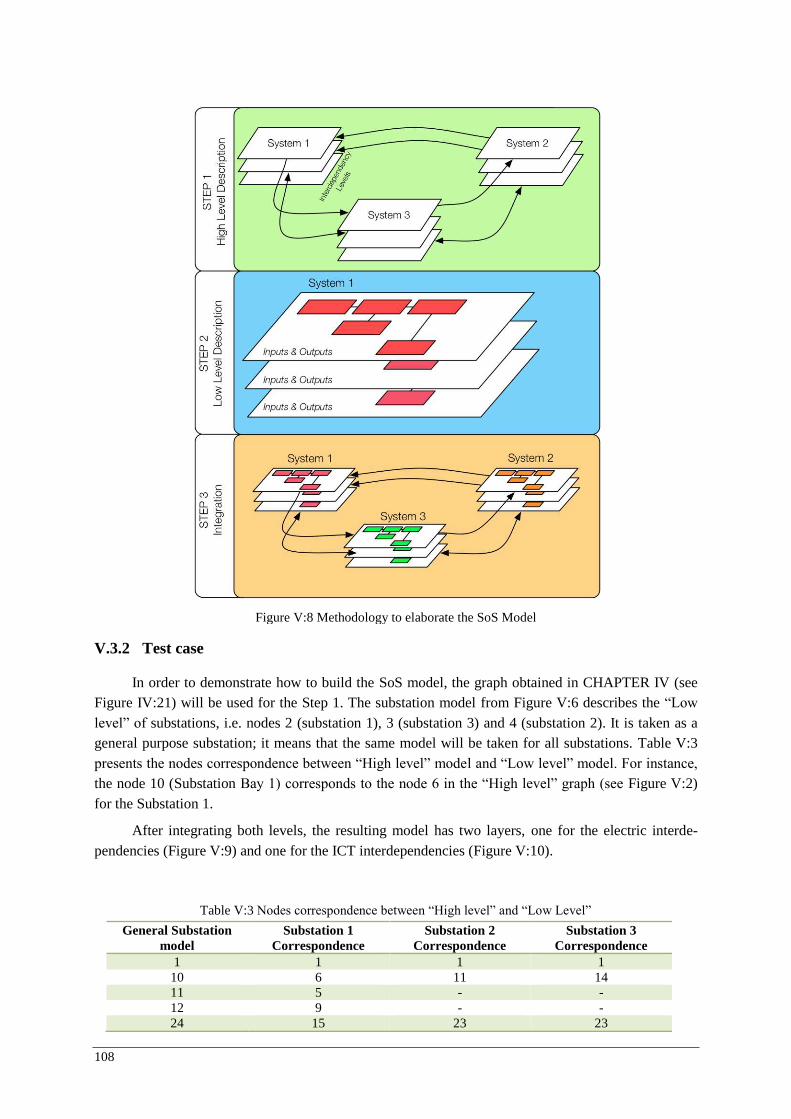
108
V.3.2 Test case
In order to demonstrate how to build the SoS model, the graph obtained in CHAPTER IV (see Figure IV:21) will be used for the Step 1. The substation model from Figure V:6 describes the “Low level” of substations, i.e. nodes 2 (substation 1), 3 (substation 3) and 4 (substation 2). It is taken as a general purpose substation; it means that the same model will be taken for all substations. Table V:3 presents the nodes correspondence between “High level” model and “Low level” model. For instance, the node 10 (Substation Bay 1) corresponds to the node 6 in the “High level” graph (see Figure V:2) for the Substation 1.
After integrating both levels, the resulting model has two layers, one for the electric interde-pendencies (Figure V:9) and one for the ICT interdependencies (Figure V:10).
Figure V:8 Methodology to elaborate the SoS Model
Table V:3 Nodes correspondence between “High level” and “Low Level”
General Substation model
Substation 1 Correspondence
Substation 2 Correspondence
Substation 3 Correspondence
1 1 1 1 10 6 11 14 11 5 - - 12 9 - - 24 15 23 23
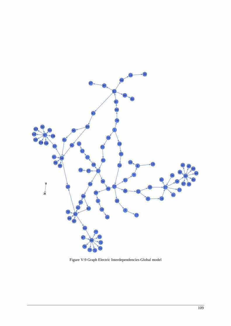
109
Figure V:9 Graph Electric Interdependencies Global model
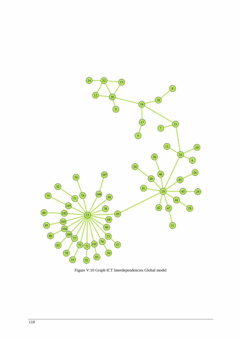
110
Figure V:10 Graph ICT Interdependencies Global model
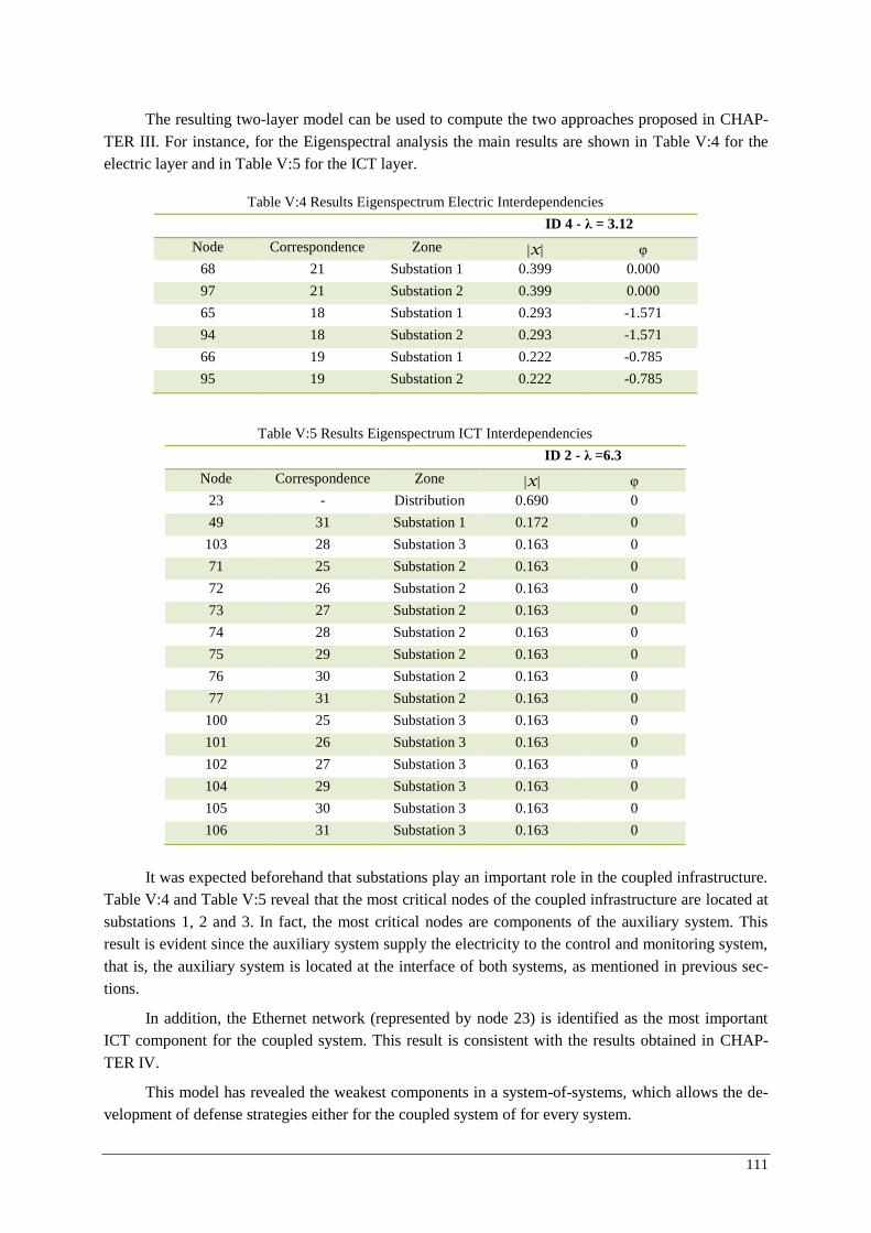
111
The resulting two-layer model can be used to compute the two approaches proposed in CHAP-TER III. For instance, for the Eigenspectral analysis the main results are shown in Table V:4 for the electric layer and in Table V:5 for the ICT layer.
It was expected beforehand that substations play an important role in the coupled infrastructure. Table V:4 and Table V:5 reveal that the most critical nodes of the coupled infrastructure are located at substations 1, 2 and 3. In fact, the most critical nodes are components of the auxiliary system. This result is evident since the auxiliary system supply the electricity to the control and monitoring system, that is, the auxiliary system is located at the interface of both systems, as mentioned in previous sec-tions.
In addition, the Ethernet network (represented by node 23) is identified as the most important ICT component for the coupled system. This result is consistent with the results obtained in CHAP-TER IV.
This model has revealed the weakest components in a system-of-systems, which allows the de-velopment of defense strategies either for the coupled system of for every system.
Table V:4 Results Eigenspectrum Electric Interdependencies
ID 4 - λ = 3.12
Node Correspondence Zone |x| φ 68 21 Substation 1 0.399 0.000
97 21 Substation 2 0.399 0.000
65 18 Substation 1 0.293 -1.571
94 18 Substation 2 0.293 -1.571
66 19 Substation 1 0.222 -0.785
95 19 Substation 2 0.222 -0.785
Table V:5 Results Eigenspectrum ICT Interdependencies
ID 2 - λ =6.3
Node Correspondence Zone |x| φ 23 - Distribution 0.690 0
49 31 Substation 1 0.172 0
103 28 Substation 3 0.163 0
71 25 Substation 2 0.163 0
72 26 Substation 2 0.163 0
73 27 Substation 2 0.163 0
74 28 Substation 2 0.163 0
75 29 Substation 2 0.163 0
76 30 Substation 2 0.163 0
77 31 Substation 2 0.163 0
100 25 Substation 3 0.163 0
101 26 Substation 3 0.163 0
102 27 Substation 3 0.163 0
104 29 Substation 3 0.163 0
105 30 Substation 3 0.163 0
106 31 Substation 3 0.163 0

112
V.4 Smart-Grids: A SGAM-based System-of-Systems vision
One of the objectives of this dissertation is to explore the feasibility of using the proposed ap-proaches at different levels, according to the most recent architectures proposed for Smart Grids. Pre-vious Chapters and sections proposed different methods (or a vision) to model coupled infrastructures, from a “high level description” and from a “low level description.” This Section aims at describing the Smart Grids Architecture model (SGAM) and proposes a general methodology to model Smart Grids’ interdependencies.
In order to better understand the SGAM, it is important to define a Smart Grid. According to the European Commission “a Smart grid is an electricity network that can integrate in a cost efficient manner the behavior and actions of all users connected to it - generators, consumers and those that do
both - in order to ensure economically efficient, sustainable power system with low losses and high levels of quality and security of supply and safety” (EU Commission Task Force for Smart Grids 2010)
However, even if there is an official definition of Smart Grid, apparently each enterprise and re-search center is developing its own Smart Grid model and definition. There are some researchers that call it the “Smarter Grid,” signaling that current grids are smart as well, but in a lower level (ABB Inc 2009).
Therefore, in order to fulfill the tasks of mandate M/490 (see Appendix C) and to create a con-sensus on Smart Grids Architectures, the SGAM was created (CEN-CENELEC-ETSI 2012).
V.4.1 Smart Grid Architecture Model (SGAM)
(CEN-CENELEC-ETSI 2012) identified three major problems in the development of Smart Grids today.
How to compare the different Smart Grids Architectures proposed?
How to choose a Smart Grid Standard? Taking into account that there are several standards
Figure V:11 SGAM Framework (CEN-CENELEC-ETSI 2012)

113
with many limitations, gaps and overlaps.
How to migrate to Smart Grid from an architectural point of view?
According to them, a Smart Grid is a “complex system of systems for which a common under-standing of its major building and how they interrelate must be broadly shared.” For that reason, in order to create a standardized architecture model, three main aspects were evaluated: domains, zones and interoperability layers. These aspects are described in next subsections.
V.4.1.1 SGAM: Domains
“Domains” describe the energy conversion chain, that is, a description of main actors in the Smart grid. These domains were selected according to the NIST Smart Grid Standard (NIST 2012). Additionally, the DER (Distributed Energy Resources) Domain was included. Therefore, the main domains of Smart Grids are:
Generation: The bulk generation, e.g. fossil, nuclear, large scale solar power plants, hydro power plants and off-shore wind farms.
Transmission: The infrastructure that transports electricity over long distances.
Distribution: The infrastructure that distributes electricity to customers.
DER: Small-scale power generation, from 3kW to 10MW.
Customer: End-users (consumers), but they have the possibility to produce electricity, i.e. prosumers.
V.4.1.2 SGAM: Zones
“Smart Grids” are divided into six zones:
Process: This zone includes all types of energy transformation, e.g. physical, chemical or spatial. In addition, it includes the physical equipment.
Field: It contains all the equipment used to control, protect and monitor the processes within the Smart Grid.
Station: This zone includes the aggregators of all fields’ equipment.
Operation: It hosts the power system control operation, including DMS, EMS, and others.
Enterprise: It covers all the commercial and organizational processes, services and infra-structures for enterprises.
Market: It reflects the market operations possible in the energy conversion chain.
V.4.1.3 SGAM: Interoperability Layers
The interoperability layers cover the different interdependencies between domains in many zones. This is very close to the vision proposed in CHAPTER 3 (see Figure III :23 and Figure III :24). SGAM proposes five layers:
Component: It represents the physical layer, including all participating components in the Smart Grids. For instance, power systems equipment, protection/control devices or network infrastructure.
Function: It describes the functions and services including their relationships.
114
Information: It contains all the information that is used and exchanged between functions, services and components.
Communication: It describes the protocols and mechanisms used to exchange the infor-mation.
Business: It represents all business capabilities and processes to support business executives in decision making processes.
V.4.1.4 SGAM: Architecture
The resulting architecture that puts all the domains, zones and layers together is detailed in Fi-gure V:11. This representation enables the understanding of the relationships in the Smart Grid. In addition, this architecture can be used to describe the interoperability between two (or more) systems, taking into account the component, communication, information, function and business layers, which are called the “cross-cutting issues.”
V.4.2 Complex Networks modeling
This section proposes a standardized methodology in order to model Smart Grids, based in the Smart Grid Reference Architecture and the integration of “High level” and “Low level” descriptions.
Following the methodology detailed in Figure V:8, the three steps are described in the following subsections.
V.4.2.1 Step 1: High level system Description
Define the main systems involved in the coupled infrastructures.
At this step, 8 systems are identified: Markets, Operations, Service provider, Transmission net-work, Distribution Network, Customer, Bulk generation and Distributed Energy Resources.
Define the interdependency types to be modeled.
Considering the interdependencies types presented in Section I.2.2 (physical, cyber, geographic and logical) and taking into account the interoperability layers, four interdependency levels were de-fined: physical level is composed of electrical interdependencies between components of SGAM Component level. Cyber level is composed of communication interdependencies between components at the SGAM Component level. This layer can be supported as well by the Information layer. Geo-graphic level according to the zones proposed in the SGAM framework. Logical level composed of function relationships, from the function layer in the SGAM framework.
Define the systems interconnections and relationships.
The NIST model (NIST 2012) and the SGAM Reference architecture (CEN-CENELEC-ETSI 2012) presented the interconnections between the actors (or domains) in the Smart Grid. Figure V:12 presents the interconnections between these domains and their interdependency levels. Dotted lines were added in order to take into account the electrical dependency of markets, operation and service provider.
V.4.2.2 Step 2: Low Level system Description
Description of every system involved in the “High Level” description, taking into account the same interdependency levels.
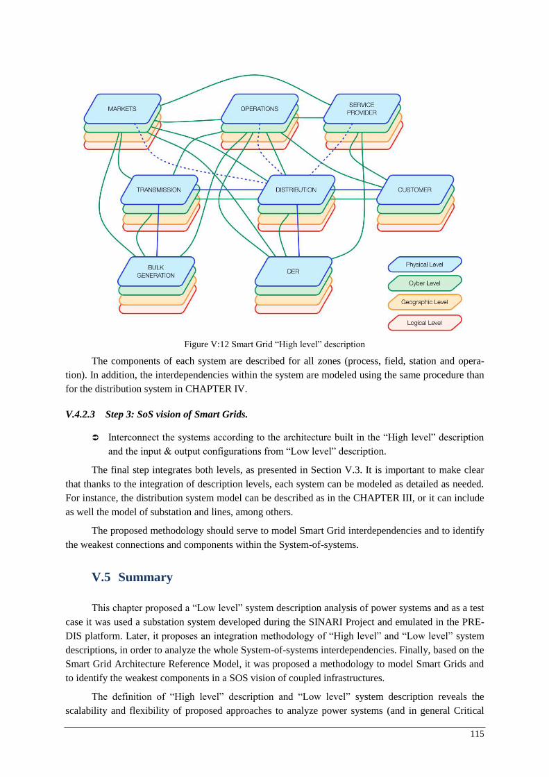
115
The components of each system are described for all zones (process, field, station and opera-tion). In addition, the interdependencies within the system are modeled using the same procedure than for the distribution system in CHAPTER IV.
V.4.2.3 Step 3: SoS vision of Smart Grids.
Interconnect the systems according to the architecture built in the “High level” description and the input & output configurations from “Low level” description.
The final step integrates both levels, as presented in Section V.3. It is important to make clear that thanks to the integration of description levels, each system can be modeled as detailed as needed. For instance, the distribution system model can be described as in the CHAPTER III, or it can include as well the model of substation and lines, among others.
The proposed methodology should serve to model Smart Grid interdependencies and to identify the weakest connections and components within the System-of-systems.
V.5 Summary
This chapter proposed a “Low level” system description analysis of power systems and as a test case it was used a substation system developed during the SINARI Project and emulated in the PRE-DIS platform. Later, it proposes an integration methodology of “High level” and “Low level” system descriptions, in order to analyze the whole System-of-systems interdependencies. Finally, based on the Smart Grid Architecture Reference Model, it was proposed a methodology to model Smart Grids and to identify the weakest components in a SOS vision of coupled infrastructures.
The definition of “High level” description and “Low level” system description reveals the scalability and flexibility of proposed approaches to analyze power systems (and in general Critical
Figure V:12 Smart Grid “High level” description

116
infrastructures) at different levels taking into account multiple interdependencies.
The main result of this Chapter is a methodology that aims at identifying the vulnerabilities and interdependencies of power systems facing the wide deployment of Information and Communication technologies, including substations and distributed energy resources.
117
GENERAL CONCLUSIONS
There is no real ending. It’s just the place where you stop the story.
Frank Herbert
Power Distribution Systems demand a continuous research to ensure high levels of reliability, availability and security. As a consequence, new equipment has been created to support the supervi-sion, control and protection of Power Distribution Systems. This new equipment relies on fast, secure and efficient communication networks.
However, last years have been marked by high deployment of Information and Telecommunica-tion Technologies on many infrastructures, making a whole complex network of coupled heterogene-ous infrastructures, creating a huge System-of-Systems.
As well, power systems face other challenges, such as the beginning of a liberalized marked and the insertion of decentralized generation. Yet these two challenges highly rely on ICT networks.
Generally speaking, ICT deployment has been very positive and has improved the supervision and control, supported the operation decision making process, policy making and markets regulation. Nevertheless, recent events have shown that there are new vulnerabilities that emerge from the interac-tions and interplays among Critical infrastructures, e.g. Stuxnet worm, Ohio Davis-Besse nuclear plant attack or the 2003 US – Canada Blackout.
This dissertation described some of the main interplays and interdependencies among critical in-frastructures. Particularly, it investigated and described the interdependencies among power distribu-tion networks, information and communication infrastructure and the different control and supervision hierarchical levels, to better understand the studied problem.
Among the multiple interdependencies between infrastructures, this dissertation explored those that are capable of creating cascading effects from one infrastructure to the other.
In this context, the US Homeland Security Department and the European Commission have ad-dressed this problem, and new policies are being created in order to ensure the continuity of service of Critical Infrastructures. As well, many projects have been developed in order to understand these complex interactions, one of them: the SINARI Project, sponsored by the ANR-France. This thesis was developed as part of this project.
This context opened a new research direction with new challenges and goals. One of them is the
118
need of new tools and methods to understand, to identify and to quantify the interdependencies and vulnerabilities that can emerge from the interconnection of critical infrastructures from micro and macro visions. The study of several methods to model critical infrastructures show the many aspects covered by researchers around the world to understand complex systems.
This dissertation reviews many popular methods, including Agent-Based models, Bayesian Networks, Boolean Logic driven Bayesian Networks, Combined Simulators, Petri Networks and Complex Networks. However, these methods have unlike objectives, making impossible to compare their results. Instead, a sum of these methods can help to understand the dynamics on critical infra-structures, to design adequate protections and to plan adequate emergency actions against attacks and failures.
Among these methods, Complex Networks showed that they are capable and suitable to model and to reflect the topological properties of large complex systems. This dissertation is based on the idea that Power Systems are one of the most complex modern networks and there is little understand-ing of their structure and properties. Thus, to understand this complex system it is needed to map out its interactions and interdependencies in a network-based model.
Two “High-level” models (or macro-vision models) were proposed, these models aim at de-scribing the asymmetrical communication patterns that can be found in heterogeneous infrastructures. In order to create these models, the classic theory of complex networks was modified and a new math-ematical dimension was introduced in the characteristic adjacency matrix. As well, this adjacency matrix was transported to the Hilbert Space using Hermitian Matrices to obtain the Eigen-system that characterizes the interdependent infrastructures.
The significance and originality of this dissertation lays in its ability to bridge two infrastruc-tures in a single model, conserving their own characteristics and highlighting the interconnections among them. As well, because of the flexibility and scalability of the model, it is not limited to the type of infrastructure to model; moreover n-infrastructures can be studied in a multi-dimensional mod-el.
Therefore, the proposed methods tailor the complex networks to the study of critical infrastruc-tures vulnerabilities, developing a networks-based representation of the interacting infrastructures that allows treating the interdependencies problem in a more unified fashion.
Throughout the course of this dissertation many difficulties (or challenges) were found, includ-ing the little understanding of power distribution systems, information and communication networks and control systems working as a whole coupled system. Since each infrastructure represents a large complex domain, it is complicated to assemble a set of definitions, procedures and component of het-erogeneous systems. But at the same time, this notoriously difficult problem highlights the novelty of this dissertation, because it shows a slight headway in the field of modeling of interdependent infra-structures. Another major difficulty was the lack of data and tools to validate the models.
The main disadvantage of the presented approaches is that they are purely topological. Howev-er, this study can be considered as the foundation of further work dealing with vulnerability studies of interdependent infrastructures. As well, some indexes reflect somehow the flow of data and electricity within the networks, e.g. Betweenness Centrality and Efficiency metrics.
A “Low level” (or micro-vision) model is proposed to identify the vulnerabilities in a deeper level. This model was integrated with the “High level” model in order to have a complete analysis of coupled infrastructures and as result of this integration, a 3-steps methodology was obtained to analyze coupled infrastructures at different description levels.
119
Finally, this dissertation proposed a methodology to model Smart Grids, based in the Smart Grid Architecture Model (SGAM). This methodology exploits the “High level” and “Low level” sys-tem description in order to create a model that considers all the domains, zones and interdependencies between components in a Smart Grid. However, it is clear than on a complex system like a Smart Grid, it is not possible to consider all aspects that define their interdependencies. Although it is true, the proposed methodology should serve as a first step to identify weaknesses in Smart Grids and should inspire future work.
Therefore, further work should be focused on dynamic networks that will represent the dynam-ical behavior of infrastructures. However, it is a very complex endeavor and since deeper investiga-tions lead to more questions, further work has to be realized by a multi-disciplinary team including not only electrical and systems engineers, but also mathematicians, sociologists and economist in order to represent the real behavior of coupled heterogeneous infrastructures.
Some of the proposed research challenges include:
Continue the modeling of coupled infrastructures using Complex-weighted complex networks. As it was mention, the proposed approaches are a first step to model multi-dimensional interdependencies between critical infrastructures. This work could be extend-ed in order to consider many other infrastructures’ interdependencies. Then, it is possible to integrate cross disciplinary interdependencies. For instance, gas and water transport interde-pendencies with the generation units in the “Low level” description.
Smart Grids modeling. Last Chapter proposed a methodology to model Smart Grids and to identify weaknesses that emerge from the integration of multiple components located at dif-ferent domains and zones. This methodology should serve to compare different architec-tures and to identify potential vulnerabilities.
Develop (reinforce) self-healing algorithms using complex networks. Thanks to the scalability and flexibility of proposed approaches. They can be used to evaluate optimal configuration after a failure, from a topological viewpoint. It could either reduce the number of options (new architectures) or propose new architectures that might not be evident using other methods.
Create a test case of interdependent critical infrastructures. One of the main limitations during this research was the lack of complete test cases. Therefore, an important and critical research line is the development of test cases in order to validate new methods and models that include coupled infrastructures. Some of this research is already being developed at G2ELAB.
Development of failure detection/prediction algorithms. Since topology-driven analysis reveals several weaknesses of coupled infrastructures, this analysis can be used to reinforce or to develop new failure detection/prediction algorithms.
System-of-Systems Engineering & Global vision of Systems. As a short-term research line, many “Low-level” general purpose models can be created in order to identify optimal architectures. For instance, create black-boxes for all types of substation configuration that can be easily included in the “High-level” model.
Multiple infrastructure planning : It includes the development of tools to address multiple heterogeneous infrastructures in the planning process.

121
RÉSUMÉ EN FRANÇAIS
If you don't have time to do it right,
when will you have time to do it over?
John Wooden
SOMMAIRE
1. INTRODUCTION GENERALE ................................................................................................. 122
2. VERROUS SCIENTIFIQUES .................................................................................................... 124
2.1. INTERDEPENDANCES CYBER-PHYSIQUES .................................................................... 124
2.2. MANQUE DES METHODES DE MODELISATION .............................................................. 124
2.3. INFRASTRUCTURES HETEROGENES .............................................................................. 127
3. PROJET SINARI ................................................................................................................... 127
4. OBJECTIFS DE LA THESE ...................................................................................................... 127
5. LA SOLUTION PROPOSEE ..................................................................................................... 128
6. METHODOLOGIE .................................................................................................................. 128
6.1. CONCEPTS DE BASE DES RESEAUX COMPLEXES ......................................................... 129
6.2. APPROCHE TOPOLOGIQUE ........................................................................................... 132
6.2.1. Degré des Nœuds ............................................................................................ 133
6.2.2. Betweenness Centrality ................................................................................... 133
6.2.3. L’efficacité ...................................................................................................... 134
6.2.4. Système de Test .............................................................................................. 135
6.2.1. Les résultats principaux .................................................................................. 138
6.3. L’APPROCHE SPECTRALE ............................................................................................. 142
6.3.1. Le degré complexe des Nœuds ....................................................................... 142
6.3.2. La centralité spectrale ..................................................................................... 143
6.3.3. Les résultats principaux .................................................................................. 143
6.4. DESCRIPTION « LOW LEVEL » ....................................................................................... 146
6.5. VISION GLOBALE DU SYSTEME .................................................................................... 149
7. CONCLUSIONS ET PERSPECTIVES ......................................................................................... 150
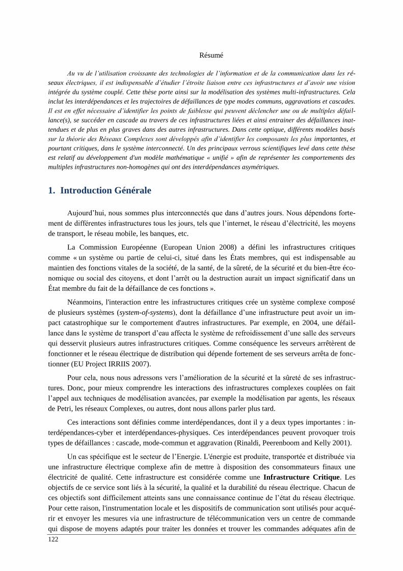
122
Résumé
Au vu de l’utilisation croissante des technologies de l’information et de la communication dans les ré-
seaux électriques, il est indispensable d’étudier l’étroite liaison entre ces infrastructures et d’avoir une vision intégrée du système couplé. Cette thèse porte ainsi sur la modélisation des systèmes multi-infrastructures. Cela
inclut les interdépendances et les trajectoires de défaillances de type modes communs, aggravations et cascades.
Il est en effet nécessaire d’identifier les points de faiblesse qui peuvent déclencher une ou de multiples défail-lance(s), se succéder en cascade au travers de ces infrastructures liées et ainsi entrainer des défaillances inat-
tendues et de plus en plus graves dans des autres infrastructures. Dans cette optique, différents modèles basés
sur la théorie des Réseaux Complexes sont développés afin d’identifier les composants les plus importantes, et
pourtant critiques, dans le système interconnecté. Un des principaux verrous scientifiques levé dans cette thèse
est relatif au développement d'un modèle mathématique « unifié » afin de représenter les comportements des
multiples infrastructures non-homogènes qui ont des interdépendances asymétriques.
1. Introduction Générale
Aujourd’hui, nous sommes plus interconnectés que dans d’autres jours. Nous dépendons forte-ment de différentes infrastructures tous les jours, tels que l’internet, le réseau d’électricité, les moyens de transport, le réseau mobile, les banques, etc.
La Commission Européenne (European Union 2008) a défini les infrastructures critiques comme « un système ou partie de celui-ci, situé dans les États membres, qui est indispensable au maintien des fonctions vitales de la société, de la santé, de la sûreté, de la sécurité et du bien-être éco-nomique ou social des citoyens, et dont l’arrêt ou la destruction aurait un impact significatif dans un État membre du fait de la défaillance de ces fonctions ».
Néanmoins, l'interaction entre les infrastructures critiques crée un système complexe composé de plusieurs systèmes (system-of-systems), dont la défaillance d’une infrastructure peut avoir un im-pact catastrophique sur le comportement d'autres infrastructures. Par exemple, en 2004, une défail-lance dans le système de transport d’eau affecta le système de refroidissement d’une salle des serveurs qui desservit plusieurs autres infrastructures critiques. Comme conséquence les serveurs arrêtèrent de fonctionner et le réseau électrique de distribution qui dépende fortement de ses serveurs arrêta de fonc-tionner (EU Project IRRIIS 2007).
Pour cela, nous nous adressons vers l’amélioration de la sécurité et la sûreté de ses infrastruc-tures. Donc, pour mieux comprendre les interactions des infrastructures complexes couplées on fait l’appel aux techniques de modélisation avancées, par exemple la modélisation par agents, les réseaux de Petri, les réseaux Complexes, ou autres, dont nous allons parler plus tard.
Ces interactions sont définies comme interdépendances, dont il y a deux types importantes : in-terdépendances-cyber et interdépendances-physiques. Ces interdépendances peuvent provoquer trois types de défaillances : cascade, mode-commun et aggravation (Rinaldi, Peerenboom and Kelly 2001).
Un cas spécifique est le secteur de l’Energie. L'énergie est produite, transportée et distribuée via une infrastructure électrique complexe afin de mettre à disposition des consommateurs finaux une électricité de qualité. Cette infrastructure est considérée comme une Infrastructure Critique . Les objectifs de ce service sont liés à la sécurité, la qualité et la durabilité du réseau électrique. Chacun de ces objectifs sont difficilement atteints sans une connaissance continue de l’état du réseau électrique. Pour cette raison, l'instrumentation locale et les dispositifs de communication sont utilisés pour acqué-rir et envoyer les mesures via une infrastructure de télécommunication vers un centre de commande qui dispose de moyens adaptés pour traiter les données et trouver les commandes adéquates afin de
123
maintenir les paramètres électriques dans des valeurs acceptables, c’est-à-dire, de piloter le réseau correctement et d’assurer l’exploitation.
Les Technologies de l’Information et de la Communication (TIC) sont complexes, car ces dis-positifs sont, entre autres, très hétérogènes et fortement interconnectés avec autres systèmes tels que les systèmes de contrôle et le réseau de capteurs du système. Malgré toutes les mesures de sécurité, il y a un fort impact des systèmes TIC sur la performance des Réseaux Electriques. Par exemple, le Mid-west et le Nord-Ouest des Etats-Unis et de l’Ontario au Canada ont subi une des pannes les plus catas-trophiques de l'histoire en 2003, causée par la défaillance dans plusieurs lignes électriques et par l’ignorance des opérateurs des centres de contrôle qui ne les voyaient parce que le système d'alarme était en panne minutes avant la panne électrique. Cela a provoqué un phénomène de cascade qui a coûté entre US $ 7 et 10 milliards, et affecté près de 50 millions de citoyens. Autres exemples sont cités dans l’Appendice A. En effet, selon l'ICS-CERT le secteur de l'énergie a subi 41,4% des cyberat-taques contre des infrastructures critiques en 2012 (voir Figure F - 1).
Ce problème a été déjà abordé par le Département Américain de la Sécurité Intérieure et par la Commission Européenne. Comme résultat, de nouvelles politiques sont en cours de rédaction afin d'assurer la continuité de service des infrastructures critiques. De même que de nombreux projets ont été développées afin de comprendre ces interactions. Le projet SINARI est l’un d’entre eux, financé par l'ANR - France. Cette thèse a été réalisée dans le cadre de ce projet.
Ce chapitre de résumé est divisé en 7 sections très succinctes.
Section 2 : Porte sur les principaux verrous scientifiques et défis.
Section 3 : Décrit les objectifs du projet SINARI dont cette thèse a fait partie.
Section 4 : L’objectif de la thèse. Section 5 : Présentation de la solution proposée.
Section 6 : Développement de la méthodologie et présentation de quelques résultats.
Section 7 : Conclusions et perspectives.
Cette division a été inspirée par les transparents présentés lors de la soutenance qui eut lieu le 23 Octobre 2013.
Figure F - 1 Incidents par Secteur – 198 Total Année Fiscale 2012 (ICS-CERT 2012)
Energie 41,4%
Dams 0,5%
Critical Manuf 4,0%
Communications 2,0%
Commercial 9,6%
Chemique 3,5%
Banques et Finance 0,5%
Eau 14,6%
Internet 10,6%
Transportation 2,5%
Nuclear 3,0%
IT 0,5% Santé
2,5%
Government 3,5%
Aliments1,0%
124
2. Verrous Scientifiques
Trois verrous scientifiques ont été identifiés : i) Les fortes interdépendances entre composants électriques physiques et les systèmes dites « Cyber ». ii) La manque de méthodes pour comprendre ces interactions complexes. iii) La hétérogénéité des systèmes.
2.1. Interdépendances Cyber-physiques
L’utilisation de plus en plus croissante des systèmes TIC dans les réseaux de distribution peut être responsable des défaillances de type cascade, de mode commun et d’aggravation.
Cette dépendance accrue, malgré les aspects bénéfiques indéniables qu’elle apporte à la con-duite du système, ne va pas sans poser de nouveaux problèmes. Ainsi, face à un mauvais fonctionne-ment d’un composant de l’infrastructure d’information et de communication dans un système de su-pervision, les opérateurs peuvent prendre des décisions non appropriées et affecter sévèrement le sys-tème supervisé. Du même qu’une défaillance dans le réseau électrique peut impacter le fonctionne-ment de l’infrastructure d’information et de la communication, si les mesures de sécurité ne sont pas prévus.
2.2. Manque des méthodes de modélisation
Il est alors nécessaire de pouvoir caractériser les systèmes critiques afin de faciliter l’analyse de risques et la définition de méthodes et de mécanismes locaux et globaux de sécurisation et de fiabilisa-tion efficaces. En effet, la sécurisation des infrastructures critiques est une tâche complexe qui ne peut être atteinte seulement si le comportement des systèmes multi-infrastructures est bien compris et en particulier leurs trajectoires de défaillances et leurs interdépendances de type commun, aggravation et cascade. Cette compréhension peut être atteinte par une modélisation mathématique des différents phénomènes et processus mis en jeu. Ainsi la modélisation des interdépendances entre les infrastruc-tures critiques est une première étape importante en vue de leur sécurisation.
Bien que plusieurs chercheurs aient étudié la vulnérabilité des systèmes électriques et des infras-tructures des TIC, ces études sont encore à un stade embryonnaire et de nombreuses questions restent sans réponse. Par exemple, l’absence de méthodes pour comprendre les interdépendances entre les infrastructures critiques. Une autre difficulté apparaît pour ces modélisations, il s’agit du comporte-ment des êtres humains qui interagissent avec les infrastructures, comportement que l’on peut considé-rer comme relativement imprévisible. En effet, les infrastructures étudiées fonctionnent bien actuelle-ment avec une durée de non fonctionnement très faible par rapport au temps de fonctionnement nor-mal.
Diverses méthodes ont été utilisées pour modéliser les interdépendances des Systèmes TIC et les réseaux électriques. Parmi eux les réseaux de Petri, les réseaux complexes, le cosimulateur et l’utilisation des BDMP (Boolean logic Driven Markov).
La modélisation des infrastructures critiques es une étape essentielle pour identifier les modes de défaillance les plus problématiques et choisir les parades les plus appropriées pour en assurer leur bon fonctionnement. Différentes méthodes sont résumées à continuation :
125
Modélisation par Agents :
(Schläpfer, Kessler et Kröger 2008) ont proposé le « Object-Oriented Hybrid Modeling Ap-proach » et (Panzeri, Setola et Ulivi 2004) ont travaillé sur le « Agent-based input-output
interdependency model ».
Cette approche possède différents avantages par rapport aux techniques de modélisations classiques comme montré dans par (Barton, 2000 et Macal, 2005). Tout d’abord, il n’y a pas besoin de concevoir un modèle de haut niveau pour décrire le comportement complexe d’une infrastructure. À la place, on part du comportement relativement simple de différents composants de bas niveau et on les laisse coopérer. Le comportement émergeant complexe de haut niveau apparaît alors de lui même. De plus, le modèle est modulaire, dont chaque agent intègre sa propre modélisation (algorithme complexe, chaînes de Markov, ou autres), qui peut donc être différente pour chaque composant élémentaire d’un même environnement.
Un autre avantage réside dans son approche intrinsèquement distribuée, ce qui facilite la répartition du calcul sur plusieurs processeurs, si le besoin s’en fait sentir lors de la simulation. Néanmoins, les méthodes mises en œuvre dans les systèmes multi-agents sont parfois assez complexes et constituent souvent un frein à la modélisation des grands systèmes complexes.
Réseaux de Petri :
Les réseaux de Petri peuvent modéliser des systèmes complexes en regroupant plusieurs aspects (aspect fonctionnel, menaces et contremesures (Xu et al., 2006)) composants (homogènes ou hétéro-gènes), ainsi que des évènements discrets (par exemple les alertes) et des évènements continus (par exemple, le flux de données). Les réseaux de Petri sont capables aussi de modéliser les systèmes TIC et électriques avec leurs interdépendances sur le même modèle (Laprie et al., 2007).
L’analyse de la modélisation par les réseaux de Petri reste, en général, qualitative. Plusieurs schémas ou composants fonctionnels de la modélisation avec réseaux de Petri sont en général ap-proximés. Le système complexe est considéré de manière globale, sans en modéliser les détails de ses composants internes (Laprie et al., 2007). Ceci engendre généralement des pertes d’informations qui peuvent être pertinentes pour l’étude du système modélisé. D’un autre côté, l’approche apporte aussi de l’exhaustivité qui révèle un risque d’explosion combinatoire lors de la modélisation des systèmes complexes.
Réseaux Complexes :
Les réseaux complexes sont utilisés pour la modélisation des systèmes complexes dans plu-sieurs domaines (les systèmes biologiques, technologiques, sociologiques, etc.) et l’analyse des diffé-rents phénomènes qui s’appliquent aux réseaux d’électricité. Par exemple, les phénomènes épidémio-logiques, les attaques ciblées et les attaques aléatoires. Ils possèdent plusieurs caractéristiques (telles que le coefficient de clustering, le betweenness et le diamètre, entre autres) qui reflètent le comporte-ment du réseau. Ainsi, ils aident à la modélisation des réseaux et l’extraction des caractéristiques topo-logiques telles que le degré du nœud et la distance entre les paires de nœuds. Ils offrent également la possibilité d’étudier la fiabilité, la sécurité et la vulnérabilité des infrastructures critiques.
Par contre, le principal inconvénient des réseaux complexes réside dans l’absence de méthode d’analyse pour l’étude des systèmes multi-infrastructures. En effet, aujourd’hui, les outils existants sont développés en fonction du domaine d’application et des besoins spécifiques des utilisateurs.
Actuellement, les réseaux complexes constituent un outil puissant de modélisation des systèmes
126
complexes. Dans le contexte de notre étude, les réseaux complexes permettent d’identifier et d’analyser les menaces et les risques inhérents aux systèmes couplés grâce à leur capacité et flexibilité d’étudier et d’analyser les systèmes avec une topologie complexe, les différentes sortes de connexions entre les éléments du système, la complexité de la dynamique des systèmes complexes et la hétérogé-néité des éléments dans le système.
Boolean-Logic Driven Modeling :
Les avantages génériques des BDMP sont principalement : les représentations compactes et li-sibles de systèmes complexes, formalisation mathématique robuste, traitement efficaces des modèles, retour d’expérience industriel. Sur ce dernier plan, il faut en effet souligner que les BDMP bénéficient de la plate-forme logicielle KB3, utilisée par EDF depuis plus de quinze ans pour ses études de sûreté de fonctionnement et que de nombreuses études ont été menées sur cette base.
Néanmoins, la modélisation des interdépendances entre les infrastructures électrique et Télé-com, dans une approche incluant défaillances accidentelles et malveillantes, n’a jamais été entreprise avec des BDMP. Donc cette approche, bien qu’elle semble séduisante à première vue, comporte des risques du fait de la nouveauté de la démarche. D’une façon moins spécifique, les BDMP ont un cer-tain nombre de défauts intrinsèques qu’il conviendra de confronter aux exigences de la problématique traitée. En outre, on peut citer leur difficulté à prendre en compte des créations/destructions d’éléments en cours de vie du système modélisé et leur difficulté à modéliser les comportements cy-cliques/boucles.
Réseaux Bayesiennes (BN) :
Sur la base des approches étudiées, on peut voir que les réseaux bayésiens sont utilisés principa-lement pour quantifier les conséquences et l'impact des défaillances dans les infrastructures hétéro-gènes couplés. Toutefois, une limitation est la complexité de calcul accrue lorsque n-infrastructures sont ajoutés dans le modèle et de nombreux autres paramètres sont pris en compte.
BN sont faciles à utiliser et il existe de nombreuses plates-formes conviviales pour modéliser les BN, par exemple de toolboxes (BayesNET pour Matlab, blearn R, SMILE pour C++), des logiciels dédiés (Hugin, Netica ou Elvira). Néanmoins, BN nécessite des données d'entrée que la plupart du temps sont difficiles à obtenir en raison soit de politiques de confidentialité ou de l'absence de données historiques. Dans ce cas, seules les données issues de l'opinion d'experts peuvent être utilisées, ce qui affecte l'exactitude des résultats.
Co-Simulation :
La co-simulation est une extension relativement naturelle de la « mono » simulation du réseau électrique, qui existe depuis le début des années 60/70. Elle vise à élargir le périmètre de celle-ci afin d’intégrer des éléments influant sur le réseau électrique, comme le réseau de télécommunication.
Elle permet d’affiner certaines hypothèses par rapport à celles faites dans la « mono » simula-tion, afin de construire des scénarios opérationnels plus réalistes. Elle présente cependant un inconvé-nient majeur, qui est probablement surmontable, il s’agit de la construction de scénarios opérationnels intégrant les trois composants (Réseau électrique, Réseau de télécommunications, Système de supervi-
127
sion et de contrôle). Les résultats de simulation permettent, entre autres, d’évaluer la gravité d’un évè-nement initiateur sur l’infrastructure couplée. Cette méthode a été étudiée lors du projet ANR-SINARI.
2.3. Infrastructures hétérogènes
Un point clé sur les infrastructures critiques est l’hétérogénéité de ces infrastructures. Particuliè-rement le réseau de distribution électrique et le réseau de communication ont des échelles différentes de temps, y compris, les architectures, les comportements très différents et les phases de fonctionne-ment.
D’ailleurs, les deux infrastructures ont une grande taille avec multiplicité d’interactions et une grande diversité d’interdépendances. Alors, c’est un vrai challenge de décrire le comportement des composants en tenant compte des perspectives et besoins de chaque infrastructure.
Pour cela, l’hétérogénéité se pose comme un grand défi pour la modélisation des vulnérabilités des systèmes couplées.
3. Projet SINARI
Le Projet français SINARI19 (Sécurité des Infrastructures et Analyse de Risques) (McDonald, et al. 2013) traite de l'impact des défaillances des TIC sur la sécurité de l'exploitation du réseau de distri-bution électrique. Les objectifs du projet SINARI sont : d'identifier les dangers et les risques inhérents à des infrastructures couplées, afin de développer les défenses nécessaires en matière de TIC, de tester le plus représentatif de ces défenses et enfin d'évaluer leur efficacité.
Lors de ce projet trois méthodes ont été développées afin d’étudier les infrastructures couplées : La modélisation avec Réseaux Complexes, la Cosimulation et la plateforme de démonstration. Cette thèse a fait partie de ce projet, principalement dans la phase de modélisation des infrastructures cri-tiques avec les réseaux complexes, sans exclure la discussion sur l’analyse de risques, les stratégies de défense et l’élaboration de la plateforme. Pour plus d’information, veuillez-vous adresser au site web : http://www.sinari.org pour plus d’information.
4. Objectifs de la thèse
Si bien l’objectif principal de la thèse est de modéliser les interdépendances et vulnérabilités des infrastructures couplées hétérogènes. Nous avons fixé trois objectifs spécifiques :
Le premier objectif spécifique porte sur la compréhension de la structure des infrastructures critiques, comment les infrastructures sont liées et le type d’interdépendances que nous pouvons trou-ver.
Dans ce contexte et du fait qu’il n’existe pas encore une méthode d’analyse de sécurité qui ré-ponde aux nouvelles défaillances provoquées par des défauts des TICs, l’augmentation de la complexi-té du système de contrôle et les menaces malveillantes auxquelles un système couplé est exposé sont
19 Site web : http://www.sinari.org

128
critiques. La recherche doit se concentrer sur des modèles capables de traduire les interdépendances entre infrastructures et la transmission des défaillances entre celles-ci. Ce modèle doit donc être en mesure d’identifier les défaillances potentielles de type mode commun, aggravation ou cascade. Il doit, de plus, permettre d’effectuer une analyse des risques afin d’identifier les composants les plus critiques dans le but de mettre en place les contre-mesures éventuelles.
Finalement, nous voudrons étudier les vulnérabilités du réseau de Distribution d'énergie qui ap-paraissent en raison de l'interdépendance avec d'autres infrastructures critiques, en particulier les tech-nologies de l'information et de la communication. La différence avec de nombreuses études est que cette thèse ne cible pas les vulnérabilités propres de chaque infrastructure, mais les vulnérabilités qui émergent de la connexion de plusieurs infrastructures. Autrement dit : les vulnérabilités de l’interface des infrastructures critiques.
5. La Solution Proposée
Avant de répondre la question : comment pouvons-nous modéliser les infrastructures critiques ? Il faut se poser la question : Qu’est-ce que ces infrastructures ont en commun ? La réponse peut se trouver dans la même façon comment nous les appelons : réseau électrique et réseau de communica-tion. Les deux sont des réseaux, dont l’interconnexion des composants (nœuds, ex. bus et routeurs) est à travers de liaisons (ex. lignes électriques, câbles). Le domaine de la science qu’étude les réseaux de grande taille et avec des connexions complexes est appelé : les Réseaux Complexes.
Les Réseaux Complexes permettent la modélisation des systèmes complexes sous forme de graphes et ont été largement utilisés pour modéliser, analyser et comprendre les grands systèmes avec des interdépendances non triviales. Cette approche permet de connaître les caractéristiques topolo-giques et les propriétés de connectivité des systèmes complexes, ainsi que les études de phénomènes de cascade et défaillance. Ces propriétés permettent d'identifier le rôle et l'importance de chaque élé-ment dans l'ensemble du réseau interconnecté ou système couplé. Cette théorie a été appliquée pour analyser la vulnérabilité des réseaux de distribution d'énergie et les infrastructures TIC.
Cette thèse est guidée par les propositions suivantes :
Il existe une étroite relation entre la topologie et la dynamique du système, par conséquent, l'étude de la topologie des Infrastructures Critiques peut être mené grâce aux réseaux com-plexes;
Les modes de communication asymétriques sur les infrastructures couplées peuvent être re-présentés par des liaisons bidirectionnels sur les réseaux complexes;
il est important de détecter les composants vulnérables qui émergent de l'interaction entre les infrastructures critiques.
6. Méthodologie
Cette section présente les principaux concepts de la théorie des Réseaux Complexes pour en-suite expliquer la méthodologie utilisée pour modéliser les systèmes couplés hétérogènes. La métho-dologie est divisée en deux parties, d’abord une approche topologique qui utilise les caractéristiques des réseaux complexes. Suivi par une approche spectrale qui utilise la description mathématique des réseaux complexes, il est une approche matricielle. Finalement, deux niveaux de description de sys-tème sont illustrés afin d’étudier les infrastructures critiques.
129
6.1. Concepts de base des Réseaux Complexes
Les réseaux sont présents dans tous les aspects de notre vie quotidienne. Les réseaux sociaux, l’informatique, la biologie, l’électronique, l’électricité, les télécommunications et les moyens de trans-port sont fortement hétérogènes.
Par exemple, dans les réseaux sociaux, il y a des individus ayant une forte vie sociale connais-sant de nombreuses autres personnes et d’autres plus isolés étant en relation avec un nombre plus res-treint de personnes. De même, si l’on considère le transport aérien, il existe des aéroports comme l’aéroport international JFK de New-York reliant de très nombreuses destinations par le monde et d’autres tels que l’aéroport de Grenoble ayant un nombre de connexions beaucoup plus limité. L’émergence de nouveaux modèles pour mieux décrire ces graphes a conduit à la création de la théorie des réseaux complexes. Ce champ d’étude est relativement récent, mais en pleine croissance du fait de ses applications pluridisciplinaires.
La théorie des réseaux complexes est une extension de la théorie des graphes initiée en 1736 par Leonhard Euler qui a étudié la théorie des graphes avec le problème des sept ponts de Königsberg. Le problème consiste à déterminer s'il existe, ou non, un chemin dans les rues de Königsberg permettant, à partir d'un point de départ choisi, de passer une seule fois par chaque pont et de revenir à son point de départ. Ce problème n’était pas résolu, jusqu’au moment où Euler a démontré que ce chemin n’existait pas. Il a montré qu’un graphe ne peut être parcouru que par s'il y a plus de deux sommets avec des degrés impairs par une seule arête. Cet argument a montré le potentiel de la théorie des graphes peut être appliquée aux problèmes réels de la vie quotidienne.
En 1960, deux mathématiciens, Paul Erdös et Alfred Rényi (ER) ont introduit une nouvelle théorie, les graphes aléatoires. Ils ont voulu décrire le comportement des réseaux de communication et les réseaux sociaux. Ils ont utilisé alors les graphes aléatoires pour décrire les réseaux qui ont une topologie complexe. Une des caractéristiques des graphes aléatoires d’Erdös et Rènyi est que la distri-bution de la connectivité du réseau est homogène, elle possède un pic qui correspond à une valeur moyenne et décroît d’une manière exponentielle. Ces réseaux sont appelés réseaux exponentiels (Ex-
ponential Networks).
En 1998, Watts et Strogatz ont constaté que les systèmes, avec des caractéristiques similaires aux réseaux réguliers et aux réseaux aléatoires, peuvent être divisés en très grands clusters, mais ont des courts chemins géodésiques. Ils les ont appelés les réseaux « petits mondes », par analogie avec le phénomène small-word (connu sous le nom de six degrés de séparation ou Six degrees of separation). Le phénomène du « petit monde » est générique pour tous les réseaux.
A la fin du XXème siècle, la théorie classique des graphes ne fonctionnait pas complétement pour modéliser et décrire le monde réel. Néanmoins, le progrès des sciences en technologie, la dispo-nibilité des données à grande échelle (big data) et les outils pour les analyser ont permis l’étude des systèmes complexes, d’où la découverte de la théorie des réseaux complexes.
La modélisation basée sur la théorie des réseaux (systèmes) complexes s’intéresse à une caracté-risation statique ou statistique des réseaux. Il s’agit donc de calculs de certaines grandeurs caractéri-sant la topologie de ces derniers tels qu’entre autres, le degré des nœuds, la distribution de ces degrés, les corrélations, le diamètre, la longueur caractéristique du graphe, le degré moyen, le coefficient de « clustering ».
L’étude de l’infrastructure de l’énergie en tant que réseau complexe a déjà été abordée dans plu-sieurs références dans lesquelles on décrit l’utilisation des modèles de graphes pour analyser la vulné-
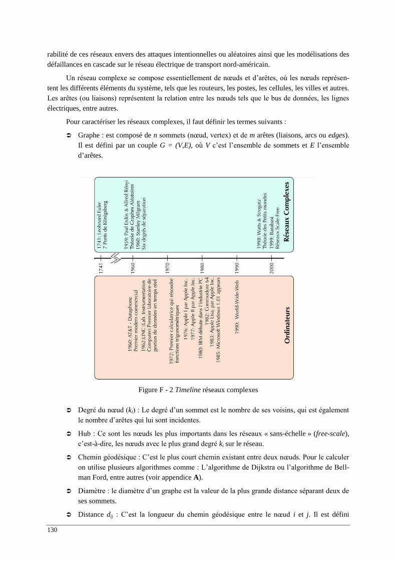
130
rabilité de ces réseaux envers des attaques intentionnelles ou aléatoires ainsi que les modélisations des défaillances en cascade sur le réseau électrique de transport nord-américain.
Un réseau complexe se compose essentiellement de nœuds et d’arêtes, où les nœuds représen-tent les différents éléments du système, tels que les routeurs, les postes, les cellules, les villes et autres. Les arêtes (ou liaisons) représentent la relation entre les nœuds tels que le bus de données, les lignes électriques, entre autres.
Pour caractériser les réseaux complexes, il faut définir les termes suivants :
Graphe : est composé de n sommets (nœud, vertex) et de m arêtes (liaisons, arcs ou edges). Il est défini par un couple G = (V,E), où V c’est l’ensemble de sommets et E l’ensemble d’arêtes.
Degré du nœud (ki) : Le degré d’un sommet est le nombre de ses voisins, qui est également le nombre d’arêtes qui lui sont incidentes.
Hub : Ce sont les nœuds les plus importants dans les réseaux « sans-échelle » (free-scale), c’est-à-dire, les nœuds avec le plus grand degré ki sur le réseau.
Chemin géodésique : C’est le plus court chemin existant entre deux nœuds. Pour le calculer on utilise plusieurs algorithmes comme : L’algorithme de Dijkstra ou l’algorithme de Bell-man Ford, entre autres (voir appendice A).
Diamètre : le diamètre d’un graphe est la valeur de la plus grande distance séparant deux de ses sommets.
Distance dij : C’est la longueur du chemin géodésique entre le nœud i et j. Il est défini
Figure F - 2 Timeline réseaux complexes
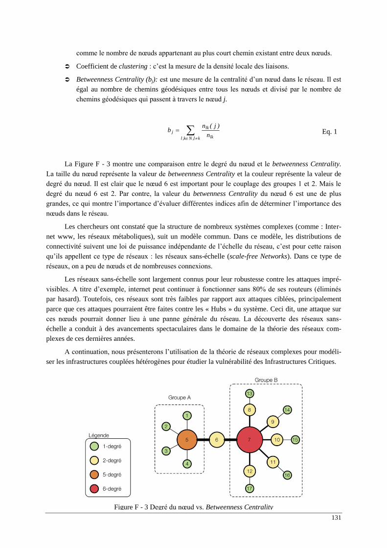
131
comme le nombre de nœuds appartenant au plus court chemin existant entre deux nœuds.
Coefficient de clustering : c’est la mesure de la densité locale des liaisons.
Betweenness Centrality (bj): est une mesure de la centralité d’un nœud dans le réseau. Il est égal au nombre de chemins géodésiques entre tous les nœuds et divisé par le nombre de chemins géodésiques qui passent à travers le nœud j.
kl,Nk,l lk
lkj
n
)j(nb Eq. 1
La Figure F - 3 montre une comparaison entre le degré du nœud et le betweenness Centrality. La taille du nœud représente la valeur de betweenness Centrality et la couleur représente la valeur de degré du nœud. Il est clair que le nœud 6 est important pour le couplage des groupes 1 et 2. Mais le degré du nœud 6 est 2. Par contre, la valeur du betwenness Centrality du nœud 6 est une de plus grandes, ce qui montre l’importance d’évaluer différentes indices afin de déterminer l’importance des nœuds dans le réseau.
Les chercheurs ont constaté que la structure de nombreux systèmes complexes (comme : Inter-net www, les réseaux métaboliques), suit un modèle commun. Dans ce modèle, les distributions de connectivité suivent une loi de puissance indépendante de l’échelle du réseau, c’est pour cette raison qu’ils appellent ce type de réseaux : les réseaux sans-échelle (scale-free Networks). Dans ce type de réseaux, on a peu de nœuds et de nombreuses connexions.
Les réseaux sans-échelle sont largement connus pour leur robustesse contre les attaques impré-visibles. A titre d’exemple, internet peut continuer à fonctionner sans 80% de ses routeurs (éliminés par hasard). Toutefois, ces réseaux sont très faibles par rapport aux attaques ciblées, principalement parce que ces attaques pourraient être faites contre les « Hubs » du système. Ceci dit, une attaque sur ces nœuds pourrait donner lieu à une panne générale du réseau. La découverte des réseaux sans-échelle a conduit à des avancements spectaculaires dans le domaine de la théorie des réseaux com-plexes de ces dernières années.
A continuation, nous présenterons l’utilisation de la théorie de réseaux complexes pour modéli-ser les infrastructures couplées hétérogènes pour étudier la vulnérabilité des Infrastructures Critiques.
Figure F - 3 Degré du nœud vs. Betweenness Centrality
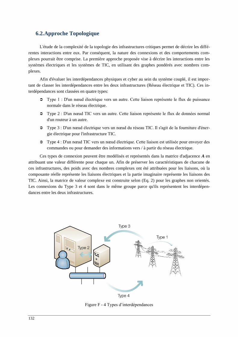
132
6.2. Approche Topologique
L'étude de la complexité de la topologie des infrastructures critiques permet de décrire les diffé-rentes interactions entre eux. Par conséquent, la nature des connexions et des comportements com-plexes pourrait être comprise. La première approche proposée vise à décrire les interactions entre les systèmes électriques et les systèmes de TIC, en utilisant des graphes pondérés avec nombres com-plexes.
Afin d'évaluer les interdépendances physiques et cyber au sein du système couplé, il est impor-tant de classer les interdépendances entre les deux infrastructures (Réseau électrique et TIC). Ces in-terdépendances sont classées en quatre types:
Type 1 : D'un nœud électrique vers un autre. Cette liaison représente le flux de puissance normale dans le réseau électrique.
Type 2 : D'un nœud TIC vers un autre. Cette liaison représente le flux de données normal d'un routeur à un autre.
Type 3 : D'un nœud électrique vers un nœud du réseau TIC. Il s'agit de la fourniture d'éner-gie électrique pour l'infrastructure TIC.
Type 4 : D'un nœud TIC vers un nœud électrique. Cette liaison est utilisée pour envoyer des commandes ou pour demander des informations vers / à partir du réseau électrique.
Ces types de connexion peuvent être modélisés et représentés dans la matrice d'adjacence A en attribuant une valeur différente pour chaque un. Afin de préserver les caractéristiques de chacune de ces infrastructures, des poids avec des nombres complexes ont été attribuées pour les liaisons, où la composante réelle représente les liaisons électriques et la partie imaginaire représente les liaisons des TIC. Ainsi, la matrice de valeur complexe est construite selon (Eq. 2) pour les graphes non orientés. Les connexions du Type 3 et 4 sont dans le même groupe parce qu'ils représentent les interdépen-dances entre les deux infrastructures.
Figure F - 4 Types d’interdépendances

133
contraire cas
4ou 3 est type (link si
2 est type (link si
1 est type (link si
0
11
1
1
)j,h
)j,h
)j,h
i
iahj Eq. 2
Par ailleurs, afin de tenir compte de la direction du flux d'informations et l'électricité, nous avons proposé une définition pour les graphes orientés. En effet, les graphes orientés sont capables de représenter la relation entre la source (les opérateurs) et la charge (les consommateurs finaux), où le premier offre un service à la seconde. L’entrée ahj est définie comme dans l’Eq. 3. Cette définition permet de créer un graphe mixte avec quelques liaisons avec un double sens, pour représenter l'appro-visionnement énergétique des réseaux de distribution et le flux de données du système TIC.
contraire cas
4ou 2 est type (link si
3ou 1 est type (link si
0
1
1
)j,h
)j,h
iahj Eq. 3
6.2.1. Degré des Nœuds
Afin d'identifier les vulnérabilités des infrastructures couplés, cette thèse vise à identifier les nœuds les plus importants dans le système, le terme «importance» est destinée à qualifier le rôle qui joue chaque nœud par rapport à sa présence et/ou l'emplacement par rapport à la moyenne globale et les propriétés du réseau. Le degré des nœuds est l'une des propriétés les plus communes des réseaux complexes afin d'identifier le rôle de chaque nœud dans le réseau, dans le cas spécifique de cette thèse, nous avons séparé le degré du nœud en deux parties : le degré du nœud électrique (hek), qui est le nombre de liaisons électriques incidentes avec le nœud k, et le degré du nœud TIC (kch) est le nombre de liaisons TIC incidentes avec le nœud h, Eq. 4.
hh ce
Vj
hjh kikak Eq. 4
Pour les graphes orientés, nous proposons deux définitions : in-degré et out-degré, voir Eq. 5 et Eq. 6.
inc
ine
Vj
hjinh hh
kikak Eq. 5
outc
oute
Vj
jhouth hh
kikak Eq. 6
6.2.2. Betweenness Centrality
La nature du réseau a une influence sur l'importance des liaisons et des nœuds dans le réseau. Cette nature est liée essentiellement par la fonction topologique de chaque composante du réseau. Les indices de centralité ont permis de mesurer cette importance.
Un de ces indices est le Betweenness Centrality. Depuis son origine, cet indice a été utilisé dans les études de la croissance urbaine, la résilience et la sociologie, en plus de son utilité dans l'identifica-tion des embouteillages et l’identification des liaisons / nœuds importants dans un réseau.
Nous proposons de calculer le Betweenness Centrality avec l’Eq. 7 pour les liens type 1 et 3, et
134
avec l’Eq. 8 pour les liens type 2 et 4.
jh,Vj,h hl,e
hl,ee
)l()l(b
Eq. 7
jh,Vj,h hl,c
hl,cc
)l()l(b
Eq. 8
Où hj est le nombre de chemins géodésiques entre h et j, et hj(l) est le nombre de chemins géodésiques entre h et j qui passent par l.
Un chemin géodésique dans la théorie des graphes est défini comme le plus court chemin exis-tant entre deux nœuds du graphe. Sa valeur dépend des pondérations éventuelles du graphe. Si le graphe est pondéré, une matrice de poids W est définie, dont l'entrée whj est le poids associé à la liaison entre les nœuds h et j. Sinon, la matrice d'adjacence est utilisée pour évaluer les chemins géodésiques. Il y a différent algorithmes de calcul des chemins géodésiques selon les propriétés du graphe et selon le problème considéré. Néanmoins, les plus populaires sont les algorithmes de Moore-Dijkstra et de Bellman (voir l’annexe A).
L’analyse des infrastructures couplées exige le calcul de deux chemins géodésiques, une pour chaque système (Réseau Electrique et Réseau TIC), défini comme hje (pour les poids réels) et hjc (pour les poids imaginaires), respectivement.
Nous avons défini l’indice de Betweenness Centrality global b(l) par l’Eq. 9.
)l(b)l(b)l(b ce22 Eq. 9
L’indice pour les liaisons (links) est défini par l’Eq. 10 et l’Eq. 11, pour les liaisons type 1 et 3 et type 2 et 4, respectivement.
jh,Vj,h hl,e
hl,ee
)e()e(b
Eq. 10
jh,Vj,h hl,c
hl,cc
)e()e(b
Eq. 11
6.2.3. L’efficacité
Un autre indice pour identifier les nœuds importants est l'efficacité. Le concept de l'efficacité a été introduit par (Latora et Marchiori 2001). Il est utilisé pour évaluer et mesurer l'efficacité d'un échange d'informations entre nœuds. Cet indice suppose que l'efficacité est inversement proportion-nelle à la distance la plus courte.
Pour notre cas, l’indice d'efficacité peut donner des indications sur l'impact de la suppression
135
d'un nœud (soit du côté TIC ou du réseau électrique) dans l’efficacité de communication et l'efficacité électrique du système, en parlant des topologies. Eq. 12 et Eq. 13 permettent d'évaluer l'efficacité des deux infrastructures. Où ne est le nombre de nœuds électriques et nc le nombre de nœuds TIC.
jh,Vj,Vh hjcec
ecdnn
E11
Eq. 12
jh,Vj,Vh hjcee
cednn
E11
Eq. 13
Si l’efficacité est faible, la distance dhj est plus élevée, cela signifie que le système est moins ef-ficace et donc le nœud supprimé joue un rôle important ou crucial dans le comportement du système.
6.2.4. Système de Test
Le système d'essai est un réseau de distribution très utilisé au sein du laboratoire G2ELAB et fait partie du plusieurs projets Européens et nationaux. Le réseau électrique possède 14 nœuds élec-triques, 17 lignes, 7 sources de production décentralisée, 9 charges et 3 transformateurs HTB/HTA, comme le montre la Figure F - 5.
En dehors de ce réseau, il existe une infrastructure de soutien considérable des TIC, une Wimax BS et 5 multiplexeurs, 23 liens, y compris ADSL, RTC / RNIS, fibre optique et les technologies Ethernet. Il y a aussi un réseau Ethernet LAN privé reliant les nœuds électriques 2, 3 et 4 (représenté par le nœud 23). Ce réseau de communication a été développé au cours du projet SINARI, il peut être un réseau privé ou public.
D’un côté, la Figure F - 7 montre le graphe non-orienté qui représente le système couplé. D’un autre côté, la Figure F - 8 représente le graphe orienté du système. Afin d’obtenir la direction des flux, nous avons utilisé les résultats de l’étude de répartition de charges du réseau électrique. Les différentes couleurs montrent les différents types de connexion entre les nœuds (type 1, 2, 3 et 4).
Grâce à cette représentation, nous pouvons calculer les différents indices présentés dans la der-nière section. A manière de résumé, les résultats obtenus sont montrés dans la prochaine section.
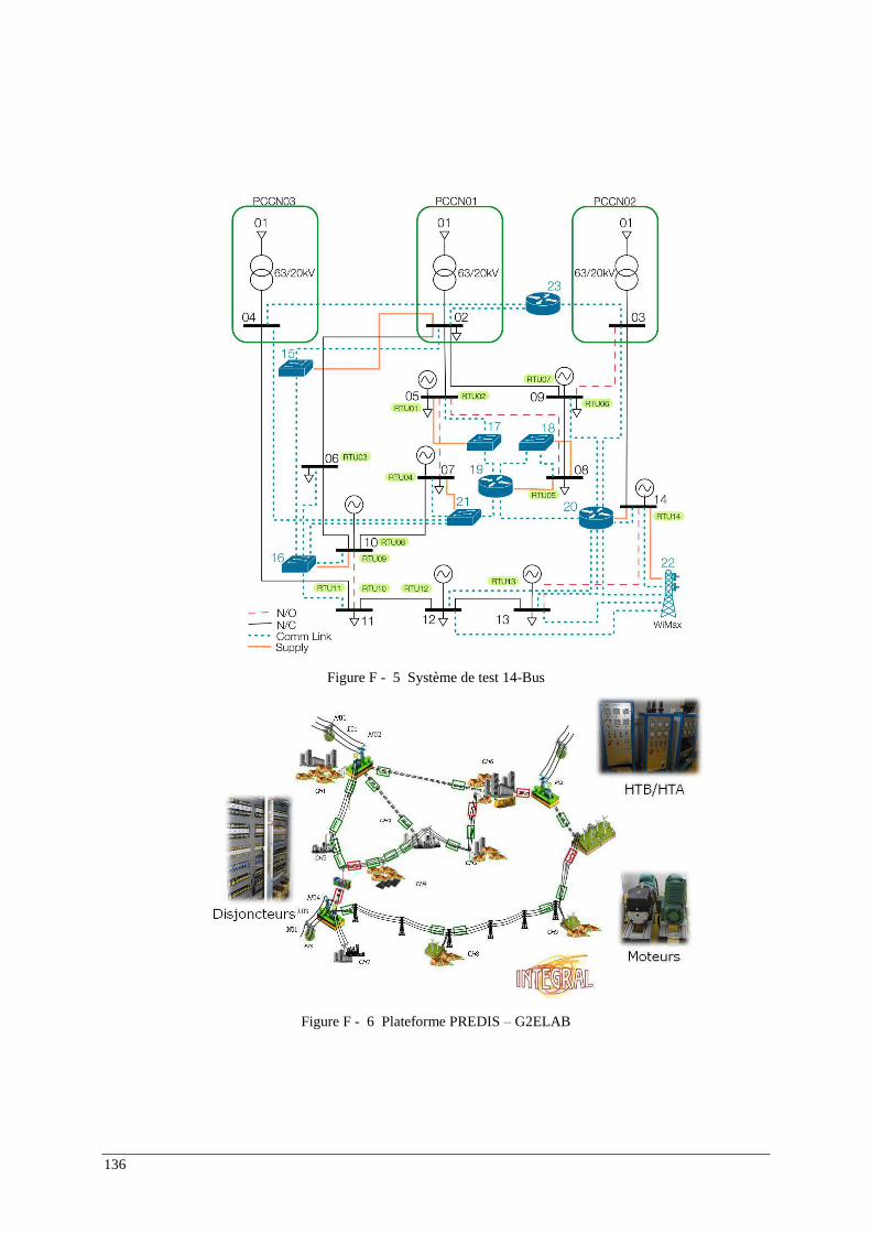
136
Figure F - 5 Système de test 14-Bus
Figure F - 6 Plateforme PREDIS – G2ELAB
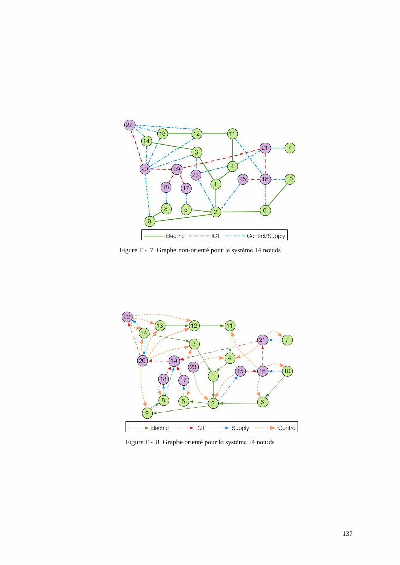
137
Figure F - 7 Graphe non-orienté pour le système 14 nœuds
Figure F - 8 Graphe orienté pour le système 14 nœuds
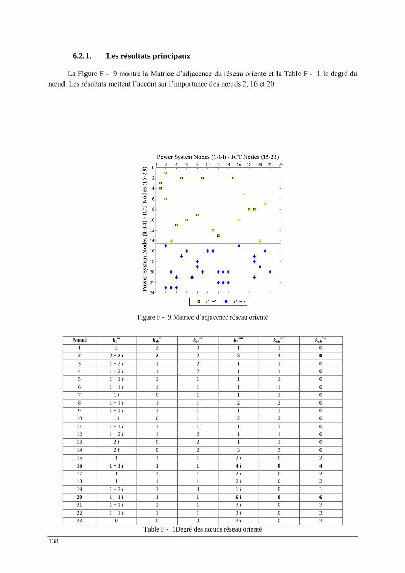
138
6.2.1. Les résultats principaux
La Figure F - 9 montre la Matrice d’adjacence du réseau orienté et la Table F - 1 le degré du nœud. Les résultats mettent l’accent sur l’importance des nœuds 2, 16 et 20.
Figure F - 9 Matrice d’adjacence réseau orienté
Nœud khin keh
in kchin kh
out kehout kch
out 1 2 2 0 1 1 0
2 2 + 2 i 2 2 3 3 0 3 1 + 2 i 1 2 1 1 0
4 1 + 2 i 1 2 1 1 0
5 1 + 1 i 1 1 1 1 0
6 1 + 1 i 1 1 1 1 0
7 1 i 0 1 1 1 0
8 1 + 1 i 1 1 2 2 0
9 1 + 1 i 1 1 1 1 0
10 1 i 0 1 2 2 0
11 1 + 1 i 1 1 1 1 0
12 1 + 2 i 1 2 1 1 0
13 2 i 0 2 1 1 0
14 2 i 0 2 3 3 0
15 1 1 1 2 i 0 2
16 1 + 1 i 1 1 4 i 0 4 17 1 1 1 2 i 0 2
18 1 1 1 2 i 0 2
19 1 + 3 i 1 3 1 i 0 1
20 1 + 1 i 1 1 6 i 0 6 21 1 + 1 i 1 1 3 i 0 3
22 1 + 1 i 1 1 3 i 0 3
23 0 0 0 3 i 0 3
Table F - 1Degré des nœuds réseau orienté
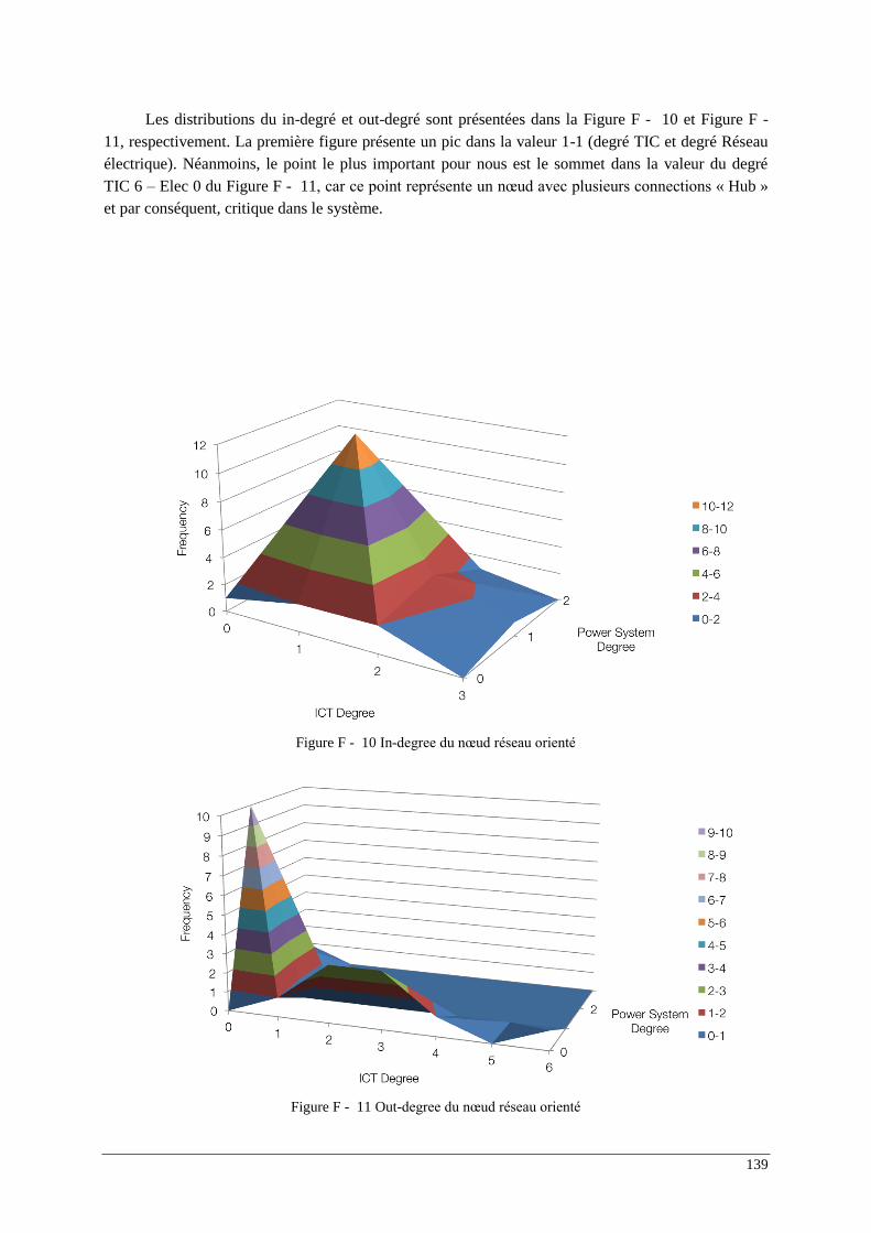
139
Les distributions du in-degré et out-degré sont présentées dans la Figure F - 10 et Figure F - 11, respectivement. La première figure présente un pic dans la valeur 1-1 (degré TIC et degré Réseau électrique). Néanmoins, le point le plus important pour nous est le sommet dans la valeur du degré TIC 6 – Elec 0 du Figure F - 11, car ce point représente un nœud avec plusieurs connections « Hub » et par conséquent, critique dans le système.
Figure F - 10 In-degree du nœud réseau orienté
Figure F - 11 Out-degree du nœud réseau orienté
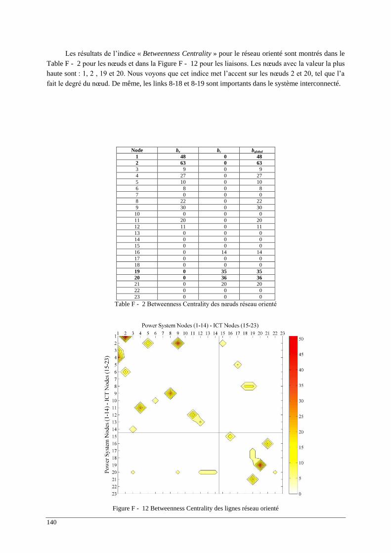
140
Les résultats de l’indice « Betweenness Centrality » pour le réseau orienté sont montrés dans le Table F - 2 pour les nœuds et dans la Figure F - 12 pour les liaisons. Les nœuds avec la valeur la plus haute sont : 1, 2 , 19 et 20. Nous voyons que cet indice met l’accent sur les nœuds 2 et 20, tel que l’a fait le degré du nœud. De même, les links 8-18 et 8-19 sont importants dans le système interconnecté.
Node be bc bglobal 1 48 0 48 2 63 0 63 3 9 0 9 4 27 0 27 5 10 0 10 6 8 0 8 7 0 0 0 8 22 0 22 9 30 0 30 10 0 0 0 11 20 0 20 12 11 0 11 13 0 0 0 14 0 0 0 15 0 0 0 16 0 14 14 17 0 0 0 18 0 0 0 19 0 35 35 20 0 36 36 21 0 20 20 22 0 0 0 23 0 0 0
Table F - 2 Betweenness Centrality des nœuds réseau orienté
Figure F - 12 Betweenness Centrality des lignes réseau orienté

141
L’Efficacité pour les nœuds est montrée dans la Figure F - 13 et pour les liens dans la Figure F - 14. Les nœuds importants à retenir sont 1, 2, 8, 19, 20 et 21. Ainsi que les liens au tour les nœuds 2 et 20.
C’est claire que les résultats obtenus grâce au degré du nœud, betwenness centrality et l’efficacité sont très similaires et permettent d’identifier des nœuds importants, tels que le nœud 2 et le nœud 20.
Figure F - 13 Efficacité des nœuds
Figure F - 14 Efficacité des lignes
0%
10%
20%
30%
40%
50%
60%
1 2 3 4 5 6 7 8 9 10 11 12 13 14 15 16 17 18 19 20 21 22 23
Electric Efficiency
Comm. Efficiency
0%
10%
20%
30%
40%
50%
60%
1-2
3-1
4-1
2-5
6-2
2-9
9-8
10-6
14-3
11-4
12-1
113
-12
7-21
10-1
65-
178-
188-
1914
-20
2-15
14-2
215
-16
15-2
20-1
421
-716
-10
17-5
18-8
16-2
116
-11
21-1
921
-423
-223
-323
-417
-19
18-1
919
-20
20-3
20-1
220
-13
20-2
222
-14
22-1
322
-12
20-9
16-6
Electric Drop Efficiency Comm Drop Efficiency

142
6.3. L’approche Spectrale
Les systèmes électriques et les infrastructures TIC ont des patrons asymétriques, c’est-à-dire, ces infrastructures ont diffèrent façons de partager l'information dans son propre réseau (électricité pour le premier et de données pour le second). Ce genre de modes de communication se trouve dans les réseaux sociaux où les personnes interagissent selon certaines règles sociales et utilisent différents canaux de communication, tels que les ordinateurs ou Smart phones. L’Approche Spectrale applique l’analyse Eigenspectral des systèmes pour étudier la structure des graphes pondérés orientés et asymé-triques afin d’exposer les vulnérabilités couplés.
(Hoser 2005) a proposé une méthode pour évaluer les réseaux asymétriques dans le contexte de la communication humaine, à l'aide des opérateurs linéaires dans l'espace de Hilbert en utilisant des matrices Hermitiennes. Cette section propose d'utiliser cette théorie pour l'étude des infrastructures interdépendantes. Dans un premier temps, il est proposé de distinguer les couches du système, où chaque niveau représente chaque type d’interdépendance, comme dans la Figure F - 15.
Après, la matrice d’admittance A est construit, pour chaque couche avec l’Eq. 14. Soit w le
nombre de liens sortants du nœud h vers le nœud j, et x le nombre de liens entrants provenant de nœud h vers le nœud j. Le graphe G(V,E) représente le système couplé, où V={Ve,Vc}.
xiwahj Eq. 14
6.3.1. Le degré complexe des Nœuds
Le degré ke est un nombre complexe où y est le nombre de liens sortant et z le nombre liens qui entrent dans le nœud, voir Eq. 15.
ziyakVj
hjh Eq. 15
Pareil à la première approche, ce degré permet de quantifier la dépendance de chaque nœud dans le système. Autrement dit, un nœud h peut savoir combien de nœuds en dépendent (nombre de liens qui partent de ce nœud) et le nombre de nœuds qui dépendent du nœud h (le nombre de liens qui sont pointées vers le nœud h). Une haute valeur du degré de nœud veut dire que plus de nœuds dépen-
Figure F - 15 Analyse multi-couche
143
dent / ou cela dépend de beaucoup d'autres nœuds. Par conséquent, un classement des degrés les plus élevés peut être fait et les premiers nœuds sont les plus critiques ou importantes pour le système.
6.3.2. La centralité spectrale
L’analyse spectrale permet d'identifier les connexions les plus faibles dans le système intercon-necté. L'analyse Eigenspectral sur des matrices d’adjacence de valeurs complexes peut être développée grâce à l'utilisation de matrices Hermitiennes dans l'espace de Hilbert.
Par conséquent, la matrice d’adjacence doit être une matrice Hermitienne dans l'espace de Hil-bert. Comme la matrice d’adjacence a la caractéristique présentée dans Eq. 16, la matrice hermitienne peut être construite selon Eq. 17.
jhhj aia Eq. 16
4
i
eAH Eq. 17
Enfin, les vecteurs propres et les valeurs propres des matrices hermitiennes sont calculés selon Eq. 18 pour chaque matrice d’adjacence, représentant chaque interdépendance. Le nœud le plus impor-tant dans le système est identifié en fonction de la plus grande valeur absolue dans le vecteur propre en cours d'inspection.
xHx Eq. 18
6.3.3. Les résultats principaux
Le même système de test est utilisé pour illustrer l'application de la théorie spectrale. La Figure F - 16 montre comment le réseau de test est représenté à l'aide des réseaux complexes en deux ni-veaux, l'un pour réseau électrique et l'autre pour le réseau TIC. Le réseau électrique est représenté avec des liens directionnels et le réseau de communication est représenté par des liaisons bidirectionnelles. Chacune de ces couches seront représentées avec un adjacence de matrice et leurs valeurs seront cal-culées pour déterminer les nœuds du système les plus critiques.
La Table F - 3 montre les résultats obtenus après avoir calculé les vecteurs et valeurs propres. Dans ce cas, les nœuds les plus critiques sont le nœud 1 et 2 pour le réseau électrique, et au nœud 20 et 22 pour le réseau de communication. Ils sont les mêmes résultats obtenus par l'analyse topologique du système (voir la section précédente). De même, il est important de constater que des valeurs nulles représentent les éléments qui n'ont pas une dépendance du système. Ceci a permis l'identification des îlots dans le système.
L'un des principaux avantages de ce type d'analyse est qu'elle permet d'intégrer dans un seul modèle, le comportement de chaque infrastructure hétérogène.
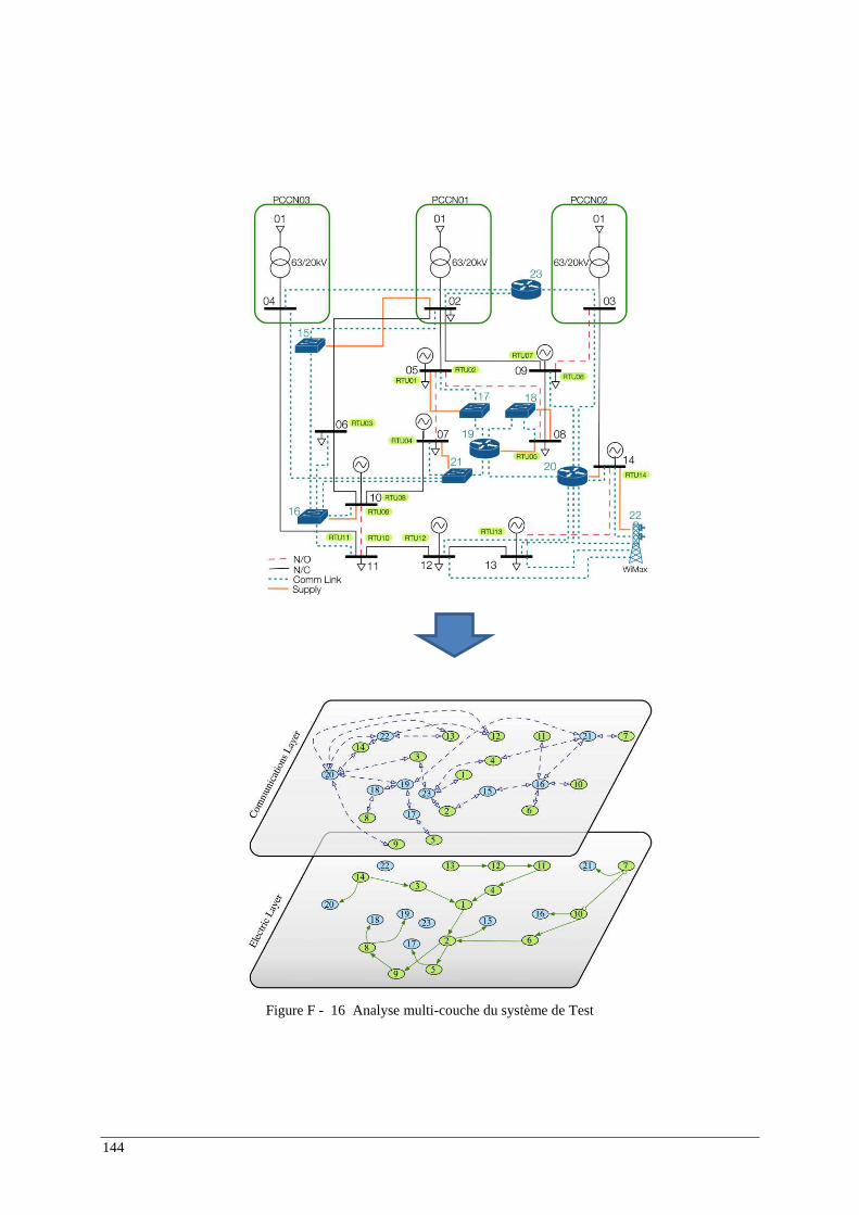
144
Figure F - 16 Analyse multi-couche du système de Test
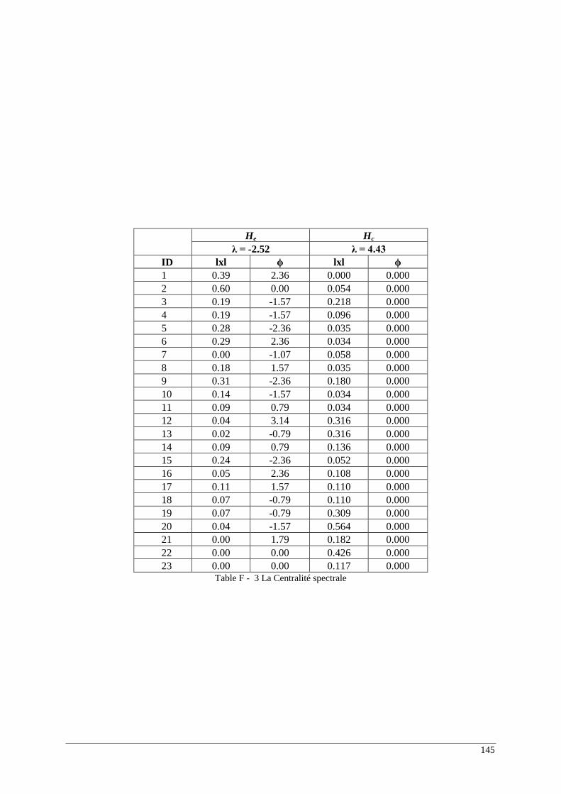
145
He Hc
λ = -2.52 λ = 4.43 ID lxl ϕ lxl ϕ 1 0.39 2.36 0.000 0.000 2 0.60 0.00 0.054 0.000 3 0.19 -1.57 0.218 0.000 4 0.19 -1.57 0.096 0.000 5 0.28 -2.36 0.035 0.000 6 0.29 2.36 0.034 0.000 7 0.00 -1.07 0.058 0.000 8 0.18 1.57 0.035 0.000 9 0.31 -2.36 0.180 0.000 10 0.14 -1.57 0.034 0.000 11 0.09 0.79 0.034 0.000 12 0.04 3.14 0.316 0.000 13 0.02 -0.79 0.316 0.000 14 0.09 0.79 0.136 0.000 15 0.24 -2.36 0.052 0.000 16 0.05 2.36 0.108 0.000 17 0.11 1.57 0.110 0.000 18 0.07 -0.79 0.110 0.000 19 0.07 -0.79 0.309 0.000 20 0.04 -1.57 0.564 0.000 21 0.00 1.79 0.182 0.000 22 0.00 0.00 0.426 0.000 23 0.00 0.00 0.117 0.000
Table F - 3 La Centralité spectrale
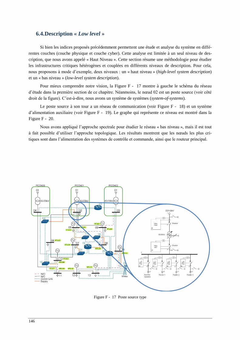
146
6.4. Description « Low level »
Si bien les indices proposés précédemment permettent une étude et analyse du système en diffé-rentes couches (couche physique et couche cyber). Cette analyse est limitée à un seul niveau de des-cription, que nous avons appelé « Haut Niveau ». Cette section résume une méthodologie pour étudier les infrastructures critiques hétérogènes et couplées en différents niveaux de description. Pour cela, nous proposons à mode d’exemple, deux niveaux : un « haut niveau » (high-level system description) et un « bas niveau » (low-level system description).
Pour mieux comprendre notre vision, la Figure F - 17 montre à gauche le schéma du réseau d’étude dans la première section de ce chapitre. Néanmoins, le nœud 02 est un poste source (voir côté droit de la figure). C’est-à-dire, nous avons un système de systèmes (system-of-systems).
Le poste source à son tour a un réseau de communication (voir Figure F - 18) et un système d’alimentation auxiliaire (voir Figure F - 19). Le graphe qui représente ce niveau est montré dans la Figure F - 20.
Nous avons appliqué l’approche spectrale pour étudier le réseau « bas niveau », mais il est tout à fait possible d’utiliser l’approche topologique. Les résultats montrent que les nœuds les plus cri-tiques sont dans l’alimentation des systèmes de contrôle et commande, ainsi que le routeur principal.
Figure F - 17 Poste source type
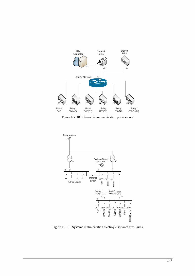
147
Figure F - 18 Réseau de communication poste source
Figure F - 19 Système d’alimentation électrique services auxiliaires
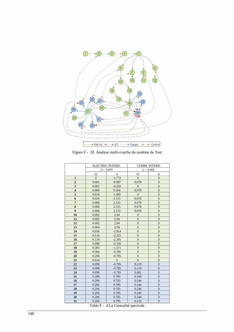
148
Figure F - 20 Analyse multi-couche du système de Test
ELECTRIC INTERD. COMM. INTERD λ = 3.079 λ = 4.402
|x| φ |x| φ 1 0 -1.772 0 0 2 0.001 -0.987 0.078 0 3 0.002 -0.202 0 0 4 0.006 0.584 0.078 0 5 0.016 1.369 0 0 6 0.026 2.155 0.078 0 7 0.006 2.155 0.078 0 8 0.006 2.155 0.078 0 9 0.006 2.155 0.078 0 10 0.002 2.94 0 0 11 0.002 2.94 0 0 12 0.002 2.94 0 0 13 0.064 2.94 0 0 14 0.056 -2.914 0 0 15 0.116 -2.321 0 0 16 0.119 -2.391 0 0 17 0.098 -2.356 0 0 18 0.303 -1.571 0 0 19 0.304 -0.785 0 0 20 0.206 -0.785 0 0 21 0.634 0 0 0 22 0.098 -0.785 0.219 0 23 0.098 -0.785 0.219 0 24 0.098 -0.785 0.681 0 25 0.206 0.785 0.244 0 26 0.206 0.785 0.244 0 27 0.206 0.785 0.244 0 28 0.206 0.785 0.244 0 29 0.206 0.785 0.244 0 30 0.206 0.785 0.244 0 31 0.206 0.785 0.219 0
Table F - 4 La Centralité spectrale
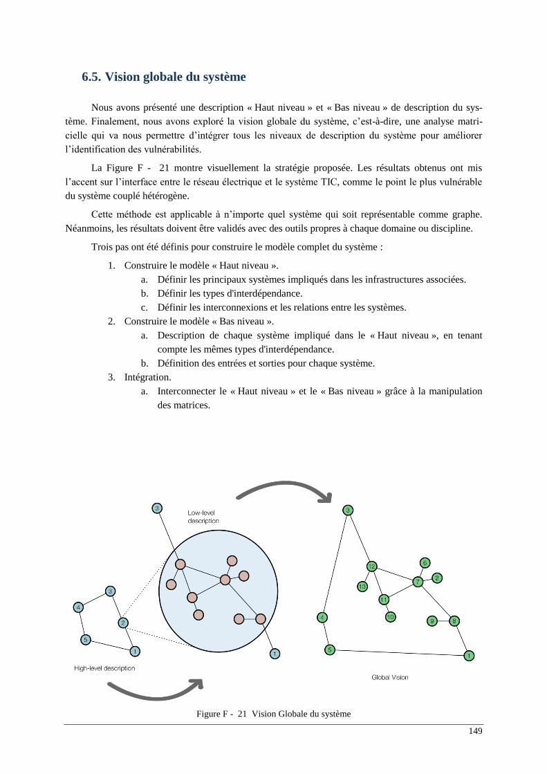
149
6.5. Vision globale du système
Nous avons présenté une description « Haut niveau » et « Bas niveau » de description du sys-tème. Finalement, nous avons exploré la vision globale du système, c’est-à-dire, une analyse matri-cielle qui va nous permettre d’intégrer tous les niveaux de description du système pour améliorer l’identification des vulnérabilités.
La Figure F - 21 montre visuellement la stratégie proposée. Les résultats obtenus ont mis l’accent sur l’interface entre le réseau électrique et le système TIC, comme le point le plus vulnérable du système couplé hétérogène.
Cette méthode est applicable à n’importe quel système qui soit représentable comme graphe. Néanmoins, les résultats doivent être validés avec des outils propres à chaque domaine ou discipline.
Trois pas ont été définis pour construire le modèle complet du système :
1. Construire le modèle « Haut niveau ». a. Définir les principaux systèmes impliqués dans les infrastructures associées. b. Définir les types d'interdépendance. c. Définir les interconnexions et les relations entre les systèmes.
2. Construire le modèle « Bas niveau ». a. Description de chaque système impliqué dans le « Haut niveau », en tenant
compte les mêmes types d'interdépendance. b. Définition des entrées et sorties pour chaque système.
3. Intégration. a. Interconnecter le « Haut niveau » et le « Bas niveau » grâce à la manipulation
des matrices.
Figure F - 21 Vision Globale du système
150
7. Conclusions et Perspectives
Les réseaux électriques actuels sont fortement dépendants des systèmes TIC à différents ni-veaux y compris les systèmes de capteurs sur le terrain, au niveau de centres de commande et incluent les moyens de communication avec le marché d’électricité et les autres systèmes de contrôle (systèmes voisins). Ils sont utilisés pour l’acquisition d'informations ainsi que pour la contrôle-commande qui sont vitales pour la surveillance du système. L'intégration efficace des TIC dans les réseaux électriques doit conduire à un fonctionnement plus optimisé et un meilleur contrôle de ces systèmes pour, ainsi, accroître l'efficacité générale. Par ailleurs, les TICs sont des éléments et fonctions clés dans la re-cherche et le développement des «Smart Grids».
Bien que les systèmes TIC et les réseaux électriques ont été conçus à des fins et des contextes différents, ces infrastructures sont fortement dépendantes aujourd’hui. D'autre part, le besoin d'interac-tion entre les différents acteurs du système, a donné lieu à de nouvelles vulnérabilités, ce qui rend les interdépendances entre les infrastructures de plus en plus critiques.
Par conséquent, il est primordial de considérer les infrastructures couplées et interdépendantes et hétérogènes dans la modélisation, la conception et l'analyse de sécurité. Dans ce contexte, la modé-lisation des interdépendances est considérée comme une condition préalable pour sécuriser ces infras-tructures. Le résultat attendu de cette vision est que les systèmes TIC peuvent, non seulement, rendre le réseau électrique plus résilient, mais aussi plus efficace tout en permettant aux acteurs du système d’y être plus impliqués, y compris les consommateurs finaux. Par ailleurs, le résultat peut faciliter l'intégration des sources d'énergie renouvelables en fournissant, par exemple, efficacité, rentabilité et des solutions sécurisées pour surveiller et contrôler les générateurs dispersés de petite taille. De cette façon, les TICs contribueraient aussi à la protection contre le changement climatique.
Une modélisation unifiée est nécessaire afin de pouvoir appréhender au mieux le comportement émergeant des systèmes couplés. Les principales difficultés de cette thèse ont pour origine l’hétérogénéité des systèmes étudiés et la nouveauté scientifique de ce sujet. En effet, le travail présen-té est précurseur dans ce domaine avec l’étude couplée des réseaux électriques et de communication associés.
La proposition de modélisation possède quelques limitations dues à l’ensemble des hypothèses considérées. Ainsi, les développements actuels buttent sur des études uniquement statiques. Des déve-loppements futurs devraient intégrer, au sein même des réseaux complexes, des équations différen-tielles.
Néanmoins, les méthodes proposées sont originales, adaptées à l’étude d’infrastructures cri-tiques susceptibles à l’effet de cascade et surtout à des systèmes multi-infrastructures. Les résultats obtenus, suite à la modélisation des interdépendances des infrastructures critiques, permettent de pro-gresser dans la compréhension du comportement des systèmes couplés. Cette progression dans la compréhension participe ainsi au but de sécurisation des infrastructures critiques.
151
BIBLIOGRAPHY
ABB Inc. Toward a Smarter grid: ABB's vision for the power system of the future. ABB White paper, ABB, 2009.
Abraham, Sherly, and InduShobha Chergalur-Smith. "An overview of social engineering malware: Trends, tactics, and implications." Technology in Society 32, no. 3 (August 2010): 183-196.
Ahmed, Mariam, Ahmad Hably, and Seddik Bacha. "Kite Generator System Modeling and Grid Integration." IEEE Transactions on Sustainable Energy, 2013.
Albert, Réka, and Albert-Laszlo Barabasi. "Statistical mechanics of complex networks." Reviews of Modern
Physics, no. 74 (2002): 47-97.
Albert, Réka, Hawoong Jeong, and Albert-Laszlo Barabasi. "Error and attack tolerance of complex networks." Nature 406 (July 2000): 378-382.
ANSSI. Référentiel Général de Sécurité. Paris: Agence nationale de la sécurité des systèmes d'information, 2010.
Barabási, Albert-Lázló, and Eric Bonabeu. "Scale-Free networks." Scientific American 288, no. 5 (2003): 60-69.
Barabási, Albert-Lázlo, and Réka Albert. "Emergence of scaling in random networks." Science 286 (1999): 509-512.
Barrat, Alain, Marc Barthélemy, and Alessandro Vespignani. Dynamical Processes on Complex Networks. Cambridge: Cambridge University Press, 2012.
Beccuti, Marco, Silvano Chiaradonna, Felicita Di Giandomenico, Susanna Donatelli, Giovanna Dondossola, and Giuliana Franceschinis. "Quantification of dependencies between electrical and information infrastructures." International Journal of Critical Infrastructure Protection 5 (2012): 14-27.
Benbow, Donald, and Hugh Broome. The Certified Reliability Engineer Handbook. Milwaukee: ASQ, 2009.
Birolini, Alessandro. Reliability Engineering: Theory and Practice. Springer, 2007.
Boardman, John, and Brian Saucer. System Thinking: Coping with 21st century problems. Boca Raton: CRC Press, 2008.
Boccaletti, S., V. Latora, Y. Moreno, M. Chavez, and D.-U. Hwang. "Complex networks: Structure and dynamics." Physics Reports 424 (2006): 175-308.
Bompard, Ettore, Ciwei Gao, Roberto Napoli, Angela Russo, Marcelo Masera, and Alberto Stefanini. "Risk Assessment of Malicious Attacks Against Power Systems." IEEE Transactions on Systems, Mand and
Cybernetics - Part A 39, no. 5 (2009): 1074-1085.
Bompard, Ettore, Di Wu, and Fei Xue. "Structural vulnerability of power systems: A topological approach." Electric Power Systems Research 81 (2011): 1334-1340.
152
Bompard, Ettore, Paolo Cuccia, Marcelo Masera, and Igor Fovino. "Cyber Vulnerability in Power Systems Operation and Control." Critical Infrastructure Protection (Springer Berlin) 7130 (2012): 197-234.
Bonabeau, Eric. "Agent-based modeling: Methods and techniques for simulating human systems." Proc. of the
National Academy of Sciences of the USA. USA: National Academy of Sciences, 2002. 7280-7287.
Bouisson, Marc. "L'outil FIGSEQ de calcul par séquences." EDF Innovation. n.d. http://innovation.edf.com/recherche-et-communaute-scientifique/logiciels (accessed February 22, 2013).
Bouissou, Marc, and Jean-Louis Bon. "A new formalism that combines advantages of fault-trees and Markov models: Boolean logic driven markov processes." Reliability Engineering & System Safety 82 (2003): 149-163.
Brandes, Ulrik. "A faster algorithm for betweenness centrality." Journal of Mathematical Sociology 25, no. 2 (2001): 163-177.
Byres, Eric. "SCADA Security Basics: SCADA vs. ICS terminology." Tofino Security. September 05, 2012. http://www.tofinosecurity.com (accessed January 20, 2013).
Caire, Raphael, Jose Sanchez, and Nouredine Hadjsaid. "Vulnerability Analysis of Coupled Heterogeneous Critical Infrastructures: a Co-simulation approach with a testbed validation." IEEE PES Innovative
Smart Grid Technologies, Europe 2013. Copenhagen, 2013.
Caldarelli, Guido. Scale-Free Networks: Complex Webs in Nature and Technology. Oxford University Press: New York, 2007.
Casalicchio, Emiliano, Emanuele Galli, and Salvatore Tucci. "Federated Agent-Based modeling and simulation approach to study interdependencies in IT Critical Infrastructures." 11th IEEE Symposium on
Distributed Simulation and Real-Time applications. Chania, 2007. 182-189.
—. "Macro and micro agent-based modeling and simulation of critical infrastructures." 2010 Complexity in
Engineering. Rome, 2010. 79-81.
CEN-CENELEC-ETSI. "Smart Grid Coordination Group Smart Grid Reference Architecture." Brussels, 2012.
CERT. CERT advisory CA-2001-26 nimda worm. CERT, 2001.
Cheminod, Manuel, Luca Durante, and Adriano Valenzano. "Review of Security issues in industrial networks." IEEE Transactions on Industrial Informatics 9, no. 1 (2013): 277-293.
Chen, Thomas, and Abu-Nimeh Saeed. "Lessons from Stuxtnet." Computer (IEEE Computer Society), April 2011: 91-93.
Chen, Thomas, Juan Carlos Sanchez Aarnoutse, and John Buford. "Petri Net modeling of cyber-physical attacks on Smart Grid." IEEE Transactions on Smart Grid 2, no. 4 (2011): 741-749.
Chen, Wai-Kai. The Electrical Engineering Handbook. San Diego: Elsevier Academic Press, 2005.
Chiola, G, C. Dutheillet, G. Franceschinis, and S. Haddad. "Stochastic well-formed coloured nets for symmetric modelling applications." IEEE Transactions on Computers 42, no. 11 (1993): 1343-1360.
Chvatal, Vasek. Linear Programming. W.H. Freeman, 1983.
Cohen, Reuven, and Shlomo Havlin. Complex Networks: Structure, Robustness and Function. New York: Cambridge University Press, 2010.
Commission of the European Communities. Communication from the commission to the Council and the
European Parliament: Critical Infrastructure Protection in the fight against terrorism. Commission of the European Communities, 2004.
Cormen, Thomas, Charles Leiserson, Ronald Rivest, and Clifford Stein. Introduction to Algorithms. MIT Press, 2001.
Cruccitti, Paolo, Vito Latora, and Massimo Marchiori. "Model for cascading failures in complex networks."
153
Physical Review E 69, no. 045104 (2004).
De Porcellinis, S., R. Setola, Stefan Panzieri, and G. Ulivi. "Simulation of heterogeneous and interdependent critical infrastructures." International Journal of Critical Infrastructures 4, no. 1/2 (2008): 110-128.
Di Giorgio, Alessandro, and Francesco Liberati. "A Bayesian network-based approach to the critical infrastructure interdependencies analysis." IEEE Systems Journal 6, no. 3 (2012): 510-519.
Erdös, Paul, and Alfréd Rényi. "On random graphs." Publicationes Mathematicae Debrecen 6 (1959): 290-297.
Erdös, Paul, and Alfréd Rényi. "On the evolution of random graphs." Publi. Math. Inst. Hung. Acad. Sci. 5 (1960): 17-61.
EU Commission Task Force for Smart Grids. Expert Group 1: Functionalities of Smart Grids and Smart Meters. Final Delivrable, European Union Commission, 2010.
EU Project IRRIIS. "Tools and Techniques for interdependency analysis." Deliverable D222, June 2007, 4551.
Euler, Leonhard. "Solutio problematis ad geometriam situs pertinentis." Commentarii academiae scientiarum
Petropolitanae, no. 8 (1741): 128-140.
European Commission. Mandate 490: Standarization Mandate to European Standarisation Organisations to
support European Smart Grid deployment. Mandate, Brussels: Dictorate General for Energy, 2011.
European Union. Council Directive 2008/114/EC: on the identification and designation of European critical
infrastructures and the assessment of the need to improve their protection. Brussels: Official Journal of the European Union, 2008.
Eusgeld, Irene, Wolfgang Kröger, Giovanni Sansavini, Markus Schläpfer, and Enrico Zio. "The role of network theory and object-oriented modeling within a framework for the vulnerability analysis of critical infrastructures." Reliability Engineering & System Safety 94 (2009): 954-963.
Falliere, Nicolas, Liam Murchu, and Eric Chien. W.32 Stuxnet Dossier. Symantec, Cupertino: Symantec, 2011.
Fiedler, Miroslav. "Algebraic Connectivity of Graphs." Czechoslovak Mathematical Journal 23, no. 98 (1793): 298-305.
Franko, Kantele, and Jonathan Fahey. US electrical grid still vulnerable. The Associated Press. August 11, 2013. http://www.pressherald.com/business/u-s-electrical-grid-still-vulnerable-2013-08-11.html (accessed August 14, 2013).
Freeman, L.-C. "A set of measures of centrality based on betweenness." Sociometry, 1977: 35-41.
Galli, Emanuele. Agent Based Modeling and Simulation for Critical and interdependent systems. PhD Dissertation, Rome: Universita di Roma, 2010.
Galloway, Brendan, and Gerhard Hancke. "Introduction to Industrial Control Networks." IEEE Communications
Surveys & Tutorials, 2012: On press.
Gönen, Turan. Electric Power Distribution System Engineering. Boca Raton: Taylor & Francis Group, 2008.
Gorod, Alex, Brian Sauser, and John Boardman. "System-of-Systems Engineering Management: A review of Modern History and a path forward." IEEE Systems Journal 2, no. 4 (2008): 484-498.
GRID. "ICT Vulnerabilities of Power Systems: A Roadmap for Future Research." A coordination action on ICT vulnerabilities of power systems and the relevant defence methodologies, 2007.
Grigsby, Leonard L. Electric power generation, transmission, and distribution. Boca Raton: CRC Press, 2007.
Hadjsaid, Nouredine. ICT Vulnerabilities of Power Systems: A roadmap for Future Research. General Joint Research Centre, 2008.
Hadjsaid, Nouredine, and Jean-Claude Sabonnadière. Power Systems and Restructuring. London: iSTE - Wiley, 2009.
Hadjsaid, Nouredine, et al. "Integrated ICT framework for distribution network with decentralized energy

154
resources: Prototype, design and development." IEEE PES Society General Meeting. IEEE, 2010. 1-4.
Hadjsaid, Nouredine, J-F. Canard, and F. Dumas. "Dispersed generation impact on distribution networks." IEEE
Computer Applications in Power 12, no. 2 (1999): 22-28.
Haimes, Y., and P. Jiang. "Leontief-based model of risk in complex interconnected infrastructures." Journal of
Infrastructure Systems 7, no. 1 (2001): 1-12.
Halpin, Edward, Philippa Trevorrow, David Webb, and Steve Wright. Cyberwar, Netwar and the revolution in
military affairs. Basingstoke: Palgrave Macmillan, 2006.
Hewitson, Leslie, Mark Brown, and Ramesh Balakrishnan. Practical Power System Protection. Burlington: Elsevier - Newnes, 2005.
Hines, Paul, Eduardo Cotilla-Sanchez, and Seth Blumsack. "Do topological models provide good information about electricity infrastructure vulnerability?" Edited by American Institute of Physics. Chaos 20, no. 3 (2010): 033122.
Hopkinson, Kenneth, Xiaoru Wang, James Thorp Giovanini, and Kenneth Birman. "EPOCHS: A platform for Agent-Based electric power and communication simulation built from commercial off-the-Shelf Components." IEEE Transactions on Power Systems 21, no. 2 (2006): 548-558.
Hoser, Bettina. Analysis of Asymmetric Communication Patterns in Computer Mediated Communication
Environments. Karlsruhe: Universitätsverlag karlsruhe, 2005.
ICS-CERT. ICS-CERT Monitor. Monitor Report, U.S. Department of Homeland Security, 2012.
ICS-CERT. ICS-CERT Monitor report. ICS-CERT, April/May/June 2013.
IEC 61850. Communication networks and systems in substations. Technical Raport, Geneva: IEC, 2003.
Intech. Petri Nets Applications. Edited by Pawel Pawlewski. INTECH, 2010.
Jaeger, Carlo, Patrik Jansson, Sander van der Leeuw, Michael Resch, Juan David Tabara, and Ralph Dum. "Global Systems Science." Orientation paper, 2013.
Jeong, Hawoong, B. Tombor, Albert Réka, Z. Oltvai, and Albert-Laszlo Barabasi. "The large-scale organization of metabolic networks." Nature 407 (October 2000): 651-654.
Johansson, Jonas. Risk and Vulnerability Analysis of Interdependent Technical Infrastructures: Addressing Socio-Technical Systems. PhD Thesis, Lund: Lund University, 2010.
Johansson, Jonas, and Henrik Hassel. "An approach for modelling interdependent infrastructures in the context of vulnerability analysis." Reliability Engineering and System Safety 95 (2010): 1335-1344.
Karpersky Laboratory. "New investigation points to three flame-related malicious programs: at least one still in the wild." Karpersky. September 17, 2012. http://ww.Karpersky.com (accessed 25 12, 2013).
Keating, Charles, et al. "Systems of Systems engineering." Engineering Management Journal 15, no. 3 (2003): 36-45.
Khelil, Abdelmajid, Daniel Germanus, and Neeraj Suri. "Protection of SCADA Communication Channels." Critical Infrastructure Protection, 2012: 177-196.
Knapp, Eric. Industrial Network Security: Securing critical infrastructure networks for smart grid, SCADA, and
other Industrial Control Systems. Waltham: Elsevier, 2011.
Knight, Upton George. Power Systems in Emergencies: From contringency planning to crisis management. John Wiley & Sons, 2001.
Kriaa, Siwar, Marc Bouissou, and Piètre-Cambacédès. "Modeling the Stuxnet Attack with BDMP: Towards more formal risk assessments." 7th International Conference on Risk and Security on Internet and
Systems (CRiSIS). Cork, 2012.
Kröger, Wolfgang. "Critical Infrastructures at Risk, a need for a new conceptual approach and extended
155
analytical tools." Reliability Engineering & System Safety 93, no. 12 (2008): 1781-1787.
Kröger, Wolfgang, and Enrico Zio. Vulnerable Systems. New York: Springer, 2011.
Krutz, Ronald. Securing SCADA Systems. Indianapolis: Wiley, 2006.
Laprie, Jean-Claude, Karama Kanoun, and Mohamed Kaâniche. "Modelling Interdependencies between the Electricity and Information Infrastructures." Lecture Notes in Computer Science, September 2007: 54-67.
Latora, V., and M. Marchiori. "Efficient behavior of small-world networks." Physical Review Letters 87 (2001).
Leszczyna, Rafal, Igor Nai Fovino, and Marcelo Masera. "Approach to security assessment of critical infrastructures' information systems." IET Information Security 5, no. 3 (2010): 135-144.
Le-Thanh, L., Raphaël Caire, Bertrand Raison, Seddik Bacha, F. Blache, and G. Valla. "Test bench for self-healing functionalities applied on distribution network with distributed generators." IEEE PES
PowerTech. Bucharest, 2009. 1-6.
Liu, Chen-Ching, Alexandru Stefanov, Junho Hong, and Patrick Panciatici. "Intruders in the Grid." IEEE power
& Energy magazine, 2012: 58-66.
Liu, Nian, Jianhua Zhang, and Xu Wu. "Asset Analysis of Risk Assessment for IEC 61850-Based Power Control systems - Part I: Methodology." IEEE Transactions on Power Delivery 26, no. 2 (2011): 869-875.
Liu, Nian, Jianhua Zhang, and Xu Wu. "Asset Analysis of Risk Assessment for IEC 61850-Based Power Control Systems- Part II: Application in Substations." IEEE Transactions on Power Delivery 26, no. 2 (2011): 876-881.
Luiijf, Eric, Albert Nieuwenhuijs, Marieke Klaver, Michel van Eeten, and Edite Cruz. "Empirical Findings on Critical Infrastructure Dependencies in Europe." In Critical Infrastructure Security, by Roberto Setola and Stefan Geretshuber, 302-310. Rome: Springer, 2009.
Masera, Marcelo, Igor Nal Fovino, and Bogdan Vamanu. ICT aspects of power systems and their security. JCR Scientific and Technical Report, Luxembourg: JRC European Commission, 2011.
McDonald, John, et al. "The SINARI Project Security: Security Analysis and Risk Assessment applied to the Electrical Distribution Network." CIRED Conference. Stockholm, 2013.
Merdassi, Asma, et al. "Modeling methods coupled electrical networks and ICT. An inventory." European
Journal on Electrical Engineering 15/6 (2012): 557-585.
Milgram, Stanley. "The small world problem." Psychology today 2, no. 1 (1967): 60-67.
Mitchell, Robert, and Ing-Ray Chen. "Effect of intrusion detection and reponse on reliability of cyber physical systems." IEEE Transactions on Reliability 62, no. 1 (2013): 199-210.
Motorola. Cybersecurity managing the complexity. White Paper, Schaumburg: Motorola Solutions, 2012.
Müller, Sven, Hanno Georg, Christian Rehtanz, and Christian Witfeld. "Hybrid Simulation of Power Systems and ICT for Real-Time applications." 3rd IEEE PES Innovative Smart Grid Technologies Europe (ISGT
Europe). Berlin, 2012.
Murata, Tadao. "Petri Nets: Properties, analysis and applications." Proceedings of the IEEE, 1989: 541-580.
Nan, Cen, Irene Eusgeld, and Wolfgang Kröger. "Analyzing vulnerabilities between SCADA system and SUC due to interdependencies." Reliability Engineering & System Safety 113 (2013): 76-93.
Newman, Mark. "Complex Systems: A survey." American Journal of Physics 79 (2011): 800-810.
Newman, Mark. "The structure and function of complex networks." SIAM Review 45, no. 2 (2003): 167-256.
NIST. NIST framework and roadmap for Smart Grid Interoperability. National Institute of Standards and Technology, 2012.
Oliva, Gabriele, Stefano Panzieri, and Roberto Setola. "Agent-based input-output interdependency model."
156
International Journal of Critical Infrastructure Protection 3, no. 2 (2010): 76-82.
O'Rourke, Thomas Denis. "Critical Infrastructure, Interdependencies, and Resilience." The Bridge: Engineering
for the Threat of Natural Disasters 37, no. 1 (2007).
Ouyang, Min. "Review on Modeling and Simulation of Interdependent Critical Infrastructure Systems." Reliability engineering & System safety, 2013: [In Press].
Pearl, Judea, and Stuart Russell. "Bayesian Networks." In The Handbook of Brain Theory and Neural networks, by Michael Arbib, 157-160. Boston: MIT Press, 2003.
Peterson, Larry L., and Bruce Davie. Computer Networks: A systems approach. 3. San Francisco: Elsevier, 2003.
Petri, Carl. Kommunikation mit automaten. Bonn: Institut für Instrumentelle Mathematik, Schriften des IIM, 1962.
Piètre-Cambacédès, Ludovic. Des relations entre sûreté et sécurité. PhD Dissertation, Paris: Télécom ParisTech, 2010.
Piètre-Cambacédès, Ludovic, and Marc Bouissou. "Beyond Attack trees: dynamic security modeling with Boolean logic Driven Markov Processes (BDMP)." 2010 European Dependable Computing
Conference. Valencia, 2010. 199-208.
President of the US. «Executive Order 13010 - Critical Infrastructure protection.» Federal Register 61, n° 138 (1996): 37347-37350.
PSERC. Cyber-Physical Systems Security for Smart Grid. PSERC - Future Grid Initiative White Paper, 2012.
Ramos, Gustavo, Jose Libardo Sanchez, Mario Alberto Rios, and Alvaro Torres. "Power Systems Security Evaluation using Petri Nets." IEEE Transactions on Power Delivery 25, no. 1 (2010): 316-322.
Rinaldi, Steven M., James Peerenboom, and Terrence Kelly. "Identifying, understanding, and analyzing critical infrastructure interdependencies." IEEE Control Systems Magazine 21, no. 6 (2001): 11-25.
Rozel, Benoît. La sécurisation des infrastructures critiques : recherche d'une méthodologie d'identification des
vulnérabilités et modélisation des interdépendances. PhD Dissertation, Grenoble: INP-Grenoble, 2009.
Rozel, Benoit, Maria Viziteu, Raphael Caire, Nouredine Hadjsaid, and J-P. Rognon. "Towards a Common model for stuying critical infrastructure interdependencies." IEEE Power and Energy Society General
Meeting. 2008.
Rozel, Benoît, Raphaël Caire, Nouredine Hadjsaid, and J.-P. Rognon. "Complex Network Theory and Graph Partitioning." IEEE Powertech Conference. Bucarest, 2009.
RTE. "Bilan électrique 2012." Paris, January 22, 2013.
Sanchez, Jose, Raphael Caire, and Nouredine Hadjsaid. "Application of Hermitian Adjacency Matrices for the Vulnerability Analysis of Power Systems." IEEE PES ISGT Europe. Copenhagen, 2013.
—. "ICT and Electric Power Systems Interdependencies Modeling." VDE CRIS Conference. Berlin: IEEE, 2013.
—. "ICT and power distribution modeling using complex networks." IEEE PowerTech. Grenoble: IEEE, 2013. 1-6.
Sanders, W.H., and J.F. Meyer. Stochastic activity networks: formal definitions and concepts. Vol. 2090, in Lectures on Formal Methods and Performance Analysis, 315-343. Springer Verlag, 2001.
Santamarta, Ruben. "SCADA TROJANS Attacking the Grid." Rooted CON 2011. Madrid: Rooted, 2011.
Sauser, Brian, John Boardman, and Alex Gorod. "System of Systems Management." Chap. 8 in Innovations for
the 21st Century, edited by Mo Jahshidi, 191-217. New Jersey: John Wiley & Sons, 2008.
Schläpfer, Markus, Tom Kessler, and Wolfgang Kröger. "Reliability analysis of electric power systems using an object-oriented hybrid modeling approach." 16th Power Systems Computation Conference, July 2008.
Setola, Roberto, Stefano de Porcellinis, and Marino Sforna. "Critical infrastructure dependency assessment using
157
the input-output inoperability model." Critical Infrastructure Protection 2 (2009): 170-178.
Smith, T. "Hacker kailed for revenge sewage attacks." The Register, October 31, 2001.
Sridhar, Siddharth, and Manimaran Govindarasu. "Cyber-Physical System Security for the Electric Power Grid." Proceedings of the IEEE 100, no. 1 (January 2012): 210-224.
Stahl, B., L. Le Thanh, R. Caire, and R. Gustavsson. "Experimenting with Infrastructures." 5th International
CRIS Conference on Critical Infrastructures. Beijing, 2010.
Stefanov, Alexandru, and Chen-Ching Liu. "ICT modeling for integrated simulation of cyber-physical power systems." 3rd IEEE PES Innovative Smart Grid Technologies Europe (ISGT Europe). Berlin, 2012.
Ten, Chee-Wooi, Chen-Ching Liu, and Govindarasu Manimaran. "Vulnerability assessment of cybersecurity for SCADA systems." IEEE Transactions on Power Systems 23, no. 4 (2008): 1836-1846.
Tranchita, Carolina. Risk assessment for power systems security with regard to intentional events. PhD Dissertation, Grenoble: INP-Grenoble, 2008.
Tranchita, Carolina, Nouredine Hadjsaid, Maria Viziteu, Benoît Rozel, and Raphael Caire. "ICT and Power Systems: An Integrated Approach." In Securing Electricity Supply in the Cyber Age, by Zofia Lukszo, Geert Deconinck and Margot Weijnen, 71-109. Norfolk: Springer, 2010.
Trevorrow, Philippa, Steve Wright, David Weeb, and Edward Halpin. Ctberwar, netwar and the revolution in
military affairs. Chippenham: Palgrave Macmillan, 2006.
UCTE. System disturbance on 4 November 2006. Final Report, Brussels: UCTE, 2007.
US Department of Homeland Security. «National Infrastructure Protection Plan.» 2009.
US-Canada Power System Outage task force. «Final Report on the August 14, 2003 blackout in the United States and Canada.» Washington, 2004.
Van Mieghem, Piet. Graph Spectra for Complex Systems. Cambridge: Cambridge University Press, 2011.
Wang, D., Z. Wen, H. Tong, C.-Y. Lin, C. Song, and A.-L. Barabasi. "Information spreading in context." Proceeding for the 20th International World Wide Web Conference. Hyderabad - India, 2011. 1-10.
Wang, Shuliang, Liu Hong, and Xueguang Chen . "Vulnerability analysis of interdependent infrastructure systems: A methodological framework." Physica A: Statistical Mechanics and its applications 391 (2012): 3323-3335.
Wang, Xian Fan, and Chen Guanrong. "Complex networks: small-world, scale-free and beyond." IEEE Circuits
and Systems magazine 3, no. 1 (2003): 6-20.
Watts, D.J., and S.H. Strogatz. "Collective dynamics on Small-World Networks." Nature 393 (1998): 440-442.
Watts, Duncan. Six Degrees: The Science of a Connected Age. New York: W. W. Norton & Company, 2004.
Wu, Felix F, Khosrow Moslehi, and Anjan Bose. "Power System Control Centers: Past, Present, and Future." Proceeding of the IEEE 93, no. 11 (2005): 1890-1908.
Yook, Soon-Hyung, Hawoong Jeong, and Albert-Laszlo Barabasi. "Modeling the Internet's large-scale topology." PNAS 99, no. 21 (October 2002): 13382-13386.
Zima, Marek, and Marija Bockarjova. "Monitoring and Control Technology." Operation, Monitoring and
Control Technology of Power Systems. Zürich: ETH - Suiss Federal Institute of Technology Zurich, 2007. 19-35.
Zio, Enrico, and Giovanni Sansavini. "Modeling Interdependent Network Systems for Identifying Cascade-Safe Operating Margins." IEEE Transactions on Reliability 60, no. 1 (2011): 94-101.
Zolesio, Jean-Luc. "Critical Infrastructure Protection." In Systems of Systems, by Dominique Luzeaux and Jean-René Ruault, edited by Dominique Luzeaux and Jean-René Ruault, 261-290. London: ISTE - Wiley, 2010.

158
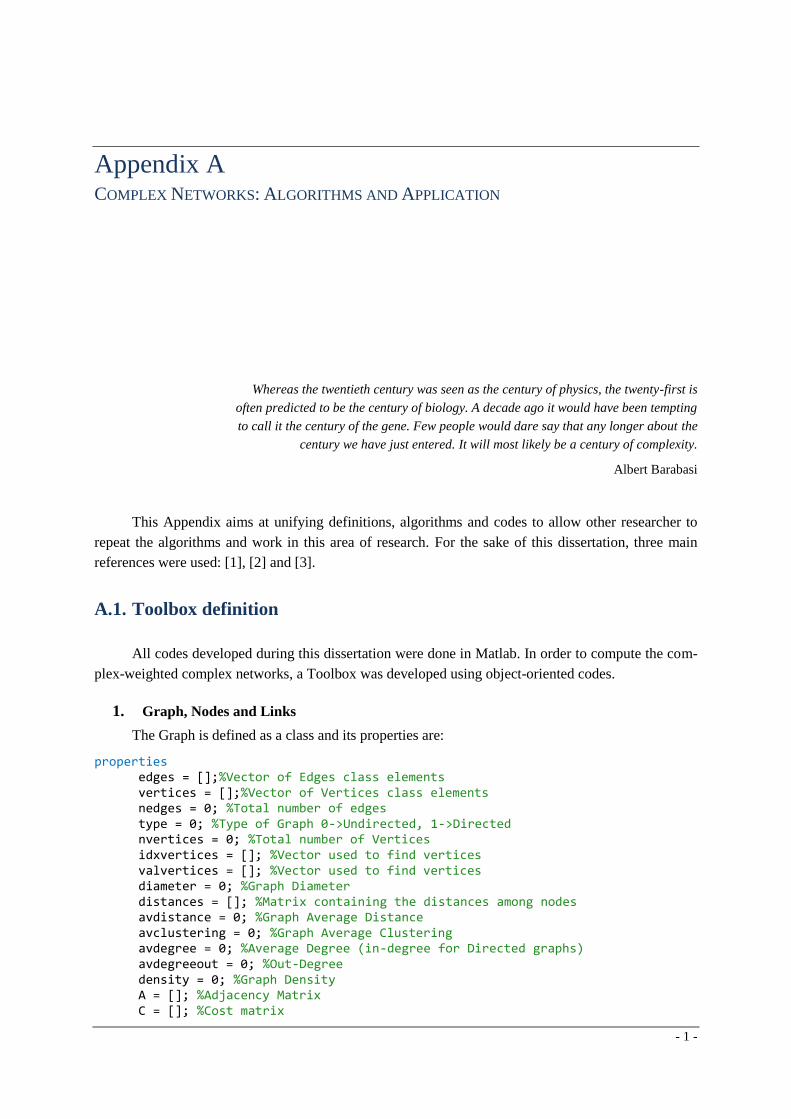
- 1 -
Appendix A
COMPLEX NETWORKS: ALGORITHMS AND APPLICATION
Whereas the twentieth century was seen as the century of physics, the twenty-first is
often predicted to be the century of biology. A decade ago it would have been tempting
to call it the century of the gene. Few people would dare say that any longer about the
century we have just entered. It will most likely be a century of complexity.
Albert Barabasi
This Appendix aims at unifying definitions, algorithms and codes to allow other researcher to repeat the algorithms and work in this area of research. For the sake of this dissertation, three main references were used: [1], [2] and [3].
A.1. Toolbox definition
All codes developed during this dissertation were done in Matlab. In order to compute the com-plex-weighted complex networks, a Toolbox was developed using object-oriented codes.
1. Graph, Nodes and Links
The Graph is defined as a class and its properties are:
properties edges = [];%Vector of Edges class elements vertices = [];%Vector of Vertices class elements nedges = 0; %Total number of edges type = 0; %Type of Graph 0->Undirected, 1->Directed nvertices = 0; %Total number of Vertices idxvertices = []; %Vector used to find vertices valvertices = []; %Vector used to find vertices diameter = 0; %Graph Diameter distances = []; %Matrix containing the distances among nodes avdistance = 0; %Graph Average Distance avclustering = 0; %Graph Average Clustering avdegree = 0; %Average Degree (in-degree for Directed graphs) avdegreeout = 0; %Out-Degree density = 0; %Graph Density A = []; %Adjacency Matrix C = []; %Cost matrix
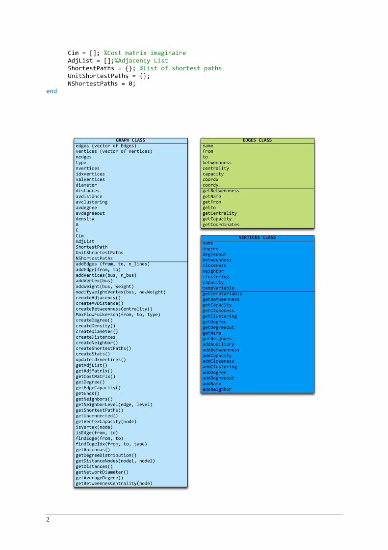
2
Cim = []; %Cost matrix imaginaire AdjList = [];%Adjacency List ShortestPaths = {}; %List of shortest paths UnitShortestPaths = {}; NShortestPaths = 0; end
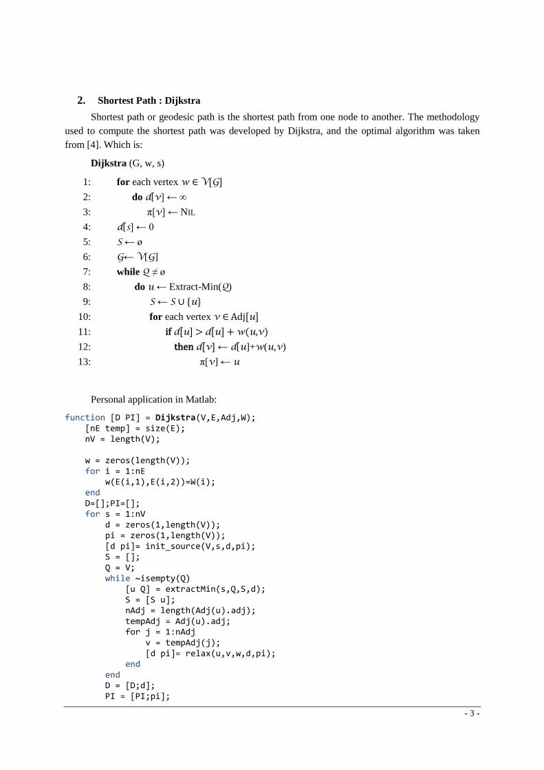
- 3 -
2. Shortest Path : Dijkstra
Shortest path or geodesic path is the shortest path from one node to another. The methodology used to compute the shortest path was developed by Dijkstra, and the optimal algorithm was taken from [4]. Which is:
Dijkstra (G, w, s)
1: for each vertex w ∈ V[G]
2: do d[v] ← ∞
3: π[v] ← NIL
4: d[s] ← 0
5: S ← ø
6: G← V[G]
7: while Q ≠ ø
8: do u ← Extract-Min(Q)
9: S ← S ∪ {u}
10: for each vertex v ∈ Adj[u]
11: if d[u] > d[u] + w(u,v)
12: then d[v] ← d[u]+w(u,v)
13: π[v] ← u
Personal application in Matlab:
function [D PI] = Dijkstra(V,E,Adj,W);
[nE temp] = size(E);
nV = length(V);
w = zeros(length(V));
for i = 1:nE
w(E(i,1),E(i,2))=W(i);
end
D=[];PI=[];
for s = 1:nV
d = zeros(1,length(V));
pi = zeros(1,length(V));
[d pi]= init_source(V,s,d,pi);
S = [];
Q = V;
while ~isempty(Q)
[u Q] = extractMin(s,Q,S,d);
S = [S u];
nAdj = length(Adj(u).adj);
tempAdj = Adj(u).adj;
for j = 1:nAdj
v = tempAdj(j);
[d pi]= relax(u,v,w,d,pi);
end
end
D = [D;d];
PI = [PI;pi];
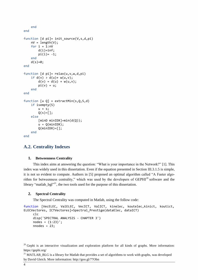
4
end
end
function [d pi]= init_source(V,s,d,pi)
nV = length(V);
for i = 1:nV
d(i)=inf;
pi(i)= -1;
end
d(s)=0;
end
function [d pi]= relax(u,v,w,d,pi)
if d(v) > d(u)+ w(u,v);
d(v) = d(u) + w(u,v);
pi(v) = u;
end
end
function [u Q] = extractMin(s,Q,S,d)
if isempty(S)
u = s;
Q(s)=[];
else
[minD minIDX]=min(d(Q));
u = Q(minIDX);
Q(minIDX)=[];
end
end
A.2. Centrality Indexes
1. Betweenness Centrality
This index aims at answering the question: “What is your importance in the Network?” [1]. This index was widely used in this dissertation. Even if the equation presented in Section III.3.1.5 is simple, it is not so evident to compute. Authors in [5] proposed an optimal algorithm called “A Faster algo-rithm for betweenness centrality,” which was used by the developers of GEPHI20 software and the library “matlab_bgl”21, the two tools used for the purpose of this dissertation.
2. Spectral Centrality
The Spectral Centrality was computed in Matlab, using the follow code:
function [VecELEC, ValELEC, VecICT, ValICT, kinelec, koutelec,kinict, koutict,
ELECVectores, ICTVectores]=Spectral_Prestige(dataElec, dataICT) clc disp('SPECTRAL ANALYSIS - CHAPTER 3') nodes = (1:23)'; nnodes = 23;
20 Gephi is an interactive visualization and exploration platform for all kinds of graphs. More information: https://gephi.org/ 21 MATLAB_BLG is a library for Matlab that provides a set of algorithms to work with graphs, was developed by David Gleich. More information: http://goo.gl/77Obn
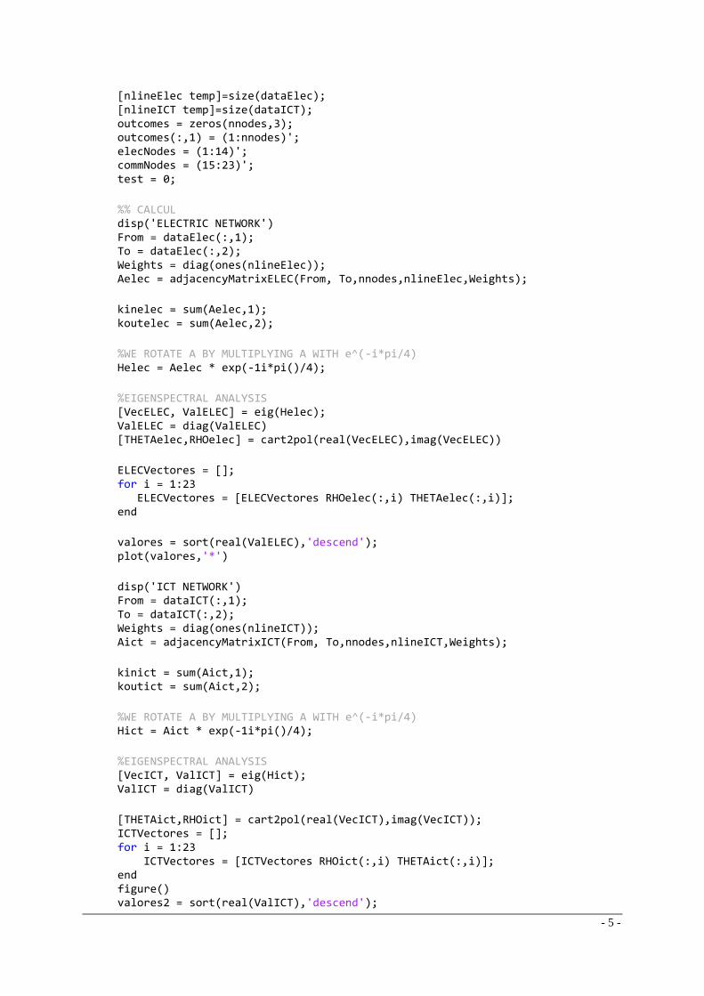
- 5 -
[nlineElec temp]=size(dataElec); [nlineICT temp]=size(dataICT); outcomes = zeros(nnodes,3); outcomes(:,1) = (1:nnodes)'; elecNodes = (1:14)'; commNodes = (15:23)'; test = 0;
%% CALCUL disp('ELECTRIC NETWORK') From = dataElec(:,1); To = dataElec(:,2); Weights = diag(ones(nlineElec)); Aelec = adjacencyMatrixELEC(From, To,nnodes,nlineElec,Weights);
kinelec = sum(Aelec,1); koutelec = sum(Aelec,2);
%WE ROTATE A BY MULTIPLYING A WITH e^(-i*pi/4) Helec = Aelec * exp(-1i*pi()/4);
%EIGENSPECTRAL ANALYSIS [VecELEC, ValELEC] = eig(Helec); ValELEC = diag(ValELEC) [THETAelec,RHOelec] = cart2pol(real(VecELEC),imag(VecELEC))
ELECVectores = []; for i = 1:23 ELECVectores = [ELECVectores RHOelec(:,i) THETAelec(:,i)]; end
valores = sort(real(ValELEC),'descend'); plot(valores,'*')
disp('ICT NETWORK') From = dataICT(:,1); To = dataICT(:,2); Weights = diag(ones(nlineICT)); Aict = adjacencyMatrixICT(From, To,nnodes,nlineICT,Weights);
kinict = sum(Aict,1); koutict = sum(Aict,2);
%WE ROTATE A BY MULTIPLYING A WITH e^(-i*pi/4) Hict = Aict * exp(-1i*pi()/4);
%EIGENSPECTRAL ANALYSIS [VecICT, ValICT] = eig(Hict); ValICT = diag(ValICT)
[THETAict,RHOict] = cart2pol(real(VecICT),imag(VecICT)); ICTVectores = []; for i = 1:23 ICTVectores = [ICTVectores RHOict(:,i) THETAict(:,i)]; end figure() valores2 = sort(real(ValICT),'descend');
6
plot(valores2,'*')
res1 = [ValELEC';VecELEC]; res2 = [ValICT';VecICT];
end
function A = adjacencyMatrixELEC(From, To,nnodes,nline,Weights) A = zeros(nnodes); for i = 1:nline A(From(i),To(i))=A(From(i),To(i))+Weights(i); A(To(i),From(i))=A(To(i),From(i))+(Weights(i)*1i); end
end function A = adjacencyMatrixICT(From, To,nnodes,nline,Weights)
A = zeros(nnodes); for i = 1:nline A(From(i),To(i))=A(From(i),To(i))+Weights(i)+(Weights(i)*1i); A(To(i),From(i))=A(To(i),From(i))+Weights(i)+(Weights(i)*1i); end
end
A.3. More information
Many more information about small-world [6], scale-free networks [7] can be found in the lit-erature. This information is important, since it allows knowing other properties of complex systems, about their structure and topology. M. Newman published a Survey con Complex Systems [8], which emphasizes the papers with the highest impact in this subject.
A.4. Bibliography
[1] Reuven Cohen and Shlomo Havlin, Complex Networks: Structure, Robustness and Func-
tion, Cambridge University Press, 2010. [2] Mark Newman, “The Structure and function of Complex Networks,” SIAM Review, Vol.
45, No. 2, pp. 167-256, 2003. [3] S. Boccaletti, V. Latora, Y. Moreno, M. Chavez, and D.-U. Hwang, “Complex Networks:
Structure and Dynamics,” Physics Reports, N. 424, pp. 175-308, 2006. [4] Thomas Cormen, Charles Leiserson, Ronald Rivest and Clifford Stein, Introduction to Al-
gorithms, Cambridge: The MIT Press, 2nd Edition, 2001. [5] Ulrik Brandes, “A Faster algorithm for Betweenness Centrality,” Journal of Mathematical
Sociology, Vol. 25, N. 2, pp. 163-177, 2001. [6] Xiao Fan Wang and Guanrong Chen, “Complex Networks: Small-world, Scale-Free and
beyond,” IEEE Circuits and Systems Magazine, pp. 6-20, First quarter 2003. [7] Albert-Lázló Barabási and Enric Bonabeau, “Scale-free Networks,” Scientific American, pp.
50-59. 2003. [8] Mark Newman, “Complex Systems: A survey,” American Journal of Physics, Vol 79, pp.
800-810, 2011.
- 7 -
Appendix B
RECENT ATTACKS AND ICTS FAILURES
Quis custodied ipsos custodies
Decimus lunius luvenalis
Every day it is likely to find sensationalist headlines as: “.S. Power and water utilities face daily cyber-attacks” (in Homeland Security News Wire, Published on 6 April 2012), “Russia says many states arming for cyber warfare” (in Reuters, Published on 25 April 2012), “Hacker could take over traffic and rail-road control systems using back-door” (in Magazine “Info-Security,” Published on 26 April 2012). But, does this news show a reality or just a paranoia state? This appendix summarizes the main and recent attacks to Power System facilities worldwide, as well as, some failures on information and communication systems that have been remembered as historical events due to their great impact on the life of hundreds of citizens.
B.1. Recent Attacks against industrial control systems
1. Flame – 2012
Flame malware (also known as Flamer or sKyWIper) was discovered in 2012 by the MAHER Center of Iranian National Computer Emergency Response Team (CERT) [1], Karspersky Lab [2] and CrySyS [3]. The origin of this malware is unknown, but it has been used for targeted cyber espionage in Middle Eastern countries.
This malware attacks computers running the Microsoft Windows operating system (including Windows XP, Vista and 7), and its main objective is to impact on SCADA Security Systems [4]. It performs network sniffing, collects a list of vulnerable passwords, transfers saved data on control servers, and it has the ability to record audio, screen-shots, keyboard activity and network traffic. It is transferred over a local network (LAN) via USB stick or via file sharing.
2. Worm W32.Duqu – 2011
On 1st September 2011, the computer worm Duqu was discovered by the Laboratory of Cryp-tography and System Security (CrySys) in Hungary. According to the U.S. Department of Homeland, the Worm Duqu is an information-gathering threat that targeted specific organizations, including in-dustrial control systems (ICSs) manufacturers [5]. According to the reports, the code appears to look

8
for information such as design documents that could be used to launch a future attack against a facility under the control of an ICS -including electric generation, water/wastewaters treatment, oil and gas production/distribution/refining, chemical/petrochemical processing, transportation systems, and building automation systems.
3. Stuxnet – 2010
It is a computer sophisticated worm discovered in July 2010 in Iran [6] and has been recognized as one of the most complex threat ever found. It was primarily written to target industrial control sys-tems which have the Siemens SIMATIC WinCC/Step 7 controller software installed, and its final goal was to reprogram industrial control systems (ICS) by modifying the code on programmable logic con-trollers (PLCs) to make them work in a very specific manner, the attacker intended to hide those changes from the operator of the equipment. Most of the victims were located in Iran, Indonesia, and India, it was reported 14 power plants infected (among them the Bushehr Nuclear Power plant in Iran) and more than 50000 Windows computers. However, there is no record of mortal consequences.
The worm exploited unknown windows vulnerabilities that allowed it to spread from computer to computer via USB stick and thus infect computers and networks that are not normally connected to the Internet. It had two specific characteristics, it get more complex over time (it has four zero-day exploits) and it has a deadline on 24th June 2012, date when it will stop spreading and delete itself [7], [8]. According to several publications, USA and Israel are the most common suspects, however it re-mains highly speculative and it will remain a mystery [9], [10]. Authors in [11] study how Stuxnet infects and propagates using a typical (but hypothetical) security model.
4. The Night Dragon – 2009
Since November 2009, hackers have stolen confidential data to companies from the energy sec-tor in the United States, this series of attacks was called “The Night Dragon” since it was originated from several locations in China [12].
This coordinated attack was conducted against global oil, energy and petrochemical companies, and against individual and executives of such enterprises. Each attack was divided into five steps, ac-cording to McAffe:
1. Attack through SQL-injection on extranet web servers to allow remote command execution. 2. Gained access to sensitive internal desktops and servers. 3. Accessed additional usernames and passwords. 4. Enabled direct communication from infected machines to the Internet. 5. Exfiltrated email archives and other highly sensitive documents.
Attackers used a “mix of hacking techniques” including SQL-injection and spear-phishing that compromised corporate VNP accounts. Despite this kind of attacks are common in Computer Net-works; it is the first time this kind of attacks was focused against the Energy Sector [13].
5. Daimler-Chrysler plants - Zotob Worm – 2005
In August 2005, 13 assembly lines of Daimler-Chrysler US auto manufacturing plants (located at Illinois, Indiana, Wisconsin, Ohio, Delaware and Michigan) went offline for almost one hour due to several PC outages caused by the infection of Zotob, RBot and IRCBot worms. These viruses exploit-ed a hole in the PnP (Plug-and-play) of computers running Windows 2000 [14]. The estimated cost impact was US$14 million [15].
- 9 -
6. Ohio Davis-Besse Nuclear Plant – 2003
On January 25, 2003 the worm MS SQL Server 2000 attacked several computers in the Ohio Davis-Besse Nuclear plant. This computer blackout caused data overload in the site network and therefore the computers were unable to communicate with each other. Fortunately the plant control and protection functions were not affected [16]. However, the safety monitoring system was offline for 5 hours.
Even if the plant network is well protected by a firewall, the worm by-passed the access controls through a T1 Connection line used by a consultant.
7. Nimda worm – 2001
The Nimda worm, widely spread in the world in 2001, reached in September 2001 the internal network of a major EMS/SCADA vendor and then attacked the EMS/SCADA networks of all its cus-tomers via the support network [17].
This worm affected mainly system running Microsoft Windows 95/98, ME, NT and 2000 and propagated through email arriving as a multipart/alternative message. In the host computer, the Nimda worm caused denial-of-service conditions on networks affecting the internal network [18].
8. Code Red II Worm – 2001
Code Red II Worm was released on August 4 2001, this worm created a back-door to allow at-tacks on vulnerable systems. It exploited a security hole in Microsoft web server software. This worm affected the internal network of a company that provides services to numerous electric utility compa-nies. Although the infected networks were protected and not exposed to the Internet, the worm used the private frame relay network connected to the service company [18].
9. Australian Sewage System – 2000
On February-April 2000, Vitek Boden realized a series of electronic attack on the sewage con-trol system in Queensland – Australia, causing millions of liters of raw sewage to spill out into local parks and rivers [19]. He is an expert on SCADA systems and radio-controlled sewage equipment, and at that time he was applying for a job at the sewage control system, but his application was rejected, the reason why he revenged against the enterprise.
In the Australian Sewage System, each pumping station is able to receive commands from a Control Center by means of dedicated analog two-way radio system, using different frequencies. Vitek Boden installed some of these communication systems at the Australian Sewage System and the day he was captured in his car, police found in his laptop specialized software for accessing and control-ling sewage management systems, as well as radio-equipment compatible with those used at the sew-age system [20].
At the control center, engineers recognized that they were under attack after the detection of an increased radio traffic, that pumps were not responding under demand, some alarms were not reporting to the control center and the loss of communication between the control center and several pumping stations [21].
This attack demonstrated that intentional and targeted attacks by a knowledgeable person are re-al and may be catastrophic. As well, that this was just one attack by one person against a single sys-tem, therefore terrorist or even enemy nations can attack vulnerable infrastructures easily and in a much higher scale.
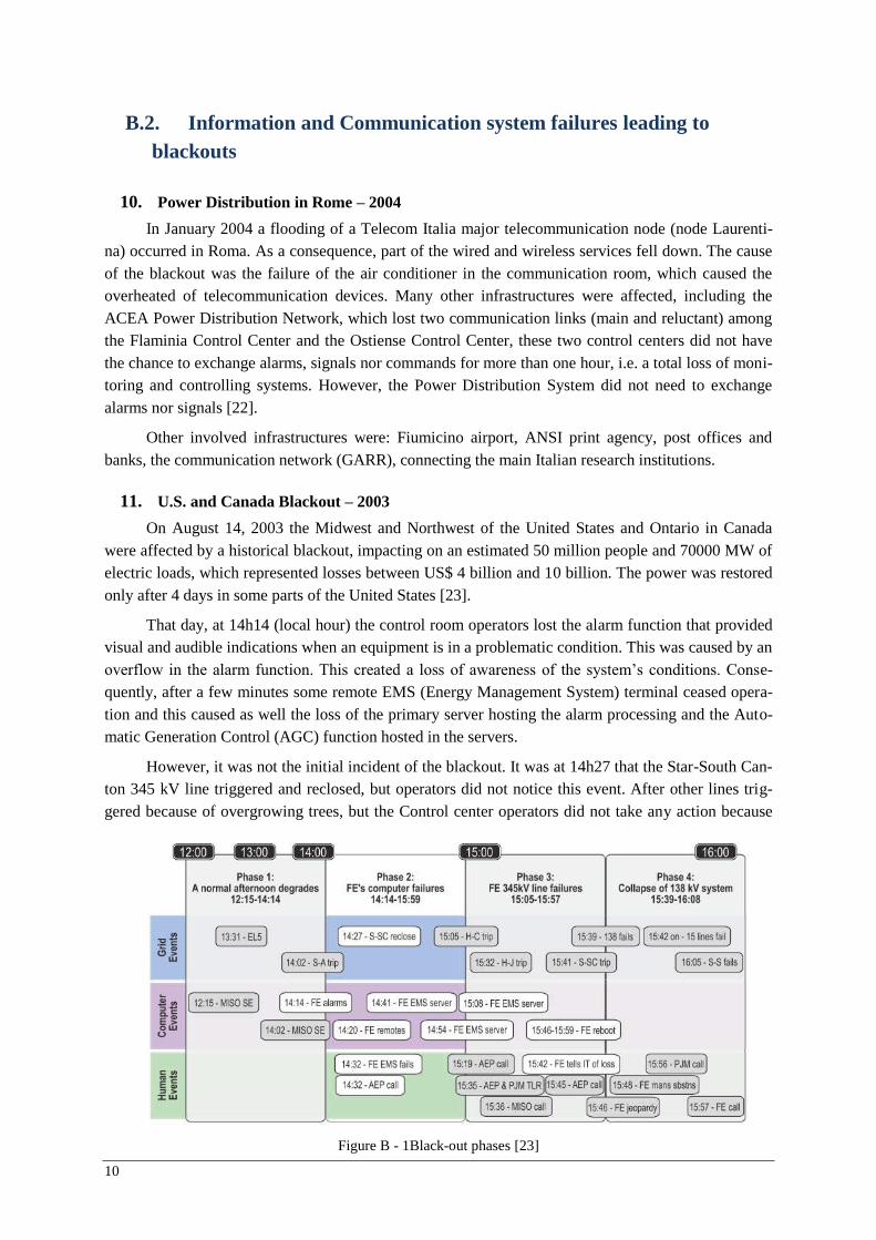
10
B.2. Information and Communication system failures leading to blackouts
10. Power Distribution in Rome – 2004
In January 2004 a flooding of a Telecom Italia major telecommunication node (node Laurenti-na) occurred in Roma. As a consequence, part of the wired and wireless services fell down. The cause of the blackout was the failure of the air conditioner in the communication room, which caused the overheated of telecommunication devices. Many other infrastructures were affected, including the ACEA Power Distribution Network, which lost two communication links (main and reluctant) among the Flaminia Control Center and the Ostiense Control Center, these two control centers did not have the chance to exchange alarms, signals nor commands for more than one hour, i.e. a total loss of moni-toring and controlling systems. However, the Power Distribution System did not need to exchange alarms nor signals [22].
Other involved infrastructures were: Fiumicino airport, ANSI print agency, post offices and banks, the communication network (GARR), connecting the main Italian research institutions.
11. U.S. and Canada Blackout – 2003
On August 14, 2003 the Midwest and Northwest of the United States and Ontario in Canada were affected by a historical blackout, impacting on an estimated 50 million people and 70000 MW of electric loads, which represented losses between US$ 4 billion and 10 billion. The power was restored only after 4 days in some parts of the United States [23].
That day, at 14h14 (local hour) the control room operators lost the alarm function that provided visual and audible indications when an equipment is in a problematic condition. This was caused by an overflow in the alarm function. This created a loss of awareness of the system’s conditions. Conse-quently, after a few minutes some remote EMS (Energy Management System) terminal ceased opera-tion and this caused as well the loss of the primary server hosting the alarm processing and the Auto-matic Generation Control (AGC) function hosted in the servers.
However, it was not the initial incident of the blackout. It was at 14h27 that the Star-South Can-ton 345 kV line triggered and reclosed, but operators did not notice this event. After other lines trig-gered because of overgrowing trees, but the Control center operators did not take any action because
Figure B - 1Black-out phases [23]

- 11 -
they did not realize these events caused by the lack of alarms. This caused a cascade effect on many lines. It is important to mention that the control center lacked of alarm failure detection systems.
This blackout had a negative impact on the cellular communication network since at the backup power at the cellular sites the generators ran out of fuel.
Figure B - 1 presents the time line of the main phases of the Blackout. This figure shows that the blackout was originated by a combination of errors and failures in the power grid, the ICT network and the human behavior.
More information can be found in [24], [25] and [26].
12. Ertan Hydro Station – 2000
On October 13 2000, the control system of ERTAN hydro station in China received unexpected signals that almost cause the collapse of the Sichuan Power System [27].
13. Hydro-Quebec – 1988
A remote load-shedding system failed to operate due to a communication system's failure in the control center, which led to a sequence of line trips followed by line overloading, tripping of generat-ing units, and the loss of dc interconnections.
B.3. Conclusions
Recent events reveal several facts:
Failures in ICT infrastructure can actually affect Power Systems.
There is a tendency to perform targeted cyber and physical attacks, and these advanced threats now can target people as well through social engineering, using fake emails and oth-er manipulation methods. Therefore, it is needed to improve the users’ education and awareness to succeed against external targeted threats.
Isolation from the internet is not an effective defense and all power systems that are con-trolled by software are vulnerable to cyber threats because internal networks can be attacked via usb keys or service networks.
Terrorists and war fighters recognized that it is more effective to attack ICT infrastructures directly, than to physically attack their targets.
B.4. Bibliography
[1] MAHER Computer Emergency Response Team Coordination Center, “Identification of a New Targeted Cyber-Attack,” ID: IRCEN2012051505, May 28, 2012. [Online]: Available: http://www.certcc.ir
[2] Karpesky Lab, “Ne investiagion points to three new Flame-related malicious programs: at least one still in the wild,” 17 September 2012. [Online]: Available: http://www.karspesky.com
[3] CrySyS Lab Laboratory of Cryptography and System Security, “A complex malware for targeted attacks,” Budapest: May 31, 2012.
12
[4] Eric Byres, “Flame Malware and SCADA Security: What are the impacts?” May 29, 2012. [Online]: Available: http://www.tofinosecurity.com
[5] US Department of Homeland Security, “ICS-CERT Alert W32.DUQU: An information-Gathering Malware Targeting Industrial Control Systems Manufacturers,” October 2011.
[6] Nicolas Faillere, Liam Murchu and Eric Chien, “W.32 Stuxnet Dossier,” Symantec, Febru-ary 2011. V. 1.4.
[7] T.M. Chen and S. Abu-Nimeh, “Lessons from Stuxtnet,” Computer. Vol. 44, no. 4, pp. 91-93, April 2011.
[8] Ralph Lagner, “Stuxnet: Dissecting a cyberwarfare weapon,” IEEE Security Privacy. Vol. 9, No. 3, pp. 49-51, 2011.
[9] Robert McMillan, “Siemens: Stuxnet worm hit industrial systems,” Computer World, Sep-tember 14, 2010, [Online] Available: http://www.computerworld.com
[10] Bruce Schneier, “The story behind the Stuxnet virus,” FORBES, July 10, 2010. [Online] Available: http://www.forbes.com
[11] Eric Byres, Andrew Ginter and Joel Langil, “How Stuxnet spreads – A study on infection paths in best practice systems,” Tofino Security, Februari 22, 2011. [Online] Available: http://abterra.ca
[12] McAfee, “Global Energy Cyberattacks: Night Dragon,” White Paper. Feb 10, 2011. [13] Fraser Howard, “Night Dragon attacks: myth or reality?” Naked Security, Feb. 11, 2011.
[Online] Available: http://nakedsecurity.sophos.com [14] Paul Roberts, “Zotob, PnP Worms Slam 13 DaimlerChrysler Plan,” EWEEK, August
2005. [Online] Available: http://www.eweek.com [15] Tofino Security, “Case Profile: Daimler Crysler,” Cyber Security Incident CP-104, Ver-
sion 1. [Online] Available: http://www.tofinosecurity.com [16] US. Nuclear Regulatory commission Office of Nuclear Reactor Regulation, “Potential
Vulnerability of Plant computer network to worm infection,” NRC Information Notice 2003-14. Washington, D.C: August 2003.
[17] CERT, “CERT advisory CA-2001-26 Nimda Worm,” September 25; 2001. [Online] Available: http://www.cert.org/advisories/CA-2001-26.html
[18] NERC North American Electric Reliability Council, “Urgent Action Standard 1200 – Cyber security,” Princeton: August 2003.
[19] Smith Tony, “Hacker jailed for revenge sewage attacks,” The Register, October 31, 2012. [Online] Available: http://www.theregister.co.uk
[20] Marshal Abrams and Joe Weiss, “Malicious Control System Cyber Security attack case study – Maroochy Water Services, Australia,” The MITRE Corporation, 2008. [Online] Available: http://csrc.nist.gov
[21] Jill Slay and Michael Miller, “Lessons Learned from the Marrochy Water Breach,” Criti-cal Infrastructure Protection, Ch. 6, Vol. 253, pp. 73-82, Springer US, 2007.
[22] Tools and Techniques for Interdependency analysis. June 2007, pp. 45-51 [Online]: Available: http://www.irriis.org, EU Project IRRIIS, deliverable D222.
[23] US. - Canada Power System outage task force, “Final Report on the August 14, 2003 Blackout in the United States and Canada: Causes and Recommendations,” 2004.
[24] New York Independent System Operator, “Interim report on August 14, 2003 Blackout,” April, 2004.
[25] New York Independent System Operator, “Blackout august 14, 2003,” February 2005. [26] NERC North American Electric Reliability Council, “Technical analysis of the August
14, 2003: What happened, why and what did we learn?” July 2004.

- 13 -
[27] CRUTIAL Project, “Methodologies Synthesis,” Delivrable 3, 31 December 2006.

- 15 -
APPENDIX C
PROJECTS INCLUDING COUPLED INFRASTRUCTURES
We may brave human laws, but we cannot resist natural ones
Jules Verne
This appendix summarizes several projects that have worked on Critical Infrastructures analy-sis, including modeling and simulation. As well, some of the standards that present guidelines to build these complexes coupled systems.
C.1. Projects
1. SINARI Project
Name: Sécurité des Infrastructures et Analyse de Risques
Website: http://www.sinari.org
Dates: 2010 - 2013
Project type: French - ANR
Originalities: Creation of a test platform that integrates power system emulation, communica-tion network and SCADA simulation and real automatisms.
Objectives: The SINARI Project objectives are: to identify the hazards and risks inherent in in-tegrated infrastructures, to develop necessary ICT defenses, to test the most representative of these defenses and finally to evaluate their effectiveness [1]-[2].
2. SEESGEN-ICT
Name: Supporting Energy Efficiency in Smart GENeration grids through ICT”
Website: http://seesgen-ict.rse-web.it
Dates: 2009 - 2011
Project type: European
Originalities: Proposition of policy recommendations for the introduction of ICT into the smart distributed power generation grids.
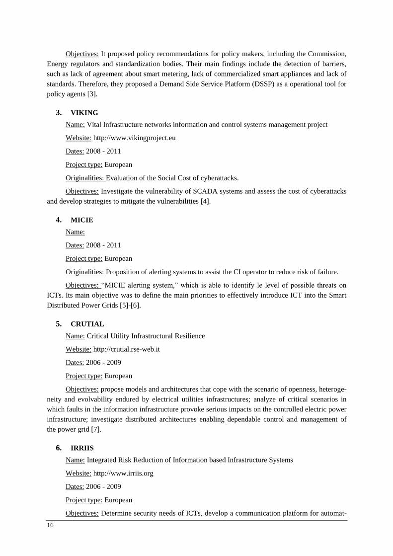
16
Objectives: It proposed policy recommendations for policy makers, including the Commission, Energy regulators and standardization bodies. Their main findings include the detection of barriers, such as lack of agreement about smart metering, lack of commercialized smart appliances and lack of standards. Therefore, they proposed a Demand Side Service Platform (DSSP) as a operational tool for policy agents [3].
3. VIKING
Name: Vital Infrastructure networks information and control systems management project
Website: http://www.vikingproject.eu
Dates: 2008 - 2011
Project type: European
Originalities: Evaluation of the Social Cost of cyberattacks.
Objectives: Investigate the vulnerability of SCADA systems and assess the cost of cyberattacks and develop strategies to mitigate the vulnerabilities [4].
4. MICIE
Name:
Dates: 2008 - 2011
Project type: European
Originalities: Proposition of alerting systems to assist the CI operator to reduce risk of failure.
Objectives: “MICIE alerting system,” which is able to identify le level of possible threats on ICTs. Its main objective was to define the main priorities to effectively introduce ICT into the Smart Distributed Power Grids [5]-[6].
5. CRUTIAL
Name: Critical Utility Infrastructural Resilience
Website: http://crutial.rse-web.it
Dates: 2006 - 2009
Project type: European
Objectives: propose models and architectures that cope with the scenario of openness, heteroge-neity and evolvability endured by electrical utilities infrastructures; analyze of critical scenarios in which faults in the information infrastructure provoke serious impacts on the controlled electric power infrastructure; investigate distributed architectures enabling dependable control and management of the power grid [7].
6. IRRIIS
Name: Integrated Risk Reduction of Information based Infrastructure Systems
Website: http://www.irriis.org
Dates: 2006 - 2009
Project type: European
Objectives: Determine security needs of ICTs, develop a communication platform for automat-
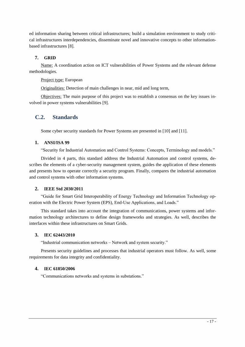
- 17 -
ed information sharing between critical infrastructures; build a simulation environment to study criti-cal infrastructures interdependencies, disseminate novel and innovative concepts to other information-based infrastructures [8].
7. GRID
Name: A coordination action on ICT vulnerabilities of Power Systems and the relevant defense methodologies.
Project type: European
Originalities: Detection of main challenges in near, mid and long term,
Objectives: The main purpose of this project was to establish a consensus on the key issues in-volved in power systems vulnerabilities [9].
C.2. Standards
Some cyber security standards for Power Systems are presented in [10] and [11].
1. ANSI/ISA 99
“Security for Industrial Automation and Control Systems: Concepts, Terminology and models.”
Divided in 4 parts, this standard address the Industrial Automation and control systems, de-scribes the elements of a cyber-security management system, guides the application of these elements and presents how to operate correctly a security program. Finally, compares the industrial automation and control systems with other information systems.
2. IEEE Std 2030/2011
“Guide for Smart Grid Interoperability of Energy Technology and Information Technology op-eration with the Electric Power System (EPS), End-Use Applications, and Loads.”
This standard takes into account the integration of communications, power systems and infor-mation technology architectures to define design frameworks and strategies. As well, describes the interfaces within these infrastructures on Smart Grids.
3. IEC 62443/2010
“Industrial communication networks – Network and system security.”
Presents security guidelines and processes that industrial operators must follow. As well, some requirements for data integrity and confidentiality.
4. IEC 61850/2006
“Communications networks and systems in substations.”
18
Standard IEC 61850 was created because before its application, specific proprietary communi-cation protocols were developed by each manufacturer, this caused the need of complicated and ex-pensive protocol converters in order to use IEDs from different vendors. Therefore, this standard was designed to unify and provide a single protocol for a complete substation, to facilitate object modeling of data requirement in the substation, to define the basic services required to transfer data using differ-ent communication protocols and to allow the interoperability between IEDs from different vendors [12]. This Standard is divided into 10 parts:
5. IEEE Std 1686/2007
“IEEE Standard for Substation Intelligent Electronic Devices (IEDs) Cyber Security Capabili-ties.”
Describes the requirements for Substation Intelligent Electronic Devices to secure the lo-cal/remote access and thus secure the substation. As well, it proposes features to develop a defensive procedure.
6. Mandate 490 - 2011
“Standardization Mandate to European Standardisation Organisations to support European Smart Grid Deployment.”
The main objective of this mandate is to develop and/or update standards that deal with the in-tegration of Information and Communication Technologies on Smart Grids.
C.3. Bibliography
[1] J. McDonald, et al, “The SINARI Project Security: Security Analysis and Risk Assessment applied to the electrical Distribution Network.” CIRED Conference. Stockholm, 2013.
[2] R. Caire, J. Sanchez and N. Hadjsaid, “Vulnerability assessment of coupled heterogeneous critical infrastructures: a Co-Simulation approach with a test bed validation,” IEEE PES In-
novative Smart Grid Technologies, Europe 2013, Copenhagen, 2013. [3] G. Franchioni, “SEESGEN-ICT: Presentation of the results,” Presentation slides, July 2011. [4] VIKING Consortium, Summary of VIKING Results, 2011. [5] MICIE Project, Deliverable D 2.2.3 – Interdependency modeling framework, indicators and
models – final report. Dec. 31st 2010.
Part 1 Introduction and overview
Part 2 Glossary
Part 3 General requirements
Part 4 System and project management
Part 5 Communication requirements for functions and device models
Part 6 Configuration description language for communication in electrical substations related IEDs
Part 7 1. Principles and Models, 2. Abstract communication service interface, 3. Common data classes, 4. compatible logical node (LN) classes and data classes
Part 8 Mapping to MMS and to ISO/IEC 8802-3
Part 9 Sampled values over serial unidirectional multidrop point-to-point link and ISO 8802-3
Part 10 Conformance testing
- 19 -
[6] MICIE Project, Project final report, 2011. [7] CRUTIAL Project, Methodologies Synthesis, Deliverable 3, Dec 31st 2006. [8] IRRIIS Project, Autonome Intelligent System. Deliverable D 4.4.5, Fraunhofer Flentge,
2006. [9] N. Hadjsaid, Securing Critical Infrastructures: The power and ICT perspective, Presenta-
tion slides. [10] M. Masera, “ICT aspects of power systems and their security” JCR Scientific and Tech-
nical Report, Luxembourg: JRC European Commission, 2011. [11] L. Pietre-Cambacedes, T. Kropp, J. Weiss and R. Pellizzoni, “Cybersecurity standards for
the electric power industry – a “Survival kit”,” 2008 Cigré Session, Study committee D2 “Information, Telecommunication and Telecontrol systems in the electric power industries”, 2008.
[12] ABB. ABB Review Special Report IEC 61850. Zürich: ABB Group R&D and Technolo-gy, 2010.

- 21 -
APPENDIX D
PUBLICATIONS
Our virtues and our failings are inseparable,
like force and matter. When they separate, man is no more.
Nikola Tesla
This appendix summarizes the publications arising from this thesis:
International Journals:
[1] A. Merdassi, R. Caire, N. Hadjsaid, J.L. Sanchez, M. Kellil, N. Oualha, S. Machenaud, D. Georges, C. Bousba, N. Vignol, P. Carer, J. McDonald, "Modeling methods coupled electrical networks and ICT. An inventory" EJEE 2012, VOL 15/6, pp.557-585.
Conferences:
[2] J. L. Sánchez, R. Caire and N. Hadjsaid. "ICT and Electric Power Systems Interde-pendencies Modeling," ETG-CRIS Conference, Berlin - Germany, 5-6 November 2013. Also, published at the ETG-Association Magazine, July 2014.
[3] J. L. Sánchez, R. Caire and N. Hadjsaid. "Application of Hermitian Adjacency Matri-ces for the Vulnerability Analysis of Power Systems," IEEE PES ISGT Europe 2013, Copenhagen - Denmark.
[4] R. Caire, J. L. Sánchez and N. Hadjsaid. "Vulnerability Analysis of Coupled Hetero-geneous Critical Infrastructures: a Co-simulation Approach with a Testbed Validation," IEEE PES ISGT Europe 2013, Copenhagen - Denmark [Invited paper].
[5] J. McDonald, H. Decroix, R. Caire, J.L. Sánchez, S. Chollet, N. Oualha, A. Puccetti, A. Hecker, C. Chaudet, H. Piat, D. Georges, F. Planchon, “The SINARI Project Securi-ty Analysis and Risk assessment applied to the Electrical Distribution Network,” 22nd International Conference on Electricity Distribution CIRED, 10-13 June 2013, Stock-holm – Sweden.
[6] J. L. Sánchez, R. Caire and N. Hadjsaid. "ICT and Power Distribution Modeling using Complex Networks," IEEE Powertech Conference, Grenoble - France, 16-20 June 2013.

22
Workshops without proceedings:
[7] J. L. Sánchez, R. Caire and N. Hadjsaid. "Towards a Complex Networks Modeling of Interdependent Critical Infrastructures." WISG January 2013, Troyes - France.
[8] H. Piat, D. Georges, A. Petrequin, N. Oualha, L. Correnson, N. Vignol, J. Mcdonald, F. Colin, F. PLanchon, T. Braconnier, F. Costa, R. Caire, J. L. Sánchez, A. Labonne, A. Hecker, "Implementation of Interdependent Critical Infrastructures for Electricity Sup-ply." WISG January 2013, Troyes - France.
[9] A. Merdassi, R. Caire, N. Hadjsaid, J. L. Sánchez, M. Viziteu, M. Kellil, N. Oualha, S. Machenaud, D. Georges, C. Bousba, N. Vignol, P. Carer, J. McDonald, L. P. Cambacé-dès, C. Claude, A. Hecker, "Etat de l’art sur les méthodes de modélisation pour les in-frastructures critiques interdépendantes". WISG January 2011, Troyes - France.
Many others will come, to find recent publications, please visit my website at:
http://www.josesancheztorres.com/publications
VULNERABILITE , INTERDEPENDANCE ET ANALYSE DES RISQUES DES POSTES SOURCES ET
DES MODES D’EXPLOITATION DECENTRALISES DES RESEAUX ELECTRIQUES
Résumé ─ Au vu de l’utilisation croissante des technologies de l’information et de la communication dans les réseaux électriques, il est indispensable d’étudier l’étroite liaison entre ces infrastructures et d’avoir une vision intégrée du système couplé. Cette thèse porte ainsi sur la modélisation des systèmes multi-infrastructures. Cela inclut les interdépendances et les trajectoires de défaillances de type modes communs, aggravations et cascades. Il est en effet nécessaire d’identifier les points de faiblesse qui peuvent déclencher une ou de multiples défaillance(s), se succéder en cascade au travers de ces infrastructures liées et ainsi entrainer des défaillances inattendues et de plus en plus graves dans des autres infrastructures. Dans cette optique, différents modèles basés sur la théorie des Réseaux Complexes sont développés afin d’identifier les composants les plus importantes, et pourtant critiques, dans le système interconnecté. Un des principaux verrous scientifiques levé dans cette thèse est relatif au dé-veloppement d'un modèle mathématique « unifié » afin de représenter les comportements des multiples infrastructures non-homogènes qui ont des interdépendances asymétriques. Mots clés : Infrastructures critiques, Interdépendances, Réseau électrique, Réseau de communication, Réseaux complexes, Systèmes couplés, Technologies de l’information et de la communication, Vulné-rabilités.
VULNERABILITY , INTERDEPENDENCIES AND RISK ANALYSIS OF COUPLED INFRASTRUCTURES: POWER DISTRIBUTION NETWORK AND ICT
Abstract ─ In view of the increasing use of Information and Communication Technol-
ogies in power systems, it is essential to study the interdependencies between these coupled heterogeneous systems. This thesis focuses on the modeling of multi- infrastructure systems. This includes interdependencies and the three major failures families: common mode, escalat-ing and cascading. It is indeed necessary to identify the weaknesses that can trigger one or multiple failure(s) and cascade through these interdependent infrastructures, causing unex-pected and increasingly more serious failures to other infrastructures. In this context, different approaches, based on the theory of Complex Networks, are developed to identify the most critical components in the coupled heterogeneous system. One of the major scientific barriers addressed in this thesis is the development of a unified mathematical model to represent the behavior of multiple heterogeneous systems with complex asymmetrical communication pat-terns. Keywords: Critical infrastructures, Interdependence, Power grid, Secure operation, Vulnerability.
Laboratoire de Génie Electrique de Grenoble – G2ELAB Grenoble INP / UJF / CNR / Université de Grenoble
11 rue des mathématiques BP 46
38402, St. Martin d’Hères CEDEX FRANCE