WP/07/172

Volatility and Jump Risk Premia in Emerging Market Bonds

John M. Matovu

© 2007 International Monetary Fund WP/07/172 IMF Working Paper Middle East and Central Asia Department

Volatility and Jump Risk Premia in Emerging Market Bonds

Prepared by John M. Matovu1

Authorized for distribution by Aasim M. Husain

July 2007

Abstract

This Working Paper should not be reported as representing the views of the IMF. The views expressed in this Working Paper are those of the author(s) and do not necessarily represent those of the IMF or IMF policy. Working Papers describe research in progress by the author(s) and are published to elicit comments and to further debate.

There is strong evidence that interest rates and bond yield movements exhibit both stochastic volatility and unanticipated jumps. The presence of frequent jumps makes it natural to ask whether there is a premium for jump risk embedded in observed bond yields. This paper identifies a class of jump-diffusion models that are successful in approximating the term structure of interest rates of emerging markets. The parameters of the term structure of interest rates are reconciled with the associated bond yields by estimating the volatility and jump risk premia in highly volatile markets. Using the simulated method of moments (SMM), results suggest that all variants of models which do not take into account stochastic volatility and unanticipated jumps cannot generate the non-normalities consistent with the observed interest rates. Jumps occur (8,10) times a year in Argentina and Brazil, respectively. The size and variance of these jumps is also of statistical significance. JEL Classification Numbers: G13, G15

Keywords: Volatility, Jumps and Risk Premia

Author’s E-Mail Address: jmatovu@imf.org

1 I would like to thank Aasim Husain and several other colleagues at the Fund who provided useful comments, suggestions, and insights that helped enhance the quality of this paper.

2

Contents Page

I. Introduction ............................................................................................................................3

II. Model Specification ..............................................................................................................5

III. Econometric Approach ........................................................................................................7

IV. Data Sources ........................................................................................................................8

V. Empirical Results ..................................................................................................................9 A. SNP Model for Interest Rates ...................................................................................9 B. Simple Model with Constant Volatility (CIR) ........................................................10 C. Model with Stochastic Volatility (SV)....................................................................11 D. Model with Varying Volatility and Jumps (SVJ) ...................................................11 E. Volatility and Jump Risk Premia.............................................................................12

VI. Conclusion .........................................................................................................................13

Appendix 1. SNP Auxilliary Model .........................................................................................................14

References................................................................................................................................16

Tables 1. SNP Density Estimation ......................................................................................................19 2. EMM Estimates of the Jump Diffusion Stochastic Model for Argentina............................20 3. EMM Estimates of the Jump Diffusion Stochastic Model for Brazil ..................................21 4. Volatility and Jump Risk Premia .........................................................................................22 5. Estimates and t-ratios of the Average SNP Score Components for Argentina....................23 6. Estimates and t-ratios of the Average SNP Score Components for Brazil ..........................24 Figure 1. SNP Sample Forecasts and Actual Data for Argentina and Brazil ......................................25

3

I. INTRODUCTION

There is strong evidence that interest rates and bond yield movements exhibit both stochastic volatility and unanticipated jumps. The importance of such risk factors has been well investigated in several time series studies. Of note are the frequently large spikes for both interest rates and bond yields which can be interpreted as jumps. Given the size of these jumps and their frequency this raises two important questions. First, are jumps in the term structure of interest rates of statistical significance. It turns out to be the case that most jumps in the term structure of interest rates for emerging markets coincide with financial crises, which suggests that jumps are an important conduit through which macroeconomic information enters the term structure. The second question is to what extent are risk factors of volatility and jumps priced in emerging market bonds. Answers to this question have been previously addressed in some studies with the main focus put on estimating risk premia of factors determining interest rates, Duffie (2002). Pan (2001) also addresses this question by jointly estimating the volatility and jump risk premia using the S&P 500 index series and option prices. The objectives of this paper are two fold: first, to identify a class of jump-diffusion models that are successful in approximating the short-term interest rates of emerging markets. Second, we reconcile the parameters of the term structure of interest rates with the associated bond yields by estimating the volatility and jump risk premia in highly volatile markets. We investigate the empirical properties of an affine jump diffusion model using data for both interest rates and the corresponding bond yields for 2 emerging markets, Argentina and Brazil. Various popular models have been developed in a continuous-time setting, which provides a rich framework for specifying the dynamic behavior of the interest rate. The earlier interest rate models include Merton (1973), Brennam and Schwartz (1980), Vasicek (1977), Cox et al. (1984) and, Scheafer and Schwartz (1992). An empirical comparison of the alternative models of interest rates was undertaken by Chan et al (1992). For most empirical work, there is strong disparity between the characteristics of the actual bond yields and the inferred yields approximated using parameters of the underlying interest rates. These disparities suggest that to reconcile both the term structure of interest rates and the corresponding bond yields a critical element of “risk premia” may be missing in the model specifications. Basic models have been extended to affine term structure models (ATSM), which specify the yields or log bond prices as an affine function of the underlying state variable. ATSMs extend back to the ground breaking studies of Vasicek (1977) and Cox, Ingersoll and Ross (1985). Duffie and Kan (1996) clarify the primitive assumptions underlying this framework. These models directly take into account the risk premia attached to the different factors which determine interest rates. While there is a rich body of empirical studies on interest rate movements, our understanding of the risk premia in bond prices for emerging markets is still limited. The presence of frequent jumps makes it natural to ask whether there is a premium for jump risk embedded in observed bond yields. There is no empirical work or consensus about the magnitude of this premium. In light of this question we adopt an affine jump-diffusion model which is empirically estimated to examine the statistical and economic role of volatility and jumps in the term structure of interest rates. This analysis is facilitated by using a pricing kernel which differentiates prices of all risk factors. To gauge the economic impact, we analyze the

4

effects of jumps on prices of bonds. Of statistical interest is whether jumps simultaneously occured during the various financial crises that have affected emerging markets. Instances of crisis have included specific events like: the debt crisis in 1982, the Mexican Tequilas effects in December of 1994, the Asian flu in the last half of 1997, the Russian Cold in August 1998, the Brazilian Sneeze in January of 1999, and the NASDAQ rash in April of 2000. To identify volatility and jump risk premia we use a two stage estimation procedure which was suggested by Benzoni (2002). More specifically, we extend the methodology to the case of affine models with jumps, an aspect that is left out in Benzoni’s analysis.2 In the first stage, we use the simulated method of Moments (SMM) procedure on a time series of the daily short-term interest rates (see, e.g. Duffie and Singleton (1993)) to estimate the structural parameters of a data generating process. More specifically we obtain moment conditions by implementing the efficient method of moments (EMM) estimator proposed by Bansal, Gallant, Hussey, and Tauchen (1993, 1995). This entails using a minimum chi-square method of moments estimator. The moment function that enters the chi-squared criterion is the expectation with respect to the invariant measure determined by discretely sampling the continuous-time system—of the score of a transition density proposed by Gallant and Tauchen (1989).3 This frame work is applied to the case of jump-diffusion models with a latent variable. In the second stage, we use a simulation methodology on a sample of bond yields to estimate both volatility and jump risk premia which are an important component for pricing bonds using the structural parameters obtained in the first stage.4 Results indicate that all variants of models which do not take into account stochastic volatility and unanticipated jumps cannot generate the non-normalities consistent with the observed interest rates.5 Neither would adding several other diffusion factors remedy this misspecification.6 This is mainly because diffusion models are generally Brownian motions and these filtrations have the property that “no events can take us by surprise”. The high frequency jump component accounts for the fat-tails of interest rate distributions. On average, we find that jumps occur (8,10) times a year in Argentina and Brazil, respectively. The size and variance of these jumps is of statistical significance. The jump diffusion model with stochastic volatility provides an acceptable characterization of interest rates for emerging markets. 2 Benzone (2002) excludes jumps and only identifies volatility risk premia using the S&P 500 returns series.

3 This estimator is similar to the dynamic simulation estimators proposed by Duffie and Singleton (1993), Ingram and Lee (1991), and others. Long simulations are used to compute expectations given a candidate value of parameter vector.

4 Other methods used in earlier studies to identify jump risk premia include the “Implied state” generalized method of moments by Pan (2001).

5 Andersen and Lund (1997) also concluded that its difficult to replicate the fat tails or non-Gaussian innovations without taking into account un-anticipated jumps.

6 Gallant and Tauchen (1997) attempted to use a four factor model. The non-normalities in interest rates could still not be replicated using their estimates.

5

With the high frequency and size of jumps in interest rates, estimating the risk premia attached to both volatility and jumps can provide a reasonable characterization of bond yields that are close to actual data. The case to use both derivative and underlying data to identify risk premia has been made in earlier studies; see, e.g., Chernov and Ghysels (2000), Eraker (2000), Jones (1999), and Pan (2001). The main reason for adopting this approach is the failure of estimates obtained from structural state price densities to reconcile with the implied derivatives prices. Also, there is usually strong inconsistency between the implied volatility in option prices and the latent volatility. Taking into account the volatility and jump risk premia this is sufficient to replicate the key salient features of the term structure of bond yields. The risk premia attached to both volatility and jumps is also of statistical significance. Of interest in our findings is that the jump risk premia is generally higher in magnitude compared to the volatility risk premia. The remainder of the paper is structured as follows: The model used to estimate the term-structure is presented in Section II. Section III provides the estimation procedures used to identify the parameters of the ATSMs jump–diffusion model and the risk premia for volatility and jumps. Section IV describes the statistical properties of the data. Section V discusses the empirical results. Concluding remarks are contained in Section VI .

II. MODEL SPECIFICATION

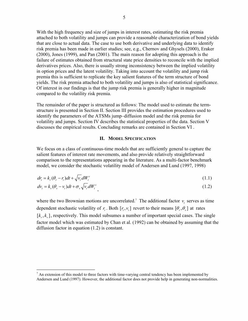
We focus on a class of continuous-time models that are sufficiently general to capture the salient features of interest rate movements, and also provide relatively straightforward comparison to the representations appearing in the literature. As a multi-factor benchmark model, we consider the stochastic volatility model of Andersen and Lund (1997, 1998)

( ) rt r r t t tdr k r dt v dWθ= − + (1.1)

( ) vt v v t v t tdv k v dt v dWθ σ= − + , (1.2)

where the two Brownian motions are uncorrelated.7 The additional factor tv serves as time dependent stochastic volatility of tr . Both [ , ]t tr v revert to their means [ , ]r vθ θ at rates [ , ]r vk k , respectively. This model subsumes a number of important special cases. The single factor model which was estimated by Chan et al. (1992) can be obtained by assuming that the diffusion factor in equation (1.2) is constant. 7 An extension of this model to three factors with time-varying central tendency has been implemented by Andersen and Lund (1997). However, the additional factor does not provide help in generating non-normalities.

6

Two factor Jump-Diffusion Models of Returns and Volatility Several recent papers examine interest rate models with jumps in interest rates (see Das (2001), Charko and Das (2000) and Johannes (2001)). While these papers incorporate jumps in returns, they exclude jumps in volatility, which lead to misspecification of the volatility term structure (see Eraker et. al. (2002)). Eraker et. al. find that jumps in returns can generate large movements, but the impact of a jump is transient in the sense that an impact of a jump in returns today has no impact on future distribution of returns. The specification below generalizes models of jumps in volatility and interest rates:

2

1 0( )( ) (1

r r rt r r t t t

t v v vt v v t t tv v

dr k r dW dNdt v

dv k v dW dNθ ξθ ξρσ ρ σ

⎛ ⎞− ⎛ ⎞ ⎛ ⎞⎛ ⎞ ⎛ ⎞= + +⎜ ⎟⎜ ⎟ ⎜ ⎟⎜ ⎟ ⎜ ⎟ ⎜ ⎟− −⎝ ⎠ ⎝ ⎠ ⎝ ⎠ ⎝ ⎠⎝ ⎠ .

(1.3)

where, r

tW and vtW are standard Brownian motions with correlation ( , )r v

t tcorr dW dW ρ= , rtN and v

tN are Poisson processes with intensities rλ and vλ , and rξ and vξ are the jump sizes in interest rates and volatility, respectively. This specification nests various popular models that have been used to price bonds. Restricting the jump intensities to zero

0r vλ λ= = and assuming that volatility is constant reduces the model to Vasicek (1977) specification. By assuming that jumps in interest rates are normally distributed

2~ ( , )rr rNξ μ σ and excluding jumps in volatility vλ , this nests jump-diffusion models by

Duffie and Kan (1995), Bas and Das (1997), Chacko and Das (2002) and Zhou (2001). Other models with jumps in volatility arriving independently from jumps in interest rates assume that ~ exp( )v

vξ μ , and jumps in returns follow 2~ ( , )rr rNξ μ σ . Singleton et. al specify a

model with contemporaneous arrivals, r vt t tN N N= = , and correlated jump sizes,

~ exp( )vvξ μ and 2| ~ ( , )r v v

r J rNξ ξ μ ρ ξ σ+ . Market Prices of Volatility and Jump Risk Process Given the presence of volatility and jump risks, this results in a non-unique pricing kernel due to the incompleteness of the market. Hence we use a candidate pricing kernel that is considered to be unique and makes the market complete. By assigning the market prices of risk, the dynamics of interest rates tr and volatility tv under the new martingale measure Q are now of the form

2

1 0( ) ( )( ) ( )(1

( )( )0( )

rt r r t t

t vt v v t v t tv v

r rJ J tt

v vt

dr k r dW Qdt v

dv k v v dW Q

t vdN Qdt

dN Q

θθ η ρσ ρ σ

η λξξ

⎛ ⎞− ⎛ ⎞⎛ ⎞ ⎛ ⎞= + ⎜ ⎟⎜ ⎟⎜ ⎟ ⎜ ⎟ ⎜ ⎟− + −⎝ ⎠ ⎝ ⎠ ⎝ ⎠⎝ ⎠

⎛ ⎞ ⎛ ⎞+ −⎜ ⎟ ⎜ ⎟

⎝ ⎠⎝ ⎠ ,

(1.4)

7

where [ ( ), ( )]r vt tW Q W Q is a standard Brownian motion under measureQ . The parameter vη

is the risk premia attached to varying volatility and ( )J J tt vη λ is the compensating term for the pure jump process ( )v

tN Q .

III. ECONOMETRIC APPROACH

First Stage Estimation When interest rates are described by a continuous time model with latent variables, a closed-form expression for the discrete-time transition density of the process is generally not available, and standard estimation techniques, such as maximum likelihood, cannot be easily used.8 Finding the conditional likelihood function of the state vector tX which has unanticipated jumps and unobservable factors is often infeasible. Several methods for the estimation of continuous-time models have been developed in recent years: among them include, Conley et. al. (1997), Hansen (1995), Jiang and Knight (1997), Johannes (1999), and Stanton (1997). Unfortunately, these methods are difficult to apply in the presence of both unobservable stochastic volatility and unanticipated jumps. Therefore, we resort to practical simulation methods for the evolution of the state vector proposed by Gallant and Tauchen (1996).9 This method involves summarizing the data by using a quasi maximum likelihood to project the observed data onto a transition density which is a close approximation to the true data generating process. This transition density is what Gallant and Tauchen refer to as an auxiliary model and its score is called the score generator for EMM. The primary advantage of this technique is that EMM estimates achieve the same degree of efficiency as the ML procedure if the auxiliary model asymptotically spans the score of the true model. It also provides powerful specification diagnostics that provide guidance in model selection. Detailed description of this estimation method is available in Gallant and Tauchen (1996) and Appendix I. Several applications can be found in Andersen, Benzoni and Lund (2001), Chernov and Ghysels (2000) and Chernov et. al. (1999, 2000). Second Stage Estimation for Identifying Risk Premia The second stage takes advantage of the estimated parameters for the state price density. Using the continuous time affine jump-diffusion models above, we adopt the derivations by Duffie, Pan and Singleton (2000) to derive the bond prices. The unique arbitrage-free price at time ( ), , ,t P t T X of a zero-coupon bond maturing at time ( )T t T≤ can be obtained as the

8 Even where maximum likelihood is in principle feasible, empirical applications are computationally challenging if the latent volatility variable has to be integrated out of the likelihood function.

9 Other simulation methods include the Monte Carlo Markov Chain method used by Elerain, Chib and Shephard (1998), Eraker (2001), Jacquier, Polson and Rossi (1994), Jones (1998) and Kim, Shephard and Chib (1998). Advances in Duffie, Pan and Singleton (2000) have inspired new methods based on empirical characteristic functions; see, e.g., Singleton (2001), Chacko and Viceira (1999), Jiang and Knight (1999) and Carrasco et al. (2000).

8

discounted expected value of the cash flow. In other words the prices of a bond that pays out one unit of account at maturity T is given by

( ) ( ), ,

Tu u ut

r X dQtP t T X E e

−⎡ ⎤∫= ⎢ ⎥⎣ ⎦ .

(1.5)

We compute the bond yields taking into account the estimated risk premia. The computed bond yields are a function of the estimated short-term interest rate tr , unobservable volatility factor tv , state price parameter vector θ and risk premium parameters ( ),v Jη η . The methodology followed is again the simulated method of moments approach where we minimize the bond yield errors. We assume that

~( , ) ( , , , , , , )t t v J tP T P T r vτ τ θ η η ε= + , (1.6)

where ( , )P Tτ is the observed bond yield and ~

(.)P is the predicted price using the ATSM. The error term is assumed to be stationary and egordic with zero mean. With this formulation we assume that the error term has zero mean and yields the moment condition

[ ]~

( , ) ( , , , , , , ) 0t t v JE P T E P T r vτ τ θ η η⎡ ⎤− =⎢ ⎥⎣ ⎦. (1.7)

The time τ bond yield are computed by solving numerically the ODE (1.4-1.5) which directly provide a closed form solution of bond yields.

IV. DATA SOURCES

Since there is no standard convention for reporting Brady bond yields, we resort to using the end of week bond yields as reported by Datastream from May 1994 through December 2002. The frequency of the data is weekly. The large standard deviations exhibited reflects the emerging market’s history of high increases in bond prices during crisis periods. It is also the case that Brady bond yields exhibit much higher kurtosis and skewness which suggests non-normality in the series. The non-normailities in the series are associated with different crises (Mexico, Asian and Russia) that might have spilled over to other emerging markets.

Mean S.D. Median Skewness Kurtosis

Argentina 33.7 80.2 14.8 5.4 33.3 Brazil 16.7 4.9 16.1 1.8 8.7

Brady Bond Price Statistics (1994-2002)

9

V. EMPIRICAL RESULTS

This section reports the EMM implementation of the various model specifications. First we discuss the SNP estimation results in section (A). Sections (B-D) discusses the EMM estimation results for the various models. Section E assesses the statistical significance of the market prices of risk and the economic relevance of risk premia in pricing bonds. Lastly, we compare the actual excess returns to the predicted excess returns for the various models.

A. SNP Model for Interest Rates

A successful application of EMM procedure requires choice of an auxiliary model that closely approximates the conditional distribution of the interest rate process. Once the score function of the auxiliary model asymptotically spans the score of the true model, then the EMM would be considered to be efficient. The SNP density estimation results are reported in Table 1. The SNP density is estimated for two data sets on interest rates of Argentina and Brazil. Rather than reporting the parameter estimates, we focus on the density structures as characterized by the trning parameter , , , , and u r g p z xL L L L K K . A description of these parameters is provided in the appendix. The different combinations of the tuning parameters provide different density functions as shown in panel B. Panel A reports the value of the Akaike information criterion (AIC), the Hannan and Quinn criterion (HQ) and the Schwarz Bayes information criterion (BIC). The Choice of the SNP model is based on the minimum (BIC) criterion. The main task of the nonparametric polynomial expansion in the conditional density is to capture any excess kurtosis in interest rates. For both series the semi parametric GARCH model is sufficient to capture the salient features of the data. The auxillary model for both series requires high order AR terms in the mean equation to capture the autocorrelation structure. A Garch(2,2) process is indicative of strong temporal persistence of the conditional variance. For all the series we note that there are non–Gaussian innovations as the BIC reduces with 0zK > . The case for heterogeneity in the polynomial expansion in xK is generally rejected as these terms are insignificant in all specifications. Since 0rL > in both cases, this implies that there are some ARCH effects in both series. For both the Argentina and Brazil interest rates series we need autoregressive terms in the mean uL to the order of 3.

10

B. Simple Model with Constant Volatility (CIR)

To obtain a bench mark, we estimate the CIR specification where volatility is considered to be constant and there are no surprising jumps. The model estimated is of the following form:

( )t r r t tdr k r dt r dWθ σ= − + . (1.8)

This model has been previously estimated in the literature by Chan et al (1992). Tables 2 and 3 (first columns) reports the parameter estimates, asymptotic t statistics and the EMM minimized criterion 2χ values. In all the series there appears to be strong evidence of mean reversion in the interest rate; the parameter rk is highly significant in both cases. While the parameter estimates of the diffusion model are significant, the 2χ tests for the goodness of fit strongly suggest that the model without varying volatility and jumps is highly mis-specified. For both series of Argentine and Brazil, the 2χ value are in excess of [58(13),29(10)]10 and can be rejected at the 95% confidence level. For Argentina, its also evident from these results that the EMM procedure can hardly accommodate any of the dominant SNP moments as most of the t -ratios in the SNP model are highly significant with this specification.11 The specification fails to accommodate the linear aspects of the data as indicated by large magnitude of the t -ratios on the mean scores of the parameters ( )1 3,ψ ψ . This simple CIR model also fails to account for the leptokurtic character of interest rate movements which is evident from the large t-ratios of the mean scores of the quadratic terms of the Hermite polynomial ( )02 03 05, ,a a a as shown in Table 5. While the ARCH like behavior of interest rates movements is well explained, the model fails to account for the persistence of volatility as indicated by the parameters ( )1 2,g gτ τ . For the Brazil series, the CIR model manages to fit the linear and AR behaviour of the data, but fails to accommodate the ARCH like behaviour of interest rates. Also of interest is the estimate for the constant variance σ which is approximately 7 percent for Argentina and Brazil, respectively. A comparison to the actual data shows that these EMM estimates are mainly explained by the poor fit of the constant variance model rather than a problem with the SNP model. Part of the reason why the diffusion coefficient tends to be estimated less precisely than the drift has been provided by Bandi and Phillips (2002). 12

10 Figures in parathensis are degrees of freedom.

11 Note that the standard errors computed using the EMM are biased upwards and the quasi t-ratios are downward biased relative to 2. Hence a t-statistic above 2 indicates failure of fitting a corresponding score.

12 They prove that consistent estimation of the drift requires a long time span and a high sampling frequency . Hence although daily data is short enough sampling frequency, the number of years used are not long enough time to estimate the drift.

11

C. Model with Stochastic Volatility (SV)

The basic one factor model is extended to a multifactor model with unobservable volatility. This estimation is performed with an assumption that Brownian motions are uncorrelated ( 0)ρ = . The extension improves the fit considerably as the Chi-Square statistics improves for both series. However for both series the stochastic volatility model is still strongly rejected. Part of the reason is that Brownian filtrations cannot reproduce the non-normalities inherent in interest rates. For the case of Argentina, this model generates more non-normalities like excess kurtosis as suggested by the insignificance of some of the Hermite polynomial coefficients (Tables 5 and 6). The exception is the even parameter 04a . It is well known that under the SNP, the even powers of the hermite function tend to control the tail thickness while odd powers control asymmetries. Hence this suggests that while this specification captures the asymetries in the data, it fails to accommodate the fat tails. The t -ratios of the mean function suggest that this specification fits the unconditional mean of the interest rate series. Unlike the previous case, this model fails to fit the scores of both the ARCH and GARCH parameters, which suggests that addition of stochastic volatility may not fully account for the persistence in volatility. Also, for the case of Brazil this model fails to fit SNP scores for both the ARCH and GARCH parameters. In summary, adding a stochastic volatility factor, while greatly improving the performance of the model, does not provide an adequate description of short-term interest rates for both series. The significance of the coefficients in the SNP model which describe excess Kurtosis clearly indicates that single and multi factor diffusion models do not generate enough non-normalities to match the amounts estimated from the short rate data. Dittmar and Gallant (2002) use various three factor affine and quadratic models and find that none of them can fit the tails of the distribution. Dai and Singleton (1999) find that three factor affine models cannot fit the non-normalities in swap rates as revealed by their specification tests. Hence adding more diffusion factors would not necessarily improve the fit as revealed by Audersen and Lund (1998) who use a three factor model with a stochastic central tendency.

D. Model with Varying Volatility and Jumps (SVJ)

With the failure of the popular diffusion models to generate non-normalities, we consider a simple stochastic volatility model which is augmented with a pure jump diffusion Poisson process with a Gaussian distribution of the jump size. The jump component is assumed to be constant with intensity: ( ) 0tλ λ= . The stochastic volatility model with jumps provides significant improvement over the earlier results. The Chi square test statistics for overall goodness of fit decrease to [20(8),15(5)]. So this model cannot be rejected at a 1% significance level. The parameters which characterize the mean, variance and frequency of jumps ( ), ,J J Jμ σ λ are all very significant. For the case of Argentina, it is found that on average there are 8.5 jumps per year. The variability and mean of jumps’ magnitude is also of interest. For instance in the case of Argentina the mean size of jumps over the period is

0.6± percent while their standard deviation is 0.4 percent. For the case of Brazil jumps occur

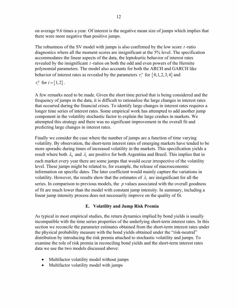
12

on average 9.6 times a year. Of interest is the negative mean size of jumps which implies that there were more negative than positive jumps. The robustness of the SV model with jumps is also confirmed by the low score t -ratio diagnostics where all the moment scores are insignificant at the 5% level. The specification accommodates the linear aspects of the data, the leptokurtic behavior of interest rates revealed by the insignificant t -ratios on both the odd and even powers of the Hermite polynomial parameters. The model also accounts for both the ARCH and GARCH like behavior of interest rates as revealed by the parameters { }for 0,1, 2,3, 4a

iτ and

{ } for 1, 2gi iτ = .

A few remarks need to be made. Given the short time period that is being considered and the frequency of jumps in the data, it is difficult to rationalize the large changes in interest rates that occurred during the financial crises. To identify large changes in interest rates requires a longer time series of interest rates. Some empirical work has attempted to add another jump component in the volatility stochastic factor to explain the large crashes in markets. We attempted this strategy and there was no significant improvement in the overall fit and predicting large changes in interest rates. Finally we consider the case where the number of jumps are a function of time varying volatility. By observation, the short-term interest rates of emerging markets have tended to be more sporadic during times of increased volatility in the markets. This specification yields a result where both 0λ and 1λ are positive for both Argentina and Brazil. This implies that in each market every year there are some jumps that would occur irrespective of the volatility level. These jumps might be related to, for example, the release of macroeconomic information on specific dates. The later coefficient would mainly capture the variations in volatility. However, the results show that the estimates of 1λ are insignificant for all the series. In comparison to previous models, the p values associated with the overall goodness of fit are much lower than the model with constant jump intensity. In summary, including a linear jump intensity process does not necessarily improve on the quality of fit.

E. Volatility and Jump Risk Premia

As typical in most empirical studies, the return dynamics implied by bond yields is usually incompatible with the time series properties of the underlying short-term interest rates. In this section we reconcile the parameter estimates obtained from the short-term interest rates under the physical probability measure with the bond yields obtained under the “risk-neutral” distribution by introducing the risk premia attached to stochastic volatility and jumps. To examine the role of risk premia in reconciling bond yields and the short-term interest rates data we use the two models discussed above:

• Multifactor volatility model without jumps • Multifactor volatility model with jumps

13

In the first model, since volatility is considered to be constant, the risk premia would come from the diffusive stochastic volatility. Introducing both stochastic volatility and jumps, we identify the additional risk premia associated with jumps. The estimation results are reported in Table 4. The volatility risk premium coefficient vη is estimated to be negative and significantly different from zero for the stochastic volatility model. This confirms the conjecture that variance risk is priced by the market. The size of the volatility risk premia is also of considerable magnitude. As discussed in the previous sections, stochastic volatility models tend to be highly mis-specified. Hence adding the jump component produces the non-normalities seen in the data. However, after establishing that jumps are common and of statistical significance, the next question then is how they are priced in the market. Considering the jump structure with time varying jumps we find that the jump risk premia for Argentine and Brazilian bonds are 0.256 and 0.339 basis points respectively. We only take into account the jump risk premia in sizes and assume that the risk premia attached to frequency of jumps is zero. Also of interest is the size of jump risk premia relative to volatility risk premia which is almost three times.

VI. CONCLUSION

The objective of this paper was to identify a class of diffusion models that are successful in approximating short-term interest rates for highly volatile markets. Estimation is undertaken by careful implementation of the EMM which provides powerful diagnostics for model choices. We find that models with only diffusive stochastic volatility in interest rates cannot fit the non-normalities in short-term interest rates for emerging markets. Adding jumps to the specification yields much more robust specifications which explain the leptokurtic behavior of interest rates especially in volatile markets. With a significant role played by jumps, this raises the question on how this risk is priced. There is strong evidence that investors attach a high risk premium to the frequent jumps in emerging market bond yields. For the case where jumps are more common, the jump risk premia are systematically higher that the volatility risk premia. Several extensions can be undertaken using this framework to address issues of contagious jumps from other markets. Also, if jumps are contagious, it may be possible to identify the risk premia attached to jumps from other countries.

14

APPENDIX I. SNP AUXILLIARY MODEL

Adopting Gallant and Tauchen’s method, we use the score function of an auxilliary model whose transition density is given by

( , )( , )

( , )f x y

f y xf x y dx

ρρ

ρ=∫

(A.1)

with parameter vector ρ . Expanding the function ( , )f x y ρ in a Hermite series and deriving the transition density of the truncated expansion then one obtains a transition density

1( )K t tf y x − that has the form of a location scale transform

1tt t xy Rz μ−

= + (A.2)

of an innovation tz .13 The density function of this innovation is

[ ][ ]

2

2

( , ) ( )( )

( , ) ( )K

p z x zh z x

p z x z du

φ

φ=∫ ,

(A.3)

where ( , )p z x is a polynomial in ( , )z x of degree K and ( )zφ denotes the multivariate normal density function with dimension M , mean vector zero and an identity variance-covariance matrix. The polynomial ( , )p z x can be expressed in rectangular form

0 0( , )

xz KK

p z x a x zβ αβα

α β= =

⎛ ⎞= ⎜ ⎟

⎝ ⎠∑ ∑

, (A.4)

where α and β are multi-indexes of maximal degrees zK and xK , respectively. The function ( , )p z x corrects for departures from Gaussianity. Various models can be derived from this specification. For the case of homogeneous innovations tz , the distribution does not depend on 1tx − and the density tz can be approximated by 2( ) [ ( )] ( )h z p z zφ→ where

( )p z is a polynomial of degree zK . The resulting density function is 2( ; ) [ ( )] ( , )M xf y x p z n yρ μ→ ∑ , where 1( )xz R y μ−= − . The leading term of the expansion

is ( , )M xn y μ ∑ , which is a Gaussian vector autoregression. When zK is positive, it’s a semi parametric VAR density which can approximate over a large class of densities can be derived. Other models can be derived by assuming that the leading term of the expansion

13 Further details of this derivation can be found in Gallant, Hsieh and Tauchen (1991).

15

1 1 1

't t tx x xR R− − −

∑ =

1 20 ( ) 11

( )r

t r t L ir

L

x i t L i xi

vech R P yρ μ− − − +− − +

=

= + −∑

1 1 1

't t tx x xR R− − −

∑ =

1 2 20 ( ) 1 ( )1 1

( ) ( ) ( )gr

t r t L i t L ir g

LL

x i t L i x i xi i

vech R P y diag G vech Rρ μ− − − + − − +− − +

= =

= + − +∑ ∑

( , )M xn y μ ∑ follows a Gaussian ARCH by letting R to be a linear function of the absolute values of elements of the vectors

1r t Lrt L xy μ− −− − through

21 tt xy μ−− − . The variance-covariance

matrix then becomes

(A.5),

where ( )vech R denotes a vector of length ( 1) / 2M M + containing elements of the upper triangle of R , 0ρ is a vector of length ( 1) / 2M M + , (1)P through ( )rLP are ( 1) / 2M M + by M matrices. Garch like specifications are can also be derived from:

(A.6),

where (1)G through ( )gLG are vectors of length ( 1) / 2M M + . In Summary, the tuning parameters of the SNP auxiliary model are

• zK degree of polynomial in z • xK degree of polynomial dependence on lags of tx • uL Lag Length of the VAR • rL Lag length of ARCH portion • gL Lag length of GARCH portion • pL Lag length of polynomial dependence on lags of tx

To find the appropriate tuning parameters we experiment with various versions of these models to select the best model using the Schwarz Bayes Information criterion (Schwarz, 1978) which is computed as:

^ 1( ) log( )2n

pBIC s n

nρρ= +

, (A.7)

where 11

1( ) log[ ( ; )]n

n t tt

s f y xn

ρ ρ−=

= − ∑ and the term (1/ 2)( / ) log( )p n nθ is the penalty to

good fits obtained by excessive parameterizations. The smaller the BIC the better the fit.

16

References

Andersen, T.G., L. Benzoni and J. Lund, 2001, An Empirical Investigation of Continuous-Time Equity Return Models, Journal of Finance, Vol. 57, pp. 1239-84.

Bansal, R., A.R. Gallant, R. Hussey and G. Tauchen, 1993, Computational Aspects of

Nonparametric Simulation, In D.A. Belsley (ed.) Computational Techniques for Econometrics and Economic Analysis, pp. 3-22.

Bansal, R., A.R. Gallant, R. Hussey and G. Tauchen, 1995, Non parametric Estimation of

Structural Models for High Frequency Currency Market Data, Journal of Econometrics, Vol. 66, pp. 251-287.

Benzoni, L., 2002, Pricing Options under Stochastic Volatility: An Empirical Investigation,

Working Paper, Finance Department-Calrson School of Management. Brennan, M.J. and E.S. Schwartz, 1980, Analyzing Convertible Bonds, Journal of Financial

and Quantitative Analysis, Vol. 15, pp. 907-929. Chacko, G. and L.M. Viceira, 1999, Spectral GMM Estimation of Continuous-Time

Processes, Working Paper, Harvard University. Chacko, G. and S. Das, 2002, Pricing Interest Rate Derivatives: A General Approach, Review

of Financial Studies, Vol. 15, pp. 195-241. Chan K.C., G.A. Karolyi, F.A. Longstaff, and A.B. Sanders, 1982, An Empirical Comparison

of Alternative Models of the Short Term Interest Rate, Journal of Finance, Vol. 47, pp. 1202-1227.

Chernov, M. and E. Ghysels, 2000, A Study Towards a Unified Approach to the Joint

Estimation of Objective and Risk Neutral Measures for the Purpose of Options Valuation, The Journal of Financial Economics, Vol. 56, pp. 407-458.

Conley, T.G., L.P. Hansen, E.G.J. Luttmer and J. Scheinkman 1997, Short term Interest

Rates as Subordinated Diffusions, The Review of Financial Studies, Vol. 10, pp. 525-577.

Cox, J.C., J.E. Ingersoll, and S.A. Ross, 1985, A Theory of the Term Structure of Interest

Rates, Econometrica Vol. 53, pp. 385-407. Das, S., 2001, The Surprise Element: Jumps in Interest Rates, Journal of Econometrics, Vol.

106, pp. 27-65. Duffie, G.R., 2002, Term Premia and Interest Rate Forecasts in Affine Models, Journal of

Finance, Vol. 57, pp. 405-443.

17

Duffie, D. and K.J. Singleton, 1993, Simulated Moments Estimation of Markov Models of Asset Prices, Econometrica, Vol. 61, pp. 929-952.

Duffie, D., J. Pan and K.J. Singleton, 2000, Transform Analysis and Option Pricing for

Affine Jump Diffusions, Econometrica, Vol. 68, pp. 1343-1376. Duffie G.R. and R. Kan, 1996, A Yield Factor Model of Interest Rates, Mathematical

Finance, Vol. 6, pp. 379-406. Eraker, B., 2000, Do Stock Prices and Volatility Jump? Reconciling Evidence from Spot and

Option Prices, Working Paper, University of Chicago. Gallant, A.R. and G. Tauchen, 1989, Semi nonparametric Estimation of Conditionally

Constrained Heterogeneous Processes: Asset Pricing Applications, Econometrica, Vol. 57, pp. 1091-1120.

Hansen, L.P. 1982, Large Sample Properties of Generalized Method of Moment Estimators,

Econometrica, Vol. 50, pp. 1029-1056. Jacquier, E.N., g. Polson and P.E. Rossi, 1994, Bayesian Analysis of Stochastic Volatility

Models, Journal of Business and Economic Statistics, Vol. 12, pp. 371-389. Jiang, G. and J.L. Knight, 1999, Efficient Estimation of the Continuous Time Stochastic

Volatility Model via the Empirical Characteristic Function, Journal of Business and Economic Statistics.

Johannes, M., 2001, The Statistical and Economic Role of Jumps in Continuous-Time

Interest Rate Models, Working Paper, Columbia University. Johannes, M., 1999, A Nonparametric Approach to Jumps in Interest Rates, Working Paper,

Columbia University. Jones, C.S., 1999, The Dynamics of Stochastic Volatility: Evidence from Underlying and

Option Markets, Working Paper, Rochester University. Merton, R.C., 1973, Theory of Rational Option Pricing, Bell Journal of Economics and

Management Science, Vol. 4, pp. 141-183. Pan, J., 2002, The Jump-Risk Premia Implicit in Options: Evidence from an Integrated Time

Series Study, Journal of Financial Economics, Vol. 63, pp. 3-50. Schaefer, S. and E.S. Schwartz, 1984, A Two Factor Model of the Term Structure: An

Approximate Analytical Solution, Journal of Financial and Quantitative Analysis, Vol. 19, pp. 413-424.

18

Singleton, K.J., 2001, Estimation of Affine Asset Pricing Models Using the Empirical Characteristic Function, Journal of Econometrics, Vol. 102, pp. 111-141.

Vasicek, O., 1977, An Equilibrium Characterization of the Term Structure, Journal of

Financial Economics, Vol. 5, pp. 177-188.

19

Panel B: ==================================================== Parameter Setting Density Function

uL gL rL pL zK xK 0 0 0 ≥ 0 0 0 iid Gaussian >0 0 0 ≥ 0 0 0 Gaussian VAR >0 0 0 ≥ 0 >0 0 Semiparametric VAR ≥ 0 0 >0 ≥ 0 0 0 Gaussian ARCH ≥ 0 0 >0 ≥ 0 >0 0 Semiparametric ARCH ≥ 0 >0 >0 ≥ 0 0 0 Gaussian GARCH ≥ 0 >0 >0 ≥ 0 >0 0 Semi parametric GARCH ≥ 0 ≥ 0 ≥ 0 >0 >0 >0 Nonlinear Nonparametric

====================================================

Panel A Data type Lu Lg Lr Lp Kz Iz Kx Ix Sn AIC HQ BIC

Argentina 0 0 0 2 0 0 0 0 1.4253 1.4263 1.4273 1.42913 0 0 1 0 0 0 0 -0.2458 -0.2432 -0.2406 -0.23623 0 0 1 1 0 0 0 -0.3239 -0.3209 -0.3178 -0.31243 0 4 1 0 0 0 0 -0.4476 -0.4430 -0.4383 -0.43033 0 4 1 2 0 0 0 -0.5160 -0.5104 -0.5047 -0.49493 2 4 1 0 0 0 0 -0.4922 -0.4867 -0.4809 -0.47113 2 4 1 2 0 0 0 -0.5467 -0.5401 -0.5333 -0.52173 2 4 1 2 0 1 0 -0.5561 -0.5480 -0.5397 -0.5254

Brazil 0 0 0 1 0 0 0 0 1.3882 1.3892 1.3903 1.39213 0 0 1 0 0 0 0 -0.6842 -0.6816 -0.6790 -0.67463 0 0 1 1 0 0 0 -0.7674 -0.7643 -0.7612 -0.75593 0 4 1 0 0 3 2 4 1 0 0 0 0 -1.0430 -1.0374 -1.0317 -1.02193 2 4 1 1 0 0 0 -1.0751 -1.0685 -1.0617 -1.00513 2 4 1 1 0 1 0 -1.0669 -1.0588 -1.0504 -1.0361

1/ The SNP density is estimated for short-term interest rates. Panel above reports the structuree of the estimated densities and values of the objective function sn, values of the Akaike Infoprmation Criterion (AIC), the Hannan and Quinn criterion (HQ) and the Schwarz Bayes Information criterion (BIC)

.

Table 1: SNP Density Estimation 1/

20

Table 2. EMM Estimates of the Jump Diffusion Stochastic Model for Argentina

Estimates are for the sample period October 1994 to December 1999. Standard errors are reported in brackets. ==========================================================

Parameter CIR SV SVJ1 SVJ2

rk 0.9814 1.3243 0.8988 1.4555 (0.0910) (0.2430) (0.0112) (0.1350)

rθ 6.2780 6.2191 6.1406 6.4192 (0.5257) (0.4352) (0.5263) (0.3213)

vk 0.1139 0.5235 0.5051 (0.0403) (0.0551) (0.0135)

vθ 0.6466 0.4805 0.3870 (0.6341) (0.2337) (0.2134)

rσ 0.0735 (0.0103)

vσ 0.0855 0.0679 0.0967 (0.0220) (0.0321) (0.0631)

Jμ 0.3274 -0.6026 (0.0398) (0.1043)

Jσ 0.2606 0.4090 (0.0356) (0.1322)

0λ 8.6321 8.5120 (3.4522) (2.3211)

1λ 2.4955 (1.9321)

2[ . .]d fχ 58.50[13] 21.58[10] 20.34[8] 20.88[7]

21

Table 3. EMM Estimates of the Jump Diffusion Stochastic Model for Brazil

Estimates are for the sample period October 1994 to December 1999. Standard errors are reported in brackets. ==========================================================

Parameter CIR SV SVJ1 SVJ2

rk 0.8637 1.0107 0.7240 0.7293 (0.0984) (0.1056) (0.0602) (0.1192)

rθ 6.1370 5.7419 8.7012 7.7512 (0.6541) (0.4981) (0.3822) (0.4954)

vk 1.3328 1.2797 1.1958 (0.1089) (0.0606) (0.0628)

vθ 0.8305 0.8321 0.3471 (0.2412) (0.2476) (0.0293)

rσ 0.2228 (0.1239)

vσ 0.3443 0.7212 0.0636 (2.0342) (1.2156) (0.0519)

Jμ -1.6966 0.2386 (0.1004) (0.5934)

Jσ 1.7405 1.3245 (0.1145) (0.2219)

0λ 9.5603 9.6321 (2.4503) (2.1146)

1λ 0.2240 (1.4521)

2[ . .]d fχ 29.30[10] 28.65[7] 15.20[5] 22.13[4]

22

Table 4. Volatility and Jump Risk Premia ====================================================== Brazil Argentina Parameter SV SVJ SV SVJ

vη -0.4325 -0.1123 -0.3934 -0.0821

(0.0476) (0.0511) (0.0389) (0.0465) Jη 0.3397 0.2561

(0.9766) (0.1176)

23

Tab

le 5

. Est

imat

es a

nd t-

ratio

s of t

he A

vera

ge S

NP

Scor

e C

ompo

nent

s for

Arg

entin

a =

====

====

====

====

====

====

====

====

====

====

====

====

====

====

====

====

====

====

====

====

====

====

====

====

====

====

====

====

====

===

Para

met

er

CIR

SV

SV

J

SVJ1

H

erm

ite

01a

0

.881

(0.8

9)

0.

725

(0

.73)

-0.1

19

(-

0.12

)

0.09

3

(0.0

9)

02a

-6

.530

(-1.

99)

1.

401

(0

.43)

-0.9

80

(-

0.30

)

-5.2

27

(-

1.59

)

03a

3.

742

(1

.55)

2.35

4

(0.9

7)

1.

809

(0

.75)

4.31

8

(1.7

8)

04a

-2

1.97

1

(-3.

19)

-1

3.49

8

(-1.

96)

-2

.523

(-0.

37)

-3

.977

(-0.

57)

05a

6.

435

(1.3

4)

4.

651

(0

.97)

0.49

4

(0.1

0)

2.

634

(0

.55)

A

R

1

ψ

-40.

114

(-

2.29

)

-9.0

12

(-

0.52

)

-19.

614

(-

1.12

)

-32.

552

(-

1.86

)

2ψ

21.7

20

(1

.75)

14.8

59

(1

.20)

17.9

74

(1

.45)

21.0

87

(1

.70)

3ψ

24.3

64

(1

.99)

16.5

44

(1

.35)

18.7

13

(1

.53)

23.9

55

(1

.95)

4ψ

18.2

48

(1

.48)

12.9

73

(1

.05)

15.1

91

(1

.23)

21.3

59

(1

.73)

A

RC

H

0a τ

-126

.258

(-

2.28

)

-90.

099

(-

1.63

)

-67.

305

(-

1.21

)

-73.

704

(-

1.33

)

1a τ

-4

.831

(-1.

35)

-5

.680

(-1.

58)

-0

.321

(-0.

09)

-0

.870

(-0.

24)

2a τ

-6

.323

(-1.

71)

-6

.089

(-1.

65)

-1

.635

(-0.

44)

-2

.299

(-0.

62)

3a τ

-3

.476

(-1.

03)

-5

.236

(-1.

55)

-0

.723

(-0.

21)

-0

.977

(-0.

30)

4a τ

-3

.437

(-1.

05)

-4

.041

(-1.

23)

-2

.421

(-0.

74)

-0

.074

(-0.

02)

GA

RC

H

1g τ

-1

8.36

7

(-2.

38)

-1

4.99

0

(-1.

95)

-8

.013

(-1.

04)

-8

.195

(-1.

06)

2g τ

-1

7.13

1

(-2.

27)

-1

4.34

2

(-1.

90)

-7

.402

(-0.

98)

-7

.731

(-1.

02)

24

Tab

le 6

. Est

imat

es a

nd t-

ratio

s of t

he A

vera

ge S

NP

Scor

e C

ompo

nent

s for

Bra

zil

===

====

====

====

====

====

====

====

====

====

====

====

====

====

====

====

====

====

====

====

====

====

====

====

====

====

====

====

====

====

=

Para

met

er

CIR

SV

SV

J

SVJ2

H

erm

ite

01a

0.

506

(0

.12)

0.67

8

(0.1

7)

1.

035

(0

.25)

-0.3

19

(-

0.07

8)

02a

1.

918

(0

.23)

2.09

3

(0.2

5)

5.

330

(0

.64)

-2.6

04

(-

0.31

3)

AR

0ψ

23.1

50

(0

.58)

20.8

22

(0

.52)

24.3

15

(0

.60)

14.7

56

(0

.367

)

1ψ

-24.

785

(-

0.91

)

-23.

490

(-

0.86

)

-20.

673

(-

0.76

)

-9.2

54

(-

0.34

0)

2ψ

-21.

593

(-

0.81

)

-20.

546

(-

0.77

)

-17.

855

(-

0.67

)

-5.9

67

(-

0.22

3)

3ψ

-22.

720

(-

0.82

)

-20.

045

(-

0.72

)

-19.

793

(-

0.71

)

-7.5

83

(-

0.27

4)

AR

CH

0a τ

60

.255

(0.4

6)

52

.628

(0.4

0)

20

.146

(0.1

5)

-8

1.81

7

(-0.

621)

1a τ

11

.606

(2.1

9)

10

.693

(2.0

2)

9.

668

(1

.82)

5.79

6

(1.0

93)

2a τ

10

.786

(1.8

1)

10

.155

(1.7

1)

8.

556

(1

.44)

5.96

3

(1.0

02)

3a τ

9.

430

(1

.57)

9.94

0

(1.6

5)

8.

185

(1

.36)

4.99

8

(0.8

31)

4a τ

9.

754

(1

.74)

10.2

65

(1

.84)

7.51

7

(1.3

4)

6.

158

(1

.101

) G

AR

CH

1g τ

14.3

24

(1

.07)

13.2

36

(0

.99)

11.7

51

(0

.88)

-0.0

93

(-

0.00

7)

2g τ

15

.805

(1.2

1)

14

.945

(1.1

4)

12

.948

(0.9

9)

1.

617

(0

.124

)

25

Figure 1. SNP Sample Forecasts and Actual Data for Argentina and Brazil