Vol. 14, No. 4, June 2006, 351–363

Administrator

Oval

Inverse Problems in Science and EngineeringVol. 14, No. 4, June 2006, 351–363

Inverse problem of aircraft structural parameter

estimation: application of neural networks

P. M. TRIVAILO*y, G. S. DULIKRAVICHz,D. SGARIOTOx and T. GILBERT�

ySchool of Aerospace, Mechanical and Manufacturing Engineering,RMIT University, Melbourne, Victoria, Australia

zDepartment of Mechanical and Materials Engineering,Florida International University, Miami, Florida, USA

xSchool of Aerospace, Mechanical and Manufacturing Engineering,RMIT University, Melbourne, Victoria, Australia

�School of Aerospace, Mechanical and Manufacturing Engineering,RMIT University, Melbourne, Victoria, Australia

(Received 10 January 2005; revised 8 April 2005; in final form 20 May 2005)

In this article, a novel method for estimating inertial and stiffness parameters for aircraftstructures is presented. The method is based on a combination of the finite element method(FEM) and artificial neural networks (ANNs). ANNs are known for their non-linearityand input/output mapping features and the proposed procedure aims to develop networkarchitecture and training data capable of overcoming many of the shortfalls associated withprevious parameter estimation techniques, such as uniqueness of solution and inadequateperformance in the presence of uncertainties. The proposed parameter estimation techniqueis used to determine inertial and stiffness properties of a linear FEM comprised of planarHermitian beam elements. It achieves this with surprising accuracy. The stiffness distribu-tion is estimated from static load/deformation considerations, while the inertial distributionis estimated from the modal characteristics of the model. Finite Element Analysisin MATLAB� is used to generate the training data for the networks, which are simulatedusing its Neural Network Toolbox.

Keywords: Neural networks; Parameter estimation; Aircraft structures; Finite elements

2000 Mathematics Subject Classifications: 70F17; 82C32; 74S05; 93A30; 62M451

*Corresponding author. Email: [email protected]

Inverse Problems in Science and Engineering

ISSN 1741-5977 print: ISSN 1741-5985 online � 2006 Taylor & Francis

http://www.tandf.co.uk/journals

DOI: 10.1080/17415970600573411

1. Introduction

1.1. Preface

As the demand for aerospace structures with greater reliability and efficiency increases,so do the levels of complexity and computationally demanding analysis requiredto engineer them. Classical techniques consistently fail to have adequate robustness anddexterity when adapted to modern engineering problems. There is compelling evidencethat Soft Computing techniques like Artificial neural networks (ANNs) hold the key tosolving traditionally awkward engineering problems by basing them on novelapproaches existing in nature. Mathematically speaking, the inverse problem isill conditioned, hence solution uniqueness is not guaranteed. It is here that traditionaltechniques begin to falter, and those such as ANNs flourish. Since the taskof identifying aircraft structural parameters is an Inverse Problem, the proposedapplication of ANNs to parameter identification is anticipated to be a powerful anduseful means of addressing the many issues that arise when such a taxing taskis undertaken.

1.2. Literature review

Currently, there is little research activity involving the application of ANNs toparameter identification techniques for aircraft wing structures, making the researchdetailed here truly novel. There exists a large research effort into the applicationof single objective [1] and multi-objective [2] optimization techniques to the task ofwing parameter identification, which for the most part are ‘direct’ approaches to theproblem; however their usefulness has not been discounted.

The centre of most of the research regarding parameter identification for aircraftstructures is in the area of genetic algorithms [2]. Although being based on frequencyresponse functions (FRFs), which are not pursued in the method proposed here,this work did prove very useful in shedding light as to the major limitations andshortfalls associated with both conventional and unconventional parameter estimationtechniques. These were namely the existence and uniqueness of a solution andthe ‘curse of dimensionality’.

A technique being researched increasingly in the field of parameter estimation isthat of model updating, which seeks to marry the fields of ANN and the finite elementmethod (FEM) [3]. While quite juvenile in its development, it promises to be anexceptionally powerful technique for aircraft wing modelling and parameter estimation.While not directly used in this research task due to its high complexity and advancednature, it provides a direction for further research activities.

There also exists a large body of research regarding static and dynamic modellingof ‘equivalent aircraft wing structures’. By either employing equivalent beam-rodaircraft wing models [4], equivalent plate models [5], or equivalent skin models [6], thesetechniques aim solely to replace complex physical aircraft wings with simplified andequivalent models that accurately mimic the performance of the actual physical wings.Most of these studies are rather specific and problem dependent in their development,and have the main limitation of being ‘direct/conventional’ approaches to the problemof aircraft wing structural parameter identification, which is an approach avoided here.It is anticipated that while this body of knowledge is not entirely aligned with the

352 P. M. Trivailo et al.

proposed research, it still provides useful insight into conventional parameterestimation techniques.

1.3. Background into neural networks

An ANN is an enormously distributed parallel processing unit, consisting of simplerindividual processing units which have inherent tendencies to store and retrieveobserved knowledge [7]. ANNs resemble the human brain, in that they acquireknowledge and information from their environment which is stored within inter-neuronconnections.

ANNs derive their problem-solving prowess from their massively parallel architec-ture and ability to learn and generalize. They also possess input/output mappingcapabilities, adaptivity, robustness and an ability to cope with non-linearity. Thesetraits assist ANNs in solving complex and large-scale (e.g. inverse) problems thatare currently unsympathetic to solution.

The Neural Networks utilized here are implemented using the MATLAB� NeuralNetwork Toolbox. The reader is referred to [7] and [8] for further informationon Neural Networks and their implementation.

2. Parameter estimation using neural networks

2.1. Model development

In order to apply ANNs to the estimation of aircraft structural parameters, it isnecessary to construct a simplified, but representative model of the desired structuralcomponent. As this study deals solely with the estimation of inertial (�A) and stiffness(EI ) parameters of a cantilevered beam, representative of a real aircraft wing,an appropriate finite element cantilevered beam model was chosen. A schematic of thebeam model can be seen in figure 1.

Once a suitable model of the wing has been constructed and the properties of themodel that are to be identified established, exactly how these properties are to beestimated needs to be ascertained. Hence, it is also necessary to obtain some empiricalor numerical data regarding the mechanical behaviour of the cantilevered beam, whichwill be used as a gateway for establishing the desired inertial and stiffness parameters.

EIi, rAi

Li

Figure 1. Cantilevered beam model of a real aircraft wing.

Inverse problem of aircraft structural parameter estimation 353

This is the essence of ANN training. In this article, two sets of simulated numerical

data form the basis of the training data for the ANNs. The first are deformation

characteristics of the beam model when subjected to a variety of static loads, whilst

the second is the modal characteristics of the beam model from an eigenvalue analysis.

In practice, these data sets may be sought from actual experiments undertaken directly

on the structure under consideration. Alternatively, the data sets may be synthesized

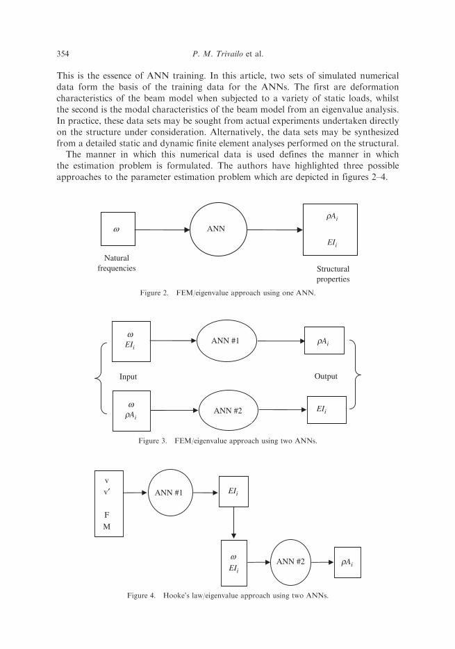
from a detailed static and dynamic finite element analyses performed on the structural.The manner in which this numerical data is used defines the manner in which

the estimation problem is formulated. The authors have highlighted three possible

approaches to the parameter estimation problem which are depicted in figures 2–4.

ω ANN

Naturalfrequencies

EIi

Structuralproperties

rAi

Figure 2. FEM/eigenvalue approach using one ANN.

OutputInput

wrAi

ANN #2

ANN #1

EIi

wEIi

rAi

Figure 3. FEM/eigenvalue approach using two ANNs.

rAiωEIi

vv′

F

M

ANN #1

ANN #2

EIi

Figure 4. Hooke’s law/eigenvalue approach using two ANNs.


Approach 1 involved establishing a single ANN which takes natural frequencies (!)as inputs, and determines �A and EI for each beam element in the model. Training data

was developed by solving the eigenvalue problem for models with varying mass and

stiffness properties. A diagram of this approach is shown in figure 2.Approach 2 utilized two ANNs; the first takes natural frequencies (!) and EI

as inputs, and outputs �A, while the second takes natural frequencies and �A as inputs

to determine EI. The training data was developed in the same manner as for the first

approach. A diagram of this approach is shown in figure 3.In Approach 3, �A and EI for each element in the beam model is estimated using

two different ANNs using two entirely different approaches. The stiffness properties

are estimated from static load/deformation considerations, while the inertial properties

are estimated from an eigenvalue formulation of the model. Hence, two sets of training

data are simulated, the first by using Hooke’s law to find EI from load/deformation

data, and the next by conducting the direct eigenvalue problem for the beam model,

calculating the natural frequencies of the beam from �A and EI. Upon training, one

ANN shows load/deformation data to yield elemental stiffnesses, while the other ANN

shows the previously calculated EI values, as well as the natural frequencies of the beam

model, to yield �A.Hence, the problem reduces to first estimating EI for each beam element from

load/deformation data of the beam model, and then estimating �A from both the

natural frequencies of the beam and the previously estimated EI values. This approach

is depicted in figure 4.After considerable investigation into which of the three approaches was most

feasible for the task considered here, it was found that Approach 3 was the most

flexible, more manageable and had fewer inherent deficiencies and limitations.

Approach 1 was found to be the most impractical and most difficult to implement.

This is mainly due to the fact that, no matter how many elements were used to model

the beam, the resulting network was forced to estimate more parameters than it was

provided with (the size of the output vector was always greater than the size of the

input vector). Such a situation is not at all favourable for ANNs.Approach 2 attempts to overcome the adverse problems associated with Approach 1

by reducing the size of the output vector and correspondingly increasing the size of the

input vector, through the use of two ANNs. However, this approach encounters grand

problems of its own, which are tied to the nature of eigenvalue problems. The natural

frequencies of a mechanical system are dependent on the mass and stiffness

distributions of that system, hence the frequencies can be thought of as a function

of mass and stiffness. In Approach 2, it is assumed that either the mass or stiffness

distribution of the beam is initially known. In general, this will not be the case, and

it imposes severe limitations on the applicability and generality of the parameter

estimation procedure. Thus it was not considered here.Hence, Approach 3 is the nominated procedure for estimating the inertial and

stiffness properties of the beam model. Of all the three approaches, it is the most

physically intuitive method, relying heavily on real physical relationships between

parameters. This is a very important consideration, since most techniques used to

solve inverse problems are very much ‘black box’ approaches, with little regard for

the underlying physical relationships relating system parameters. While not entirely

‘white box’ modelling, Approach 3 is an example of ‘grey box’ modelling.


2.2. Training process

Once a suitable model of the beam has been developed, and an approach to solvingthe task has been decided on, the aspect of simulating training data needs to beaddressed. Consisting of input and output pairs, this data is fed into the ANN,which uses it to model the underlying relationship between the input and the output.In this article, two sets of training data are needed, one for the ANN used to estimatestiffness properties, and another set for the ANN used to estimate the inertialproperties. Means of constructing each of these training data sets will be discussedseparately next.

2.3. Generation of training data

The generation of the training data sets for the ANNs is quite similar, and only theset used to estimate the bending stiffness of the beam model will be presented. This dataset is produced by solving the Hooke’s law problem for many beam models that couldbe used to represent the real structure. (The other is produced by solving manyeigenvalue problems.) This process was employed since the opportunity to undertakenumerous repeated experiments on a physical real aircraft wing is not available to theauthors. The procedure for generating the required numerical training data for one suchbeam model of an aircraft wing is detailed next.

(a) Firstly, the bending stiffness EI for each element used to represent the beamis generated using a random number generator. This generator produces a numberfor each EI value in the interval [0, 1], which is then weighted, so that the valuesare representative of a realistic tapered cantilever beam (i.e. mass and stiffnessproperties are reduced in span-wise direction from the supported end of the beamto the free end).

(b) Similarly, the magnitude of the slope at each node, for each beam element,is generated randomly and appropriately weighted. Since the beam is to becantilevered, the condition of zero slope at one end of the beam is enforced.

(c) By integrating the slope vector, the deflection at each node can be found.Similarly the condition of zero deflection at one end of the beam is enforced.

(d) Next, the deflection and slope data are assembled into a global deflection vectorwhich will be used during the finite element Hooke’s law formulation.

(e) The elemental stiffness matrices for the beam model are calculated using thestiffness and geometric data for each element of the beam model. These elementalstiffness matrices are appropriately assembled into a global stiffness matrix,which, upon the application of appropriate boundary conditions, will be usedduring the finite element Hooke’s law formulation.

(f) The Hooke’s law problem is solved, using the global stiffness and displacementvectors, to calculate the forces and moments at each node in the beam. Hence,the nodal forces and moments for each element in the beam are calculatedfrom the global stiffness and deflection matrices.

(g) The force/moment and deflection/slope data is assembled into a vector, which willserve as the input vector for the ANN during training. The output (known duringtraining as the target vector) will be the EI values for each element of the beammodel. The numbers within each of these vectors are appropriately scaled so thatall numbers lie within the interval [0, 1], needed for enhanced ANN training.


(h) The resulting input/output training data pairs are saved for future networktraining.

2.4. Simulation of testing data

In order to assess the performance of the two ANNs at estimating the requiredstructural properties for the beam model, testing data is needed for the two ANNs.This testing data takes exactly the same form as the training data, and is simulatedin exactly the same fashion as the two training data sets, except for one subtledifference. The testing data, although resembling the training data, should take onslightly different values, so as to test if the network can generalize sufficiently, and notjust memorize the training data. Hence, the size of the testing data sets are much smallerthan the training data sets, but must fall within the global range that the training dataencompasses, otherwise the generalizing process will be compromised. In other words,for each ANN, a large data set is created using the process outlined in section 2.3.From each of these sets, a smaller subset is removed and set aside to be used to testthe generalization capability of each ANN.

2.5. Network construction and simulation

Upon construction of the two sets of training data, the two ANN are constructed andsimulated; one ANN used to estimate stiffness properties, and the other ANN used toestimate the inertial properties. Means of constructing each of these ANN are discussedbelow. Since the construction, training, testing and simulation of each of the two ANNare very similar, each is discussed concurrently.

2.6. ANN used to estimate stiffness and inertial properties

These networks are constructed, trained, tested and simulated, producing the requiredstructural properties of the beam model, using the procedure detailed next.

(a) Firstly, the relevant training and testing data sets are loaded into the workingenvironment. A global data set of size 2500 is generated for each ANN, whichis partitioned into two smaller subsets, one for training and one for testing.Each training data set contains 2475 unique input/output pairs, while each testing setcontains 25 unique input/output pairs, sampled at equally spaced intervals from theglobal data set, which are not seen by their relevant ANN.

Since there are no rigid and well-defined procedures to adhere to when determiningthe size of the training data required for both learning and adequate generalization [7],the optimal size of the training data for each ANN was determined empirically.This is meant that a large portion of research involved addressing these issues. It wasfound that a training data size of 2500 was the minimum possible for efficient networktraining and adequate generalization (for the most optimum network architecturediscussed subsequently).(b) Next the ANN is constructed, by specifying the following:

The architecture of each ANN, hence the number of layers and number of neuronsin each layer. Both ANN contain two hidden layers, and along with an input and


output layer and have a total of four layers. Both ANN contain 15 neurons in the firsthidden layer, 10 in the second and four neurons in the output layer.

Two hidden layers were chosen since they represent the lower limit for the solutionof inverse problems using ANNs. Since the number of neurons in the output layer mustbe equal to the size of the output vector, four neurons were used in the output layer.The number of neurons in the first and second hidden layers was empiricallydetermined, again due to the scarcity of routine techniques used for optimal neurondetermination. After much consideration between learning efficiency, network perfor-mance and training time, for both ANN, the optimum number of neurons in the firstand second hidden layers was found to be 15 and 10 respectively.

The type of activation function used by each neuron, in each layer for each ANN.The neurons in each of the hidden layers for both ANN use the sigmoid type activationfunction to accommodate non-linearity, while the output neurons use linear activationfunctions so that the ANN outputs can take on any real number.

The training algorithm to be used for each ANN, along with its performancefunction, the number of times the training data set is to be shown to the ANN(epochs), along with the stopping criteria. The ANN used to estimate the bendingstiffness properties of the beam uses the Levenberg–Marquardt training algorithm,which is an enhanced quasi-Newton numerical optimization training method. TheANN used to estimate the mass properties of the beam uses the Resilient BackPropagation training algorithm, which is an enhanced Steepest Descent trainingmethod with modest memory requirements. Both ANN use the sum square error(SSE) performance function to assess network performance, with the stoppingcriteria being the zero error condition. The total number of epochs for the ANNused to estimate the bending stiffness properties of the beam is 100, while the totalnumber of epochs for the ANN used to estimate the mass properties of thebeam is 5000. These epoch numbers ensure adequate network convergence forboth ANNs.

The Levenberg-Marquardt training algorithm was chosen for the ANN used toestimate the bending stiffness of the beam since it is accepted to be the fastest methodfor training moderate-sized feed forward ANNs and has very efficient implementationin the MATLAB� environment [8]. However, it does suffer from the burden of beingvery ‘memory-intensive’ if the size of the network is sufficiently large, like the casefor the mass estimation ANN. Due to its much larger input vector, the ANN usedto estimate the mass distribution of the beam required a different training algorithm.The Resilient Back Propagation training algorithm was found to be the quickest andleast ‘memory-intensive’ of the training algorithms available in the Neural NetworkToolbox, hence its use in training the ANN used to estimate the mass distributionof the beam. While the Resilient Back Propagation training algorithm is less‘memory-intensive’ and as fast as the Levenberg-Marquardt training algorithm,it requires more epochs (presentation of training data samples) to learn the underlyingrelationships within the training data.(c) The ANNs are then trained accordingly, with post-training regression analysiscarried out to assess the performance of training. The results of network training for theANN used to estimate the bending stiffness are shown in figure 5.

With reference to figure 5, it is evident that the network error goal for the ANNwas not met. However after 100 epochs, it can be seen that the network error associatedwith the ANN has converged to a final value, indicating that further training will not


improve network performance. A similar phenomenon occurred for the additionalANN employed for inertial property estimation.(d) The ANN is then presented with the testing data sets, and is required to producean estimate of the stiffness and inertial properties for the beam models. Post-testingregression analysis is carried out to assess the ANN’s ability to generalize. The resultsof post-testing regression analyses for the ANN used for bending stiffness estimationis shown in figure 6.

Figure 6 illustrates the ability of the ANN to estimate the stiffness properties of eachelement for each beam model used to test the network. This ANN can very accuratelyestimate the stiffness properties of each element for beam models it has not seenbefore. This is reinforced upon observation of the correlation coefficients (R-values)for each element in both the figure, which are all very close to unity, indicating goodgeneralization and accuracy when estimating structural properties of cantileveredbeams. Similar results were found for the ANN used to estimate the inertial propertiesof the beam model.

0 20 40 60 80 100

104

102

100

10−2

100 EPOCHS

TR

AIN

ING

-SO

LID

TE

ST-D

ASH

ED

PERFORMANCE IS 0.512903, GOAL IS 0

Figure 5. Evolution of network training/testing error for bending stiffness estimation.

0.46 0.51 0.570.46

0.51

0.57

0.36

0.41

0.47

0.24

0.29

0.34

0.11

0.17

0.23

ELEMENT 1

0.36 0.41 0.47 0.24 0.29 0.34

ELEMENT 2 ELEMENT 3

0.11 0.17 0.23

ELEMENT 4

NE

TW

OR

K E

STIM

AT

E NETWORK TARGET

R = 0.99 R = 0.975 R = 0.972 R = 0.95

Figure 6. Network post-testing regression analysis for bending stiffness estimation.


(e) The ANN estimates of the stiffness and inertial properties are compared against thetarget vectors within the relevant testing data sets, and the relative error is calculated.(f ) The ANN and all their associated characteristics are stored for future analysis.

3. Evaluative example

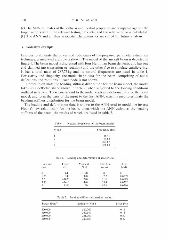
In order to illustrate the power and robustness of the proposed parameter estimationtechnique, a simulated example is shown. The model of the aircraft beam is depicted infigure 1. The beam model is discretised with four Hermitian beam elements, and has oneend clamped (no translation or rotation) and the other free to simulate cantilevering.It has a total mass of 287.75 kg and its natural frequencies are listed in table 1.For clarity and simplicity, the mode shape data for the beam, comprising of nodaldeflections and rotations at each node is not shown.

In order to estimate the bending stiffness distribution for the beam model, the modeltakes up a deflected shape shown in table 2, when subjected to the loading conditionsoutlined in table 2. These correspond to the nodal loads and deformations for the beammodel, and form the basis of the input to the first ANN, which is used to estimate thebending stiffness distribution for the beam model.

The loading and deformation data is shown to the ANN used to model the inverseHooke’s law relationship for the beam, upon which the ANN estimates the bendingstiffness of the beam, the results of which are listed in table 3.

Table 1. Natural frequencies of the beam model.

Mode Frequency (Hz)

1 16.412 79.623 201.874 388.89

Table 2. Loading and deformation characteristics.

Location(m)

Force(N)

Moment(Nm)

Deflection(mm)

Slope(rad)

0 640 �1170 0 01.25 540 390 2.2 0.00392.5 �1070 740 11.6 0.01193.75 �1610 440 33.4 0.02325 1500 120 67.6 0.0296

Table 3. Bending stiffness estimation results.

Target (Nm2) Estimate (Nm2) Error (%)

500,000 500,760 �0.15360,000 360,540 �0.15260,000 261,360 �0.52210,000 209,180 0.39


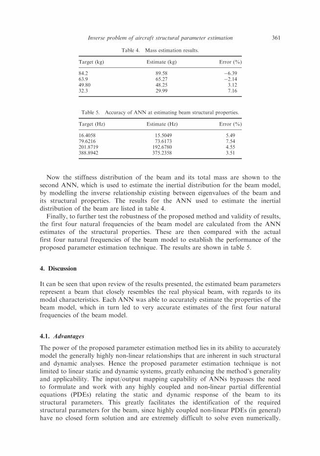
Now the stiffness distribution of the beam and its total mass are shown to thesecond ANN, which is used to estimate the inertial distribution for the beam model,by modelling the inverse relationship existing between eigenvalues of the beam andits structural properties. The results for the ANN used to estimate the inertialdistribution of the beam are listed in table 4.

Finally, to further test the robustness of the proposed method and validity of results,the first four natural frequencies of the beam model are calculated from the ANNestimates of the structural properties. These are then compared with the actualfirst four natural frequencies of the beam model to establish the performance of theproposed parameter estimation technique. The results are shown in table 5.

4. Discussion

It can be seen that upon review of the results presented, the estimated beam parametersrepresent a beam that closely resembles the real physical beam, with regards to itsmodal characteristics. Each ANN was able to accurately estimate the properties of thebeam model, which in turn led to very accurate estimates of the first four naturalfrequencies of the beam model.

4.1. Advantages

The power of the proposed parameter estimation method lies in its ability to accuratelymodel the generally highly non-linear relationships that are inherent in such structuraland dynamic analyses. Hence the proposed parameter estimation technique is notlimited to linear static and dynamic systems, greatly enhancing the method’s generalityand applicability. The input/output mapping capability of ANNs bypasses the needto formulate and work with any highly coupled and non-linear partial differentialequations (PDEs) relating the static and dynamic response of the beam to itsstructural parameters. This greatly facilitates the identification of the requiredstructural parameters for the beam, since highly coupled non-linear PDEs (in general)have no closed form solution and are extremely difficult to solve even numerically.

Table 4. Mass estimation results.

Target (kg) Estimate (kg) Error (%)

84.2 89.58 �6.3963.9 65.27 �2.1449.80 48.25 3.1232.3 29.99 7.16

Table 5. Accuracy of ANN at estimating beam structural properties.

Target (Hz) Estimate (Hz) Error (%)

16.4058 15.5049 5.4979.6216 73.6173 7.54201.8719 192.6780 4.55388.8942 375.2358 3.51


It is indeed the task of each ANN to approximate such equations, which they inherentlydo in an extremely efficient and accurate manner by learning how the static anddynamic response of the beam relates to the structural parameters of the beam duringthe training process.

4.2. Disadvantages

The main limitation of the proposed parameter estimation method is its heavy relianceon the existence of a significant amount of mechanical data (experimental or numerical)pertaining to the type of structure to be identified. The response of the beam structureto some known static loading regime, as well as the free vibratory characteristics ofthe structure must be known in advance. This data must be also be converted such thatit is suitable for use with a simple FEM which, depending on the initial form of thedata, may require significant post-processing.

An additional limitation of the proposed parameter estimation method is the useof relatively few beam finite elements in the beam model to represent the aircraft wing.It is well known that by increasing the number of elements used to model the beam, theaccuracy of results obtained from the finite element analysis will (to a point) increase,particularly for dynamic analyses. In this case, a small number of elements were usedin order to strike a compromise between computational accuracy and efficientimplementation of the ANNs. Using more beam elements in the method will requiremore training and testing data, more hidden layer neurons and longer training times.

Most important, however, is the increased computational expense (longer CPUtime and increased memory requirement) that accompanies an increase in the numberof beam elements used to represent the real beam. For greater than four beam elements,the computational expense of the method becomes overwhelming, while the resultingstructural parameter estimates become less accurate, as compared to the four-elementbeam representation of the physical structure. Hence, the use of four Hermitian beamelements in the beam model was identified as providing the most accurate structuralparameter estimates for a modest computational cost.

Similarly, since the task at hand was to determine the structural parameters of thebeam from a relatively small amount of data regarding its load/deformation and modalcharacteristics, the simple beam model used in the parameter identification proceduremay not be totally representative of the physical structure. Hence, the results achievedmust be considered in the light of the numerous assumptions made regarding theloading regime, boundary conditions and geometry of the aircraft wing.

It is therefore apparent that the proposed parameter estimation method can beimproved in many ways from the discussion so for. Further sophistication of the beammodel accompanied with more physical data for the real aircraft wing will lead to moreaccurate and realistic results. Further, post processing of current available real data maylead to an increase in useful data that the proposed estimation technique can employ.

5. Conclusions

The inertial and bending stiffness distributions of a cantilevered finite element planarbeam were accurately estimated using the proposed hybrid FEM–ANN parameterestimation technique. This simple beam model is capable of small deflections and


rotations and is treated as a simplified representation of an aircraft wing. The stiffness

distribution is estimated from static load/deformation considerations, while the inertial

distribution is estimated from the modal characteristics of the beam model. The results

from the implementation of this proposed parameter estimation technique show that

the estimated parameters produce a beam that has modal characteristics that closely

resemble those of the real physical beam. The proposed parameter estimation method

showed proficiency at modelling the highly non-linear relationships between input

parameters and desired outputs. However, it is anticipated that further refinement

of the beam model will eventually lead to a model that is more representative of the

real structure, for which more accurate results may be obtained.

Acknowledgements

The authors would like to acknowledge the support of the DSTO/RMIT Center

of Expertise in Aerodynamic Loading (CoE-AL), School of Aerospace, Mechanical &

Manufacturing Engineering, RMIT University and the Department of Mechanical and

Aerospace Engineering, University of Texas at Arlington.

References

[1] Gilbert, T. and Trivailo, P.M., 2001, Comparison of manoeuvre strains from non-linear co-rotationalfinite element model of an aircraft wing with flight test data, presented at the 9th Australian InternationalAerospace Congress, Canberra, ACT, Australia.

[2] Dunn, S.A., 1976, Technique for Unique Optimization of Dynamic Finite Element Models (New York:Academic Press).

[3] Levin, A.J. and Levin, R.I., 1998, Dynamic finite element model updating using neural networks.Journal of Vibration and Sound, 210(5), 593–607.

[4] Lee, U., 1995, Equivalent dynamic beam-rod models of aircraft wing structures. Aeronautical Journal,2088, 450–457.

[5] Livne, E. and Navarro, I., 1999, Non-linear equivalent plate modelling of wing-box structures.Journal of Aircraft, 36(5), 851–865.

[6] Kapania, R.K. and Liu, Y., 2001, Equivalent skin analysis of wing structures using neural networks.AIAA Journal, 39(7), 1390–1399.

[7] Haykin, S.S., 1999, Neural Networks: A Comprehensive Foundation (New Jersey: Prentice Hall).[8] Beale, M. and Demuth, H., 2001, Neural Network Toolbox User’s Guide Version 4 (Montana: The Maths

Works Inc.).


Documents

Vol. 14, No. 4, June 2006, 351–363