Embed Size (px)
Citation preview
21/04/16 1
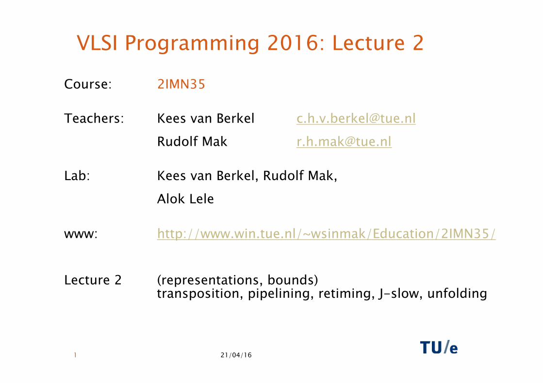
VLSI Programming 2016: Lecture 2
Course: 2IMN35
Teachers: Kees van Berkel [email protected] Rudolf Mak [email protected]
Lab: Kees van Berkel, Rudolf Mak, Alok Lele
www: http://www.win.tue.nl/~wsinmak/Education/2IMN35/ Lecture 2 (representations, bounds)
transposition, pipelining, retiming, J-slow, unfolding
21/04/16 2
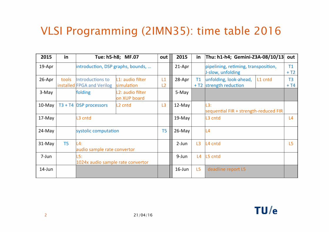
VLSI Programming (2IMN35): time table 2016 2015 in Tue:h5-h8;MF.07 out 2015 in Thu:h1-h4;Gemini-Z3A-08/10/13 out
19-Apr
introduc/on,DSPgraphs,bounds,…
21-Apr
pipelining,re/ming,transposi/on,J-slow,unfolding
T1+T2
26-Apr
toolsinstalled
Introduc/onstoFPGAandVerilog
L1:audiofiltersimula/on
L1L2
28-Apr
T1+T2
unfolding,look-ahead,strengthreduc/on
L1cntd
T3+T4
3-May
folding
L2:audiofilteronXUPboard
5-May
10-May
T3+T4
DSPprocessors
L2cntd
L3
12-May
L3:sequen/alFIR+strength-reducedFIR
17-May
L3cntd
19-May
L3cntd
L4
24-May
systoliccomputa/on
T5
26-May
L4
31-May
T5
L4:audiosamplerateconvertor
2-Jun
L3
L4cntd
L5
7-Jun
L5:1024xaudiosamplerateconvertor
9-Jun
L4
L5cntd
14-Jun
16-Jun
L5
deadlinereportL5
21/04/16 3
Preparation for Lab work
• Prepare your notebook for lab work
• See preparation link on 2IMN35 web-site
• Install the required tools and test them
• First Lab exercises: Tuesday April 26
• Find a partner (team size equals 2)
21/04/16 4
Note on course literature
Lectures VLSI programming are loosely based on: • Keshab K. Parhi. VLSI Digital Signal Processing Systems, Design and
Implementation. Wiley Inter-Science 1999. • This book is recommended, but not mandatory
Accompanying slides can be found on: • http://www.ece.umn.edu/users/parhi/slides.html • http://www.win.tue.nl/~cberkel/2IN35/
Mandatory reading: • Edward A. Lee and David G. Messerschmitt. Synchronous Data
Flow. Proc. of the IEEE, Vol. 75, No. 9, Sept 1987, pp 1235-1245. • Keshab K. Parhi. High-Level Algorithm and Architecture
Transformations for DSP Synthesis. Journal of VLSI Signal Processing, 9, 121-143 (1995), Kluwer Academic Publishers.
21/04/16 5
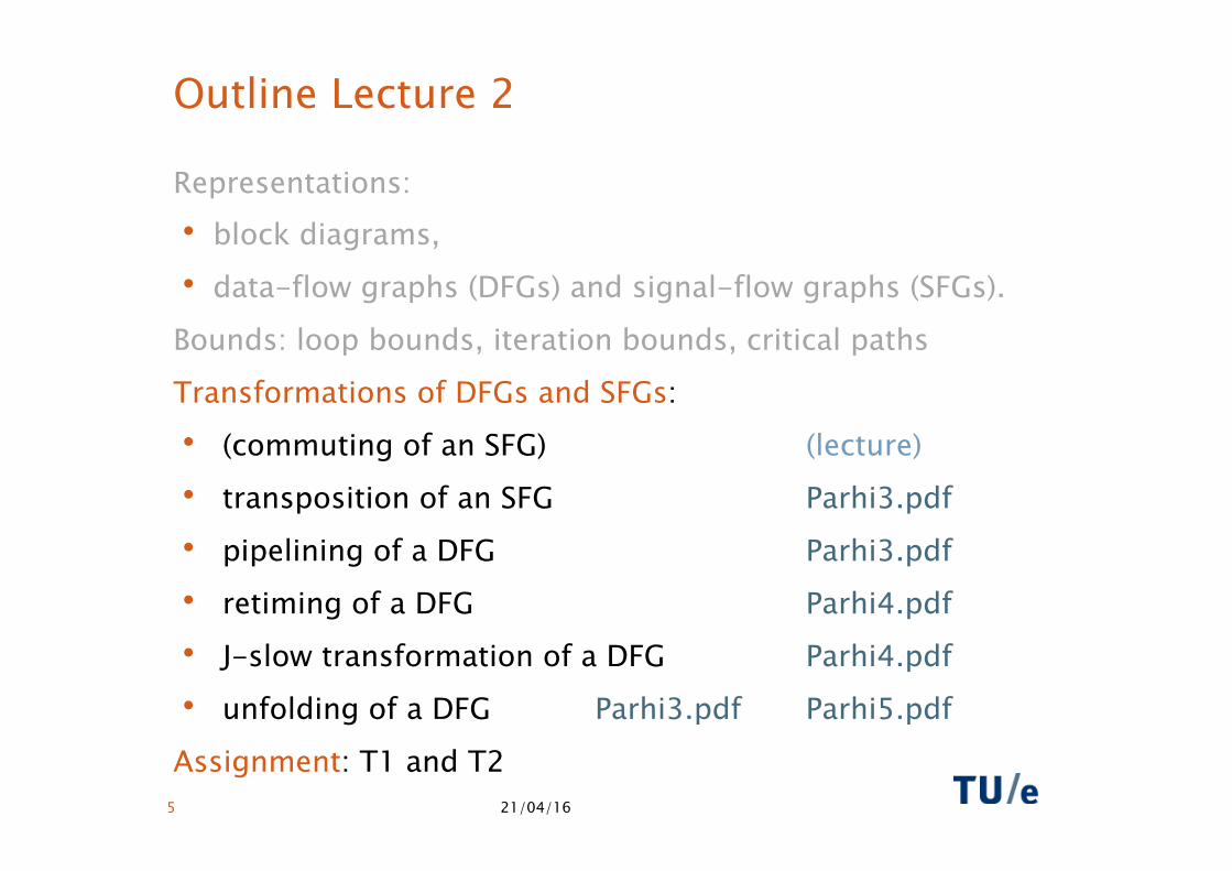
Outline Lecture 2
Representations: • block diagrams, • data-flow graphs (DFGs) and signal-flow graphs (SFGs). Bounds: loop bounds, iteration bounds, critical paths Transformations of DFGs and SFGs: • (commuting of an SFG) (lecture) • transposition of an SFG Parhi3.pdf • pipelining of a DFG Parhi3.pdf • retiming of a DFG Parhi4.pdf • J-slow transformation of a DFG Parhi4.pdf • unfolding of a DFG Parhi3.pdf Parhi5.pdf Assignment: T1 and T2
Parhi
• Note: Many examples and ideas are taken from Parhi’s slides
21/04/16 6
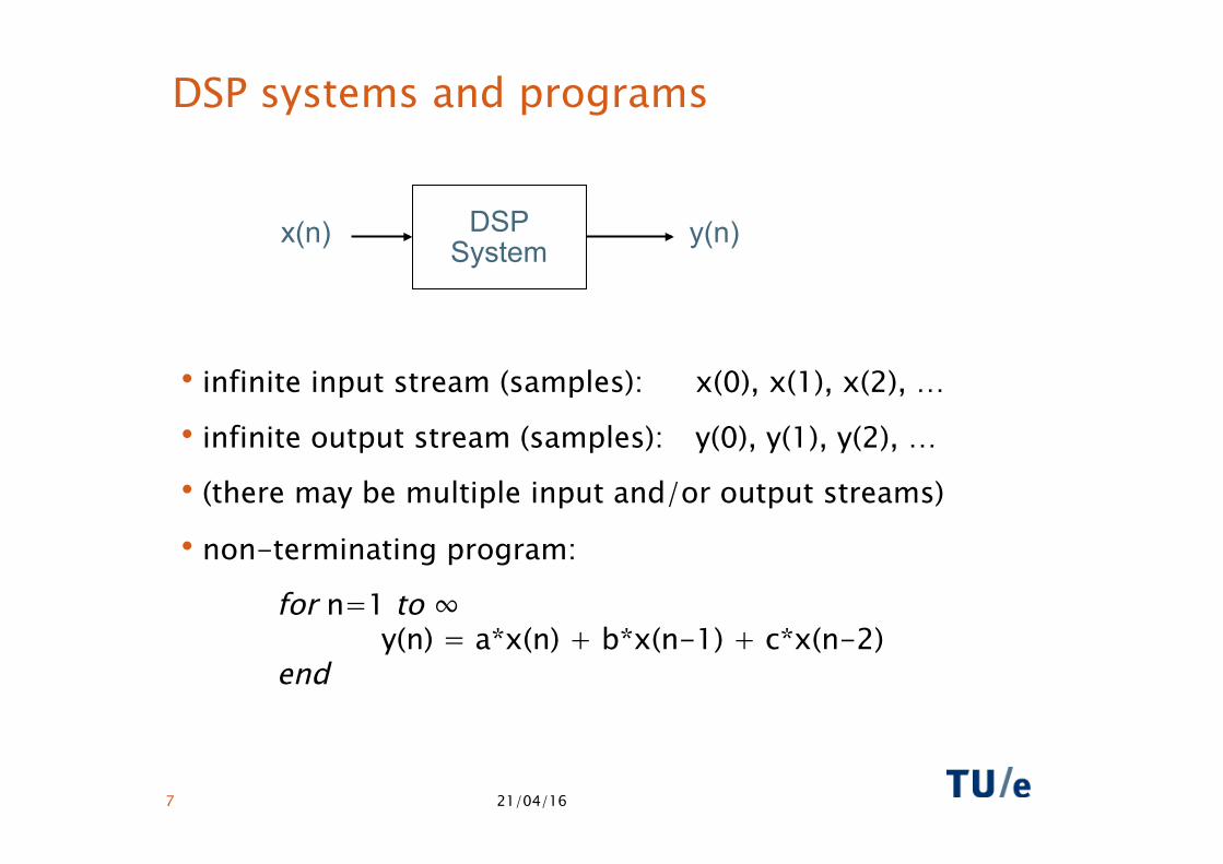
DSP systems and programs
• infinite input stream (samples): x(0), x(1), x(2), …
• infinite output stream (samples): y(0), y(1), y(2), …
• (there may be multiple input and/or output streams)
• non-terminating program:
for n=1 to ∞ y(n) = a*x(n) + b*x(n-1) + c*x(n-2) end
21/04/16 7
DSP System
x(n) y(n)
21/04/16 8
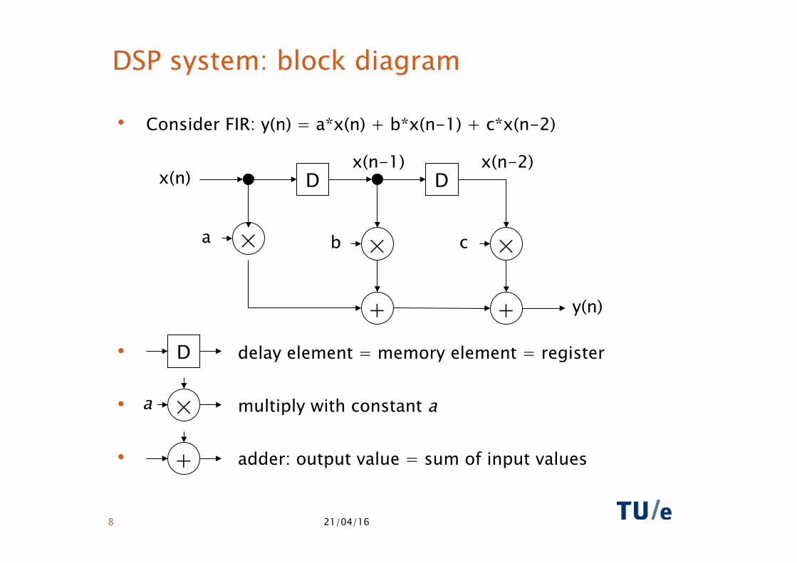
DSP system: block diagram
• Consider FIR: y(n) = a*x(n) + b*x(n-1) + c*x(n-2)
• delay element = memory element = register
• multiply with constant a
• adder: output value = sum of input values
× a × b × c
+ +
D D
y(n)
x(n) x(n-1) x(n-2)
D
× a
+
21/04/16 9
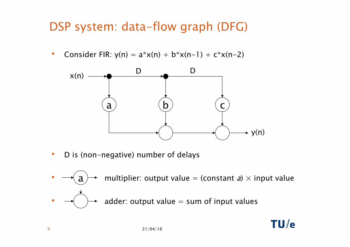
DSP system: data-flow graph (DFG)
• Consider FIR: y(n) = a*x(n) + b*x(n-1) + c*x(n-2)
• D is (non-negative) number of delays
• multiplier: output value = (constant a) × input value
• adder: output value = sum of input values
a b c
y(n)
x(n)
a
D D
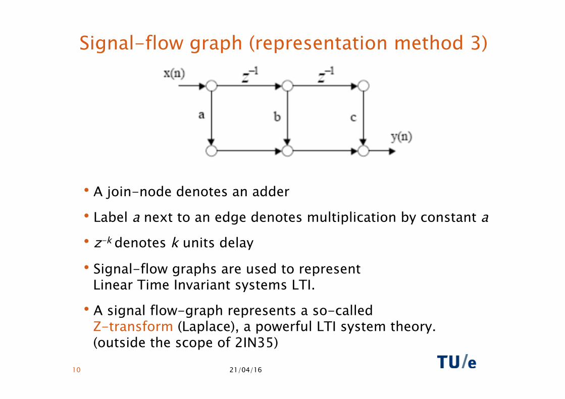
Signal-flow graph (representation method 3)
• A join-node denotes an adder
• Label a next to an edge denotes multiplication by constant a • z-k denotes k units delay
• Signal-flow graphs are used to represent Linear Time Invariant systems LTI.
• A signal flow-graph represents a so-called Z-transform (Laplace), a powerful LTI system theory. (outside the scope of 2IN35)
21/04/16 10
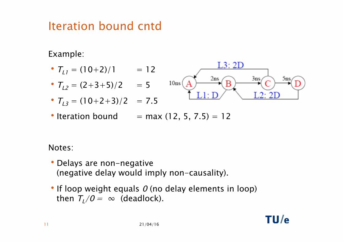
Iteration bound cntd
Example:
• TL1 = (10+2)/1 = 12
• TL2 = (2+3+5)/2 = 5
• TL3 = (10+2+3)/2 = 7.5
• Iteration bound = max (12, 5, 7.5) = 12
Notes:
• Delays are non-negative (negative delay would imply non-causality).
• If loop weight equals 0 (no delay elements in loop) then TL/0 = ∞ (deadlock).
21/04/16 11
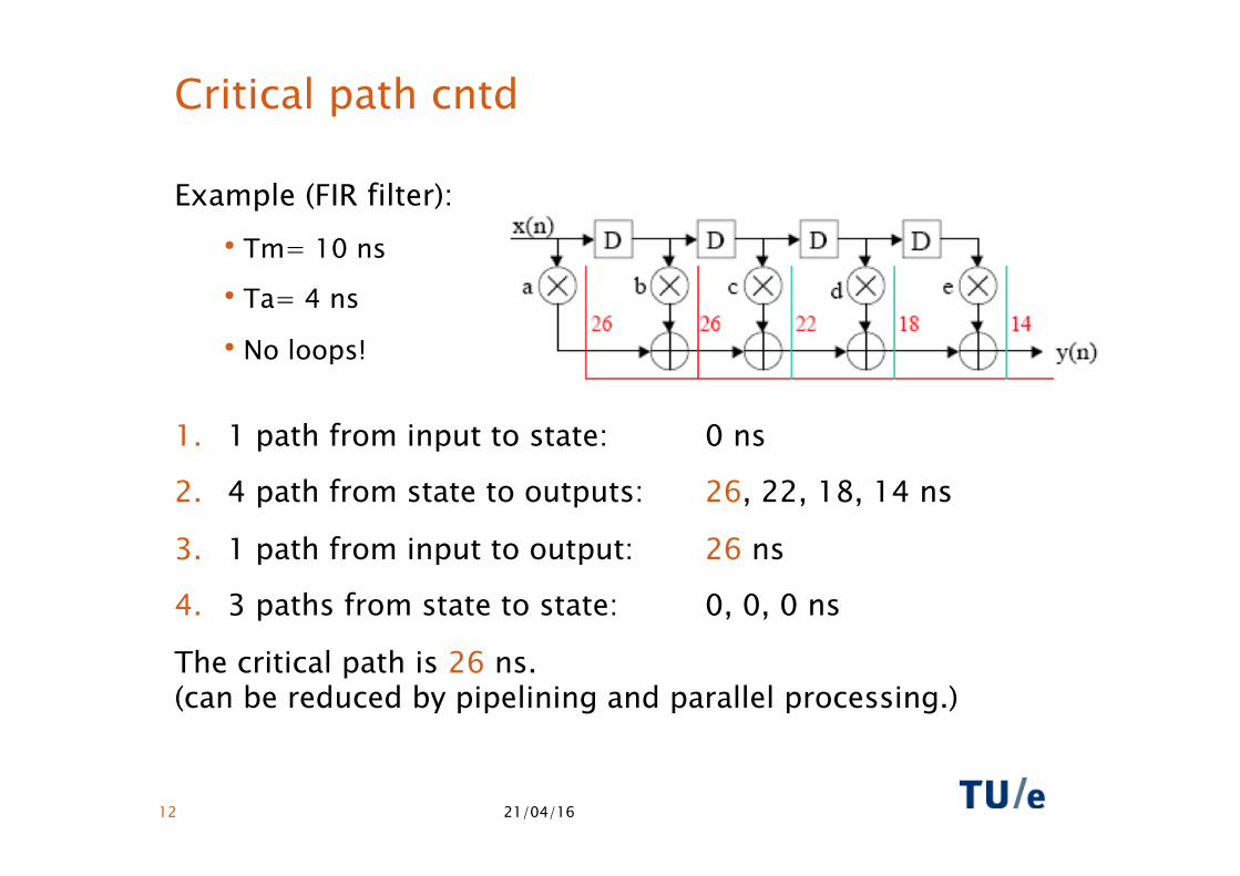
Critical path cntd
Example (FIR filter): • Tm= 10 ns
• Ta= 4 ns
• No loops!
1. 1 path from input to state: 0 ns
2. 4 path from state to outputs: 26, 22, 18, 14 ns
3. 1 path from input to output: 26 ns
4. 3 paths from state to state: 0, 0, 0 ns
The critical path is 26 ns. (can be reduced by pipelining and parallel processing.)
21/04/16 12
TRANSPOSITION OF LTI SYSTEMS
21/04/16 13
21/04/16 14
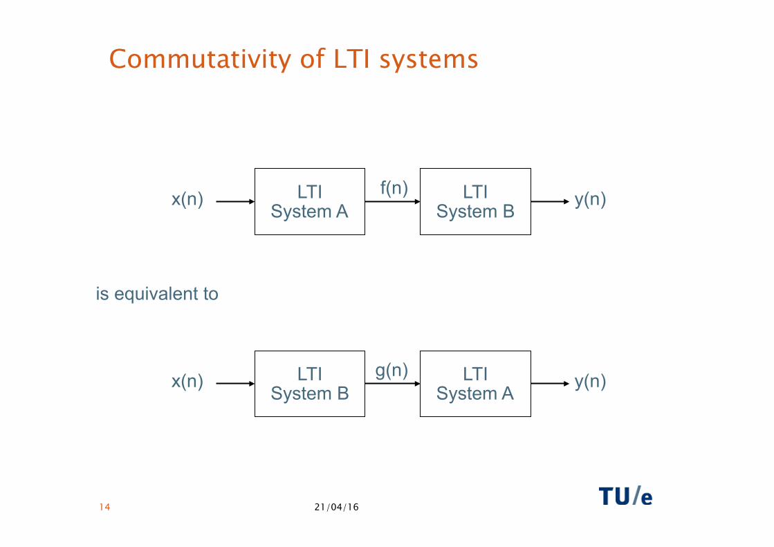
Commutativity of LTI systems
LTI System A
LTI System B
x(n) y(n) f(n)
LTI System B
LTI System A
x(n) y(n) g(n)
is equivalent to

21/04/16 15
Transposition of LTI systems
LTI System A
LTI System B
x(n) y(n) f(n)
LTI System A
LTI System B
y(n) x(n) g(n)
is equivalent to
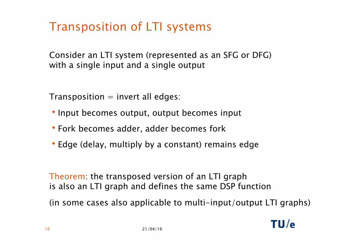
Transposition of LTI systems
Consider an LTI system (represented as an SFG or DFG) with a single input and a single output
Transposition = invert all edges:
• Input becomes output, output becomes input
• Fork becomes adder, adder becomes fork
• Edge (delay, multiply by a constant) remains edge
Theorem: the transposed version of an LTI graph is also an LTI graph and defines the same DSP function
(in some cases also applicable to multi-input/output LTI graphs)
21/04/16 16
21/04/16 17
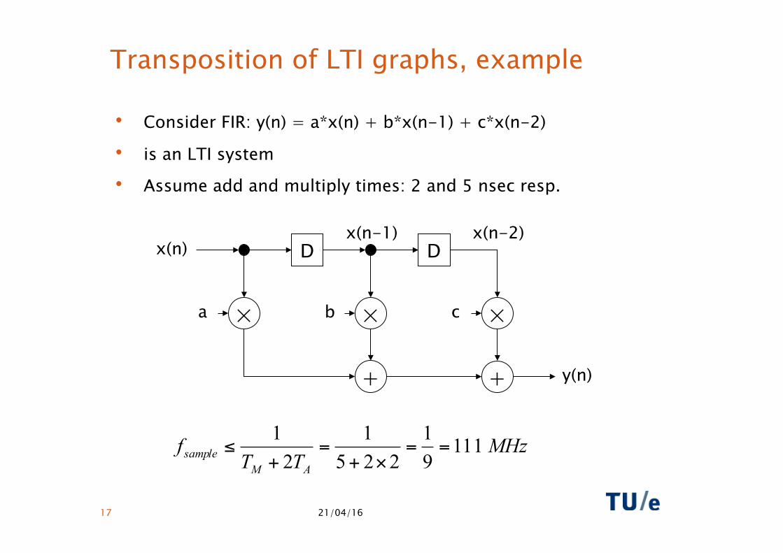
Transposition of LTI graphs, example
• Consider FIR: y(n) = a*x(n) + b*x(n-1) + c*x(n-2)
• is an LTI system
• Assume add and multiply times: 2 and 5 nsec resp.
MHzTT
fAM
sample 11191
2251
21
==×+
=+
≤
× a × b × c
+ +
D D
y(n)
x(n) x(n-1) x(n-2)
21/04/16 18
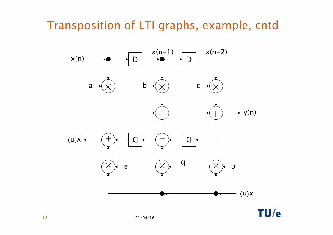
Transposition of LTI graphs, example, cntd
× c × b × a
+ + D D y(n)
x(n)
× a × b × c
+ +
D D
y(n)
x(n) x(n-1) x(n-2)
21/04/16 19
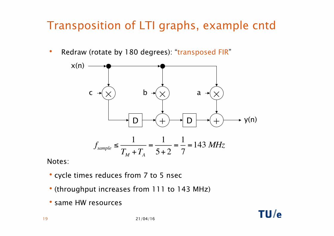
Transposition of LTI graphs, example cntd
• Redraw (rotate by 180 degrees): “transposed FIR”
Notes:
• cycle times reduces from 7 to 5 nsec
• (throughput increases from 111 to 143 MHz)
• same HW resources
fsample ≤1
TM +TA=
15+ 2
=17=143MHz
× c × b × a
+ + D D y(n)
x(n)

PIPELINING
21/04/16 20
Pipeline
An early example of a pipeline is a car assembly line.
[Henry Ford, 1908]. Some 1914 numbers:
• sample time (car parts in / car out): 3 minutes;
• hence, throughput: 20 cars/hour, or approximately 5.5 mHz.
• latency (time between first parts in, car out): 93 minutes;
• number of pipeline stages (stations): 93/3 = 31.
Notes:
• maximum processing time per stage is 3 minutes; some stages may be (much) faster.
• As many as 31 (partial) cars are under assembly.
21/04/16 21
Pipeline
• A pipeline is a chain (cascade) of data-processing elements (“stages”) connected in series (output from one connected to input of next) with a buffer (storage) inserted between these stages.
• Different pipeline stages can operate in parallel, during the same (clock) period.
• The overall throughput is independent of the length of the chain (the number of stages in series).
• The overall throughput is determined by the slowest stage.
Pipelining
• is a transformation that changes the number of stages in a pipeline with the objective to e.g. increase the overall throughput.
• can be applied to block diagrams, DFGs, and SFGs.
21/04/16 22
Pipelining
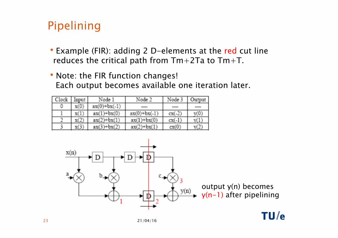
• Example (FIR): adding 2 D-elements at the red cut line reduces the critical path from Tm+2Ta to Tm+T.
• Note: the FIR function changes! Each output becomes available one iteration later.
21/04/16 23
output y(n) becomes y(n-1) after pipelining
Pipelining
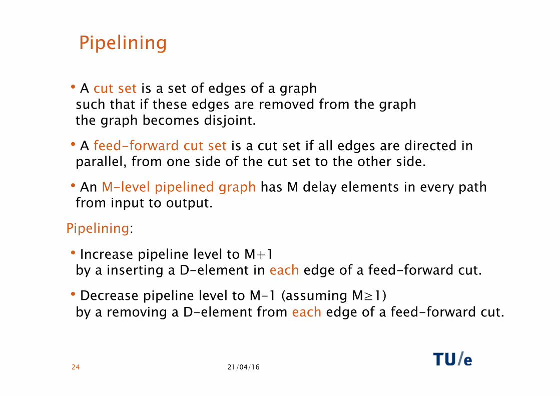
• A cut set is a set of edges of a graphsuch that if these edges are removed from the graphthe graph becomes disjoint.
• A feed-forward cut set is a cut set if all edges are directed in parallel, from one side of the cut set to the other side.
• An M-level pipelined graph has M delay elements in every path from input to output.
Pipelining:
• Increase pipeline level to M+1 by a inserting a D-element in each edge of a feed-forward cut.
• Decrease pipeline level to M-1 (assuming M≥1) by a removing a D-element from each edge of a feed-forward cut.
21/04/16 24
21/04/16 25
Pipelining a simple FIR filter
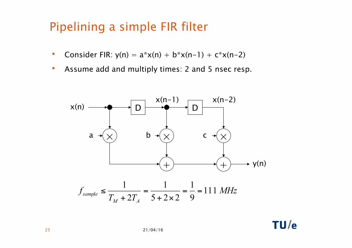
• Consider FIR: y(n) = a*x(n) + b*x(n-1) + c*x(n-2)
• Assume add and multiply times: 2 and 5 nsec resp.
MHzTT
fAM
sample 11191
2251
21
==×+
=+
≤
× a × b × c
+ +
D D
y(n)
x(n) x(n-1) x(n-2)
21/04/16 26
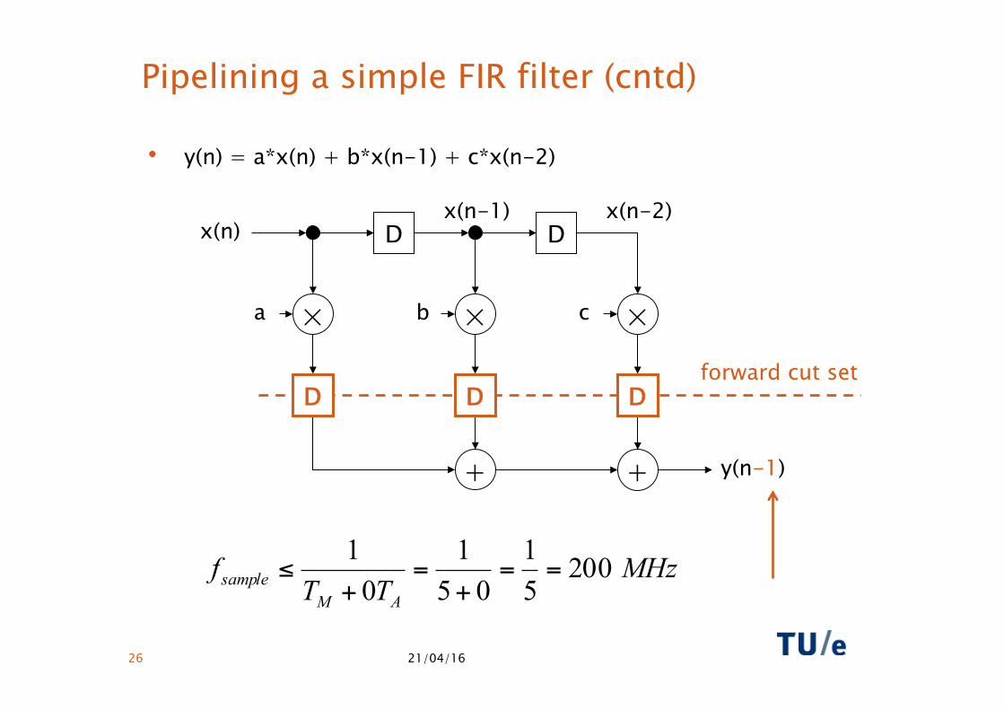
Pipelining a simple FIR filter (cntd)
• y(n) = a*x(n) + b*x(n-1) + c*x(n-2)
MHzTT
fAM
sample 20051
051
01
==+
=+
≤
+ +
D D
y(n-1)
x(n) x(n-1) x(n-2)
× a × b × c
D D D forward cut set
Pipelining/advantages
• Advantage of pipelining: by suitable choosing the feed-forward cut sets, the critical path can be reduced.
• In theory an arbitrary number of pipelines can be inserted, but in practice the added gains (reduced critical path) diminish.
• Note: pipelining can never be used to reduce loop bounds, since graph cycles can not be partitioned by means of a feed-forward cut set.
• Accordingly, pipelining only pays of until the critical path becomes less than the iteration bound.
21/04/16 27
Pipelining/disadvantages
• Disadvantage 1: added D-elements cost additional hardware (latches).
• Disadvantage 2: increased latency. For each added level of pipelining the output(s) become available one iteration (clock period) later.
• Wikipedia: latency is a time interval between the stimulation and response, or, from a more general point of view, as a time delay between the cause and the effect of some physical change in the system being observed.
• added latency [measured in clock cycles] is the added number of pipeline stages due to pipelining.
21/04/16 28
Fine-grained pipelining
• In our course arithmetic nodes (multipliers, adders, …) are considered atomic, with given computation times.
• Implementations of arithmetic nodes are also graphs that can be retimed, down to gate-level (XOR, AND, ..) granularity.
• E.g. it is perfectly possible to find a forward cut set in the graph of a “multiply-by-a-constant” gate-level circuit, such that the circuit is partitioned into two parts with approximately half the computation times each.
• This so-called fine-grained pipelining is a common practice in processor and ASIC (Application Specific IC) design.
• The multipliers offered on the Spartan FPGAs are not pipelined.
21/04/16 29
RETIMING
21/04/16 30
Retiming
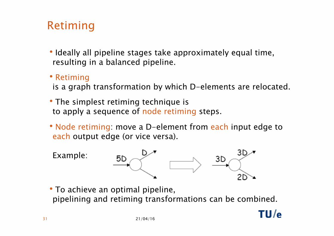
• Ideally all pipeline stages take approximately equal time, resulting in a balanced pipeline.
• Retiming is a graph transformation by which D-elements are relocated.
• The simplest retiming technique is to apply a sequence of node retiming steps.
• Node retiming: move a D-element from each input edge to each output edge (or vice versa). Example:
• To achieve an optimal pipeline, pipelining and retiming transformations can be combined.
21/04/16 31
21/04/16 32
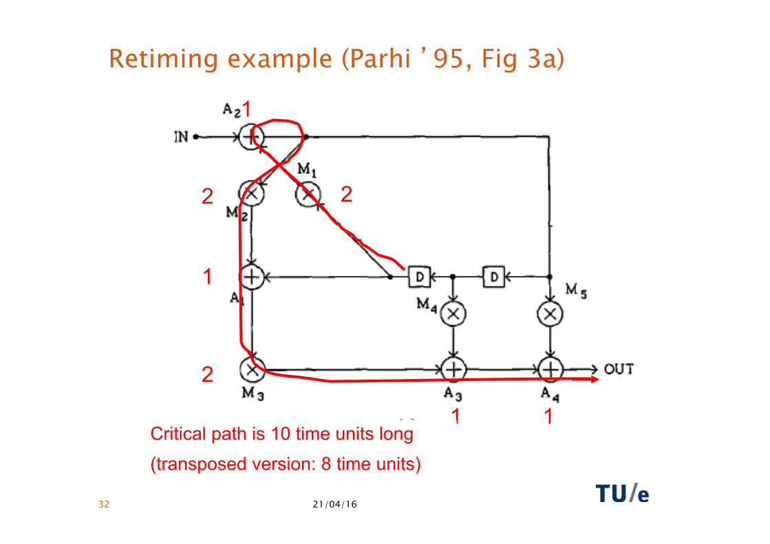
Retiming example (Parhi ’95, Fig 3a)
2
2
2
1
1
1 1 Critical path is 10 time units long (transposed version: 8 time units)
21/04/16 33
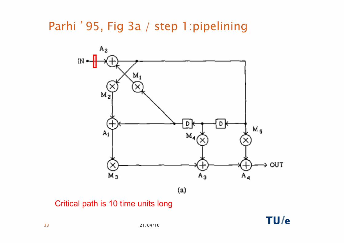
Parhi ’95, Fig 3a / step 1:pipelining
Critical path is 10 time units long
21/04/16 34
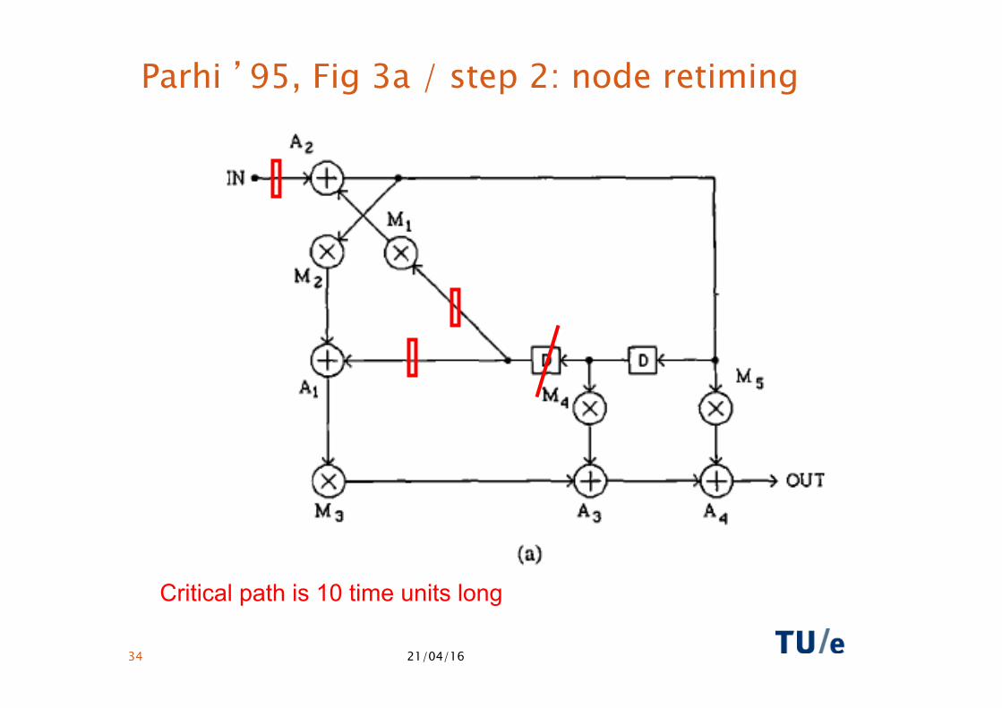
Parhi ’95, Fig 3a / step 2: node retiming
Critical path is 10 time units long
21/04/16 35
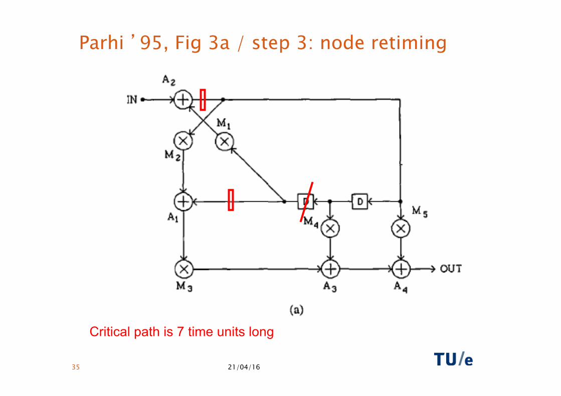
Parhi ’95, Fig 3a / step 3: node retiming
Critical path is 7 time units long
21/04/16 36
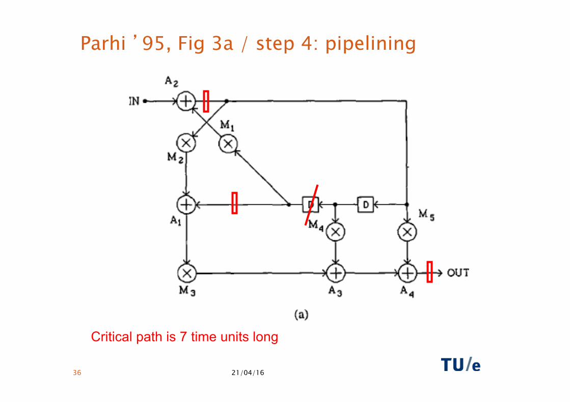
Parhi ’95, Fig 3a / step 4: pipelining
Critical path is 7 time units long
21/04/16 37
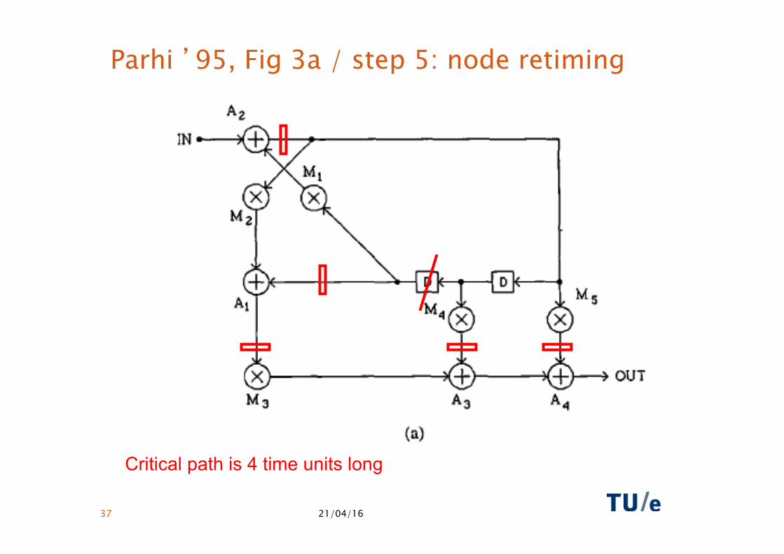
Parhi ’95, Fig 3a / step 5: node retiming
Critical path is 4 time units long
21/04/16 38
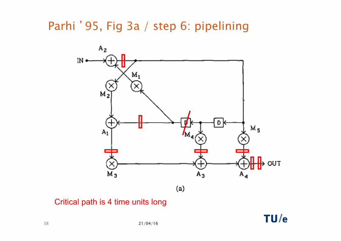
Parhi ’95, Fig 3a / step 6: pipelining
Critical path is 4 time units long
21/04/16 39
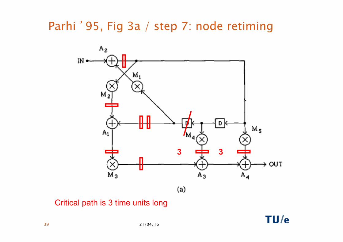
Parhi ’95, Fig 3a / step 7: node retiming
Critical path is 3 time units long
3 3
21/04/16 40
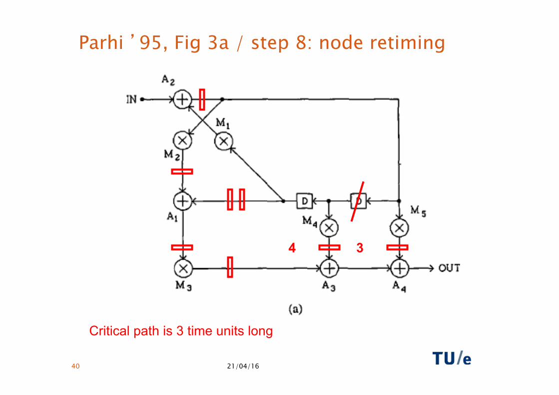
Parhi ’95, Fig 3a / step 8: node retiming
Critical path is 3 time units long
4 3
21/04/16 41
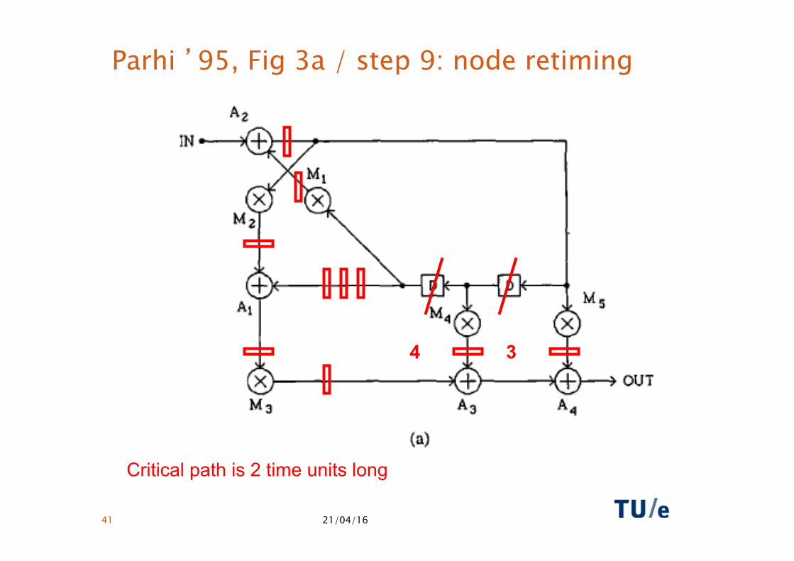
Parhi ’95, Fig 3a / step 9: node retiming
Critical path is 2 time units long
4 3
21/04/16 42
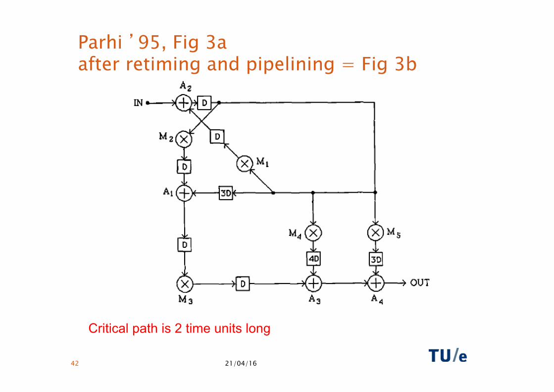
Parhi ’95, Fig 3a after retiming and pipelining = Fig 3b
Critical path is 2 time units long

K-SLOW TRANSFORMATION
21/04/16 43
k-slow transformation
• Replace each D-element by k*D elements.
• This transformation changes the function of the graph.
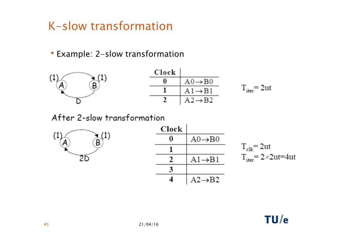
• However, the original function is performed when inputs are offered at clock cycles k*i (i =0,1,2, …) and outputs are consumed during these clock cycles.
• Hence, the hardware is only utilized during 1/k clock cycles
21/04/16 44
K-slow transformation
• Example: 2-slow transformation
21/04/16 45
k-slow transformation
• Benefit 1: the hardware offers the same function during the intermediate clock cycles: k*i+1, k*i+2 … k*i+k-1.
• Example: an stereo audio filter must be performed on the left and right audio channels. Design the filter for one channel, and apply the 2-slow transformation.
• Example: RGB processing for color video.
• Benefit 2: the k-slow transformation increases the number of D-elements in loops (k times), enabling a reduction of critical paths by means of retiming.
21/04/16 46
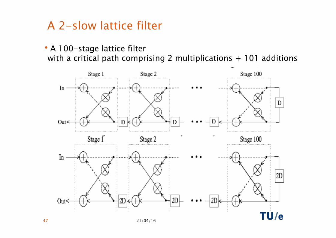
A 2-slow lattice filter
21/04/16 47
• A 100-stage lattice filter with a critical path comprising 2 multiplications + 101 additions
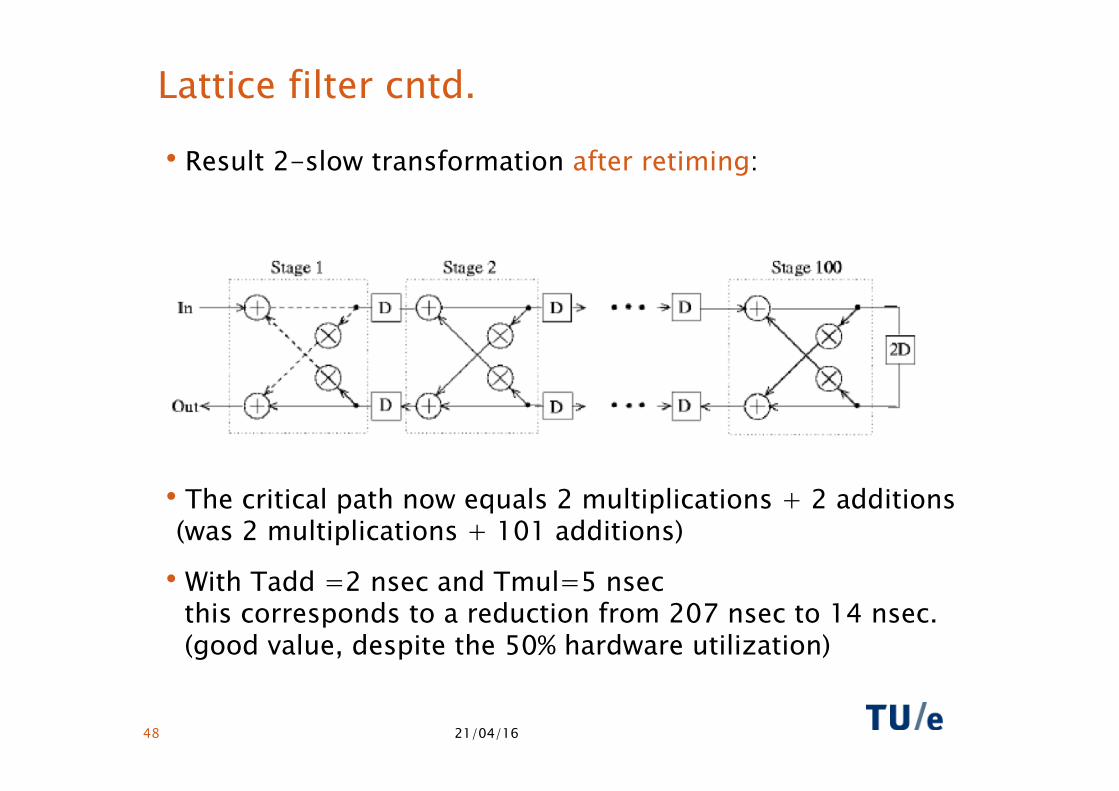
Lattice filter cntd.
• Result 2-slow transformation after retiming:
• The critical path now equals 2 multiplications + 2 additions(was 2 multiplications + 101 additions)
• With Tadd =2 nsec and Tmul=5 nsec this corresponds to a reduction from 207 nsec to 14 nsec. (good value, despite the 50% hardware utilization)
21/04/16 48
PARALLEL PROCESSING
21/04/16 49
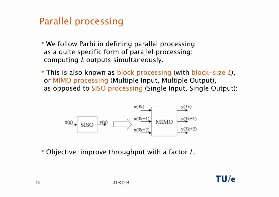
Parallel processing
• We follow Parhi in defining parallel processing as a quite specific form of parallel processing: computing L outputs simultaneously.
• This is also known as block processing (with block-size L), or MIMO processing (Multiple Input, Multiple Output), as opposed to SISO processing (Single Input, Single Output):
• Objective: improve throughput with a factor L.
21/04/16 50
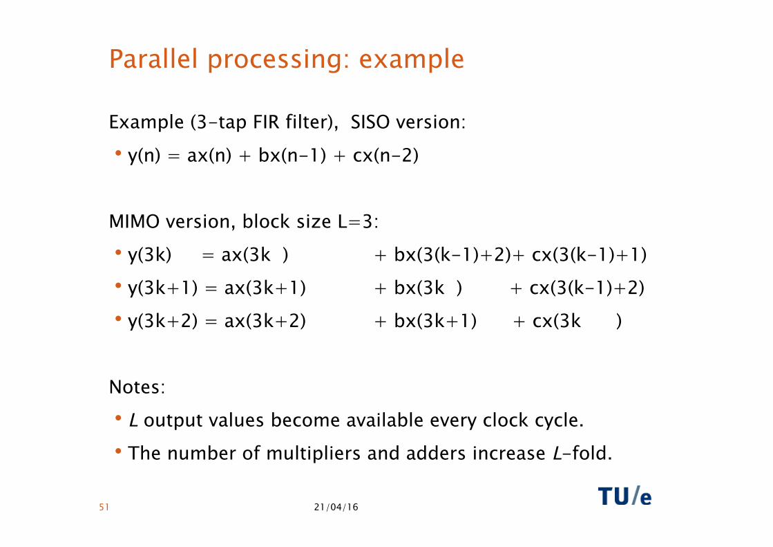
Parallel processing: example
Example (3-tap FIR filter), SISO version: • y(n) = ax(n) + bx(n-1) + cx(n-2) MIMO version, block size L=3: • y(3k) = ax(3k ) + bx(3(k-1)+2)+ cx(3(k-1)+1) • y(3k+1) = ax(3k+1) + bx(3k ) + cx(3(k-1)+2) • y(3k+2) = ax(3k+2) + bx(3k+1) + cx(3k )
Notes: • L output values become available every clock cycle. • The number of multipliers and adders increase L-fold.
21/04/16 51
21/04/16 52
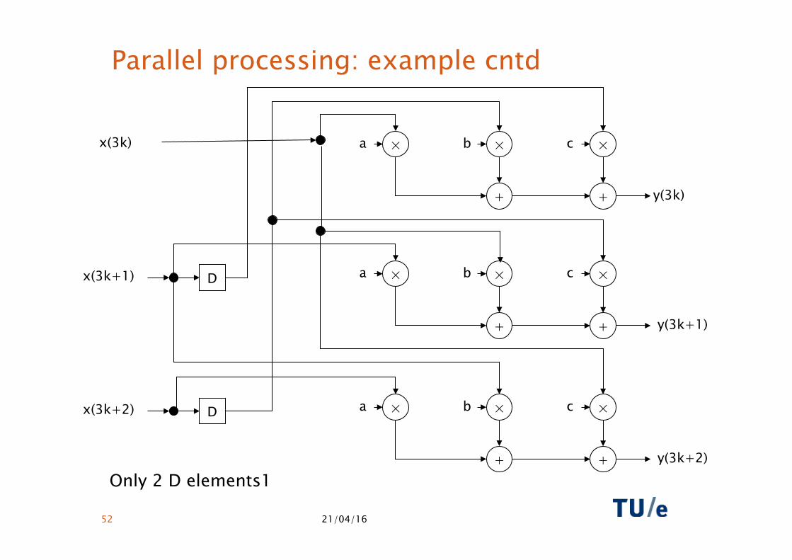
Parallel processing: example cntd
x(3k) × a × b × c
+ + y(3k)
x(3k+1) × a × b × c
+ + y(3k+1)
x(3k+2) × a × b × c
+ + y(3k+2)
D
D
Only 2 D elements1
Parallel processing
• A MIMO implementation (block size L) can be obtained from a SISO implementation by means of L-unfolding.
• Pipelining and unfolding are “dual” techniques (Parhi): if one can be applied (with benefit), so can the other.
• Costs and benefits of pipelining and unfolding differ; often the best result is obtained by applying a combination of both.
21/04/16 53
21/04/16 54
x(2(k-1))
x(10(k-1))
21/04/16 55
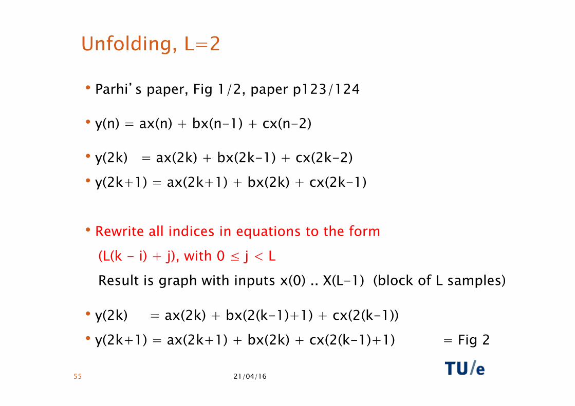
Unfolding, L=2
• Parhi’s paper, Fig 1/2, paper p123/124
• y(n) = ax(n) + bx(n-1) + cx(n-2)
• y(2k) = ax(2k) + bx(2k-1) + cx(2k-2) • y(2k+1) = ax(2k+1) + bx(2k) + cx(2k-1)
• Rewrite all indices in equations to the form (L(k - i) + j), with 0 ≤ j < L Result is graph with inputs x(0) .. X(L-1) (block of L samples)
• y(2k) = ax(2k) + bx(2(k-1)+1) + cx(2(k-1)) • y(2k+1) = ax(2k+1) + bx(2k) + cx(2(k-1)+1) = Fig 2
21/04/16 56
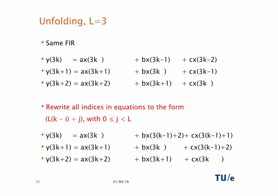
Unfolding, L=3
• Same FIR
• y(3k) = ax(3k ) + bx(3k-1) + cx(3k-2) • y(3k+1) = ax(3k+1) + bx(3k ) + cx(3k-1) • y(3k+2) = ax(3k+2) + bx(3k+1) + cx(3k )
• Rewrite all indices in equations to the form (L(k - i) + j), with 0 ≤ j < L
• y(3k) = ax(3k ) + bx(3(k-1)+2)+ cx(3(k-1)+1) • y(3k+1) = ax(3k+1) + bx(3k ) + cx(3(k-1)+2) • y(3k+2) = ax(3k+2) + bx(3k+1) + cx(3k )

21/04/16 57
Parallel processing: example cntd
x(3k) × a × b × c
+ + y(3k)
x(3k+1) × a × b × c
+ + y(3k+1)
x(3k+2) × a × b × c
+ + y(3k+2)
D
D
Only 2 D elements1
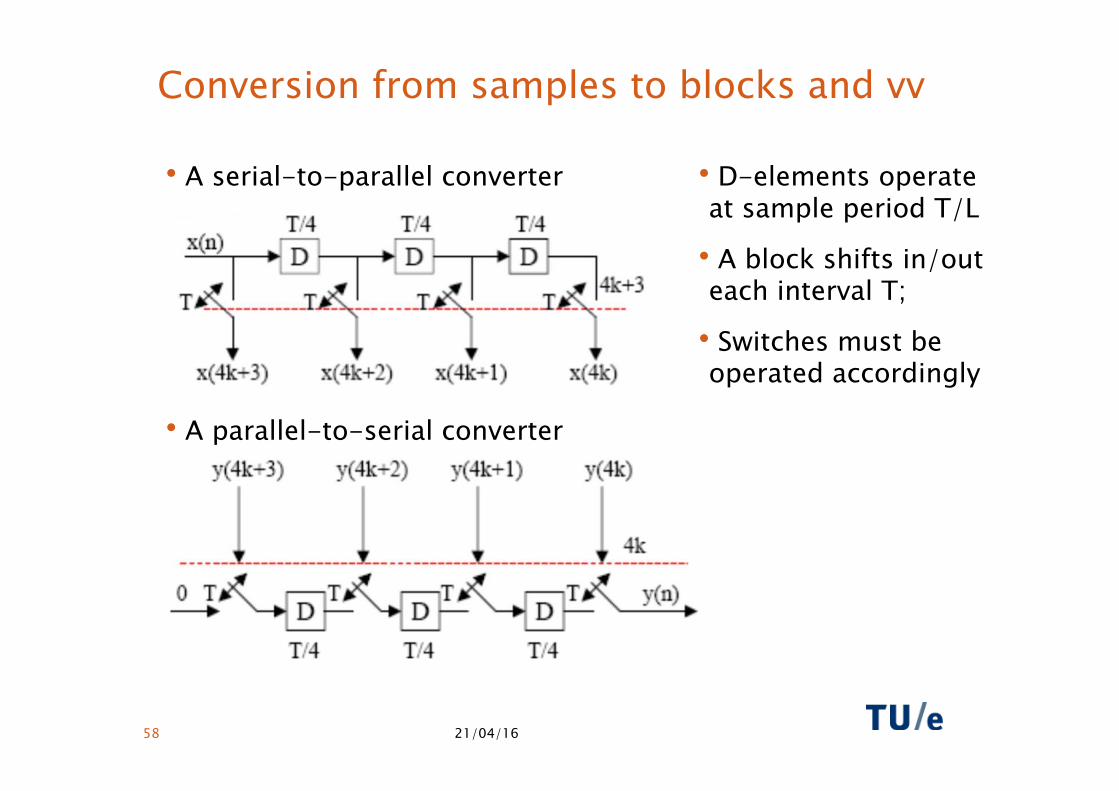
Conversion from samples to blocks and vv
• A serial-to-parallel converter
• A parallel-to-serial converter
• D-elements operate at sample period T/L
• A block shifts in/out each interval T;
• Switches must be operated accordingly
21/04/16 58
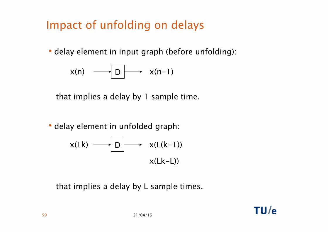
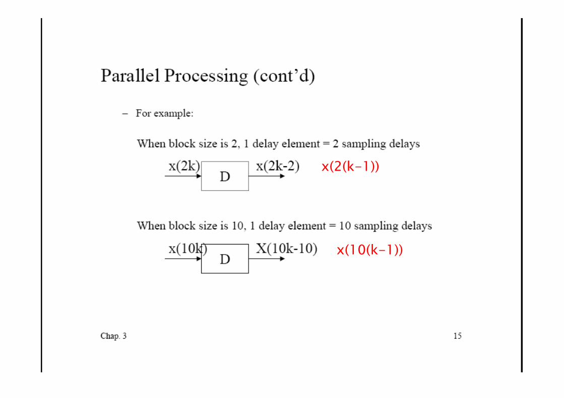
Impact of unfolding on delays
• delay element in input graph (before unfolding):
that implies a delay by 1 sample time.
• delay element in unfolded graph:
that implies a delay by L sample times.
21/04/16 59
D x(n) x(n-1)
D x(Lk) x(L(k-1))
x(Lk-L))
21/04/16 60
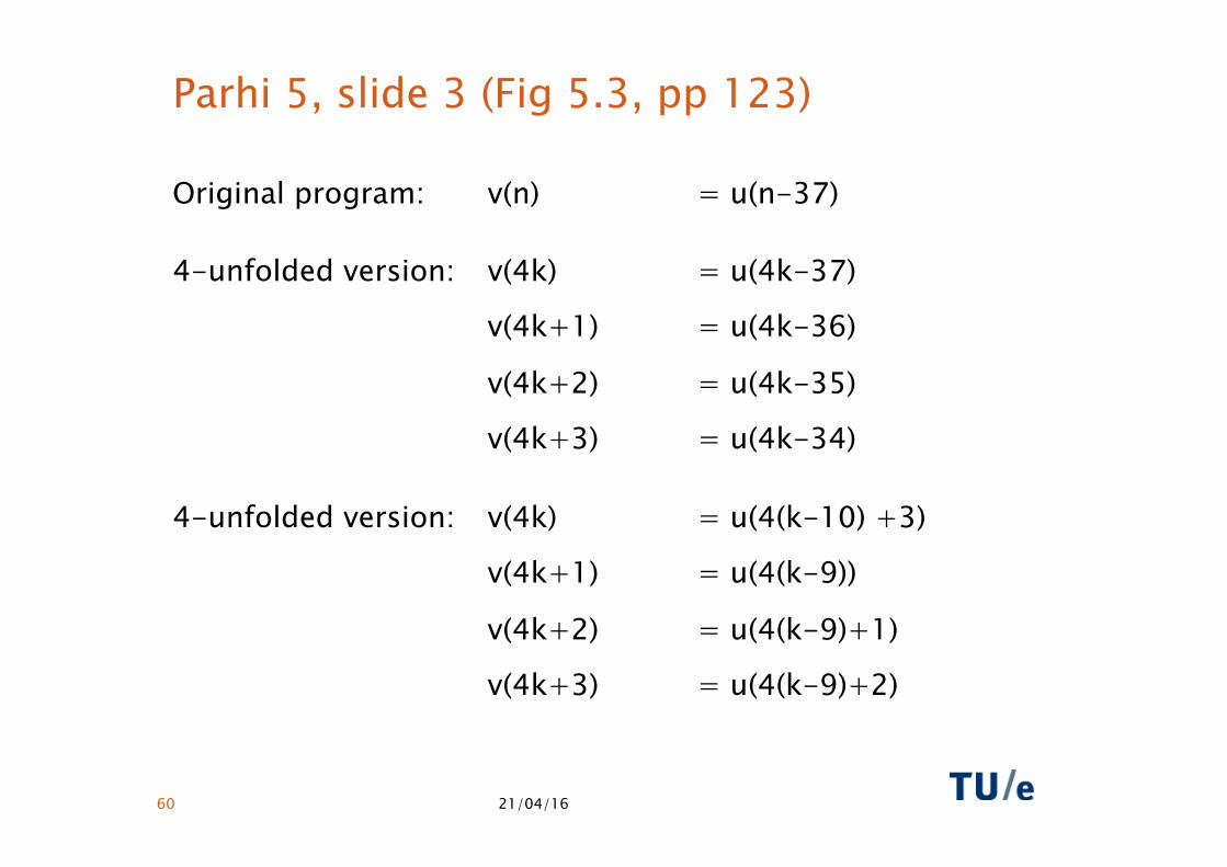
Parhi 5, slide 3 (Fig 5.3, pp 123)
Original program: v(n) = u(n-37)
4-unfolded version: v(4k) = u(4k-37)
v(4k+1) = u(4k-36)
v(4k+2) = u(4k-35)
v(4k+3) = u(4k-34)
4-unfolded version: v(4k) = u(4(k-10) +3)
v(4k+1) = u(4(k-9))
v(4k+2) = u(4(k-9)+1)
v(4k+3) = u(4(k-9)+2)
ASSIGNMENTS T1 AND T2
21/04/16 61
21/04/16 62
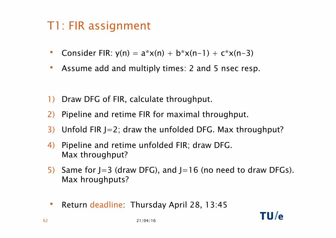
T1: FIR assignment
• Consider FIR: y(n) = a*x(n) + b*x(n-1) + c*x(n-3)
• Assume add and multiply times: 2 and 5 nsec resp.
1) Draw DFG of FIR, calculate throughput.
2) Pipeline and retime FIR for maximal throughput.
3) Unfold FIR J=2; draw the unfolded DFG. Max throughput?
4) Pipeline and retime unfolded FIR; draw DFG. Max throughput?
5) Same for J=3 (draw DFG), and J=16 (no need to draw DFGs). Max hroughputs?
• Return deadline: Thursday April 28, 13:45
21/04/16 63
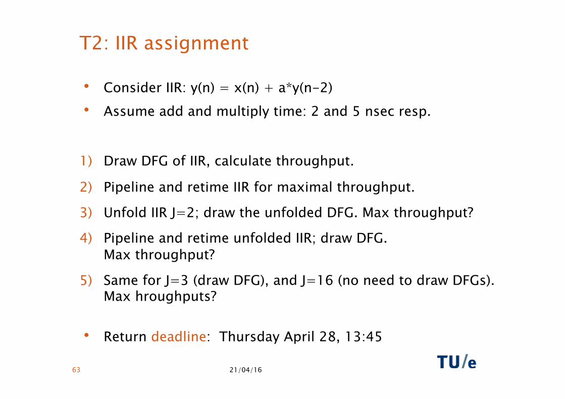
T2: IIR assignment
• Consider IIR: y(n) = x(n) + a*y(n-2) • Assume add and multiply time: 2 and 5 nsec resp.
1) Draw DFG of IIR, calculate throughput.
2) Pipeline and retime IIR for maximal throughput.
3) Unfold IIR J=2; draw the unfolded DFG. Max throughput?
4) Pipeline and retime unfolded IIR; draw DFG. Max throughput?
5) Same for J=3 (draw DFG), and J=16 (no need to draw DFGs). Max hroughputs?
• Return deadline: Thursday April 28, 13:45

THANK YOU