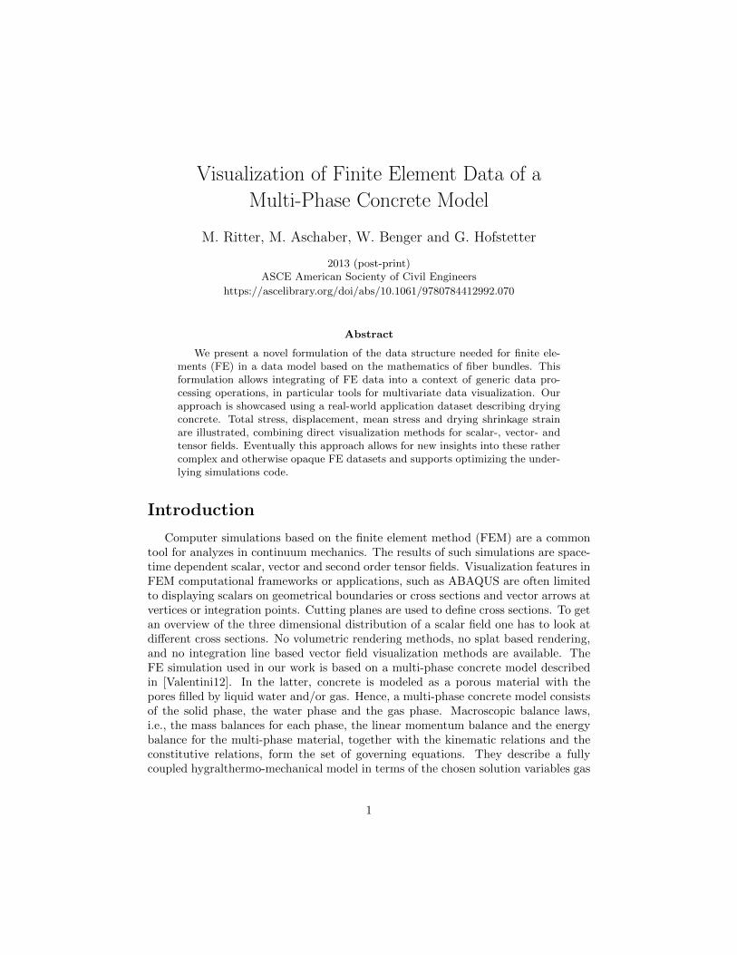
Visualization of Finite Element Data of a

Multi-Phase Concrete Model

M. Ritter, M. Aschaber, W. Benger and G. Hofstetter

2013 (post-print)ASCE American Socienty of Civil Engineers

https://ascelibrary.org/doi/abs/10.1061/9780784412992.070

Abstract

We present a novel formulation of the data structure needed for finite ele-ments (FE) in a data model based on the mathematics of fiber bundles. Thisformulation allows integrating of FE data into a context of generic data pro-cessing operations, in particular tools for multivariate data visualization. Ourapproach is showcased using a real-world application dataset describing dryingconcrete. Total stress, displacement, mean stress and drying shrinkage strainare illustrated, combining direct visualization methods for scalar-, vector- andtensor fields. Eventually this approach allows for new insights into these rathercomplex and otherwise opaque FE datasets and supports optimizing the under-lying simulations code.

Introduction

Computer simulations based on the finite element method (FEM) are a commontool for analyzes in continuum mechanics. The results of such simulations are space-time dependent scalar, vector and second order tensor fields. Visualization features inFEM computational frameworks or applications, such as ABAQUS are often limitedto displaying scalars on geometrical boundaries or cross sections and vector arrows atvertices or integration points. Cutting planes are used to define cross sections. To getan overview of the three dimensional distribution of a scalar field one has to look atdifferent cross sections. No volumetric rendering methods, no splat based rendering,and no integration line based vector field visualization methods are available. TheFE simulation used in our work is based on a multi-phase concrete model describedin [Valentini12]. In the latter, concrete is modeled as a porous material with thepores filled by liquid water and/or gas. Hence, a multi-phase concrete model consistsof the solid phase, the water phase and the gas phase. Macroscopic balance laws,i.e., the mass balances for each phase, the linear momentum balance and the energybalance for the multi-phase material, together with the kinematic relations and theconstitutive relations, form the set of governing equations. They describe a fullycoupled hygralthermo-mechanical model in terms of the chosen solution variables gas

1

pressure, capillary pressure, displacements and temperature. The multi-phase con-crete model has been used particularly to simulate drying shrinkage of concrete in amore realistic way. After the setting of the concrete, commonly, the pore humidityis higher than the ambient relative humidity and, thus, a drying process starts. Thisdrying process decreases the relative pore humidity of concrete and increases the cap-illary pressure, which exerts a hydrostatic pressure on the cement matrix resulting involumetric compaction, known as drying shrinkage.

The visualization of FE data is still an ongoing research area. Early work wasdone on parallel workstation systems, e.g. based on ray-casting [Garrity90] or basedon tetrahedral splatting [Williams92]. Other methods are based on particles, iso-surface or cutting planes. FE data is often re-sampled on uniform grids allowingfast and well studied texture based volume rendering techniques [Engel06]. Here,work was done on multivariate techniques, e.g., [Stompel02] also utilizing non-photorealistic techniques. Modern GPU based direct visualization techniques are usuallybased on ray-casting. [Bock12] was able to shift heavy computational parts into apre-processing step improving the GPU rendering for interactive performance.

However, most approaches are limited to a certain grid type, do not use ad vancedtechniques developed in texture based volume rendering or are not formulated withaspect to multivariate data. We are aiming at usage of a general data model toenable techniques independent of, or applicable to many, grid types. Our data modelis motivated and introduced in the next section F5 Data Model. The modeling of FEdata is presented and data conversion is described. The section Visualization presentsthe utilizes visualization techniques, which are applied in section Visualization of aDrying Concrete Specimen. Finally, a Summary is provided.

F5 Data Model

Motivation. In order to be able to best reuse existing visualization techniques, itis necessary to find most general or common solutions for specific problems. Thecomputational and observational sciences nowadays produce more and more datasetsof different kinds. Data analysis and visualization plays an important role in the un-derstanding and interpretation of datasets. Errors in simulation codes might not bediscovered if not visualized properly. Many different data layouts are used for numer-ical computations dependent on the applied methods and spatio-temporal discretiza-tion: uniform grids, rectilinear grids, curvilinear grids, hexahedral grids, unstructuredgrids, particles, etc. Already in 1989 [Butler89] proposed to use the mathematicalmodel of fiber bundles as a foundation for a common data model. Using such a sys-tematic model enables to apply visualization technique across a wide range of differentdata sources.

Mathematics. The data model utilized in our work is based on the theory of fiberbundles. This models any data as a total space, which is constructed from a so-calledbase space and fiber space. While the base-space corresponds to a manifold, the fiberspace corresponds to data attached to each of the points of the entity. The discretizedbase space describes a finite sampling of data points including their (discrete, integer)neighborhood information, whereas the fiber space usually is continuous, containing

2

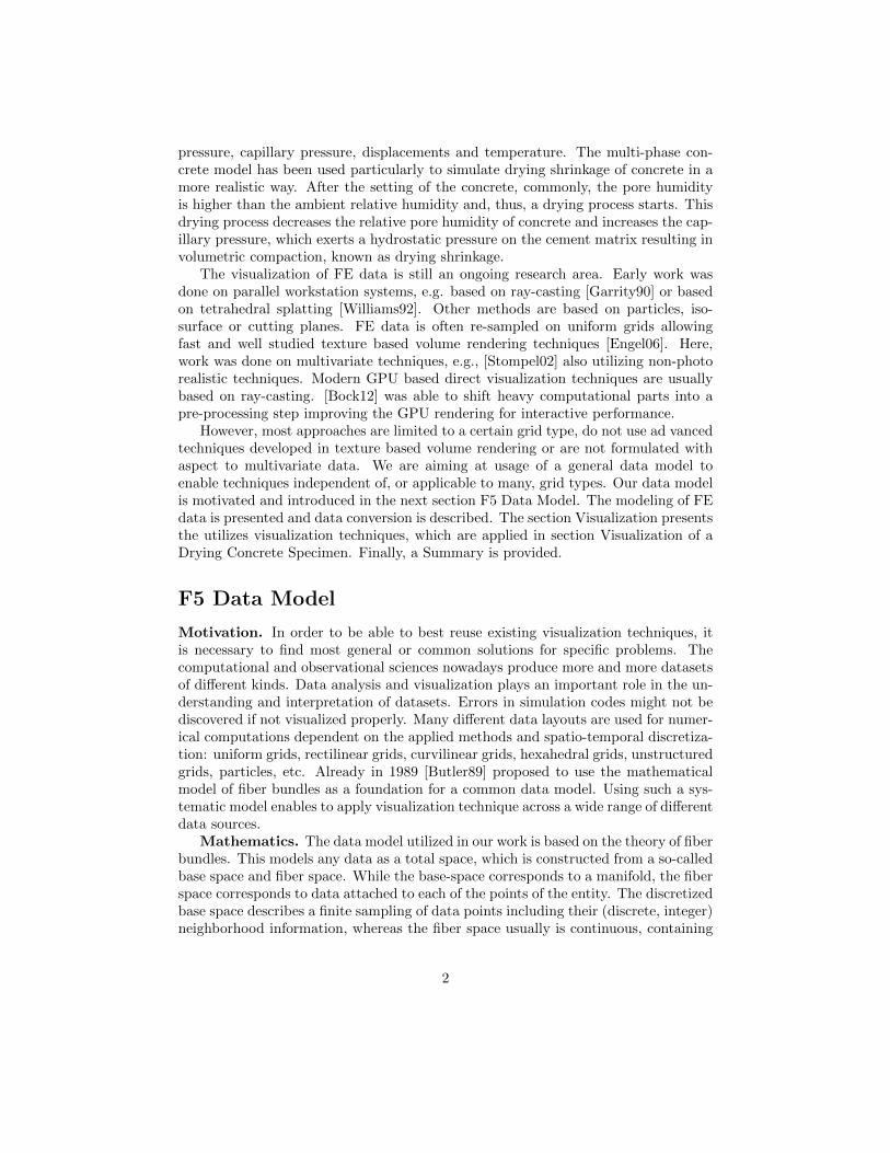
Slice/Grid/Skeleton/Represenation/Field/(Fragment)

SkeletonRepresentation

Field( Fragment)

GridSlice

Figure 1: Hierarchical data organization of the F5 data model.

floating-point data such as scalar, vectorial and tensorial quantities. This data modelsuits very well spatio-temporal data occurring in scientific visualization and coversmost numerical simulations. Data structures used for finite elements add a newproperty to the data though, which are interpolation weights and evaluation points.These are not inherently spatio-temporal, but rather ”supplementary information” asrequired for the numerical simulations. There is no explicit base space associated withthese FE data as they describe information between data points. However, the datamodel used in our work [Ben04] allows to also formulate data given on relationshipsbetween base spaces, properties of a base space (i.e, the skeletons of a CW-complex) and even entirely separate manifolds. This capability serves well to express theproperties of a FE data structure in the existing data model without need to modifythe data model itself, as will be elaborated in the following sections.

Hierarchy. The data model is organized in a hierarchy, see Figure 1. Firstelement is the time level storing time as a double floating point variable, called Slice.Inside a time slice geometric objects are stored, called Grid objects. A grid object isdescribed by at least one topology object, called Skeleton. The properties of a skeletonare defined by the dimensionality of the skeleton (point=0, line=1, surface=2, ...), therefinement level, and the index depth. The index depth is the number of indirectionsto reach the most basic point skeleton. An edge skeleton would have dimensionalityone and index depth one, because an edge is defined as a pair of point indices and,thus, an indirection of one to the points. A line skeleton defined via indices of edgeswould have a dimensionality of one and an index depth of two. Inside a skeletonobject, data can be defined in one or more Representations. Here, certain coordinatesystems can be specified, such as 3D-Cartesian or 3D-Spherical. Representations canalso be specified relative to another skeleton. For example, if an edge is defined viapoint indices, an according representation would be located in the edge skeleton called’EdgeAsPoints’, which indicates that the used indices are those of the point skeleton.Numerical data is stored in the Field. A field is a named data array of (compound)elements, e.g. a three dimensional array of second order tensors. A field called’Positions’ describes the geometry of the skeleton. For example, a ’Positions’ field ina point skeleton stores the coordinates in the Cartesian representation, a ’Positions’field in the edge skeleton stores the point indices in the EgdesAsPoints representation.All the skeletons in combination with their according ’Positions’ fields form the basespace, the manifold, of a grid object. Data fields can be added in any representation

3

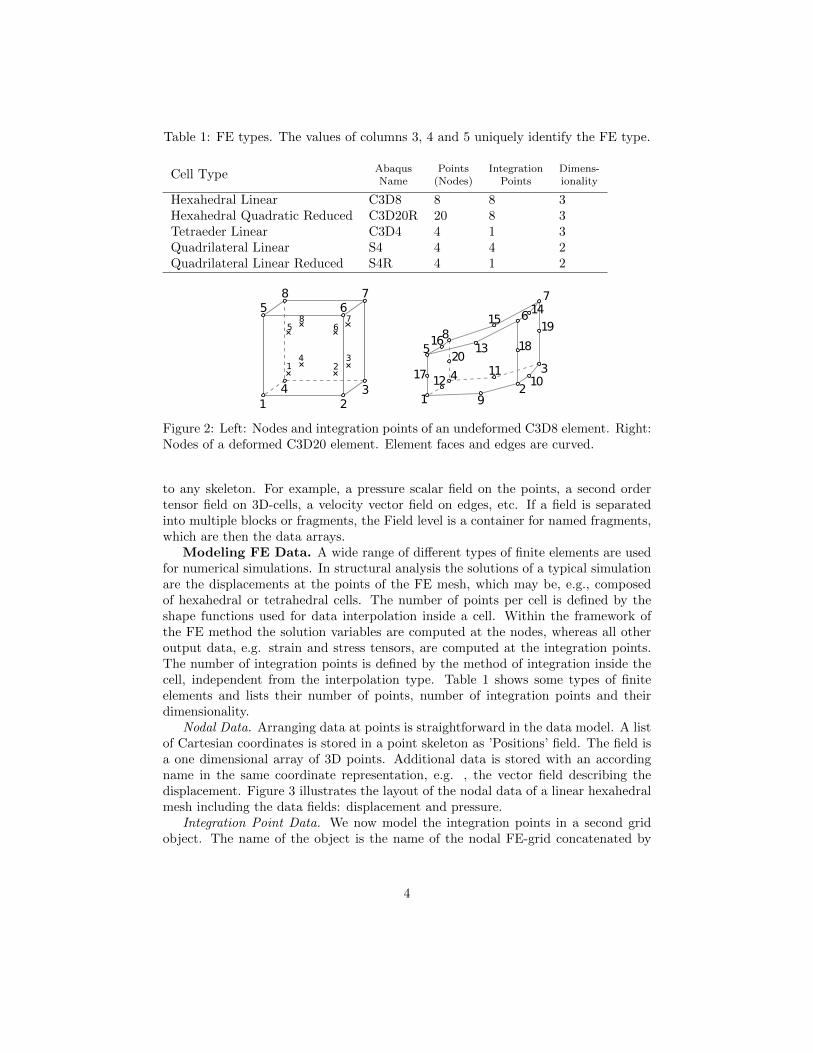
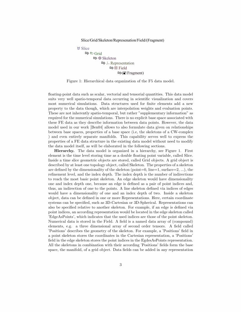
Table 1: FE types. The values of columns 3, 4 and 5 uniquely identify the FE type.

Cell Type AbaqusName

Points(Nodes)

IntegrationPoints

Dimens-ionality

Hexahedral Linear C3D8 8 8 3Hexahedral Quadratic Reduced C3D20R 20 8 3Tetraeder Linear C3D4 4 1 3Quadrilateral Linear S4 4 4 2Quadrilateral Linear Reduced S4R 4 1 2

1 234

5 678

8

1 234

5 67

12

34

5

6

7

8

9

1011

12

13

14

16

17

18

19

20

15

Figure 2: Left: Nodes and integration points of an undeformed C3D8 element. Right:Nodes of a deformed C3D20 element. Element faces and edges are curved.

to any skeleton. For example, a pressure scalar field on the points, a second ordertensor field on 3D-cells, a velocity vector field on edges, etc. If a field is separatedinto multiple blocks or fragments, the Field level is a container for named fragments,which are then the data arrays.

Modeling FE Data. A wide range of different types of finite elements are usedfor numerical simulations. In structural analysis the solutions of a typical simulationare the displacements at the points of the FE mesh, which may be, e.g., composedof hexahedral or tetrahedral cells. The number of points per cell is defined by theshape functions used for data interpolation inside a cell. Within the framework ofthe FE method the solution variables are computed at the nodes, whereas all otheroutput data, e.g. strain and stress tensors, are computed at the integration points.The number of integration points is defined by the method of integration inside thecell, independent from the interpolation type. Table 1 shows some types of finiteelements and lists their number of points, number of integration points and theirdimensionality.

Nodal Data. Arranging data at points is straightforward in the data model. A listof Cartesian coordinates is stored in a point skeleton as ’Positions’ field. The field isa one dimensional array of 3D points. Additional data is stored with an accordingname in the same coordinate representation, e.g. , the vector field describing thedisplacement. Figure 3 illustrates the layout of the nodal data of a linear hexahedralmesh including the data fields: displacement and pressure.

Integration Point Data. We now model the integration points in a second gridobject. The name of the object is the name of the nodal FE-grid concatenated by

4

T=0.0

Positions Indices <8 x unsigned long>

StressAv Tensor <6 x double>( )

StressAv Tensor <8 x <6 x double> >( )

Positions PointDisplacement VectorPressure Scalar

<3 x double><3 x double><double>

FE-MeshPoints

Cartesian

CellsAsPointsCells

Figure 3: F5 layout of a C3D8 element’s nodal data. Data fields displacement andpressure are stored in the ’Points’ skeleton. Cells are defined in another skeleton viaindices to the point ’Positions’ in the relative representation ’CellsAsPoints’.

T=0.0FE-Mesh_IPT=0.0

PointsCartesian

Stress Tensor<6 x double>Cells

CellsAsPointsPositions Indices<8 x unsigned long>

Figure 4: F5 layout of a C3D8 element’s integration point data. One exemplary stressdata field is stored in the ’Points’ skeleton. No ’Points’ ’Positions’ field is required asintegration point coordinates can be computed from the nodal grid.

a standardized postfix. Figure 4 illustrates this second grid. The ’Positions’ field ofthe ’Points’ skeleton is not required, since it can be computed from the nodal pointsand cells. The two ’Cell’ topologies in the two grid object share the same index base:same index for the same cell, thus, relating integration points to nodes and vice versa.

Time Independent Data. Some data fields are time independent. The cell connec-tivities need not be stored in every time slice. Also, the node positions can be staticand current ones can then be computed from the original coordinates and the currentdisplacement vector. In these cases the data field objects are replaced by pointers tothe according fields stored in the first time slice. When working with the hierarchythis data reduction is hidden and the field can be normally accessed at any slice.

Averaged and Cell Relative Nodal Data. For the purpose of visualization, data ismostly requested on nodes because the shape functions require this for data inter-polation. Thus, data given on integration points only, have to be recomputed intorepresentative values at the nodes. This is done in two steps: computation of nodalvalues per cell, and averaging all nodal values per node (arithmetic mean). The percell data set is stored as a data field in the nodal ’CellsAsPoints’ representation. Theaveraged nodal field is stored in the nodal Cartesian points representation. Figure 3illustrates the two computed fields ’StressAv’ in round brackets.

Selection Sets. Sets of elements are used to define properties, such as a materi-

5

PositionsPName1 VLen<V x unsigned long>

Positions

CClusterCClusterAsPoints

CName1 VLen<V x unsigned long>CName2 VLen<V x unsigned long>

T=0.0FE-Mesh

PClusterPClusterAsPoints

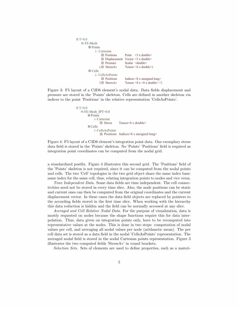
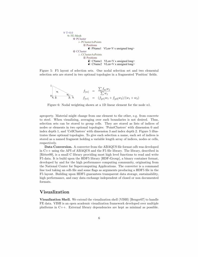
Figure 5: F5 layout of selection sets. One nodal selection set and two elementalselection sets are stored in two optional topologies in a fragmented ’Position’ fields.

1

0n1 n2p1 p2

ww

1

2

f[ni] =

∑fpjwj∑wj

f[n1] = (f[p1]w1 + f[p2]w2)/(w1 + w2)

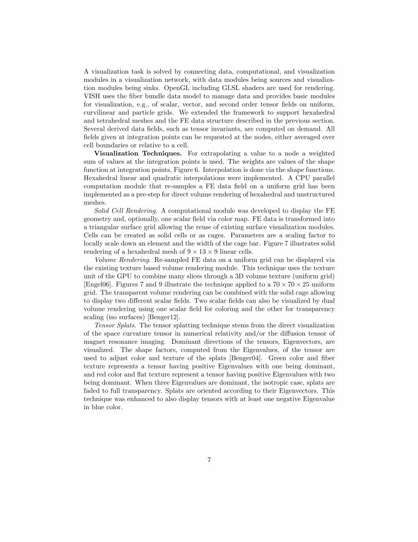
Figure 6: Nodal weighting shown at a 1D linear element for the node n1.

aproperty. Material might change from one element to the other, e.g. from concreteto steel. When visualizing, averaging over such boundaries is not desired. Thus,selection sets can be stored to group cells. They are stored as lists of indices ofnodes or elements in two optional topologies: ’PointClusters’ with dimension 0 andindex depth 1, and ’CellClusters’ with dimension 3 and index depth 2. Figure 5 illus-trates these optional topologies. To give each selection a name, each set of indices isstored as a named fragment holding a variable length array of indices, nodes or cells,respectively.

Data Conversion. A converter from the ABAQUS file format odb was developedin C++ using the API of ABAQUS and the F5 file library. The library, described in[Ritter09], is a small C library providing most high level functions to read and writeF5 data. It is build upon the HDF5 library [HDF-Group], a binary container format,developed by and for the high performance computing community, originating fromthe National Center for Supercomputing Applications. The converter is a commandline tool taking an odb file and some flags as arguments producing a HDF5 file in theF5 layout. Building upon HDF5 guarantees transparent data storage, sustainability,high performance, and easy data exchange independent of closed or non documentedformats.

Visualization

Visualization Shell. We extend the visualization shell (VISH) [Benger07] to handleFE data. VISH is an open academic visualization framework developed over multipleplatforms in C++. External library dependencies are kept as minimal as possible.

6

A visualization task is solved by connecting data, computational, and visualizationmodules in a visualization network, with data modules being sources and visualiza-tion modules being sinks. OpenGL including GLSL shaders are used for rendering.VISH uses the fiber bundle data model to manage data and provides basic modulesfor visualization, e.g., of scalar, vector, and second order tensor fields on uniform,curvilinear and particle grids. We extended the framework to support hexahedraland tetrahedral meshes and the FE data structure described in the previous section.Several derived data fields, such as tensor invariants, are computed on demand. Allfields given at integration points can be requested at the nodes, either averaged overcell boundaries or relative to a cell.

Visualization Techniques. For extrapolating a value to a node a weightedsum of values at the integration points is used. The weights are values of the shapefunction at integration points, Figure 6. Interpolation is done via the shape functions.Hexahedral linear and quadratic interpolations were implemented. A CPU parallelcomputation module that re-samples a FE data field on a uniform grid has beenimplemented as a pre-step for direct volume rendering of hexahedral and unstructuredmeshes.

Solid Cell Rendering. A computational module was developed to display the FEgeometry and, optionally, one scalar field via color map. FE data is transformed intoa triangular surface grid allowing the reuse of existing surface visualization modules.Cells can be created as solid cells or as cages. Parameters are a scaling factor tolocally scale down an element and the width of the cage bar. Figure 7 illustrates solidrendering of a hexahedral mesh of 9 × 13 × 9 linear cells.

Volume Rendering. Re-sampled FE data on a uniform grid can be displayed viathe existing texture based volume rendering module. This technique uses the textureunit of the GPU to combine many slices through a 3D volume texture (uniform grid)[Engel06]. Figures 7 and 9 illustrate the technique applied to a 70 × 70 × 25 uniformgrid. The transparent volume rendering can be combined with the solid cage allowingto display two different scalar fields. Two scalar fields can also be visualized by dualvolume rendering using one scalar field for coloring and the other for transparencyscaling (iso surfaces) [Benger12].

Tensor Splats. The tensor splatting technique stems from the direct visualizationof the space curvature tensor in numerical relativity and/or the diffusion tensor ofmagnet resonance imaging. Dominant directions of the tensors, Eigenvectors, arevisualized. The shape factors, computed from the Eigenvalues, of the tensor areused to adjust color and texture of the splats [Benger04]. Green color and fibertexture represents a tensor having positive Eigenvalues with one being dominant,and red color and flat texture represent a tensor having positive Eigenvalues with twobeing dominant. When three Eigenvalues are dominant, the isotropic case, splats arefaded to full transparency. Splats are oriented according to their Eigenvectors. Thistechnique was enhanced to also display tensors with at least one negative Eigenvaluein blue color.

7

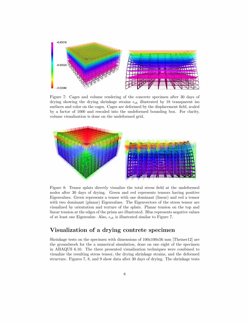
Figure 7: Cages and volume rendering of the concrete specimen after 30 days ofdrying showing the drying shrinkage strains εsh illustrated by 18 transparent isosurfaces and color on the cages. Cages are deformed by the displacement field, scaledby a factor of 1000 and rescaled into the undeformed bounding box. For clarity,volume visualization is done on the undeformed grid.

Figure 8: Tensor splats directly visualize the total stress field at the undeformednodes after 30 days of drying. Green and red represents tensors having positiveEigenvalues. Green represents a tensor with one dominant (linear) and red a tensorwith two dominant (planar) Eigenvalues. The Eigenvectors of the stress tensor arevisualized by orientation and texture of the splats. Planar tension on the top andlinear tension at the edges of the prism are illustrated. Blue represents negative valuesof at least one Eigenvalue. Also, εsh is illustrated similar to Figure 7.

Visualization of a drying contrete specimen

Shrinkage tests on the specimen with dimensions of 100x100x56 mm [Theiner12] arethe groundwork for the a numerical simulation, done on one eight of the specimenin ABAQUS 6.10. The three presented visualization techniques were combined tovisualize the resulting stress tensor, the drying shrinkage strains, and the deformedstructure. Figures 7, 8, and 9 show data after 30 days of drying. The shrinkage tests

8

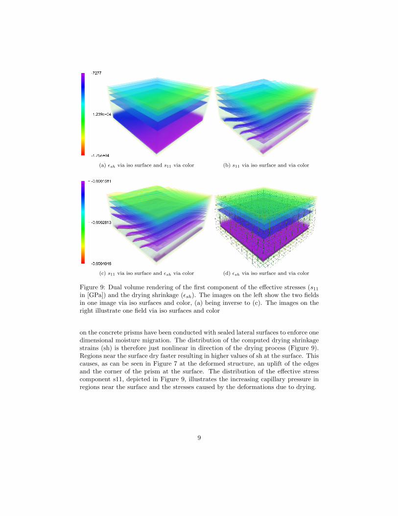
(a) εsh via iso surface and s11 via color (b) s11 via iso surface and via color

(c) s11 via iso surface and εsh via color (d) εsh via iso surface and via color

Figure 9: Dual volume rendering of the first component of the effective stresses (s11in [GPa]) and the drying shrinkage (εsh). The images on the left show the two fieldsin one image via iso surfaces and color, (a) being inverse to (c). The images on theright illustrate one field via iso surfaces and color

on the concrete prisms have been conducted with sealed lateral surfaces to enforce onedimensional moisture migration. The distribution of the computed drying shrinkagestrains (sh) is therefore just nonlinear in direction of the drying process (Figure 9).Regions near the surface dry faster resulting in higher values of sh at the surface. Thiscauses, as can be seen in Figure 7 at the deformed structure, an uplift of the edgesand the corner of the prism at the surface. The distribution of the effective stresscomponent s11, depicted in Figure 9, illustrates the increasing capillary pressure inregions near the surface and the stresses caused by the deformations due to drying.

9

Summary

We presented an approach for advanced visualization of stress and scalar fields givenon a data structure describing finite elements. We propose a highly systematic ap-proach to (re-)organize the data based on the mathematical concepts of fiber bundles.This formulation of interpolation nodes and weights as spatio-temporal data allows toreuse visualization components for displaying scalar fields of our visualization frame-work, hereby being extended for handling FE data. We demonstrated visualizationmethods for displaying displacement and stress field visualization.

References

Benger, W., Hege, H.-C. (2004). “Tensor Splats”, Conference on Visualization and

Data Analysis 2004, Proceedings of SPIE, vol. #5295, p. 151-162.

Benger, W., Ritter, G., and Heinzl, R. (2007). “The Concepts of VISH.”, Proc. 4th High

End Visualization Workshop Obergurgl, Lehmanns Media, p. 26-39.

Benger, W., Haider, M., Stoeckl, J., Biagio, C., Ritter, M., Steinhauser, D., and Hoeller,

H. (2012). “Visualization methods for numerical astrophysics”, Chapter in As-

trophysics, InTechOpenAccess publisher, ISBN 978-953-51-0473-5.

Bock, A., and Sunden, E., Liu, B., Wuensche, B., Ropinski, T. (2012). “Coherency-

Based Curve Compression for High-Order Finite Element Model Visualiza-

tion”, IEEE TVCG (SciVis Proceedings), vol. #18, p. 2315-2324.

Butler, D. M., and Pendley, M. H. (1989). “A visualization model based on the mathe-

matics of fiber bundles”, Comp. in Physics, 3(5), 45-51.

Engel, K., Hadwiger, M., Kniss, J. M., Rezk-Salama, C., and Weiskopf, D. (2006).

“Real-Time Volume Graphics”, AK Peters, ISBN: 1-56881-266-3.

Garrity, M.P. (1990), “Raytracing irregular volume data”. SIGGRAPH Comput. Graph.,

Vol. # 24, p. 35-40, ISSN 0097-8930, ACM, New York, USA.

HDF-Group. (2013). “HDF5 - Home Page”, http://www.hdfgroup.org/HDF5.

Ritter, M. (2009). “Introduction to HDF5 and F5”, CCT Technical Report Series, Lou-

siana State University, CCT-TR-2009-13.

Valentini, B., Theiner, Y., Aschaber, M., Lehar, H., and Hofstetter, G. (2012). “Single-

phase and multi-ph. modeling of concrete struct.”, Eng. Str., ISSN 0141-0296.

Stompel, A., Lum, E.B., Ma, K. (2002). “Visualization of multidimensional, multi-

variate volume data using hardware-accelerated non-photorealistic rendering

techniques”, In Proc. of Pacific Graph. 2002 Conference, IEEE, p. 394-402.

Theiner, Y., and Hofstetter, G. (2012). “Evaluation of the effects of drying shrinkage

on the behavior of concrete structures strengthened by overlays”, Cement and

Concrete Research, vol. 42, i. 9, p. 1286-1297, ISSN 0008-8846.

Williams, P. L. (1992). “Interactive Direct Volume Visualization of Curvilinear and

Unstructured Data”, PHD Thesis, University of Illios.

10