Embed Size (px)
Citation preview
Visual 3D Modeling from Images
Marc PollefeysUniversity of North Carolina – Chapel Hill, USA
Tutorial Notes

ii
Acknowledgments
At this point I would like to thank the people who contributed directly or indirectly to the text for thistutorial. First of all I would like to express my gratitude towards professor Luc Van Gool, head of theIndustrial Image Processing group (VISICS/PSI/ESAT) of the K.U.Leuven. I am very grateful to mycolleagues Maarten Vergauwen and Kurt Cornelis who are not only doing great research work (of whichyou’ll find many examples in this text), but also proofread the whole text. Next I would also like tothank Frank Verbiest, Jan Tops, Joris Schouteden, Reinhard Koch, Tinne Tuytelaars and Benno Heiglwho have contributed to the work presented in this text. I would also like to acknowledge the Fund forScientific Research - Flanders (Belgium) for granting me a Postdoctoral Fellowship. The financial supportof the FWO project G.0223.01 and the European IST projects InViews, Attest, Vibes and Murale are alsogratefully acknowledged.
iii

iv
Notations
To enhance the readability the notations used throughout the text are summarized here.For matrices bold face fonts are used (i.e.
). 4-vectors are represented by and 3-vectors by . Scalar
values will be represented as .Unless stated differently the indices , and are used for views, while and are used for indexing
points, lines or planes. The notation
indicates the entity
which relates view to view (or goingfrom view to view ). The indices , and will also be used to indicate the entries of vectors, matricesand tensors. The subscripts , , and will refer to projective, affine, metric and Euclidean entitiesrespectively
camera projection matrix ( matrix)world point (4-vector)world plane (4-vector) image point (3-vector)image line (3-vector)homography for plane
from view to view ( matrix) homography from plane
to image ( matrix)fundamental matrix ( rank 2 matrix) epipole (projection of projection center of viewpoint into image )trifocal tensor ( tensor)!calibration matrix ( upper triangular matrix)"rotation matrix$#plane at infinity (canonical representation: %'&)( )*absolute conic(canonical representation: +-,/.102,/.435,6&)( and %'&)( )*57absolute dual quadric ( 8 rank 3 matrix)9 # absolute conic embedded in the plane at infinity ( matrix)9 7# dual absolute conic embedded in the plane at infinity ( : matrix)9 image of the absolute conic ( matrices)9 7 dual image of the absolute conic ( matrices); equivalence up to scale ( ;)<>=@?$ACB&D( EF)& AG< )H HJIindicates the Frobenius norm of
(i.e. K L M, )ON P
indicates the matrix
scaled to have unit Frobenius norm(i.e. QR Q R I )TSis the transpose of
VUXW
is the inverse of
(i.e.T UXW & YUZW[ &)\ )T]
is the Moore-Penrose pseudo inverse of
v

vi
Contents
1 Introduction 11.1 3D from images . . . . . . . . . . . . . . . . . . . . . . . . . . . . . . . . . . . . . . . . 21.2 Overview . . . . . . . . . . . . . . . . . . . . . . . . . . . . . . . . . . . . . . . . . . . 3
2 Projective geometry 92.1 Projective geometry . . . . . . . . . . . . . . . . . . . . . . . . . . . . . . . . . . . . . . 9
2.1.1 The projective plane . . . . . . . . . . . . . . . . . . . . . . . . . . . . . . . . . 102.1.2 Projective 3-space . . . . . . . . . . . . . . . . . . . . . . . . . . . . . . . . . . 102.1.3 Transformations . . . . . . . . . . . . . . . . . . . . . . . . . . . . . . . . . . . 102.1.4 Conics and quadrics . . . . . . . . . . . . . . . . . . . . . . . . . . . . . . . . . 11
2.2 The stratification of 3D geometry . . . . . . . . . . . . . . . . . . . . . . . . . . . . . . . 122.2.1 Projective stratum . . . . . . . . . . . . . . . . . . . . . . . . . . . . . . . . . . 132.2.2 Affine stratum . . . . . . . . . . . . . . . . . . . . . . . . . . . . . . . . . . . . 132.2.3 Metric stratum . . . . . . . . . . . . . . . . . . . . . . . . . . . . . . . . . . . . 142.2.4 Euclidean stratum . . . . . . . . . . . . . . . . . . . . . . . . . . . . . . . . . . . 182.2.5 Overview of the different strata . . . . . . . . . . . . . . . . . . . . . . . . . . . 18
2.3 Conclusion . . . . . . . . . . . . . . . . . . . . . . . . . . . . . . . . . . . . . . . . . . 18
3 Camera model and multiple view geometry 213.1 The camera model . . . . . . . . . . . . . . . . . . . . . . . . . . . . . . . . . . . . . . . 21
3.1.1 A simple model . . . . . . . . . . . . . . . . . . . . . . . . . . . . . . . . . . . . 213.1.2 Intrinsic calibration . . . . . . . . . . . . . . . . . . . . . . . . . . . . . . . . . . 213.1.3 Camera motion . . . . . . . . . . . . . . . . . . . . . . . . . . . . . . . . . . . . 233.1.4 The projection matrix . . . . . . . . . . . . . . . . . . . . . . . . . . . . . . . . . 243.1.5 Deviations from the camera model . . . . . . . . . . . . . . . . . . . . . . . . . . 25
3.2 Multi view geometry . . . . . . . . . . . . . . . . . . . . . . . . . . . . . . . . . . . . . 273.2.1 Two view geometry . . . . . . . . . . . . . . . . . . . . . . . . . . . . . . . . . . 273.2.2 Three view geometry . . . . . . . . . . . . . . . . . . . . . . . . . . . . . . . . . 293.2.3 Multi view geometry . . . . . . . . . . . . . . . . . . . . . . . . . . . . . . . . . 31
3.3 Conclusion . . . . . . . . . . . . . . . . . . . . . . . . . . . . . . . . . . . . . . . . . . 31
4 Relating images 334.1 Feature extraction and matching . . . . . . . . . . . . . . . . . . . . . . . . . . . . . . . 33
4.1.1 Comparing image regions . . . . . . . . . . . . . . . . . . . . . . . . . . . . . . 334.1.2 Feature point extraction . . . . . . . . . . . . . . . . . . . . . . . . . . . . . . . 344.1.3 Matching using affinely invariant regions . . . . . . . . . . . . . . . . . . . . . . 36
4.2 Two view geometry computation . . . . . . . . . . . . . . . . . . . . . . . . . . . . . . . 374.2.1 Eight-point algorithm . . . . . . . . . . . . . . . . . . . . . . . . . . . . . . . . . 374.2.2 Seven-point algorithm . . . . . . . . . . . . . . . . . . . . . . . . . . . . . . . . 374.2.3 More points... . . . . . . . . . . . . . . . . . . . . . . . . . . . . . . . . . . . . . 384.2.4 Robust algorithm . . . . . . . . . . . . . . . . . . . . . . . . . . . . . . . . . . . 384.2.5 Degenerate case . . . . . . . . . . . . . . . . . . . . . . . . . . . . . . . . . . . 39
vii
viii CONTENTS
4.3 Three and four view geometry computation . . . . . . . . . . . . . . . . . . . . . . . . . 40
5 Structure and motion 415.1 Initial structure and motion . . . . . . . . . . . . . . . . . . . . . . . . . . . . . . . . . . 41
5.1.1 Initial frame . . . . . . . . . . . . . . . . . . . . . . . . . . . . . . . . . . . . . . 425.1.2 Initializing structure . . . . . . . . . . . . . . . . . . . . . . . . . . . . . . . . . 42
5.2 Updating the structure and motion . . . . . . . . . . . . . . . . . . . . . . . . . . . . . . 425.2.1 projective pose estimation . . . . . . . . . . . . . . . . . . . . . . . . . . . . . . 425.2.2 Relating to other views . . . . . . . . . . . . . . . . . . . . . . . . . . . . . . . . 445.2.3 Refining and extending structure . . . . . . . . . . . . . . . . . . . . . . . . . . . 46
5.3 Refining structure and motion . . . . . . . . . . . . . . . . . . . . . . . . . . . . . . . . 465.4 Dealing with dominant planes . . . . . . . . . . . . . . . . . . . . . . . . . . . . . . . . 48
5.4.1 Detecting dominant planes . . . . . . . . . . . . . . . . . . . . . . . . . . . . . . 485.4.2 Partial projective structure and motion recovery . . . . . . . . . . . . . . . . . . . 505.4.3 Combined metric structure and motion recovery . . . . . . . . . . . . . . . . . . . 50
5.5 Conclusion . . . . . . . . . . . . . . . . . . . . . . . . . . . . . . . . . . . . . . . . . . 52
6 Self-calibration 556.1 Calibration . . . . . . . . . . . . . . . . . . . . . . . . . . . . . . . . . . . . . . . . . . 55
6.1.1 Scene knowledge . . . . . . . . . . . . . . . . . . . . . . . . . . . . . . . . . . . 566.1.2 Camera knowledge . . . . . . . . . . . . . . . . . . . . . . . . . . . . . . . . . . 56
6.2 Self-calibration . . . . . . . . . . . . . . . . . . . . . . . . . . . . . . . . . . . . . . . . 576.2.1 A counting argument . . . . . . . . . . . . . . . . . . . . . . . . . . . . . . . . . 576.2.2 Geometric interpretation of constraints . . . . . . . . . . . . . . . . . . . . . . . 576.2.3 The image of the absolute conic . . . . . . . . . . . . . . . . . . . . . . . . . . . 586.2.4 Self-calibration methods . . . . . . . . . . . . . . . . . . . . . . . . . . . . . . . 596.2.5 Critical motion sequences . . . . . . . . . . . . . . . . . . . . . . . . . . . . . . 60
6.3 A practical approach to self-calibration . . . . . . . . . . . . . . . . . . . . . . . . . . . . 616.3.1 linear self-calibration . . . . . . . . . . . . . . . . . . . . . . . . . . . . . . . . . 626.3.2 non-linear self-calibration refinement . . . . . . . . . . . . . . . . . . . . . . . . 636.3.3 Metric bundle adjustment . . . . . . . . . . . . . . . . . . . . . . . . . . . . . . 63
6.4 Conclusion . . . . . . . . . . . . . . . . . . . . . . . . . . . . . . . . . . . . . . . . . . 64
7 Dense depth estimation 657.1 Image pair rectification . . . . . . . . . . . . . . . . . . . . . . . . . . . . . . . . . . . . 65
7.1.1 Planar rectification . . . . . . . . . . . . . . . . . . . . . . . . . . . . . . . . . . 657.1.2 Polar rectification . . . . . . . . . . . . . . . . . . . . . . . . . . . . . . . . . . . 667.1.3 Examples . . . . . . . . . . . . . . . . . . . . . . . . . . . . . . . . . . . . . . . 69
7.2 Stereo matching . . . . . . . . . . . . . . . . . . . . . . . . . . . . . . . . . . . . . . . . 717.2.1 Exploiting scene constraints . . . . . . . . . . . . . . . . . . . . . . . . . . . . . 717.2.2 Constrained matching . . . . . . . . . . . . . . . . . . . . . . . . . . . . . . . . 73
7.3 Multi-view stereo . . . . . . . . . . . . . . . . . . . . . . . . . . . . . . . . . . . . . . . 767.3.1 Correspondence Linking Algorithm . . . . . . . . . . . . . . . . . . . . . . . . . 767.3.2 Some results . . . . . . . . . . . . . . . . . . . . . . . . . . . . . . . . . . . . . 78
7.4 Conclusion . . . . . . . . . . . . . . . . . . . . . . . . . . . . . . . . . . . . . . . . . . 81
8 Modeling 838.1 Surface model . . . . . . . . . . . . . . . . . . . . . . . . . . . . . . . . . . . . . . . . . 83
8.1.1 Texture enhancement . . . . . . . . . . . . . . . . . . . . . . . . . . . . . . . . . 838.1.2 Volumetric integration . . . . . . . . . . . . . . . . . . . . . . . . . . . . . . . . 85
8.2 Lightfield model . . . . . . . . . . . . . . . . . . . . . . . . . . . . . . . . . . . . . . . . 908.2.1 structure and motion . . . . . . . . . . . . . . . . . . . . . . . . . . . . . . . . . 918.2.2 Lightfield modeling and rendering . . . . . . . . . . . . . . . . . . . . . . . . . . 918.2.3 Experiments . . . . . . . . . . . . . . . . . . . . . . . . . . . . . . . . . . . . . 93
CONTENTS ix
8.2.4 conclusion . . . . . . . . . . . . . . . . . . . . . . . . . . . . . . . . . . . . . . 968.3 Fusion of real and virtual scenes . . . . . . . . . . . . . . . . . . . . . . . . . . . . . . . 96
8.3.1 Augmenting video footage . . . . . . . . . . . . . . . . . . . . . . . . . . . . . . 968.4 Conclusion . . . . . . . . . . . . . . . . . . . . . . . . . . . . . . . . . . . . . . . . . . 97
9 Some results 1019.1 Acquisition of 3D models from photographs . . . . . . . . . . . . . . . . . . . . . . . . . 1019.2 Acquisition of 3D models from pre-existing image sequences . . . . . . . . . . . . . . . . 1079.3 Virtualizing archaeological sites . . . . . . . . . . . . . . . . . . . . . . . . . . . . . . . 108
9.3.1 Virtualizing scenes . . . . . . . . . . . . . . . . . . . . . . . . . . . . . . . . . . 1089.3.2 Reconstructing an overview model . . . . . . . . . . . . . . . . . . . . . . . . . . 1099.3.3 Reconstructions at different scales . . . . . . . . . . . . . . . . . . . . . . . . . . 112
9.4 More applications in archaeology . . . . . . . . . . . . . . . . . . . . . . . . . . . . . . . 1129.4.1 3D stratigraphy . . . . . . . . . . . . . . . . . . . . . . . . . . . . . . . . . . . . 1129.4.2 Generating and testing building hypotheses . . . . . . . . . . . . . . . . . . . . . 113
9.5 Architecture and heritage conservation . . . . . . . . . . . . . . . . . . . . . . . . . . . . 1149.6 Planetary rover control . . . . . . . . . . . . . . . . . . . . . . . . . . . . . . . . . . . . 1159.7 Conclusion . . . . . . . . . . . . . . . . . . . . . . . . . . . . . . . . . . . . . . . . . . 116
A Bundle adjustment 119A.1 Levenberg-Marquardt minimization . . . . . . . . . . . . . . . . . . . . . . . . . . . . . 119
A.1.1 Newton iteration . . . . . . . . . . . . . . . . . . . . . . . . . . . . . . . . . . . 119A.1.2 Levenberg-Marquardt iteration . . . . . . . . . . . . . . . . . . . . . . . . . . . . 120
A.2 Bundle adjustment . . . . . . . . . . . . . . . . . . . . . . . . . . . . . . . . . . . . . . 120

Chapter 1
Introduction
In recent years computer graphics has made tremendous progress in visualizing 3D models. Many tech-niques have reached maturity and are being ported to hardware. This explains that in the area of 3D visual-ization performance is increasing even faster than Moore’s law1. What required a million dollar computera few years ago can now be achieved by a game computer costing a few hundred dollars. It is now possibleto visualize complex 3D scenes in real time.
This evolution causes an important demand for more complex and realistic models. The problem isthat even though the tools that are available for three-dimensional modeling are getting more and morepowerful, synthesizing realistic models is difficult and time-consuming, and thus very expensive. Manyvirtual objects are inspired by real objects and it would therefore be interesting to be able to acquire themodels directly from the real object.
Researchers have been investigating methods to acquire 3D information from objects and scenes formany years. In the past the main applications were visual inspection and robot guidance. Nowadayshowever the emphasis is shifting. There is more and more demand for 3D content for computer graphics,virtual reality and communication. This results in a change in emphasis for the requirements. The visualquality becomes one of the main points of attention. Therefore not only the position of a small number ofpoints have to be measured with high accuracy, but the geometry and appearance of all points of the surfacehave to be measured.
The acquisition conditions and the technical expertise of the users in these new application domainscan often not be matched with the requirements of existing systems. These require intricate calibrationprocedures every time the system is used. There is an important demand for flexibility in acquisition.Calibration procedures should be absent or restricted to a minimum.
Additionally, the existing systems are often built around specialized hardware (e.g. laser range findersor stereo rigs) resulting in a high cost for these systems. Many new applications however require robustlow cost acquisition systems. This stimulates the use of consumer photo- or video cameras. The recentprogress in consumer digital imaging facilitates this. Moore’s law also tells us that more and more can bedone in software.
Due to the convergence of these different factors, many techniques have been developed over the lastfew years. Many of them do not require more than a camera and a computer to acquire three-dimensionalmodels of real objects.
There are active and passive techniques. The former ones control the lighting of the scene (e.g. projec-tion of structured light) which on the one hand simplifies the problem, but on the other hand restricts theapplicability. The latter ones are often more flexible, but computationally more expensive and dependenton the structure of the scene itself.
Some examples of state-of-the-art active techniques are the simple shadow-based approach proposedby Bouguet and Perona [10] or the grid projection approach proposed by Proesmans et al. [126, 133] whichis able to extract dynamic textured 3D shapes (this technique is commercially available, see [133]). Forthe passive techniques many approaches exist. The main differences between the approaches consist of the
1Moore’s law tells us that the density of silicon integrated devices roughly doubles every 18 months.
1
2 CHAPTER 1. INTRODUCTION
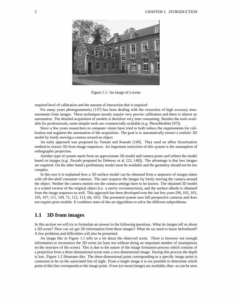
Figure 1.1: An image of a scene
required level of calibration and the amount of interaction that is required.For many years photogrammetry [137] has been dealing with the extraction of high accuracy mea-
surements from images. These techniques mostly require very precise calibration and there is almost noautomation. The detailed acquisition of models is therefore very time consuming. Besides the tools avail-able for professionals, some simpler tools are commercially available (e.g. PhotoModeler [97]).
Since a few years researchers in computer vision have tried to both reduce the requirements for cali-bration and augment the automation of the acquisition. The goal is to automatically extract a realistic 3Dmodel by freely moving a camera around an object.
An early approach was proposed by Tomasi and Kanade [149]. They used an affine factorizationmethod to extract 3D from image sequences. An important restriction of this system is the assumption oforthographic projection.
Another type of system starts from an approximate 3D model and camera poses and refines the modelbased on images (e.g. Facade proposed by Debevec et al. [22, 148]). The advantage is that less imagesare required. On the other hand a preliminary model must be available and the geometry should not be toocomplex.
In this text it is explained how a 3D surface model can be obtained from a sequence of images takenwith off-the-shelf consumer cameras. The user acquires the images by freely moving the camera aroundthe object. Neither the camera motion nor the camera settings have to be known. The obtained 3D modelis a scaled version of the original object (i.e. a metric reconstruction), and the surface albedo is obtainedfrom the image sequence as well. This approach has been developed over the last few years [99, 102, 103,105, 107, 111, 109, 71, 112, 113, 66, 101]. The presented system uses full perspective cameras and doesnot require prior models. It combines state-of-the-art algorithms to solve the different subproblems.
1.1 3D from images
In this section we will try to formulate an answer to the following questions. What do images tell us abouta 3D scene? How can we get 3D information from these images? What do we need to know beforehand?A few problems and difficulties will also be presented.
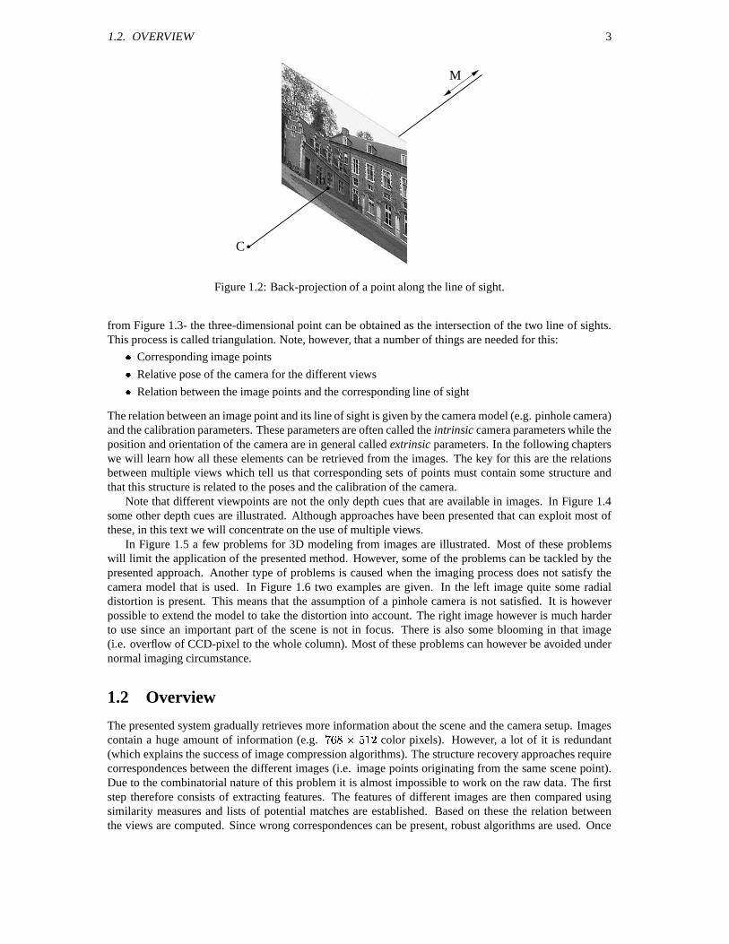
An image like in Figure 1.1 tells us a lot about the observed scene. There is however not enoughinformation to reconstruct the 3D scene (at least not without doing an important number of assumptionson the structure of the scene). This is due to the nature of the image formation process which consists ofa projection from a three-dimensional scene onto a two-dimensional image. During this process the depthis lost. Figure 1.2 illustrates this. The three-dimensional point corresponding to a specific image point isconstraint to be on the associated line of sight. From a single image it is not possible to determine whichpoint of this line corresponds to the image point. If two (or more) images are available, then -as can be seen
1.2. OVERVIEW 3
M
m
C
Figure 1.2: Back-projection of a point along the line of sight.
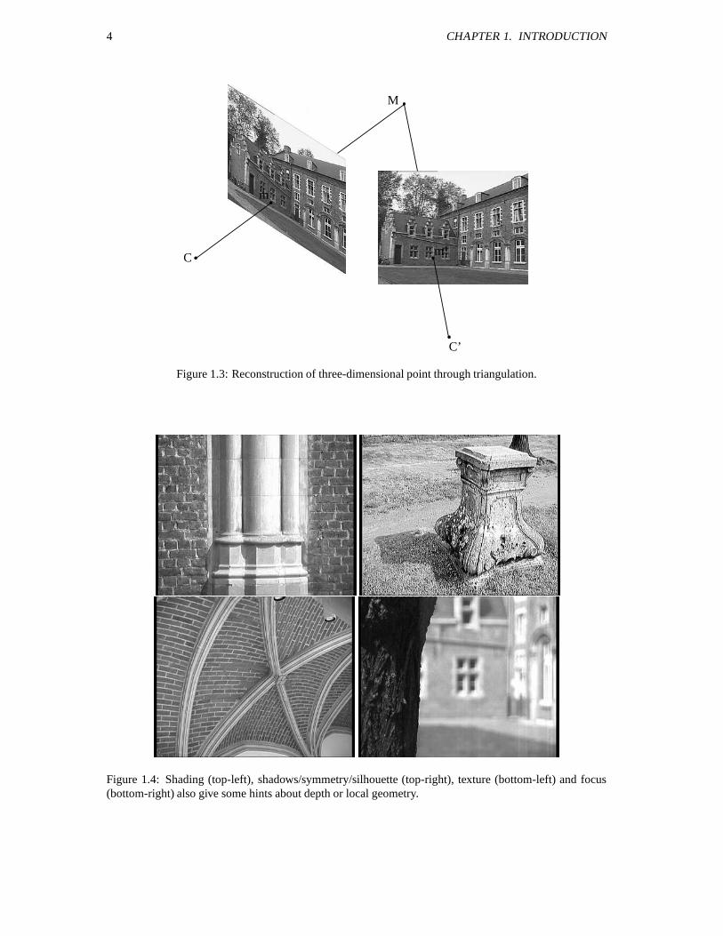
from Figure 1.3- the three-dimensional point can be obtained as the intersection of the two line of sights.This process is called triangulation. Note, however, that a number of things are needed for this:
Corresponding image points Relative pose of the camera for the different views Relation between the image points and the corresponding line of sight
The relation between an image point and its line of sight is given by the camera model (e.g. pinhole camera)and the calibration parameters. These parameters are often called the intrinsic camera parameters while theposition and orientation of the camera are in general called extrinsic parameters. In the following chapterswe will learn how all these elements can be retrieved from the images. The key for this are the relationsbetween multiple views which tell us that corresponding sets of points must contain some structure andthat this structure is related to the poses and the calibration of the camera.
Note that different viewpoints are not the only depth cues that are available in images. In Figure 1.4some other depth cues are illustrated. Although approaches have been presented that can exploit most ofthese, in this text we will concentrate on the use of multiple views.
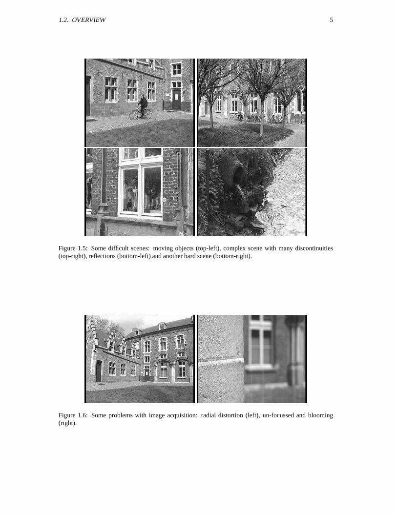
In Figure 1.5 a few problems for 3D modeling from images are illustrated. Most of these problemswill limit the application of the presented method. However, some of the problems can be tackled by thepresented approach. Another type of problems is caused when the imaging process does not satisfy thecamera model that is used. In Figure 1.6 two examples are given. In the left image quite some radialdistortion is present. This means that the assumption of a pinhole camera is not satisfied. It is howeverpossible to extend the model to take the distortion into account. The right image however is much harderto use since an important part of the scene is not in focus. There is also some blooming in that image(i.e. overflow of CCD-pixel to the whole column). Most of these problems can however be avoided undernormal imaging circumstance.
1.2 Overview
The presented system gradually retrieves more information about the scene and the camera setup. Imagescontain a huge amount of information (e.g.
color pixels). However, a lot of it is redundant(which explains the success of image compression algorithms). The structure recovery approaches requirecorrespondences between the different images (i.e. image points originating from the same scene point).Due to the combinatorial nature of this problem it is almost impossible to work on the raw data. The firststep therefore consists of extracting features. The features of different images are then compared usingsimilarity measures and lists of potential matches are established. Based on these the relation betweenthe views are computed. Since wrong correspondences can be present, robust algorithms are used. Once
4 CHAPTER 1. INTRODUCTION
m
M
m’
C’
C
Figure 1.3: Reconstruction of three-dimensional point through triangulation.
Figure 1.4: Shading (top-left), shadows/symmetry/silhouette (top-right), texture (bottom-left) and focus(bottom-right) also give some hints about depth or local geometry.
1.2. OVERVIEW 5
Figure 1.5: Some difficult scenes: moving objects (top-left), complex scene with many discontinuities(top-right), reflections (bottom-left) and another hard scene (bottom-right).
Figure 1.6: Some problems with image acquisition: radial distortion (left), un-focussed and blooming(right).
6 CHAPTER 1. INTRODUCTION
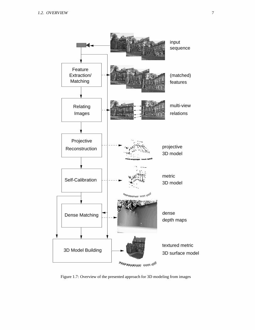
consecutive views have been related to each other, the structure of the features and the motion of thecamera is computed. An initial reconstruction is then made for the first two images of the sequence. Forthe subsequent images the camera pose is estimated in the frame defined by the first two cameras. Forevery additional image that is processed at this stage, the features corresponding to points in previousimages are reconstructed, refined or corrected. Therefore it is not necessary that the initial points stayvisible throughout the entire sequence. The result of this step is a reconstruction of typically a few hundredfeature points. When uncalibrated cameras are used the structure of the scene and the motion of the camerais only determined up to an arbitrary projective transformation. The next step consists of restricting thisambiguity to metric (i.e. Euclidean up to an arbitrary scale factor) through self-calibration. In a projectivereconstruction not only the scene, but also the camera is distorted. Since the algorithm deals with unknownscenes, it has no way of identifying this distortion in the reconstruction. Although the camera is alsoassumed to be unknown, some constraints on the intrinsic camera parameters (e.g. rectangular or squarepixels, constant aspect ratio, principal point in the middle of the image, ...) can often still be assumed.A distortion on the camera mostly results in the violation of one or more of these constraints. A metricreconstruction/calibration is obtained by transforming the projective reconstruction until all the constraintson the cameras intrinsic parameters are satisfied. At this point enough information is available to go backto the images and look for correspondences for all the other image points. This search is facilitated sincethe line of sight corresponding to an image point can be projected to other images, restricting the searchrange to one dimension. By pre-warping the image -this process is called rectification- standard stereomatching algorithms can be used. This step allows to find correspondences for most of the pixels in theimages. From these correspondences the distance from the points to the camera center can be obtainedthrough triangulation. These results are refined and completed by combining the correspondences frommultiple images. Finally all results are integrated in a textured 3D surface reconstruction of the sceneunder consideration. The model is obtained by approximating the depth map with a triangular wire frame.The texture is obtained from the images and mapped onto the surface. An overview of the systems is givenin Figure 1.7.
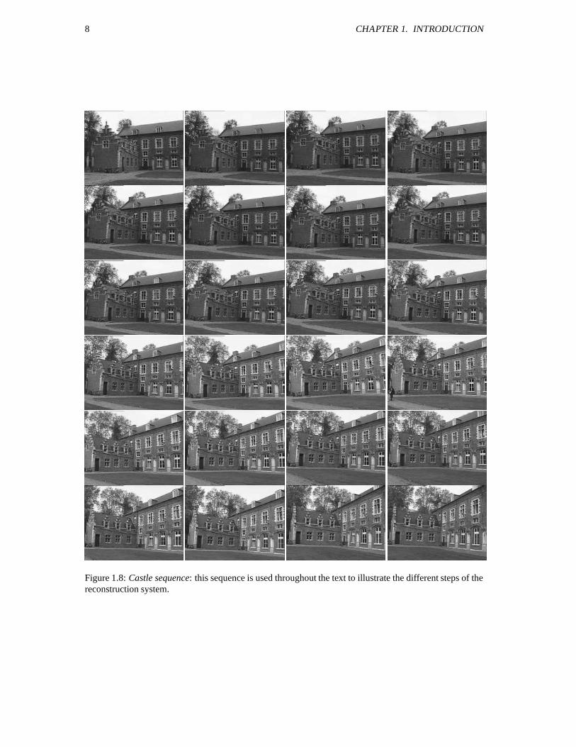
Throughout the rest of the text the different steps of the method will be explained in more detail. Animage sequence of the Arenberg castle in Leuven will be used for illustration. Some of the images of thissequence can be seen in Figure 1.8. The full sequence consists of 24 images recorded with a video camera.
Structure of the notes Chapter 2 and 3 give the geometric foundation to understand the principles behindthe presented approaches. The former introduces projective geometry and the stratification of geometricstructure. The latter describes the perspective camera model and derives the relation between multipleviews. These are at the basis of the possibility to achieve structure and motion recovery. This allows theinterested reader to understand what is behind the techniques presented in the other chapters, but can alsobe skipped.
Chapter 4 deals with the extraction and matching of features and the recovery of multiple view relations.A robust technique is presented to automatically relate two views to each other.
Chapter 5 describes how starting from the relation between consecutive images the structure and motionof the whole sequence can be built up. Chapter 6 briefly describes some self-calibration approaches andproposes a practical method to reduce the ambiguity on the structure and motion to metric.
Chapter 7 is concerned with computing correspondences for all the image points. First an algorithmfor stereo matching is presented. Then rectification is explained. A general method is proposed which cantransform every image pair to standard stereo configuration. Finally, a multi-view approach is presentedwhich allows to obtain denser depth maps and better accuracy.
In Chapter 8 it is explained how the results obtained in the previous chapters can be combined to obtainrealistic models of the acquired scenes. At this point a lot of information is available and different typesof models can be computed. The chapter describes how to obtain surface models and other visual models.The possibility to augment a video sequence is also presented.
1.2. OVERVIEW 7
Matching
Images
3D model
Extraction/ (matched)
projective
Feature
depth maps
sequenceinput
features
Relating
3D surface model
metric
3D model
textured metric
dense
Reconstruction
multi-view
relations
Self-Calibration
3D Model Building
Dense Matching
Projective
Figure 1.7: Overview of the presented approach for 3D modeling from images
8 CHAPTER 1. INTRODUCTION
Figure 1.8: Castle sequence: this sequence is used throughout the text to illustrate the different steps of thereconstruction system.
Chapter 2
Projective geometry
9 A A , M9 A 9 ! " #$" %& ('" 9)%*$ +& "#
“ experience proves that anyone who has studied geometry is infinitely quicker to grasp difficult subjectsthan one who has not.”Plato - The Republic, Book 7, 375 B.C.
The work presented in this text draws a lot on concepts of projective geometry. This chapter and thenext one introduce most of the geometric concepts used in the rest of the text. This chapter concentrateson projective geometry and introduces concepts as points, lines, planes, conics and quadrics in two orthree dimensions. A lot of attention goes to the stratification of geometry in projective, affine, metricand Euclidean layers. Projective geometry is used for its simplicity in formalism, additional structure andproperties can then be introduced were needed through this hierarchy of geometric strata. This sectionwas inspired by the introductions on projective geometry found in Faugeras’ book [29], in the book byMundy and Zisserman (in [91]) and by the book on projective geometry by Semple and Kneebone [132].A detailed account on the subject can be found in the recent book by Hartley and Zisserman [55].
2.1 Projective geometry
A point in projective , -space, -/. , is given by aN ,2.
P-vector of coordinates 0&21 3 W 3 .4 W65
S. At least
one of these coordinates should differ from zero. These coordinates are called homogeneous coordinates.In the text the coordinate vector and the point itself will be indicated with the same symbol. Two pointsrepresented by
N ,V. P-vectors 0 and 7 are equal if and only if there exists a nonzero scalar A such that
3 & A98 , for every N ;: :<,8. P. This will be indicated by 0 ; 7 .
Often the points with coordinate 3 .4 W & ( are said to be at infinity. This is related to the affine space= . . This concept is explained more in detail in section 2.2.A collineation is a mapping between projective spaces, which preserves collinearity (i.e. collinear
points are mapped to collinear points). A collineation from -?> to -@. is mathematically representedby a
N . P N , .
P-matrix
. Points are transformed linearly: 0BACD09E ; 0 . Observe that matrices
and A with A a nonzero scalar represent the same collineation.A projective basis is the extension of a coordinate system to projective geometry. A projective basis is
a set of ,. points such that no ,. of them are linearly dependent. The set %F &G1 ( ( 5 S forevery N H: I:J,.
P, where 1 is in the th position and .4X, &K1 5
Sis the standard projective
basis. A projective point of -/. can be described as a linear combination of any , . points of the standardbasis. For example:
& .4WL
FNM WA F F
It can be shown [31] that any projective basis can be transformed via a uniquely determined collineation
9
10 CHAPTER 2. PROJECTIVE GEOMETRY
into the standard projective basis. Similarly, if two set of points W .4X, and E W E.4X, both forma projective basis, then there exists a uniquely determined collineation
such that EF ; F for every N ;:4(: , . P . This collineation
describes the change of projective basis. In particular,
is invertible.
2.1.1 The projective plane
The projective plane is the projective space -, . A point of -:, is represented by a 3-vector & 1 3 8 5 S .A line
is also represented by a 3-vector. A point is located on a line
if and only if
S & ( (2.1)
This equation can however also be interpreted as expressing that the line
passes through the point . Thissymmetry in the equation shows that there is no formal difference between points and lines in the projectiveplane. This is known as the principle of duality. A line
passing through two points and is given by
their vector product W , . This can also be written as
; 1 W 5 , with 1 W 5 & ( W 8 W W ( 3 W8 W 3 W (
(2.2)
The dual formulation gives the intersection of two lines. All the lines passing through a specific point forma pencil of lines. If two lines
W and, are distinct elements of the pencil, all the other lines can be obtained
through the following equation: ;DA W W . A ,, (2.3)
for some scalars A W and A , . Note that only the ratio is important.
2.1.2 Projective 3-space
Projective 3D space is the projective space - . A point of - is represented by a 4-vector & 1 + 043V% 5 S .
In - the dual entity of a point is a plane, which is also represented by a 4-vector. A point
is located ona plane
if and only if S & ( (2.4)
A line can be given by the linear combination of two points A W W . A ,, or by the intersection of two
planes W , .
2.1.3 Transformations
Transformations in the images are represented by homographies of - , C - , . A homography of - , C - ,is represented by a -matrix
. Again
and A represent the same homography for all nonzero scalarsA . A point is transformed as follows: AC E ; (2.5)
The corresponding transformation of a line can be obtained by transforming the points which are on theline and then finding the line defined by these points:
E S E & S UXW & S &)( (2.6)
From the previous equation the transformation equation for a line is easily obtained (with UZS & N UXWJP S &N S/P UZW
): AC E ; U S (2.7)
Similar reasoning in - gives the following equations for transformations of points and planes in 3D space: AC E ; (2.8) AC E ; U S (2.9)
where
is a 8 -matrix.
2.1. PROJECTIVE GEOMETRY 11
2.1.4 Conics and quadrics
Conic A conic in -2, is the locus of all points satisfying a homogeneous quadratic equation: N P & S &D( (2.10)
where
is a V symmetric matrix only defined up to scale. A conic thus depends on five independentparameters.
Dual conic Similarly, the dual concept exists for lines. A conic envelope or dual conic is the locus of alllines
satisfying a homogeneous quadratic equation:
S 7 &)( (2.11)
where 7
is a T- symmetric matrix only defined up to scale. A dual conic thus also depends on fiveindependent parameters.
Line-conic intersection Let and E be two points defining a line. A point on this line can then berepresented by . A E . This point lies on a conic
if and only if
N . A E P &)( which can also be written as
N P . A N E P . A , N E P & ( (2.12)
where N E P & S E & N E P
This means that a line has in general two intersection points with a conic. These intersection points can bereal or complex and can be obtained by solving equation (2.12).
Tangent to a conic The two intersection points of a line with a conic coincide if the discriminant ofequation (2.12) is zero. This can be written as
N E P N P N E P &)( If the point is considered fixed, this forms a quadratic equation in the coordinates of E which representsthe two tangents from to the conic. If belongs to the conic,
N P & ( and the equation of the tangentsbecomes
N E P & S E &D( which is linear in the coefficients of E . This means that there is only one tangent to the conic at a point ofthe conic. This tangent
is thus represented by : ; S & (2.13)
Relation between conic and dual conic When varies along the conic, it satisfies S and thus thetangent line
to the conic at satisfies
S UZW & ( . This shows that the tangents to a conic
arebelonging to a dual conic
7 ; UXW(assuming
is of full rank).
Transformation of a conic/dual conic The transformation equations for conics and dual conics undera homography
can be obtained in a similar way to Section 2.1.3. Using equations (2.5) and (2.7) the
following is obtained: E S E E ; S S UZS UXW &)( E S 7 E E ; S UZW 7 S UZS &D(
and thus AC E ; U S UXW (2.14) 7 AC 7 E ; 7 S (2.15)
Observe that (2.14) and (2.15) also imply thatN E P 7 & N 7 P E .
12 CHAPTER 2. PROJECTIVE GEOMETRY
Quadric In projective 3-space - similar concepts exist. These are quadrics. A quadric is the locus ofall points
satisfying a homogeneous quadratic equation:
S &D( (2.16)
where
is a symmetric matrix only defined up to scale. A quadric thus depends on nine independentparameters.
Dual quadric Similarly, the dual concept exists for planes. A dual quadric is the locus of all planes
satisfying a homogeneous quadratic equation:
S 7 &)( (2.17)
where 7
is a T symmetric matrix only defined up to scale and thus also depends on nine independentparameters.
Tangent to a quadric Similar to equation (2.13), the tangent plane
to a quadric
through a point
ofthe quadric is obtained as & (2.18)
Relation between quadric and dual quadric When
varies along the quadric, it satisfies S
andthus the tangent plane
to
at
satisfies S UXW &>( . This shows that the tangent planes to a quadric
are belonging to a dual quadric
7 ; UXW (assuming
is of full rank).
Transformation of a quadric/dual quadric The transformation equations for quadrics and dual quadricsunder a homography
can be obtained in a similar way to Section 2.1.3. Using equations (2.8) and (2.9)
the following is obtained
E S E E ; S S U S UZW &)( E S 7 E E ; S UXW 7 S U S &)(and thus
AC E ; U S UXW (2.19) 7 AC 7 E ; 7 S (2.20)
Observe again thatN E P 7 & N 7 P E .
2.2 The stratification of 3D geometry
Usually the world is perceived as a Euclidean 3D space. In some cases (e.g. starting from images) it is notpossible or desirable to use the full Euclidean structure of 3D space. It can be interesting to only deal withthe less structured and thus simpler projective geometry. Intermediate layers are formed by the affine andmetric geometry. These structures can be thought of as different geometric strata which can be overlaid onthe world. The simplest being projective, then affine, next metric and finally Euclidean structure.
This concept of stratification is closely related to the groups of transformations acting on geometricentities and leaving invariant some properties of configurations of these elements. Attached to the projectivestratum is the group of projective transformations, attached to the affine stratum is the group of affinetransformations, attached to the metric stratum is the group of similarities and attached to the Euclideanstratum is the group of Euclidean transformations. It is important to notice that these groups are subgroupsof each other, e.g. the metric group is a subgroup of the affine group and both are subgroups of the projectivegroup.
An important aspect related to these groups are their invariants. An invariant is a property of a con-figuration of geometric entities that is not altered by any transformation belonging to a specific group.
2.2. THE STRATIFICATION OF 3D GEOMETRY 13
Invariants therefore correspond to the measurements that one can do considering a specific stratum of ge-ometry. These invariants are often related to geometric entities which stay unchanged – at least as a whole– under the transformations of a specific group. These entities play an important role in part of this text.Recovering them allows to upgrade the structure of the geometry to a higher level of the stratification.
In the following paragraphs the different strata of geometry are discussed. The associated groups oftransformations, their invariants and the corresponding invariant structures are presented. This idea ofstratification can be found back in [132] and [30].
2.2.1 Projective stratum
The first stratum is the projective one. It is the less structured one and has therefore the least number of in-variants and the largest group of transformations associated with it. The group of projective transformationsor collineations is the most general group of linear transformations.
As seen in the previous chapter a projective transformation of 3D space can be represented by a invertible matrix
; W W W , W W , W , , , , W , JW ,
(2.21)
This transformation matrix is only defined up to a nonzero scale factor and has therefore 15 degrees offreedom.
Relations of incidence, collinearity and tangency are projectively invariant. The cross-ratio is an invari-ant property under projective transformations as well. It is defined as follows: Assume that the four points W , and
are collinear. Then they can be expressed as & . A E (assume none is coincident
with E ). The cross-ratio is defined as
W , & A W A A W A E A , A A , A (2.22)
The cross-ratio is not depending on the choice of the reference points
and E and is invariant under the
group of projective transformations of - . A similar cross-ratio invariant can be derived for four linesintersecting in a point or four planes intersecting in a common line.
The cross-ratio can in fact be seen as the coordinate of a fourth point in the basis of the first three, sincethree points form a basis for the projective line - W . Similarly, two invariants could be obtained for fivecoplanar points; and, three invariants for six points, all in general position.
2.2.2 Affine stratum
The next stratum is the affine one. In the hierarchy of groups it is located in between the projective and themetric group. This stratum contains more structure than the projective one, but less than the metric or theEuclidean strata. Affine geometry differs from projective geometry by identifying a special plane, calledthe plane at infinity.
This plane is usually defined by %'&)( and thus # & 1 ( ( ( 5 S . The projective space can be seen as
containing the affine space under the mapping= C - E1 + 013 5 S AC 1 + 013 5 S . This is a one-to-one
mapping. The plane % & ( in - can be seen as containing the limit points forH H C , since these
points are 1R RR RR R WR R 5 S ; 1 + # 0 # 3 # ( 5 . This plane is therefore called the plane at infinity #
.Strictly speaking, this plane is not part of the affine space, the points contained in it can’t be expressedthrough the usual non-homogeneous 3-vector coordinate notation used for affine, metric and Euclidean 3Dspace.
An affine transformation is usually presented as follows: + E0@E3 E
&
W W W , W , W , , , W , +
03
.
W ,
with N P B& (
14 CHAPTER 2. PROJECTIVE GEOMETRY
Using homogeneous coordinates, this can be rewritten as follows E ; with
; W W W , W W , W , , , , W , ( ( (
(2.23)
An affine transformation counts 12 independent degrees of freedom. It can easily be verified that thistransformation leaves the plane at infinity
G#unchanged (i.e.
G# ; UZS $#or S # ; # ). Note,
however, that the position of points in the plane at infinity can change under an affine transformation, butthat all these points stay within the plane
#.
All projective properties are a fortiori affine properties. For the (more restrictive) affine group paral-lelism is added as a new invariant property. Lines or planes having their intersection in the plane at infinityare called parallel. A new invariant property for this group is the ratio of lengths along a certain direction.Note that this is equivalent to a cross-ratio with one of the points at infinity.
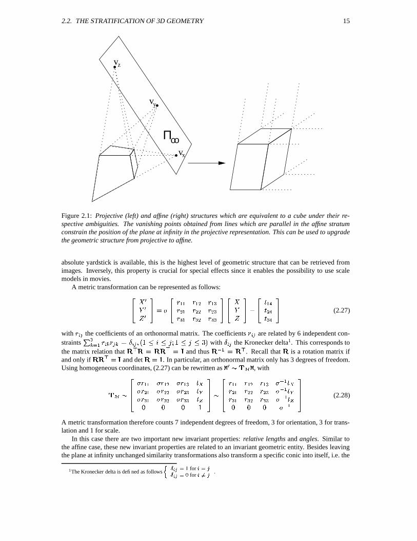
From projective to affine Up to now it was assumed that these different strata could simply be overlaidonto each other, assuming that the plane at infinity is at its canonical position (i.e.
# & 1 ( (/( 5 S ). Thisis easy to achieve when starting from a Euclidean representation. Starting from a projective representation,however, the structure is only determined up to an arbitrary projective transformation. As was seen, thesetransformations do – in general – not leave the plane at infinity unchanged.
Therefore, in a specific projective representation, the plane at infinity can be anywhere. In this caseupgrading the geometric structure from projective to affine implies that one first has to find the position ofthe plane at infinity in the particular projective representation under consideration.
This can be done when some affine properties of the scene are known. Since parallel lines or planesare intersecting in the plane at infinity, this gives constraints on the position of this plane. In Figure 2.1 aprojective representation of a cube is given. Knowing this is a cube, three vanishing points can be identified.The plane at infinity is the plane containing these 3 vanishing points.
Ratios of lengths along a line define the point at infinity of that line. In this case the points
, W , ,
and the cross-ratio W , $# are known, therefore the point
G#can be computed.
Once the plane at infinityG#
is known, one can upgrade the projective representation to an affine oneby applying a transformation which brings the plane at infinity to its canonical position. Based on (2.9)this equation should therefore satisfy
(((
; U S $# or
S (((
; $# (2.24)
This determines the fourth row of
. Since, at this level, the other elements are not constrained, the obviouschoice for the transformation is the following
; \ ( S# (2.25)
with # the first 3 elements of #
when the last element is scaled to 1. It is important to note, however,that every transformation of the form ( S# with B& ( (2.26)
maps$#
to 1 ( ( ( 5 S .
2.2.3 Metric stratum
The metric stratum corresponds to the group of similarities. These transformations correspond to Euclideantransformations (i.e. orthonormal transformation + translation) complemented with a scaling. When no
2.2. THE STRATIFICATION OF 3D GEOMETRY 15
v
v
v
Π οοx
z
y
Figure 2.1: Projective (left) and affine (right) structures which are equivalent to a cube under their re-spective ambiguities. The vanishing points obtained from lines which are parallel in the affine stratumconstrain the position of the plane at infinity in the projective representation. This can be used to upgradethe geometric structure from projective to affine.
absolute yardstick is available, this is the highest level of geometric structure that can be retrieved fromimages. Inversely, this property is crucial for special effects since it enables the possibility to use scalemodels in movies.
A metric transformation can be represented as follows: + E0@E3 E
&
W W W , W
, W, ,
, W ,
+03
.
W,
(2.27)
with
the coefficients of an orthonormal matrix. The coefficients
are related by 6 independent con-straints K M W & N :> :) :D :> P with L the Kronecker delta1. This corresponds tothe matrix relation that
" S " & "T" S & \ and thus" UXW & " S . Recall that
"is a rotation matrix if
and only if" " S &D\ and det
" & . In particular, an orthonormal matrix only has 3 degrees of freedom.Using homogeneous coordinates, (2.27) can be rewritten as
E ; , with
; W W W , W
, W , , , W , ( ( (
;
W W W ,
W UZW
, W, ,
, UXW W , UZW ( ( ( UZW
(2.28)
A metric transformation therefore counts 7 independent degrees of freedom, 3 for orientation, 3 for trans-lation and 1 for scale.
In this case there are two important new invariant properties: relative lengths and angles. Similar tothe affine case, these new invariant properties are related to an invariant geometric entity. Besides leavingthe plane at infinity unchanged similarity transformations also transform a specific conic into itself, i.e. the
1The Kronecker delta is defined as follows
for for .
16 CHAPTER 2. PROJECTIVE GEOMETRY
ΩΠ oo
*
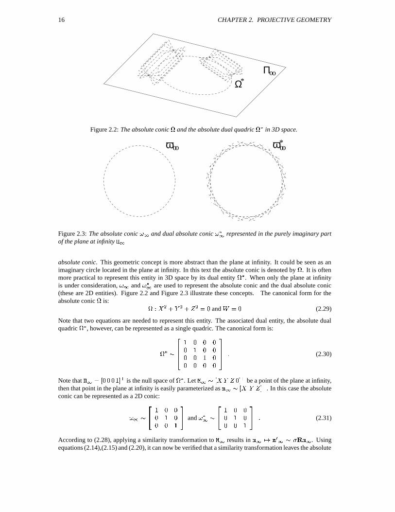
Figure 2.2: The absolute conic*
and the absolute dual quadric* 7
in 3D space.
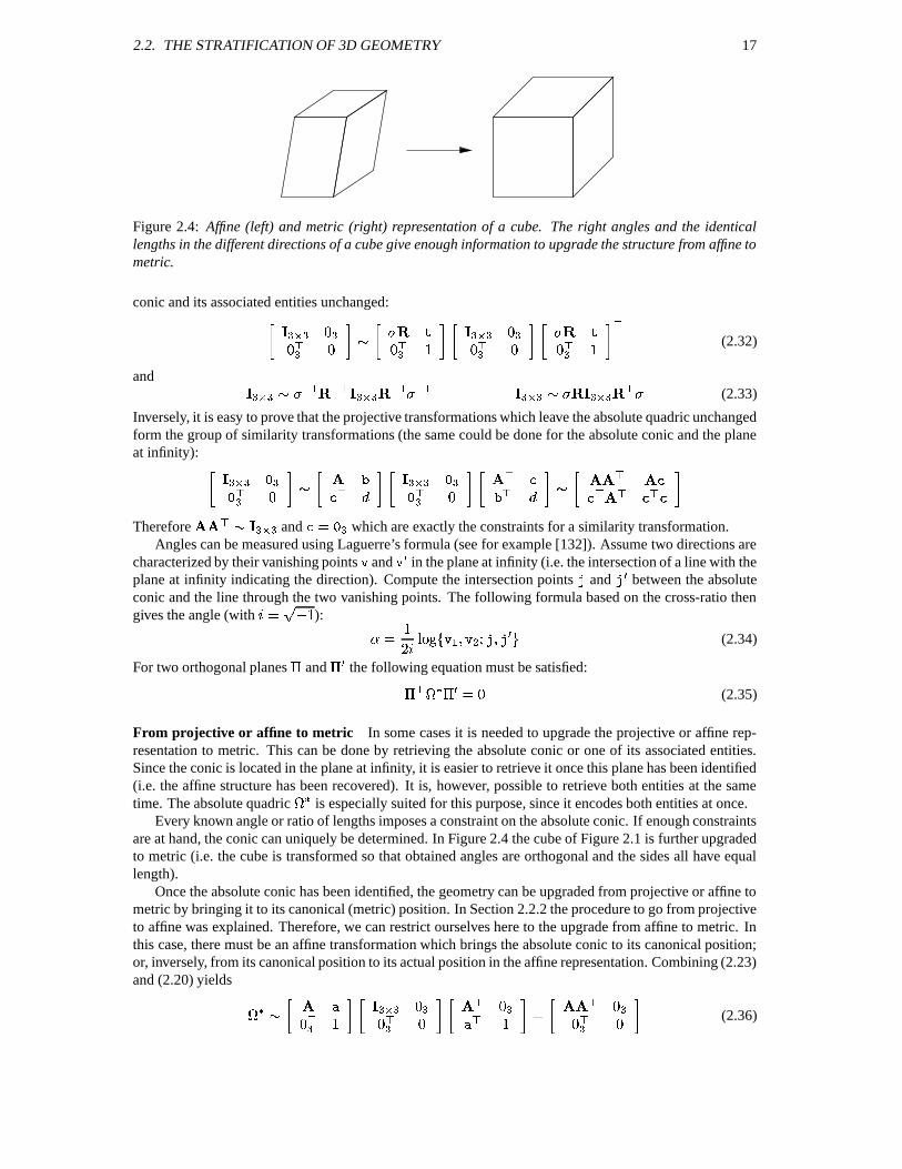
*ωω oooo
Figure 2.3: The absolute conic 9 # and dual absolute conic 9 7# represented in the purely imaginary partof the plane at infinity
G#
absolute conic. This geometric concept is more abstract than the plane at infinity. It could be seen as animaginary circle located in the plane at infinity. In this text the absolute conic is denoted by
*. It is often
more practical to represent this entity in 3D space by its dual entity* 7
. When only the plane at infinityis under consideration, 9 # and 9 7# are used to represent the absolute conic and the dual absolute conic(these are 2D entities). Figure 2.2 and Figure 2.3 illustrate these concepts. The canonical form for theabsolute conic
*is: * EF+ , .10 , .43 , &)( and %'&D( (2.29)
Note that two equations are needed to represent this entity. The associated dual entity, the absolute dualquadric
*57, however, can be represented as a single quadric. The canonical form is:
* 7 ; ( ( (( ( (( ( (( ( ( (
(2.30)
Note that$# &21 ( ( ( 5 S is the null space of
*57. Let
$# ; 1 +>013V( 5 S be a point of the plane at infinity,then that point in the plane at infinity is easily parameterized as # ; 1 + 013 5 S . In this case the absoluteconic can be represented as a 2D conic:
9 # ; ( (( (( (
and 9 7# ;
( (( (( (
(2.31)
According to (2.28), applying a similarity transformation to #
results in # AC E # ; " # . Usingequations (2.14),(2.15) and (2.20), it can now be verified that a similarity transformation leaves the absolute
2.2. THE STRATIFICATION OF 3D GEOMETRY 17
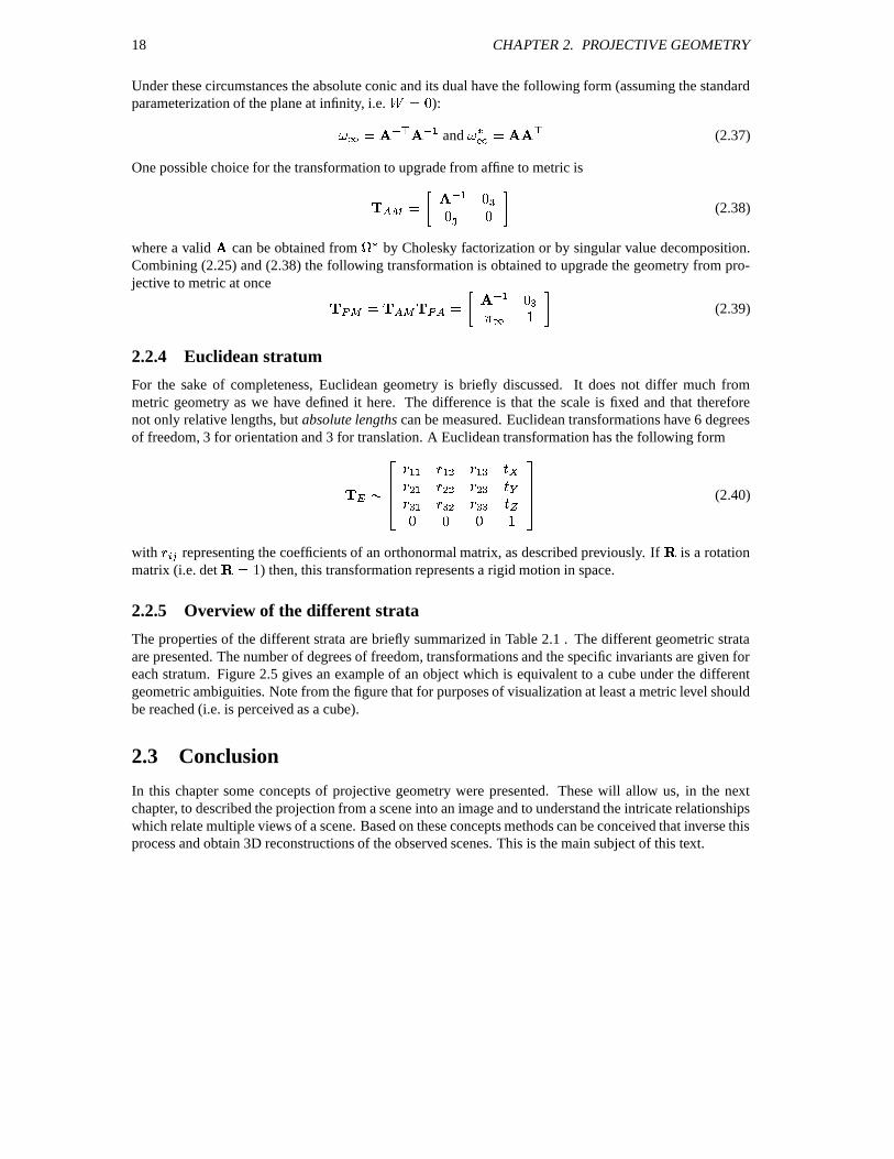
Figure 2.4: Affine (left) and metric (right) representation of a cube. The right angles and the identicallengths in the different directions of a cube give enough information to upgrade the structure from affine tometric.
conic and its associated entities unchanged: \ ( ( S ( ; " ( S \ ( ( S ( "
( S S (2.32)
and\ ; UZW " U S \ " UZW UXW \ ; " \ " S (2.33)
Inversely, it is easy to prove that the projective transformations which leave the absolute quadric unchangedform the group of similarity transformations (the same could be done for the absolute conic and the planeat infinity): \ S ( ;
S \ S ( TS GS ; S S TS S
ThereforeTTS ; \ and & which are exactly the constraints for a similarity transformation.
Angles can be measured using Laguerre’s formula (see for example [132]). Assume two directions arecharacterized by their vanishing points and 9E in the plane at infinity (i.e. the intersection of a line with theplane at infinity indicating the direction). Compute the intersection points and 9E between the absoluteconic and the line through the two vanishing points. The following formula based on the cross-ratio thengives the angle (with & ):
& W , E (2.34)
For two orthogonal planes and E the following equation must be satisfied:
S * 7 E &)( (2.35)
From projective or affine to metric In some cases it is needed to upgrade the projective or affine rep-resentation to metric. This can be done by retrieving the absolute conic or one of its associated entities.Since the conic is located in the plane at infinity, it is easier to retrieve it once this plane has been identified(i.e. the affine structure has been recovered). It is, however, possible to retrieve both entities at the sametime. The absolute quadric
* 7is especially suited for this purpose, since it encodes both entities at once.
Every known angle or ratio of lengths imposes a constraint on the absolute conic. If enough constraintsare at hand, the conic can uniquely be determined. In Figure 2.4 the cube of Figure 2.1 is further upgradedto metric (i.e. the cube is transformed so that obtained angles are orthogonal and the sides all have equallength).
Once the absolute conic has been identified, the geometry can be upgraded from projective or affine tometric by bringing it to its canonical (metric) position. In Section 2.2.2 the procedure to go from projectiveto affine was explained. Therefore, we can restrict ourselves here to the upgrade from affine to metric. Inthis case, there must be an affine transformation which brings the absolute conic to its canonical position;or, inversely, from its canonical position to its actual position in the affine representation. Combining (2.23)and (2.20) yields
* 7 ; ( S \ ( ( S ( S ( S & TS ( ( S ( (2.36)
18 CHAPTER 2. PROJECTIVE GEOMETRY
Under these circumstances the absolute conic and its dual have the following form (assuming the standardparameterization of the plane at infinity, i.e. % &)( ):
9 # & U S UZW and 9 7# & T S (2.37)
One possible choice for the transformation to upgrade from affine to metric is
& UZW ( ( S ( (2.38)
where a valid
can be obtained from* 7
by Cholesky factorization or by singular value decomposition.Combining (2.25) and (2.38) the following transformation is obtained to upgrade the geometry from pro-jective to metric at once & & VUZW ( # (2.39)
2.2.4 Euclidean stratum
For the sake of completeness, Euclidean geometry is briefly discussed. It does not differ much frommetric geometry as we have defined it here. The difference is that the scale is fixed and that thereforenot only relative lengths, but absolute lengths can be measured. Euclidean transformations have 6 degreesof freedom, 3 for orientation and 3 for translation. A Euclidean transformation has the following form
; W W W ,
W
, W, ,
,
W , ( ( (
(2.40)
with L
representing the coefficients of an orthonormal matrix, as described previously. If"
is a rotationmatrix (i.e. det
" & ) then, this transformation represents a rigid motion in space.
2.2.5 Overview of the different strata
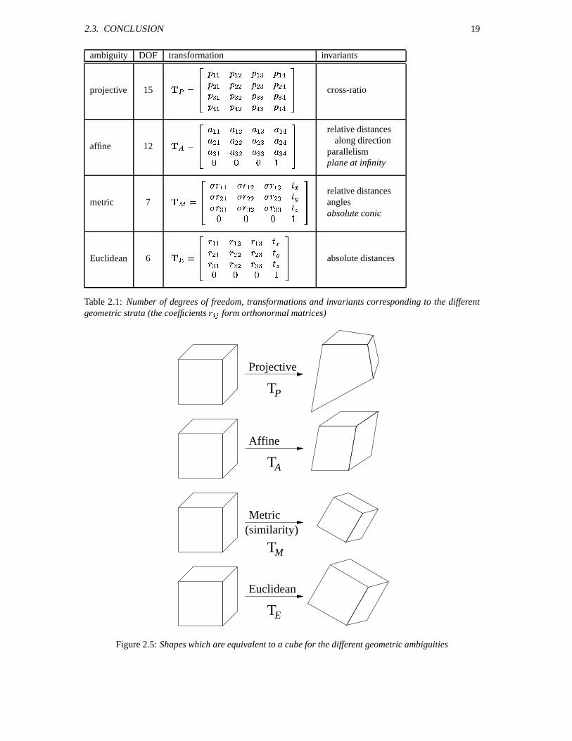
The properties of the different strata are briefly summarized in Table 2.1 . The different geometric strataare presented. The number of degrees of freedom, transformations and the specific invariants are given foreach stratum. Figure 2.5 gives an example of an object which is equivalent to a cube under the differentgeometric ambiguities. Note from the figure that for purposes of visualization at least a metric level shouldbe reached (i.e. is perceived as a cube).
2.3 Conclusion
In this chapter some concepts of projective geometry were presented. These will allow us, in the nextchapter, to described the projection from a scene into an image and to understand the intricate relationshipswhich relate multiple views of a scene. Based on these concepts methods can be conceived that inverse thisprocess and obtain 3D reconstructions of the observed scenes. This is the main subject of this text.
2.3. CONCLUSION 19
ambiguity DOF transformation invariants
projective 15 &
W W W , W W , W , , , , W , [W ,
cross-ratio
affine 12 &
W W W , W W , W , , , , W , ( ( (
relative distances
along directionparallelismplane at infinity
metric 7 &
W W W , W
, W , , , W ,
( ( (
relative distances
anglesabsolute conic
Euclidean 6 &
W W W ,
W
, W, ,
,
W ,
( ( (
absolute distances
Table 2.1: Number of degrees of freedom, transformations and invariants corresponding to the differentgeometric strata (the coefficients
Lform orthonormal matrices)
Metric(similarity)
Projective
Euclidean
Affine
T
A
E
M
T
T
T
P
Figure 2.5: Shapes which are equivalent to a cube for the different geometric ambiguities

20 CHAPTER 2. PROJECTIVE GEOMETRY
Chapter 3
Camera model and multiple viewgeometry
Before discussing how 3D information can be obtained from images it is important to know how imagesare formed. First, the camera model is introduced; and then some important relationships between multipleviews of a scene are presented.
3.1 The camera model
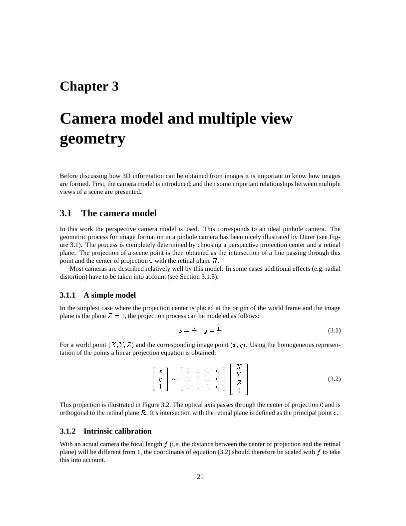
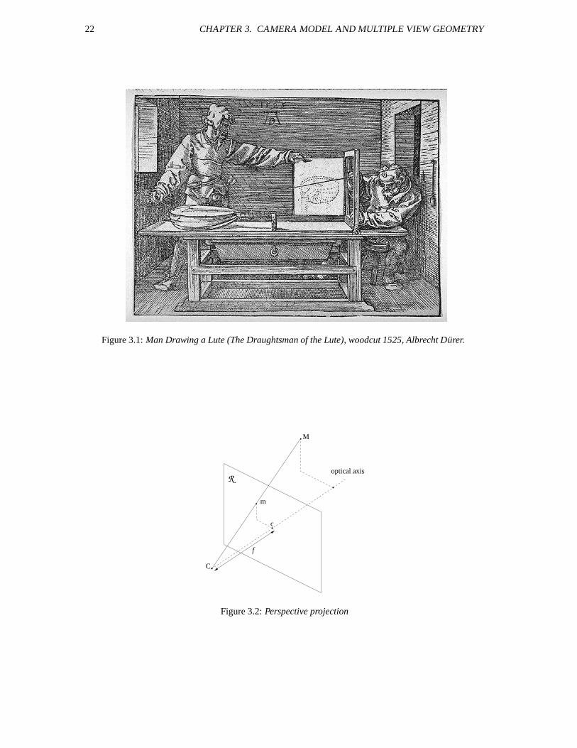
In this work the perspective camera model is used. This corresponds to an ideal pinhole camera. Thegeometric process for image formation in a pinhole camera has been nicely illustrated by Durer (see Fig-ure 3.1). The process is completely determined by choosing a perspective projection center and a retinalplane. The projection of a scene point is then obtained as the intersection of a line passing through thispoint and the center of projection
with the retinal plane .
Most cameras are described relatively well by this model. In some cases additional effects (e.g. radialdistortion) have to be taken into account (see Section 3.1.5).
3.1.1 A simple model
In the simplest case where the projection center is placed at the origin of the world frame and the imageplane is the plane 3D& , the projection process can be modeled as follows:
3T& 8 & (3.1)
For a world pointN + 0 3 P and the corresponding image point
N 3 8 P . Using the homogeneous represen-tation of the points a linear projection equation is obtained:
3 8
;
( ( (( ( (( ( (
+ 03
(3.2)
This projection is illustrated in Figure 3.2. The optical axis passes through the center of projection
and isorthogonal to the retinal plane . It’s intersection with the retinal plane is defined as the principal point .
3.1.2 Intrinsic calibration
With an actual camera the focal length (i.e. the distance between the center of projection and the retinalplane) will be different from 1, the coordinates of equation (3.2) should therefore be scaled with to takethis into account.
21
22 CHAPTER 3. CAMERA MODEL AND MULTIPLE VIEW GEOMETRY
Figure 3.1: Man Drawing a Lute (The Draughtsman of the Lute), woodcut 1525, Albrecht Durer.
m
C
M
optical axis
f
R
c
Figure 3.2: Perspective projection
3.1. THE CAMERA MODEL 23
py
xe
Rp
ye
x
c
Kp
px
α
pixely
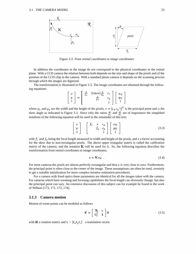
Figure 3.3: From retinal coordinates to image coordinates
In addition the coordinates in the image do not correspond to the physical coordinates in the retinalplane. With a CCD camera the relation between both depends on the size and shape of the pixels and of theposition of the CCD chip in the camera. With a standard photo camera it depends on the scanning processthrough which the images are digitized.
The transformation is illustrated in Figure 3.3. The image coordinates are obtained through the follow-ing equations: 3 8
&
N P
3 8
where and are the width and the height of the pixels, & 1 5 S is the principal point and theskew angle as indicated in Figure 3.3. Since only the ratios and are of importance the simplifiednotations of the following equation will be used in the remainder of this text: 3 8
&
3 8
(3.3)
with and being the focal length measured in width and height of the pixels, and a factor accountingfor the skew due to non-rectangular pixels. The above upper triangular matrix is called the calibrationmatrix of the camera; and the notation
!will be used for it. So, the following equation describes the
transformation from retinal coordinates to image coordinates.
& ! (3.4)
For most cameras the pixels are almost perfectly rectangular and thus is very close to zero. Furthermore,the principal point is often close to the center of the image. These assumptions can often be used, certainlyto get a suitable initialization for more complex iterative estimation procedures.
For a camera with fixed optics these parameters are identical for all the images taken with the camera.For cameras which have zooming and focusing capabilities the focal length can obviously change, but alsothe principal point can vary. An extensive discussion of this subject can for example be found in the workof Willson [173, 171, 172, 174].
3.1.3 Camera motion
Motion of scene points can be modeled as follows
E & " ( S (3.5)
with"
a rotation matrix and & 1
5 S a translation vector.
24 CHAPTER 3. CAMERA MODEL AND MULTIPLE VIEW GEOMETRY
The motion of the camera is equivalent to an inverse motion of the scene and can therefore be modeledas E &
" S " S ( S (3.6)
with"
and
indicating the motion of the camera.
3.1.4 The projection matrix
Combining equations (3.2), (3.3) and (3.6) the following expression is obtained for a camera with somespecific intrinsic calibration and with a specific position and orientation:
3 8
;
(
( (
( ( (( ( (( ( (
" S-" S
( S + 03
which can be simplified to ; ! 1 " S -" S 5 (3.7)
or even ; (3.8)
The T matrix
is called the camera projection matrix.Using (3.8) the plane corresponding to a back-projected image line
can also be obtained: Since S ; S ; S , ; S (3.9)
The transformation equation for projection matrices can be obtained as described in paragraph 2.1.3. If thepoints of a calibration grid are transformed by the same transformation as the camera, their image pointsshould stay the same: ; E E ; UZW ; (3.10)
and thus AC E ; UZW (3.11)
The projection of the outline of a quadric can also be obtained. For a line in an image to be tangent to theprojection of the outline of a quadric, the corresponding plane should be on the dual quadric. Substitutingequation (3.9) in (2.17) the following constraint
S 7 S & ( is obtained for
to be tangent to theoutline. Comparing this result with the definition of a conic (2.10), the following projection equation isobtained for quadrics (this results can also be found in [65]). :
7 ; 7 S (3.12)
Relation between projection matrices and image homographies
The homographies that will be discussed here are collineations from - , C -2, . A homography
de-scribes the transformation from one plane to another. A number of special cases are of interest, since theimage is also a plane. The projection of points of a plane into an image can be described through a ho-mography
. The matrix representation of this homography is dependent on the choice of the projectivebasis in the plane.
As an image is obtained by perspective projection, the relation between points belonging to a plane
in 3D space and their projections in the image is mathematically expressed by a homography .
The matrix of this homography is found as follows. If the plane
is given by ; 1 S 5 S and the point
of
is represented as ; 1 S 5 S , then
belongs to
if and only if (2& S & S . . Hence,
; & S & \ S (3.13)
3.1. THE CAMERA MODEL 25
Now, if the camera projection matrix is &21 5 , then the projection of
onto the image is
; & 1 5 \ S
& 1 S 5 (3.14)
Consequently, ; T S .
Note that for the specific plane & 1 ( (/( 5 S the homographies are simply given by
; T .It is also possible to define homographies which describe the transfer from one image to the other for
points and other geometric entities located on a specific plane. The notation
will be used to describesuch a homography from view to for a plane
. These homographies can be obtained through the
following relation & UXW and are independent to reparameterizations of the plane (and thus also
to a change of basis in - ).In the metric and Euclidean case,
& ! " S and the plane at infinity isG# &21 (F( ( 5 S . In this case,
the homographies for the plane at infinity can thus be written as: # & ! " S ! UXW (3.15)
where" L & " S " is the rotation matrix that describes the relative orientation from the camera with
respect top the one.In the projective and affine case, one can assume that
W & 1 \ 5 (since in this case!
is un-known). In that case, the homographies
W ; \ for all planes; and thus, W &
. Therefore
can be factorized as &21 W W 5 (3.16)
where W is the projection of the center of projection of the first camera (in this case, 1 (/( ( 5 S ) in image . This point W is called the epipole, for reasons which will become clear in Section 3.2.1.
Note that this equation can be used to obtain W and W from
, but that due to the unknown relative
scale factors
can, in general, not be obtained from W and W . Observe also that, in the affine case
(where # &21 (F( ( 5 S ), this yields
&21 # W W 5 .
Combining equations (3.14) and (3.16), one obtains W &
W W S (3.17)
This equation gives an important relationship between the homographies for all possible planes. Homo-graphies can only differ by a term W 1 E 5 S . This means that in the projective case the homographiesfor the plane at infinity are known up to 3 common parameters (i.e. the coefficients of # in the projectivespace).
Equation (3.16) also leads to an interesting interpretation of the camera projection matrix:
W ; 1 \ 5 & (3.18)
; 1 W W 5
& W . W (3.19)
& A W W . W & N A W( . P (3.20)
In other words, a point can thus be parameterized as being on the line through the optical center of the firstcamera (i.e. 1 ( (F( 5 S ) and a point in the reference plane
. This interpretation is illustrated in Figure 3.4.
3.1.5 Deviations from the camera model
The perspective camera model describes relatively well the image formation process for most cameras.However, when high accuracy is required or when low-end cameras are used, additional effects have to betaken into account.
26 CHAPTER 3. CAMERA MODEL AND MULTIPLE VIEW GEOMETRY
m1
REFL
REFM
i
C
iim REF
1
e1i
m
C
M
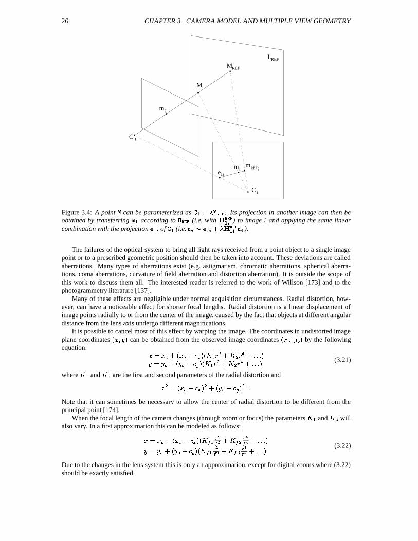
Figure 3.4: A point
can be parameterized as W . A . Its projection in another image can then be
obtained by transferring W according to
(i.e. with W ) to image and applying the same linear
combination with the projection W of W (i.e. ; W . A
W W ).
The failures of the optical system to bring all light rays received from a point object to a single imagepoint or to a prescribed geometric position should then be taken into account. These deviations are calledaberrations. Many types of aberrations exist (e.g. astigmatism, chromatic aberrations, spherical aberra-tions, coma aberrations, curvature of field aberration and distortion aberration). It is outside the scope ofthis work to discuss them all. The interested reader is referred to the work of Willson [173] and to thephotogrammetry literature [137].
Many of these effects are negligible under normal acquisition circumstances. Radial distortion, how-ever, can have a noticeable effect for shorter focal lengths. Radial distortion is a linear displacement ofimage points radially to or from the center of the image, caused by the fact that objects at different angulardistance from the lens axis undergo different magnifications.
It is possible to cancel most of this effect by warping the image. The coordinates in undistorted imageplane coordinates
N 3 8 P can be obtained from the observed image coordinatesN 3 8 P by the following
equation:3& 3 . N 3
P N W , . , . P8 & 8 . N 8
P N W , . , . P (3.21)
where W and
, are the first and second parameters of the radial distortion and
, & N 3 P , . N 8
P , Note that it can sometimes be necessary to allow the center of radial distortion to be different from theprincipal point [174].
When the focal length of the camera changes (through zoom or focus) the parameters W and
, will
also vary. In a first approximation this can be modeled as follows:
3& 3 . N 3 P N
W . , .
P8 & 8 . N 8
P N W .
, . P (3.22)
Due to the changes in the lens system this is only an approximation, except for digital zooms where (3.22)should be exactly satisfied.
3.2. MULTI VIEW GEOMETRY 27
L
M?
R’
R
C
lm
l’m’?
C’
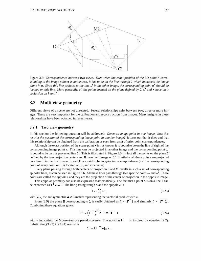
Figure 3.5: Correspondence between two views. Even when the exact position of the 3D point
corre-sponding to the image point is not known, it has to be on the line through
which intersects the image
plane in . Since this line projects to the line E in the other image, the corresponding point E should be
located on this line. More generally, all the points located on the plane defined by
, E and
have their
projection on
and E .
3.2 Multi view geometry
Different views of a scene are not unrelated. Several relationships exist between two, three or more im-ages. These are very important for the calibration and reconstruction from images. Many insights in theserelationships have been obtained in recent years.
3.2.1 Two view geometry
In this section the following question will be addressed: Given an image point in one image, does thisrestrict the position of the corresponding image point in another image? It turns out that it does and thatthis relationship can be obtained from the calibration or even from a set of prior point correspondences.
Although the exact position of the scene point
is not known, it is bound to be on the line of sight of thecorresponding image point . This line can be projected in another image and the corresponding point Eis bound to be on this projected line
E . This is illustrated in Figure 3.5. In fact all the points on the plane
defined by the two projection centers and
have their image on E . Similarly, all these points are projected
on a line
in the first image.
and E are said to be in epipolar correspondence (i.e. the corresponding
point of every point on
is located on E , and vice versa).
Every plane passing through both centers of projection
and E results in such a set of corresponding
epipolar lines, as can be seen in Figure 3.6. All these lines pass through two specific points and E . Thesepoints are called the epipoles, and they are the projection of the center of projection in the opposite image.
This epipolar geometry can also be expressed mathematically. The fact that a point is on a line
canbe expressed as
S &)( . The line passing trough and the epipole is ; 1 5 (3.23)
with 1 5 the antisymmetric matrix representing the vectorial product with .From (3.9) the plane
corresponding to
is easily obtained as
; S and similarly ; E S E .
Combining these equations gives:
E ; E S ] S UZS (3.24)
with indicating the Moore-Penrose pseudo-inverse. The notation U S
is inspired by equation (2.7).Substituting (3.23) in (3.24) results in E ; U S 1 5
28 CHAPTER 3. CAMERA MODEL AND MULTIPLE VIEW GEOMETRY
Cl
l’
L
R
e’e
R’
C’
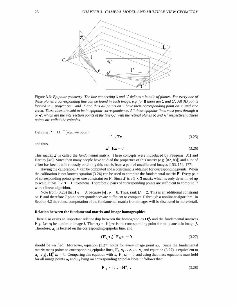
Figure 3.6: Epipolar geometry. The line connecting
and E defines a bundle of planes. For every one of
these planes a corresponding line can be found in each image, e.g. for
these are
and E . All 3D points
located in
project on
and E and thus all points on
have their corresponding point on
E and viceversa. These lines are said to be in epipolar correspondence. All these epipolar lines must pass through or E , which are the intersection points of the line
E with the retinal planes and E respectively. Thesepoints are called the epipoles.
Defining & UZS 1 5 , we obtain E ; (3.25)
and thus, E S &D( (3.26)
This matrix
is called the fundamental matrix. These concepts were introduced by Faugeras [31] andHartley [46]. Since then many people have studied the properties of this matrix (e.g. [82, 83]) and a lot ofeffort has been put in robustly obtaining this matrix from a pair of uncalibrated images [153, 154, 177].
Having the calibration,
can be computed and a constraint is obtained for corresponding points. Whenthe calibration is not known equation (3.26) can be used to compute the fundamental matrix
. Every pair
of corresponding points gives one constraint on
. Since
is a 8 matrix which is only determined upto scale, it has : unknowns. Therefore 8 pairs of corresponding points are sufficient to compute
with a linear algorithm.
Note from (3.25) that & ( , because 1 5 & ( . Thus, rank
& . This is an additional constrainton
and therefore 7 point correspondences are sufficient to compute
through a nonlinear algorithm. InSection 4.2 the robust computation of the fundamental matrix from images will be discussed in more detail.
Relation between the fundamental matrix and image homographies
There also exists an important relationship between the homographies L
and the fundamental matrices L. Let be a point in image . Then ; L is the corresponding point for the plane
in image .
Therefore, is located on the corresponding epipolar line; and,
N L P S &D( (3.27)
should be verified. Moreover, equation (3.27) holds for every image point . Since the fundamentalmatrix maps points to corresponding epipolar lines,
L ; L and equation (3.27) is equivalent to S 1 L 5 &)( . Comparing this equation with S &)( , and using that these equations must holdfor all image points and lying on corresponding epipolar lines, it follows that:
L ; 1 5 L (3.28)
3.2. MULTI VIEW GEOMETRY 29
Let
be a line in image and let
be the plane obtained by back-projecting
into space. If is theimage of a point of this plane projected in image , then the corresponding point in image must be locatedon the corresponding epipolar line (i.e.
L ). Since this point is also located on the line
it can beuniquely determined as the intersection of both (if these lines are not coinciding):
L . Therefore,the homography
is given by 1 5 L . Note that, since the image of the plane
is a line in image ,
this homography is not of full rank. An obvious choice to avoid coincidence of
with the epipolar lines,is ; since this line does certainly not contain the epipole (i.e. S L B&)( ). Consequently,
1 5 L (3.29)
corresponds to the homography of a plane. By combining this result with equations (3.16) and (3.17) onecan conclude that it is always possible to write the projection matrices for two views as
W & 1 \ ( 5, & 1 1 W , 5 W , W , S W , 5 (3.30)
Note that this is an important result, since it means that a projective camera setup can be obtained from thefundamental matrix which can be computed from 7 or more matches between two views. Note also that thisequation has 4 degrees of freedom (i.e. the 3 coefficients of and the arbitrary relative scale between
W ,and W , ). Therefore, this equation can only be used to instantiate a new frame (i.e. an arbitrary projectiverepresentation of the scene) and not to obtain the projection matrices for all the views of a sequence (i.e.compute
). How this can be done is explained in Section 5.2.
3.2.2 Three view geometry
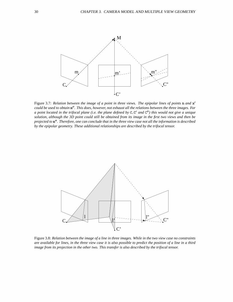
Considering three views it is, of course, possible to group them in pairs and to get the two view relationshipsintroduced in the last section. Using these pairwise epipolar relations, the projection of a point in the thirdimage can be predicted from the coordinates in the first two images. This is illustrated in Figure 3.7. Thepoint in the third image is determined as the intersection of the two epipolar lines. This computation,however, is not always very well conditioned. When the point is located in the trifocal plane (i.e. the planegoing through the three centers of projection), it is completely undetermined.
Fortunately, there are additional constraints between the images of a point in three views. When thecenters of projection are not coinciding, a point can always be reconstructed from two views. This pointthen projects to a unique point in the third image, as can be seen in Figure 3.7, even when this point is lo-cated in the trifocal plane. For two views, no constraint is available to restrict the position of correspondinglines. Indeed, back-projecting a line forms a plane, the intersection of two planes always results in a line.Therefore, no constraint can be obtained from this. But, having three views, the image of the line in thethird view can be predicted from its location in the first two images, as can be seen in Figure 3.8. Similar towhat was derived for two views, there are multi linear relationships relating the positions of points and/orlines in three images [140]. The coefficients of these multi linear relationships can be organized in a tensorwhich describes the relationships between points [135] and lines [49] or any combination thereof [51].Several researchers have worked on methods to compute the trifocal tensor (e.g. see [151, 152]).
The trifocal tensor
is a O tensor. It contains 27 parameters, only 18 of which are independentdue to additional nonlinear constraints. The trilinear relationship for a point is given by the followingequation1:
N E E E E E L E . P &D( (3.31)
Any triplet of corresponding points should satisfy this constraint.A similar constraint applies for lines. Any triplet of corresponding lines should satisfy:
; E E E L 1The Einstein convention is used (i.e. indices that are repeated should be summed over).
30 CHAPTER 3. CAMERA MODEL AND MULTIPLE VIEW GEOMETRY
C
m’ m"m
C’
M
C"
Figure 3.7: Relation between the image of a point in three views. The epipolar lines of points and Ecould be used to obtain E E . This does, however, not exhaust all the relations between the three images. Fora point located in the trifocal plane (i.e. the plane defined by
E and E E ) this would not give a unique
solution, although the 3D point could still be obtained from its image in the first two views and then beprojected to E E . Therefore, one can conclude that in the three view case not all the information is describedby the epipolar geometry. These additional relationships are described by the trifocal tensor.
C"
C’
Cl l"
l’
Figure 3.8: Relation between the image of a line in three images. While in the two view case no constraintsare available for lines, in the three view case it is also possible to predict the position of a line in a thirdimage from its projection in the other two. This transfer is also described by the trifocal tensor.
3.3. CONCLUSION 31
3.2.3 Multi view geometry
Many people have been studying multi view relationships [59, 156, 34]. Without going into detail wewould like to give some intuitive insights to the reader. For a more in depth discussion the reader isreferred to [88].
An image point has 2 degrees of freedom. But , images of a 3D point do not have , degrees offreedom, but only 3. So, there must be , independent constraints between them. For lines, whichalso have 2 degrees of freedom in the image, but 4 in 3D space, , images of a line must satisfy , constraints.
Some more properties of these constraints are explained here. A line can be back-projected into spacelinearly (3.9). A point can be seen as the intersection of two lines. To correspond to a real point or linethe planes resulting from the backprojection must all intersect in a single point or line. This is easilyexpressed in terms of determinants, i.e.
W , & ( for points and that all the Y subdeterminants
of 1 W , 5 should be zero for lines. This explains why the constraints are multi linear, since this is a
property of columns of a determinant. In addition no constraints combining more than 4 images exist,since with 4-vectors (i.e. the representation of the planes) maximum TV determinants can be obtained.The twofocal (i.e. the fundamental matrix) and the trifocal tensors have been discussed in the previousparagraphs, recently Hartley [54] proposed an algorithm for the practical computation of the quadrifocaltensor.
3.3 Conclusion
In this chapter some important concepts were introduced. A geometric description of the image formationprocess was given and the camera projection matrix was introduced. Some important relationships betweenmultiple views were also derived. The insights obtained by carefully studying these properties have shownthat it is possible to retrieve a relative calibration of a two view camera setup from point matches only. Thisis an important result which will be exploited further on to obtain a 3D reconstruction starting from theimages.

32 CHAPTER 3. CAMERA MODEL AND MULTIPLE VIEW GEOMETRY
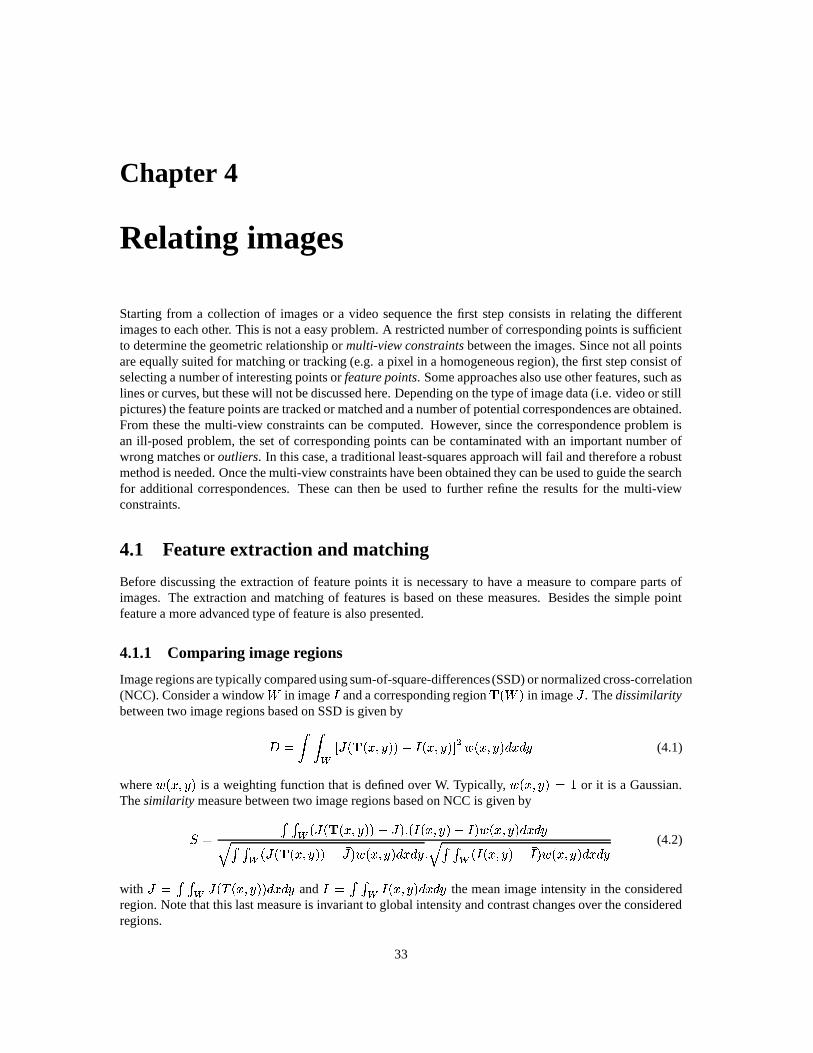
Chapter 4
Relating images
Starting from a collection of images or a video sequence the first step consists in relating the differentimages to each other. This is not a easy problem. A restricted number of corresponding points is sufficientto determine the geometric relationship or multi-view constraints between the images. Since not all pointsare equally suited for matching or tracking (e.g. a pixel in a homogeneous region), the first step consist ofselecting a number of interesting points or feature points. Some approaches also use other features, such aslines or curves, but these will not be discussed here. Depending on the type of image data (i.e. video or stillpictures) the feature points are tracked or matched and a number of potential correspondences are obtained.From these the multi-view constraints can be computed. However, since the correspondence problem isan ill-posed problem, the set of corresponding points can be contaminated with an important number ofwrong matches or outliers. In this case, a traditional least-squares approach will fail and therefore a robustmethod is needed. Once the multi-view constraints have been obtained they can be used to guide the searchfor additional correspondences. These can then be used to further refine the results for the multi-viewconstraints.
4.1 Feature extraction and matching
Before discussing the extraction of feature points it is necessary to have a measure to compare parts ofimages. The extraction and matching of features is based on these measures. Besides the simple pointfeature a more advanced type of feature is also presented.
4.1.1 Comparing image regions
Image regions are typically compared using sum-of-square-differences (SSD) or normalized cross-correlation(NCC). Consider a window % in image and a corresponding region
N % P in image . The dissimilaritybetween two image regions based on SSD is given by & 1 N N 3 8 P P N 3 8 P 5 , N 3 8 P 3 8 (4.1)
where N 3 8 P is a weighting function that is defined over W. Typically, N 3 8 P & or it is a Gaussian.The similarity measure between two image regions based on NCC is given by
& N N N 3 8 P P P N N 3 8 P P N 3 8 P 3 8
N N N 3 8 P P P N 3 8 P 3 8
N N 3 8 P P N 3 8 P 3 8 (4.2)
with 4& N N 3 8 P P 3 8 and &
N 3 8 P 3 8 the mean image intensity in the consideredregion. Note that this last measure is invariant to global intensity and contrast changes over the consideredregions.
33
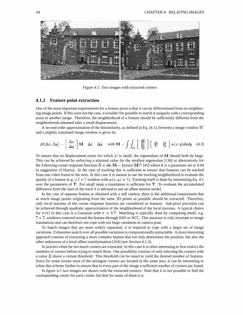
34 CHAPTER 4. RELATING IMAGES
Figure 4.1: Two images with extracted corners
4.1.2 Feature point extraction
One of the most important requirements for a feature point is that it can be differentiated from its neighbor-ing image points. If this were not the case, it wouldn’t be possible to match it uniquely with a correspondingpoint in another image. Therefore, the neighborhood of a feature should be sufficiently different from theneighborhoods obtained after a small displacement.
A second order approximation of the dissimilarity, as defined in Eq. (4.1), between a image window %and a slightly translated image window is given by
N 3 8 P & 3 8 3 8 with &
N 3 8 P 3 8 (4.3)
To ensure that no displacement exists for which
is small, the eigenvalues of
should both be large.This can be achieved by enforcing a minimal value for the smallest eigenvalue [136] or alternatively forthe following corner response function & N trace
P , [45] where is a parameter set to 0.04(a suggestion of Harris). In the case of tracking this is sufficient to ensure that features can be trackedfrom one video frame to the next. In this case it is natural to use the tracking neighborhood to evaluate thequality of a feature (e.g. a
window with N 3 8 P & ). Tracking itself is done by minimizing Eq. 4.1over the parameters of
. For small steps a translation is sufficient for
. To evaluate the accumulated
difference from the start of the track it is advised to use an affine motion model.In the case of separate frames as obtained with a still camera, there is the additional requirement that
as much image points originating from the same 3D points as possible should be extracted. Therefore,only local maxima of the corner response function are considered as features. Sub-pixel precision canbe achieved through quadratic approximation of the neighborhood of the local maxima. A typical choicefor N 3 P in this case is a Gaussian with & ( . Matching is typically done by comparing small, e.g. , windows centered around the feature through SSD or NCC. This measure is only invariant to imagetranslations and can therefore not cope with too large variations in camera pose.
To match images that are more widely separated, it is required to cope with a larger set of imagevariations. Exhaustive search over all possible variations is computationally untractable. A more interestingapproach consists of extracting a more complex feature that not only determines the position, but also theother unknowns of a local affine transformation [164] (see Section 4.1.3).
In practice often far too much corners are extracted. In this case it is often interesting to first restrict thenumbers of corners before trying to match them. One possibility consists of only selecting the corners witha value above a certain threshold. This threshold can be tuned to yield the desired number of features.Since for some scenes most of the strongest corners are located in the same area, it can be interesting torefine this scheme further to ensure that in every part of the image a sufficient number of corners are found.
In figure 4.1 two images are shown with the extracted corners. Note that it is not possible to find thecorresponding corner for each corner, but that for many of them it is.
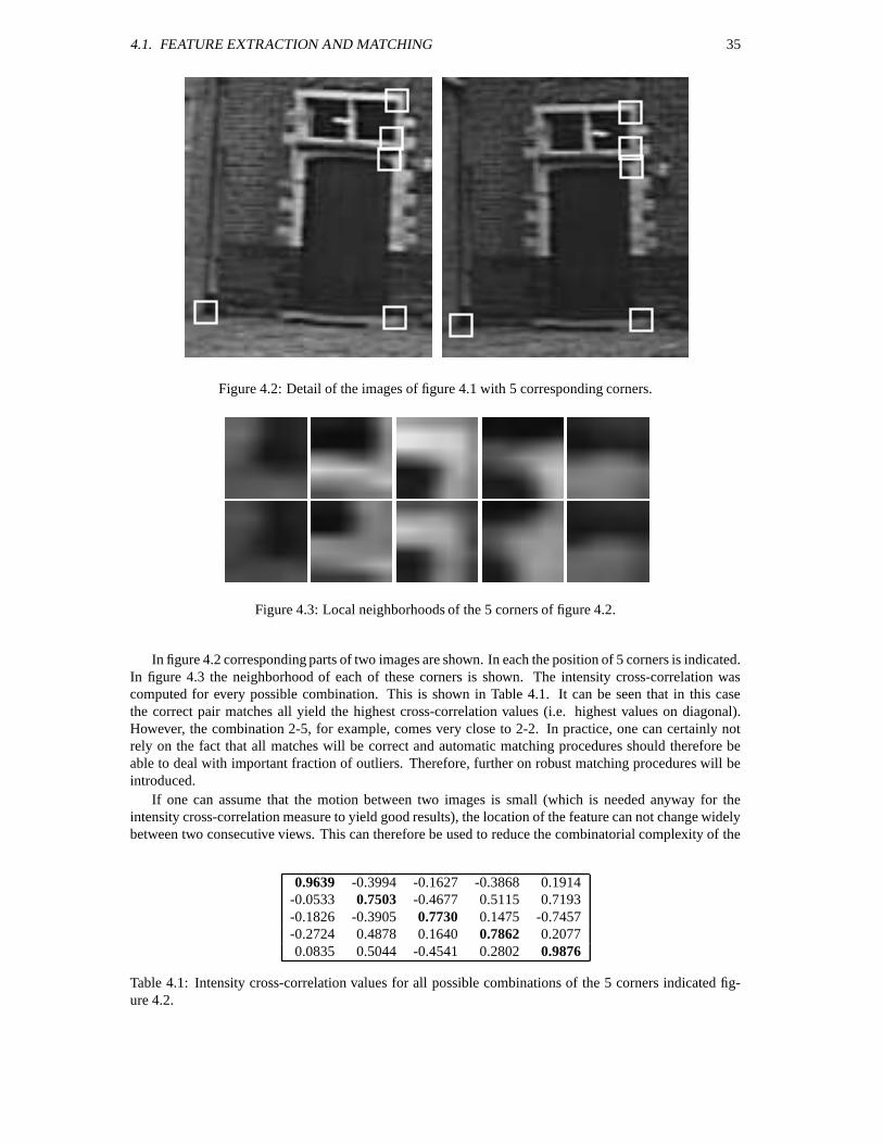
4.1. FEATURE EXTRACTION AND MATCHING 35
Figure 4.2: Detail of the images of figure 4.1 with 5 corresponding corners.
Figure 4.3: Local neighborhoods of the 5 corners of figure 4.2.
In figure 4.2 corresponding parts of two images are shown. In each the position of 5 corners is indicated.In figure 4.3 the neighborhood of each of these corners is shown. The intensity cross-correlation wascomputed for every possible combination. This is shown in Table 4.1. It can be seen that in this casethe correct pair matches all yield the highest cross-correlation values (i.e. highest values on diagonal).However, the combination 2-5, for example, comes very close to 2-2. In practice, one can certainly notrely on the fact that all matches will be correct and automatic matching procedures should therefore beable to deal with important fraction of outliers. Therefore, further on robust matching procedures will beintroduced.
If one can assume that the motion between two images is small (which is needed anyway for theintensity cross-correlation measure to yield good results), the location of the feature can not change widelybetween two consecutive views. This can therefore be used to reduce the combinatorial complexity of the
0.9639 -0.3994 -0.1627 -0.3868 0.1914-0.0533 0.7503 -0.4677 0.5115 0.7193-0.1826 -0.3905 0.7730 0.1475 -0.7457-0.2724 0.4878 0.1640 0.7862 0.20770.0835 0.5044 -0.4541 0.2802 0.9876
Table 4.1: Intensity cross-correlation values for all possible combinations of the 5 corners indicated fig-ure 4.2.
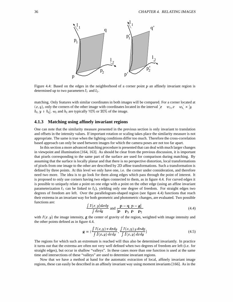
36 CHAPTER 4. RELATING IMAGES
2
q q’
p’2
p’
1
2l2l
ll 1
11p
pp p’
Figure 4.4: Based on the edges in the neighborhood of a corner point an affinely invariant region isdetermined up to two parameters W and , .
matching. Only features with similar coordinates in both images will be compared. For a corner located atN 3 8 P , only the corners of the other image with coordinates located in the interval 1 3 32. 5 1 8 8 . G 5 . and
are typically ( or F( of the image.
4.1.3 Matching using affinely invariant regions
One can note that the similarity measure presented in the previous section is only invariant to translationand offsets in the intensity values. If important rotation or scaling takes place the similarity measure is notappropriate. The same is true when the lighting conditions differ too much. Therefore the cross-correlationbased approach can only be used between images for which the camera poses are not too far apart.
In this section a more advanced matching procedure is presented that can deal with much larger changesin viewpoint and illumination [164, 163]. As should be clear from the previous discussion, it is importantthat pixels corresponding to the same part of the surface are used for comparison during matching. Byassuming that the surface is locally planar and that there is no perspective distortion, local transformationsof pixels from one image to the other are described by 2D affine transformations. Such a transformation isdefined by three points. At this level we only have one, i.e. the corner under consideration, and thereforeneed two more. The idea is to go look for them along edges which pass through the point of interest. Itis proposed to only use corners having two edges connected to them, as in figure 4.4. For curved edges itis possible to uniquely relate a point on one edge with a point on the other edge (using an affine invariantparameterization W can be linked to , ), yielding only one degree of freedom. For straight edges twodegrees of freedom are left. Over the parallelogram-shaped region (see figure 4.4) functions that reachtheir extrema in an invariant way for both geometric and photometric changes, are evaluated. Two possiblefunctions are: N 3 8 P 3 8 3 8 and
W , (4.4)
with N 3 8 P the image intensity, the center of gravity of the region, weighted with image intensity andthe other points defined as in figure 4.4.
& N N 3 8 P 3 3 8 N 3 8 P 3 8 N 3 8 P 8 3 8 N 3 8 P 3 8 P (4.5)
The regions for which such an extremum is reached will thus also be determined invariantly. In practiceit turns out that the extrema are often not very well defined when two degrees of freedom are left (i.e. forstraight edges), but occur in shallow “valleys”. In these cases more than one function is used at the sametime and intersections of these “valleys” are used to determine invariant regions.
Now that we have a method at hand for the automatic extraction of local, affinely invariant imageregions, these can easily be described in an affinely invariant way using moment invariants [166]. As in the
4.2. TWO VIEW GEOMETRY COMPUTATION 37
region finding steps, invariance both under affine geometric changes and linear photometric changes, withdifferent offsets and different scale factors for each of the three color bands, is considered.
For each region, a feature vector of moment invariance is composed. These can be compared quiteefficiently with the invariant vectors computed for other regions, using a hashing-technique. It can beinteresting to take the region type (curved or straight edges? Extrema of which function?) into accountas well. Once the corresponding regions have been identified, the cross-correlation between them (afternormalization to a square reference region) is computed as a final check to reject false matches.
4.2 Two view geometry computation
As was seen in Section 3.2.1, even for an arbitrary geometric structure, the projections of points in twoviews contains some structure. Finding back this structure is not only very interesting since it is equivalentto the projective calibration of the camera for the two views, but also allows to simplify the search formore matches since these have to satisfy the epipolar constraint. As will be seen further it also allows toeliminate most of the outliers from the matches.
4.2.1 Eight-point algorithm
The two view structure is equivalent to the fundamental matrix. Since the fundamental matrix
is a Tmatrix determined up to an arbitrary scale factor, 8 equations are required to obtain a unique solution. Thesimplest way to compute the fundamental matrix consists of using Equation (3.26). This equation can berewritten under the following form:
393E 8 3E 3E 3 8 E 8$8 E 8 E 3 8 & ( (4.6)
with & 1 3 8 5 S E &D1 3E 8 E 5 S and & 1 W W W , W , W , , , W , 5 S a vector containing theelements of the fundamental matrix
. By stacking eight of these equations in a matrix
the following
equation is obtained: & ( (4.7)
This system of equation is easily solved by Singular Value Decomposition (SVD) [43]. Applying SVD to
yields the decomposition S
with and orthonormal matrices and a diagonal matrix containingthe singular values. These singular values are positive and in decreasing order. Therefore in our case is guaranteed to be identically zero (8 equations for 9 unknowns) and thus the last column of is thecorrect solution (at least as long as the eight equations are linearly independent, which is equivalent to allother singular values being non-zero).
It is trivial to reconstruct the fundamental matrix
from the solution vector . However, in the presenceof noise, this matrix will not satisfy the rank-2 constraint. This means that there will not be real epipolesthrough which all epipolar lines pass, but that these will be “smeared out” to a small region. A solutionto this problem is to obtain
as the closest rank-2 approximation of the solution coming out of the linear
equations.
4.2.2 Seven-point algorithm
In fact the two view structure (or the fundamental matrix) only has seven degrees of freedom. If one isprepared to solve non-linear equations, seven points must thus be sufficient to solve for it. In this case therank-2 constraint must be enforced during the computations.
A similar approach as in the previous section can be followed to characterize the right null-space of thesystem of linear equations originating from the seven point correspondences. This space can be parameter-ized as follows W . A , or
W . A , with W and , being the two last columns of (obtained throughSVD) and
W respectively, the corresponding matrices. The rank-2 constraint is then written as
N W . A ,P &D A .1 , A , .1 W A .1 &D( (4.8)
38 CHAPTER 4. RELATING IMAGES
which is a polynomial of degree 3 in A . This can simply be solved analytically. There are always 1 or 3 realsolutions. The special case
W (which is not covered by this parameterization) is easily checked separately,i.e. it should have rank-2. If more than one solution is obtained then more points are needed to obtain thetrue fundamental matrix.
4.2.3 More points...
It is clear that when more point matches are available the redundancy should be used to minimize the effectof the noise. The eight-point algorithm can easily be extended to be used with more points. In this case thematrix
of equation 4.7 will be much bigger, it will have one row per point match. The solution can be
obtained in the same way, but in this case the last singular value will not be perfectly equal to zero. It hasbeen pointed out [52] that in practice it is very important to normalize the equations. This is for exampleachieved by transforming the image to the interval 1 5 1 5 so that all elements of the matrix
are of the same order of magnitude.
Even then the error that is minimized is an algebraic error which has nor real “physical” meaning. Itis always better to minimize a geometrically meaningful criterion. The error measure that immediatelycomes to mind is the distance between the points and the epipolar lines. Assuming that the noise on everyfeature point is independent zero-mean Gaussian with the same sigma for all points, the minimization ofthe following criterion yields a maximum likelihood solution:
N P & L YN E P , . YN S E P , (4.9)
withYN P the orthogonal distance between the point and the line
. This criterion can be minimized
through a Levenberg-Marquard algorithm [122]. The results obtained through linear least-squares can beused for initialization.
4.2.4 Robust algorithm
The most important problem with the previous approaches is that they can not cope with outliers. If the setof matches is contaminated with even a small set of outliers, the result will probably be unusable. This istypical for all types of least-squares approaches (even non-linear ones). The problem is that the quadraticpenalty (which is optimal for Gaussian noise) allows a single outlier being very far apart from the truesolution to completely bias the final result.
The problem is that it is very hard to segment the set of matches in inliers and outliers before havingthe correct solution. The outliers could have such a disastrous effect on the least-square computationsthat almost no points would be classified as inliers (see Torr [154] for a more in depth discussion of thisproblem).
A solution to this problem was proposed by Fischler and Bolles [35] (see also [127] for more detailson robust statistics). Their algorithm is called RANSAC (RANdom SAmpling Consensus) and it can beapplied to all kinds of problems.
Let us take a subset of the data and compute a solution from it. If were are lucky and there are nooutliers in our set, the solution will be correct and we will be able to correctly segment the data in inliersand outliers. Of course, we can not rely on being lucky. However, by repeating this procedure withrandomly selected subsets, in the end we should end up with the correct solution. The correct solution isidentified as the solution with the largest support (i.e. having the largest number of inliers).
Matches are considered inliers if they are not more than pixels away from their epipolar lines,with characterizing the amount of noise on the position of the features. In practice is hard to estimateand one could just set it to 0.5 or 1 pixel, for example.
The remaining question is of course ’how many samples should be taken?’. Ideally one could try outevery possible subset, but this is usually computationally infeasible, so one takes the number of samples sufficiently high to give a probability in excess of that a good subsample was selected. Theexpression for this probability is [127]
& N N P P > (4.10)

4.2. TWO VIEW GEOMETRY COMPUTATION 39
5% 10% 20% 30% 40% 50% 60% 70% 80%3 5 13 35 106 382 1827 13692 233963
Table 4.2: The number of 7-point samples required to ensure ( for a given fraction of outliers.
Step 1. Extract features
Step 2. Compute a set of potential matches
Step 3. While N ,X P do
step 3.1 select minimal sample (7 matches)
step 3.2 compute solutions for F
step 3.3 determine inliers
step 4. Refine F based on all inliers
step 5. Look for additional matches
step 6. Refine F based on all correct matches
Table 4.3: Overview of the two-view geometry computation algorithm.
where is the fraction of outliers, and the number of features in each sample. In the case of the funda-mental matrix &
. Table 4.2 gives the required number of samples for a few values of . The algorithmcan easily deal with up to F( outliers, above this the required number of samples becomes very high.
One approach is to decide a priori which level of outlier contamination the algorithm should deal withand set the number of samples accordingly (e.g. coping with up to F( outliers implies 382 samples).
Often a lower percentage of outliers is present in the data and the correct solution will already havebeen found after much fewer samples. Assume that sample 57 yields a solution with
( of consistentmatches, in this case one could decide to stop at sample 106, being sure -at least for - not to havemissed any bigger set of inliers.
Once the set of matches has been correctly segmented in inliers and outliers, the solution can be refinedusing all the inliers. The procedure of Section 4.2.3 can be used for this. Table 4.3 summarizes the robustapproach to the determination of the two-view geometry. Once the epipolar geometry has been computed itcan be used to guide the matching towards additional matches. At this point only features being in epipolarcorrespondence should be considered for matching. For a corner in one image, only the corners of the otherimage that are within a small region (1 or 2 pixels) around the corresponding epipolar line, are consideredfor matching. At this point the initial coordinate interval that was used for matching can be relaxed. Byreducing the number of potential matches, the ambiguity is reduced and a number of additional matchesare obtained. These can not only be used to refine the solution even further, but will be very useful furtheron in solving the structure from motion problem where it is important that tracked features survive as longas possible in the sequence.
4.2.5 Degenerate case
The computation of the two-view geometry requires that the matches originate from a 3D scene and thatthe motion is more than a pure rotation. If the observed scene is planar, the fundamental matrix is onlydetermined up to three degrees of freedom. The same is true when the camera motion is a pure rotation.
40 CHAPTER 4. RELATING IMAGES
In this last case -only having one center of projection- depth can not be observed. In the absence of noisethe detection of these degenerate cases would not be too hard. Starting from real -and thus noisy- data, theproblem is much harder since the remaining degrees of freedom in the equations are then determined bynoise.
A solution to this problem has been proposed by Torr et al. [155]. The methods will try to fit differentmodels to the data and the one explaining the data best will be selected. The approach is based on anextension of Akaike’s information criterion [1] proposed by Kanatani [64]. It is outside the scope of thistext to describe this method into details. Therefore only the key idea will briefly be sketched here.
Different models are evaluated. In this case the fundamental matrix (corresponding to a 3D sceneand more than a pure rotation), a general homography (corresponding to a planar scene) and a rotation-induced homography are computed. Selecting the model with the smallest residual would always yield themost general model. Akaike’s principle consist of taking into account the effect of the additional degreesof freedom (which when not needed by the structure of the data end up fitting the noise) on the expectedresidual. This boils down to adding a penalty to the observed residuals in function of the number of degreesof freedom of the model. This makes a fair comparison between the different models feasible.
4.3 Three and four view geometry computation
It is possible to determine the three or four view geometry in a similar way to the two view geometrycomputation explained in the previous section. More details on these concepts can be found in Section 3.2.Since the points satisfying the three or four view geometry certainly must satisfy the two view geometry,it is often interesting to have a hierarchical approach. In this case the two view geometry is estimatedfirst from consecutive views. Then triplet matches are inferred by comparing two consecutive sets of pair-matches. These triplets are then used in a robust approach similar to the method presented in Section 4.2.4.In this case only 6 triplets of points are needed. A similar approach is possible for the four view geometry.
The method to recover structure and motion presented in the next chapter only relies on the two viewgeometry. Therefore the interested reader is referred to the literature for more details on the direct compu-tation of three and four view geometric relations. Many authors studied different approaches to computemulti view relations (e.g. [135, 51]). Torr and Zisserman [151] have proposed a robust approach to thecomputation of the three view geometry. Hartley [54] proposed a method to compute the four view geom-etry.
Chapter 5
Structure and motion
In the previous section it was seen how different views could be related to each other. In this sectionthe relation between the views and the correspondences between the features will be used to retrieve thestructure of the scene and the motion of the camera. This problem is called Structure and Motion.
The approach that is proposed here extends [7, 67] by being fully projective and therefore not de-pendent on the quasi-euclidean initialization. This was achieved by carrying out all measurements in theimages. This approach provides an alternative for the triplet-based approach proposed in [36]. An image-based measure that is able to obtain a qualitative distance between viewpoints is also proposed to supportinitialization and determination of close views (independently of the actual projective frame).
At first two images are selected and an initial reconstruction frame is set-up. Then the pose of thecamera for the other views is determined in this frame and each time the initial reconstruction is refinedand extended. In this way the pose estimation of views that have no common features with the referenceviews also becomes possible. Typically, a view is only matched with its predecessor in the sequence. Inmost cases this works fine, but in some cases (e.g. when the camera moves back and forth) it can beinteresting to also relate a new view to a number of additional views. Once the structure and motion hasbeen determined for the whole sequence, the results can be refined through a projective bundle adjustment.Then the ambiguity will be restricted to metric through self-calibration. Finally, a metric bundle adjustmentis carried out to obtain an optimal estimation of the structure and motion.
5.1 Initial structure and motion
The first step consists of selecting two views that are suited for initializing the sequential structure andmotion computation. On the one hand it is important that sufficient features are matched between theseviews, on the other hand the views should not be too close to each other so that the initial structure iswell-conditioned. The first of these criterions is easy to verify, the second one is harder in the uncalibratedcase. The image-based distance that we propose is the median distance between points transferred throughan average planar-homography and the corresponding points in the target image:
median YN E P (5.1)
This planar-homography H is determined as follows from the matches between the two views:
&21 5 . S> . with >. & argmin
L YN N 1 5 . S P E P , (5.2)
In practice the selection of the initial frame can be done by maximizing the product of the number ofmatches and the image-based distance defined above. When features are matched between sparse views,the evaluation can be restricted to consecutive frames. However, when features are tracked over a videosequence, it is important to consider views that are further apart in the sequence.
41
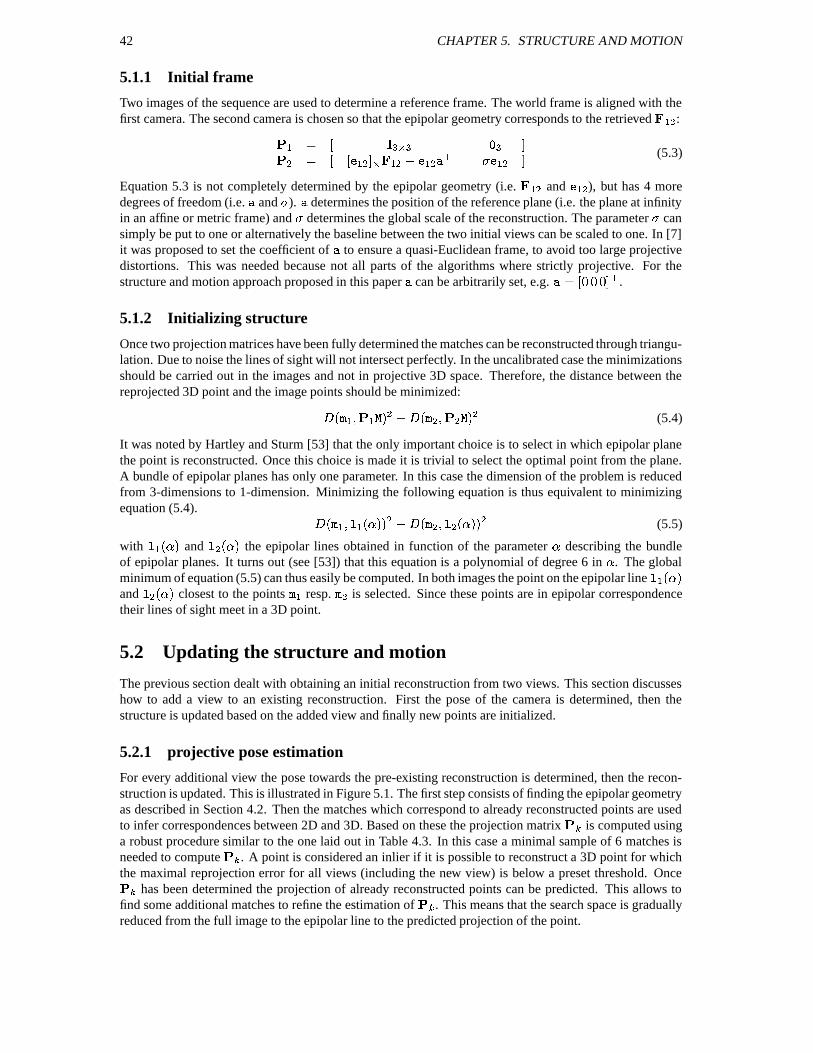
42 CHAPTER 5. STRUCTURE AND MOTION
5.1.1 Initial frame
Two images of the sequence are used to determine a reference frame. The world frame is aligned with thefirst camera. The second camera is chosen so that the epipolar geometry corresponds to the retrieved
W , : W & 1 \ 5, & 1 1 W , 5 W , . W , S W , 5 (5.3)
Equation 5.3 is not completely determined by the epipolar geometry (i.e. W , and W , ), but has 4 more
degrees of freedom (i.e. and ). determines the position of the reference plane (i.e. the plane at infinityin an affine or metric frame) and determines the global scale of the reconstruction. The parameter cansimply be put to one or alternatively the baseline between the two initial views can be scaled to one. In [7]it was proposed to set the coefficient of to ensure a quasi-Euclidean frame, to avoid too large projectivedistortions. This was needed because not all parts of the algorithms where strictly projective. For thestructure and motion approach proposed in this paper can be arbitrarily set, e.g. & 1 ( ( ( 5 S .
5.1.2 Initializing structure
Once two projection matrices have been fully determined the matches can be reconstructed through triangu-lation. Due to noise the lines of sight will not intersect perfectly. In the uncalibrated case the minimizationsshould be carried out in the images and not in projective 3D space. Therefore, the distance between thereprojected 3D point and the image points should be minimized:YN W W P , . YN , , P , (5.4)
It was noted by Hartley and Sturm [53] that the only important choice is to select in which epipolar planethe point is reconstructed. Once this choice is made it is trivial to select the optimal point from the plane.A bundle of epipolar planes has only one parameter. In this case the dimension of the problem is reducedfrom 3-dimensions to 1-dimension. Minimizing the following equation is thus equivalent to minimizingequation (5.4). N W W N P P , . YN , , N P P , (5.5)
with W N P and
,N P the epipolar lines obtained in function of the parameter describing the bundle
of epipolar planes. It turns out (see [53]) that this equation is a polynomial of degree 6 in . The globalminimum of equation (5.5) can thus easily be computed. In both images the point on the epipolar line
W N Pand
,N P closest to the points W resp. , is selected. Since these points are in epipolar correspondence
their lines of sight meet in a 3D point.
5.2 Updating the structure and motion
The previous section dealt with obtaining an initial reconstruction from two views. This section discusseshow to add a view to an existing reconstruction. First the pose of the camera is determined, then thestructure is updated based on the added view and finally new points are initialized.
5.2.1 projective pose estimation
For every additional view the pose towards the pre-existing reconstruction is determined, then the recon-struction is updated. This is illustrated in Figure 5.1. The first step consists of finding the epipolar geometryas described in Section 4.2. Then the matches which correspond to already reconstructed points are usedto infer correspondences between 2D and 3D. Based on these the projection matrix
is computed usinga robust procedure similar to the one laid out in Table 4.3. In this case a minimal sample of 6 matches isneeded to compute
. A point is considered an inlier if it is possible to reconstruct a 3D point for whichthe maximal reprojection error for all views (including the new view) is below a preset threshold. Once has been determined the projection of already reconstructed points can be predicted. This allows tofind some additional matches to refine the estimation of
. This means that the search space is graduallyreduced from the full image to the epipolar line to the predicted projection of the point.
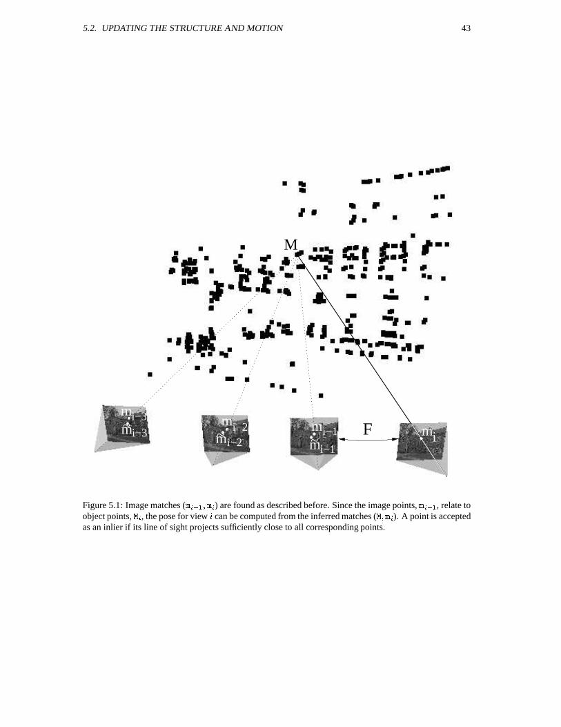
5.2. UPDATING THE STRUCTURE AND MOTION 43
mi
i−3 mi−2 mi−1
M
mFi−3m
mi−2 mi−1~
~~
Figure 5.1: Image matches ( UZW ) are found as described before. Since the image points, UXW , relate toobject points,
, the pose for view can be computed from the inferred matches (
). A point is acceptedas an inlier if its line of sight projects sufficiently close to all corresponding points.
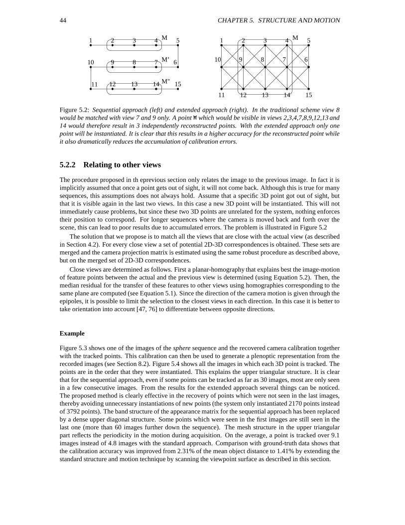
44 CHAPTER 5. STRUCTURE AND MOTION
15141312
1 5432
8
541
10
151413
7
M
M"
M
M’9
12
610
32
11
11
6789
Figure 5.2: Sequential approach (left) and extended approach (right). In the traditional scheme view 8would be matched with view 7 and 9 only. A point
which would be visible in views 2,3,4,7,8,9,12,13 and
14 would therefore result in 3 independently reconstructed points. With the extended approach only onepoint will be instantiated. It is clear that this results in a higher accuracy for the reconstructed point whileit also dramatically reduces the accumulation of calibration errors.
5.2.2 Relating to other views
The procedure proposed in th eprevious section only relates the image to the previous image. In fact it isimplicitly assumed that once a point gets out of sight, it will not come back. Although this is true for manysequences, this assumptions does not always hold. Assume that a specific 3D point got out of sight, butthat it is visible again in the last two views. In this case a new 3D point will be instantiated. This will notimmediately cause problems, but since these two 3D points are unrelated for the system, nothing enforcestheir position to correspond. For longer sequences where the camera is moved back and forth over thescene, this can lead to poor results due to accumulated errors. The problem is illustrated in Figure 5.2
The solution that we propose is to match all the views that are close with the actual view (as describedin Section 4.2). For every close view a set of potential 2D-3D correspondences is obtained. These sets aremerged and the camera projection matrix is estimated using the same robust procedure as described above,but on the merged set of 2D-3D correspondences.
Close views are determined as follows. First a planar-homography that explains best the image-motionof feature points between the actual and the previous view is determined (using Equation 5.2). Then, themedian residual for the transfer of these features to other views using homographies corresponding to thesame plane are computed (see Equation 5.1). Since the direction of the camera motion is given through theepipoles, it is possible to limit the selection to the closest views in each direction. In this case it is better totake orientation into account [47, 76] to differentiate between opposite directions.
Example
Figure 5.3 shows one of the images of the sphere sequence and the recovered camera calibration togetherwith the tracked points. This calibration can then be used to generate a plenoptic representation from therecorded images (see Section 8.2). Figure 5.4 shows all the images in which each 3D point is tracked. Thepoints are in the order that they were instantiated. This explains the upper triangular structure. It is clearthat for the sequential approach, even if some points can be tracked as far as 30 images, most are only seenin a few consecutive images. From the results for the extended approach several things can be noticed.The proposed method is clearly effective in the recovery of points which were not seen in the last images,thereby avoiding unnecessary instantiations of new points (the system only instantiated 2170 points insteadof 3792 points). The band structure of the appearance matrix for the sequential approach has been replacedby a dense upper diagonal structure. Some points which were seen in the first images are still seen in thelast one (more than 60 images further down the sequence). The mesh structure in the upper triangularpart reflects the periodicity in the motion during acquisition. On the average, a point is tracked over 9.1images instead of 4.8 images with the standard approach. Comparison with ground-truth data shows thatthe calibration accuracy was improved from 2.31% of the mean object distance to 1.41% by extending thestandard structure and motion technique by scanning the viewpoint surface as described in this section.
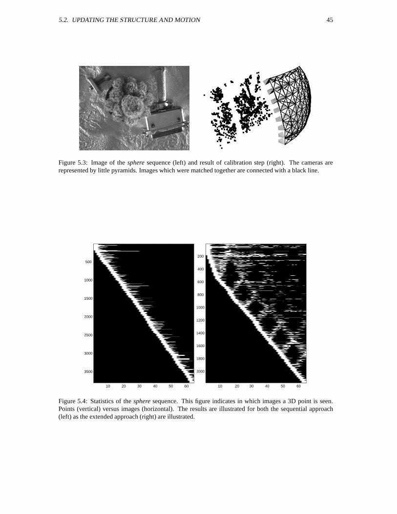
5.2. UPDATING THE STRUCTURE AND MOTION 45
Figure 5.3: Image of the sphere sequence (left) and result of calibration step (right). The cameras arerepresented by little pyramids. Images which were matched together are connected with a black line.
10 20 30 40 50 60
500
1000
1500
2000
2500
3000
3500
10 20 30 40 50 60
200
400
600
800
1000
1200
1400
1600
1800
2000
Figure 5.4: Statistics of the sphere sequence. This figure indicates in which images a 3D point is seen.Points (vertical) versus images (horizontal). The results are illustrated for both the sequential approach(left) as the extended approach (right) are illustrated.
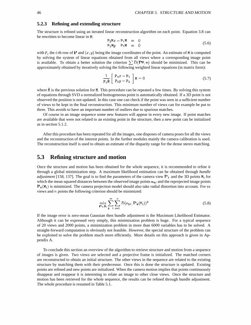
46 CHAPTER 5. STRUCTURE AND MOTION
5.2.3 Refining and extending structure
The structure is refined using an iterated linear reconstruction algorithm on each point. Equation 3.8 canbe rewritten to become linear in
: 3 W & ( 8
, & ( (5.6)
with
the -th row of
andN 3 8 P being the image coordinates of the point. An estimate of
is computed
by solving the system of linear equations obtained from all views where a corresponding image pointis available. To obtain a better solution the criterion K YN P should be minimized. This can beapproximately obtained by iteratively solving the following weighted linear equations (in matrix form):
3 W 8
, &D( (5.7)
where
is the previous solution for
. This procedure can be repeated a few times. By solving this systemof equations through SVD a normalized homogeneous point is automatically obtained. If a 3D point is notobserved the position is not updated. In this case one can check if the point was seen in a sufficient numberof views to be kept in the final reconstruction. This minimum number of views can for example be put tothree. This avoids to have an important number of outliers due to spurious matches.
Of course in an image sequence some new features will appear in every new image. If point matchesare available that were not related to an existing point in the structure, then a new point can be initializedas in section 5.1.2.
After this procedure has been repeated for all the images, one disposes of camera poses for all the viewsand the reconstruction of the interest points. In the further modules mainly the camera calibration is used.The reconstruction itself is used to obtain an estimate of the disparity range for the dense stereo matching.
5.3 Refining structure and motion
Once the structure and motion has been obtained for the whole sequence, it is recommended to refine itthrough a global minimization step. A maximum likelihood estimation can be obtained through bundleadjustment [158, 137]. The goal is to find the parameters of the camera view
and the 3D points
forwhich the mean squared distances between the observed image points and the reprojected image points N P is minimized. The camera projection model should also take radial distortion into account. For views and , points the following criterion should be minimized:
>L M W
.L M WYN N P P , (5.8)
If the image error is zero-mean Gaussian then bundle adjustment is the Maximum Likelihood Estimator.Although it can be expressed very simply, this minimization problem is huge. For a typical sequenceof 20 views and 2000 points, a minimization problem in more than 6000 variables has to be solved. Astraight-forward computation is obviously not feasible. However, the special structure of the problem canbe exploited to solve the problem much more efficiently. More details on this approach is given in Ap-pendix A.
To conclude this section an overview of the algorithm to retrieve structure and motion from a sequenceof images is given. Two views are selected and a projective frame is initialized. The matched cornersare reconstructed to obtain an initial structure. The other views in the sequence are related to the existingstructure by matching them with their predecessor. Once this is done the structure is updated. Existingpoints are refined and new points are initialized. When the camera motion implies that points continuouslydisappear and reappear it is interesting to relate an image to other close views. Once the structure andmotion has been retrieved for the whole sequence, the results can be refined through bundle adjustment.The whole procedure is resumed in Table 5.1.

5.3. REFINING STRUCTURE AND MOTION 47
Step 1. Match or track points over the whole image sequence.
Step 2. Initialize the structure and motion recovery
step 2.1. Select two views that are suited for initialization.
step 2.2. Relate these views by computing the two view geometry.
step 2.3. Set up the initial frame.
step 2.4. Reconstruct the initial structure.
Step 3. For every additional view
step 3.1. Infer matches to the structure and compute the camera pose using arobust algorithm.
step 3.2. Refine the existing structure.
step 3.3. (optional) For already computed views which are “close”
3.4.1. Relate this view with the current view by finding feature matches andcomputing the two view geometry.
3.4.2. Infer new matches to the structure based on the computed matches andadd these to the list used in step 3.1.
Refine the pose from all the matches using a robust algorithm.
step 3.5. Initialize new structure points.
Step 4. Refine the structure and motion through bundle adjustment.
Table 5.1: Overview of the projective structure and motion algorithm.
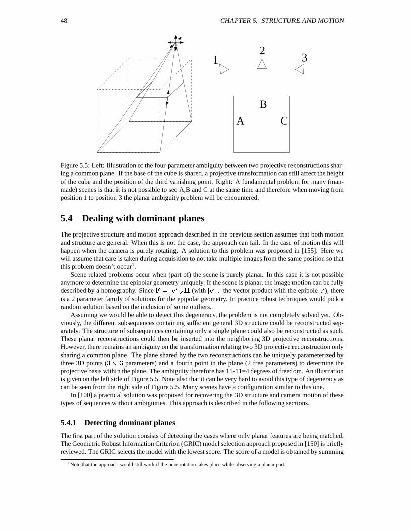
48 CHAPTER 5. STRUCTURE AND MOTION
CA
B
312
Figure 5.5: Left: Illustration of the four-parameter ambiguity between two projective reconstructions shar-ing a common plane. If the base of the cube is shared, a projective transformation can still affect the heightof the cube and the position of the third vanishing point. Right: A fundamental problem for many (man-made) scenes is that it is not possible to see A,B and C at the same time and therefore when moving fromposition 1 to position 3 the planar ambiguity problem will be encountered.
5.4 Dealing with dominant planes
The projective structure and motion approach described in the previous section assumes that both motionand structure are general. When this is not the case, the approach can fail. In the case of motion this willhappen when the camera is purely rotating. A solution to this problem was proposed in [155]. Here wewill assume that care is taken during acquisition to not take multiple images from the same position so thatthis problem doesn’t occur1.
Scene related problems occur when (part of) the scene is purely planar. In this case it is not possibleanymore to determine the epipolar geometry uniquely. If the scene is planar, the image motion can be fullydescribed by a homography. Since
& 1 E 5 (with 1 E 5 the vector product with the epipole E ), thereis a 2 parameter family of solutions for the epipolar geometry. In practice robust techniques would pick arandom solution based on the inclusion of some outliers.
Assuming we would be able to detect this degeneracy, the problem is not completely solved yet. Ob-viously, the different subsequences containing sufficient general 3D structure could be reconstructed sep-arately. The structure of subsequences containing only a single plane could also be reconstructed as such.These planar reconstructions could then be inserted into the neighboring 3D projective reconstructions.However, there remains an ambiguity on the transformation relating two 3D projective reconstruction onlysharing a common plane. The plane shared by the two reconstructions can be uniquely parameterized bythree 3D points ( C parameters) and a fourth point in the plane (2 free parameters) to determine theprojective basis within the plane. The ambiguity therefore has 15-11=4 degrees of freedom. An illustrationis given on the left side of Figure 5.5. Note also that it can be very hard to avoid this type of degeneracy ascan be seen from the right side of Figure 5.5. Many scenes have a configuration similar to this one.
In [100] a practical solution was proposed for recovering the 3D structure and camera motion of thesetypes of sequences without ambiguities. This approach is described in the following sections.
5.4.1 Detecting dominant planes
The first part of the solution consists of detecting the cases where only planar features are being matched.The Geometric Robust Information Criterion (GRIC) model selection approach proposed in [150] is brieflyreviewed. The GRIC selects the model with the lowest score. The score of a model is obtained by summing
1Note that the approach would still work if the pure rotation takes place while observing a planar part.
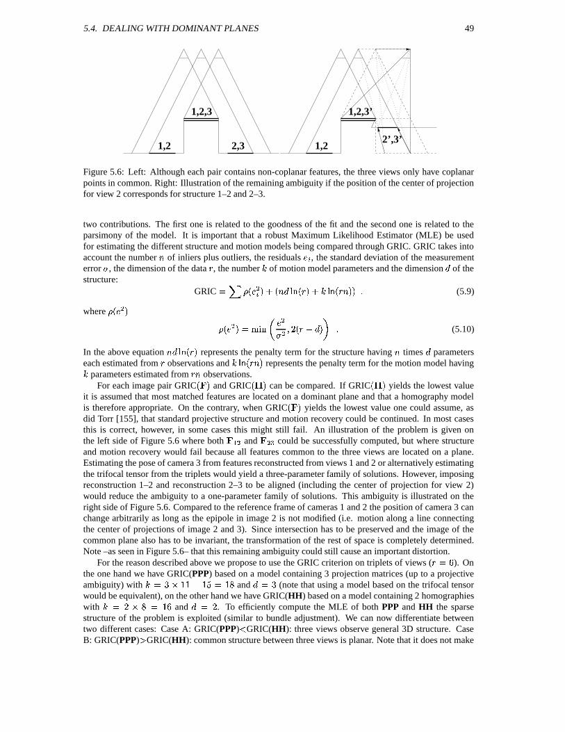
5.4. DEALING WITH DOMINANT PLANES 49
1,2 2,3
1,2,3
1,22’,3’
1,2,3’
Figure 5.6: Left: Although each pair contains non-coplanar features, the three views only have coplanarpoints in common. Right: Illustration of the remaining ambiguity if the position of the center of projectionfor view 2 corresponds for structure 1–2 and 2–3.
two contributions. The first one is related to the goodness of the fit and the second one is related to theparsimony of the model. It is important that a robust Maximum Likelihood Estimator (MLE) be usedfor estimating the different structure and motion models being compared through GRIC. GRIC takes intoaccount the number , of inliers plus outliers, the residuals , the standard deviation of the measurementerror , the dimension of the data
, the number of motion model parameters and the dimension
of the
structure:GRIC & L * N , P . N , N P . N , P P (5.9)
where * N , P* N , P &
, , N P (5.10)
In the above equation , N P represents the penalty term for the structure having , times
parameterseach estimated from
observations and N , P represents the penalty term for the motion model having
parameters estimated from , observations.
For each image pair GRICN P
and GRICN P
can be compared. If GRICN P
yields the lowest valueit is assumed that most matched features are located on a dominant plane and that a homography modelis therefore appropriate. On the contrary, when GRIC
N Pyields the lowest value one could assume, as
did Torr [155], that standard projective structure and motion recovery could be continued. In most casesthis is correct, however, in some cases this might still fail. An illustration of the problem is given onthe left side of Figure 5.6 where both
W , and, could be successfully computed, but where structure
and motion recovery would fail because all features common to the three views are located on a plane.Estimating the pose of camera 3 from features reconstructed from views 1 and 2 or alternatively estimatingthe trifocal tensor from the triplets would yield a three-parameter family of solutions. However, imposingreconstruction 1–2 and reconstruction 2–3 to be aligned (including the center of projection for view 2)would reduce the ambiguity to a one-parameter family of solutions. This ambiguity is illustrated on theright side of Figure 5.6. Compared to the reference frame of cameras 1 and 2 the position of camera 3 canchange arbitrarily as long as the epipole in image 2 is not modified (i.e. motion along a line connectingthe center of projections of image 2 and 3). Since intersection has to be preserved and the image of thecommon plane also has to be invariant, the transformation of the rest of space is completely determined.Note –as seen in Figure 5.6– that this remaining ambiguity could still cause an important distortion.
For the reason described above we propose to use the GRIC criterion on triplets of views ( &
). Onthe one hand we have GRIC(PPP) based on a model containing 3 projection matrices (up to a projectiveambiguity) with & & and
& (note that using a model based on the trifocal tensorwould be equivalent), on the other hand we have GRIC(HH) based on a model containing 2 homographieswith & V & and
& . To efficiently compute the MLE of both PPP and HH the sparsestructure of the problem is exploited (similar to bundle adjustment). We can now differentiate betweentwo different cases: Case A: GRIC(PPP)
GRIC(HH): three views observe general 3D structure. Case
B: GRIC(PPP) GRIC(HH): common structure between three views is planar. Note that it does not make
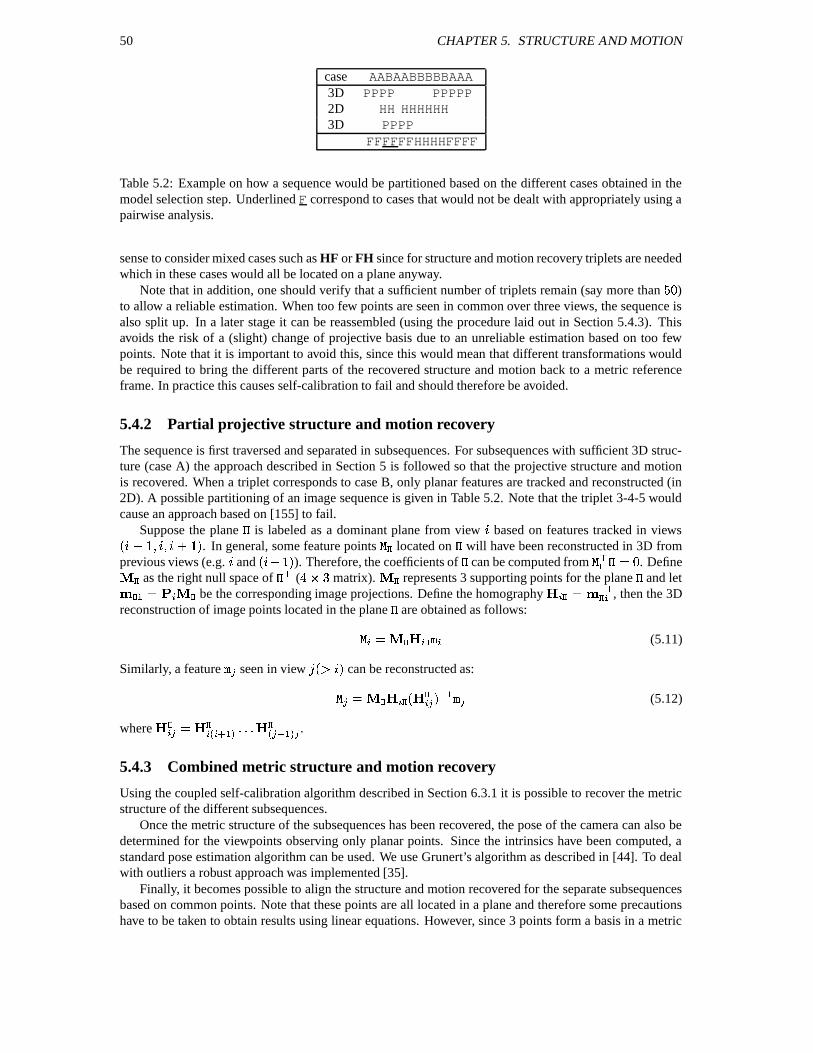
50 CHAPTER 5. STRUCTURE AND MOTION
case AABAABBBBBAAA3D PPPP PPPPP2D HH HHHHHH3D PPPP
FFFFFFHHHHFFFF
Table 5.2: Example on how a sequence would be partitioned based on the different cases obtained in themodel selection step. Underlined F correspond to cases that would not be dealt with appropriately using apairwise analysis.
sense to consider mixed cases such as HF or FH since for structure and motion recovery triplets are neededwhich in these cases would all be located on a plane anyway.
Note that in addition, one should verify that a sufficient number of triplets remain (say more than F( )to allow a reliable estimation. When too few points are seen in common over three views, the sequence isalso split up. In a later stage it can be reassembled (using the procedure laid out in Section 5.4.3). Thisavoids the risk of a (slight) change of projective basis due to an unreliable estimation based on too fewpoints. Note that it is important to avoid this, since this would mean that different transformations wouldbe required to bring the different parts of the recovered structure and motion back to a metric referenceframe. In practice this causes self-calibration to fail and should therefore be avoided.
5.4.2 Partial projective structure and motion recovery
The sequence is first traversed and separated in subsequences. For subsequences with sufficient 3D struc-ture (case A) the approach described in Section 5 is followed so that the projective structure and motionis recovered. When a triplet corresponds to case B, only planar features are tracked and reconstructed (in2D). A possible partitioning of an image sequence is given in Table 5.2. Note that the triplet 3-4-5 wouldcause an approach based on [155] to fail.
Suppose the plane
is labeled as a dominant plane from view based on features tracked in viewsN X. P. In general, some feature points
located on
will have been reconstructed in 3D fromprevious views (e.g. and
N P). Therefore, the coefficients of
can be computed from
S & ( . Define as the right null space of S
( 8 matrix). represents 3 supporting points for the plane
and let
& be the corresponding image projections. Define the homography & UZW , then the 3D
reconstruction of image points located in the plane
are obtained as follows:
& (5.11)
Similarly, a feature seen in view N 4 P can be reconstructed as:
& N L P UXW (5.12)
where & 4 W
UZW .
5.4.3 Combined metric structure and motion recovery
Using the coupled self-calibration algorithm described in Section 6.3.1 it is possible to recover the metricstructure of the different subsequences.
Once the metric structure of the subsequences has been recovered, the pose of the camera can also bedetermined for the viewpoints observing only planar points. Since the intrinsics have been computed, astandard pose estimation algorithm can be used. We use Grunert’s algorithm as described in [44]. To dealwith outliers a robust approach was implemented [35].
Finally, it becomes possible to align the structure and motion recovered for the separate subsequencesbased on common points. Note that these points are all located in a plane and therefore some precautionshave to be taken to obtain results using linear equations. However, since 3 points form a basis in a metric
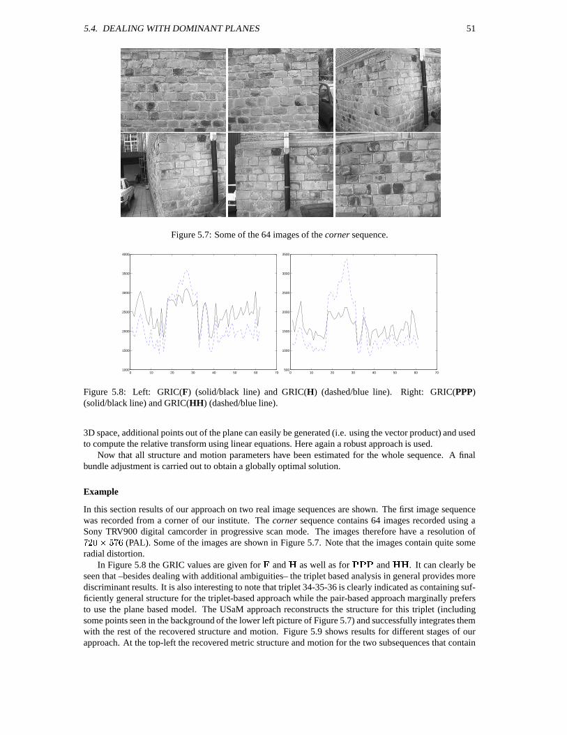
5.4. DEALING WITH DOMINANT PLANES 51
Figure 5.7: Some of the 64 images of the corner sequence.
0 10 20 30 40 50 60 701000
1500
2000
2500
3000
3500
4000
0 10 20 30 40 50 60 70500
1000
1500
2000
2500
3000
3500
Figure 5.8: Left: GRIC(F) (solid/black line) and GRIC(H) (dashed/blue line). Right: GRIC(PPP)(solid/black line) and GRIC(HH) (dashed/blue line).
3D space, additional points out of the plane can easily be generated (i.e. using the vector product) and usedto compute the relative transform using linear equations. Here again a robust approach is used.
Now that all structure and motion parameters have been estimated for the whole sequence. A finalbundle adjustment is carried out to obtain a globally optimal solution.
Example
In this section results of our approach on two real image sequences are shown. The first image sequencewas recorded from a corner of our institute. The corner sequence contains 64 images recorded using aSony TRV900 digital camcorder in progressive scan mode. The images therefore have a resolution of F(8 (PAL). Some of the images are shown in Figure 5.7. Note that the images contain quite someradial distortion.
In Figure 5.8 the GRIC values are given for
and
as well as forOO
andV
. It can clearly beseen that –besides dealing with additional ambiguities– the triplet based analysis in general provides morediscriminant results. It is also interesting to note that triplet 34-35-36 is clearly indicated as containing suf-ficiently general structure for the triplet-based approach while the pair-based approach marginally prefersto use the plane based model. The USaM approach reconstructs the structure for this triplet (includingsome points seen in the background of the lower left picture of Figure 5.7) and successfully integrates themwith the rest of the recovered structure and motion. Figure 5.9 shows results for different stages of ourapproach. At the top-left the recovered metric structure and motion for the two subsequences that contain
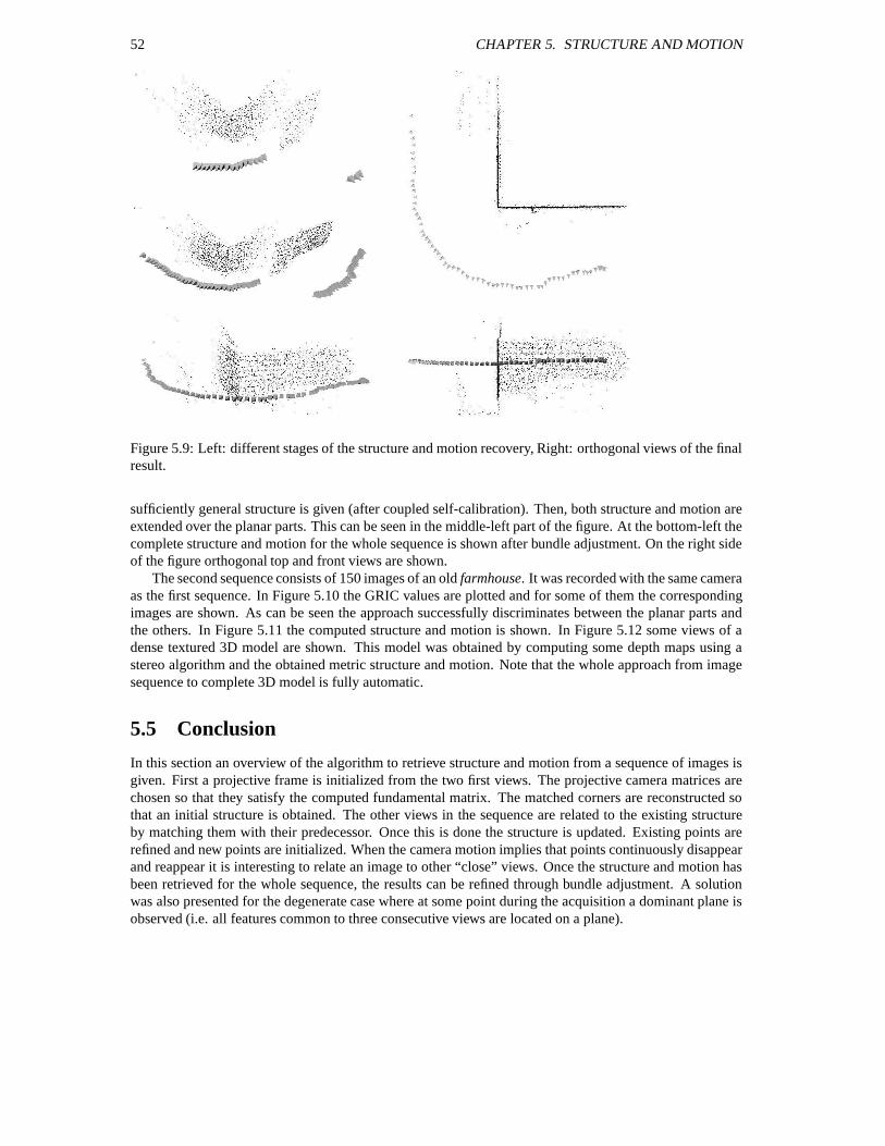
52 CHAPTER 5. STRUCTURE AND MOTION
Figure 5.9: Left: different stages of the structure and motion recovery, Right: orthogonal views of the finalresult.
sufficiently general structure is given (after coupled self-calibration). Then, both structure and motion areextended over the planar parts. This can be seen in the middle-left part of the figure. At the bottom-left thecomplete structure and motion for the whole sequence is shown after bundle adjustment. On the right sideof the figure orthogonal top and front views are shown.
The second sequence consists of 150 images of an old farmhouse. It was recorded with the same cameraas the first sequence. In Figure 5.10 the GRIC values are plotted and for some of them the correspondingimages are shown. As can be seen the approach successfully discriminates between the planar parts andthe others. In Figure 5.11 the computed structure and motion is shown. In Figure 5.12 some views of adense textured 3D model are shown. This model was obtained by computing some depth maps using astereo algorithm and the obtained metric structure and motion. Note that the whole approach from imagesequence to complete 3D model is fully automatic.
5.5 Conclusion
In this section an overview of the algorithm to retrieve structure and motion from a sequence of images isgiven. First a projective frame is initialized from the two first views. The projective camera matrices arechosen so that they satisfy the computed fundamental matrix. The matched corners are reconstructed sothat an initial structure is obtained. The other views in the sequence are related to the existing structureby matching them with their predecessor. Once this is done the structure is updated. Existing points arerefined and new points are initialized. When the camera motion implies that points continuously disappearand reappear it is interesting to relate an image to other “close” views. Once the structure and motion hasbeen retrieved for the whole sequence, the results can be refined through bundle adjustment. A solutionwas also presented for the degenerate case where at some point during the acquisition a dominant plane isobserved (i.e. all features common to three consecutive views are located on a plane).
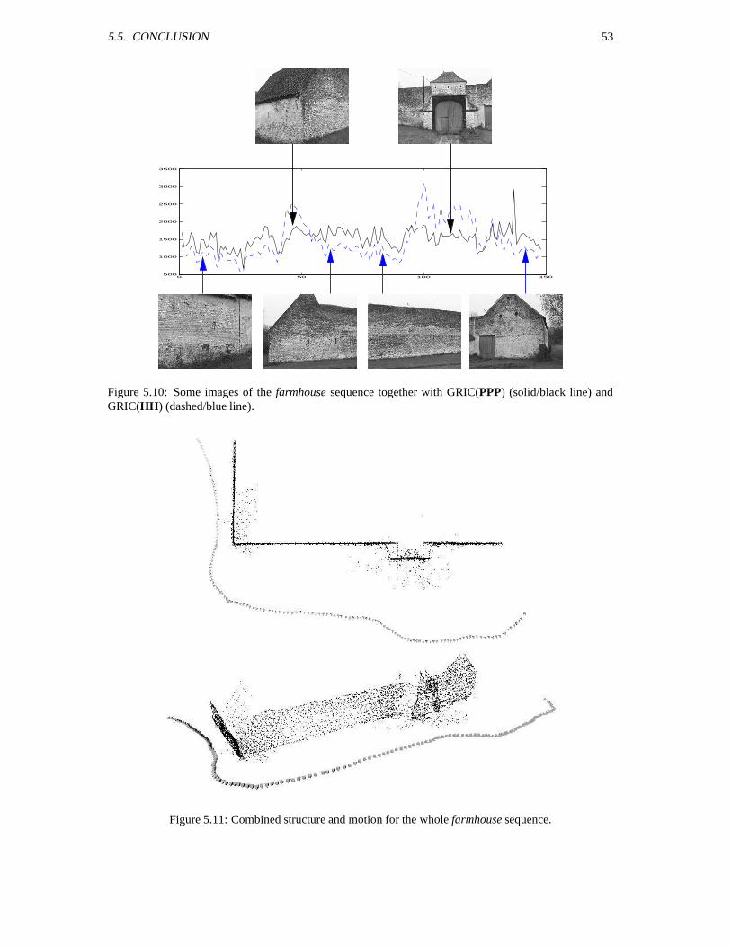
5.5. CONCLUSION 53
0 50 100 150500
1000
1500
2000
2500
3000
3500
Figure 5.10: Some images of the farmhouse sequence together with GRIC(PPP) (solid/black line) andGRIC(HH) (dashed/blue line).
Figure 5.11: Combined structure and motion for the whole farmhouse sequence.
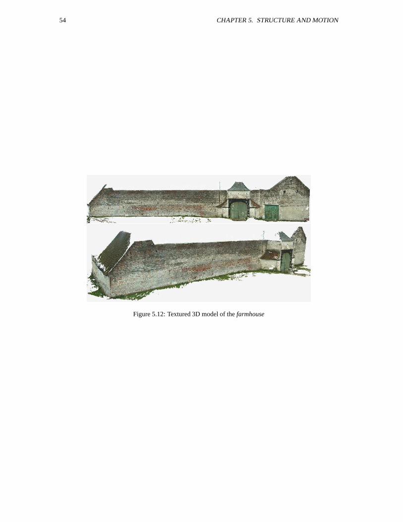
54 CHAPTER 5. STRUCTURE AND MOTION
Figure 5.12: Textured 3D model of the farmhouse
Chapter 6
Self-calibration
The reconstruction obtained as described in the previous chapters is only determined up to an arbitraryprojective transformation. This might be sufficient for some robotics or inspection applications, but cer-tainly not for visualization. Therefore we need a method to upgrade the reconstruction to a metric one (i.e.determined up to an arbitrary Euclidean transformation and a scale factor).
In general three types of constraints can be applied to achieve this: scene constraints, camera motionconstraints and constraints on the camera intrinsics. All of these have been tried separately or in con-junction. In the case of a hand-held camera and an unknown scene only the last type of constraints canbe used. Reducing the ambiguity on the reconstruction by imposing restrictions on the intrinsic cameraparameters is termed self-calibration (in the area of computer vision). In recent years many researchershave been working on this subject. Mostly self-calibration algorithms are concerned with unknown butconstant intrinsic camera parameters (see for example Faugeras et al. [32], Hartley [48], Pollefeys and VanGool [116, 118, 104], Heyden and Astrom [57] and Triggs [157]). Recently, the problem of self-calibrationin the case of varying intrinsic camera parameters was also studied (see Pollefeys et al. [115, 105, 99] andHeyden and Astrom [58, 60]).
Many researchers proposed specific self-calibration algorithms for restricted motions (i.e. combiningcamera motion constraints and camera intrinsics constraints). In several cases it turns out that simpleralgorithms can be obtained. However, the price to pay is that the ambiguity can often not be restricted tometric. Some interesting approaches were proposed by Moons et al. [89] for pure translation, Hartley [50]for pure rotations and by Armstrong et al. [2] (see also [28]) for planar motion.
Recently some methods were proposed to combine self-calibration with scene constraints. A specificcombination was proposed in [117] to resolve a case with minimal information. Bondyfalat and Boug-noux [8] proposed a method of elimination to impose the scene constraints. Liebowitz and Zisserman [79]on the other hand formulate both the scene constraints and the self-calibration constraints as constraints onthe absolute conic so that a combined approach is achieved.
Another important aspect of the self-calibration problem is the problem of critical motion sequences. Insome cases the motion of the camera is not general enough to allow for self-calibration and an ambiguityremains on the reconstruction. A first complete analysis for constant camera parameters was given bySturm [144]. Others have also worked on the subject (e.g. Pollefeys [99], Ma et al. [85] and Kahl [62]).
6.1 Calibration
In this section some existing calibration approaches are briefly discussed. These can be based on Euclideanor metric knowledge about the scene, the camera or its motion. One approach consists of first computinga projective reconstruction and then upgrading it a posteriori to a metric (or Euclidean) reconstruction byimposing some constraints. The traditional approaches however immediately go for a metric (or Euclidean)reconstruction.
55
56 CHAPTER 6. SELF-CALIBRATION
6.1.1 Scene knowledge
The knowledge of (relative) distances or angles in the scene can be used to obtain information about themetric structure. One of the easiest means to calibrate the scene at a metric level is the knowledge of therelative position of 5 or more points in general position. Assume the points
EF are the metric coordinates ofthe projectively reconstructed points
F , then the transformation
which upgrades the reconstruction fromprojective to metric can be obtained from the following equations
EF ; F or A F EF & F (6.1)
which can be rewritten as linear equations by eliminating A F . Boufama et al. [9] investigated how someEuclidean constraints could be imposed on an uncalibrated reconstruction. The constraints they dealt withare known 3D points, points on a ground plane, vertical alignment and known distances between points.Bondyfalat and Bougnoux [8] recently proposed a method in which the constraints are first processed bya geometric reasoning system so that a minimal representation of the scene is obtained. These constraintscan be incidence, parallelism and orthogonality. This minimal representation is then fed to a constrainedbundle adjustment.
The traditional approach taken by photogrammetrists [11, 41, 137, 42] consists of immediately impos-ing the position of known control points during reconstruction. These methods use bundle adjustment [12]which is a global minimization of the reprojection error. This can be expressed through the followingcriterion:
. F &
.L M WLF
N 3 F N F P P , . N 8 F N F P P , (6.2)
where is the set of indices corresponding to the points seen in view and N F P describes the projection
of a point F with camera
taking all distortions into account. Note that
F is known for control pointsand unknown for other points. It is clear that this approach results in a huge minimization problem andthat, even if the special structure of the Jacobian is taken into account (in a similar way as was explainedin Section A.2, it is computationally very expensive.
Calibration object In the case of a calibration object, the parameters of the camera are estimated usingan object with known geometry. The known calibration can then be used to obtain immediately metricreconstructions.
Many approaches exist for this type of calibration. Most of these methods consist of a two stepprocedure where a calibration is obtained first for a simplified (linear) model and then a more complexmodel, taking distortions into account, is fitted to the measurements. The difference between the methodsmainly lies in the type of calibration object that is expected (e.g. planar or not) or the complexity of thecamera model that is used. Some existing techniques are Faugeras and Toscani [27], Weng, Cohen andHerniou [170], Tsai [160, 161] (see also the implementation by Willson [173]) and Lenz and Tsai [77].
6.1.2 Camera knowledge
Knowledge about the camera can also be used to restrict the ambiguity on the reconstruction from projectiveto metric or even beyond. Different parameters of the camera can be known. Both knowledge about theextrinsic parameters (i.e. position and orientation) as the intrinsic parameters can be used for calibration.
Extrinsic parameters Knowing the relative position of the viewpoints is equivalent to knowing the rel-ative position of 3D points. Therefore the relative position of 5 viewpoints in general position sufficesto obtain a metric reconstruction. This is the principle behind the omni-rig [134] recently proposed byShashua (a similar but more restricted application was described in Pollefeys et al. [120, 119]).
It is less obvious to deal with the orientation parameters, except when the intrinsic parameters are alsoknown (see below).
6.2. SELF-CALIBRATION 57
Intrinsic parameters If the intrinsic camera parameters are known it is possible to obtain a metric recon-struction. E.g. this calibration can be obtained through off-line calibration with a calibration object. In theminimal case of 2 views and 5 points multiple solutions can exist [33], but in general a unique solution iseasily found. Traditional structure from motion algorithms assume known intrinsic parameters and obtainmetric reconstructions out of it (e.g. [80, 159, 5, 17, 140, 147]).
Intrinsic and extrinsic parameters When both intrinsic and extrinsic camera parameters are known, thefull camera projection matrix is determined. In this case a Euclidean reconstruction is obtained immediatelyby back-projecting the points.
In the case of known relative position and orientation of the cameras, the first view can be aligned withthe world frame without loss of generality. If only the (relative) orientation and the intrinsic parametersare known, the first T part of the camera projection matrices is known and it is still possible to linearlyobtain the transformation which upgrades the projective reconstruction to metric.
6.2 Self-calibration
In this section some importants concepts for self-calibration are introduced. These are then used to brieflydescribe some of the existing self-calibration methods.
6.2.1 A counting argument
To restrict the projective ambiguity (15 degrees of freedom) to a metric one (3 degrees of freedom forrotation, 3 for translation and 1 for scale), at least 8 constraints are needed. This thus determines theminimum length of a sequence from which self-calibration can be obtained, depending on the type ofconstraints which are available for each view. Knowing an intrinsic camera parameter for , views gives ,constraints, fixing one yields only , constraints.
,C N %, , P . N , P N +3 P
Of course this counting argument is only valid if all the constraints are independent. In this context criticalmotion sequences are of special importance (see Section 6.2.5).
Therefore the absence of skew (1 constraint per view) should in general be enough to allow self-calibration on a sequence of 8 or more images (this was shown in [114, 60, 99]). If in addition the aspectratio is known (e.g. & ) then 4 views should be sufficient. When the principal point is known as wella pair of images is sufficient.
6.2.2 Geometric interpretation of constraints
In this section a geometric interpretation of a camera projection matrix is given. It is seen that constraintson the internal camera parameters can easily be given a geometric interpretation in space.
A camera projection plane defines a set of three planes. The first one is parallel to the image and goesthrough the center of projection. This plane can be obtained by back-projecting the line at infinity of theimage (i.e. 1 (F( 5 S ). The two others respectively correspond to the back-projection of the image 3 - and8 -axis (i.e. 1 ( ( 5 S and 1 (F( 5 S resp.). A line can be back-projected through equation (3.9):
; S ; "- S " ! S (6.3)
Let us look at the relative orientation of these planes. Therefore the rotation and translation can be left outwithout loss of generality (i.e. a camera centered representation is used). Let us then define the vectors , and as the first three coefficients of these planes. This then yields the following three vectors:
& (
&
&
((
(6.4)
58 CHAPTER 6. SELF-CALIBRATION
The vectors coinciding with the direction of the 3 and the 8 axis can be obtained by intersections of theseplanes:
& &
((
and
& &
(
(6.5)
The following dot products can now be taken:
& & and & (6.6)
Equation (6.6) proves that the constraint for rectangular pixels (i.e. & ( ), and zero coordinates for theprincipal point (i.e. & ( and & ( ) can all be expressed in terms of orthogonality between vectorsin space. Note further that it is possible to pre-warp the image so that a known skew1 or known principalpoint parameters coincide with zero. Similarly a known focal length or aspect ratio can be scaled to one.
The AC is also possible to give a geometric interpretation to a known focal length or aspect ratio. Puta plane parallel with the image at distance
from the center of projection (i.e. 3 &
in camera centeredcoordinates). In this case a horizontal motion in the image of pixels will move the intersection point ofthe line of sight over a distance
. In other words a known focal length is equivalent to knowing that the
length of two (typically orthogonal) vectors are equal. If the aspect ratio is defined as the ratio betweenthe horizontal and vertical sides of a pixel (which makes it independent of ), a similar interpretation ispossible.
6.2.3 The image of the absolute conic
One of the most important concepts for self-calibration is the Absolute Conic (AC) and its projection inthe images (IAC) 2. Since it is invariant under Euclidean transformations (see Section 2.2.3), its relativeposition to a moving camera is constant. For constant intrinsic camera parameters its image will thereforealso be constant. This is similar to someone who has the impression that the moon is following him whendriving on a straight road. Note that the AC is more general, because it is not only invariant to translationsbut also to arbitrary rotations.
It can be seen as a calibration object which is naturally present in all the scenes. Once the AC islocalized, it can be used to upgrade the reconstruction to metric. It is, however, not always so simple tofind the AC in the reconstructed space. In some cases it is not possible to make the difference between thetrue AC and other candidates. This problem will be discussed in the Section 6.2.5.
In practice the simplest way to represent the AC is through the Dual Absolute Quadric (DAQ). In thiscase both the AC and its supporting plane, the plane at infinity, are expressed through one geometric entity.The relationship between the AC and the IAC is easily obtained using the projection equation for the DAQ:
9 7 ; * 7 S (6.7)
with 9 7 representing the dual of the IAC,*67
the DAQ and
the projection matrix for view . Figure 6.1illustrates these concepts. For a Euclidean representation of the world the camera projection matricescan be factorized as:
& ! " S 1 \ - 5 (with!
an upper triangular matrix containing the intrinsiccamera parameters,
" Srepresenting the orientation and
the position) and the DAQ can be written as*57 & N ( P . Substituting this in Equation (6.7), one obtains:
9 7 ; ! ! S (6.8)
This equation is very useful because it immediately relates the intrinsic camera parameters to the DIAC.In the case of a projective representation of the world the DAQ will not be at its standard position, but
will have the following form:*67 & *57 S with
being the transformation from the metric to the
projective representation. But, since the images were obtained in a Euclidean world, the images 9 7 stillsatisfy Equation (6.8). If
*67is retrieved, it is possible to upgrade the geometry from projective to metric.
1In this case the skew should be given as an angle in the image plane. If the aspect ratio is also known, this corresponds to anangle in the retinal plane (e.g. CCD-array).
2See Section 2.2.3 for details.
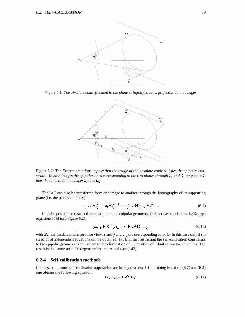
6.2. SELF-CALIBRATION 59
i
C
Cωi
Π oo
Ω
j
jω
Figure 6.1: The absolute conic (located in the plane at infinity) and its projection in the images
Ci
C
l
l’
l’
ii
1
2
Π
Ω
e
i
j
j
j
je
L’
oo
l
L
ω
ω
Figure 6.2: The Kruppa equations impose that the image of the absolute conic satisfies the epipolar con-straint. In both images the epipolar lines corresponding to the two planes through
and
tangent to
*must be tangent to the images 9 and 9 .
The IAC can also be transferred from one image to another through the homography of its supportingplane (i.e. the plane at infinity):
9 ; # U S 9 #L UXW or 9 7 ; #L 9 7 # S (6.9)
It is also possible to restrict this constraint to the epipolar geometry. In this case one obtains the Kruppaequations [75] (see Figure 6.2):
1 L 5 S !V! S 1 L 5 ; !V! S S (6.10)
with L
the fundamental matrix for views and and L the corresponding epipole. In this case only 2 (instead of 5) independent equations can be obtained [176]. In fact restricting the self-calibration constraintsto the epipolar geometry is equivalent to the elimination of the position of infinity from the equations. Theresult is that some artificial degeneracies are created (see [142]).
6.2.4 Self-calibration methods
In this section some self-calibration approaches are briefly discussed. Combining Equation (6.7) and (6.8)one obtains the following equation: ! ! S ; * 7 S (6.11)
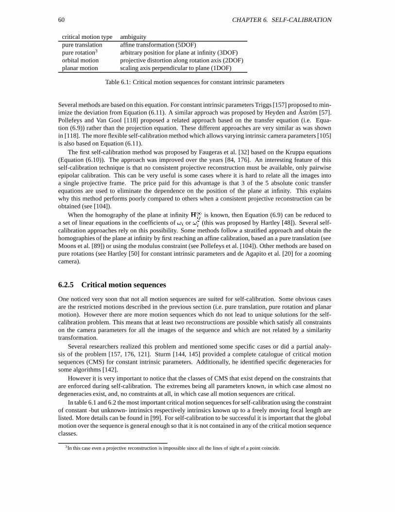
60 CHAPTER 6. SELF-CALIBRATION
critical motion type ambiguitypure translation affine transformation (5DOF)pure rotation3 arbitrary position for plane at infinity (3DOF)orbital motion projective distortion along rotation axis (2DOF)planar motion scaling axis perpendicular to plane (1DOF)
Table 6.1: Critical motion sequences for constant intrinsic parameters
Several methods are based on this equation. For constant intrinsic parameters Triggs [157] proposed to min-imize the deviation from Equation (6.11). A similar approach was proposed by Heyden and Astrom [57].Pollefeys and Van Gool [118] proposed a related approach based on the transfer equation (i.e. Equa-tion (6.9)) rather than the projection equation. These different approaches are very similar as was shownin [118]. The more flexible self-calibration method which allows varying intrinsic camera parameters [105]is also based on Equation (6.11).
The first self-calibration method was proposed by Faugeras et al. [32] based on the Kruppa equations(Equation (6.10)). The approach was improved over the years [84, 176]. An interesting feature of thisself-calibration technique is that no consistent projective reconstruction must be available, only pairwiseepipolar calibration. This can be very useful is some cases where it is hard to relate all the images intoa single projective frame. The price paid for this advantage is that 3 of the 5 absolute conic transferequations are used to eliminate the dependence on the position of the plane at infinity. This explainswhy this method performs poorly compared to others when a consistent projective reconstruction can beobtained (see [104]).
When the homography of the plane at infinity #L
is known, then Equation (6.9) can be reduced toa set of linear equations in the coefficients of 9 or 9 7 (this was proposed by Hartley [48]). Several self-calibration approaches rely on this possibility. Some methods follow a stratified approach and obtain thehomographies of the plane at infinity by first reaching an affine calibration, based an a pure translation (seeMoons et al. [89]) or using the modulus constraint (see Pollefeys et al. [104]). Other methods are based onpure rotations (see Hartley [50] for constant intrinsic parameters and de Agapito et al. [20] for a zoomingcamera).
6.2.5 Critical motion sequences
One noticed very soon that not all motion sequences are suited for self-calibration. Some obvious casesare the restricted motions described in the previous section (i.e. pure translation, pure rotation and planarmotion). However there are more motion sequences which do not lead to unique solutions for the self-calibration problem. This means that at least two reconstructions are possible which satisfy all constraintson the camera parameters for all the images of the sequence and which are not related by a similaritytransformation.
Several researchers realized this problem and mentioned some specific cases or did a partial analy-sis of the problem [157, 176, 121]. Sturm [144, 145] provided a complete catalogue of critical motionsequences (CMS) for constant intrinsic parameters. Additionally, he identified specific degeneracies forsome algorithms [142].
However it is very important to notice that the classes of CMS that exist depend on the constraints thatare enforced during self-calibration. The extremes being all parameters known, in which case almost nodegeneracies exist, and, no constraints at all, in which case all motion sequences are critical.
In table 6.1 and 6.2 the most important critical motion sequences for self-calibration using the constraintof constant -but unknown- intrinsics respectively intrinsics known up to a freely moving focal length arelisted. More details can be found in [99]. For self-calibration to be successful it is important that the globalmotion over the sequence is general enough so that it is not contained in any of the critical motion sequenceclasses.
3In this case even a projective reconstruction is impossible since all the lines of sight of a point coincide.
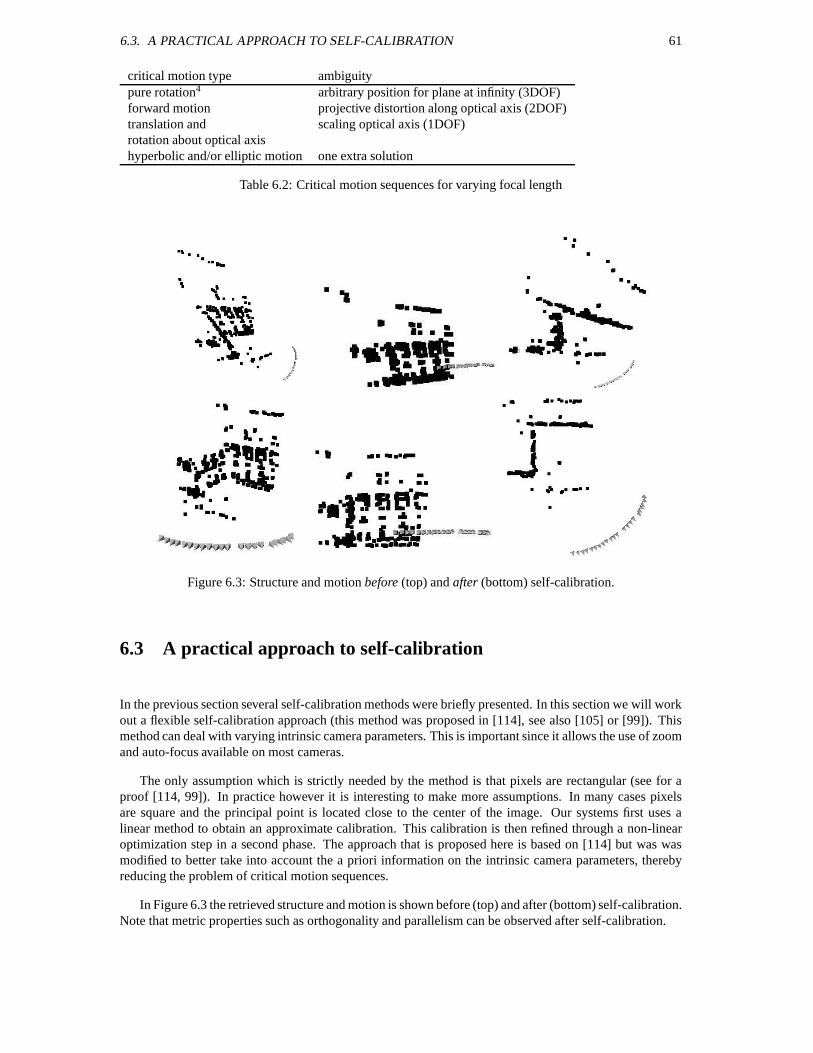
6.3. A PRACTICAL APPROACH TO SELF-CALIBRATION 61
critical motion type ambiguitypure rotation4 arbitrary position for plane at infinity (3DOF)forward motion projective distortion along optical axis (2DOF)translation and scaling optical axis (1DOF)rotation about optical axishyperbolic and/or elliptic motion one extra solution
Table 6.2: Critical motion sequences for varying focal length
Figure 6.3: Structure and motion before (top) and after (bottom) self-calibration.
6.3 A practical approach to self-calibration
In the previous section several self-calibration methods were briefly presented. In this section we will workout a flexible self-calibration approach (this method was proposed in [114], see also [105] or [99]). Thismethod can deal with varying intrinsic camera parameters. This is important since it allows the use of zoomand auto-focus available on most cameras.
The only assumption which is strictly needed by the method is that pixels are rectangular (see for aproof [114, 99]). In practice however it is interesting to make more assumptions. In many cases pixelsare square and the principal point is located close to the center of the image. Our systems first uses alinear method to obtain an approximate calibration. This calibration is then refined through a non-linearoptimization step in a second phase. The approach that is proposed here is based on [114] but was wasmodified to better take into account the a priori information on the intrinsic camera parameters, therebyreducing the problem of critical motion sequences.
In Figure 6.3 the retrieved structure and motion is shown before (top) and after (bottom) self-calibration.Note that metric properties such as orthogonality and parallelism can be observed after self-calibration.
62 CHAPTER 6. SELF-CALIBRATION
6.3.1 linear self-calibration
The first step consists of normalizing the projection matrices. The following normalization is proposed:
& ! UZW with! &
. ( , . ,
(6.12)
where and
are the width, resp. height of the image. After the normalization the focal length should beof the order of unity and the principal point should be close to the origin. The above normalization wouldscale a focal length of a 60mm lens to 1 and thus focal lengths in the range of 20mm to 180mm wouldend up in the range 1 5 . The aspect ratio is typically also around 1 and the skew can be assumed 0 forall practical purposes. Making these a priori knowledge more explicit and estimating reasonable standarddeviations one could for example get , (1( , ( and &D( . It is nowinteresting to investigate the impact of this knowledge on 9 7 :
9 7 ; !V! S &
, . , . , 8. . , ,/. ,
( ( ( ( ( ( ( (
(6.13)
and 9 7, , 9 7W W 1( . The constraints on the left-hand side of Equation (6.7) should also be verified on
the right-hand side (up to scale). The uncertainty can be take into account by weighting the equations.W W *57 W S *57 S & (W , *57 , S *57 S & (W, W
*57 W S , *57 , S & (W W W * 7 , S & (W W W *57 S & (W W , * 7 S & (
(6.14)
with the th row of
and a scale factor that is initially set to 1 and later on to *57 S with*57the result of the previous iteration. Since
* 7is a symmetric matrix it is parametrized through
10 coefficients. An estimate of the dual absolute quadric* 7
can be obtained by solving the above set ofequations for all views through linear least-squares. The rank-3 constraint should be imposed by forcing thesmallest singular value to zero. This scheme can be iterated until the factors converge, but in practice thisis often not necessary. Experimental validation has shown that this approach yields much better results thanthe original approach described in [114, 105]. This is mostly due to the fact that constraining all parameters(even with a small weight) allows to avoid most of the problems due to critical motion sequences [144, 63](especially the specific additional case for the linear algorithm [99]).
coupled self-calibration
In some cases different (sub)sequences have been recorded with the same camera and the same settings. Inthis case it is possible to combine the equations derived above into a larger system of equations. This canfor example be used to solve the problem of a dominant plane separating a sequence in two subsequences(see Section 5.4).
When choosing &K1 \ 5 for one of the projection matrices it can be seen from Equation (6.11) that 7
can be written as: 7 & !V! S S (6.15)
Now the set of equations (6.14) can thus be written as:
(6.16)
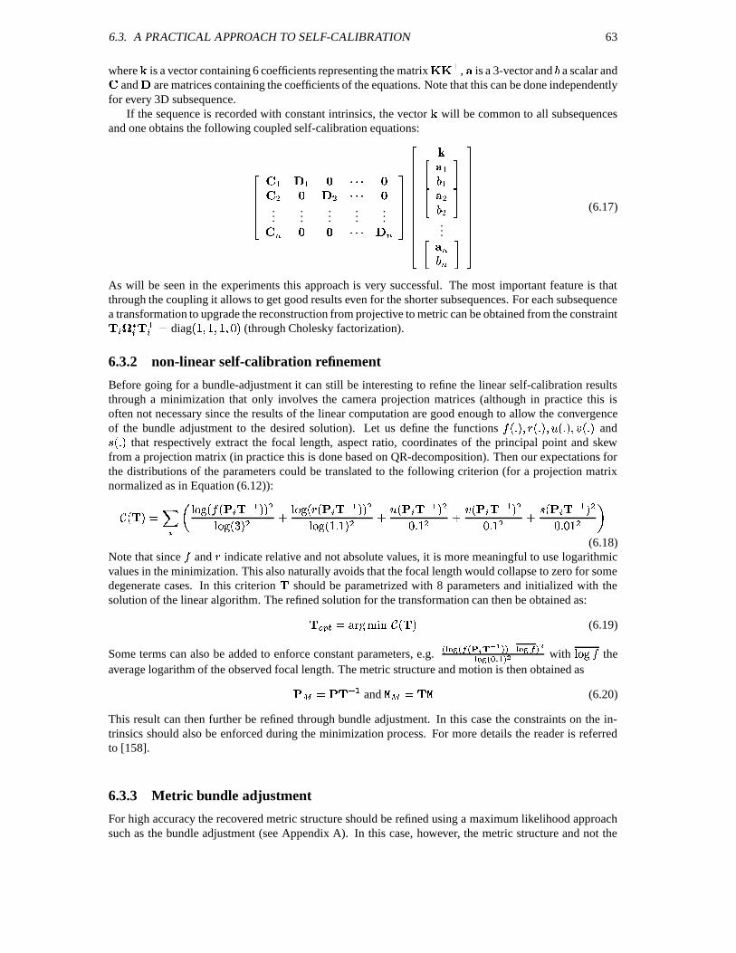
6.3. A PRACTICAL APPROACH TO SELF-CALIBRATION 63
where
is a vector containing 6 coefficients representing the matrix!V! S
,
is a 3-vector and
a scalar and
and
are matrices containing the coefficients of the equations. Note that this can be done independentlyfor every 3D subsequence.
If the sequence is recorded with constant intrinsics, the vector
will be common to all subsequencesand one obtains the following coupled self-calibration equations:
W W
,
,
......
......
...
.
.
W W ,, ... ..
(6.17)
As will be seen in the experiments this approach is very successful. The most important feature is thatthrough the coupling it allows to get good results even for the shorter subsequences. For each subsequencea transformation to upgrade the reconstruction from projective to metric can be obtained from the constraint 7 S & diag
N ( P (through Cholesky factorization).
6.3.2 non-linear self-calibration refinement
Before going for a bundle-adjustment it can still be interesting to refine the linear self-calibration resultsthrough a minimization that only involves the camera projection matrices (although in practice this isoften not necessary since the results of the linear computation are good enough to allow the convergenceof the bundle adjustment to the desired solution). Let us define the functions N P N P N P N P and N P that respectively extract the focal length, aspect ratio, coordinates of the principal point and skewfrom a projection matrix (in practice this is done based on QR-decomposition). Then our expectations forthe distributions of the parameters could be translated to the following criterion (for a projection matrixnormalized as in Equation (6.12)):
N P & L N N UZW P P , N P , .
N N UZW P P , N P , . N UZW P ,( , .
N UZW P ,( , . N UZW P ,
( ( ,
(6.18)Note that since and
indicate relative and not absolute values, it is more meaningful to use logarithmic
values in the minimization. This also naturally avoids that the focal length would collapse to zero for somedegenerate cases. In this criterion
should be parametrized with 8 parameters and initialized with the
solution of the linear algorithm. The refined solution for the transformation can then be obtained as:
& N P
(6.19)
Some terms can also be added to enforce constant parameters, e.g.
U W with
theaverage logarithm of the observed focal length. The metric structure and motion is then obtained as
& UZW and & (6.20)
This result can then further be refined through bundle adjustment. In this case the constraints on the in-trinsics should also be enforced during the minimization process. For more details the reader is referredto [158].
6.3.3 Metric bundle adjustment
For high accuracy the recovered metric structure should be refined using a maximum likelihood approachsuch as the bundle adjustment (see Appendix A). In this case, however, the metric structure and not the
64 CHAPTER 6. SELF-CALIBRATION
projective structure is retrieved. This means that the camera projection matrices should be parametrizedusing intrinsic and extrinsic parameters (and not in homogeneous form as in the projective case). If oneassumes that the error is only due to mislocalization of the image features and that this error is uniformand normally distributed5, the bundle adjustment corresponds to a maximum likelihood estimator. For thisto be satisfied the camera model should be general enoguh so that no systematic errors remain in the data(e.g. due to lens distortion). In these circumstances the maximum likelihood estimation corresponds tothe solution of a least-squares problem. In this case a criterion of the type of equation (6.2) should beminimized:
N F ! " P & .L M WLF
N 3 F W F FP , . N 8 F
, F
FP , (6.21)
where is the set of indices corresponding to the points seen in view and S W S ,
S S &! 1 " S -" S 5 . This criterion should be extended with terms that reflect the (un)certainty on the intrinsic
camera parameters. This would yield a criterion of the following form:
E N F ! " P & K . M W K F N 3 F P , . N 8 F P , . K . M W K > M W A N ! P , (6.22)
with A a regularization factor and N ! P representing the constraints on the intrinsic camera parameters,e.g. W &
(known aspect ratio), ,
&
(known principal point) or (constant focal
length). The values of the factors A depend on how strongly the constraints should be enforced.
6.4 Conclusion
In this chapter we discussed how to restrict the projective ambiguity of the reconstruction to metric (i.e.Euclidean up to scale). After a brief discussion of traditional calibration approaches, we focussed on theproblem of self-calibration. The general concepts were introduced and the most important methods brieflypresented. Then a flexible self-calibration approach that can deal with focusing/zooming cameras wasworked out in detail.
5This is a realistic assumption since outliers should have been removed at this stage of the processing.
Chapter 7
Dense depth estimation
With the camera calibration given for all viewpoints of the sequence, we can proceed with methods de-veloped for calibrated structure from motion algorithms. The feature tracking algorithm already deliversa sparse surface model based on distinct feature points. This however is not sufficient to reconstruct ge-ometrically correct and visually pleasing surface models. This task is accomplished by a dense disparitymatching that estimates correspondences from the grey level images directly by exploiting additional geo-metrical constraints.
This chapter is organized as follows. In a first section rectification is discussed. This makes it possibleto use standard stereo matching techniques on image pairs. Stereo matching is discussed in a secondsection. Finally a multi-view approach that allows to integrate the results obtained from several pairs ispresented.
7.1 Image pair rectification
The stereo matching problem can be solved much more efficiently if images are rectified. This step consistsof transforming the images so that the epipolar lines are aligned horizontally. In this case stereo match-ing algorithms can easily take advantage of the epipolar constraint and reduce the search space to onedimension (i.e. corresponding rows of the rectified images).
The traditional rectification scheme consists of transforming the image planes so that the correspondingspace planes are coinciding [4]. There exist many variants of this traditional approach (e.g. [4, 29, 96, 179]),it was even implemented in hardware [15]. This approach fails when the epipoles are located in the imagessince this would have to results in infinitely large images. Even when this is not the case the image can stillbecome very large (i.e. if the epipole is close to the image).
Roy et al. [128] proposed a method to avoid this problem, but their approach is relatively complex andshows some problems. Recently Pollefeys et al. [106] proposed a simple method which guarantees minimalimage size and works for all possible configuration. This method will be presented in detail further on, butfirst the standard planar rectification is briefly discussed.
7.1.1 Planar rectification
The standard rectification approach is relatively simple. It consists of selecting a plane parallel with thebaseline. The two image are then reprojected into this plane. This is illustrated in Figure 7.1. These newimages satisfy the standard stereo setup. The different methods for rectification mainly differ in how theremaining degrees of freedom are chosen. In the calibrated case one can choose the distance from the planeto the baseline so that no pixels are compressed during the warping from the images to the rectified imagesand the normal on the plane can be chosen in the middle of the two epipolar planes containing the opticalaxes. In the uncalibrated case the choice is less obvious. Several approaches were proposed (e.g. [29, 179]).
65
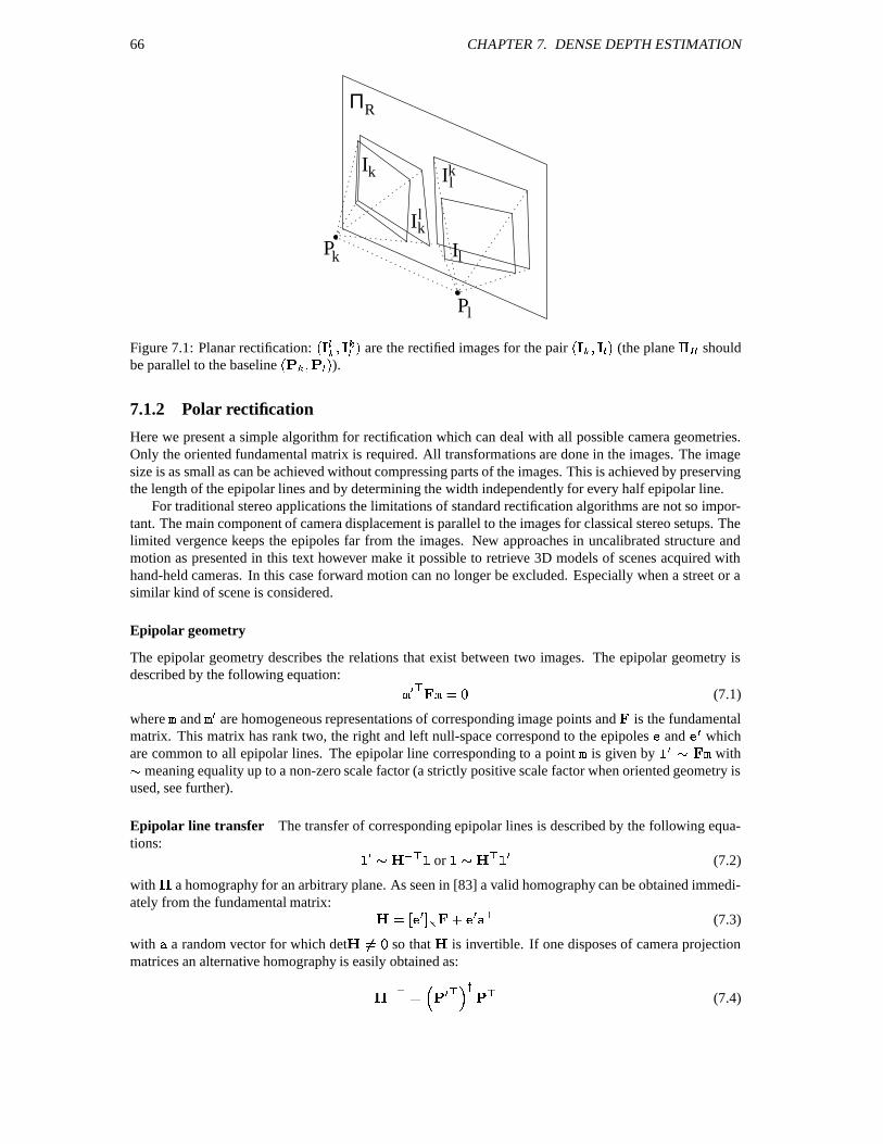
66 CHAPTER 7. DENSE DEPTH ESTIMATION
I
I
RΠ
l
k
P
I
Il
kl
lk
k
P
Figure 7.1: Planar rectification:N \ F \ F P are the rectified images for the pair
N \ \ F P (the plane shouldbe parallel to the baseline
N F P ).7.1.2 Polar rectification
Here we present a simple algorithm for rectification which can deal with all possible camera geometries.Only the oriented fundamental matrix is required. All transformations are done in the images. The imagesize is as small as can be achieved without compressing parts of the images. This is achieved by preservingthe length of the epipolar lines and by determining the width independently for every half epipolar line.
For traditional stereo applications the limitations of standard rectification algorithms are not so impor-tant. The main component of camera displacement is parallel to the images for classical stereo setups. Thelimited vergence keeps the epipoles far from the images. New approaches in uncalibrated structure andmotion as presented in this text however make it possible to retrieve 3D models of scenes acquired withhand-held cameras. In this case forward motion can no longer be excluded. Especially when a street or asimilar kind of scene is considered.
Epipolar geometry
The epipolar geometry describes the relations that exist between two images. The epipolar geometry isdescribed by the following equation: E S & ( (7.1)
where and E are homogeneous representations of corresponding image points and
is the fundamentalmatrix. This matrix has rank two, the right and left null-space correspond to the epipoles and E whichare common to all epipolar lines. The epipolar line corresponding to a point is given by
E ; with; meaning equality up to a non-zero scale factor (a strictly positive scale factor when oriented geometry isused, see further).
Epipolar line transfer The transfer of corresponding epipolar lines is described by the following equa-tions: E ; UZS or
; S E (7.2)
with
a homography for an arbitrary plane. As seen in [83] a valid homography can be obtained immedi-ately from the fundamental matrix: &21 E 5 . E S (7.3)
with a random vector for which det B&>( so that
is invertible. If one disposes of camera projection
matrices an alternative homography is easily obtained as:
U S & E S ] S (7.4)
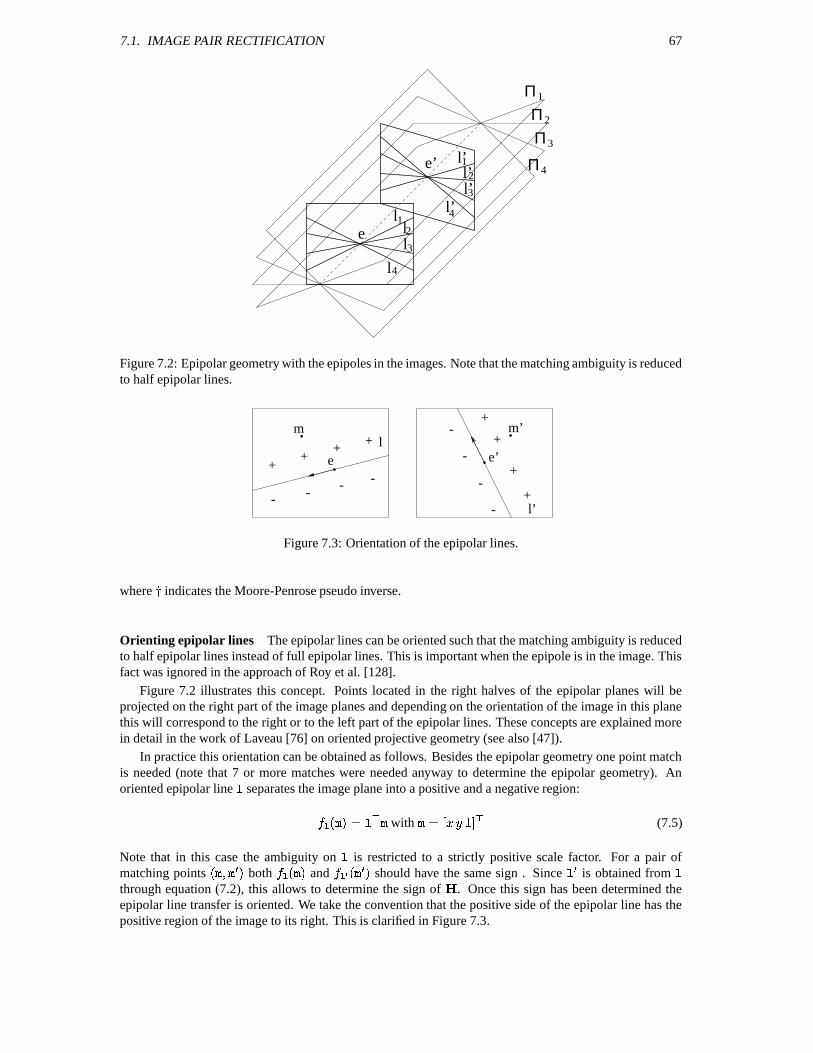
7.1. IMAGE PAIR RECTIFICATION 67
l4
l’4
3
1l2l
3
Π3
4Π
2
l’
l
1ΠΠ
1e’2l’
l’
e
Figure 7.2: Epipolar geometry with the epipoles in the images. Note that the matching ambiguity is reducedto half epipolar lines.
+
---
m’
l’
le
+
+
+
+e’
++
m
-
-
-
-
+
-
Figure 7.3: Orientation of the epipolar lines.
where indicates the Moore-Penrose pseudo inverse.
Orienting epipolar lines The epipolar lines can be oriented such that the matching ambiguity is reducedto half epipolar lines instead of full epipolar lines. This is important when the epipole is in the image. Thisfact was ignored in the approach of Roy et al. [128].
Figure 7.2 illustrates this concept. Points located in the right halves of the epipolar planes will beprojected on the right part of the image planes and depending on the orientation of the image in this planethis will correspond to the right or to the left part of the epipolar lines. These concepts are explained morein detail in the work of Laveau [76] on oriented projective geometry (see also [47]).
In practice this orientation can be obtained as follows. Besides the epipolar geometry one point matchis needed (note that 7 or more matches were needed anyway to determine the epipolar geometry). Anoriented epipolar line
separates the image plane into a positive and a negative region:
N P & S with &21 3 8 5 S (7.5)
Note that in this case the ambiguity on
is restricted to a strictly positive scale factor. For a pair ofmatching points
N E P both N P and N E P should have the same sign . Since E is obtained from
through equation (7.2), this allows to determine the sign of
. Once this sign has been determined the
epipolar line transfer is oriented. We take the convention that the positive side of the epipolar line has thepositive region of the image to its right. This is clarified in Figure 7.3.
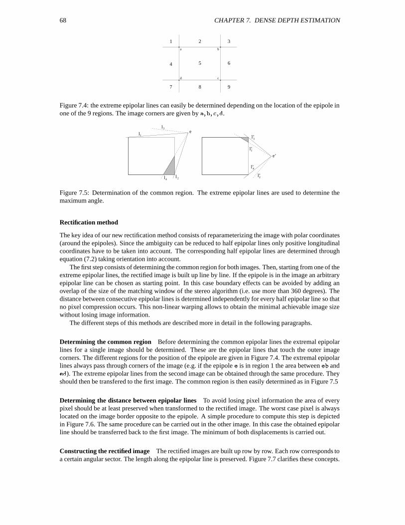
68 CHAPTER 7. DENSE DEPTH ESTIMATION
98
64
3
c
ba
1 2
5
7
d
Figure 7.4: the extreme epipolar lines can easily be determined depending on the location of the epipole inone of the 9 regions. The image corners are given by .
l’
4
3
3l
l l’
1
2l
l
1
2
l’
l’
4
e’
e
Figure 7.5: Determination of the common region. The extreme epipolar lines are used to determine themaximum angle.
Rectification method
The key idea of our new rectification method consists of reparameterizing the image with polar coordinates(around the epipoles). Since the ambiguity can be reduced to half epipolar lines only positive longitudinalcoordinates have to be taken into account. The corresponding half epipolar lines are determined throughequation (7.2) taking orientation into account.
The first step consists of determining the common region for both images. Then, starting from one of theextreme epipolar lines, the rectified image is built up line by line. If the epipole is in the image an arbitraryepipolar line can be chosen as starting point. In this case boundary effects can be avoided by adding anoverlap of the size of the matching window of the stereo algorithm (i.e. use more than 360 degrees). Thedistance between consecutive epipolar lines is determined independently for every half epipolar line so thatno pixel compression occurs. This non-linear warping allows to obtain the minimal achievable image sizewithout losing image information.
The different steps of this methods are described more in detail in the following paragraphs.
Determining the common region Before determining the common epipolar lines the extremal epipolarlines for a single image should be determined. These are the epipolar lines that touch the outer imagecorners. The different regions for the position of the epipole are given in Figure 7.4. The extremal epipolarlines always pass through corners of the image (e.g. if the epipole is in region 1 the area between and ). The extreme epipolar lines from the second image can be obtained through the same procedure. Theyshould then be transfered to the first image. The common region is then easily determined as in Figure 7.5
Determining the distance between epipolar lines To avoid losing pixel information the area of everypixel should be at least preserved when transformed to the rectified image. The worst case pixel is alwayslocated on the image border opposite to the epipole. A simple procedure to compute this step is depictedin Figure 7.6. The same procedure can be carried out in the other image. In this case the obtained epipolarline should be transferred back to the first image. The minimum of both displacements is carried out.
Constructing the rectified image The rectified images are built up row by row. Each row corresponds toa certain angular sector. The length along the epipolar line is preserved. Figure 7.7 clarifies these concepts.
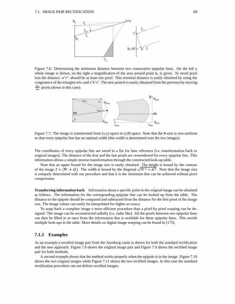
7.1. IMAGE PAIR RECTIFICATION 69
l
li-1
e=c
l
l
l1
n
l c’
i
i
b =b’i
i-1
a
a’
bi
Figure 7.6: Determining the minimum distance between two consecutive epipolar lines. On the left awhole image is shown, on the right a magnification of the area around point
is given. To avoid pixel
loss the distance $E E should be at least one pixel. This minimal distance is easily obtained by using the
congruence of the triangles and $E E E . The new point
is easily obtained from the previous by moving
pixels (down in this case).
x
y r
θ
r
rmax
θmax
min
θmin
θmaxrmax
θ
i
minminr
∆θi ∆θ
Figure 7.7: The image is transformed from (x,y)-space to (r, )-space. Note that the -axis is non-uniformso that every epipolar line has an optimal width (this width is determined over the two images).
The coordinates of every epipolar line are saved in a list for later reference (i.e. transformation back tooriginal images). The distance of the first and the last pixels are remembered for every epipolar line. Thisinformation allows a simple inverse transformation through the constructed look-up table.
Note that an upper bound for the image size is easily obtained. The height is bound by the contourof the image T N % . P . The width is bound by the diagonal % , . , . Note that the image sizeis uniquely determined with our procedure and that it is the minimum that can be achieved without pixelcompression.
Transferring information back Information about a specific point in the original image can be obtainedas follows. The information for the corresponding epipolar line can be looked up from the table. Thedistance to the epipole should be computed and subtracted from the distance for the first pixel of the imagerow. The image values can easily be interpolated for higher accuracy.
To warp back a complete image a more efficient procedure than a pixel-by-pixel warping can be de-signed. The image can be reconstructed radially (i.e. radar like). All the pixels between two epipolar linescan then be filled in at once from the information that is available for these epipolar lines. This avoidsmultiple look-ups in the table. More details on digital image warping can be found in [175].
7.1.3 Examples
As an example a rectified image pair from the Arenberg castle is shown for both the standard rectificationand the new approach. Figure 7.8 shows the original image pair and Figure 7.9 shows the rectified imagepair for both methods.
A second example shows that the method works properly when the epipole is in the image. Figure 7.10shows the two original images while Figure 7.11 shows the two rectified images. In this case the standardrectification procedure can not deliver rectified images.
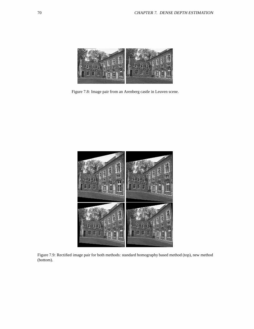
70 CHAPTER 7. DENSE DEPTH ESTIMATION
Figure 7.8: Image pair from an Arenberg castle in Leuven scene.
Figure 7.9: Rectified image pair for both methods: standard homography based method (top), new method(bottom).
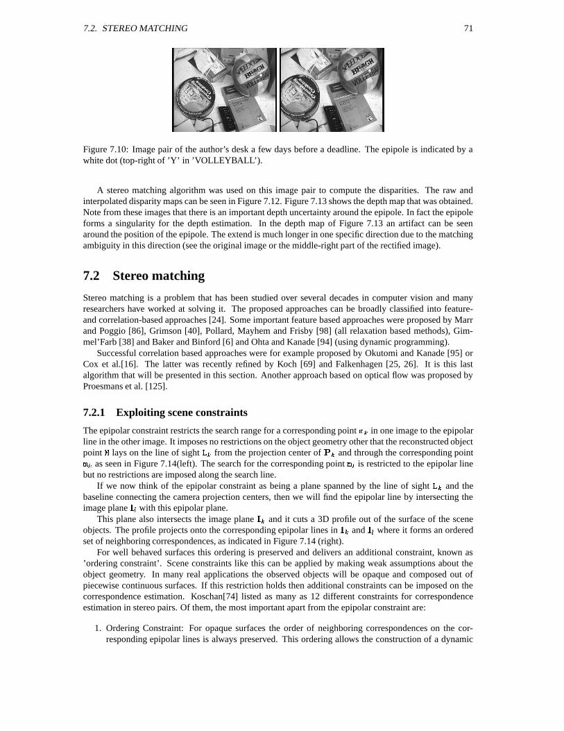
7.2. STEREO MATCHING 71
Figure 7.10: Image pair of the author’s desk a few days before a deadline. The epipole is indicated by awhite dot (top-right of ’Y’ in ’VOLLEYBALL’).
A stereo matching algorithm was used on this image pair to compute the disparities. The raw andinterpolated disparity maps can be seen in Figure 7.12. Figure 7.13 shows the depth map that was obtained.Note from these images that there is an important depth uncertainty around the epipole. In fact the epipoleforms a singularity for the depth estimation. In the depth map of Figure 7.13 an artifact can be seenaround the position of the epipole. The extend is much longer in one specific direction due to the matchingambiguity in this direction (see the original image or the middle-right part of the rectified image).
7.2 Stereo matching
Stereo matching is a problem that has been studied over several decades in computer vision and manyresearchers have worked at solving it. The proposed approaches can be broadly classified into feature-and correlation-based approaches [24]. Some important feature based approaches were proposed by Marrand Poggio [86], Grimson [40], Pollard, Mayhem and Frisby [98] (all relaxation based methods), Gim-mel’Farb [38] and Baker and Binford [6] and Ohta and Kanade [94] (using dynamic programming).
Successful correlation based approaches were for example proposed by Okutomi and Kanade [95] orCox et al.[16]. The latter was recently refined by Koch [69] and Falkenhagen [25, 26]. It is this lastalgorithm that will be presented in this section. Another approach based on optical flow was proposed byProesmans et al. [125].
7.2.1 Exploiting scene constraints
The epipolar constraint restricts the search range for a corresponding point in one image to the epipolarline in the other image. It imposes no restrictions on the object geometry other that the reconstructed objectpoint
lays on the line of sight from the projection center of
and through the corresponding point as seen in Figure 7.14(left). The search for the corresponding point F is restricted to the epipolar linebut no restrictions are imposed along the search line.
If we now think of the epipolar constraint as being a plane spanned by the line of sight and thebaseline connecting the camera projection centers, then we will find the epipolar line by intersecting theimage plane \ F with this epipolar plane.
This plane also intersects the image plane \ and it cuts a 3D profile out of the surface of the sceneobjects. The profile projects onto the corresponding epipolar lines in \ and \ F where it forms an orderedset of neighboring correspondences, as indicated in Figure 7.14 (right).
For well behaved surfaces this ordering is preserved and delivers an additional constraint, known as’ordering constraint’. Scene constraints like this can be applied by making weak assumptions about theobject geometry. In many real applications the observed objects will be opaque and composed out ofpiecewise continuous surfaces. If this restriction holds then additional constraints can be imposed on thecorrespondence estimation. Koschan[74] listed as many as 12 different constraints for correspondenceestimation in stereo pairs. Of them, the most important apart from the epipolar constraint are:
1. Ordering Constraint: For opaque surfaces the order of neighboring correspondences on the cor-responding epipolar lines is always preserved. This ordering allows the construction of a dynamic
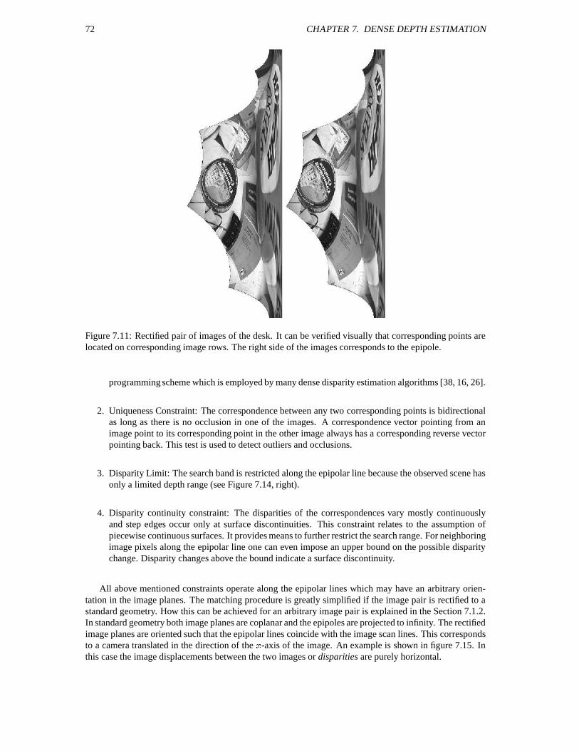
72 CHAPTER 7. DENSE DEPTH ESTIMATION
Figure 7.11: Rectified pair of images of the desk. It can be verified visually that corresponding points arelocated on corresponding image rows. The right side of the images corresponds to the epipole.
programming scheme which is employed by many dense disparity estimation algorithms [38, 16, 26].
2. Uniqueness Constraint: The correspondence between any two corresponding points is bidirectionalas long as there is no occlusion in one of the images. A correspondence vector pointing from animage point to its corresponding point in the other image always has a corresponding reverse vectorpointing back. This test is used to detect outliers and occlusions.
3. Disparity Limit: The search band is restricted along the epipolar line because the observed scene hasonly a limited depth range (see Figure 7.14, right).
4. Disparity continuity constraint: The disparities of the correspondences vary mostly continuouslyand step edges occur only at surface discontinuities. This constraint relates to the assumption ofpiecewise continuous surfaces. It provides means to further restrict the search range. For neighboringimage pixels along the epipolar line one can even impose an upper bound on the possible disparitychange. Disparity changes above the bound indicate a surface discontinuity.
All above mentioned constraints operate along the epipolar lines which may have an arbitrary orien-tation in the image planes. The matching procedure is greatly simplified if the image pair is rectified to astandard geometry. How this can be achieved for an arbitrary image pair is explained in the Section 7.1.2.In standard geometry both image planes are coplanar and the epipoles are projected to infinity. The rectifiedimage planes are oriented such that the epipolar lines coincide with the image scan lines. This correspondsto a camera translated in the direction of the 3 -axis of the image. An example is shown in figure 7.15. Inthis case the image displacements between the two images or disparities are purely horizontal.
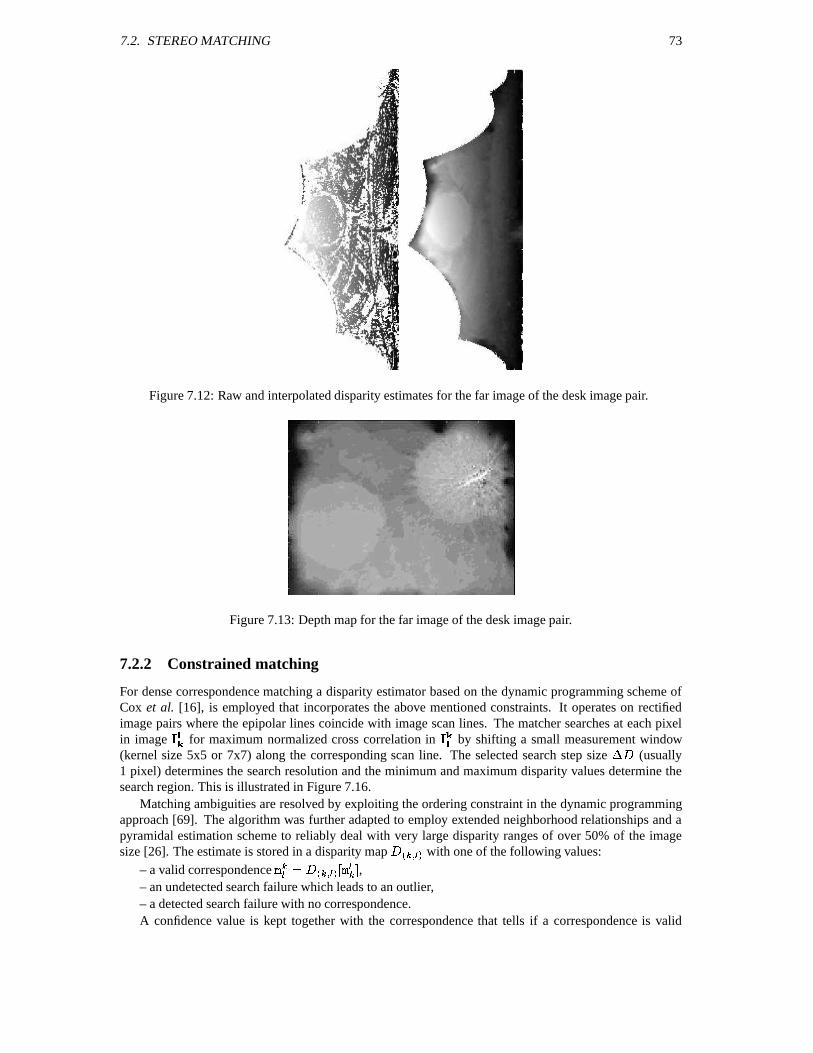
7.2. STEREO MATCHING 73
Figure 7.12: Raw and interpolated disparity estimates for the far image of the desk image pair.
Figure 7.13: Depth map for the far image of the desk image pair.
7.2.2 Constrained matching
For dense correspondence matching a disparity estimator based on the dynamic programming scheme ofCox et al. [16], is employed that incorporates the above mentioned constraints. It operates on rectifiedimage pairs where the epipolar lines coincide with image scan lines. The matcher searches at each pixelin image \
for maximum normalized cross correlation in \
by shifting a small measurement window(kernel size 5x5 or 7x7) along the corresponding scan line. The selected search step size
(usually
1 pixel) determines the search resolution and the minimum and maximum disparity values determine thesearch region. This is illustrated in Figure 7.16.
Matching ambiguities are resolved by exploiting the ordering constraint in the dynamic programmingapproach [69]. The algorithm was further adapted to employ extended neighborhood relationships and apyramidal estimation scheme to reliably deal with very large disparity ranges of over 50% of the imagesize [26]. The estimate is stored in a disparity map
F with one of the following values:– a valid correspondence F & F 1 F 5 ,– an undetected search failure which leads to an outlier,– a detected search failure with no correspondence.A confidence value is kept together with the correspondence that tells if a correspondence is valid
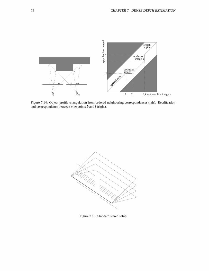
74 CHAPTER 7. DENSE DEPTH ESTIMATION
1 4
1 2 1,23,4 3 4
2 3
P Pk k+1
optim
al pa
th
epipolar line image k1 2 3,4
1,2 image l
searchregion
epip
olar
line
imag
e l
image kocclusion
occlusion
3
4
Figure 7.14: Object profile triangulation from ordered neighboring correspondences (left). Rectificationand correspondence between viewpoints and (right).
Figure 7.15: Standard stereo setup
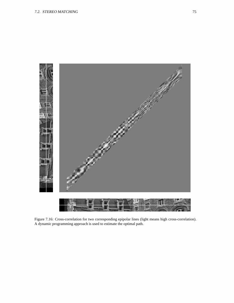
7.2. STEREO MATCHING 75
Figure 7.16: Cross-correlation for two corresponding epipolar lines (light means high cross-correlation).A dynamic programming approach is used to estimate the optimal path.
76 CHAPTER 7. DENSE DEPTH ESTIMATION
and how good it is. The confidence is derived from the local image variance and the maximum crosscorrelation[73]. To further reduce measurement outliers the uniqueness constraint is employed by estimat-ing correspondences bidirectionally
N HC P YN !C P . Only the consistent correspondences with YN HC P YN !C P are kept as valid correspondences.
7.3 Multi-view stereo
The pairwise disparity estimation allows to compute image to image correspondences between adjacentrectified image pairs, and independent depth estimates for each camera viewpoint. An optimal joint esti-mate will be achieved by fusing all independent estimates into a common 3D model. The fusion can beperformed in an economical way through controlled correspondence linking as described in this section.The approach utilizes a flexible multi-viewpoint scheme by combining the advantages of small baselineand wide baseline stereo.
As small baseline stereo we define viewpoints where the baseline is much smaller than the observedaverage scene depth. This configuration is usually valid for image sequences were the images are taken asa spatial sequence from many slightly varying view-points. The advantages (+) and disadvantages (–) are
+ easy correspondence estimation, since the views are similar,+ small regions of viewpoint related occlusions1,– small triangulation angle, hence large depth uncertainty.The wide baseline stereo in contrast is used mostly with still image photographs of a scene where few
images are taken from a very different viewpoint. Here the depth resolution is superior but correspondenceand occlusion problems appear:
– hard correspondence estimation, since the views are not similar,– large regions of viewpoint related occlusions,+ big triangulation angle, hence high depth accuracy.The multi-viewpoint linking combines the virtues of both approaches. In addition it will produce
denser depth maps than either of the other techniques, and allows additional features for depth and texturefusion. Advantages are:
+ very dense depth maps for each viewpoint,+ no viewpoint dependent occlusions,+ highest depth resolution through viewpoint fusion,+ texture enhancement (mean texture, highlight removal, super-resolution texture).
7.3.1 Correspondence Linking Algorithm
The correspondence linking is described in this section. It concatenates corresponding image points overmultiple viewpoints by correspondence tracking over adjacent image pairs. This of course implies thatthe individually measured pair matches are accurate. To account for outliers in pair matches, some ro-bust control strategies need to be employed to check the validity of the correspondence linking. Consideran image sequence taken from 4& 1 5 viewpoints. Assume that the sequence is taken by a cameramoving sideways while keeping the object in view. For any view point let us consider the image triple1 \ UZW \ \ 4 W 5 . The image pairs ( \ UXW , \ ) and ( \ , \ 4 W ) form two stereoscopic image pairs with cor-respondence estimates as described above. We have now defined 3 representations of image and cameramatrices for each viewpoint: the original image \ and projection matrix
, their transformed versions\ UXW UZW rectified towards view point with transformation
" UZW and the transformed \ 4 W 4 Wrectified towards viewpoint . with mapping
" 4 W . The Disparity map UXW holds the downward
correspondences from \ UZW to \ UXW while the map 4 W contains the upward correspondences from
\ 4 W to \ 4 W . We can now create two chains of correspondence links for an image point , one up andone down the image index .
1As view point related occlusions we consider those parts of the object that are visible in one image only, due to object self-occlusion.
7.3. MULTI-VIEW STEREO 77
Upwards linking: 4 & N " 4 W P UZW 4 W 1" 4 W 5
Downwards linking: U & N " UZW P UXW UXW 1 " UZW 5This linking process is repeated along the image sequence to create a chain of correspondences upwards
and downwards. Every correspondence link requires 2 mappings and 1 disparity lookup. Throughoutthe sequence of N images, N
Pdisparity maps are computed. The multi-viewpoint linking is then
performed efficiently via fast lookup functions on the pre-computed estimates.Due to the rectification mapping transformed image point will normally not fall on integer pixel co-
ordinates in the rectified image. The lookup of an image disparity in the disparity map D will thereforerequire an interpolation function. Since disparity maps for piecewise continuous surfaces have a spatiallylow frequency content, a bilinear interpolation between pixels suffices.
Occlusions and visibility
In a triangulation sensor with two viewpoints and two types of occlusion occur. If parts of the object arehidden in both viewpoints due to object self-occlusion, then we speak of object occlusions which cannot beresolved from this viewpoint. If a surface region is visible in viewpoint but not in , we speak of a shadowocclusion. The regions have a shadow-like appearance of undefined disparity values since the occlusionsat view cast a shadow on the object as seen from view . Shadow occlusions are in fact detected by theuniqueness constraint discussed in section 7.2. A solution to avoid shadow occlusions is to incorporatea symmetrical multi-viewpoint matcher as proposed in this contribution. Points that are shadowed in the(right) view . are normally visible in the (left) view and vice versa. The exploitation of up-and down-links will resolve for most of the shadow occlusions. A helpful measure in this context is thevisibility V that defines for a pixel in view the maximum number of possible correspondences in thesequence.
& is caused by a shadow occlusion, & allows a depth estimate.
Depth estimation and outlier detection
Care must be taken to exclude invalid disparity values or outliers from the chain. If an invalid disparityvalue is encountered, the chain is terminated immediately. Outliers are detected by controlling the statisticsof the depth estimate computed from the correspondences. Inliers will update the depth estimate using a1-D Kalman filter.
Depth and uncertainty Assume a 3D surface point
that is projected onto its corresponding imagepoints & F & F . The inverse process holds for triangulating
from the corresponding point
pairN F P . We can in fact exploit the calibrated camera geometry and express the 3D point
as a depth
value along the known line of sight that extends from the camera projection center through the image
correspondence . Triangulation computes the depth as the length of connecting the camera projectioncenter and the locus of minimum distance between the corresponding lines of sight. The triangulation iscomputed for each image point and stored in a dense depth map associated with the viewpoint.
The depth for each reference image point 0 is improved by the correspondence linking that deliverstwo lists of image correspondences relative to the reference, one linking down from HC and one linkingup from C . For each valid corresponding point pair
N P we can triangulate a consistent depthestimate
N 9F P along with F representing the depth uncertainty. Figure 7.17(left) visualizes thedecreasing uncertainty interval during linking. While the disparity measurement resolution
in the
image is kept constant (at 1 pixel), the reprojected depth error F decreases with the baseline.
Outlier detection and inlier fusion As measurement noise we assume a contaminated Gaussian distri-bution with a main peak within a small interval (of 1 pixel) and a small percentage of outliers. Inlier noiseis caused by the limited resolution of the disparity matcher and by the interpolation artifacts. Outliers areundetected correspondence failures and may be arbitrarily large. As threshold to detect the outliers weutilize the depth uncertainty interval . The detection of an outlier at terminates the linking at .All depth values 1 4 W F UZW65 are inlier depth values that fall within the uncertainty interval around
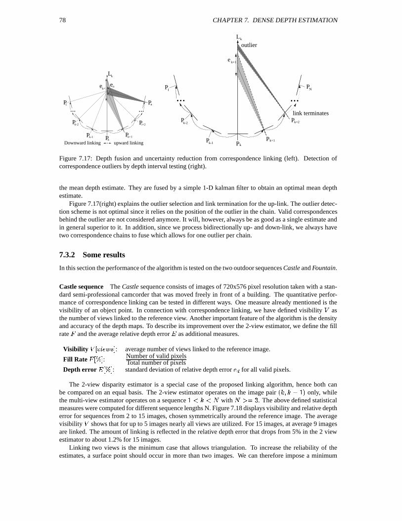
78 CHAPTER 7. DENSE DEPTH ESTIMATION
ne
kL
e
......P1
P Pi+2
nP
k+1
k+1P
k-2
Pk-1 PkDownward linking upward linking
P
P
...P
P
e k+1
P
P
P
1 N
kLoutlier
link terminatesk+2
...
k-2
k-1k
k+1
Figure 7.17: Depth fusion and uncertainty reduction from correspondence linking (left). Detection ofcorrespondence outliers by depth interval testing (right).
the mean depth estimate. They are fused by a simple 1-D kalman filter to obtain an optimal mean depthestimate.
Figure 7.17(right) explains the outlier selection and link termination for the up-link. The outlier detec-tion scheme is not optimal since it relies on the position of the outlier in the chain. Valid correspondencesbehind the outlier are not considered anymore. It will, however, always be as good as a single estimate andin general superior to it. In addition, since we process bidirectionally up- and down-link, we always havetwo correspondence chains to fuse which allows for one outlier per chain.
7.3.2 Some results
In this section the performance of the algorithm is tested on the two outdoor sequences Castle and Fountain.
Castle sequence The Castle sequence consists of images of 720x576 pixel resolution taken with a stan-dard semi-professional camcorder that was moved freely in front of a building. The quantitative perfor-mance of correspondence linking can be tested in different ways. One measure already mentioned is thevisibility of an object point. In connection with correspondence linking, we have defined visibility
as
the number of views linked to the reference view. Another important feature of the algorithm is the densityand accuracy of the depth maps. To describe its improvement over the 2-view estimator, we define the fillrate and the average relative depth error as additional measures.
Visibility 1 5 : average number of views linked to the reference image.
Fill Rate H1 5 : Number of valid pixelsTotal number of pixels
Depth error B1 5 : standard deviation of relative depth error for all valid pixels.
The 2-view disparity estimator is a special case of the proposed linking algorithm, hence both canbe compared on an equal basis. The 2-view estimator operates on the image pair
N . P
only, whilethe multi-view estimator operates on a sequence
with & . The above defined statisticalmeasures were computed for different sequence lengths N. Figure 7.18 displays visibility and relative deptherror for sequences from 2 to 15 images, chosen symmetrically around the reference image. The averagevisibility
shows that for up to 5 images nearly all views are utilized. For 15 images, at average 9 images
are linked. The amount of linking is reflected in the relative depth error that drops from 5% in the 2 viewestimator to about 1.2% for 15 images.
Linking two views is the minimum case that allows triangulation. To increase the reliability of theestimates, a surface point should occur in more than two images. We can therefore impose a minimum

7.3. MULTI-VIEW STEREO 79
2 3 5 7 9 11 13 150
1
2
3
4
5
E [%
]
2 3 4 50
1
2
3
4
5
E [%
]2 3 5 7 9 11 13 15
0
2
4
6
8
10
N [view]
V [v
iew
]
2 3 4 50
20
40
60
80
100
Vmin [view]
F [%
]
Figure 7.18: Statistics of the castle sequence. Influence of sequence length on visibility
and relativedepth error . (left) Influence of minimum visibility
>. on fill rate and depth error for &
(center). Depth map (above: dark=near, light=far) and error map (below: dark=large error, light=smallerror) for & and
>. &) (right).
visibility
>. on a depth estimate. This will reject unreliable depth estimates effectively, but will also
reduce the fill rate of the depth map.The graphs in figure 7.18(center) show the dependency of the fill rate and depth error on minimum
visibility for N=11. The fill rate drops from 92% to about 70%, but at the same time the depth error isreduced to 0.5% due to outlier rejection. The depth map and the relative error distribution over the depthmap is displayed in Figure 7.18(right). The error distribution shows a periodic structure that in fact reflectsthe quantization uncertainty of the disparity resolution when it switches from one disparity value to thenext.
Fountain sequence The Fountain sequence consists of 5 images of the back wall of the Upper Agora atthe archaeological site of Sagalassos in Turkey, taken with a digital camera with 573x764 pixel resolution.It shows a concavity in which once a statue was situated.
N[view] 1 5 H1 5 B1 5
2 2 89.8728 0.2944033 2.85478 96.7405 0.2083675 4.23782 96.4774 0.121955
Table 7.1: Statistics of the fountain sequence for visibility
, fill rate and depth error .
The performance characteristics are displayed in the table 7.1. The fill rate is high and the relativeerror is rather low because of a fairly wide baseline between views. This is reflected in the high geometricquality of depth the map and the reconstruction. Figure 7.19 shows from left to right images 1 and 3 ofthe sequence, the depth map as computed with the 2-view estimator, and the depth map when using all 5images. The white (undefined) regions in the 2-view depth map are due to shadow occlusions which arealmost completely removed in the 5-view depth map. This is reflected in the fill rate that increases from 89to 96%. It should be noted that for this sequence a very large search range of 400 pixels was used, whichis over 70% of the image width. Despite this large search range only few matching errors occurred.
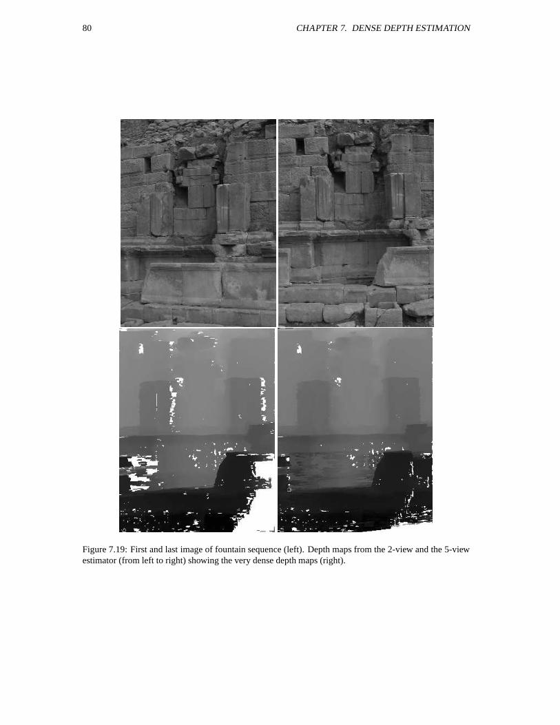
80 CHAPTER 7. DENSE DEPTH ESTIMATION
Figure 7.19: First and last image of fountain sequence (left). Depth maps from the 2-view and the 5-viewestimator (from left to right) showing the very dense depth maps (right).
7.4. CONCLUSION 81
7.4 Conclusion
In this chapter we presented a scheme that computes dense and accurate depth maps based on the sequencelinking of pairwise estimated disparity maps. First a matching algorithm was presented which computescorresponding points for an image pair in standard stereo configuration. Then it was explained how imagescan be rectified so that any pair of images can be brought to this configuration. Finally a multi-view linkingapproach was presented which allows to combine the results to obtain more accurate and dense depth maps.The performance analysis showed that very dense depth maps with fill rates of over 90 % and a relativedepth error of 0.1% can be measured with off-the-shelf cameras even in unrestricted outdoor environmentssuch as an archaeological site.

82 CHAPTER 7. DENSE DEPTH ESTIMATION
Chapter 8
Modeling
In the previous chapters we have seen how the information needed to build a 3D model could automaticallybe obtained from images. This chapter explains how this information can be combined to build realisticrepresentations of the scene. It is not only possible to generate a surface model or volumetric model easily,but all the necessary information is available to build lightfield models or even augmented video sequences.These different cases will now be discussed in more detail.
8.1 Surface model
The 3D surface is approximated by a triangular mesh to reduce geometric complexity and to tailor themodel to the requirements of computer graphics visualization systems. A simple approach consists ofoverlaying a 2D triangular mesh on top of the image and then build a corresponding 3D mesh by placingthe vertices of the triangles in 3D space according to the values found in the depth map. To reduce noiseit is recommended to first smooth the depth image (the kernel can be chosen of the same size as the meshtriangles). The image itself can be used as texture map (the texture coordinates are trivially obtained as the2D coordinates of the vertices).
It can happen that for some vertices no depth value is available or that the confidence is too low (seeSection 7.2.2). In these cases the corresponding triangles are not reconstructed. The same happens whentriangles are placed over discontinuities. This is achieved by selecting a maximum angle between thenormal of a triangle and the line of sight through its center (e.g. 85 degrees).
This simple approach works very well on the depth maps obtained after multi-view linking. On simplestereo depth maps it is recommended to use a more advanced technique described in [73]. In this case theboundaries of the objects to be modeled are computed through depth segmentation. In a first step, an objectis defined as a connected region in space. Simple morphological filtering removes spurious and very smallregions. Then a bounded thin plate model is employed with a second order spline to smooth the surfaceand to interpolate small surface gaps in regions that could not be measured.
The surface reconstruction approach is illustrated in Figure 8.1. The obtained 3D surface model isshown in Figure 8.2 with shading and with texture. Note that this surface model is reconstructed from theviewpoint of a reference image. If the whole scene can not be seen from one image, it it necessary to applya technique to fuse different surfaces together (e.g. [162, 19]).
8.1.1 Texture enhancement
The correspondence linking builds a controlled chain of correspondences that can be used for texture en-hancement as well. At each reference pixel one may collect a sorted list of image color values from thecorresponding image positions. This allows to enhance the original texture in many ways by accessing thecolor statistics. Some features that are derived naturally from the linking algorithm are:
83
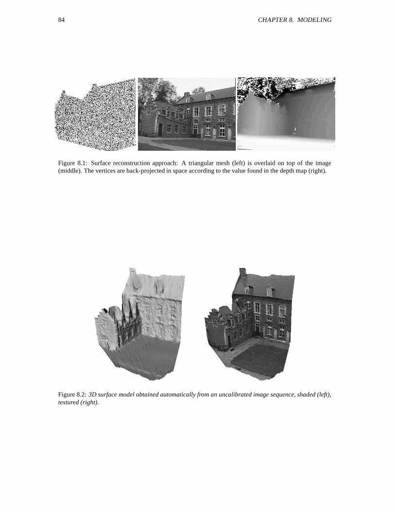
84 CHAPTER 8. MODELING
Figure 8.1: Surface reconstruction approach: A triangular mesh (left) is overlaid on top of the image(middle). The vertices are back-projected in space according to the value found in the depth map (right).
Figure 8.2: 3D surface model obtained automatically from an uncalibrated image sequence, shaded (left),textured (right).
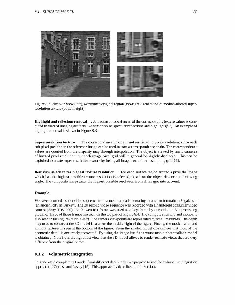
8.1. SURFACE MODEL 85
Figure 8.3: close-up view (left), 4x zoomed original region (top-right), generation of median-filtered super-resolution texture (bottom-right).
Highlight and reflection removal : A median or robust mean of the corresponding texture values is com-puted to discard imaging artifacts like sensor noise, specular reflections and highlights[93]. An example ofhighlight removal is shown in Figure 8.3.
Super-resolution texture : The correspondence linking is not restricted to pixel-resolution, since eachsub-pixel-position in the reference image can be used to start a correspondence chain. The correspondencevalues are queried from the disparity map through interpolation. The object is viewed by many camerasof limited pixel resolution, but each image pixel grid will in general be slightly displaced. This can beexploited to create super-resolution texture by fusing all images on a finer resampling grid[61].
Best view selection for highest texture resolution : For each surface region around a pixel the imagewhich has the highest possible texture resolution is selected, based on the object distance and viewingangle. The composite image takes the highest possible resolution from all images into account.
Example
We have recorded a short video sequence from a medusa head decorating an ancient fountain in Sagalassos(an ancient city in Turkey). The 20 second video sequence was recorded with a hand-held consumer videocamera (Sony TRV-900). Each twentiest frame was used as a key-frame by our video to 3D processingpipeline. Three of these frames are seen on the top part of Figure 8.4. The compute structure and motion isalso seen in this figure (middle-left). The camera viewpoints are represented by small pyramids. The depthmap used to construct the 3D model is seen on the middle-right of the figure. Finally, the model -with andwithout texture- is seen at the bottom of the figure. From the shaded model one can see that most of thegeometric detail is accurately recovered. By using the image itself as texture map a photorealistic modelis obtained. Note from the rightmost view that the 3D model allows to render realistic views that are verydifferent from the original views.
8.1.2 Volumetric integration
To generate a complete 3D model from different depth maps we propose to use the volumetric integrationapproach of Curless and Levoy [19]. This approach is described in this section.
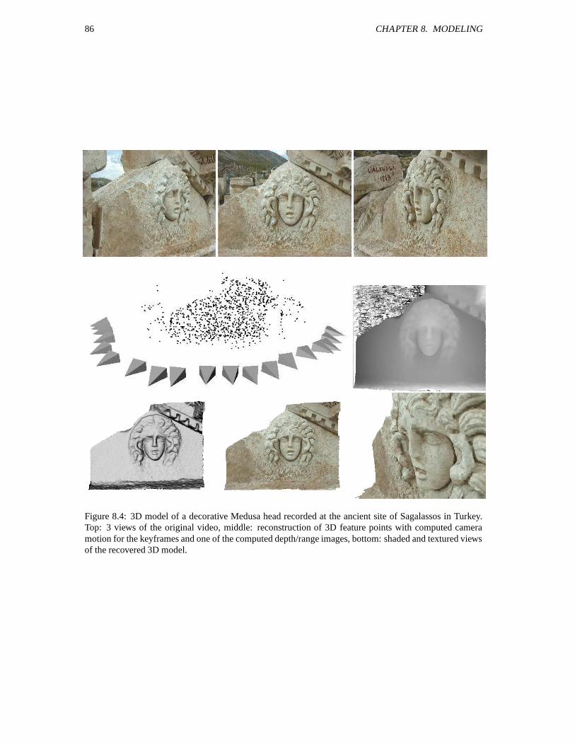
86 CHAPTER 8. MODELING
Figure 8.4: 3D model of a decorative Medusa head recorded at the ancient site of Sagalassos in Turkey.Top: 3 views of the original video, middle: reconstruction of 3D feature points with computed cameramotion for the keyframes and one of the computed depth/range images, bottom: shaded and textured viewsof the recovered 3D model.
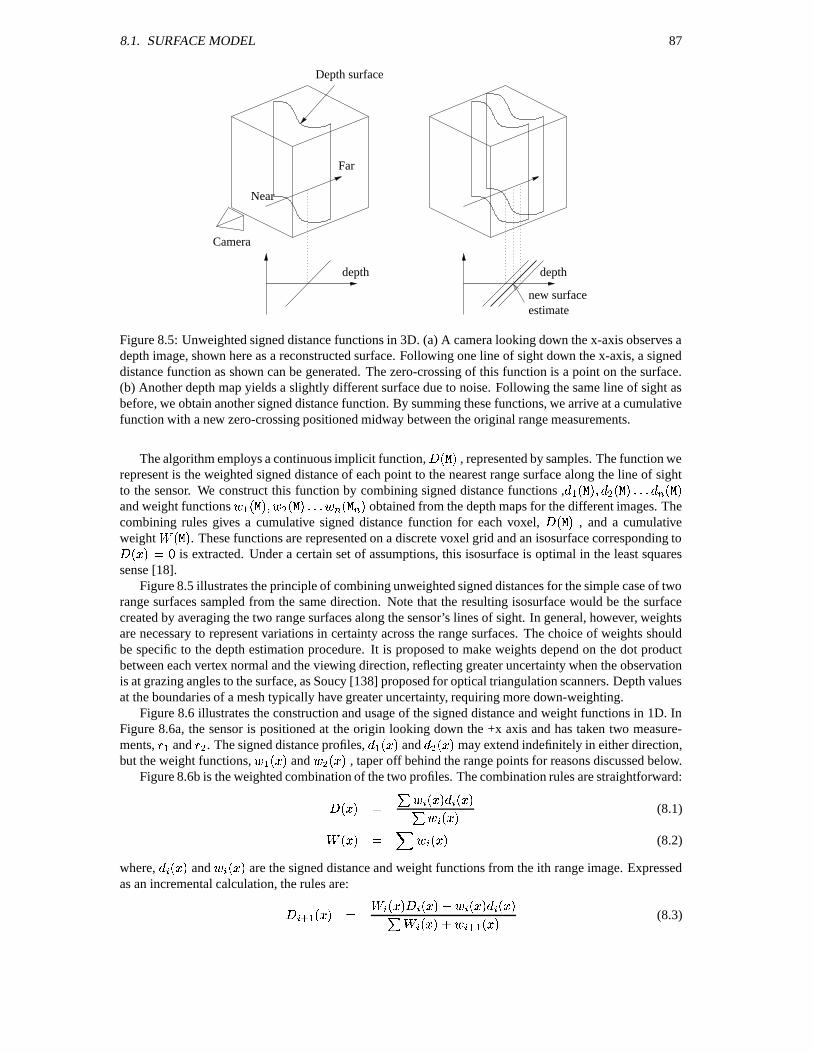
8.1. SURFACE MODEL 87
Depth surface
Near
Far
Camera
depth depth
new surfaceestimate
Figure 8.5: Unweighted signed distance functions in 3D. (a) A camera looking down the x-axis observes adepth image, shown here as a reconstructed surface. Following one line of sight down the x-axis, a signeddistance function as shown can be generated. The zero-crossing of this function is a point on the surface.(b) Another depth map yields a slightly different surface due to noise. Following the same line of sight asbefore, we obtain another signed distance function. By summing these functions, we arrive at a cumulativefunction with a new zero-crossing positioned midway between the original range measurements.
The algorithm employs a continuous implicit function,YN P
, represented by samples. The function werepresent is the weighted signed distance of each point to the nearest range surface along the line of sightto the sensor. We construct this function by combining signed distance functions ,
W N P , N P . N Pand weight functions W N P , N P . N . P obtained from the depth maps for the different images. Thecombining rules gives a cumulative signed distance function for each voxel,
YN P, and a cumulative
weight % N P . These functions are represented on a discrete voxel grid and an isosurface corresponding toYN 3 P & ( is extracted. Under a certain set of assumptions, this isosurface is optimal in the least squaressense [18].
Figure 8.5 illustrates the principle of combining unweighted signed distances for the simple case of tworange surfaces sampled from the same direction. Note that the resulting isosurface would be the surfacecreated by averaging the two range surfaces along the sensor’s lines of sight. In general, however, weightsare necessary to represent variations in certainty across the range surfaces. The choice of weights shouldbe specific to the depth estimation procedure. It is proposed to make weights depend on the dot productbetween each vertex normal and the viewing direction, reflecting greater uncertainty when the observationis at grazing angles to the surface, as Soucy [138] proposed for optical triangulation scanners. Depth valuesat the boundaries of a mesh typically have greater uncertainty, requiring more down-weighting.
Figure 8.6 illustrates the construction and usage of the signed distance and weight functions in 1D. InFigure 8.6a, the sensor is positioned at the origin looking down the +x axis and has taken two measure-ments,
W and, . The signed distance profiles,
W N 3 P and,N 3 P may extend indefinitely in either direction,
but the weight functions, W N 3 P and , N 3 P , taper off behind the range points for reasons discussed below.Figure 8.6b is the weighted combination of the two profiles. The combination rules are straightforward:YN 3 P & K N 3 P N 3 P
K N 3 P (8.1)
% N 3 P & L N 3 P (8.2)
where, N 3 P and N 3 P are the signed distance and weight functions from the ith range image. Expressed
as an incremental calculation, the rules are: 4 WN 3 P & % N 3 P N 3 P . N 3 P N 3 P
K % N 3 P . 4 W N 3 P (8.3)
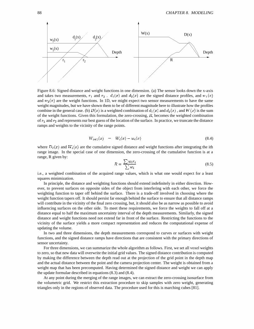
88 CHAPTER 8. MODELING
Depth
W(x) D(x)
R
Depth
d (x) d (x)1 2
w (x)1
r1 r2
2w (x)
Figure 8.6: Signed distance and weight functions in one dimension. (a) The sensor looks down the x-axisand takes two measurements,
W and, .
W N 3 P and,N 3 P are the signed distance profiles, and W N 3 P
and , N 3 P are the weight functions. In 1D, we might expect two sensor measurements to have the sameweight magnitudes, but we have shown them to be of different magnitude here to illustrate how the profilescombine in the general case. (b)
N 3 P is a weighted combination of W N 3 P and
,N 3 P , and % N 3 P is the sum
of the weight functions. Given this formulation, the zero-crossing, , becomes the weighted combinationof W and
, and represents our best guess of the location of the surface. In practice, we truncate the distance
ramps and weights to the vicinity of the range points.
% 4 WN 3 P & % N 3 P . N 3 P (8.4)
where N 3 P and % N 3 P are the cumulative signed distance and weight functions after integrating the ith
range image. In the special case of one dimension, the zero-crossing of the cumulative function is at arange, R given by:
& K K (8.5)
i.e., a weighted combination of the acquired range values, which is what one would expect for a leastsquares minimization.
In principle, the distance and weighting functions should extend indefinitely in either direction. How-ever, to prevent surfaces on opposite sides of the object from interfering with each other, we force theweighting function to taper off behind the surface. There is a trade-off involved in choosing where theweight function tapers off. It should persist far enough behind the surface to ensure that all distance rampswill contribute in the vicinity of the final zero crossing, but, it should also be as narrow as possible to avoidinfluencing surfaces on the other side. To meet these requirements, we force the weights to fall off at adistance equal to half the maximum uncertainty interval of the depth measurements. Similarly, the signeddistance and weight functions need not extend far in front of the surface. Restricting the functions to thevicinity of the surface yields a more compact representation and reduces the computational expense ofupdating the volume.
In two and three dimensions, the depth measurements correspond to curves or surfaces with weightfunctions, and the signed distance ramps have directions that are consistent with the primary directions ofsensor uncertainty.
For three dimensions, we can summarize the whole algorithm as follows. First, we set all voxel weightsto zero, so that new data will overwrite the initial grid values. The signed distance contribution is computedby making the difference between the depth read out at the projection of the grid point in the depth mapand the actual distance between the point and the camera projection center. The weight is obtained from aweight map that has been precomputed. Having determined the signed distance and weight we can applythe update formulae described in equations (8.3) and (8.4).
At any point during the merging of the range images, we can extract the zero-crossing isosurface fromthe volumetric grid. We restrict this extraction procedure to skip samples with zero weight, generatingtriangles only in the regions of observed data. The procedure used for this is marching cubes [81].
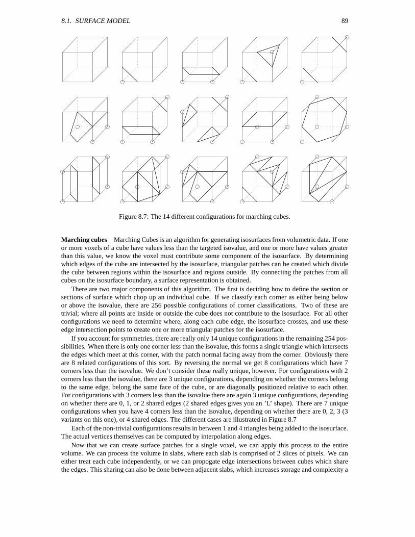
8.1. SURFACE MODEL 89
Figure 8.7: The 14 different configurations for marching cubes.
Marching cubes Marching Cubes is an algorithm for generating isosurfaces from volumetric data. If oneor more voxels of a cube have values less than the targeted isovalue, and one or more have values greaterthan this value, we know the voxel must contribute some component of the isosurface. By determiningwhich edges of the cube are intersected by the isosurface, triangular patches can be created which dividethe cube between regions within the isosurface and regions outside. By connecting the patches from allcubes on the isosurface boundary, a surface representation is obtained.
There are two major components of this algorithm. The first is deciding how to define the section orsections of surface which chop up an individual cube. If we classify each corner as either being belowor above the isovalue, there are 256 possible configurations of corner classifications. Two of these aretrivial; where all points are inside or outside the cube does not contribute to the isosurface. For all otherconfigurations we need to determine where, along each cube edge, the isosurface crosses, and use theseedge intersection points to create one or more triangular patches for the isosurface.
If you account for symmetries, there are really only 14 unique configurations in the remaining 254 pos-sibilities. When there is only one corner less than the isovalue, this forms a single triangle which intersectsthe edges which meet at this corner, with the patch normal facing away from the corner. Obviously thereare 8 related configurations of this sort. By reversing the normal we get 8 configurations which have 7corners less than the isovalue. We don’t consider these really unique, however. For configurations with 2corners less than the isovalue, there are 3 unique configurations, depending on whether the corners belongto the same edge, belong the same face of the cube, or are diagonally positioned relative to each other.For configurations with 3 corners less than the isovalue there are again 3 unique configurations, dependingon whether there are 0, 1, or 2 shared edges (2 shared edges gives you an ’L’ shape). There are 7 uniqueconfigurations when you have 4 corners less than the isovalue, depending on whether there are 0, 2, 3 (3variants on this one), or 4 shared edges. The different cases are illustrated in Figure 8.7
Each of the non-trivial configurations results in between 1 and 4 triangles being added to the isosurface.The actual vertices themselves can be computed by interpolation along edges.
Now that we can create surface patches for a single voxel, we can apply this process to the entirevolume. We can process the volume in slabs, where each slab is comprised of 2 slices of pixels. We caneither treat each cube independently, or we can propogate edge intersections between cubes which sharethe edges. This sharing can also be done between adjacent slabs, which increases storage and complexity a
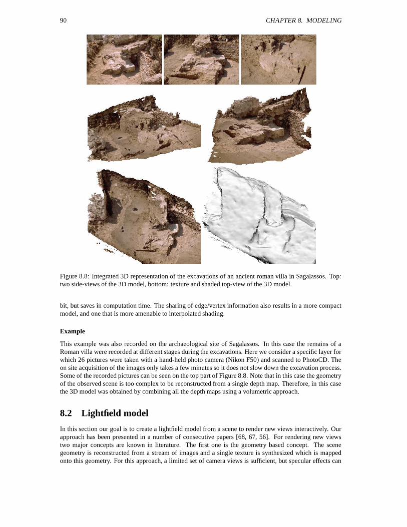
90 CHAPTER 8. MODELING
Figure 8.8: Integrated 3D representation of the excavations of an ancient roman villa in Sagalassos. Top:two side-views of the 3D model, bottom: texture and shaded top-view of the 3D model.
bit, but saves in computation time. The sharing of edge/vertex information also results in a more compactmodel, and one that is more amenable to interpolated shading.
Example
This example was also recorded on the archaeological site of Sagalassos. In this case the remains of aRoman villa were recorded at different stages during the excavations. Here we consider a specific layer forwhich 26 pictures were taken with a hand-held photo camera (Nikon F50) and scanned to PhotoCD. Theon site acquisition of the images only takes a few minutes so it does not slow down the excavation process.Some of the recorded pictures can be seen on the top part of Figure 8.8. Note that in this case the geometryof the observed scene is too complex to be reconstructed from a single depth map. Therefore, in this casethe 3D model was obtained by combining all the depth maps using a volumetric approach.
8.2 Lightfield model
In this section our goal is to create a lightfield model from a scene to render new views interactively. Ourapproach has been presented in a number of consecutive papers [68, 67, 56]. For rendering new viewstwo major concepts are known in literature. The first one is the geometry based concept. The scenegeometry is reconstructed from a stream of images and a single texture is synthesized which is mappedonto this geometry. For this approach, a limited set of camera views is sufficient, but specular effects can
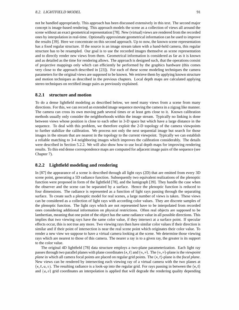
8.2. LIGHTFIELD MODEL 91
not be handled appropriately. This approach has been discussed extensively in this text. The second majorconcept is image-based rendering. This approach models the scene as a collection of views all around thescene without an exact geometrical representation [78]. New (virtual) views are rendered from the recordedones by interpolation in real-time. Optionally approximate geometrical information can be used to improvethe results [39]. Here we concentrate on this second approach. Up to now, the known scene representationhas a fixed regular structure. If the source is an image stream taken with a hand-held camera, this regularstructure has to be resampled. Our goal is to use the recorded images themselve as scene representationand to directly render new views from them. Geometrical information is considered as far as it is knownand as detailed as the time for rendering allows. The approach is designed such, that the operations consistof projective mappings only which can efficiently be performed by the graphics hardware (this comesvery close to the approach described in [23]). For each of these scene modeling techniques the cameraparameters for the original views are supposed to be known. We retrieve them by applying known structureand motion techniques as described in the previous chapters. Local depth maps are calculated applyingstereo techniques on rectified image pairs as previously explained.
8.2.1 structure and motion
To do a dense lightfield modeling as described below, we need many views from a scene from manydirections. For this, we can record an extended image sequence moving the camera in a zigzag like manner.The camera can cross its own moving path several times or at least gets close to it. Known calibrationmethods usually only consider the neighborhoods within the image stream. Typically no linking is donebetween views whose position is close to each other in 3-D space but which have a large distance in thesequence. To deal with this problem, we therefore exploit the 2-D topology of the camera viewpointsto further stabilize the calibration. We process not only the next sequential image but search for thoseimages in the stream that are nearest in the topology to the current viewpoint. Typically we can establisha reliable matching to 3-4 neighboring images which improves the calibration considerably. The detailswere described in Section 5.2.2. We will also show how to use local depth maps for improving renderingresults. To this end dense correspondence maps are computed for adjacent image pairs of the sequence (seeChapter 7).
8.2.2 Lightfield modeling and rendering
In [87] the appearance of a scene is described through all light rays (2D) that are emitted from every 3Dscene point, generating a 5D radiance function. Subsequently two equivalent realizations of the plenopticfunction were proposed in form of the lightfield [78], and the lumigraph [39]. They handle the case whenthe observer and the scene can be separated by a surface. Hence the plenoptic function is reduced tofour dimensions. The radiance is represented as a function of light rays passing through the separatingsurface. To create such a plenoptic model for real scenes, a large number of views is taken. These viewscan be considered as a collection of light rays with according color values. They are discrete samples ofthe plenoptic function. The light rays which are not represented have to be interpolated from recordedones considering additional information on physical restrictions. Often real objects are supposed to belambertian, meaning that one point of the object has the same radiance value in all possible directions. Thisimplies that two viewing rays have the same color value, if they intersect at a surface point. If speculareffects occur, this is not true any more. Two viewing rays then have similar color values if their direction issimilar and if their point of intersection is near the real scene point which originates their color value. Torender a new view we suppose to have a virtual camera looking at the scene. We determine those viewingrays which are nearest to those of this camera. The nearer a ray is to a given ray, the greater is its supportto the color value.
The original 4D lightfield [78] data structure employs a two-plane parameterization. Each light raypasses through two parallel planes with plane coordinates
N P andN P . The
N P -plane is the viewpointplane in which all camera focal points are placed on regular grid points. The
N P -plane is the focal plane.New views can be rendered by intersecting each viewing ray of a virtual camera with the two planes atN P . The resulting radiance is a look-up into the regular grid. For rays passing in between the
N Pand
N P grid coordinates an interpolation is applied that will degrade the rendering quality depending

92 CHAPTER 8. MODELING
on the scene geometry. In fact, the lightfield contains an implicit geometrical assumption, i.e. the scenegeometry is planar and coincides with the focal plane. Deviation of the scene geometry from the focalplane causes image degradation (i.e. blurring or ghosting). To use hand-held camera images, the solutionproposed in [39] consists of rebinning the images to the regular grid. The disadvantage of this rebinningstep is that the interpolated regular structure already contains inconsistencies and ghosting artifacts becauseof errors in the scantily approximated geometry. During rendering the effect of ghosting artifacts is repeatedso duplicate ghosting effects occur.
Rendering from recorded images Our goal is to overcome the problems described in the last section byrelaxing the restrictions imposed by the regular lightfield structure and to render views directly from thecalibrated sequence of recorded images with use of local depth maps. Without loosing performance theoriginal images are directly mapped onto one or more planes viewed by a virtual camera.
To obtain a high-quality image-based scene representation, we need many views from a scene frommany directions. For this, we can record an extended image sequence moving the camera in a zigzaglike manner. The camera can cross its own moving path several times or at least gets close to it. Toobtain a good quality structure-and-motion estimation from this type of sequence it is important to usethe extensions proposed in Section 5.2 to match close views that are not predecessors or successors inthe image stream. To allow to construct the local geometrical approximation depth maps should also becomputed as described in the previous section.
Fixed plane approximation In a first approach, we approximate the scene geometry by a single plane by minimizing the least square error. We map all given camera images onto plane and view it througha virtual camera. This can be achieved by directly mapping the coordinates 3 8 of image onto thevirtual camera coordinates 1 3 8 5 S & 1 3 8 5 S . Therefore we can perform a direct look-up intothe originally recorded images and determine the radiance by interpolating the recorded neighboring pixelvalues. This technique is similar to the lightfield approach [78] which implicitly assumes the focal planeas the plane of geometry. Thus to construct a specific view we have to interpolate between neighboringviews. Those views give the most support to the color value of a particular pixel whose projection centeris close to the viewing ray of this pixel. This is equivalent to the fact that those views whose projectedcamera centers are close to its image coordinate give the most support to a specified pixel. We restrict thesupport to the nearest three cameras (see Figure 8.9). We project all camera centers into the virtual imageand perform a 2D triangulation. Then the neighboring cameras of a pixel are determined by the cornersof the triangle which this pixel belongs to. Each triangle is drawn as a sum of three triangles. For eachcamera we look up the color values in the original image like described above and multiply them withweight 1 at the corresponding vertex and with weight 0 at both other vertices. In between, the weightsare interpolated linearly similar to the Gouraud shading. Within the triangle the sum of weights is 1 ateach point. The total image is built up as a mosaic of these triangles. Although this technique assumesa very sparse approximation of geometry, the rendering results show only small ghosting artifacts (seeexperiments).
View-dependent geometry approximation The results can be further improved by considering localdepth maps. Spending more time for each view, we can calculate the approximating plane of geometry foreach triangle in dependence on the actual view. This improves the accuracy further as the approximationis not done for the whole scene but just for that part of the image which is seen through the actual triangle.The depth values are given as functions
of the coordinates in the recorded images
N 3 8 P . Theydescribe the distance of a point to the projection center. Using this depth function, we calculate the 3Dcoordinates of those scene points which have the same 2D image coordinates in the virtual view as theprojected camera centers of the real views. The 3D point
which corresponds to view can be calculated
as & N P , N
P . (8.6)
where , N P & R R and & signN N
P P
with the third row of
is needed for a correct
orientation. We can interpret the points
as the intersection of the line
with the scene geometry.
8.2. LIGHTFIELD MODEL 93
xV
x
xApk
k
virtual view point
virtual image plane
scene geometry
cV
real cameras
approximated scene geometry A
Figure 8.9: Drawing triangles of neighboring projected camera centers and approximating geometry byone plane for the whole scene, for one camera triple or by several planes for one camera triple.
Knowing the 3D coordinates of triangle corners, we can define a plane through them and apply the samerendering technique as described above.
Finally, if the triangles exceed a given size, they can be subdivided into four sub-triangles by splittingthe three sides into two parts, each. For each of these sub-triangles, a separate approximative plane iscalculated in the above manner. We determine the midpoint of the side and use the same look-up method asused for radiance values to find the corresponding depth. After that, we reconstruct the 3D point and projectit into the virtual camera resulting in a point near the side of the triangle. Of course, further subdivisioncan be done in the same manner to improve accuracy. Especially, if just few triangles contribute to a singlevirtual view, this subdivision is really necessary. It should be done in a resolution according to performancedemands and to the complexity of geometry.
8.2.3 Experiments
We have tested our approaches with an uncalibrated sequence of 187 images showing an office scene.Figure 8.10 (left) shows one particular image. A digital consumer video camera was swept freely overa cluttered scene on a desk, covering a viewing surface of about , . Figure 8.10 (right) shows thecalibration result. Figure 8.11 illustrates the success of the modified structure and motion algorithm asdescribed in Section 5.2.2. Features that are lost are picked up again when they reappear in the images.Figure 8.12 (left) shows the calibration results with the viewpoint mesh. One result of a reconstructed viewis shown in Figure 8.12 (right). Figure 8.13 shows details for the different methods. In the case of oneglobal plane (left image), the reconstruction is sharp where the approximating plane intersects the actualscene geometry. The reconstruction is blurred where the scene geometry diverges from this plane. In thecase of local planes (middle image), at the corners of the triangles, the reconstruction is almost sharp,because there the scene geometry is considered directly. Within a triangle, ghosting artifacts occur wherethe scene geometry diverges from the particular local plane. If these triangles are subdivided (right image)these artifacts are reduced further.
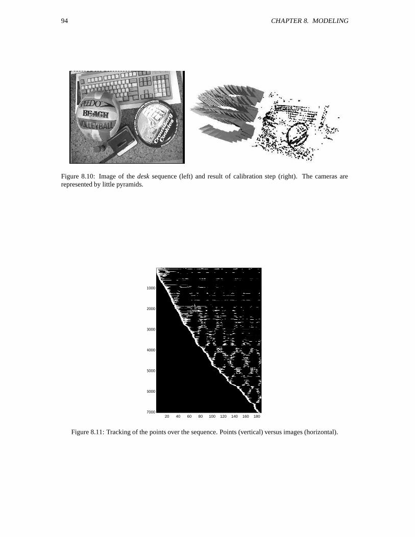
94 CHAPTER 8. MODELING
Figure 8.10: Image of the desk sequence (left) and result of calibration step (right). The cameras arerepresented by little pyramids.
20 40 60 80 100 120 140 160 180
1000
2000
3000
4000
5000
6000
7000
Figure 8.11: Tracking of the points over the sequence. Points (vertical) versus images (horizontal).
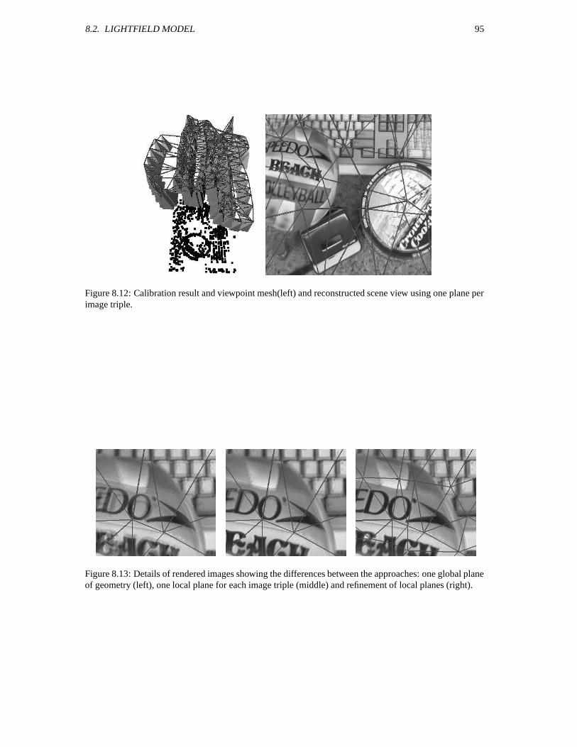
8.2. LIGHTFIELD MODEL 95
Figure 8.12: Calibration result and viewpoint mesh(left) and reconstructed scene view using one plane perimage triple.
Figure 8.13: Details of rendered images showing the differences between the approaches: one global planeof geometry (left), one local plane for each image triple (middle) and refinement of local planes (right).
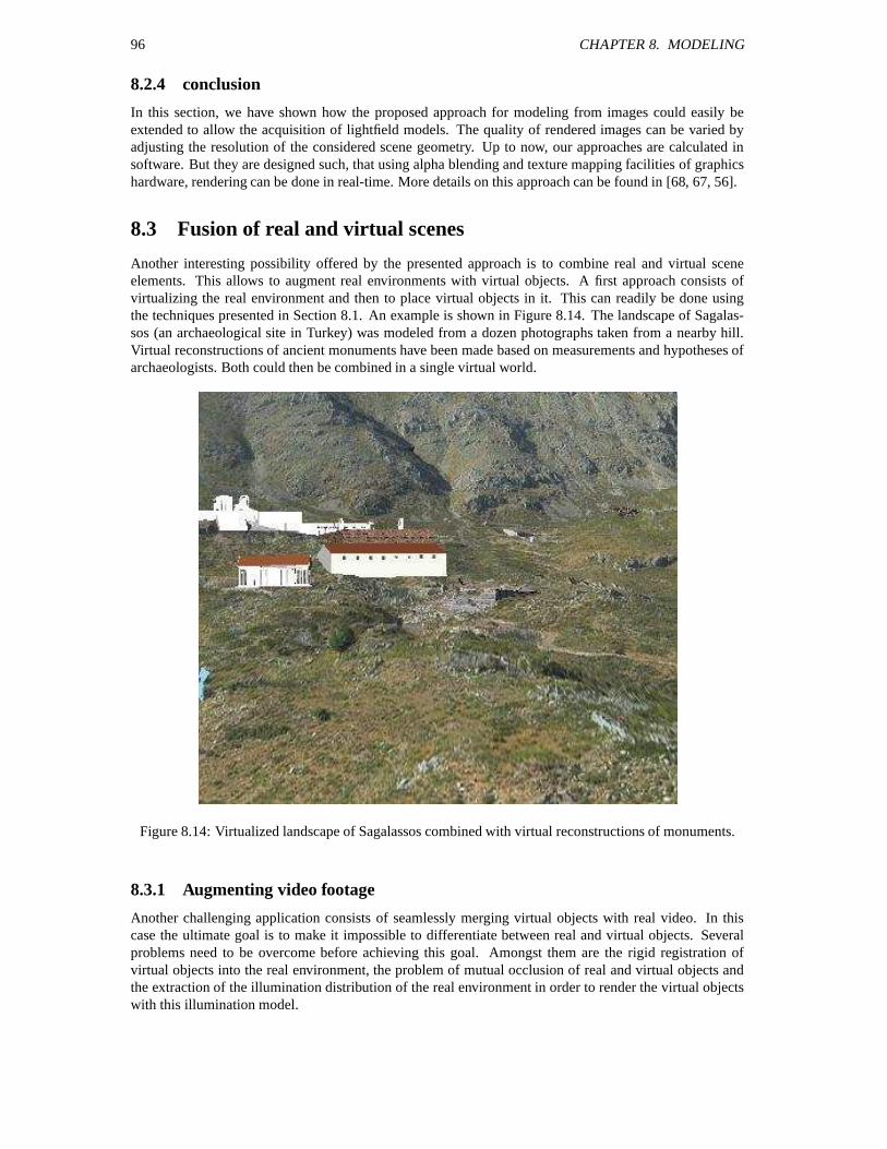
96 CHAPTER 8. MODELING
8.2.4 conclusion
In this section, we have shown how the proposed approach for modeling from images could easily beextended to allow the acquisition of lightfield models. The quality of rendered images can be varied byadjusting the resolution of the considered scene geometry. Up to now, our approaches are calculated insoftware. But they are designed such, that using alpha blending and texture mapping facilities of graphicshardware, rendering can be done in real-time. More details on this approach can be found in [68, 67, 56].
8.3 Fusion of real and virtual scenes
Another interesting possibility offered by the presented approach is to combine real and virtual sceneelements. This allows to augment real environments with virtual objects. A first approach consists ofvirtualizing the real environment and then to place virtual objects in it. This can readily be done usingthe techniques presented in Section 8.1. An example is shown in Figure 8.14. The landscape of Sagalas-sos (an archaeological site in Turkey) was modeled from a dozen photographs taken from a nearby hill.Virtual reconstructions of ancient monuments have been made based on measurements and hypotheses ofarchaeologists. Both could then be combined in a single virtual world.
Figure 8.14: Virtualized landscape of Sagalassos combined with virtual reconstructions of monuments.
8.3.1 Augmenting video footage
Another challenging application consists of seamlessly merging virtual objects with real video. In thiscase the ultimate goal is to make it impossible to differentiate between real and virtual objects. Severalproblems need to be overcome before achieving this goal. Amongst them are the rigid registration ofvirtual objects into the real environment, the problem of mutual occlusion of real and virtual objects andthe extraction of the illumination distribution of the real environment in order to render the virtual objectswith this illumination model.
8.4. CONCLUSION 97
Here we will concentrate on the first of these problems, although the computations described in theprevious section also provide most of the necessary information to solve for occlusions and other inter-actions between the real and virtual components of the augmented scene. Accurate registration of virtualobjects into a real environment is still a challenging problems. Systems that fail to do so will fail to givethe user a real-life impression of the augmented outcome. Since our approach does not use markers ora-priori knowledge of the scene or the camera, this allows us to deal with video footage of unpreparedenvironments or archive video footage. More details on this approach can be found in [14].
An important difference with the applications discussed in the previous sections is that in this case allframes of the input video sequence have to be processed while for 3D modeling often a sparse set of viewsis sufficient. Therefore, in this case features should be tracked from frame to frame. As already mentionedin Section 5.1 it is important that the structure is initialized from frames that are sufficiently separated.Another key component is the bundle adjustment. It does not only reduce the frame to frame jitter, butremoves the largest part of the error that the structure and motion approach accumulates over the sequence.According to our experience it is very important to extend the perspective camera model with at least oneparameter for radial distortion to obtain an undistorted metric structure (this will be clearly demonstratedin the example). Undistorted models are required to position larger virtual entities correctly in the modeland to avoid drift of virtual objects in the augmented video sequences. Note however that for the renderingof the virtual objects the computed radial distortion can most often be ignored (except for sequences whereradial distortion is immediately noticeable from single images).
examples A first set of experiments was carried out on video sequences of the Beguinage in Leuven(the same as in Figure 9.7). The sequence was recorded with a digital camcorder in progressive-scanmode to avoid interlacing problems. Once the structure and motion has been computed, the next stepconsists of positioning the virtual objects with respect to the real scene. This process is illustrated inFigure 8.15. The virtual objects are positioned within the computed 3D structure. To allow a precisepositioning, feedback is immediately given by rendering the virtual object in some selected key-frames.After satisfactory placement of each single virtual object the computed camera corresponding to eachimage is used to render the virtual objects on top of the video. Anti-aliasing can be obtained by mergingmultiple views of the virtual objects obtained with a small offset on the principal point. Some frames ofthe Beguinage video sequence augmented with a cube are also shown in Figure 8.15.
Another example was recorded at Sagalassos in Turkey, where the footage of the ruins of an ancientfountain was taken. The fountain video sequence consists of 250 frames. A large part of the original mon-ument is missing. Based on results of archaeological excavations and architectural studies, it was possibleto generate a virtual copy of the missing part. Using the proposed approach the virtual reconstruction couldbe placed back on the remains of the original monument, at least in the recorded video sequence. Thismaterial is of great interest to the archaeologists, not only for education and dissemination, but also forfund raising to achieve a real restoration of the fountain. The top part of Figure 8.16 shows a top view ofthe recovered structure before and after bundle-adjustment. Besides the larger reconstruction error it canalso be noticed that the non-refined structure is slightly bent. This effect mostly comes from not taking theradial distortion into account in the initial structure recovery. Therefore, a bundle adjustment that did notmodel radial distortion would not yield satisfying results. In the rest of Figure 8.16 some frames of theaugmented video are shown.
8.4 Conclusion
In this chapter different methods were proposed to obtain 3D models from data computed as described inthe previous chapters. The flexibility of the approach also allowed us to compute plenoptic models fromimage sequences acquired with a hand-held camera and to develope a flexible augmented reality systemthat can augment video seamlessly.
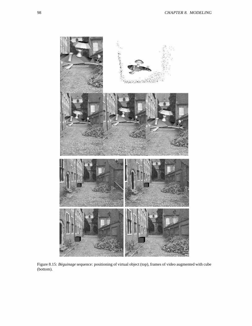
98 CHAPTER 8. MODELING
Figure 8.15: Beguinage sequence: positioning of virtual object (top), frames of video augmented with cube(bottom).
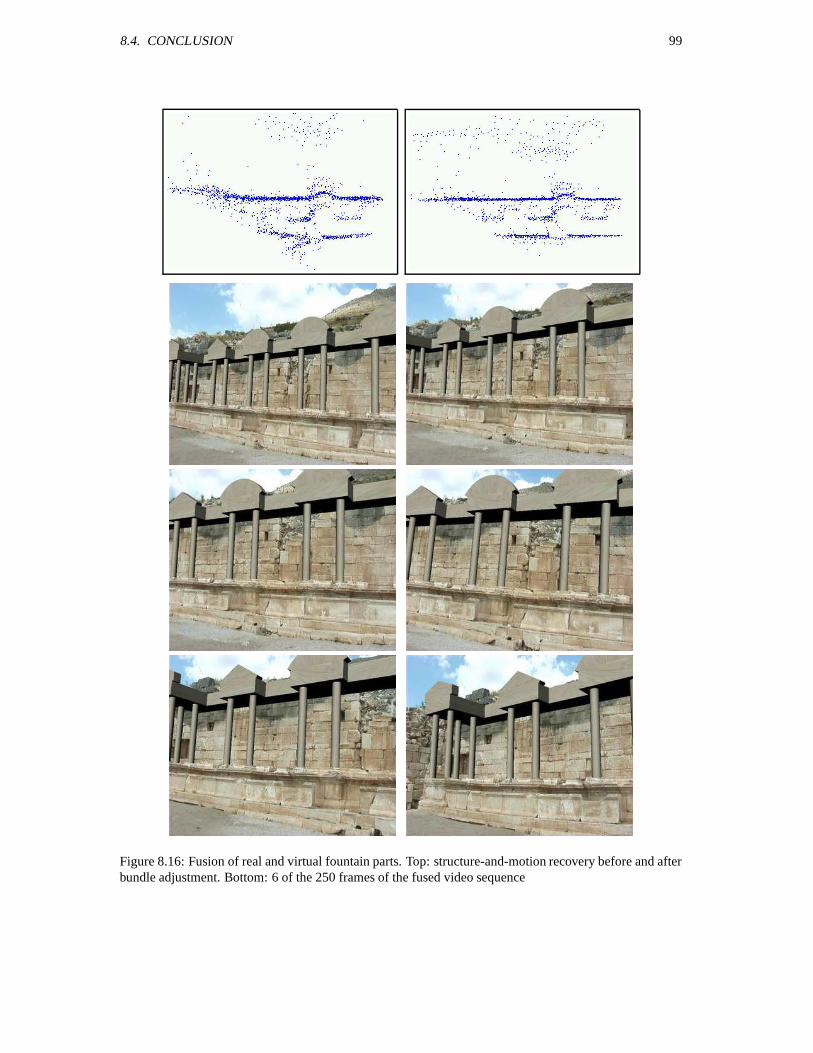
8.4. CONCLUSION 99
Figure 8.16: Fusion of real and virtual fountain parts. Top: structure-and-motion recovery before and afterbundle adjustment. Bottom: 6 of the 250 frames of the fused video sequence

100 CHAPTER 8. MODELING
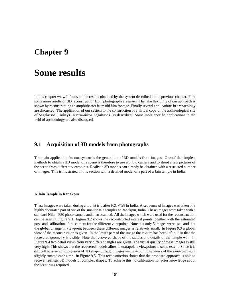
Chapter 9
Some results
In this chapter we will focus on the results obtained by the system described in the previous chapter. Firstsome more results on 3D reconstruction from photographs are given. Then the flexibility of our approach isshown by reconstructing an amphitheater from old film footage. Finally several applications in archaeologyare discussed. The application of our system to the construction of a virtual copy of the archaeological siteof Sagalassos (Turkey) –a virtualized Sagalassos– is described. Some more specific applications in thefield of archaeology are also discussed.
9.1 Acquisition of 3D models from photographs
The main application for our system is the generation of 3D models from images. One of the simplestmethods to obtain a 3D model of a scene is therefore to use a photo camera and to shoot a few pictures ofthe scene from different viewpoints. Realistic 3D models can already be obtained with a restricted numberof images. This is illustrated in this section with a detailed model of a part of a Jain temple in India.
A Jain Temple in Ranakpur
These images were taken during a tourist trip after ICCV’98 in India. A sequence of images was taken of ahighly decorated part of one of the smaller Jain temples at Ranakpur, India. These images were taken with astandard Nikon F50 photo camera and then scanned. All the images which were used for the reconstructioncan be seen in Figure 9.1. Figure 9.2 shows the reconstructed interest points together with the estimatedpose and calibration of the camera for the different viewpoints. Note that only 5 images were used and thatthe global change in viewpoint between these different images is relatively small. In Figure 9.3 a globalview of the reconstruction is given. In the lower part of the image the texture has been left out so that therecovered geometry is visible. Note the recovered shape of the statues and details of the temple wall. InFigure 9.4 two detail views from very different angles are given. The visual quality of these images is stillvery high. This shows that the recovered models allow to extrapolate viewpoints to some extent. Since it isdifficult to give an impression of 3D shape through images we have put three views of the same part –butslightly rotated each time– in Figure 9.5. This reconstruction shows that the proposed approach is able torecover realistic 3D models of complex shapes. To achieve this no calibration nor prior knowledge aboutthe scene was required.
101
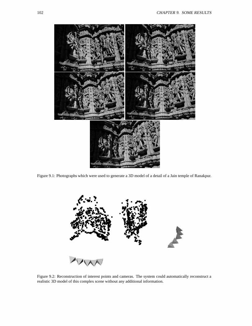
102 CHAPTER 9. SOME RESULTS
Figure 9.1: Photographs which were used to generate a 3D model of a detail of a Jain temple of Ranakpur.
Figure 9.2: Reconstruction of interest points and cameras. The system could automatically reconstruct arealistic 3D model of this complex scene without any additional information.
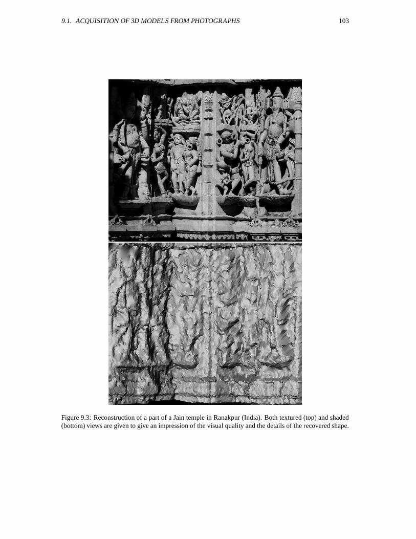
9.1. ACQUISITION OF 3D MODELS FROM PHOTOGRAPHS 103
Figure 9.3: Reconstruction of a part of a Jain temple in Ranakpur (India). Both textured (top) and shaded(bottom) views are given to give an impression of the visual quality and the details of the recovered shape.
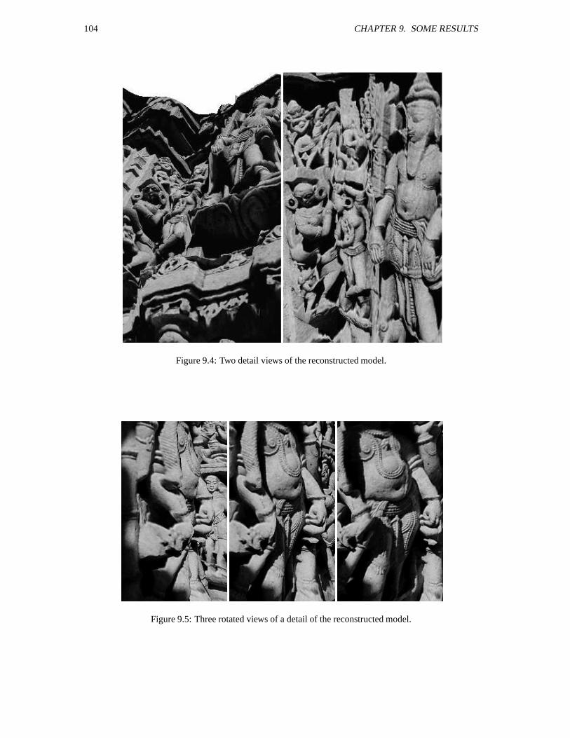
104 CHAPTER 9. SOME RESULTS
Figure 9.4: Two detail views of the reconstructed model.
Figure 9.5: Three rotated views of a detail of the reconstructed model.
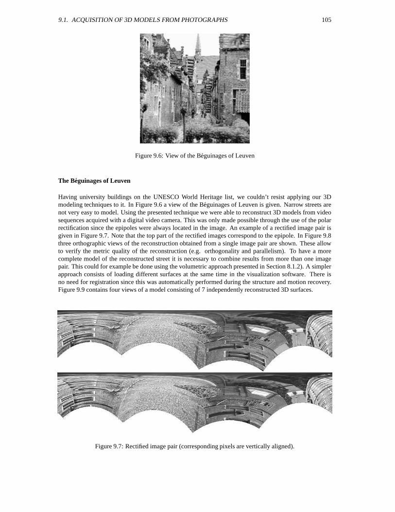
9.1. ACQUISITION OF 3D MODELS FROM PHOTOGRAPHS 105
Figure 9.6: View of the Beguinages of Leuven
The Beguinages of Leuven
Having university buildings on the UNESCO World Heritage list, we couldn’t resist applying our 3Dmodeling techniques to it. In Figure 9.6 a view of the Beguinages of Leuven is given. Narrow streets arenot very easy to model. Using the presented technique we were able to reconstruct 3D models from videosequences acquired with a digital video camera. This was only made possible through the use of the polarrectification since the epipoles were always located in the image. An example of a rectified image pair isgiven in Figure 9.7. Note that the top part of the rectified images correspond to the epipole. In Figure 9.8three orthographic views of the reconstruction obtained from a single image pair are shown. These allowto verify the metric quality of the reconstruction (e.g. orthogonality and parallelism). To have a morecomplete model of the reconstructed street it is necessary to combine results from more than one imagepair. This could for example be done using the volumetric approach presented in Section 8.1.2). A simplerapproach consists of loading different surfaces at the same time in the visualization software. There isno need for registration since this was automatically performed during the structure and motion recovery.Figure 9.9 contains four views of a model consisting of 7 independently reconstructed 3D surfaces.
Figure 9.7: Rectified image pair (corresponding pixels are vertically aligned).
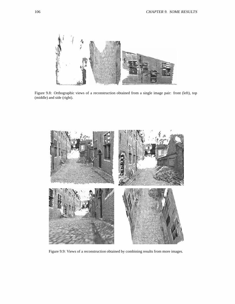
106 CHAPTER 9. SOME RESULTS
Figure 9.8: Orthographic views of a reconstruction obtained from a single image pair: front (left), top(middle) and side (right).
Figure 9.9: Views of a reconstruction obtained by combining results from more images.
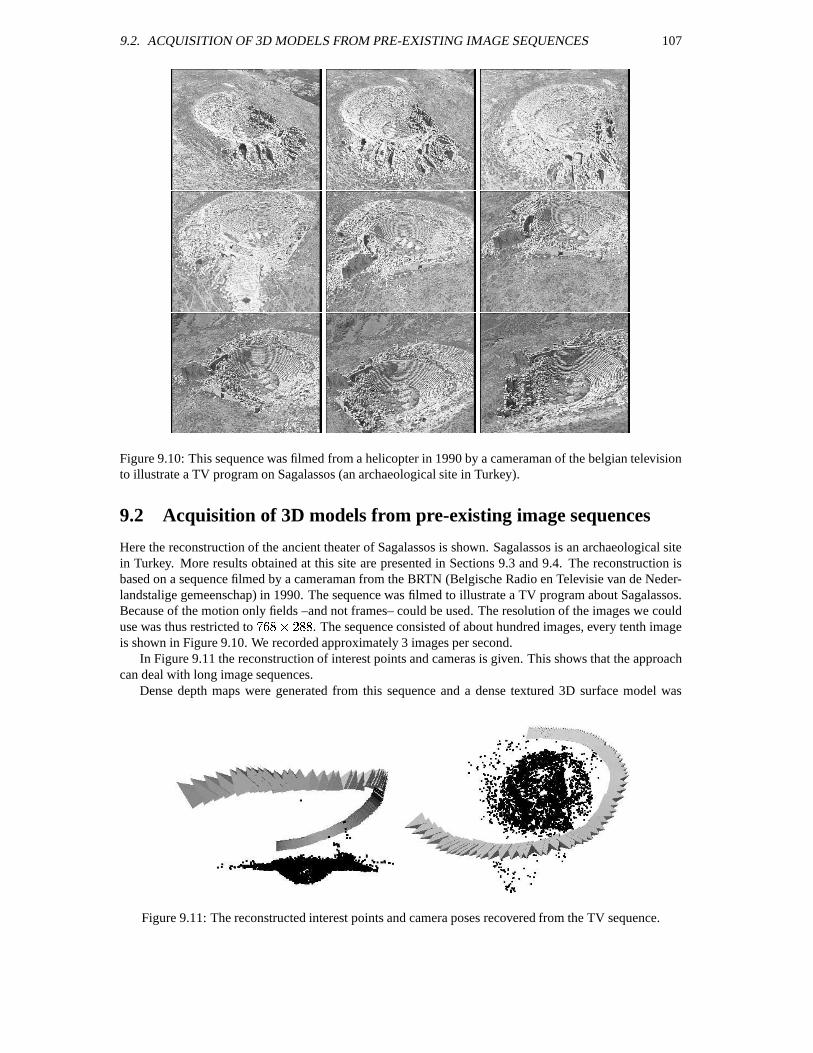
9.2. ACQUISITION OF 3D MODELS FROM PRE-EXISTING IMAGE SEQUENCES 107
Figure 9.10: This sequence was filmed from a helicopter in 1990 by a cameraman of the belgian televisionto illustrate a TV program on Sagalassos (an archaeological site in Turkey).
9.2 Acquisition of 3D models from pre-existing image sequences
Here the reconstruction of the ancient theater of Sagalassos is shown. Sagalassos is an archaeological sitein Turkey. More results obtained at this site are presented in Sections 9.3 and 9.4. The reconstruction isbased on a sequence filmed by a cameraman from the BRTN (Belgische Radio en Televisie van de Neder-landstalige gemeenschap) in 1990. The sequence was filmed to illustrate a TV program about Sagalassos.Because of the motion only fields –and not frames– could be used. The resolution of the images we coulduse was thus restricted to
. The sequence consisted of about hundred images, every tenth imageis shown in Figure 9.10. We recorded approximately 3 images per second.
In Figure 9.11 the reconstruction of interest points and cameras is given. This shows that the approachcan deal with long image sequences.
Dense depth maps were generated from this sequence and a dense textured 3D surface model was
Figure 9.11: The reconstructed interest points and camera poses recovered from the TV sequence.
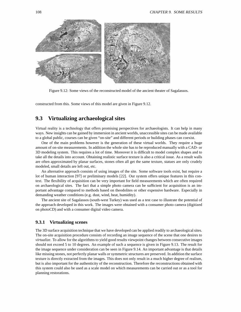
108 CHAPTER 9. SOME RESULTS
Figure 9.12: Some views of the reconstructed model of the ancient theater of Sagalassos.
constructed from this. Some views of this model are given in Figure 9.12.
9.3 Virtualizing archaeological sites
Virtual reality is a technology that offers promising perspectives for archaeologists. It can help in manyways. New insights can be gained by immersion in ancient worlds, unaccessible sites can be made availableto a global public, courses can be given “on-site” and different periods or building phases can coexist.
One of the main problems however is the generation of these virtual worlds. They require a hugeamount of on-site measurements. In addition the whole site has to be reproduced manually with a CAD- or3D modeling system. This requires a lot of time. Moreover it is difficult to model complex shapes and totake all the details into account. Obtaining realistic surface texture is also a critical issue. As a result wallsare often approximated by planar surfaces, stones often all get the same texture, statues are only crudelymodeled, small details are left out, etc.
An alternative approach consists of using images of the site. Some software tools exist, but require alot of human interaction [97] or preliminary models [22]. Our system offers unique features in this con-text. The flexibility of acquisition can be very important for field measurements which are often requiredon archaeological sites. The fact that a simple photo camera can be sufficient for acquisition is an im-portant advantage compared to methods based on theodolites or other expensive hardware. Especially indemanding weather conditions (e.g. dust, wind, heat, humidity).
The ancient site of Sagalassos (south-west Turkey) was used as a test case to illustrate the potential ofthe approach developed in this work. The images were obtained with a consumer photo camera (digitizedon photoCD) and with a consumer digital video camera.
9.3.1 Virtualizing scenes
The 3D surface acquisition technique that we have developed can be applied readily to archaeological sites.The on-site acquisition procedure consists of recording an image sequence of the scene that one desires tovirtualize. To allow for the algorithms to yield good results viewpoint changes between consecutive imagesshould not exceed 5 to 10 degrees. An example of such a sequence is given in Figure 9.13. The result forthe image sequence under consideration can be seen in Figure 9.14. An important advantage is that detailslike missing stones, not perfectly planar walls or symmetric structures are preserved. In addition the surfacetexture is directly extracted from the images. This does not only result in a much higher degree of realism,but is also important for the authenticity of the reconstruction. Therefore the reconstructions obtained withthis system could also be used as a scale model on which measurements can be carried out or as a tool forplanning restorations.
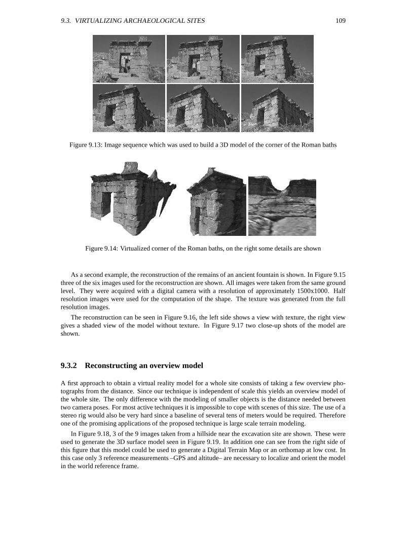
9.3. VIRTUALIZING ARCHAEOLOGICAL SITES 109
Figure 9.13: Image sequence which was used to build a 3D model of the corner of the Roman baths
Figure 9.14: Virtualized corner of the Roman baths, on the right some details are shown
As a second example, the reconstruction of the remains of an ancient fountain is shown. In Figure 9.15three of the six images used for the reconstruction are shown. All images were taken from the same groundlevel. They were acquired with a digital camera with a resolution of approximately 1500x1000. Halfresolution images were used for the computation of the shape. The texture was generated from the fullresolution images.
The reconstruction can be seen in Figure 9.16, the left side shows a view with texture, the right viewgives a shaded view of the model without texture. In Figure 9.17 two close-up shots of the model areshown.
9.3.2 Reconstructing an overview model
A first approach to obtain a virtual reality model for a whole site consists of taking a few overview pho-tographs from the distance. Since our technique is independent of scale this yields an overview model ofthe whole site. The only difference with the modeling of smaller objects is the distance needed betweentwo camera poses. For most active techniques it is impossible to cope with scenes of this size. The use of astereo rig would also be very hard since a baseline of several tens of meters would be required. Thereforeone of the promising applications of the proposed technique is large scale terrain modeling.
In Figure 9.18, 3 of the 9 images taken from a hillside near the excavation site are shown. These wereused to generate the 3D surface model seen in Figure 9.19. In addition one can see from the right side ofthis figure that this model could be used to generate a Digital Terrain Map or an orthomap at low cost. Inthis case only 3 reference measurements –GPS and altitude– are necessary to localize and orient the modelin the world reference frame.
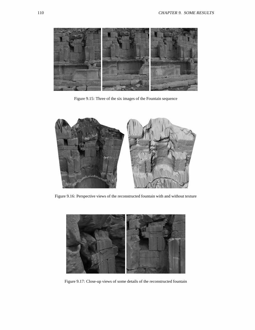
110 CHAPTER 9. SOME RESULTS
Figure 9.15: Three of the six images of the Fountain sequence
Figure 9.16: Perspective views of the reconstructed fountain with and without texture
Figure 9.17: Close-up views of some details of the reconstructed fountain
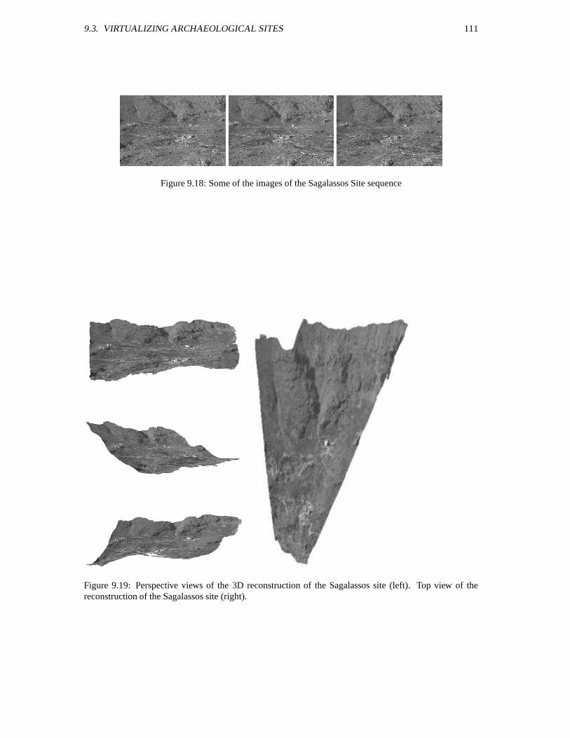
9.3. VIRTUALIZING ARCHAEOLOGICAL SITES 111
Figure 9.18: Some of the images of the Sagalassos Site sequence
Figure 9.19: Perspective views of the 3D reconstruction of the Sagalassos site (left). Top view of thereconstruction of the Sagalassos site (right).
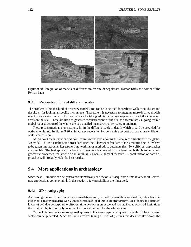
112 CHAPTER 9. SOME RESULTS
Figure 9.20: Integration of models of different scales: site of Sagalassos, Roman baths and corner of theRoman baths.
9.3.3 Reconstructions at different scales
The problem is that this kind of overview model is too coarse to be used for realistic walk-throughs aroundthe site or for looking at specific monuments. Therefore it is necessary to integrate more detailed modelsinto this overview model. This can be done by taking additional image sequences for all the interestingareas on the site. These are used to generate reconstructions of the site at different scales, going from aglobal reconstruction of the whole site to a detailed reconstruction for every monument.
These reconstructions thus naturally fill in the different levels of details which should be provided foroptimal rendering. In Figure 9.20 an integrated reconstruction containing reconstructions at three differentscales can be seen.
At this point the integration was done by interactively positioning the local reconstructions in the global3D model. This is a cumbersome procedure since the 7 degrees of freedom of the similarity ambiguity haveto be taken into account. Researchers are working on methods to automate this. Two different approachesare possible. The first approach is based on matching features which are based on both photometric andgeometric properties, the second on minimizing a global alignment measure. A combination of both ap-proaches will probably yield the best results.
9.4 More applications in archaeology
Since these 3D models can be generated automatically and the on-site acquisition time is very short, severalnew applications come to mind. In this section a few possibilities are illustrated.
9.4.1 3D stratigraphy
Archaeology is one of the sciences were annotations and precise documentation are most important becauseevidence is destroyed during work. An important aspect of this is the stratigraphy. This reflects the differentlayers of soil that correspond to different time periods in an excavated sector. Due to practical limitationsthis stratigraphy is often only recorded for some slices, not for the whole sector.
Our technique allows a more optimal approach. For every layer a complete 3D model of the excavatedsector can be generated. Since this only involves taking a series of pictures this does not slow down the
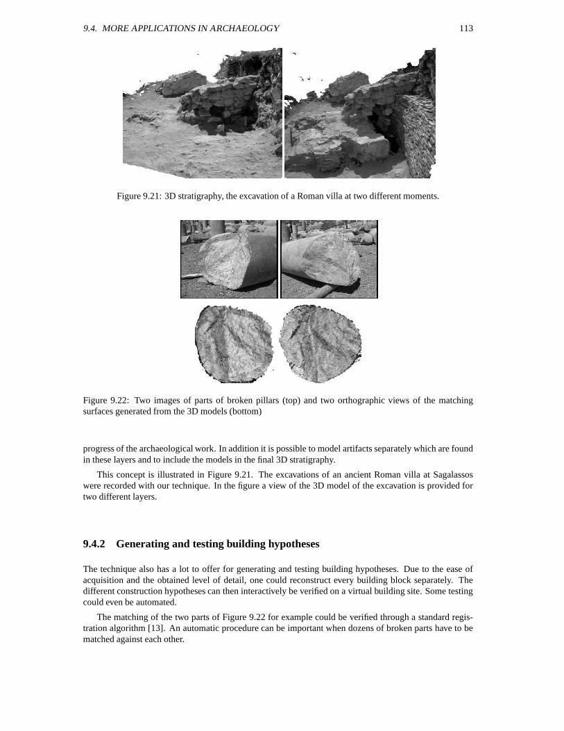
9.4. MORE APPLICATIONS IN ARCHAEOLOGY 113
Figure 9.21: 3D stratigraphy, the excavation of a Roman villa at two different moments.
Figure 9.22: Two images of parts of broken pillars (top) and two orthographic views of the matchingsurfaces generated from the 3D models (bottom)
progress of the archaeological work. In addition it is possible to model artifacts separately which are foundin these layers and to include the models in the final 3D stratigraphy.
This concept is illustrated in Figure 9.21. The excavations of an ancient Roman villa at Sagalassoswere recorded with our technique. In the figure a view of the 3D model of the excavation is provided fortwo different layers.
9.4.2 Generating and testing building hypotheses
The technique also has a lot to offer for generating and testing building hypotheses. Due to the ease ofacquisition and the obtained level of detail, one could reconstruct every building block separately. Thedifferent construction hypotheses can then interactively be verified on a virtual building site. Some testingcould even be automated.
The matching of the two parts of Figure 9.22 for example could be verified through a standard regis-tration algorithm [13]. An automatic procedure can be important when dozens of broken parts have to bematched against each other.
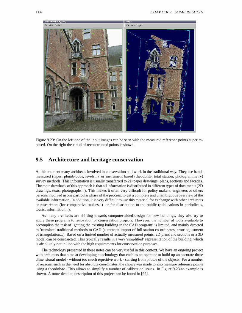
114 CHAPTER 9. SOME RESULTS
Figure 9.23: On the left one of the input images can be seen with the measured reference points superim-posed. On the right the cloud of reconstructed points is shown.
9.5 Architecture and heritage conservation
At this moment many architects involved in conservation still work in the traditional way. They use hand-measured (tapes, plumb-bobs, levels...) or instrument based (theodolite, total station, photogrammetry)survey methods. This information is usually transferred to 2D paper drawings: plans, sections and facades.The main drawback of this approach is that all information is distributed in different types of documents (2Ddrawings, texts, photographs...). This makes it often very difficult for policy makers, engineers or otherspersons involved in one particular phase of the process, to get a complete and unambiguous overview of theavailable information. In addition, it is very difficult to use this material for exchange with other architectsor researchers (for comparative studies...) or for distribution to the public (publications in periodicals,tourist information...).
As many architects are shifting towards computer-aided design for new buildings, they also try toapply these programs to renovation or conservation projects. However, the number of tools available toaccomplish the task of ’getting the existing building in the CAD program’ is limited, and mainly directedto ’translate’ traditional methods to CAD (automatic import of full station co-ordinates, error-adjustmentof triangulation...). Based on a limited number of actually measured points, 2D plans and sections or a 3Dmodel can be constructed. This typically results in a very ’simplified’ representation of the building, whichis absolutely not in line with the high requirements for conservation purposes.
The technology presented in these notes can be very useful in this context. We have an ongoing projectwith architects that aims at developing a technology that enables an operator to build up an accurate threedimensional model - without too much repetitive work - starting from photos of the objects. For a numberof reasons, such as the need for absolute coordinates, the choice was made to also measure reference pointsusing a theodolyte. This allows to simplify a number of calibration issues. In Figure 9.23 an example isshown. A more detailed description of this project can be found in [92].
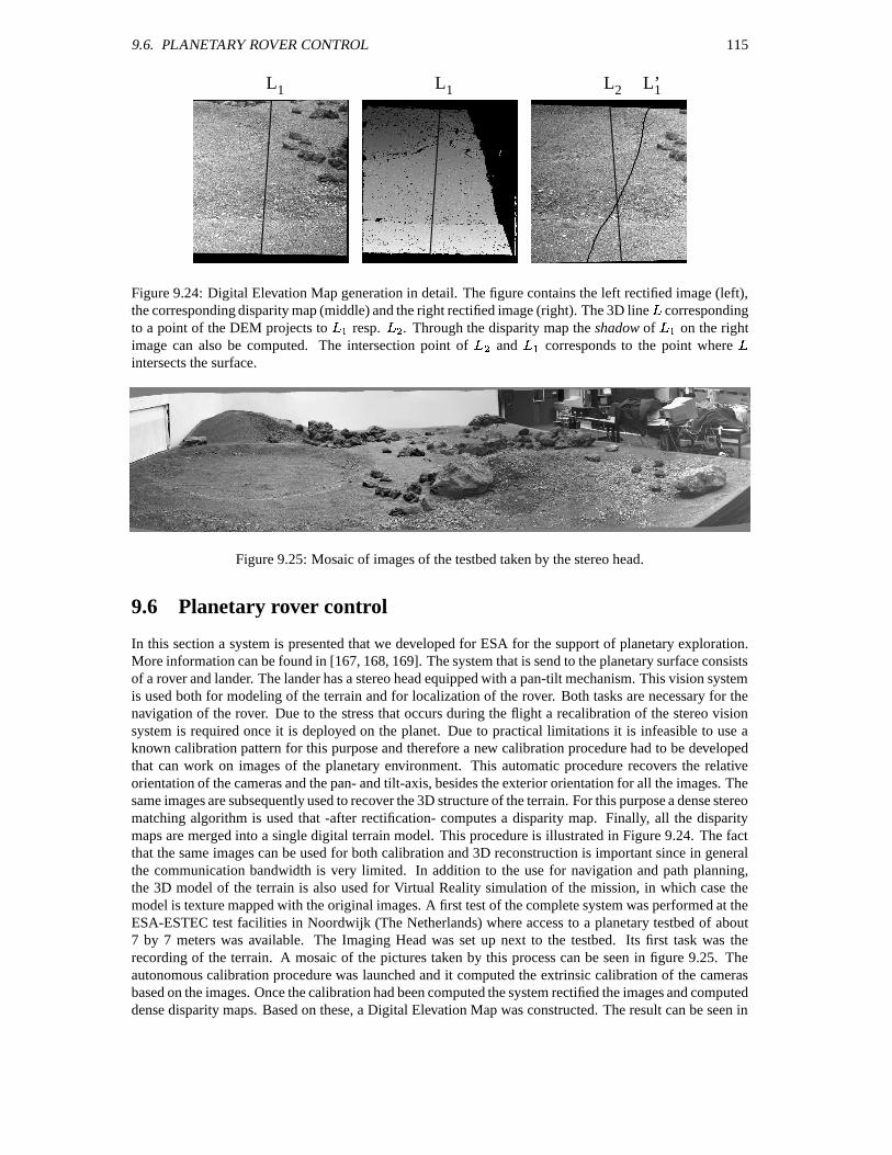
9.6. PLANETARY ROVER CONTROL 115
L L L L’1 1 2 1
Figure 9.24: Digital Elevation Map generation in detail. The figure contains the left rectified image (left),the corresponding disparity map (middle) and the right rectified image (right). The 3D line correspondingto a point of the DEM projects to W resp. , . Through the disparity map the shadow of W on the rightimage can also be computed. The intersection point of , and W corresponds to the point where intersects the surface.
Figure 9.25: Mosaic of images of the testbed taken by the stereo head.
9.6 Planetary rover control
In this section a system is presented that we developed for ESA for the support of planetary exploration.More information can be found in [167, 168, 169]. The system that is send to the planetary surface consistsof a rover and lander. The lander has a stereo head equipped with a pan-tilt mechanism. This vision systemis used both for modeling of the terrain and for localization of the rover. Both tasks are necessary for thenavigation of the rover. Due to the stress that occurs during the flight a recalibration of the stereo visionsystem is required once it is deployed on the planet. Due to practical limitations it is infeasible to use aknown calibration pattern for this purpose and therefore a new calibration procedure had to be developedthat can work on images of the planetary environment. This automatic procedure recovers the relativeorientation of the cameras and the pan- and tilt-axis, besides the exterior orientation for all the images. Thesame images are subsequently used to recover the 3D structure of the terrain. For this purpose a dense stereomatching algorithm is used that -after rectification- computes a disparity map. Finally, all the disparitymaps are merged into a single digital terrain model. This procedure is illustrated in Figure 9.24. The factthat the same images can be used for both calibration and 3D reconstruction is important since in generalthe communication bandwidth is very limited. In addition to the use for navigation and path planning,the 3D model of the terrain is also used for Virtual Reality simulation of the mission, in which case themodel is texture mapped with the original images. A first test of the complete system was performed at theESA-ESTEC test facilities in Noordwijk (The Netherlands) where access to a planetary testbed of about7 by 7 meters was available. The Imaging Head was set up next to the testbed. Its first task was therecording of the terrain. A mosaic of the pictures taken by this process can be seen in figure 9.25. Theautonomous calibration procedure was launched and it computed the extrinsic calibration of the camerasbased on the images. Once the calibration had been computed the system rectified the images and computeddense disparity maps. Based on these, a Digital Elevation Map was constructed. The result can be seen in
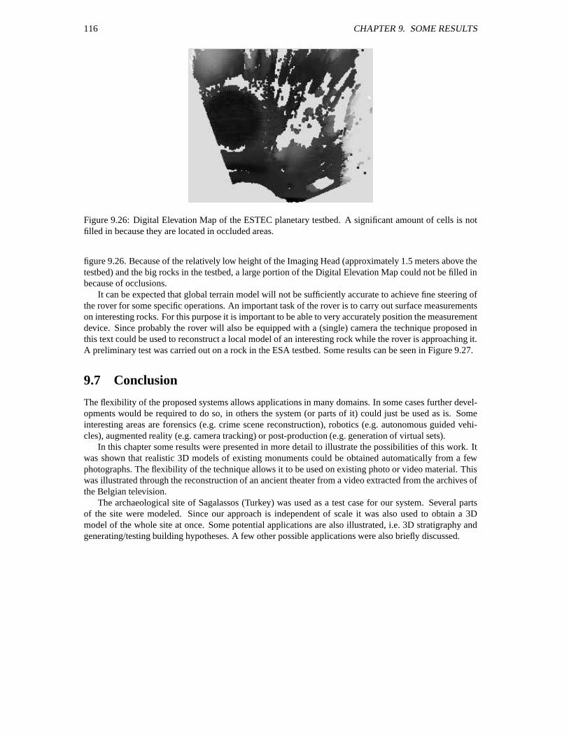
116 CHAPTER 9. SOME RESULTS
Figure 9.26: Digital Elevation Map of the ESTEC planetary testbed. A significant amount of cells is notfilled in because they are located in occluded areas.
figure 9.26. Because of the relatively low height of the Imaging Head (approximately 1.5 meters above thetestbed) and the big rocks in the testbed, a large portion of the Digital Elevation Map could not be filled inbecause of occlusions.
It can be expected that global terrain model will not be sufficiently accurate to achieve fine steering ofthe rover for some specific operations. An important task of the rover is to carry out surface measurementson interesting rocks. For this purpose it is important to be able to very accurately position the measurementdevice. Since probably the rover will also be equipped with a (single) camera the technique proposed inthis text could be used to reconstruct a local model of an interesting rock while the rover is approaching it.A preliminary test was carried out on a rock in the ESA testbed. Some results can be seen in Figure 9.27.
9.7 Conclusion
The flexibility of the proposed systems allows applications in many domains. In some cases further devel-opments would be required to do so, in others the system (or parts of it) could just be used as is. Someinteresting areas are forensics (e.g. crime scene reconstruction), robotics (e.g. autonomous guided vehi-cles), augmented reality (e.g. camera tracking) or post-production (e.g. generation of virtual sets).
In this chapter some results were presented in more detail to illustrate the possibilities of this work. Itwas shown that realistic 3D models of existing monuments could be obtained automatically from a fewphotographs. The flexibility of the technique allows it to be used on existing photo or video material. Thiswas illustrated through the reconstruction of an ancient theater from a video extracted from the archives ofthe Belgian television.
The archaeological site of Sagalassos (Turkey) was used as a test case for our system. Several partsof the site were modeled. Since our approach is independent of scale it was also used to obtain a 3Dmodel of the whole site at once. Some potential applications are also illustrated, i.e. 3D stratigraphy andgenerating/testing building hypotheses. A few other possible applications were also briefly discussed.
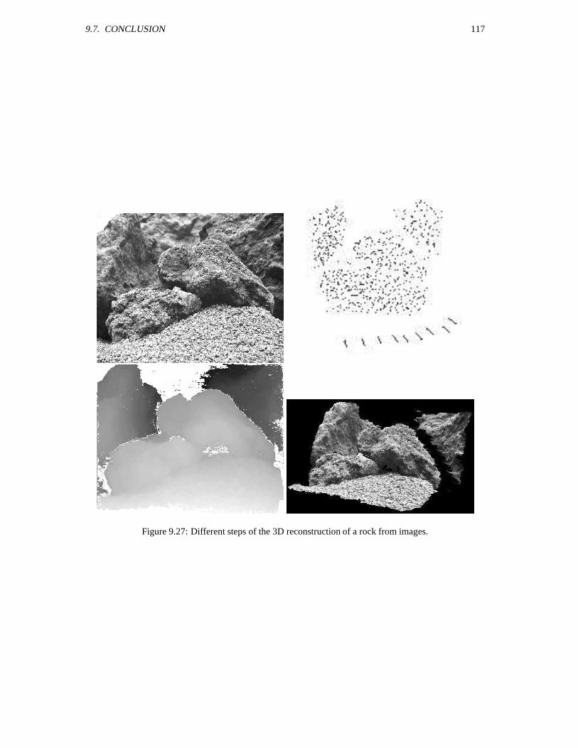
9.7. CONCLUSION 117
Figure 9.27: Different steps of the 3D reconstruction of a rock from images.

118 CHAPTER 9. SOME RESULTS
Appendix A
Bundle adjustment
Once the structure and motion has been obtained for the whole sequence, it is recommended to refine itthrough a global minimization step. A maximum likelihood estimation can be obtained through bundleadjustment [12, 137]. The goal is to find the projection matrices
and the 3D points
for which themean squared distances between the observed image points and the reprojected image points
isminimized. For views and , points the following criterion should be minimized:
>L M W
.L M WYN P , (A.1)
whereYN P is the Euclidean image distance. If the image error is zero-mean Gaussian then bundle
adjustment is the Maximum Likelihood Estimator. Although it can be expressed very simply, this mini-mization problem is huge. For a typical sequence of 20 views and 2000 points, a minimization problem inmore than 6000 variables has to be solved. A straight-forward computation is obviously not feasible. How-ever, the special structure of the problem can be exploited to solve the problem much more efficiently. Theobserved points being fixed, a specific residual
& YN P , is only dependent on the point -th point and the -th camera view. This results in a sparse structure for the normal equations. Using thisstructure the points
can be eliminated from the equations, yielding a much smaller but denser problem.
Views that have features in common are now related. For a long sequence where features tend to only beseen in a few consecutive views, the matrix that has to be solved is still sparse (typically band diagonal).In this vcase it can be very interesting to make use of sparse linear algebra algorithms, e.g. [3].
Before going more into detail on efficiently solving the bundle adjustment, the Levenberg-Marquardtminimization is presented. Based one this an efficient method for bundle adjustment will be proposed inSection A.2.
A.1 Levenberg-Marquardt minimization
Given a vector relation 7 & N 0 P where 0 and 7 can have different dimensions and an observation7 , we
want to find the vector 0 which best satisfies the given relation. More precisely, we are looking for thevector
0 satisfying78& N 0 P . for which
H H is minimal.
A.1.1 Newton iteration
Newton’s approach starts from an initial value 0 and refines this value using the assumption that islocally linear. A first order approximation of N 0 . P yields:
N 0 . P & N 0 P . (A.2)
with
the Jacobian matrix and
a small displacement. Under these assumptions minimizing &
can be solved through linear least-squares. A simple derivation yields S & S (A.3)
119
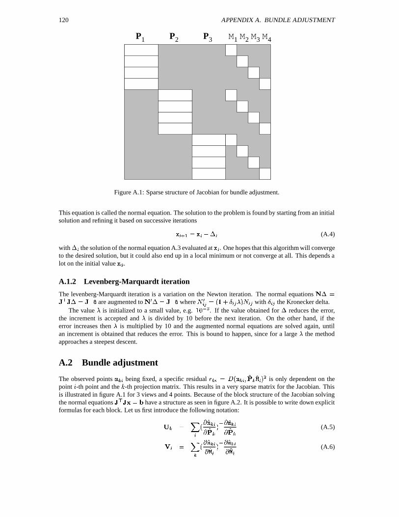
120 APPENDIX A. BUNDLE ADJUSTMENT
P P P M M M M1 3 41 2 3 2
Figure A.1: Sparse structure of Jacobian for bundle adjustment.
This equation is called the normal equation. The solution to the problem is found by starting from an initialsolution and refining it based on successive iterations
0 4 W & 0 . (A.4)
with
the solution of the normal equation A.3 evaluated at 0 . One hopes that this algorithm will convergeto the desired solution, but it could also end up in a local minimum or not converge at all. This depends alot on the initial value 0 .A.1.2 Levenberg-Marquardt iteration
The levenberg-Marquardt iteration is a variation on the Newton iteration. The normal equations & S & S are augmented to E & S where EL & N . L A P L with L the Kronecker delta.
The value A is initialized to a small value, e.g. ( U . If the value obtained for
reduces the error,the increment is accepted and A is divided by 10 before the next iteration. On the other hand, if theerror increases then A is multiplied by 10 and the augmented normal equations are solved again, untilan increment is obtained that reduces the error. This is bound to happen, since for a large A the methodapproaches a steepest descent.
A.2 Bundle adjustment
The observed points being fixed, a specific residual & YN P , is only dependent on the
point -th point and the -th projection matrix. This results in a very sparse matrix for the Jacobian. Thisis illustrated in figure A.1 for 3 views and 4 points. Because of the block structure of the Jacobian solvingthe normal equations
S & have a structure as seen in figure A.2. It is possible to write down explicitformulas for each block. Let us first introduce the following notation:
& L N
P S (A.5)
& LN
P S (A.6)
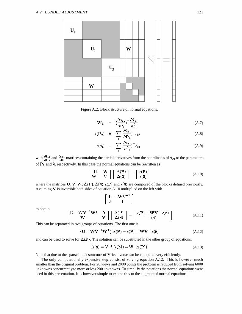
A.2. BUNDLE ADJUSTMENT 121
U
U
U
W
W2
1
3
Figure A.2: Block structure of normal equations.
& N
P S (A.7)
N P & L N
P S (A.8)
N P & L N
P S (A.9)
with and
matrices containing the partial derivatives from the coordinates of to the parameters
of and respectively. In this case the normal equations can be rewritten as
S N PTN P & N P N P (A.10)
where the matrices TN P TN P N P and N P are composed of the blocks defined previously.Assuming is invertible both sides of equation A.10 multiplied on the left with \
UXW \
to obtain UZW S
S N PN P & N P UXW N P
N P (A.11)
This can be separated in two groups of equations. The first one is
UZW S N P & N P UXW N P (A.12)
and can be used to solve forN P
. The solution can be substituted in the other group of equations:N P & UZW N P S TN P (A.13)
Note that due to the sparse block structure of its inverse can be computed very efficiently.The only computationally expensive step consist of solving equation A.12. This is however much
smaller than the original problem. For 20 views and 2000 points the problem is reduced from solving 6000unknowns concurrently to more or less 200 unknowns. To simplify the notations the normal equations wereused in this presentation. It is however simple to extend this to the augmented normal equations.

122 APPENDIX A. BUNDLE ADJUSTMENT
Bibliography
[1] H. Akaike, “A new look at the statistical model identification”, IEEE Trans. on Automatic Control,19-6, pp 716-723, 1974.
[2] M. Armstrong, A. Zisserman and R. Hartley, “Euclidean Reconstruction from Image Triplets”, Com-puter Vision - ECCV’96, Lecture Notes in Computer Science, Vol. 1064, Springer-Verlag, pp. 3-16,1996.
[3] C. Ashcraft and R. Grimes. “SPOOLES: An object-oriented sparse matrix library”. In Proceedingsof the 9th SIAM Conference on Parallel Processing for Scientific Computing, San-Antonio, Texas,1999. 10 pages on CD-ROM.
[4] N. Ayache and C. Hansen, “Rectification of images for binocular and trinocular stereovision”, Proc.Intern. Conf. on Pattern Recognition, pp. 11-16, 1988.
[5] A. Azerbayejani, B. Horowitz and A. Pentland, “Recursive estimation of structure from motion usingrelative orientation constraints”, Proceedings of the International Conference of Computer Vision andPattern Recognition, IEEE Computer Society Press, pp.294-299, June 1993.
[6] H. Baker and T. Binford, “Depth from Edge and Intensity Based Stereo”, Int. Joint Conf. on ArtificialIntelligence, Vancouver, Canada, pp. 631-636, 1981.
[7] P. Beardsley, A. Zisserman and D. Murray, “Sequential Updating of Projective and Affine Structurefrom Motion”, International Journal of Computer Vision (23), No. 3, Jun-Jul 1997, pp. 235-259.
[8] D. Bondyfalat and S. Bougnoux, “Imposing Euclidean Constraints During Self-Calibration Pro-cesses”, Proc. SMILE Workshop (post-ECCV’98), Lecture Notes in Computer Science, Vol. 1506,Springer-Verlag, pp.224-235, 1998.
[9] B. Boufama, R. Mohr and F. Veillon, “Euclidian Constraints for Uncalibrated Reconstruction”, Proc.International Conference on Computer Vision, pp. 466-470, 1993.
[10] J.-Y. Bouguet and P. Perona, “3D Photography on your Desk”. Proc. 6th Int. Conf. Computer Vision,Bombay, India, pages 43-50, January 1998.
[11] D. Brown, “Close-range camera calibration”, Photogrammetric Engineering, 37(8):855-866, 1971.
[12] D. Brown, “The bundle adjustment - progress and prospect”, XIII Congress of the ISPRS, Helsinki,1976.
[13] Y. Chen and G. Medioni, “Object Modeling by Registration of Multiple Range Images”, Proc. Int.Conf. on Robotics and Automation, 1991.
[14] K. Cornelis, M. Pollefeys, M. Vergauwen and L. Van Gool, “Augmented Reality from UncalibratedVideo Sequences”, In M. Pollefeys, L. Van Gool, A. Zisserman, A. Fitzgibbon (Eds.), 3D Structurefrom Images - SMILE 2000, Lecture Notes in Computer Science, Vol. 2018, pp.150-167, Springer-Verlag, 2001.
123
124 BIBLIOGRAPHY
[15] P. Courtney, N. Thacker and C. Brown, “A hardware architecture for image rectification and groundplane obstacle detection”, Proc. Intern. Conf. on Pattern Recognition, pp. 23-26, 1992.
[16] I. Cox, S. Hingorani and S. Rao, “A Maximum Likelihood Stereo Algorithm”, Computer Vision andImage Understanding, Vol. 63, No. 3, May 1996.
[17] N. Cui, J. Weng and P. Cohen, “Extended Structure and Motion Analysis from Monocular ImageSequences”, Proc. International Conference on Computer Vision, pp. 222-229, Osaka, Japan, 1990.
[18] B. Curless. Better optical triangulation and volumetric reconstruction of complex models from rangeimages. PhD thesis, Stanford University, 1996.
[19] B. Curless and M. Levoy, “A Volumetric Method for Building Complex Models from Range Images”Proc. SIGGRAPH ’96, 1996.
[20] L. de Agapito, R. Hartley and E. Hayman, “Linear calibration of a rotating and zooming camera”,Proc. CVPR, pp. 15-20, 1999.
[21] R. Deriche and G. Giraudon, “A computational approach for corner and vertex detection”, Interna-tional Journal of Computer Vision, 1(2):167-187, 1993.
[22] P. Debevec, C. Taylor and J. Malik, “Modeling and Rendering Architecture from Photographs: AHybrid Geometry- and Image-Based Approach”, Siggraph, 1996.
[23] P. Debevec, Y. Yu and G. Borshukov, “Efficient View-Dependent Image-Based Rendering with Pro-jective Texture Mapping”, Proc. SIGGRAPH ’98, ACM Press, New York, 1998.
[24] U. Dhond and J. Aggarwal, “Structure from Stereo - A Review”, IEEE Trans. Syst., Man and Cybern.19, 1489-1510, 1989.
[25] L. Falkenhagen, “Depth Estimation from Stereoscopic Image Pairs assuming Piecewise ContinuousSurfaces”, European Workshop on Combined Real and Synthetic Image Processing for Broadcast andVideo Productions, Hamburg, Germany, 1994.
[26] L. Falkenhagen, “Hierarchical Block-Based Disparity Estimation Considering Neighbourhood Con-straints”. Proc. International Workshop on SNHC and 3D Imaging, Rhodes, Greece, 1997.
[27] O. Faugeras and G. Toscani, “Camera Calibration for 3D Computer Vision”, International Workshopon Machine Vision and Machine Intelligence, pp. 240-247, Tokyo, 1987.
[28] O. Faugeras, L. Quan and P. Sturm, “Self-Calibration of a 1D Projective Camera and Its Application tothe Self-Calibration of a 2D Projective Camera”, Computer Vision – ECCV’98, vol.1, Lecture Notesin Computer Science, Vol. 1406, Springer-Verlag, pp.36-52, 1998.
[29] O. Faugeras, Three-Dimensional Computer Vision: a Geometric Viewpoint, MIT press, 1993.
[30] O. Faugeras, “Stratification of three-dimensional vision: projective, affine, and metric representa-tions”, Journal of the Optical Society of America A, pp. 465–483, Vol. 12, No.3, March 1995.
[31] O. Faugeras, “What can be seen in three dimensions with an uncalibrated stereo rig”, Computer Vision- ECCV’92, Lecture Notes in Computer Science, Vol. 588, Springer-Verlag, pp. 563-578, 1992.
[32] O. Faugeras, Q.-T. Luong and S. Maybank. “Camera self-calibration: Theory and experiments”, Com-puter Vision - ECCV’92, Lecture Notes in Computer Science, Vol. 588, Springer-Verlag, pp. 321-334,1992.
[33] O. Faugeras and S. Maybank, “Motion from point matches: multiplicity of solutions”, InternationalJournal of Computer Vision, 4(3):225-246, June 1990.
[34] O. Faugeras and B. Mourrain, “on the geometry and algebra of point and line correspondences be-tween n images”, Proc. International Conference on Computer Vision, 1995, pp. 951-962.
BIBLIOGRAPHY 125
[35] M. Fischler and R. Bolles, “RANdom SAmpling Consensus: a paradigm for model fitting with ap-plication to image analysis and automated cartography”, Commun. Assoc. Comp. Mach., 24:381-95,1981.
[36] A. Fitzgibbon and A. Zisserman, “Automatic camera recovery for closed or open image sequences”,Computer Vision – ECCV’98, vol.1, Lecture Notes in Computer Science, Vol. 1406, Springer-Verlag,1998. pp.311-326, 1998.
[37] W. Forstner, “A framework for low level feature extraction” Computer Vision-ECCV’90, LectureNotes in Computer Science, Vol. 427, Springer-Verlag, pp.383-394, 1990.
[38] G. Gimel’farb, “Symmetrical approach to the problem of automatic stereoscopic measurements inphotogrammetry”, Cybernetics, 1979, 15(20, 235-247; Consultants Bureau, N.Y.
[39] S. Gortler, R. Grzeszczuk, R. Szeliski and M. F. Cohen, “The Lumigraph”, Proc. SIGGRAPH ’96, pp43–54, ACM Press, New York, 1996.
[40] W. Grimson, From Images to Surfaces: A Computational Study of the Human Early Visual System,MIT Press, Cambridge, Massachusetts, 1981.
[41] A. Gruen, “Accuracy, reliability and statistics in close-range photogrammmetry”, Proceedings of theSymposium of the ISP Commision V, Stockholm, 1978.
[42] A. Gruen and H. Beyer, “System calibration through self-calibration”, Proceedings of the Workshopon Calibration and Orientation of Cameras in Computer Vision, 1992.
[43] G. Golub and C. Van Loan, Matrix Computations, John Hopkins University Press, 1983.
[44] R. Haralick, C. Lee, K. Ottenberg, and M. Nolle, “Review and Analysis of Solutions of the ThreePoint Perspective Pose Estimation Problem”, International Journal of Computer Vision, Vol.13, No.3,1994, pp. 331-356.
[45] C. Harris and M. Stephens, “A combined corner and edge detector”, Fourth Alvey Vision Conference,pp.147-151, 1988.
[46] R. Hartley, “Estimation of relative camera positions for uncalibrated cameras”, Computer Vision -ECCV’92, Lecture Notes in Computer Science, Vol. 588, Springer-Verlag, pp. 579-587, 1992.
[47] R.Hartley, Chirality International Journal of Computer Vision, 26(1):41-61, January 1998.
[48] R. Hartley, “Euclidean reconstruction from uncalibrated views”, in : J.L. Mundy, A. Zisserman, andD. Forsyth (eds.), Applications of Invariance in Computer Vision, Lecture Notes in Computer Science,Vol. 825, Springer-Verlag, pp. 237-256, 1994.
[49] R. Hartley, “Projective reconstruction from line correspondences”, Proc. IEEE Conference on Com-puter Vision and Pattern Recognition, IEEE Computer Society Press, 1994.
[50] R. Hartley, “Self-calibration from multiple views with a rotating camera”, Lecture Notes in ComputerScience, Vol. 800-801, Springer-Verlag, pp. 471-478, 1994.
[51] R. Hartley, “A linear method for reconstruction from points and lines”, Proc. International Conferenceon Computer Vision, pp. 882-887, 1995.
[52] R. Hartley, “In defense of the eight-point algorithm”. IEEE Trans. on Pattern Analysis and MachineIntelligence, 19(6):580-593, June 1997.
[53] R. Hartley and P. Sturm, “Triangulation”, Computer Vision and Image Understanding, 68(2):146-157,1997.
[54] R. Hartley, “Computation of the Quadrifocal Tensor”, Computer Vision-ECCV’98, Lecture Notes inComputer Science, Vol. 1406, Springer-Verlag, pp. 20-35, 1998.
126 BIBLIOGRAPHY
[55] R. Hartley and A. Zisserman, Multiple View Geometry in Computer Vision, Cambridge UniversityPress, 2000.
[56] B. Heigl, R. Koch, M. Pollefeys, J. Denzler and L. Van Gool, “Plenoptic Modeling and Renderingfrom Image Sequences taken by Hand-held Camera”, In Proc. DAGM’99, pp.94-101.
[57] A. Heyden and K. Astrom, “Euclidean Reconstruction from Constant Intrinsic Parameters” Proc. 13thInternational Conference on Pattern Recognition, IEEE Computer Soc. Press, pp. 339-343, 1996.
[58] A. Heyden and K. Astrom, “Euclidean Reconstruction from Image Sequences with Varying and Un-known Focal Length and Principal Point”, Proc. IEEE Conference on Computer Vision and PatternRecognition, IEEE Computer Soc. Press, pp. 438-443, 1997.
[59] A. Heyden, Geometry and Algebra of Multiple Projective Transformations, Ph.D.thesis, Lund Uni-versity, 1995.
[60] A. Heyden and K. Astrom, “Minimal Conditions on Intrinsic Parameters for Euclidean Reconstruc-tion”, Asian Conference on Computer Vision, Hong Kong, 1998.
[61] M. Irani and S. Peleg, Super resolution from image sequences, Proc. International Conference onPattern Recognition, Atlantic City, NJ, 1990.
[62] F. Kahl, “Critical Motions and Ambiuous Euclidean Reconstructions in Auto-Calibration”, Proc.ICCV, pp.469-475, 1999.
[63] F. Kahl, B. Triggs, K. strm, “Critical Motions for Auto-Calibration When Some Intrinsic ParametersCan Vary”, Journal of Mathematical Imaging and Vision 13,131-146,2000.
[64] K. Kanatani, Statistical Optimization for Geometric Computation: Theory and Practice , ElsevierScience, Amsterdam, 1996.
[65] W. Karl, G. Verghese and A. Willsky, Reconstructing ellipsoids from projections. CVGIP; GraphicalModels and Image Processing, 56(2):124-139, 1994.
[66] R. Koch, M. Pollefeys, L. Van Gool, “Realistic surface reconstruction of 3D scenes from uncalibratedimage sequences”, Journal Visualization and Computer Animation, Vol. 11, pp. 115-127, 2000.
[67] R. Koch, M. Pollefeys, B. Heigl, L. Van Gool and H. Niemann. “Calibration of Hand-held CameraSequences for Plenoptic Modeling”, Proc.ICCV’99 (international Conference on Computer Vision),pp.585-591, Corfu (Greece), 1999.
[68] R. Koch, B. Heigl, M. Pollefeys, L. Van Gool and H. Niemann, “A Geometric Approach to LightfieldCalibration”, Proc. CAIP99, LNCS 1689, Springer-Verlag, pp.596-603, 1999.
[69] R. Koch, Automatische Oberflachenmodellierung starrer dreidimensionaler Objekte aus stereoskopis-chen Rundum-Ansichten, PhD thesis, University of Hannover, Germany, 1996 also published asFortschritte-Berichte VDI, Reihe 10, Nr.499, VDI Verlag, 1997.
[70] R. Koch, M. Pollefeys and L. Van Gool, Multi Viewpoint Stereo from Uncalibrated Video Sequences.Proc. European Conference on Computer Vision, pp.55-71. Freiburg, Germany, 1998.
[71] R. Koch, M. Pollefeys and L. Van Gool, Automatic 3D Model Acquisition from Uncalibrated ImageSequences, Proceedings Computer Graphics International, pp.597-604, Hannover, 1998.
[72] R. Koch: Surface Segmentation and Modeling of 3-D Polygonal Objects from Stereoscopic ImagePairs. Proc. ICPR’96, Vienna 1996.
[73] R. Koch, “3-D Surface Reconstruction from Stereoscopic Image Sequences”, Proc. Fifth Interna-tional Conference on Computer Vision, IEEE Computer Soc. Press, pp. 109-114, 1995.
BIBLIOGRAPHY 127
[74] A. Koschan, “Eine Methodenbank zur Evaluierung von Stereo-Vision-Verfahren”, Ph.D. Thesis,Technische Universitat Berlin, Berlin, Germany, 1991.
[75] E. Kruppa, “Zur ermittlung eines objektes aus zwei perspektiven mit innerer orientierung”, Sitz.-Ber.Akad. Wiss., Wien, math. naturw. Abt. IIa, 122:1939-1948, 1913.
[76] S. Laveau and O. Faugeras, “Oriented Projective Geometry for Computer Vision”, in : B. Buxtonand R. Cipolla (eds.), Computer Vision - ECCV’96, Lecture Notes in Computer Science, Vol. 1064,Springer-Verlag, pp. 147-156, 1996.
[77] R. Lenz and R. Tsai, “Techniques for calibration of the scale factor and image center for high accuracy3-D machine vision metrology”, IEEE Transactions on Pattern Analysis and Machine Intelligence,10:713-720, 1988.
[78] M. Levoy and P. Hanrahan, “Lightfield Rendering”, Proc. SIGGRAPH ’96, pp 31–42, ACM Press,New York, 1996.
[79] D. Liebowitz and A. Zisserman, “Combining Scene and Auto-calibration Constraints”, Proc. ICCV,pp.293-300, 1999.
[80] H. Longuet-Higgins, “A computer algorithm for reconstructing a scene from two projections”, Nature,293:133-135, 1981.
[81] W.E. Lorensen and H. E. Cline. Marching cubes: A high resolution 3D surface construction algorithm.In Computer Graphics (SIGGRAPH ’87 Proceedings), volume 21, pages 163-169, July 1987.
[82] Q.-T. Luong, Matrice Fondamentale et Autocalibration en Vision par Ordinateur, PhD thesis, Uni-versite de Paris-Sud, France, 1992.
[83] Q.-T. Luong and O. Faugeras, “The fundamental matrix: theory, algorithms, and stability analysis”,Internation Journal of Computer Vision, 17(1):43-76, 1996.
[84] Q.-T. Luong and O. Faugeras, “Self Calibration of a moving camera from point correspondences andfundamental matrices”, Internation Journal of Computer Vision, vol.22-3, 1997.
[85] Y. Ma, S. Soatto, J, Kosecka and S. Sastry, “Euclidean Reconstruction and Reprojection Up to Sub-groups”, Proc. ICCV, pp.773-780, 1999.
[86] D. Marr and T. Poggio, “A Computational Theory of Human Stereo Vision”, Proc. Royal Society ofLondon, Vol. 204 of B, pp. 301-328, 1979.
[87] L. McMillan and G. Bishop, “Plenoptic modeling: An image-based rendering system”, Proc. SIG-GRAPH’95, pp. 39-46, 1995.
[88] T. Moons, “A Guided Tour Through Multiview Relations”, Proc. SMILE Workshop (post-ECCV’98),Lecture Notes in Computer Science 1506, Springer-Verlag, pp.304-346, 1998.
[89] T, Moons, L. Van Gool, M. Proesmans and E. Pauwels, “Affine reconstruction from perspective imagepairs with a relative object-camera translation in between”, IEEE Transactions on Pattern Analysisand Machine Intelligence, vol. 18, no.1, pp. 77-83, Jan. 1996.
[90] H.P. Moravec. “Visual mapping by a robot rover”. Proc. of the 6th International Joint Conference onArtificial Intelligence, pp.598-600, 1979.
[91] J. Mundy and A. Zisserman, “Machine Vision”, in : J.L. Mundy, A. Zisserman, and D. Forsyth(eds.), Applications of Invariance in Computer Vision, Lecture Notes in Computer Science, Vol. 825,Springer-Verlag, 1994.
[92] K. Nuyts, J.P.Kruth, B. Lauwers, M. Pollefeys, L. Qiongyan, J. Schouteden, P. Smars, K. Van Balen,L. Van Gool, M. Vergauwen. “Vision on Conservation: VIRTERF” Proc. International Symposiumon Virtual and Augmented Architecture (VAA01), LNCS, 2001 (in press).
128 BIBLIOGRAPHY
[93] E. Ofek, E. Shilat, A. Rappopport and M. Werman, “Highlight and Reflection Independent Multires-olution Textures from Image Sequences”, IEEE Computer Graphics and Applications, vol.17 (2),March-April 1997.
[94] Y. Ohta and T. Kanade, “Stereo by Intra- and Inter-scanline Search Using Dynamic Programming”,IEEE Trans. on Pattern Analysis and Machine Intelligence 7(2), 139-154, 1985.
[95] M. Okutomi and T. Kanade, “A Locally Adaptive Window for Signal Processing”, International Jour-nal of Computer Vision, 7, 143-162, 1992.
[96] D. Papadimitriou and T. Dennis, “Epipolar line estimation and rectification for stereo image pairs”,IEEE Trans. Image Processing, 5(4):672-676, 1996.
[97] PhotoModeler, by Eos Systems Inc., http://www.photomodeler.com/.
[98] S. Pollard, J. Mayhew and J. Frisby, “PMF: A Stereo Correspondence Algorithm Using a DisparityGradient Limit”, Perception 14(4), 449-470, 1985.
[99] M. Pollefeys, Self-calibration and metric 3D reconstruction from uncalibrated image sequences, PhD.thesis, K.U.Leuven, 1999.
[100] M. Pollefeys, F. Verbiest, L. Van Gool, “Surviving dominant planes in uncalibrated structure andmotion recovery”, Proc. ECCV 2002, LNCS.
[101] M. Pollefeys, R. Koch, M. Vergauwen, L. Van Gool. “Automated reconstruction of 3D scenes fromsequences of images”, Isprs Journal Of Photogrammetry And Remote Sensing (55)4 (2000), pp. 251-267.
[102] M. Pollefeys, M. Vergauwen, L. Van Gool, “Automatic 3D modeling from image sequences”, In-ternational Archive of Photogrammetry and Remote Sensing, Vol. XXXIII, Part B5, pp. 619-626,2000.
[103] M. Pollefeys, R. Koch, M. Vergauwen, B. Deknuydt, L. Van Gool. “Three-dimensional scene re-construction from images”, proc. SPIE Electronic Imaging, Three-Dimensional Image Capture andApplications III, SPIE Proceedings series Vol. 3958, pp.215-226, 2000.
[104] M. Pollefeys and L. Van Gool, “Stratified self-calibration with the modulus constraint”, accepted forpublication in IEEE transactions on Pattern Analysis and Machine Intelligence.
[105] M. Pollefeys, R. Koch and L. Van Gool. “Self-Calibration and Metric Reconstruction in spite ofVarying and Unknown Internal Camera Parameters”, International Journal of Computer Vision.
[106] M. Pollefeys, R. Koch and L. Van Gool, ”A simple and efficient rectification method for generalmotion”, Proc.ICCV’99 (international Conference on Computer Vision), pp.496-501, Corfu (Greece),1999.
[107] M. Pollefeys, R. Koch, M. Vergauwen and L. Van Gool, “An Automatic Method for Acquiring3D models from Photographs: applications to an Archaeological Site”, accepted for Proc. ISPRSInternational Workshop on Photogrammetric Measurements, Object Modeling and Documentation inArchitecture and Industry, july 1999.
[108] M. Pollefeys, M. Proesmans, R. Koch, M. Vergauwen and L. Van Gool, “Detailed model acquisitionfor virtual reality”, in J. Barcelo, M. Forte and D. Sanders (eds.), Virtual Reality in Archaeology, toappear, ArcheoPress, Oxford.
[109] M. Pollefeys, R. Koch, M. Vergauwen and L. Van Gool, “Automatic Generation of 3D Models fromPhotographs”, Proceedings Virtual Systems and MultiMedia, 1998.
[110] M. Pollefeys, R. Koch, M. Vergauwen and L. Van Gool, “Virtualizing Archaeological Sites”, Pro-ceedings Virtual Systems and MultiMedia, 1998.
BIBLIOGRAPHY 129
[111] M. Pollefeys, R. Koch, M. Vergauwen and L. Van Gool, “Metric 3D Surface Reconstruction fromUncalibrated Image Sequences”, Proc. SMILE Workshop (post-ECCV’98), Lecture Notes in Com-puter Science, Vol. 1506, pp.138-153, Springer-Verlag, 1998.
[112] M. Pollefeys, R. Koch, M. Vergauwen and L. Van Gool, “Flexible acquisition of 3D structure frommotion”, Proceedings IEEE workshop on Image and Multidimensional Digital Signal Processing,pp.195-198, Alpbach, 1998.
[113] M. Pollefeys, R. Koch, M. Vergauwen and L. Van Gool, “Flexible 3D Acquisition with a MonocularCamera”, Proceedings IEEE International Conference on Robotics and Automation, Vol.4, pp.2771-2776, Leuven, 1998.
[114] M. Pollefeys, R. Koch and L. Van Gool, “Self-Calibration and Metric Reconstruction in spite ofVarying and Unknown Internal Camera Parameters”, Proc. International Conference on ComputerVision, Narosa Publishing House, pp.90-95, 1998.
[115] M. Pollefeys, L. Van Gool and M. Proesmans, “Euclidean 3D Reconstruction from Image Sequenceswith Variable Focal Lengths”, Computer Vision - ECCV’96, Lecture Notes in Computer Science,Vol. 1064, Springer-Verlag, pp. 31-42, 1996.
[116] M. Pollefeys, L. Van Gool and A. Oosterlinck, “The Modulus Constraint: A New Constraint forSelf-Calibration”, Proc. 13th International Conference on Pattern Recognition, IEEE Computer Soc.Press, pp. 349-353, 1996.
[117] M. Pollefeys and L. Van Gool, “A stratified approach to self-calibration”, Proc. 1997 Conference onComputer Vision and Pattern Recognition, IEEE Computer Soc. Press, pp. 407-412, 1997.
[118] M. Pollefeys and L. Van Gool, “Self-calibration from the absolute conic on the plane at infinity”,Proc. Computer Analysis of Images and Patterns, Lecture Notes in Computer Science, Vol. 1296,Springer-Verlag, pp. 175-182, 1997.
[119] M. Pollefeys, L. Van Gool and T. Moons. “Euclidean 3D reconstruction from stereo sequences withvariable focal lengths”, Recent Developments in Computer Vision, Lecture Notes in Computer Sci-ence, Vol.1035, Springer-Verlag, pp. 405-414, 1996.
[120] M. Pollefeys, L. Van Gool and T. Moons. “Euclidean 3D reconstruction from stereo sequences withvariable focal lengths”, Proc.Asian Conference on Computer Vision, Vol.2, pp.6-10, Singapore, 1995
[121] M. Pollefeys, L. Van Gool and A. Oosterlinck, “Euclidean self-calibration via the modulus con-straint”, in F.Dillen, L.Vrancken, L.Verstraelen, and I. Van de Woestijne (eds.), Geometry and topol-ogy of submanifolds, VIII, World Scientific, Singapore, New Jersey, London, Hong Kong, pp.283-291,1997.
[122] W. Press, S. Teukolsky and W. Vetterling, Numerical recipes in C: the art of scientific computing,Cambridge university press, 1992.
[123] P. Pritchett and A. Zisserman, “Wide Baseline Stereo Matching”, Proc. International Conference onComputer Vision, Narosa Publishing House, pp. 754-760, 1998.
[124] P. Pritchett and A. Zisserman, “Matching and Reconstruction from Widely Separate Views”, Proc.SMILE Workshop (post-ECCV’98), Lecture Notes in Computer Science, Vol. 1506, Springer-Verlag,pp.78-92, 1998.
[125] M. Proesmans, L. Van Gool and A. Oosterlinck, “Determination of optical flow and its discontinu-ities using non-linear diffusion”, Computer Vision - ECCV’94, Lecture Notes in Computer Science,Vol. 801, Springer-Verlag, pp. 295-304, 1994.
[126] M. Proesmans, L. Van Gool, F. Defoort, “Reading between the lines - a method for extracting dy-namic 3D with texture”, Sixth international conference on computer vision, pp. 1081-1086, January4-7, 1998.

130 BIBLIOGRAPHY
[127] P. Rousseeuw, Robust Regression and Outlier Detection, Wiley, New York, 1987.
[128] S. Roy, J. Meunier and I. Cox, “Cylindrical Rectification to Minimize Epipolar Distortion”, Proc.IEEE Conference on Computer Vision and Pattern Recognition, pp.393-399, 1997.
[129] F. Schaffalitzky and A. Zisserman, “Geometric Grouping of Repeated Elements within Images”,Proc. 9th British Machine Vision Conference, pp 13-22, 1998.
[130] C. Schmid and R. Mohr, “Local Greyvalue Invariants for Image Retrieval”, IEEE transactions onPattern Analysis and Machine Intelligence, Vol.19, no.5, pp 872-877, may 1997.
[131] C. Schmid, R. Mohr and C. Bauckhage, “Comparing and Evaluating Interest Points”, Proc. Interna-tional Conference on Computer Vision, Narosa Publishing House, pp. 230-235, 1998.
[132] J.G. Semple and G.T. Kneebone, Algebraic Projective Geometry, Oxford University Press, 1952.
[133] ShapeSnatcher, by Eyetronics, http://www.eyetronics.com/.
[134] A. Shashua, “Omni-Rig Sensors: What Can be Done With a Non-Rigid Vision Platform?” Proc. ofthe Workshop on Applications of Computer Vision (WACV), Princeton, Oct. 1998.
[135] A. Shashua, “Trilinearity in visual recognition by alignment”, Computer Vision - ECCV’94, LectureNotes in Computer Science, Vol. 801, Springer-Verlag, pp. 479-484, 1994.
[136] J. Shi and C. Tomasi, “Good Features to Track”, Proc. IEEE Conference on Computer Vision andPattern Recognition (CVPR’94), pp. 593 - 600, 1994.
[137] C. Slama, Manual of Photogrammetry, American Society of Photogrammetry, Falls Church, VA,USA, 4th edition, 1980.
[138] M. Soucy and D. Laurendeau. “A general surface approach to the integration of a set of range views”.IEEE Transactions on Pattern Analysis and Machine Intelligence, 17(4):344-358, April 1995.
[139] S.M. Smith and J.M. Brady. “SUSAN - a new approach to low level image processing”. Int. Journalof Computer Vision, Vol.23, Nr.1, pp.45-78, 1997.
[140] M. Spetsakis and J. Aloimonos, “Structure from motion using line correspondences”, InternationalJournal of Computer Vision, 4(3):171-183, 1990.
[141] G. Stein, “Lens Distortion Calibration Using Point Correspondences”, Proc. IEEE Conference onComputer Vision and Pattern Recognition, IEEE Computer Soc. Press, pp 602-608, 1997.
[142] P. Sturm, Vision 3D non-calibree: contributions a la reconstruction projective et etudes des mouve-ments critiques pour l’auto-calibrage, Ph.D. Thesis, INP de Grenoble, France , 1997.
[143] P. Sturm and L. Quang, “Affine stereo calibration”, Proceedings Computer Analysis of Images andPatterns, Lecture Notes in Computer Science, Vol. 970, Springer-Verlag, pp. 838-843, 1995.
[144] P. Sturm, “Critical Motion Sequences for Monocular Self-Calibration and Uncalibrated EuclideanReconstruction”, Proc. 1997 Conference on Computer Vision and Pattern Recognition, IEEE Com-puter Soc. Press, pp. 1100-1105, 1997.
[145] P. Sturm, “Critical motion sequences and conjugacy of ambiguous Euclidean reconstructions”, Proc.SCIA - 10th Scandinavian Conference on Image Analysis, Lappeenranta, Finland, pp. 439-446, 1997.
[146] P. Sturm, “Critical Motion Sequences for the Self-Calibration of Cameras and Stereo Systems withVariable Focal Length”. Proc. BMVC - 10th British Machine Vision Conference, pp. 63-72, 1999.
[147] R. Szeliski and S. B. Kang, “Recovering 3D shape and motion from image streams using non-linearleast-squares”, Journal of Visual Communication and Image Representation, 5(1):10–28, March1994.
BIBLIOGRAPHY 131
[148] C. Taylor, P. Debevec and J. Malik, “Reconstructing Polyhedral Models of Architectural Scenesfrom Photographs”, Computer Vision - ECCV’96, Lecture Notes in Computer Science, Vol. 1065,vol.II, pp 659-668, 1996.
[149] C. Tomasi and T. Kanade, “Shape and motion from image streams under orthography: A factoriza-tion approach”, International Journal of Computer Vision, 9(2):137-154, 1992.
[150] P. Torr. “An assessment of information criteria for motion model selection”. In CVPR97, pages 47–53, 1997.
[151] P. Torr and A. Zisserman, “Robust parametrization and computation of the trifocal tensor”, Imageand Vision Computing, 15(1997) 591-605.
[152] P. Torr and A. Zisserman, “Robust Computation and Parameterization of Multiple View Relations”,Proc. International Conference on Computer Vision,Narosa Publishing house, pp 727-732, 1998.
[153] P. Torr, P. Beardsley and D. Murray, “Robust Vision”, Proc. British Machine Vision Conference,1994.
[154] P. Torr, Motion Segmentation and Outlier Detection, PhD Thesis, Dept. of Engineering Science,University of Oxford, 1995.
[155] P. Torr, A. Fitzgibbon and A. Zisserman, “Maintaining Multiple Motion Model Hypotheses OverMany Views to Recover Matching and Structure”, Proc. International Conference on Computer Vi-sion, Narosa Publishing house, pp 485-491, 1998.
[156] B. Triggs, “The geometry of projective reconstruction I: Matching constraints and the joint image”,Proc. International Conference on Computer Vision, IEEE Computer Soc. Press, pp. 338-343, 1995.
[157] B. Triggs, “The Absolute Quadric”, Proc. 1997 Conference on Computer Vision and Pattern Recog-nition, IEEE Computer Soc. Press, pp. 609-614, 1997.
[158] B. Triggs, P. McLauchlan, R. Hartley, A. Fiztgibbon, “Bundle Adjustment – A Modern Synthe-sis”, In B. Triggs, A. Zisserman, R. Szeliski (Eds.), Vision Algorithms: Theory and Practice, LNCSVol.1883, pp.298-372, Springer-Verlag, 2000.
[159] R. Tsai and T. Huang, “Uniqueness and Estimation of Three-Dimensional Motion Parameters ofRigid Objects with Curved Surfaces”, IEEE transactions on Pattern Analysis and Machine Intelli-gence, vol.6, pp.13-27, Jan. 1984.
[160] R. Tsai, “An efficient and accurate camera calibration technique for 3D machine vision”, Proc.Computer Vision and Pattern Recognition, 1986.
[161] R. Tsai. “A versatile camera calibration technique for high-accuracy 3D machine vision using off-the-shelf TV cameras and lenses”. IEEE Journal of Robotics and Automation, RA-3(4):323-331,August 1987.
[162] G. Turk and M. Levoy ”Zippered Polygon Meshes from Range Images” Proceedings of SIGGRAPH’94 pp. 311-318.
[163] T. Tuytelaars. M. Vergauwen, M. Pollefeys and L. Van Gool, ”Image Matching for Wide baselineStereo”, Proc. International Conference on Forensic Human Identification, 1999.
[164] T. Tuytelaars and L. Van Gool ”Wide Baseline Stereo based on Local, Affinely invariant Regions”British Machine Vision Conference, pp. 412-422, 2000.
[165] L. Van Gool, F. Defoort, R. Koch, M. Pollefeys, M. Proesmans and M. Vergauwen, “3D modelingfor communications”, Proceedings Computer Graphics International, pp.482-487, Hannover, 1998.
132 BIBLIOGRAPHY
[166] L. Van Gool, T. Moons, D. Ungureanu, “Affine/photometric invariants for planar intensity patterns”, Proceedings 4th European Conference on Computer Vision, ECCV’96, Lecture Notes in ComputerScience, vol. 1064, pp.642-651, 1996.
[167] M. Vergauwen, M. Pollefeys, L. Van Gool, “A stereo vision system for support of planetary surfaceexploration”, Proc. International Conference on Vision Systems, LNCS, 2001.
[168] M. Vergauwen, M. Pollefeys, R. Moreas, F. Xu, G. Visentin, L. Van Gool and H. Van Brussel.“Calibration, Terrain Reconstruction and Path Planning for a Planetary Exploration System”, Proc.i-SAIRAS 2001.
[169] M. Vergauwen, M. Pollefeys, L. Van Gool, Calibration and 3D measurements from Martian TerrainImages, Proc. International Conference on Robotics and Automation, IEEE Computer Society Press,2001.
[170] J. Weng, P. Cohen and M. Herniou, “Camera calibration with distortion models and accuracy evalu-ation”, IEEE Transaction on Pattern Analysis and Machine Intelligence, 14(10):965-980, 1992.
[171] R. Willson and S. Shafer, “A Perspective Projection Camera Model for Zoom Lenses”, ProceedingsSecond Conference on Optical 3-D Measurement Techniques, Zurich Switzerland, October 1993.
[172] R. Willson, “Modeling and Calibration of Automated Zoom Lenses” Proceedings of the SPIE2350:Videometrics III, Boston MA, October 1994, pp.170-186.
[173] R. Willson, Modeling and Calibration of Automated Zoom Lenses, Ph.D. thesis, Department ofElectrical and Computer Engineering, Carnegie Mellon University, January 1994.
[174] R. Willson and S. Shafer, “What is the Center of the Image?”, Journal of the Optical Society ofAmerica A, Vol. 11, No. 11, pp.2946-2955, November 1994.
[175] G. Wolberg, Digital Image Warping, IEEE Computer Society Press Monograph, ISBN 0-8186-8944-7, 1990.
[176] C. Zeller, Calibration projective, affine et Euclidienne en vision par ordinateur et application a laperception tridimensionnelle, Ph.D. Thesis, Ecole Polytechnique, France, 1996.
[177] Z. Zhang, R. Deriche, O. Faugeras and Q.-T. Luong, “A robust technique for matching two un-calibrated images through the recovery of the unknown epipolar geometry”, Artificial IntelligenceJournal, Vol.78, pp.87-119, October 1995.
[178] Z. Zhang, “On the Epipolar Geometry Between Two Images with Lens Distortion”, Proc. Interna-tional Conference on Pattern Recognition, IEEE Computer Soc. Press, A80.13, 1996.
[179] C. Loop and Z. Zhang. “Computing Rectifying Homographies for Stereo Vision”. IEEE Conf. Com-puter Vision and Pattern Recognition (CVPR’99), Colorado, June 1999.
[180] A. Zisserman, D. Liebowitz and M. Armstrong, “Resolving ambiguities in auto-calibration”, Phil.Trans. R. Soc. Lond., A(1998) 356, 1193-1211.
Curriculum Vitae
Marc Pollefeys is an assistant professor at the computer science department of the University of NorthCarolina – Chapel Hill since July 2002. Before this he was a post-doctoral researcher of the Funds for Sci-entific Research - Flanders affiliated to the Center for Processing of Speech and Images of the K.U.Leuven.His PhD dissertation on ”Self-calibration and Metric 3D Reconstruction from Uncalibrated Image Se-quences” was awarded the Scientific Prize BARCO 1999. His current research focuses on 3D modelingfrom images, multi-view geometry, image-based rendering, virtual and augmented reality and applications.He is currently involved in projects ranging from digital archaeology, over immersive video and 3D tele-vision, to planetary rover control. Marc Pollefeys has published over 60 technical papers and won severalawards, amongst which the prestigious Marr Prize at the International Conference on Computer Visionin 1998. He is the chair of the working group on Image Sequences of the International Society for Pho-togrammetry and Remote Sensing (ISPRS). He has organized the Second European Workshop on Structurefrom Multiple Images of Large-scale Environments in Dublin in 2000 and several courses and tutorials atmajor vision and graphics conferences. He has served on the program commitee of several internationalconferences and workshops and is a regular reviewer for most major computer vision, computer graphicsand photogrammetry journals and conferences.
133