Embed Size (px)
Citation preview
VIRTUAL TESTING OF ADVANCED POLYMERCOMPOSITE MATERIALS
Ana Andreia Pinheiro Durao Branco
Master’s ThesisAdvisor: Prof. Dr. Pedro Ponces Camanho
Mestrado Integrado em Engenharia Mecanica
July 17, 2015

Abstract
In this thesis, the validation of the models used to virtually predict inelas-tic deformation and fracture of advanced polymer composites is performed.Due to the complex response of the composite materials, a building blockvalidation is followed making the analysis of growing complexity accordingto the specimen used.
Different damage mechanisms, namely matrix transverse cracking, fibrefracture and delamination, are analysed and the CFRP’s response studiedaccordingly, with the help of Abaqus UEL (user subroutines) and VUMATsubroutines. The development of the mesh, the definition of the limit ele-ment size and the cohesive behaviour are presented.
As to validate the models, the IM7/8552 composite is virtually testedand the results compared with the experimental data obtained for unnotchedand open hole specimens.

Resumo
Com esta tese, pretende efetuar-se a validacao dos modelos usados paratestar virtualmente a deformacao inelastica e fratura de compositos po-limericos avancados. Uma vez que se trata de um comportamento complexo,efetua-se uma validacao em piramide, de forma a obter a resposta de prove-tes gradualmente mais complexos.
Sao estudados diferentes mecanismos de dano, nomeadamente fissuracaotransversal da matriz, fratura da fibra e delaminagem, com a ajuda doAbaqus UEL (subrotinas definidas pelo utilizador) e subrotinas VUMAT.O desenvolvimento da malha e a definicao do comportamento coesivo e dotamanho crıtico dos elementos sao apresentados.
De forma a validar os modelos, o composito IM7/8552 e virtualmentetestado e os resultados obtidos sao comparados com os dados experimentaisdos provetes simples e de furo aberto.
Acknowledgements
To Prof. Dr. Pedro Camanho, supervisor of the thesis, for his patienceand knowledge, for always making time to see me and for pushing me todo the best job possible. I could not ask for a better supervisor or a moresupportive one.
To Giuseppe Catalanotti, postdoctoral researcher, for his tireless effortsteaching and encouraging me and for making me realise that even tough thesubject at hand was challenging, clearance would come with time.
To Albertino Arteiro, for supplying the latest version of VUMAT andfor his help analysing it.
To my friends, for their support and concern throughout this semester.
To my family, for always encouraging me when I was overwhelmed andfor supporting me trough all my academic journey.
1
Contents
1 Introduction 14
2 Literature Review 162.1 2D Continuum Damage Model . . . . . . . . . . . . . . . . . 16
2.1.1 Constitutive Model . . . . . . . . . . . . . . . . . . . . 162.1.1.1 Damage activation functions . . . . . . . . . 18
2.1.1.1.1 Damage activation functions in lon-gitudinal fracture . . . . . . . . . . 19
2.1.1.1.2 Damage activation functions in trans-verse fracture . . . . . . . . . . . . . 19
2.1.1.2 Damage evolution . . . . . . . . . . . . . . . 202.1.1.3 Softening laws . . . . . . . . . . . . . . . . . 21
2.2 3D Constitutive Models . . . . . . . . . . . . . . . . . . . . . 232.2.1 Damage Model for transverse fracture - SCM . . . . . 242.2.2 Damage Model for longitudinal fracture - CDM . . . . 25
3 Experimental tests on carbon fibre reinforced polymers 283.1 Material and Lay-up Characterization . . . . . . . . . . . . . 28
3.1.1 T800/M21 . . . . . . . . . . . . . . . . . . . . . . . . . 283.1.2 IM7/8552 . . . . . . . . . . . . . . . . . . . . . . . . . 28
3.2 Unnotched strength . . . . . . . . . . . . . . . . . . . . . . . 303.2.1 Tensile tests . . . . . . . . . . . . . . . . . . . . . . . . 313.2.2 Compressive tests . . . . . . . . . . . . . . . . . . . . 323.2.3 Experimental results for unnotched specimens . . . . . 33
3.3 Compact Tension and Compression . . . . . . . . . . . . . . . 343.3.1 Tension . . . . . . . . . . . . . . . . . . . . . . . . . . 353.3.2 Compression . . . . . . . . . . . . . . . . . . . . . . . 363.3.3 Experimental results for Compact Tension and Com-
pression specimens . . . . . . . . . . . . . . . . . . . . 373.4 Center-Cracked . . . . . . . . . . . . . . . . . . . . . . . . . . 38
3.4.1 Tensile Tests . . . . . . . . . . . . . . . . . . . . . . . 393.4.2 Compressive Tests . . . . . . . . . . . . . . . . . . . . 403.4.3 Experimental results for the Centre-Cracked specimens 41
3.5 Double-Edge Cracked . . . . . . . . . . . . . . . . . . . . . . 423.5.1 Tensile Tests . . . . . . . . . . . . . . . . . . . . . . . 433.5.2 Compressive Tests . . . . . . . . . . . . . . . . . . . . 443.5.3 Experimental results for the Double-Edge Cracked spec-
imens . . . . . . . . . . . . . . . . . . . . . . . . . . . 46
2
3.6 Open Hole . . . . . . . . . . . . . . . . . . . . . . . . . . . . . 463.6.1 Tensile Tests . . . . . . . . . . . . . . . . . . . . . . . 473.6.2 Compressive Tests . . . . . . . . . . . . . . . . . . . . 483.6.3 Experimental results for the Open Hole specimens . . 49
3.7 Bolted joint . . . . . . . . . . . . . . . . . . . . . . . . . . . . 503.7.1 Single-shear lap joints . . . . . . . . . . . . . . . . . . 52
3.7.1.1 Bolt-Bearing . . . . . . . . . . . . . . . . . . 523.7.1.2 Pin-Bearing . . . . . . . . . . . . . . . . . . . 53
3.7.2 Double-shear lap joints . . . . . . . . . . . . . . . . . 533.7.2.1 Bolt-Bearing . . . . . . . . . . . . . . . . . . 543.7.2.2 Pin-Bearing . . . . . . . . . . . . . . . . . . . 55
3.7.3 Experimental results for bolted/pinned joint specimens 553.8 Experimental Properties of the Material . . . . . . . . . . . . 56
4 Prediction of damage propagation and fracture of the IM7/8552 584.1 Implementation . . . . . . . . . . . . . . . . . . . . . . . . . . 58
4.1.1 Mesh . . . . . . . . . . . . . . . . . . . . . . . . . . . . 584.1.2 Cohesive behaviour . . . . . . . . . . . . . . . . . . . . 604.1.3 Models and criteria implemented . . . . . . . . . . . . 61
4.1.3.1 Failure Criteria . . . . . . . . . . . . . . . . . 624.1.3.2 Damage Law . . . . . . . . . . . . . . . . . . 62
4.1.3.2.1 Longitudinal Failure . . . . . . . . . 624.1.3.2.2 Transverse Failure . . . . . . . . . . 63
4.2 Comparison between experimental and numerical results . . . 644.2.1 Unnotched specimens . . . . . . . . . . . . . . . . . . 64
4.2.1.1 Compression . . . . . . . . . . . . . . . . . . 654.2.1.2 Tension . . . . . . . . . . . . . . . . . . . . . 66
4.2.2 Open Hole specimens . . . . . . . . . . . . . . . . . . 684.2.2.1 Compression . . . . . . . . . . . . . . . . . . 694.2.2.2 Tension . . . . . . . . . . . . . . . . . . . . . 70
5 Conclusions and Future Work 735.1 Conclusions . . . . . . . . . . . . . . . . . . . . . . . . . . . . 735.2 Future Work . . . . . . . . . . . . . . . . . . . . . . . . . . . 74
3
List of Tables
1 Material properties for IM7/8552 and T800/M21. . . . . . . . 292 Ply orientation of the various lay-ups. . . . . . . . . . . . . . 293 Dimensions of the different specimens. . . . . . . . . . . . . . 314 Experimental values obtained for the unnotched specimens [26]. 335 Mean of the experimental values obtained for the unnotched
specimens [26]. . . . . . . . . . . . . . . . . . . . . . . . . . . 346 Dimensions of the Compact Tension specimens. . . . . . . . . 357 Dimensions of the Compact Compression specimens. . . . . . 378 Experimental values obtained for the Compact Tension and
Compression specimens [26]. . . . . . . . . . . . . . . . . . . . 389 Dimensions of the Center-Cracked tension specimens. . . . . . 4010 Dimensions of the Center-Cracked compression specimens. . . 4111 Experimental values obtained for the Center-Cracked speci-
mens [26]. . . . . . . . . . . . . . . . . . . . . . . . . . . . . . 4212 Dimensions of the Double-Edge Cracked tension specimens. . 4413 Dimensions of the Double-Edge Cracked compression speci-
mens. . . . . . . . . . . . . . . . . . . . . . . . . . . . . . . . 4514 Experimental values for the DEC specimens [22], [19]. . . . . 4615 Dimensions of the Open Hole Tension specimens. . . . . . . . 4816 Dimensions of the Open Hole Compression specimens. . . . . 4917 Experimental Values for the OH specimens [18]. . . . . . . . . 5018 Dimensions of the single bolt-bearing specimens. . . . . . . . 5319 Dimensions of the single pin-bearing specimens. . . . . . . . . 5320 Dimensions of the double bolt-bearing specimens. . . . . . . . 5521 Dimensions of the double pin-bearing specimens. . . . . . . . 5522 Experimental results for the bearing specimens [17]. . . . . . 5623 Material properties for IM7/8552 obtained experimentally[18]. 5724 Material properties for T800/M21 obtained experimentally. . 5725 Analytical results for the Unnotched Compression specimen. . 6526 Analytical results for the Unnotched Tension specimen. . . . 6627 Comparison between numerical and experimental values for
the unnotched specimens. . . . . . . . . . . . . . . . . . . . . 6728 Dimensions of the virtual Open Hole Compression specimens. 6929 Comparison between numerical and experimental values for
the OHC specimens. . . . . . . . . . . . . . . . . . . . . . . . 7030 Dimensions of the virtual Open Hole Tension specimens. . . . 7131 Comparison between numerical and experimental values for
the OHT specimens. . . . . . . . . . . . . . . . . . . . . . . . 71
4
List of Figures
1 Suggested pyramid for building-block validation. [15] . . . . . 142 Different types of fracture considered in the model. [30] . . . 173 Example of damage evolution using both linear and exponen-
tial laws. [31] . . . . . . . . . . . . . . . . . . . . . . . . . . . 224 Representation of the different coordinate systems [20]. . . . . 265 Levels 2 and 3 of the building-block validation and respective
specimens. . . . . . . . . . . . . . . . . . . . . . . . . . . . . . 306 Geometric representation of the specimen for unnotched strength
experiments. . . . . . . . . . . . . . . . . . . . . . . . . . . . 317 Photograph of the test set-up for the UT specimens [11]. . . . 328 Photograph of the test set-up of a UC specimen equipped
with an anti-buckling rig [11]. . . . . . . . . . . . . . . . . . . 339 Geometric representation of the specimen for Compact Ten-
sion experiments. . . . . . . . . . . . . . . . . . . . . . . . . . 3510 Photograph of the CT specimen equipped with a ruler [26]. . 3611 Geometric representation of the specimen for CC experiments. 3712 Geometric representation of the Center-Cracked specimen. . . 3913 Photograph of the test set-up for the Center-Cracked tension
specimens. [11] . . . . . . . . . . . . . . . . . . . . . . . . . . 4014 Photograph of the set-up for the Center-Cracked compressive
tests. [11] . . . . . . . . . . . . . . . . . . . . . . . . . . . . . 4115 Geometric representation of the Double-Edge Cracked speci-
men used for tensile tests. . . . . . . . . . . . . . . . . . . . . 4316 Geometric representation of the Double-Edge Cracked speci-
men used for compressive tests. . . . . . . . . . . . . . . . . . 4517 Geometric representation of the specimen for Open Hole strength
experiments. . . . . . . . . . . . . . . . . . . . . . . . . . . . 4718 Photograph of the test set-up for the OHT specimens [11]. . . 4719 Photograph of the test set-up for the OHC specimens. [11] . 4920 Simplified representation of common joint failure modes [11]. 5121 Simplified representation of the typical geometry of a bearing
specimen and its basic dimensions [6]. . . . . . . . . . . . . . 5122 Photograph of the set-up for the bolted bearing tests [11]. . . 5223 Simplified representation of the typical geometry of a double-
shear lap joints specimen and its basic dimensions [6]. . . . . 5424 Scheme representing crack propagation in non-structured and
structured mesh, respectively. . . . . . . . . . . . . . . . . . . 59
5
25 Virtual Unnotched Compression specimen and detail of thestructured mesh. . . . . . . . . . . . . . . . . . . . . . . . . . 65
26 Virtual Unnotched Compression specimen after failure. . . . . 6627 Virtual Unnotched Tension specimen after failure. . . . . . . 6728 Graphical representation of both numerical and experimental
values of the stress at failure for plain strength specimens. . . 6829 Graphical representation of the variation of the velocity in
the simulation of the OHT specimens [35]. . . . . . . . . . . . 6930 Graphical representation of both numerical and experimental
values of the stress at failure for OHC specimens. . . . . . . . 7031 Graphical representation of both numerical and experimental
values of the stress at failure for OHT specimens. . . . . . . . 7232 Graphical representation of load evolution for the UT specimen. 7833 Graphical representation of load evolution for the UC specimen. 7834 Graphical representation of load evolution for the OHT12
specimen. . . . . . . . . . . . . . . . . . . . . . . . . . . . . . 7935 Graphical representation of load evolution for the OHT24
specimen. . . . . . . . . . . . . . . . . . . . . . . . . . . . . . 7936 Graphical representation of load evolution for the OHT36
specimen. . . . . . . . . . . . . . . . . . . . . . . . . . . . . . 8037 Graphical representation of load evolution for the OHT48
specimen. . . . . . . . . . . . . . . . . . . . . . . . . . . . . . 8038 Graphical representation of load evolution for the OHT60
specimen. . . . . . . . . . . . . . . . . . . . . . . . . . . . . . 8139 Graphical representation of load evolution for the OHC12
specimen. . . . . . . . . . . . . . . . . . . . . . . . . . . . . . 8140 Graphical representation of load evolution for the OHC18
specimen. . . . . . . . . . . . . . . . . . . . . . . . . . . . . . 8241 Graphical representation of load evolution for the OHC24
specimen. . . . . . . . . . . . . . . . . . . . . . . . . . . . . . 8242 Graphical representation of load evolution for the OHC30
specimen. . . . . . . . . . . . . . . . . . . . . . . . . . . . . . 8343 Damage maps of the d2 variable at the 90◦ ply of the OHT12
specimen. . . . . . . . . . . . . . . . . . . . . . . . . . . . . . 8444 Damage maps of the d2 variable at the 0◦ ply of the OHT12
specimen. . . . . . . . . . . . . . . . . . . . . . . . . . . . . . 8445 Damage maps of the d2 variable at the +45◦ ply of the OHT12
specimen. . . . . . . . . . . . . . . . . . . . . . . . . . . . . . 8546 Damage maps of the d2 variable at the −45◦ ply of the OHT12
specimen. . . . . . . . . . . . . . . . . . . . . . . . . . . . . . 85
6
47 Damage maps of the d2 variable at the 90◦ ply of the OHT60specimen. . . . . . . . . . . . . . . . . . . . . . . . . . . . . . 86
48 Damage maps of the d2 variable at the 0◦ ply of the OHT60specimen. . . . . . . . . . . . . . . . . . . . . . . . . . . . . . 86
49 Damage maps of the d2 variable at the +45◦ ply of the OHT60specimen. . . . . . . . . . . . . . . . . . . . . . . . . . . . . . 87
50 Damage maps of the d2 variable at the −45◦ ply of the OHT60specimen. . . . . . . . . . . . . . . . . . . . . . . . . . . . . . 87
51 Damage maps of the d2 variable at the 90◦ ply of the OHC12specimen. . . . . . . . . . . . . . . . . . . . . . . . . . . . . . 88
52 Damage maps of the d1 variable at the 0◦ ply of the OHC12specimen. . . . . . . . . . . . . . . . . . . . . . . . . . . . . . 88
53 Damage maps of the d2 variable at the +45◦ ply of the OHC12specimen. . . . . . . . . . . . . . . . . . . . . . . . . . . . . . 89
54 Damage maps of the d2 variable at the −45◦ ply of the OHC12specimen. . . . . . . . . . . . . . . . . . . . . . . . . . . . . . 89
55 Damage maps of the d2 variable at the 90◦ ply of the OHC30specimen. . . . . . . . . . . . . . . . . . . . . . . . . . . . . . 89
56 Damage maps of the d1 variable at the 0◦ ply of the OHC30specimen. . . . . . . . . . . . . . . . . . . . . . . . . . . . . . 90
57 Damage maps of the d2 variable at the +45◦ ply of the OHC30specimen. . . . . . . . . . . . . . . . . . . . . . . . . . . . . . 90
58 Damage maps of the d2 variable at the −45◦ ply of the OHC30specimen. . . . . . . . . . . . . . . . . . . . . . . . . . . . . . 91
7

List of Abbreviations
Acronyms
2D Two-dimensional
3D Three-dimensional
4-ENF Four-Point End Notched Flexure
ASTM American Society for Testing and Materials
B-K Benzeggagh-Kenane
CDM Continuum Damage Model
CC Compact Compression
CFRP Carbon Fibre Reinforced Polymer
CT Compact Tension
DBB Double-Bearing Bolted
DBP Double-Bearing Pinned
DCB Double Cantilever Beam
DEC Double-Edge Cracked
DIC Digital Image Correlation
OHC Open Hole Compression
OHT Open Hole Tension
PAN Polyacrylonitrile
SBB Single-Bearing Bolted
SBP Single-Bearing Pinned
SCM Smeared Crack Model
UC Unnotched Compression
UD Unidirectional
8

UT Unnotched Tension
UEL User-defined Elements
9
Symbols
〈·〉 Macaulay operator;a crack length;a0 initial crack length;AIP area associated with the integration point;AM exponential softening law parameter;B mode ratio;d diameter;d1 damage variable for longitudinal fiber failure;d2 damage variable for transverse matrix cracking;d6 damage variable influenced by longitudinal and transverse cracks;E1 longitudinal Young’s modulus;E2 transverse Young’s modulus;FN damage activation functions;g fracture toughness ratio;gM energy dissipated per unit volume;Gc fracture toughness;GN fracture toughness for the N failure mode;G12 in-plane shear modulus;GL1+ energy dissipation per unit area in the linear softening response;
GE1+ energy dissipation per unit area in the exponential softening response;I1 first invariant;I2 second invariant;I3 third invariant;Kc fracture toughness;KIc critical value of mode I stress intensity factor;Knn/ss stiffness coefficients;l length;l∗ characteristic length of the finite element;l∗max maximum characteristic length of the finite element;P∞ ultimate load recorded;P normalized failure load;rN elastic domain thresholds;R rotation matrix;SL shear strength;t thickness;tn/s/t traction stresses in the cohesive response;t0n/s/t traction stresses purely in the n/s/t direction;
10

w width;XT unnotched tensile strength;XLT unnotched tensile strength of the laminate;
XLC unnotched compressive strength of the laminate;
XPO pull-out stress;YT transverse tensile strength.
11
Greek Letters
α0 fracture angle;αii coefficients of thermal expansion;α1 transverse shear failure parameter;α2 in-plane shear failure parameter;αt3 transverse tensile failure parameter;αc3 transverse compressive failure parameter;αt32 biaxial transverse tensile failure parameter;αc32 biaxial transverse compressive failure parameter;βii coefficients of hygroscopic expansion;γ angle of mesh lines with crack direction;δij Kroenecker delta;δn/s/t separations in the cohesive response;∆M variation in moisture;∆T variation in temperature;ε11 strain in the longitudinal direction;εcr22 scalar components of the strain tensor;εcrc22 scalar components of cracking strain tensor;εcrc cracking strain projected in the coordinate system of the crack ;η B-K material parameter;ηL longitudinal friction coefficient;λ equivalent displacement jump;σ∞ ultimate stress;σ11 longitudinal stress;σ12 shear stress;σ22 transverse stress;σb maximum stress obtained in bearing tests;σexp maximum stress obtained in the experimental tests;σnum maximum stress obtained in the simulations;σ∞ remote failure stress;σm stress tensor in the m coordinate system;τLeff effective longitudinal stress;
τTeff effective transverse stress;φ0 initial misalignment angle;φN loading functions;φR angle originated by shear loading;ν12 major Poissons ratio;ωcri scalar components of the displacement vector;
12

ωmf equivalent displacement jump at failure under mixed-mode loading con-ditions.
13
1 Introduction
The reasoning behind the development of this thesis is the validation ofthe models, criteria and routines previously developed, which were born outof the growing interest in virtually predicting the inelastic deformation andfracture of advanced polymer composites. Numerical analysis arises fromthe need to reduce product development time and costs, leading to morecompetitive products needed in high performance and low weight structures.
To design and certificate complex composite structures, accurate strengthprediction methods based on analysis models are required. The methods inquestion are review here in detail having in mind that imminently virtualtesting of composite structures will replace some mechanical testing; how-ever, this methodology is still evolving.
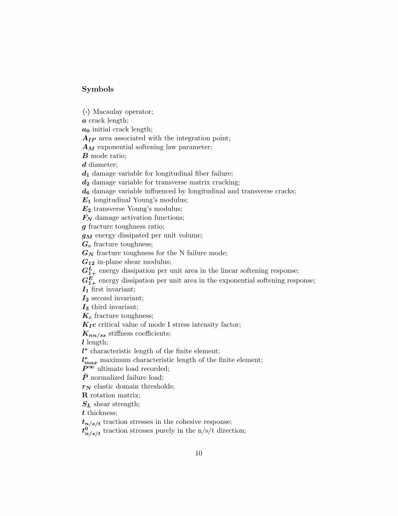
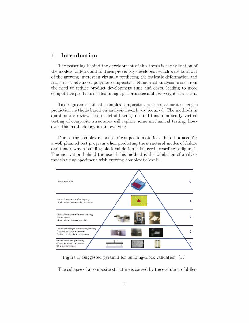
Due to the complex response of composite materials, there is a need fora well-planned test program when predicting the structural modes of failureand that is why a building block validation is followed according to figure 1.The motivation behind the use of this method is the validation of analysismodels using specimens with growing complexity levels.
Figure 1: Suggested pyramid for building-block validation. [15]
The collapse of a composite structure is caused by the evolution of differ-
14
ent damage mechanisms, namely matrix transverse cracking, fibre fractureand delamination. The exact sequence of failure mechanisms depends onthe loading, geometry, lay-up and stacking sequence.
The models proposed to predict the onset and propagation of the differ-ent damage mechanisms are implemented using Abaqus UEL (user subrou-tines) and VUMAT subroutines and the reasoning behind the developmentof the mesh and the limit element size is presented.
The thesis is organized in five different chapters: chapter 2 describesthe literature review performed on the Continuum Damage Model and theSmeared Crack Model; chapter 3 describes the experimental tests previouslyperformed to measure the material properties needed for the routines; chap-ter 4 shows the numerical results and how they compare to the experimentaldata for IM7/8552 under tensile and compressive loading; the last chapterpresents the main conclusions and suggestions for future work.
15
2 Literature Review
This chapter is mainly divided in two parts, the first part reviewing thetwo-dimensional models and the second part reviewing the three-dimensionalmodels, which would both be later on implemented in the user routines forthe numerical simulations.
2.1 2D Continuum Damage Model
Micro-mechanical models are ideal to design the material; they are not,however, suitable for structural analysis. In order to accomplish a modelthat gathers the advantages of both methods, arises the need to create amodel that links the micro and macro-mechanical scale.
2.1.1 Constitutive Model
When working with materials that accumulate damage before collapse,which is the case of advanced composites, fracture mechanics is not a suf-ficient enough method to predict ultimate failure; especially when it comesto multi-directional laminates, since they are able to sustain a significantamount of damage before collapse. Therefore, alternative solutions must beexplored [30].
Simplified models may be implemented, however, they do not have a sat-isfactory response when it comes to analysing materials with quasi-brittlefailure behaviour under general loading scenarios.
As an alternative, non-linear constitutive models may be implemented.This type of Continuum Damage Models allows the analysis of damage fromits onset to the final collapse, considering every ply as a homogenized ma-terial.
The model under review in this subsection has the advantage of work-ing with very simple parameters which can be obtained from standard testmethods. Another complementary advantage is related to the fact that theseparameters are ply-based characteristics, which means that they do not de-mand alterations every time the lay-up of the composite is redefined.
Another feature inherent to the model that is important to highlight isthat it accounts for crack closure effects under load reversal and therefore, al-
16
lows the study of non-loading where this phenomenon has an important role.
One of the main advantages of the developed model is that it guaranteescomputational efficiency due to the fact that it can be integrated explicitly,which allows its use for large scale computations. However, the model underconsideration does not allow the prediction of delamination, it focuses onlyon intralaminar failure such as matrix cracking and fibre fracture.
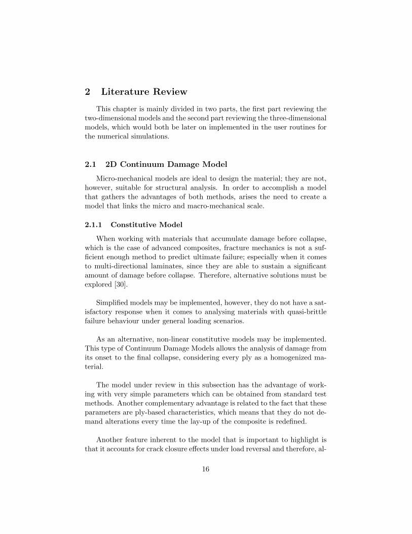
This method focuses on four different types of failure: transverse andlongitudinal, tension and compression.
Figure 2: Different types of fracture considered in the model. [30]
Analysing in detail the structure of the model, one needs to acknowledgedifferent parts: the constitutive law, the damage activation, the damage evo-lution and finally the softening constitutive law.
In order to define the constitutive law, it needs to be ensured that theirreversibility of the damage process is respected. With this in mind, a scalarfunction (complementary free energy density - G) is defined, insuring thatit is positive definite and that it is zero at the origin when it comes to thestresses:
G =σ2
11
2(1− d1)E1+
σ222
2(1− d2)E2−ν12
E1σ11σ22 +
σ212
2(1− d6)G12
+(α11σ11 + α22σ22)∆T + (β11σ11 + β22σ22)∆M
Like it was previously mentioned, the properties utilized here are at thelevel of each unidirectional lamina; E1, E2, ν12, G12, the in-plane elasticorthotropic properties; β11/22 are coefficients of hygroscopic expansion and,
17
also involved in the definition of the constitutive law, are α11/22, coeffi-cients of thermal expansion. The variables ∆M and ∆T are the differencesin temperature and moisture, respectively, compared to reference values.The representative volume to which the constitutive equations are appliedmust be larger than the diameter of the fibre.
Regarding the three scalar variables d1, d2 and d6, they correspond todifferent damage variables which represent different types of damage in ac-tion: longitudinal fiber failure (d1), transverse matrix cracking (d2) anddamage influenced by longitudinal and transverse cracks (d6). These vari-ables allow the definition of the domain of elastic response, essential for thedevelopment of the damage model.
In order to track whether the kind of damage mechanisms in action isdue to compression or tension, fiber failure or matrix cracking, the damagemodes are defined in the following way:
d1 = d1+〈σ11〉|σ11|
+ d1−〈−σ11〉|σ11|
d2 = d2+〈σ22〉|σ22|
+ d2−〈−σ22〉|σ22|
Knowing that 〈x〉 is the Macaulay operator, and so, 〈x〉 = (x+ |x|)/2.
2.1.1.1 Damage activation functions
To determine the type of damage initiated, four damage activation func-tions, F1+, F1−, F2+, F2−, are defined. These functions are based on theLaRC03 and LaRC04 criteria; the latter being used selectively, due to itsincreasing computational needs. These criteria do not require curve-fittingparameters and have no restrictions regarding loading combinations [11].
Graphically, the four damage activation variables represent different sur-faces that constrict the elastic domain, a space where the material is linearelastic and when one becomes positive, the material’s response is no longerelastic and there is damage evolution. The functions FN are defined accord-ing to the following expressions:
F1+ = φ1+ − r1+ 6 0
18
F1− = φ1− − r1− 6 0
F2+ = φ2+ − r2+ 6 0
F2− = φ2− − r2− 6 0
Where φN represents the loading function that depends on strain ten-sor and material constants and rN represent the elastic domain thresholdswhich are related to the damage variables (dN ) and take the value of 1 whenthe material is undamaged and increase with damage.
2.1.1.1.1 Damage activation functions in longitudinal fracture
For longitudinal tension, a non-interactive strain criterion based on theLaRC04 criterion is used to define the loading function as shown:
φ1+ =E1
XTε11
However, in longitudinal compression, since there is damage onset in thematrix, a loss of lateral support for the fibres leads to a formation of a kinkband. In these conditions, the loading function is established according tothe LaRC03 criterion and takes form as:
φ1− =〈|σm12|+ ηLσm22〉
SL
Where ηL represents the longitudinal friction coefficient as determinedin [24] and the σm represents the stress tensor in the coordinate system ofthe misaligned fiber plane. This criterion’s development asks for the inputof the misalignment angle of the fibres which is a function of the appliedstress. However, as a simplification, the model uses a constant angle thatcorresponds to the one in a pure longitudinal compression scenario.
2.1.1.1.2 Damage activation functions in transverse fracture
Depending on the type of loading that leads to transverse fracture, thematerial might crack perpendicularly to the mid-plane of the ply (α0 = 0◦)or with a crack plane angle of 53◦. The cases described correspond respec-tively to in-plane shear stresses combined with transverse tensile stresses
19
or to in-plane shear stresses combined with small transverse compressivestresses and high transverse stresses.
Using the LaRC04 criterion, both cases are analysed, leading to threedifferent expressions for the loading functions as presented:
φ2+ =
√(1− g)
σ22
YT+ g
(σ22
YT
)2
+
(σ12
SL
)2
if σ12 > 0
φ2+ =1
SL〈|σ12|+ ηLσ22〉 if σ12 < 0
For α0 = 0◦ and where g = GIcGIIc
, i.e. it represents the fracture tough-ness ratio.
φ2− =
√√√√( τTeffST
)2
+
(τLeff
SL
)2
if σ12 < 0
For α0 = 53◦ and where τT/Leff represents the effective stresses defined
in [33].
Under transverse fracture where compression is principal, the fractureangle is indeed approximately 53◦ in carbon-epoxy composites. However,with increasing in-plane shear, the angle diminishes, going through 40◦ andultimately reaching 0◦. With computational efficiency in mind, the modelallows only discrete values of 53◦ and 0◦,
2.1.1.2 Damage evolution
Damage evolution is defined by the Kuhn-Tucker conditions that can berepresented as:
rN > 0; FN 6 0; rNFN = 0
This means that while FN is negative, the material has an elastic be-haviour but when it reaches 0 and other conditions are met, there is damageevolution.
Even though during damage evolution there is an active elastic domainbeing analysed, the model still accompanies the evolution of the other elas-tic domains; always assuming that transverse and longitudinal domains are
20
never coupled.
2.1.1.3 Softening laws
In order to ensure a safe implementation of the softening constitutiveequations, the Bazants crack band model is implemented for each intralam-inar failure mode in question with the addition of a definition of the maxi-mum size of the finite elements.
This is implemented regularizing the computed dissipated energy withthe use of a characteristic dimension of the finite element and the fracturetoughness [28], which leads to:
gM =GM
l∗,M = 1±, 2±, 6
Where GM is the fracture toughness, gM is the energy dissipated per unitvolume, and l∗ is the characteristic length of the finite element. For squareelements, the characteristic element length can be approximated by the fol-lowing expression:
l∗ =
√AIP
cos(γ)
Where |γ| ≤ 45◦ is the angle of the mesh lines with the crack direction andAIP is the area associated with each integration point.
The crack band model uses an approximation to represent the failureprocess zone by a damaged finite element zone with the width of one ele-ment as to achieve an appropriate response to complex mechanisms in largestructures.
As soon as one of the FN is activated, the damage evolution laws aretriggered in order to represent the cohesive response which is linear untilthe stress reaches the pull-out stress, XPO, and the corresponding energydissipation per unit area is GL1+. As the strains continue to increase, thesoftening response follows an exponential law and the energy dissipated perunit area is GE1+ [31] as can be seen in figure 3.
21
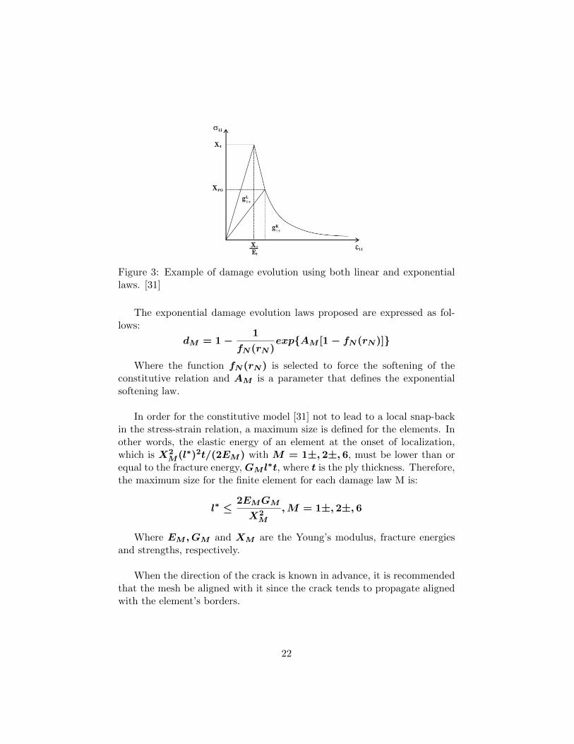
Figure 3: Example of damage evolution using both linear and exponentiallaws. [31]
The exponential damage evolution laws proposed are expressed as fol-lows:
dM = 1−1
fN(rN)exp{AM [1− fN(rN)]}
Where the function fN(rN) is selected to force the softening of theconstitutive relation and AM is a parameter that defines the exponentialsoftening law.
In order for the constitutive model [31] not to lead to a local snap-backin the stress-strain relation, a maximum size is defined for the elements. Inother words, the elastic energy of an element at the onset of localization,which is X2
M(l∗)2t/(2EM) with M = 1±, 2±, 6, must be lower than orequal to the fracture energy, GM l
∗t, where t is the ply thickness. Therefore,the maximum size for the finite element for each damage law M is:
l∗ ≤2EMGM
X2M
,M = 1±, 2±, 6
Where EM , GM and XM are the Young’s modulus, fracture energiesand strengths, respectively.
When the direction of the crack is known in advance, it is recommendedthat the mesh be aligned with it since the crack tends to propagate alignedwith the element’s borders.
22
With the evolution law defined, the integration of the rate at which theenergy is dissipated associated with the definition of characteristic lengthleads to proof of the independence from mesh size.
In addition, it is important to refer that only half of the specimen ismodelled in order to reduce computation efforts. Also, since a maximumelement size is defined but not always possible to enforce, a strategy is de-fined as to automatically lower the strength of the bigger elements, keepingthe fracture toughness constant.
2.2 3D Constitutive Models
The model under review in this section uses a three-dimensional SmearedCrack Model to predict the onset and propagation of failure in transversecracking and a modification of the previously described 2D model ([30] and[31]) to represent the longitudinal failure. The main concern here is to anal-yse more complicated stress states and to account for the plastic deformationof the polymer resin that precedes the cracking of the plies [15].
The validation process is also more complete, applying a building-blockvalidation model of five levels of growing complexity. This approach guar-antees that costs are minimized while performance objectives are met, sincesmaller and cheaper specimens are tested first, and only when technologyrisks are assessed, does the level of complexity of the tests increase.
In order to predict compressive and tensile transverse matrix cracking,the model proposes a 3D invariant-based criterion that is formulated di-rectly from the yield function presented in [40]. This formulation defines a,the preferred direction in transversely isotropic materials, around which thematerial’s response is invariant with respect to arbitrary rotations.
There is also the need to specify a structural tensor of transverse isotropy,A, representing the material’s intrinsic characteristic direction [14]. Havingdefined all the elements, the failure indexes φ2± can now be reached accord-ing to the expressions presented in [14] that lead to:
φ2± = α1I1 + α2I2 + α3I3 + α32I23 ≤ 1
With: α3 = αt3, α32 = αt32 if I3 > 0 and α3 = αc3, α32 = αc32 if I3 ≤ 0.
23
The proposed failure criteria allows for the study of failure under biaxialstress states to be made and the six failure parameters (α1, α2, α
t3, α
c3, α
t32
and αc32) are functions of the transverse and in-plane shear strengths, thetransverse tensile and compressive strengths, and the biaxial transverse ten-sile and compressive strengths [14].
The criterion defined provides feasible predictions for the different loadcases analysed.
Once defined the onset of transverse failure, it is now necessary to sim-ulate the cracks under general loading. Since the orientation of the crackplane depends on the stress state, it is not possible to use cohesive zonemodels and so a Smeared Crack Model based on the work presented in [28]is used.
2.2.1 Damage Model for transverse fracture - SCM
A Smeared Crack Model is a constitutive model specifically developedfor quasibrittle materials in which the total strain is considered a summationof two parts: the strain correspondent to the deformation of the uncrackedmaterial and the additional deformation due to the opening of cracks.
ε = εe + εc = εe + R · εcrc ·RT
Where εcrc is the cracking strain projected in the coordinate system of thecrack and R is the rotation matrix, whose components are defined by thefailure criteria [15].
As mentioned before, the transverse fracture under compressive load-ing leads to a fracture angle that, in the case of a simple stress state incarbon-epoxy composites, is 53◦. However, in this case, a more complexstress states is being analysed and thus the use of a rotation matrix thatcalculates the angle of fracture at the onset of the crack. Further along inthe model, that angle is considered a constant, i.e., a rotating crack is notanalysed.
At this point, a projection of the tractions acting on the fracture planeonto the crack frame is made and now the displacement jumps must berelated to the tractions. This correlation is done using a cohesive law basedon that developed by Turon [39] but bearing in mind that the linear softening
24
cohesive law must be adapted to the Smeared Crack Model. This said, thetractions acting on the fracture plane are defined as:
tcri =
(1− dd
)ωcriωmi
tcri −δi2〈−ωcr2 〉|ωcr2 |
[(1− dd
)ωcriωmf
tcri − E2(εcr22 − εcrc22)
]
Knowing that:δij : Kroenecker delta;ωmf : equivalent displacement jump at failure under mixed-mode loadingconditions;ωcri : scalar components of the displacement vector;εcr22 and εcrc22: scalar components of strain and cracking strain tensors, re-spectively;〈·〉: Macaulay operator defined before.
The damage variable (d) is obtained using a loading function defined as
L (ωcr) = min{λωmf, 1}
where λ is the equivalent displacement jump.
To predict the mixed-mode interlaminar fracture toughness of compositelaminates, the B-K criterion [13], a criterion based on energy release rate,is used. Both the linear criterion and the B-K criterion would be applicablehere, however, the latter provides additional flexibility since it has an addi-tional material parameter (η) [15]. The development of this criterion occursas such:
Gc = Gic +ABη
With the mode ratio beingB = tcrs ββ(tcrs −tcr2 )+tcr2
, the mixed-mode fracture
toughness being Gc = 2(Gic+ABη)
tcrand A = GIIc −GIc.
2.2.2 Damage Model for longitudinal fracture - CDM
Since the SCM does not permit the representation of some mechanismsof longitudinal failure - non matrix dominated ones - the same failure crite-rion as in the 2D model [30] must be implemented in this field with somemodifications.
The function that predicts longitudinal tensile fracture is the maximumstrain criterion:
φ1− =ε11
εT1
25
When compressive loading is longitudinally applied, the effects of fiberkinking are relevant and must be predicted. In order to do so, the hypothesisput forward by Argon in [9] is used to develop the model. The hypothesisassumes that kink bands are triggered by localized matrix failure in thevicinity of misaligned fibres [9].
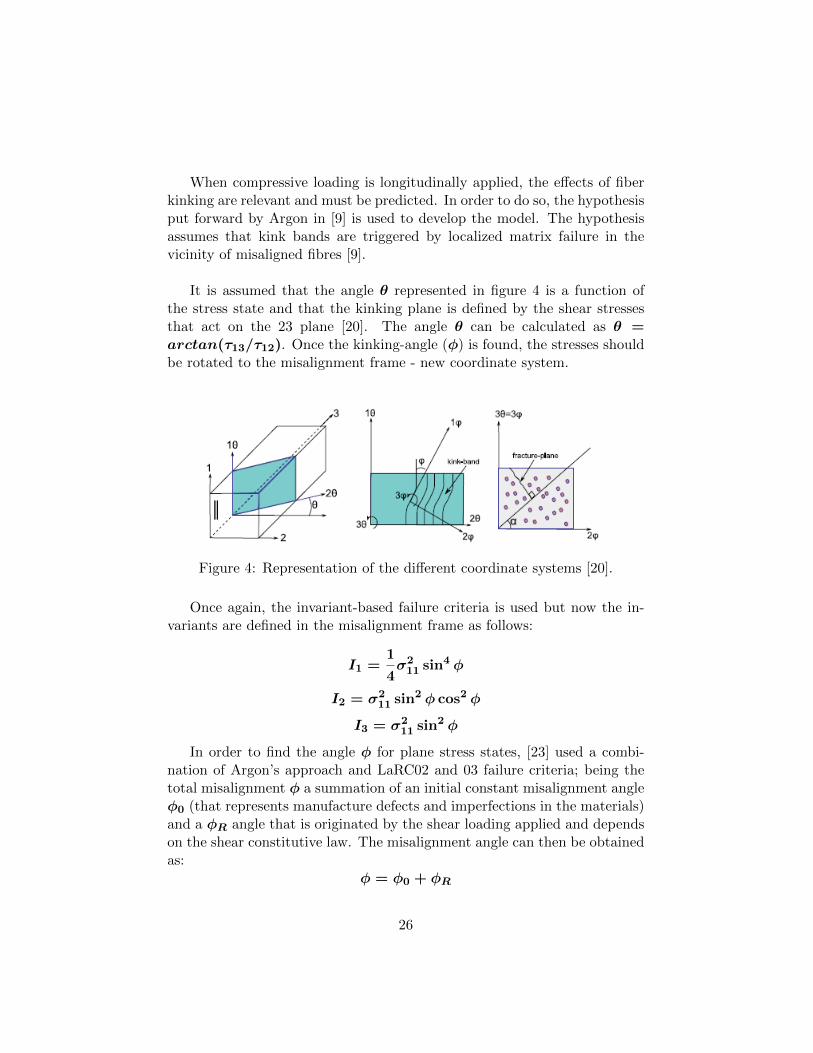
It is assumed that the angle θ represented in figure 4 is a function ofthe stress state and that the kinking plane is defined by the shear stressesthat act on the 23 plane [20]. The angle θ can be calculated as θ =arctan(τ13/τ12). Once the kinking-angle (φ) is found, the stresses shouldbe rotated to the misalignment frame - new coordinate system.
Figure 4: Representation of the different coordinate systems [20].
Once again, the invariant-based failure criteria is used but now the in-variants are defined in the misalignment frame as follows:
I1 =1
4σ2
11 sin4 φ
I2 = σ211 sin2 φ cos2 φ
I3 = σ211 sin2 φ
In order to find the angle φ for plane stress states, [23] used a combi-nation of Argon’s approach and LaRC02 and 03 failure criteria; being thetotal misalignment φ a summation of an initial constant misalignment angleφ0 (that represents manufacture defects and imperfections in the materials)and a φR angle that is originated by the shear loading applied and dependson the shear constitutive law. The misalignment angle can then be obtainedas:
φ = φ0 + φR
26
When it comes to damage evolution, just as in the 2D model analysedin another section, a bi-linear softening law is required, so as not to overpredict the peak load in fiber dominated failure.
Once again, the characteristic length (l∗) is used in this model as to en-sure the independence from the element size. The same l∗ will be consideredin both transverse and longitudinal modes.
A consequence of the increasing complexity of the validation models isthat, with different specimens, different specifications arise. For example,in the case of specimens with geometrical discontinuities, the stress ten-sor has non-zero out-of-plane components which may lead to delaminationand therefore, the use of cohesive finite elements or surfaces must be imple-mented in-between the plies.
27
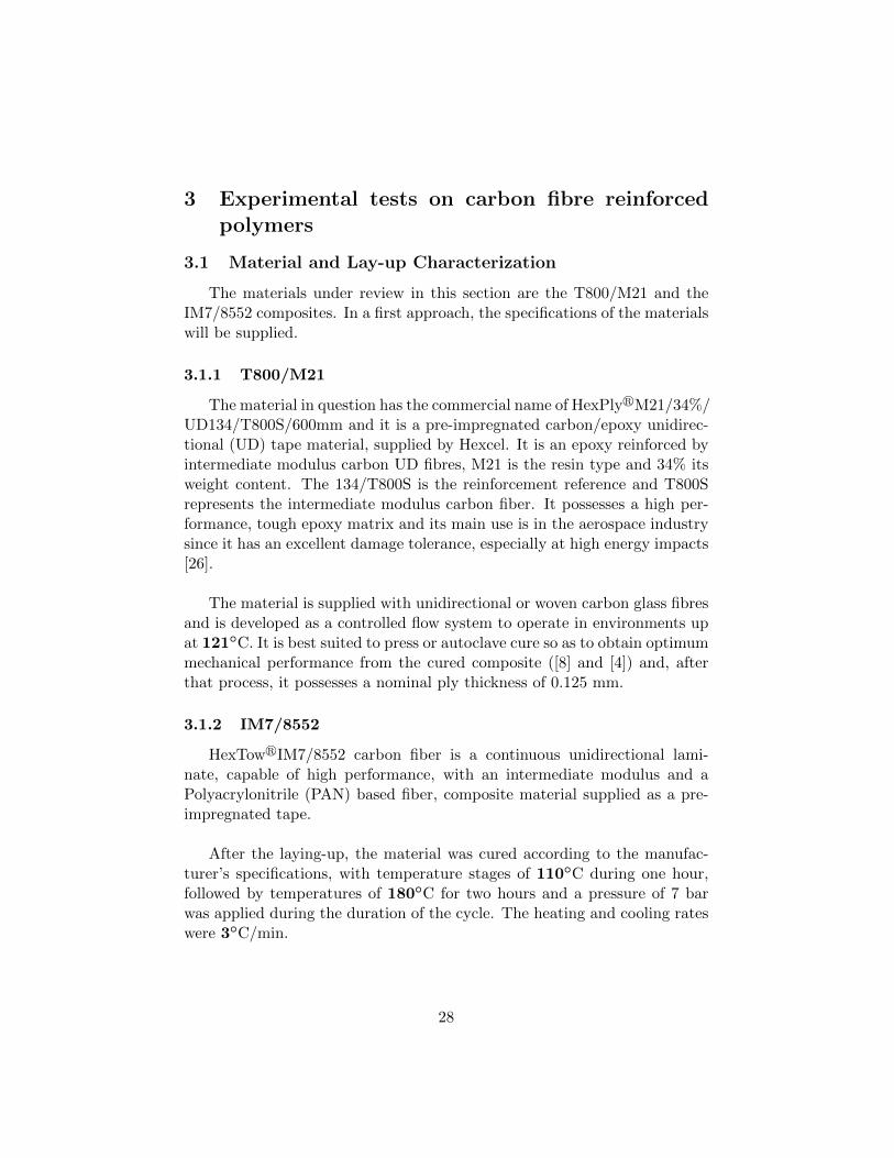
3 Experimental tests on carbon fibre reinforcedpolymers
3.1 Material and Lay-up Characterization
The materials under review in this section are the T800/M21 and theIM7/8552 composites. In a first approach, the specifications of the materialswill be supplied.
3.1.1 T800/M21
The material in question has the commercial name of HexPlyrM21/34%/UD134/T800S/600mm and it is a pre-impregnated carbon/epoxy unidirec-tional (UD) tape material, supplied by Hexcel. It is an epoxy reinforced byintermediate modulus carbon UD fibres, M21 is the resin type and 34% itsweight content. The 134/T800S is the reinforcement reference and T800Srepresents the intermediate modulus carbon fiber. It possesses a high per-formance, tough epoxy matrix and its main use is in the aerospace industrysince it has an excellent damage tolerance, especially at high energy impacts[26].
The material is supplied with unidirectional or woven carbon glass fibresand is developed as a controlled flow system to operate in environments upat 121◦C. It is best suited to press or autoclave cure so as to obtain optimummechanical performance from the cured composite ([8] and [4]) and, afterthat process, it possesses a nominal ply thickness of 0.125 mm.
3.1.2 IM7/8552
HexTowrIM7/8552 carbon fiber is a continuous unidirectional lami-nate, capable of high performance, with an intermediate modulus and aPolyacrylonitrile (PAN) based fiber, composite material supplied as a pre-impregnated tape.
After the laying-up, the material was cured according to the manufac-turer’s specifications, with temperature stages of 110◦C during one hour,followed by temperatures of 180◦C for two hours and a pressure of 7 barwas applied during the duration of the cycle. The heating and cooling rateswere 3◦C/min.
28
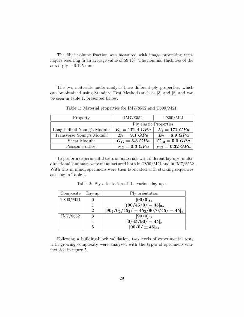
The fiber volume fraction was measured with image processing tech-niques resulting in an average value of 59.1%. The nominal thickness of thecured ply is 0.125 mm.
The two materials under analysis have different ply properties, whichcan be obtained using Standard Test Methods such as [3] and [8] and canbe seen in table 1, presented below.
Table 1: Material properties for IM7/8552 and T800/M21.
Property IM7/8552 T800/M21
Ply elastic Properties
Longitudinal Young’s Moduli: E1 = 171.4 GPa E1 = 172 GPa
Transverse Young’s Moduli: E2 = 9.1 GPa E2 = 8.9 GPa
Shear Moduli: G12 = 5.3 GPa G12 = 5.0 GPa
Poisson’s ratios: ν12 = 0.3 GPa ν12 = 0.32 GPa
To perform experimental tests on materials with different lay-ups, multi-directional laminates were manufactured both in T800/M21 and in IM7/8552.With this in mind, specimens were then fabricated with stacking sequencesas show in Table 2.
Table 2: Ply orientation of the various lay-ups.
Composite Lay-up Ply orientation
T800/M21 0 [90/0]8s1 [(90/45/0/− 45]3s2 [902/02/452/− 452/90/0/45/− 45]s
IM7/8552 3 [90/0]8s4 [0/45/90/− 45]s5 [90/0/± 45]3s
Following a building-block validation, two levels of experimental testswith growing complexity were analysed with the types of specimens enu-merated in figure 5.
29
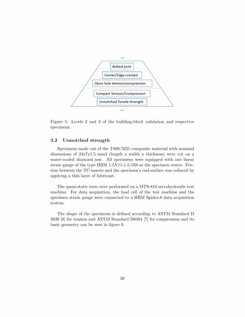
Figure 5: Levels 2 and 3 of the building-block validation and respectivespecimens.
3.2 Unnotched strength
Specimens made out of the T800/M21 composite material with nominaldimensions of 23x7x1.5 mm3 (length x width x thickness) were cut on awater-cooled diamond saw. All specimens were equipped with one linearstrain gauge of the type HBM 1-LY11-1.5/350 at the specimen centre. Fric-tion between the TC-inserts and the specimen’s end-surface was reduced byapplying a thin layer of lubricant.
The quasi-static tests were performed on a MTS-810 servohydraulic testmachine. For data acquisition, the load cell of the test machine and thespecimen strain gauge were connected to a HBM Spider-8 data acquisitionsystem.
The shape of the specimens is defined according to ASTM Standard D3039 [8] for tension and ASTM Standard D6484 [7] for compression and itsbasic geometry can be seen in figure 6.
30
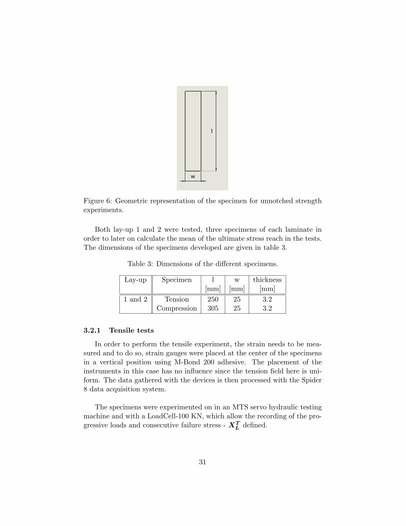
Figure 6: Geometric representation of the specimen for unnotched strengthexperiments.
Both lay-up 1 and 2 were tested, three specimens of each laminate inorder to later on calculate the mean of the ultimate stress reach in the tests.The dimensions of the specimens developed are given in table 3.
Table 3: Dimensions of the different specimens.
Lay-up Specimen l w thickness[mm] [mm] [mm]
1 and 2 Tension 250 25 3.2Compression 305 25 3.2
3.2.1 Tensile tests
In order to perform the tensile experiment, the strain needs to be mea-sured and to do so, strain gauges were placed at the center of the specimensin a vertical position using M-Bond 200 adhesive. The placement of theinstruments in this case has no influence since the tension field here is uni-form. The data gathered with the devices is then processed with the Spider8 data acquisition system.
The specimens were experimented on in an MTS servo hydraulic testingmachine and with a LoadCell-100 KN, which allow the recording of the pro-gressive loads and consecutive failure stress - XT
L defined.
31
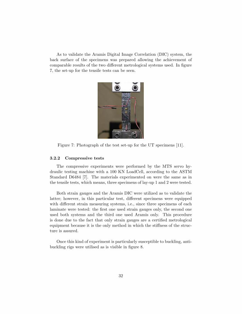
As to validate the Aramis Digital Image Correlation (DIC) system, theback surface of the specimens was prepared allowing the achievement ofcomparable results of the two different metrological systems used. In figure7, the set-up for the tensile tests can be seen.
Figure 7: Photograph of the test set-up for the UT specimens [11].
3.2.2 Compressive tests
The compressive experiments were performed by the MTS servo hy-draulic testing machine with a 100 KN LoadCell, according to the ASTMStandard D6484 [7]. The materials experimented on were the same as inthe tensile tests, which means, three specimens of lay-up 1 and 2 were tested.
Both strain gauges and the Aramis DIC were utilized as to validate thelatter; however, in this particular test, different specimens were equippedwith different strain measuring systems, i.e., since three specimens of eachlaminate were tested: the first one used strain gauges only, the second oneused both systems and the third one used Aramis only. This procedureis done due to the fact that only strain gauges are a certified metrologicalequipment because it is the only method in which the stiffness of the struc-ture is assured.
Once this kind of experiment is particularly susceptible to buckling, anti-buckling rigs were utilised as is visible in figure 8.
32
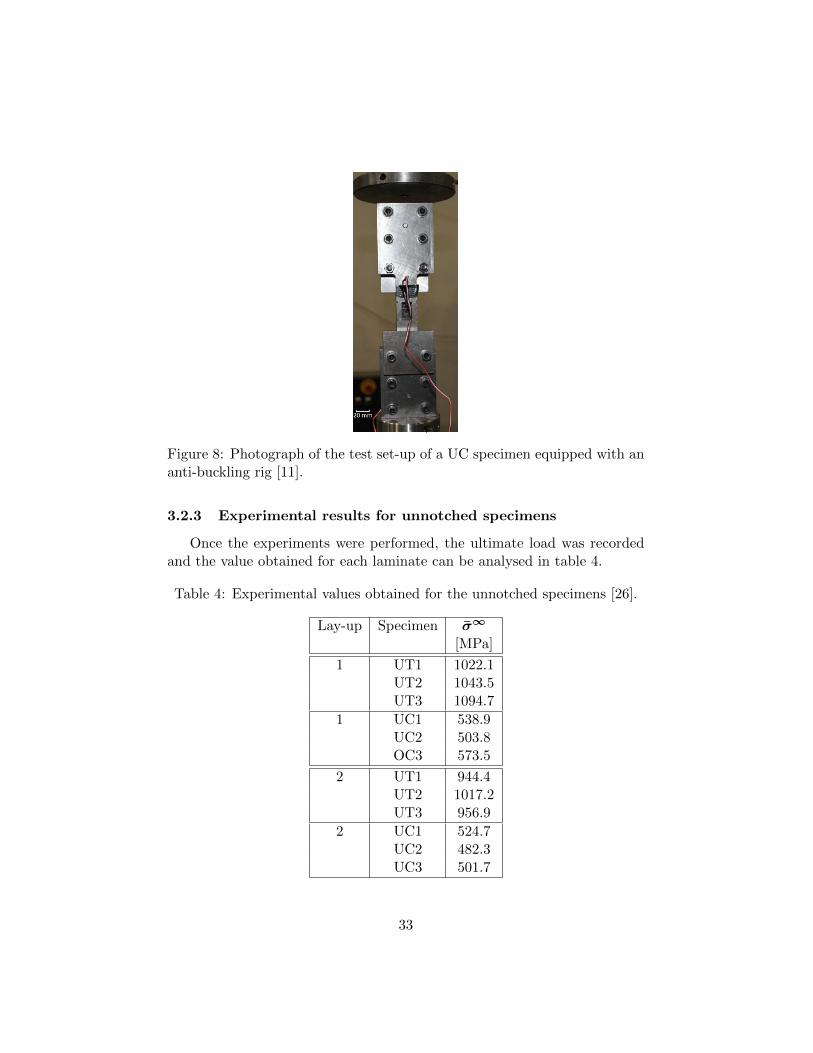
Figure 8: Photograph of the test set-up of a UC specimen equipped with ananti-buckling rig [11].
3.2.3 Experimental results for unnotched specimens
Once the experiments were performed, the ultimate load was recordedand the value obtained for each laminate can be analysed in table 4.
Table 4: Experimental values obtained for the unnotched specimens [26].
Lay-up Specimen σ∞
[MPa]
1 UT1 1022.1UT2 1043.5UT3 1094.7
1 UC1 538.9UC2 503.8OC3 573.5
2 UT1 944.4UT2 1017.2UT3 956.9
2 UC1 524.7UC2 482.3UC3 501.7
33
The mean of the values presented in the table above leads to the lami-nates’ unnotched compressive and tensile strengths which are presented inthe following table.
Table 5: Mean of the experimental values obtained for the unnotched spec-imens [26].
Lay-up XTL XC
L
[MPa] [MPa]
1 1053.5 538.72 972.8 502.9
3.3 Compact Tension and Compression
Compact Tension and Compression tests were performed so that thefracture toughness associated with longitudinal failure would be obtainedfor the T800/M21 composite, for lay-up 0.
The tests were not performed according to any standard because onedoes not yet exist. However, a procedure has been developed ([10],[27], [34],[29], [16], [21]) and a simple explanation of it will be presented in this chap-ter.
The material was loaded using the MTS-LoadCell-100 KN testing ma-chine at a constant velocity of 2 mm/min in the direction of the 0◦ lami-nates. The elastic properties of the laminate were then calculated by usingESAComp 3.5 [1].
In order to obtain strain values, the surface of the material was paintedwhite with black dots as speckle pattern, which allows the use of AramisDIC.
In this test, it is important to focus on the likelihood of buckling occur-rence due to the high loads required to propagate the crack. In order tominimize its existence, steel anti-buckling rigs were introduced to the exper-iment [26].
34
3.3.1 Tension
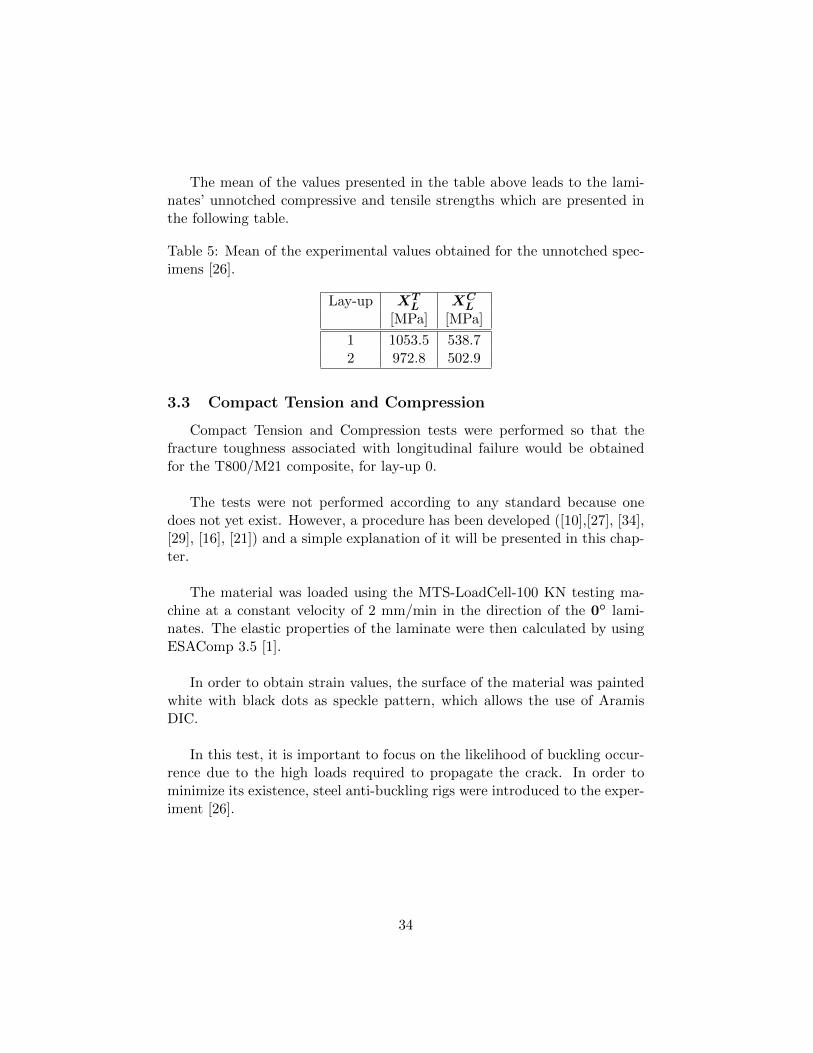
The specimens used to perform the compact tension experiment can beseen in a simplified representation in figure 9, below, and their dimensionsin table 6.
Figure 9: Geometric representation of the specimen for Compact Tensionexperiments.
Table 6: Dimensions of the Compact Tension specimens.
l w c d s e R t
67 mm 67 mm 32 mm 10 mm 4 mm 30 mm 6.5 mm 4 mm
In these tests, an attainment of a smooth speckle pattern in the surfaceof the T800/M21 composite was difficult and so, the Aramis measurementswere deemed invalid.
As an alternative, a ruler with real mm scale was attached to the surfaceof the specimen near the notch’s edge where the opening of the crack occurs -see figure 10. Then, with the help of photographic evidence, the propagationof the crack is analysed.
35
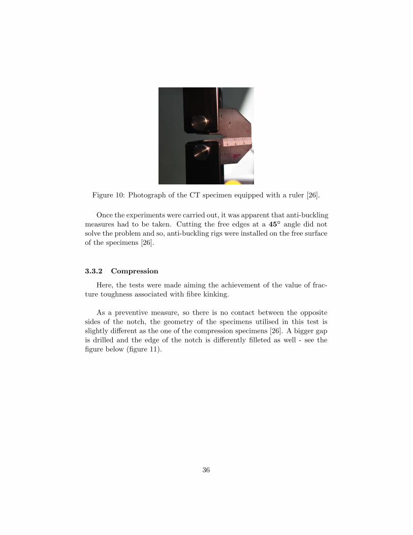
Figure 10: Photograph of the CT specimen equipped with a ruler [26].
Once the experiments were carried out, it was apparent that anti-bucklingmeasures had to be taken. Cutting the free edges at a 45◦ angle did notsolve the problem and so, anti-buckling rigs were installed on the free surfaceof the specimens [26].
3.3.2 Compression
Here, the tests were made aiming the achievement of the value of frac-ture toughness associated with fibre kinking.
As a preventive measure, so there is no contact between the oppositesides of the notch, the geometry of the specimens utilised in this test isslightly different as the one of the compression specimens [26]. A bigger gapis drilled and the edge of the notch is differently filleted as well - see thefigure below (figure 11).
36
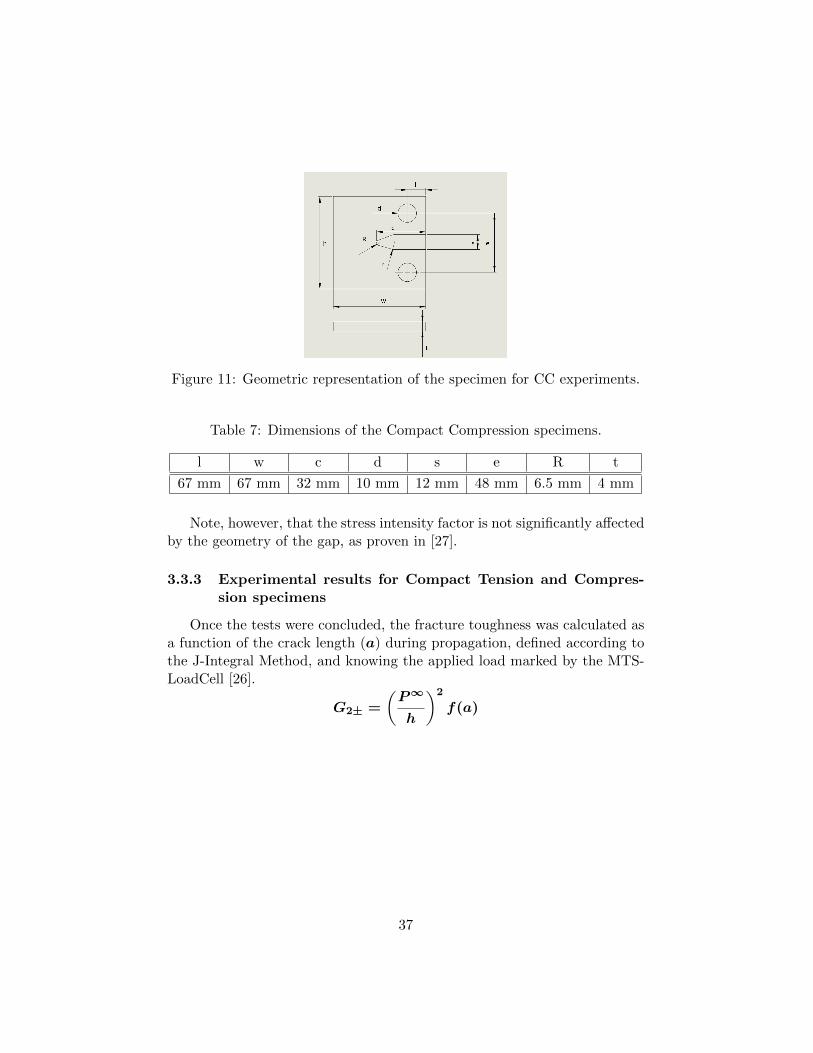
Figure 11: Geometric representation of the specimen for CC experiments.
Table 7: Dimensions of the Compact Compression specimens.
l w c d s e R t
67 mm 67 mm 32 mm 10 mm 12 mm 48 mm 6.5 mm 4 mm
Note, however, that the stress intensity factor is not significantly affectedby the geometry of the gap, as proven in [27].
3.3.3 Experimental results for Compact Tension and Compres-sion specimens
Once the tests were concluded, the fracture toughness was calculated asa function of the crack length (a) during propagation, defined according tothe J-Integral Method, and knowing the applied load marked by the MTS-LoadCell [26].
G2± =
(P∞
h
)2
f(a)
37
Table 8: Experimental values obtained for the Compact Tension and Com-pression specimens [26].
Lay-up Specimen P∞ G2+ G2−[N] [J/mm2] [J/mm2]
0 CT1 6890.6 100.5CT2 - -CT3 - -CT4 6076.6 84.5
0 CC1 -4743.5 89.5CC2 -4721.4 88.6CC3 -4383.4 76.4CC4 -4652.4 86.1
From the table above, one may reach the conclusion that the longi-tudinal compressive fracture toughness, G2− for the [90/0]8s laminate is85.1J/mm2. The longitudinal tensile fracture toughness, G2+, on theother hand, may only be estimated as 92.5J/mm2 since two of the tensionspecimens buckled and just the initiation values of the laminate fracturetoughness were used [26].
3.4 Center-Cracked
The experiment under review in this chapter has the purpose of mea-suring the fracture toughness of specimens with different notch dimensions.However, the basic geometry of the specimens is the same for all experimentsand can be seen in figure 12.
38
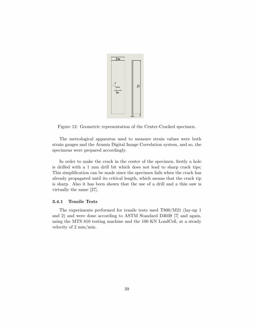
Figure 12: Geometric representation of the Center-Cracked specimen.
The metrological apparatus used to measure strain values were bothstrain gauges and the Aramis Digital Image Correlation system, and so, thespecimens were prepared accordingly.
In order to make the crack in the center of the specimen, firstly a holeis drilled with a 1 mm drill bit which does not lead to sharp crack tips;This simplification can be made since the specimen fails when the crack hasalready propagated until its critical length, which means that the crack tipis sharp. Also it has been shown that the use of a drill and a thin saw isvirtually the same [27].
3.4.1 Tensile Tests
The experiments performed for tensile tests used T800/M21 (lay-up 1and 2) and were done according to ASTM Standard D3039 [7] and again,using the MTS 810 testing machine and the 100 KN LoadCell, at a steadyvelocity of 2 mm/min.
39
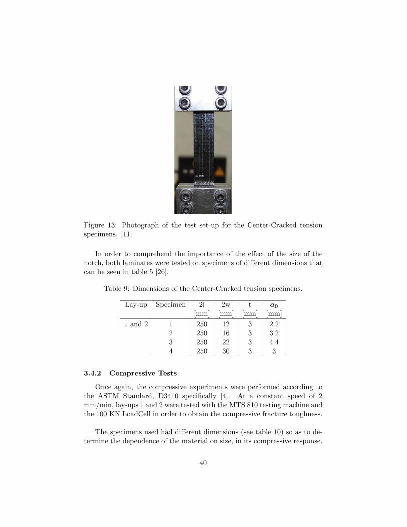
Figure 13: Photograph of the test set-up for the Center-Cracked tensionspecimens. [11]
In order to comprehend the importance of the effect of the size of thenotch, both laminates were tested on specimens of different dimensions thatcan be seen in table 5 [26].
Table 9: Dimensions of the Center-Cracked tension specimens.
Lay-up Specimen 2l 2w t a0
[mm] [mm] [mm] [mm]
1 and 2 1 250 12 3 2.22 250 16 3 3.23 250 22 3 4.44 250 30 3 3
3.4.2 Compressive Tests
Once again, the compressive experiments were performed according tothe ASTM Standard, D3410 specifically [4]. At a constant speed of 2mm/min, lay-ups 1 and 2 were tested with the MTS 810 testing machine andthe 100 KN LoadCell in order to obtain the compressive fracture toughness.
The specimens used had different dimensions (see table 10) so as to de-termine the dependence of the material on size, in its compressive response.
40
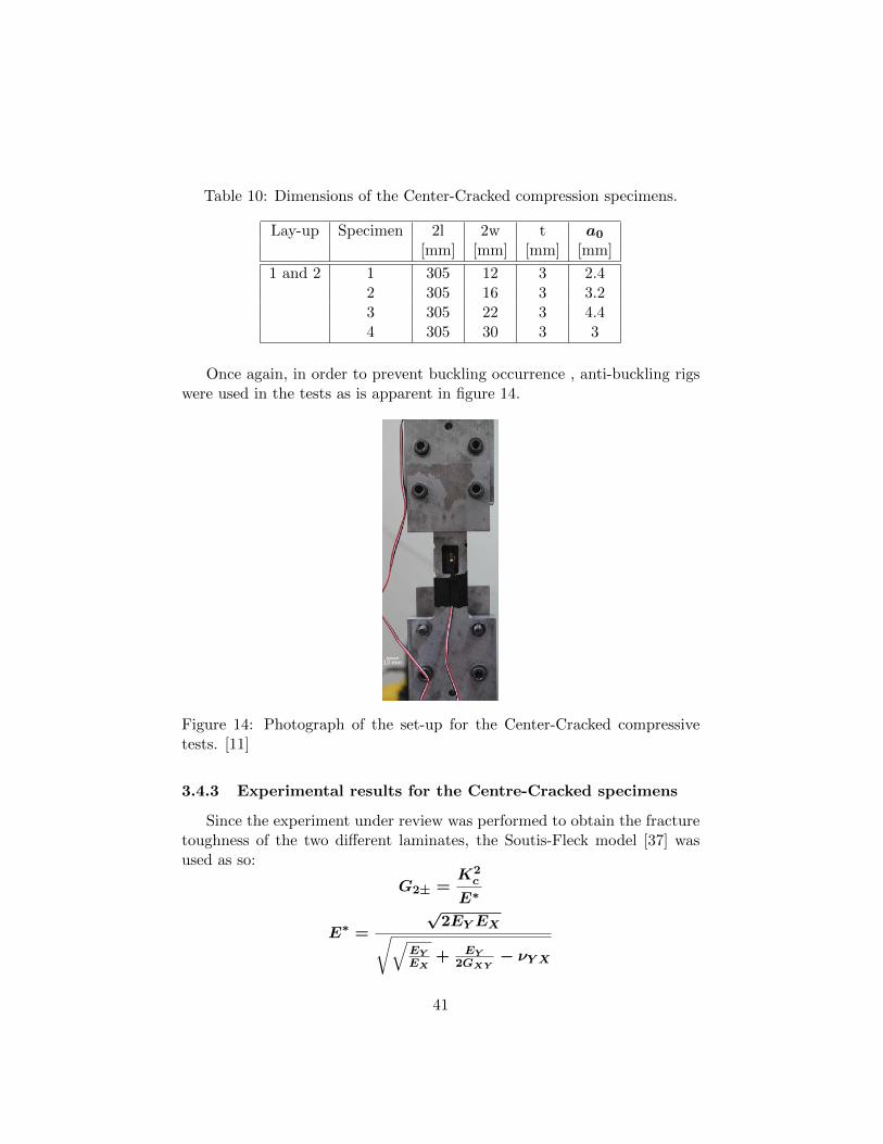
Table 10: Dimensions of the Center-Cracked compression specimens.
Lay-up Specimen 2l 2w t a0
[mm] [mm] [mm] [mm]
1 and 2 1 305 12 3 2.42 305 16 3 3.23 305 22 3 4.44 305 30 3 3
Once again, in order to prevent buckling occurrence , anti-buckling rigswere used in the tests as is apparent in figure 14.
Figure 14: Photograph of the set-up for the Center-Cracked compressivetests. [11]
3.4.3 Experimental results for the Centre-Cracked specimens
Since the experiment under review was performed to obtain the fracturetoughness of the two different laminates, the Soutis-Fleck model [37] wasused as so:
G2± =K2c
E∗
E∗ =
√2EY EX√√
EYEX
+ EY2GXY
− νY X
41
Kc = Y σ∞√πa
Where σ∞ is the remote stress at failure measured in the tests, Y is thefinite width correction factor, function of the w and a0 present in figure 12.The elastic properties enunciated were calculated using lamination theorywith the axis x aligned with the loading direction [26].
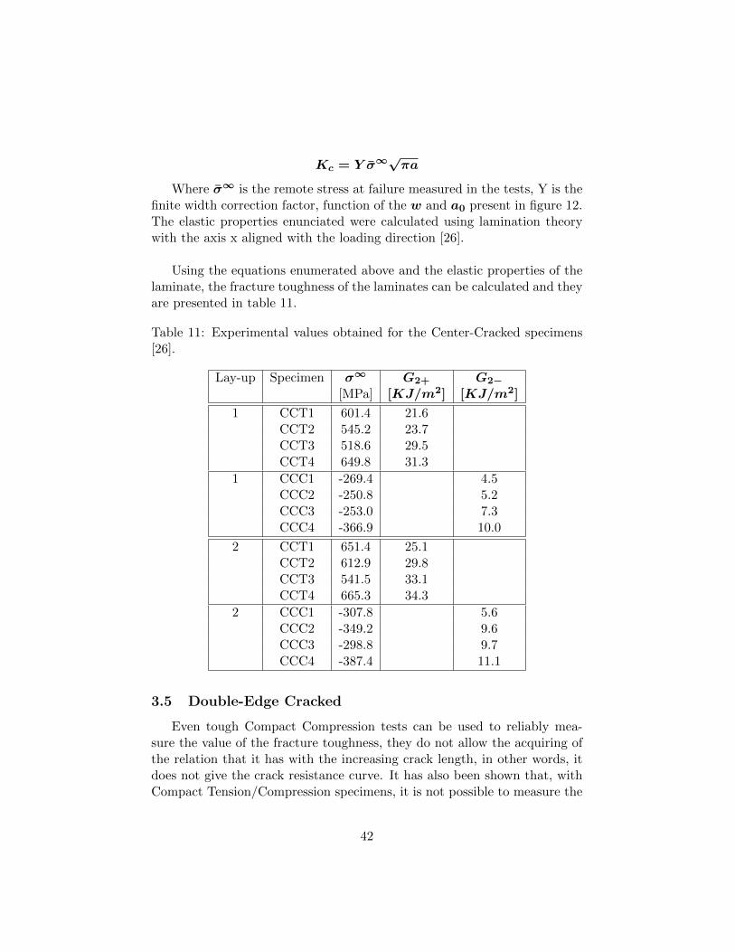
Using the equations enumerated above and the elastic properties of thelaminate, the fracture toughness of the laminates can be calculated and theyare presented in table 11.
Table 11: Experimental values obtained for the Center-Cracked specimens[26].
Lay-up Specimen σ∞ G2+ G2−[MPa] [KJ/m2] [KJ/m2]
1 CCT1 601.4 21.6CCT2 545.2 23.7CCT3 518.6 29.5CCT4 649.8 31.3
1 CCC1 -269.4 4.5CCC2 -250.8 5.2CCC3 -253.0 7.3CCC4 -366.9 10.0
2 CCT1 651.4 25.1CCT2 612.9 29.8CCT3 541.5 33.1CCT4 665.3 34.3
2 CCC1 -307.8 5.6CCC2 -349.2 9.6CCC3 -298.8 9.7CCC4 -387.4 11.1
3.5 Double-Edge Cracked
Even tough Compact Compression tests can be used to reliably mea-sure the value of the fracture toughness, they do not allow the acquiring ofthe relation that it has with the increasing crack length, in other words, itdoes not give the crack resistance curve. It has also been shown that, withCompact Tension/Compression specimens, it is not possible to measure the
42
fracture toughness of modern resin systems which lead to higher values offracture toughness [26]. With this in mind, Double-Edge Cracked specimenswere used to perform tensile and compressive experiments. Both T800/M21and IM7/8552 were utilised in this experiment with the lay-ups 0 and 3.
So as to follow the propagation of the crack, all the specimens werepainted white with a speckle, permitting the use of the Digital Image Cor-relation (DIC) system.
3.5.1 Tensile Tests
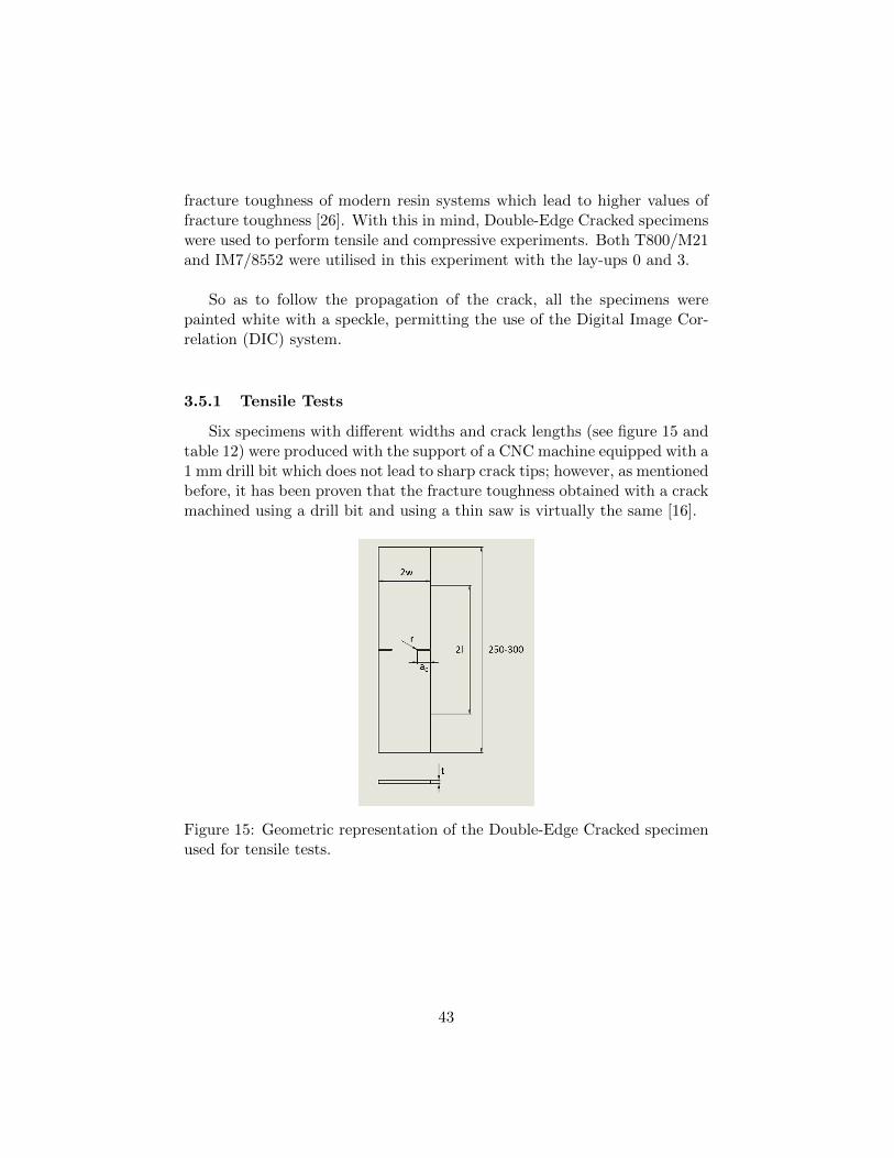
Six specimens with different widths and crack lengths (see figure 15 andtable 12) were produced with the support of a CNC machine equipped with a1 mm drill bit which does not lead to sharp crack tips; however, as mentionedbefore, it has been proven that the fracture toughness obtained with a crackmachined using a drill bit and using a thin saw is virtually the same [16].
Figure 15: Geometric representation of the Double-Edge Cracked specimenused for tensile tests.
43
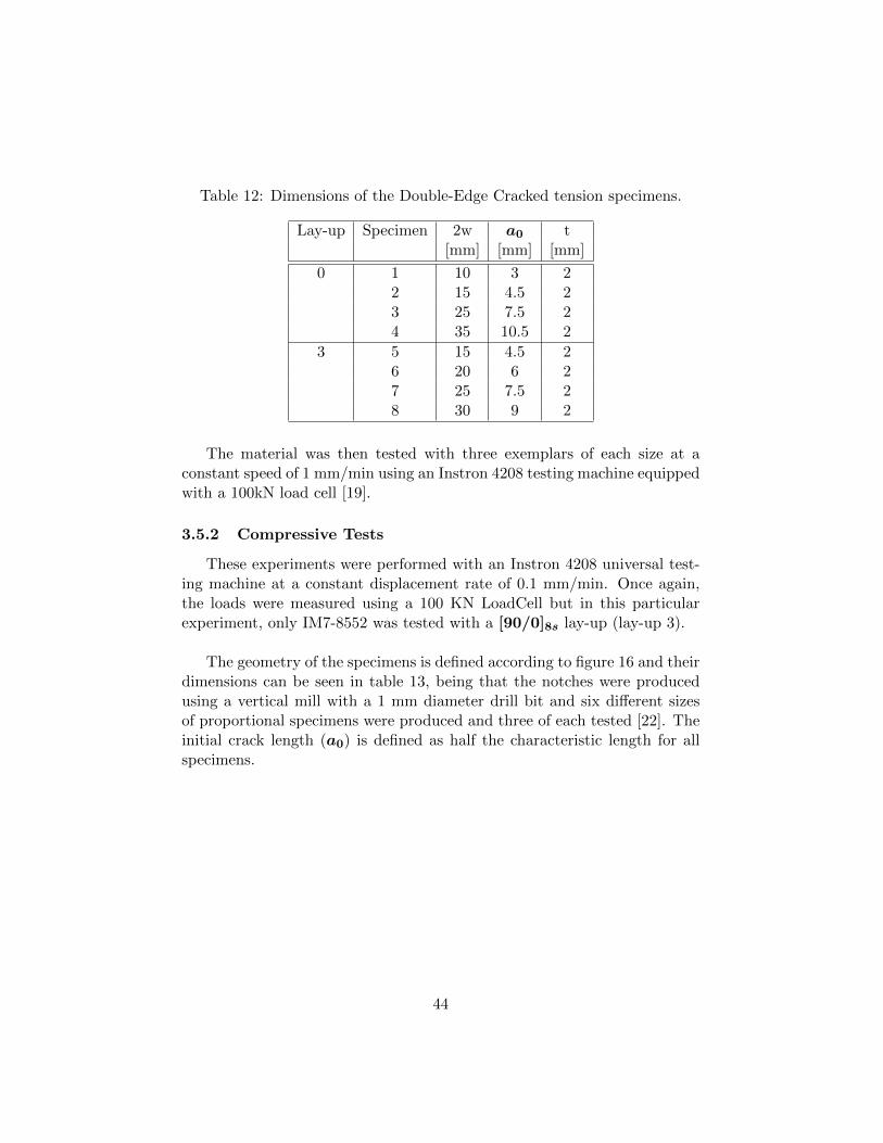
Table 12: Dimensions of the Double-Edge Cracked tension specimens.
Lay-up Specimen 2w a0 t[mm] [mm] [mm]
0 1 10 3 22 15 4.5 23 25 7.5 24 35 10.5 2
3 5 15 4.5 26 20 6 27 25 7.5 28 30 9 2
The material was then tested with three exemplars of each size at aconstant speed of 1 mm/min using an Instron 4208 testing machine equippedwith a 100kN load cell [19].
3.5.2 Compressive Tests
These experiments were performed with an Instron 4208 universal test-ing machine at a constant displacement rate of 0.1 mm/min. Once again,the loads were measured using a 100 KN LoadCell but in this particularexperiment, only IM7-8552 was tested with a [90/0]8s lay-up (lay-up 3).
The geometry of the specimens is defined according to figure 16 and theirdimensions can be seen in table 13, being that the notches were producedusing a vertical mill with a 1 mm diameter drill bit and six different sizesof proportional specimens were produced and three of each tested [22]. Theinitial crack length (a0) is defined as half the characteristic length for allspecimens.
44
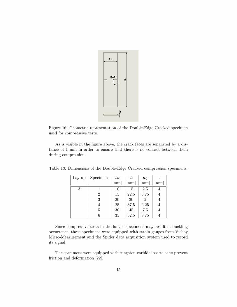
Figure 16: Geometric representation of the Double-Edge Cracked specimenused for compressive tests.
As is visible in the figure above, the crack faces are separated by a dis-tance of 1 mm in order to ensure that there is no contact between themduring compression.
Table 13: Dimensions of the Double-Edge Cracked compression specimens.
Lay-up Specimen 2w 2l a0 t[mm] [mm] [mm] [mm]
3 1 10 15 2.5 42 15 22.5 3.75 43 20 30 5 44 25 37.5 6.25 45 30 45 7.5 46 35 52.5 8.75 4
Since compressive tests in the longer specimens may result in bucklingoccurrence, these specimens were equipped with strain gauges from VishayMicro-Measurement and the Spider data acquisition system used to recordits signal.
The specimens were equipped with tungsten-carbide inserts as to preventfriction and deformation [22].
45
3.5.3 Experimental results for the Double-Edge Cracked speci-mens
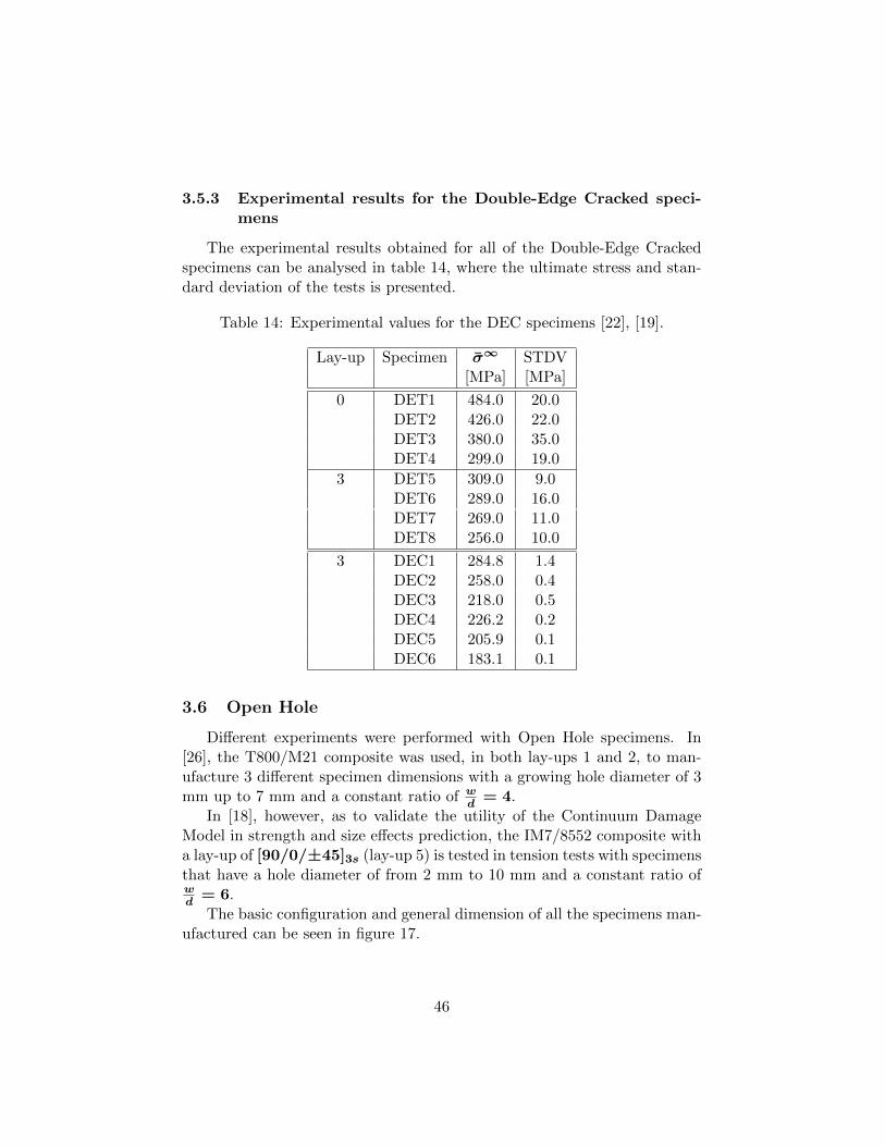
The experimental results obtained for all of the Double-Edge Crackedspecimens can be analysed in table 14, where the ultimate stress and stan-dard deviation of the tests is presented.
Table 14: Experimental values for the DEC specimens [22], [19].
Lay-up Specimen σ∞ STDV[MPa] [MPa]
0 DET1 484.0 20.0DET2 426.0 22.0DET3 380.0 35.0DET4 299.0 19.0
3 DET5 309.0 9.0DET6 289.0 16.0DET7 269.0 11.0DET8 256.0 10.0
3 DEC1 284.8 1.4DEC2 258.0 0.4DEC3 218.0 0.5DEC4 226.2 0.2DEC5 205.9 0.1DEC6 183.1 0.1
3.6 Open Hole
Different experiments were performed with Open Hole specimens. In[26], the T800/M21 composite was used, in both lay-ups 1 and 2, to man-ufacture 3 different specimen dimensions with a growing hole diameter of 3mm up to 7 mm and a constant ratio of w
d= 4.
In [18], however, as to validate the utility of the Continuum DamageModel in strength and size effects prediction, the IM7/8552 composite witha lay-up of [90/0/±45]3s (lay-up 5) is tested in tension tests with specimensthat have a hole diameter of from 2 mm to 10 mm and a constant ratio ofwd
= 6.The basic configuration and general dimension of all the specimens man-
ufactured can be seen in figure 17.
46
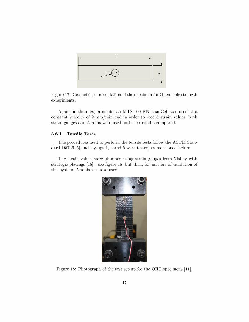
Figure 17: Geometric representation of the specimen for Open Hole strengthexperiments.
Again, in these experiments, an MTS-100 KN LoadCell was used at aconstant velocity of 2 mm/min and in order to record strain values, bothstrain gauges and Aramis were used and their results compared.
3.6.1 Tensile Tests
The procedures used to perform the tensile tests follow the ASTM Stan-dard D5766 [5] and lay-ups 1, 2 and 5 were tested, as mentioned before.
The strain values were obtained using strain gauges from Vishay withstrategic placings [18] - see figure 18, but then, for matters of validation ofthis system, Aramis was also used.
Figure 18: Photograph of the test set-up for the OHT specimens [11].
47
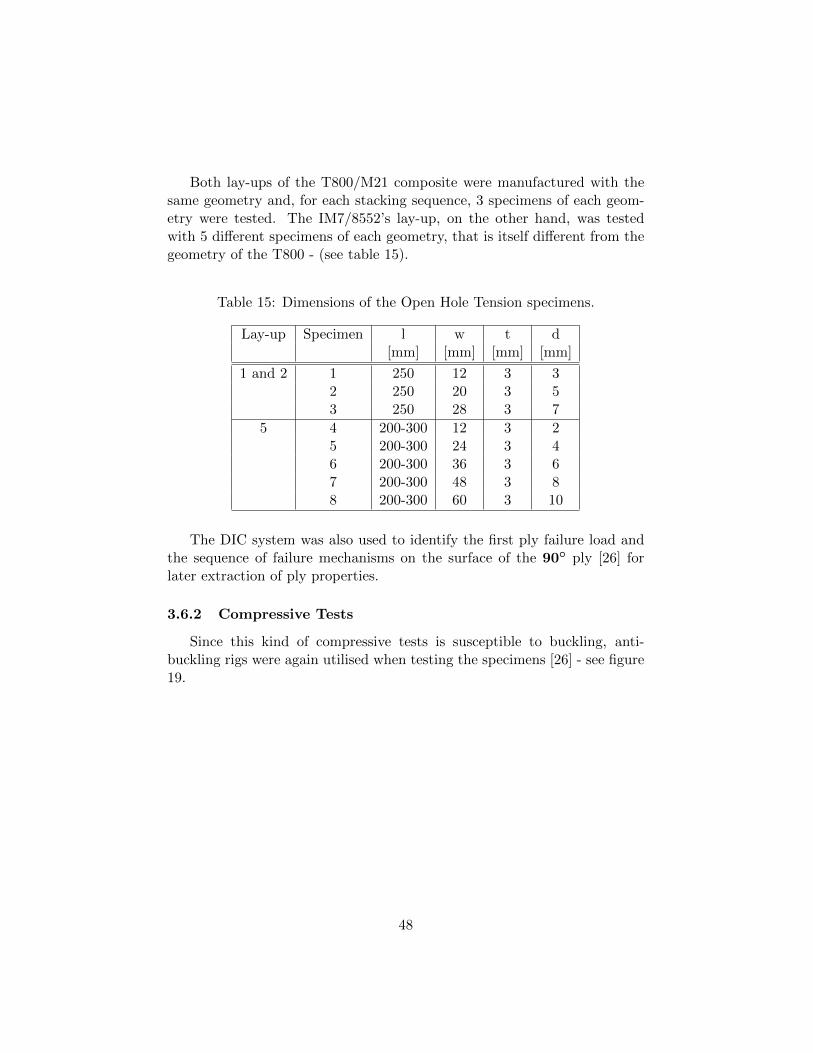
Both lay-ups of the T800/M21 composite were manufactured with thesame geometry and, for each stacking sequence, 3 specimens of each geom-etry were tested. The IM7/8552’s lay-up, on the other hand, was testedwith 5 different specimens of each geometry, that is itself different from thegeometry of the T800 - (see table 15).
Table 15: Dimensions of the Open Hole Tension specimens.
Lay-up Specimen l w t d[mm] [mm] [mm] [mm]
1 and 2 1 250 12 3 32 250 20 3 53 250 28 3 7
5 4 200-300 12 3 25 200-300 24 3 46 200-300 36 3 67 200-300 48 3 88 200-300 60 3 10
The DIC system was also used to identify the first ply failure load andthe sequence of failure mechanisms on the surface of the 90◦ ply [26] forlater extraction of ply properties.
3.6.2 Compressive Tests
Since this kind of compressive tests is susceptible to buckling, anti-buckling rigs were again utilised when testing the specimens [26] - see figure19.
48
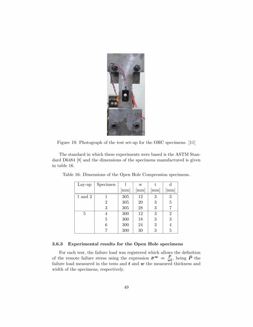
Figure 19: Photograph of the test set-up for the OHC specimens. [11]
The standard in which these experiments were based is the ASTM Stan-dard D6484 [8] and the dimensions of the specimens manufactured is givenin table 16.
Table 16: Dimensions of the Open Hole Compression specimens.
Lay-up Specimen l w t d[mm] [mm] [mm] [mm]
1 and 2 1 305 12 3 32 305 20 3 53 305 28 3 7
5 4 300 12 3 25 300 18 3 36 300 24 3 47 300 30 3 5
3.6.3 Experimental results for the Open Hole specimens
For each test, the failure load was registered which allows the definitionof the remote failure stress using the expression σ∞ = P
wt, being P the
failure load measured in the tests and t and w the measured thickness andwidth of the specimens, respectively.
49
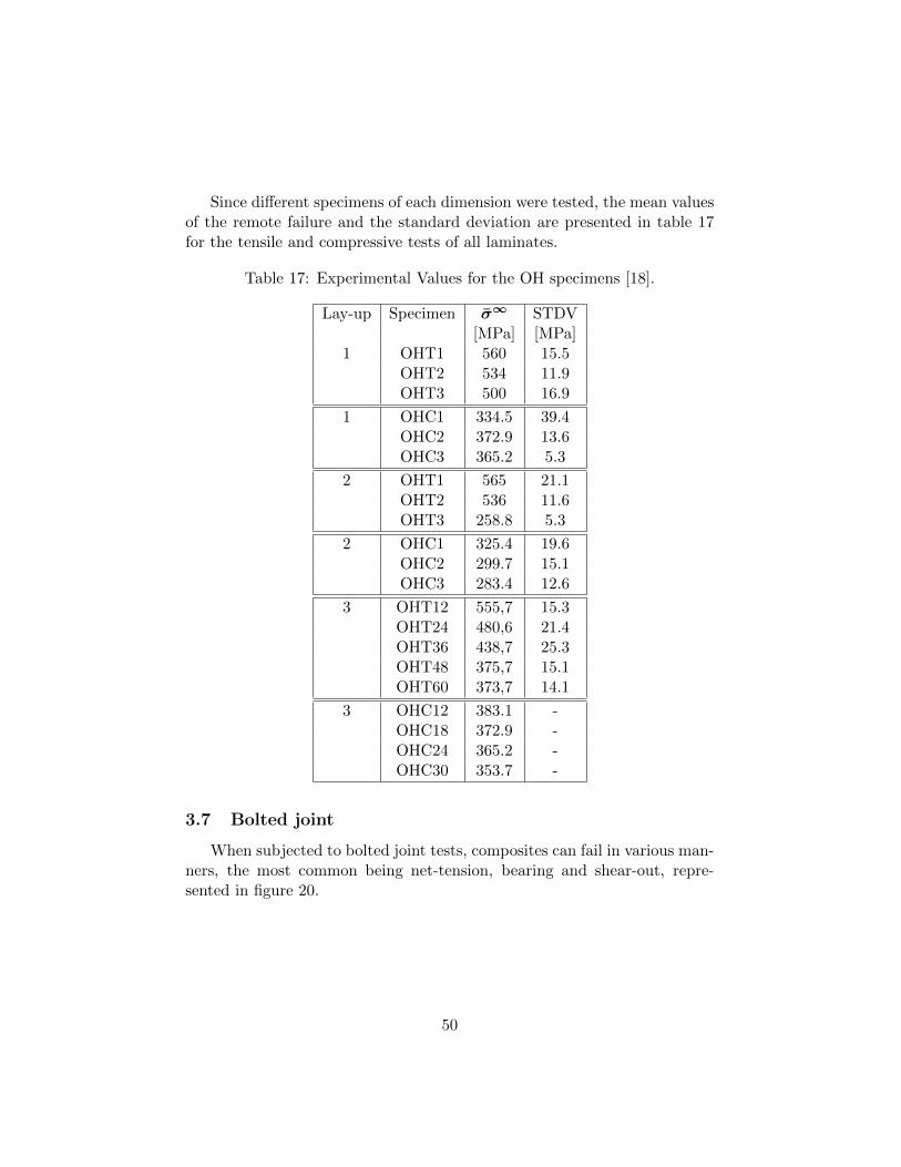
Since different specimens of each dimension were tested, the mean valuesof the remote failure and the standard deviation are presented in table 17for the tensile and compressive tests of all laminates.
Table 17: Experimental Values for the OH specimens [18].
Lay-up Specimen σ∞ STDV[MPa] [MPa]
1 OHT1 560 15.5OHT2 534 11.9OHT3 500 16.9
1 OHC1 334.5 39.4OHC2 372.9 13.6OHC3 365.2 5.3
2 OHT1 565 21.1OHT2 536 11.6OHT3 258.8 5.3
2 OHC1 325.4 19.6OHC2 299.7 15.1OHC3 283.4 12.6
3 OHT12 555,7 15.3OHT24 480,6 21.4OHT36 438,7 25.3OHT48 375,7 15.1OHT60 373,7 14.1
3 OHC12 383.1 -OHC18 372.9 -OHC24 365.2 -OHC30 353.7 -
3.7 Bolted joint
When subjected to bolted joint tests, composites can fail in various man-ners, the most common being net-tension, bearing and shear-out, repre-sented in figure 20.
50
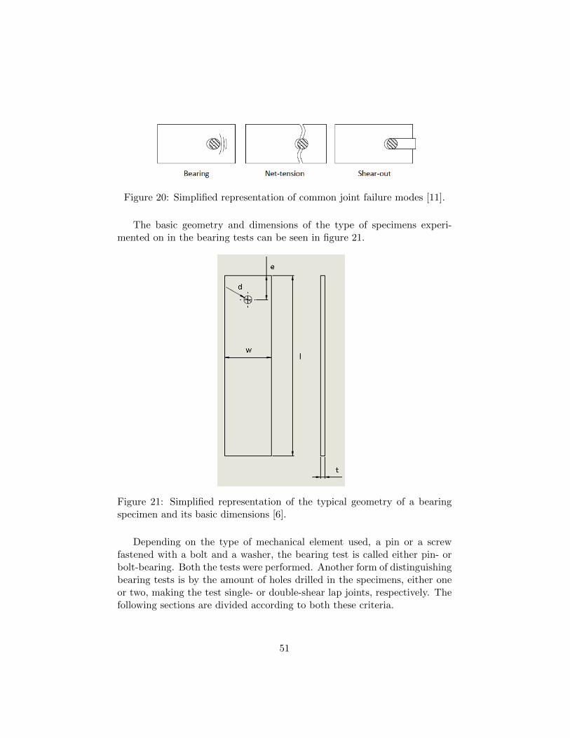
Figure 20: Simplified representation of common joint failure modes [11].
The basic geometry and dimensions of the type of specimens experi-mented on in the bearing tests can be seen in figure 21.
Figure 21: Simplified representation of the typical geometry of a bearingspecimen and its basic dimensions [6].
Depending on the type of mechanical element used, a pin or a screwfastened with a bolt and a washer, the bearing test is called either pin- orbolt-bearing. Both the tests were performed. Another form of distinguishingbearing tests is by the amount of holes drilled in the specimens, either oneor two, making the test single- or double-shear lap joints, respectively. Thefollowing sections are divided according to both these criteria.
51
3.7.1 Single-shear lap joints
3.7.1.1 Bolt-Bearing
The purpose of bolt-bearing tests is evaluating the mechanical behaviourof the thin-ply laminates when subjected to local compressive efforts, whichtypically occurs with mechanically fastened joints.
The type of failure mode described in this subsection is a non-catastrophicone that results from a progressive accumulation of damage that subse-quently results in a permanent deformation of the hole in compression. Thebolt-bearing tests were performed according to ASTM Standard D5961 [6].
In order to perform the tests, a M6 bolt is used with an applied torqueof 2.2 N.m, and then, under displacement control, in a servo-hydraulic MTS810 testing machine, one specimen per geometry was instrumented equippedwith a strain gauge in the longitudinal direction.
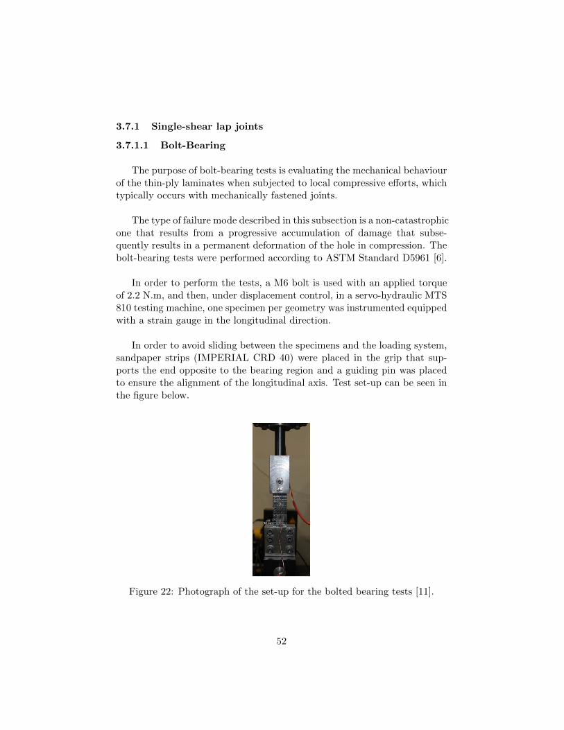
In order to avoid sliding between the specimens and the loading system,sandpaper strips (IMPERIAL CRD 40) were placed in the grip that sup-ports the end opposite to the bearing region and a guiding pin was placedto ensure the alignment of the longitudinal axis. Test set-up can be seen inthe figure below.
Figure 22: Photograph of the set-up for the bolted bearing tests [11].
52
The dimensions of the specimens used in the single bolt-bearing tests canbe seen in table 18, keeping in mind that five specimens of each dimensionwere tested. The dW that appears in the table represents the diameter ofthe washers used.
Table 18: Dimensions of the single bolt-bearing specimens.
Lay-up Specimen 2l 2w e t d dw[mm] [mm] [mm] [mm] [mm] [mm]
3 1 135 36 18 3 6 122 135 48 24 3 8 133 135 60 30 3 10 14.5
3.7.1.2 Pin-Bearing
In this test, again, the purpose is to study how the material reacts to aconnection, now with a pin. The main difference to shed light on is the factthat here no clamping pressure is applied.
The same ASTM Standard is used for these tests, the D5961 one [6],just as the same procedure is used to avoid sliding.
The specimens used in the single pin-bearing tests had a basic geometryas shown in figure 21 and their dimensions can be seen in table 19, keepingin mind, once again, that five specimens of each dimension were tested.
Table 19: Dimensions of the single pin-bearing specimens.
Lay-up Specimen 2l 2w e t d[mm] [mm] [mm] [mm] [mm]
3 1 135 36 18 3 62 135 48 24 3 83 135 60 30 3 10
3.7.2 Double-shear lap joints
Even though the specimen used in the double-shear tests is similar tothe single-shear tests, it is important to note that the distance between
53
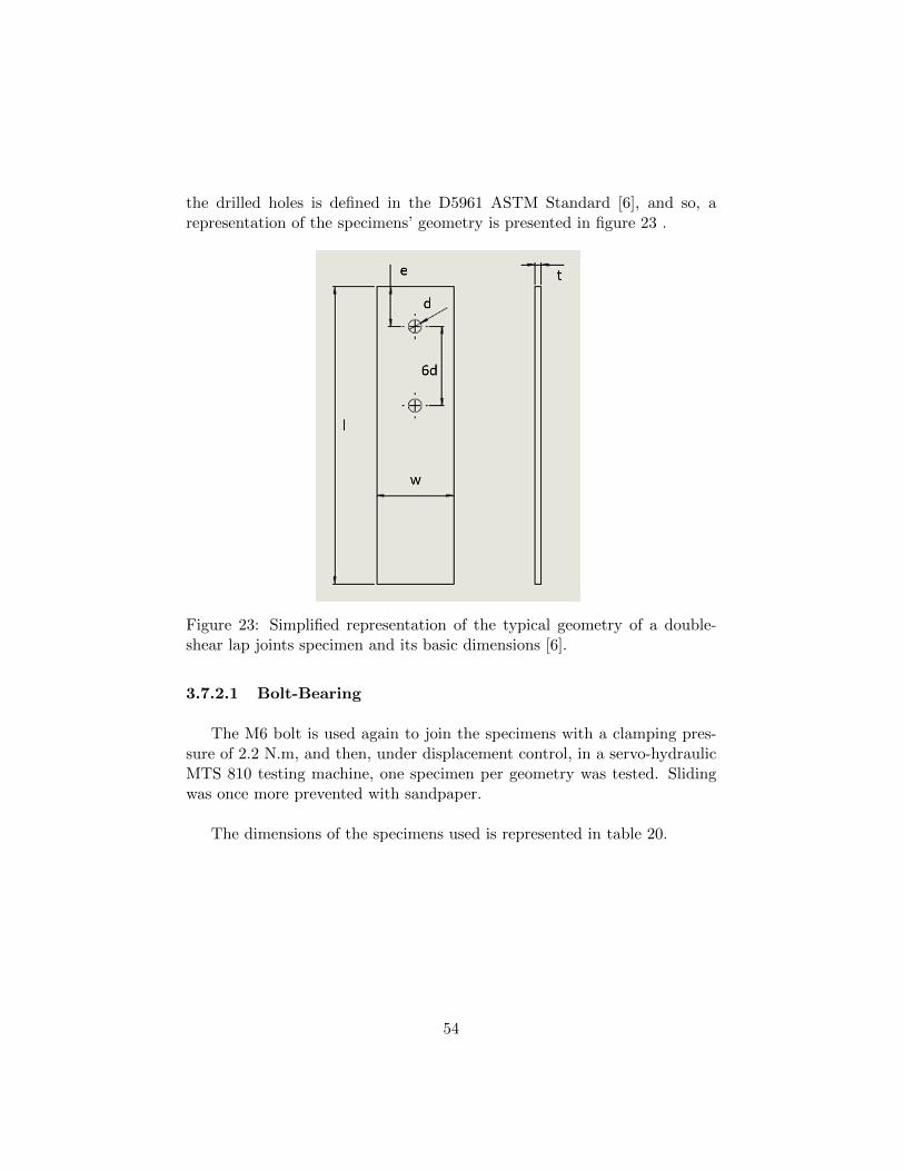
the drilled holes is defined in the D5961 ASTM Standard [6], and so, arepresentation of the specimens’ geometry is presented in figure 23 .
Figure 23: Simplified representation of the typical geometry of a double-shear lap joints specimen and its basic dimensions [6].
3.7.2.1 Bolt-Bearing
The M6 bolt is used again to join the specimens with a clamping pres-sure of 2.2 N.m, and then, under displacement control, in a servo-hydraulicMTS 810 testing machine, one specimen per geometry was tested. Slidingwas once more prevented with sandpaper.
The dimensions of the specimens used is represented in table 20.
54
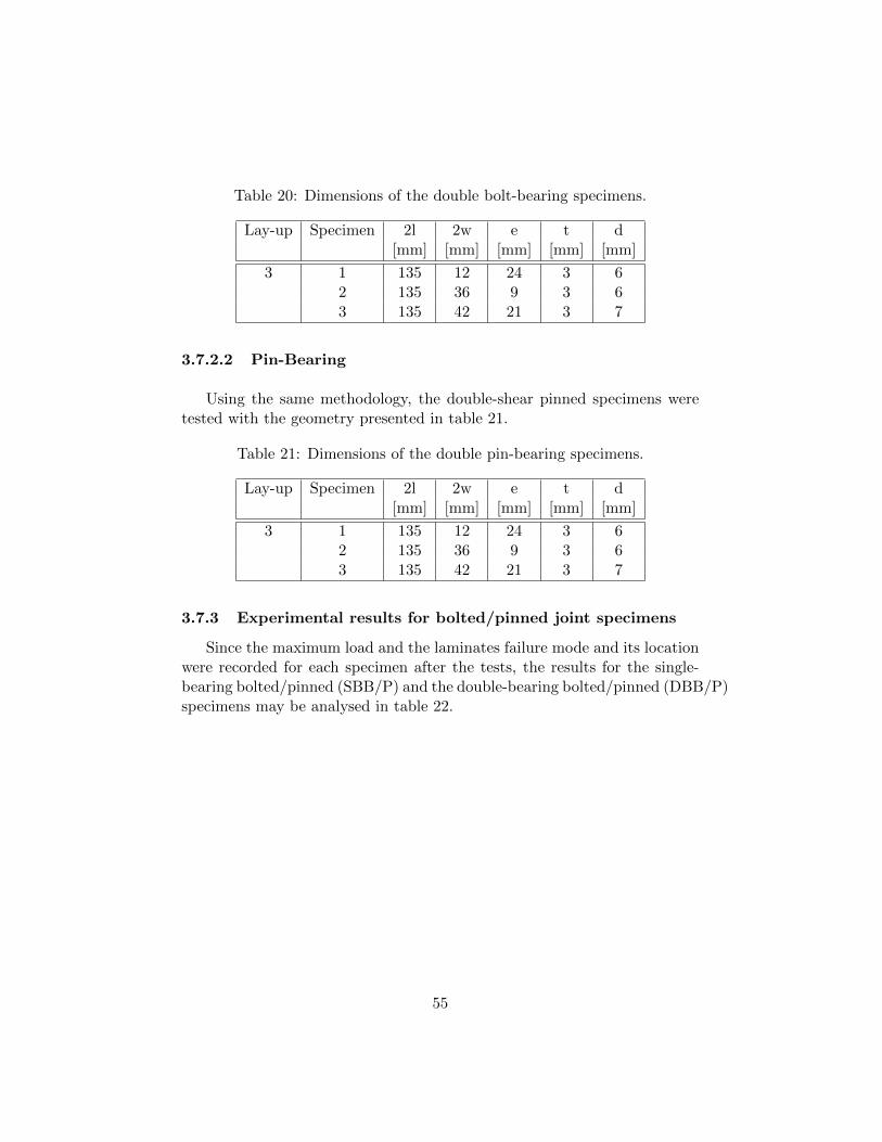
Table 20: Dimensions of the double bolt-bearing specimens.
Lay-up Specimen 2l 2w e t d[mm] [mm] [mm] [mm] [mm]
3 1 135 12 24 3 62 135 36 9 3 63 135 42 21 3 7
3.7.2.2 Pin-Bearing
Using the same methodology, the double-shear pinned specimens weretested with the geometry presented in table 21.
Table 21: Dimensions of the double pin-bearing specimens.
Lay-up Specimen 2l 2w e t d[mm] [mm] [mm] [mm] [mm]
3 1 135 12 24 3 62 135 36 9 3 63 135 42 21 3 7
3.7.3 Experimental results for bolted/pinned joint specimens
Since the maximum load and the laminates failure mode and its locationwere recorded for each specimen after the tests, the results for the single-bearing bolted/pinned (SBB/P) and the double-bearing bolted/pinned (DBB/P)specimens may be analysed in table 22.
55
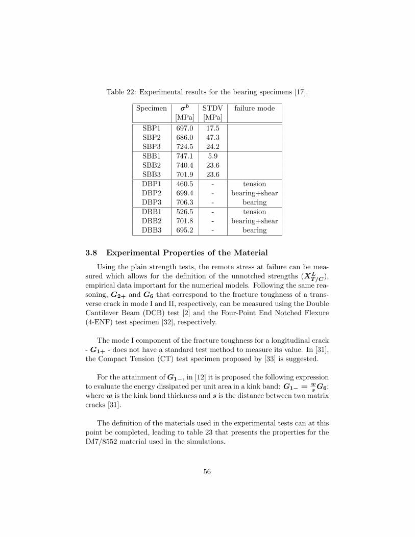
Table 22: Experimental results for the bearing specimens [17].
Specimen σb STDV failure mode[MPa] [MPa]
SBP1 697.0 17.5SBP2 686.0 47.3SBP3 724.5 24.2
SBB1 747.1 5.9SBB2 740.4 23.6SBB3 701.9 23.6
DBP1 460.5 - tensionDBP2 699.4 - bearing+shearDBP3 706.3 - bearing
DBB1 526.5 - tensionDBB2 701.8 - bearing+shearDBB3 695.2 - bearing
3.8 Experimental Properties of the Material
Using the plain strength tests, the remote stress at failure can be mea-sured which allows for the definition of the unnotched strengths (XL
T/C),empirical data important for the numerical models. Following the same rea-soning, G2+ and G6 that correspond to the fracture toughness of a trans-verse crack in mode I and II, respectively, can be measured using the DoubleCantilever Beam (DCB) test [2] and the Four-Point End Notched Flexure(4-ENF) test specimen [32], respectively.
The mode I component of the fracture toughness for a longitudinal crack- G1+ - does not have a standard test method to measure its value. In [31],the Compact Tension (CT) test specimen proposed by [33] is suggested.
For the attainment ofG1−, in [12] it is proposed the following expressionto evaluate the energy dissipated per unit area in a kink band: G1− = w
sG6;
where w is the kink band thickness and s is the distance between two matrixcracks [31].
The definition of the materials used in the experimental tests can at thispoint be completed, leading to table 23 that presents the properties for theIM7/8552 material used in the simulations.
56
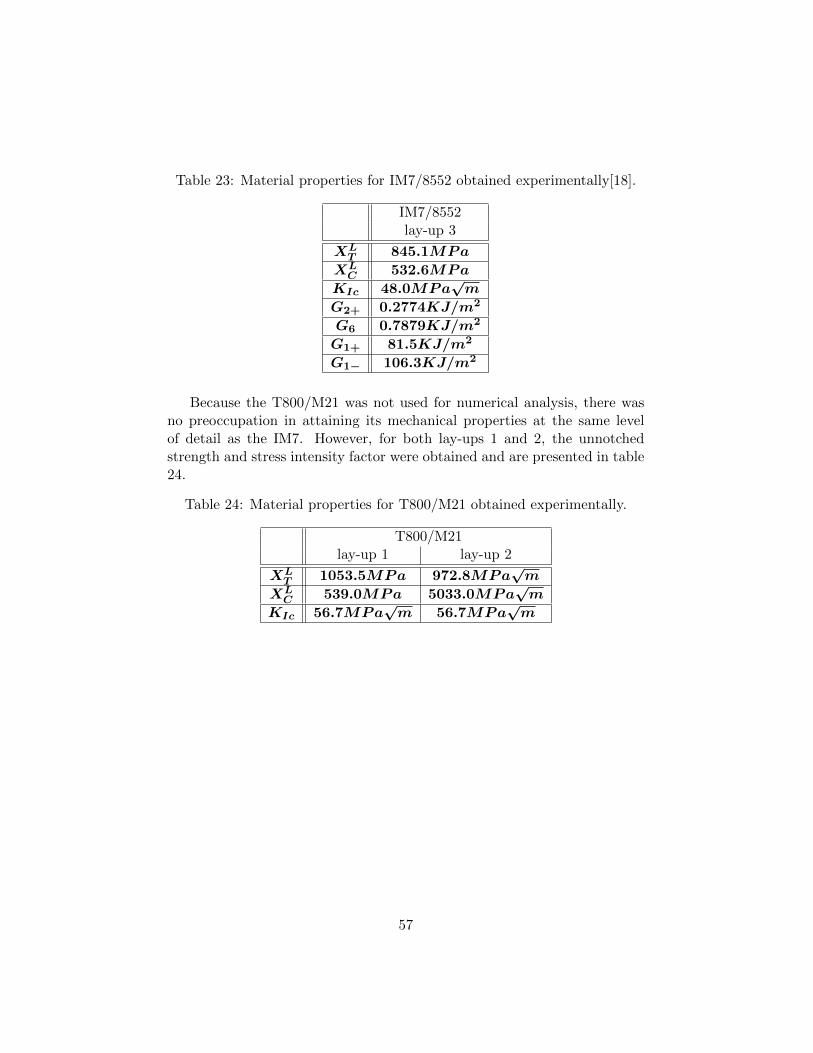
Table 23: Material properties for IM7/8552 obtained experimentally[18].
IM7/8552lay-up 3
XLT 845.1MPa
XLC 532.6MPa
KIc 48.0MPa√m
G2+ 0.2774KJ/m2
G6 0.7879KJ/m2
G1+ 81.5KJ/m2
G1− 106.3KJ/m2
Because the T800/M21 was not used for numerical analysis, there wasno preoccupation in attaining its mechanical properties at the same levelof detail as the IM7. However, for both lay-ups 1 and 2, the unnotchedstrength and stress intensity factor were obtained and are presented in table24.
Table 24: Material properties for T800/M21 obtained experimentally.
T800/M21lay-up 1 lay-up 2
XLT 1053.5MPa 972.8MPa
√m
XLC 539.0MPa 5033.0MPa
√m
KIc 56.7MPa√m 56.7MPa
√m
57
4 Prediction of damage propagation and fractureof the IM7/8552
To perform the numerical analysis of the specimens using IM7/8552CFRP in a [90, 0,±45]3s lay-up, Abaqus was used in the explicit modeto implement user subroutines.
In this chapter, the implementation of the models and criteria used in theroutines will be described bearing in mind that this method was used so asto overcome the restrictive input methods sometimes provided by Abaqus’scapabilities [25].
In order to test the various routines developed, their submission wasmade in the Avalanche Linux cluster with a 2xIntel E5-2450 CPU consist-ing of a total of 16 CPU cores, at FEUP.
4.1 Implementation
Since both non-linear behaviour and contact between plies are under re-view, the use of Abaqus/Explicit is justified for the analysis of the loadingof the increasingly complex specimens.
The following chapter is divided in 3 different parts that correlate withthe main subjects dealt with in the routines: the mesh, the surface interac-tion and the models and criteria implemented in the routines.
Quasi-static simulations are performed, which means that the velocitydefined is low and so the kinetic energy is very small relatively to the peakinternal energy. Therefore, a balance must be achieved between the qualityof the results (low relative errors) and the time spent running the routines.To do so, there was the preoccupation of analysing mass scaling and in-creasing and decreasing the amount of non-physical mass added in order toobtain a balance between quality and time management.
4.1.1 Mesh
To develop the mesh, an analysis of the different forms of constructingit was performed. A non-structured mesh could be used as described in
58
[26], for its simplicity, and, on the other hand, a structured mesh could beimplemented as well in the expectation of better results.
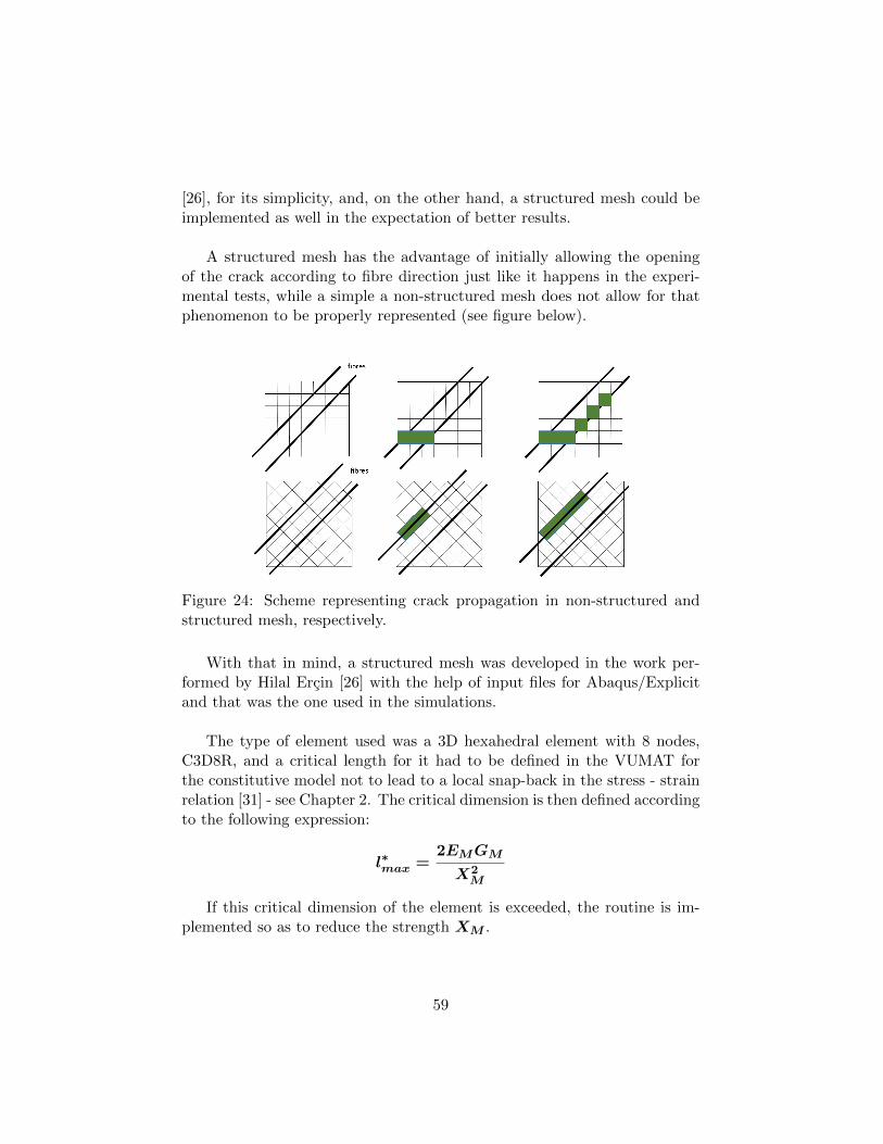
A structured mesh has the advantage of initially allowing the openingof the crack according to fibre direction just like it happens in the experi-mental tests, while a simple a non-structured mesh does not allow for thatphenomenon to be properly represented (see figure below).
Figure 24: Scheme representing crack propagation in non-structured andstructured mesh, respectively.
With that in mind, a structured mesh was developed in the work per-formed by Hilal Ercin [26] with the help of input files for Abaqus/Explicitand that was the one used in the simulations.
The type of element used was a 3D hexahedral element with 8 nodes,C3D8R, and a critical length for it had to be defined in the VUMAT forthe constitutive model not to lead to a local snap-back in the stress - strainrelation [31] - see Chapter 2. The critical dimension is then defined accordingto the following expression:
l∗max =2EMGM
X2M
If this critical dimension of the element is exceeded, the routine is im-plemented so as to reduce the strength XM .
59
Exceptionally, in the ±45 plies of the Open Hole specimens, some 6-node linear triangular prism elements had to be used so as to accommodatethe hole, despite their poor convergence rate. In this case, the first orderC3D6 element was chosen.
Since a non-linear and catastrophic analyses was performed, there wasthe concern of activating the hourglass control which prevents an excessivedistortion due to the elements instability that results from reduced integra-tion [25].
4.1.2 Cohesive behaviour
To define the relation between the lamina, cohesive surfaces where de-fined in user subroutines so as to best represent delamination. Using the sur-faces allows for the specification of generalised traction-separation behaviourbetween two adjacent surfaces. It is easier to define in multi-directional lam-inates than cohesive elements and allows the simulation of a wider range ofcohesive interactions [42].
A cohesive surface relates the loading transmitted over the surface to theseparation between the surfaces not affecting the stiffness of the material.Furthermore, during damage evolution, the ability to transmit tractions overthe cohesive surface is affected while the rest of the material remains elas-tic. Delamination thus progresses solely based on the strength degradationin the cohesive surfaces and the interaction with the elastic regions of thematerial [38].
The routines were submitted at first with Abaqus’ surface interactiondefined. However, as can be seen in [35] and [36], the software has an im-plementation error related to the B-K criterion [13] that over-predicts theanalytical results by as much as 35% [36]. However, when the B-K criterionis supplied in a user defined tabular form, the results correlate much betterwith the analytical solution [36]. That said, in an attempt to correct theerror in question, a user surface interaction was implemented in the codespecifying the Gc in tabular form as a function of the mode mixity ratio[36] - see Appendix A.
In a more technical note, an uncoupled traction-separation behaviouris defined, which means that each traction component depends only on its
60
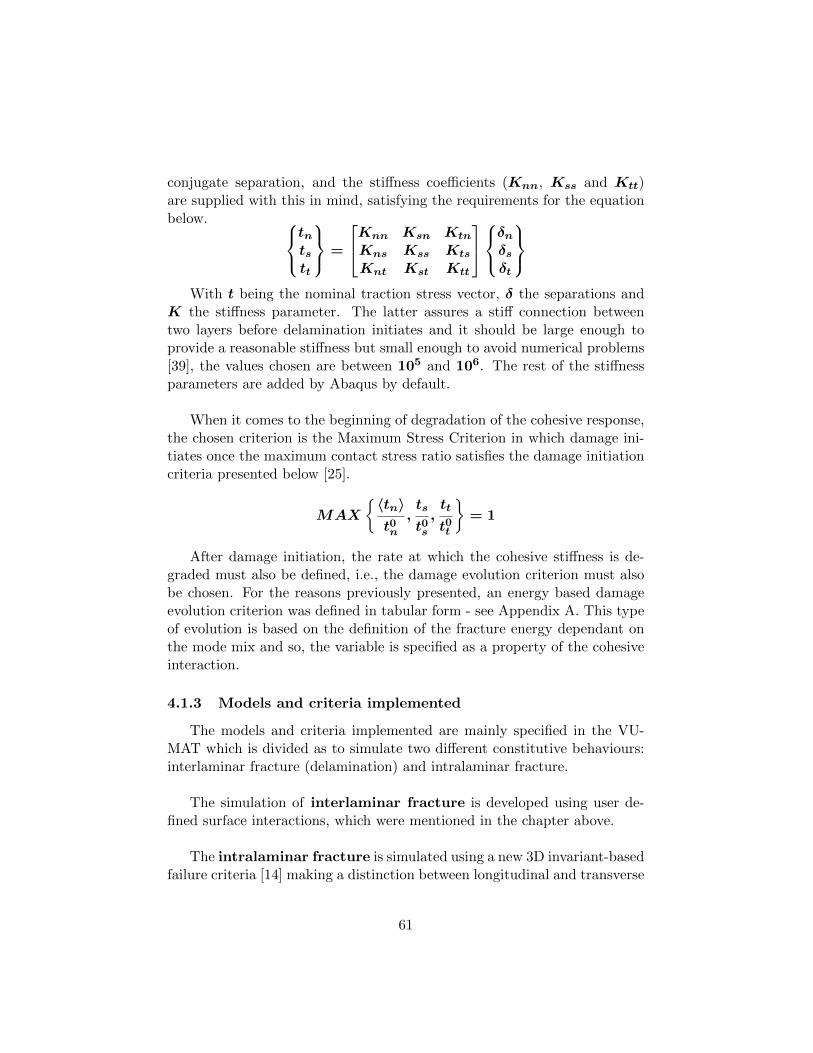
conjugate separation, and the stiffness coefficients (Knn, Kss and Ktt)are supplied with this in mind, satisfying the requirements for the equationbelow.
tntstt
=
Knn Ksn Ktn
Kns Kss Kts
Knt Kst Ktt
δnδsδt
With t being the nominal traction stress vector, δ the separations and
K the stiffness parameter. The latter assures a stiff connection betweentwo layers before delamination initiates and it should be large enough toprovide a reasonable stiffness but small enough to avoid numerical problems[39], the values chosen are between 105 and 106. The rest of the stiffnessparameters are added by Abaqus by default.
When it comes to the beginning of degradation of the cohesive response,the chosen criterion is the Maximum Stress Criterion in which damage ini-tiates once the maximum contact stress ratio satisfies the damage initiationcriteria presented below [25].
MAX
{〈tn〉t0n
,ts
t0s,tt
t0t
}= 1
After damage initiation, the rate at which the cohesive stiffness is de-graded must also be defined, i.e., the damage evolution criterion must alsobe chosen. For the reasons previously presented, an energy based damageevolution criterion was defined in tabular form - see Appendix A. This typeof evolution is based on the definition of the fracture energy dependant onthe mode mix and so, the variable is specified as a property of the cohesiveinteraction.
4.1.3 Models and criteria implemented
The models and criteria implemented are mainly specified in the VU-MAT which is divided as to simulate two different constitutive behaviours:interlaminar fracture (delamination) and intralaminar fracture.
The simulation of interlaminar fracture is developed using user de-fined surface interactions, which were mentioned in the chapter above.
The intralaminar fracture is simulated using a new 3D invariant-basedfailure criteria [14] making a distinction between longitudinal and transverse
61
failure, since the matrix-dominated failure (transverse failure) allows for theuse of the Smeared Crack Model while the fibre-dominated one (longitudinalfailure) does not. This is due to the fact that this failure mechanism consistsof the fracture of the reinforcing fibres and matrix but also of fibre-matrixdebonding and there are not yet well-established methods of characteriza-tion of the fracture toughness for fibre dominated failure mechanisms undergeneral loading conditions.
Therefore, to represent longitudinal failure mechanisms, a modificationof the Continuum Damage Model developed in[30] taking into account thein-situ strengths, i.e., the increase of the shear strength of a ply when em-bedded in a multi-directional laminate, as seen in 2.2, is used.
4.1.3.1 Failure Criteria
Analysing the failure criteria for longitudinal fracture, one must notethat tensile and compressive failure are differently predicted.
Tensile fracture in the fibre direction is predicted using the non-interactingmaximum allowable strain criterion as defined in section 2.2.2 and remem-bered below:
φ1− =ε11
εT1When it comes to longitudinal compressive failure, the mechanisms in
play are more complex and therefore, so is the criterion implemented. Asdeveloped in section 2.2.2, the 3D kinking model based on the invariantfailure criteria [14] formulated for transverse fracture, can be modified toconsider the misalignment angle, allowing for the prediction of failure thatoccurs due to the presence of local micro-structural defects that trigger akink band. The misalignment angle is calculated considering that φ0 = 0.
Transverse failure does not require any alterations of the criteria andso the 3D invariant criteria is applied directly as developed in [14] andpresented in section 2.2.1.
4.1.3.2 Damage Law
4.1.3.2.1 Longitudinal Failure
62
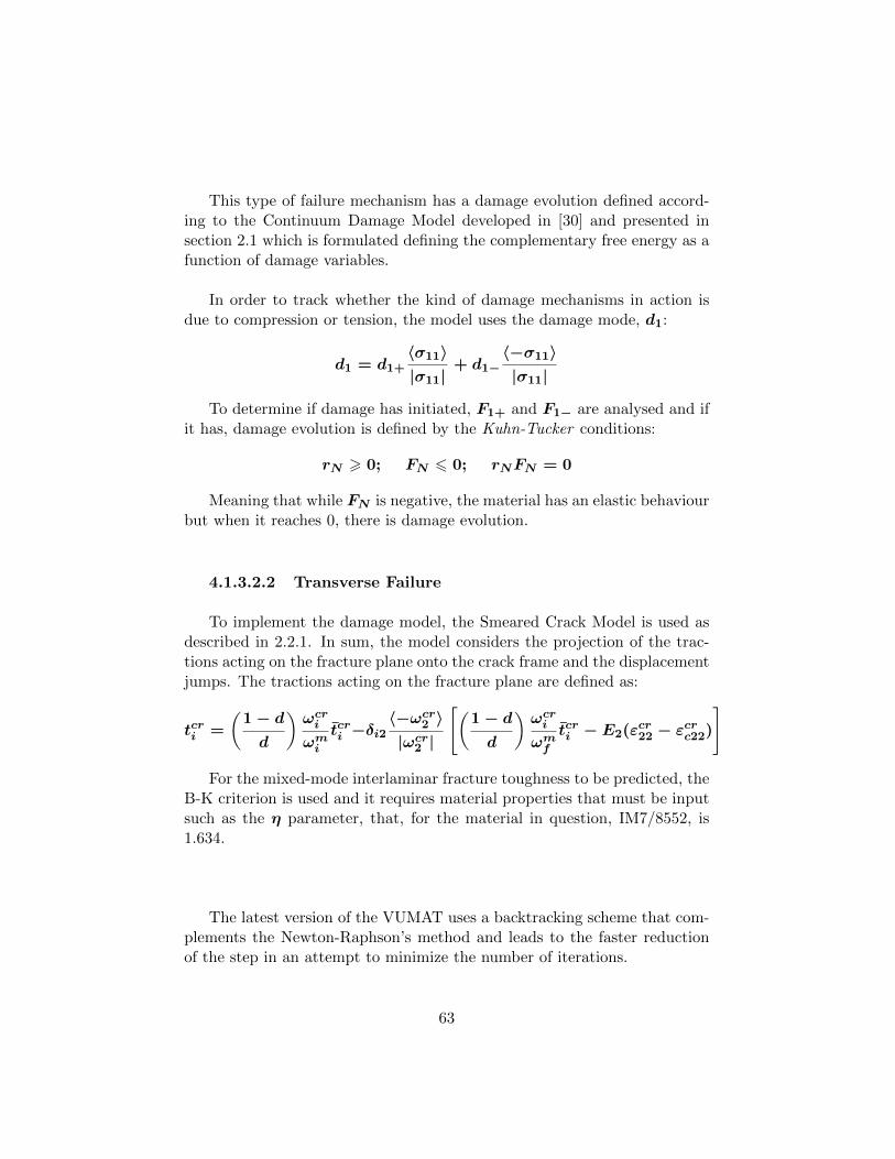
This type of failure mechanism has a damage evolution defined accord-ing to the Continuum Damage Model developed in [30] and presented insection 2.1 which is formulated defining the complementary free energy as afunction of damage variables.
In order to track whether the kind of damage mechanisms in action isdue to compression or tension, the model uses the damage mode, d1:
d1 = d1+〈σ11〉|σ11|
+ d1−〈−σ11〉|σ11|
To determine if damage has initiated, F1+ and F1− are analysed and ifit has, damage evolution is defined by the Kuhn-Tucker conditions:
rN > 0; FN 6 0; rNFN = 0
Meaning that while FN is negative, the material has an elastic behaviourbut when it reaches 0, there is damage evolution.
4.1.3.2.2 Transverse Failure
To implement the damage model, the Smeared Crack Model is used asdescribed in 2.2.1. In sum, the model considers the projection of the trac-tions acting on the fracture plane onto the crack frame and the displacementjumps. The tractions acting on the fracture plane are defined as:
tcri =
(1− dd
)ωcriωmi
tcri −δi2〈−ωcr2 〉|ωcr2 |
[(1− dd
)ωcriωmf
tcri − E2(εcr22 − εcrc22)
]
For the mixed-mode interlaminar fracture toughness to be predicted, theB-K criterion is used and it requires material properties that must be inputsuch as the η parameter, that, for the material in question, IM7/8552, is1.634.
The latest version of the VUMAT uses a backtracking scheme that com-plements the Newton-Raphson’s method and leads to the faster reductionof the step in an attempt to minimize the number of iterations.
63
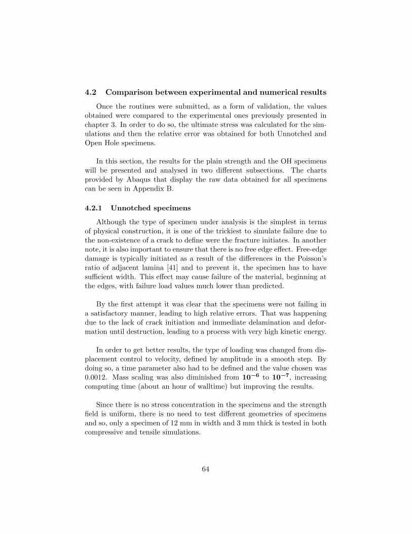
4.2 Comparison between experimental and numerical results
Once the routines were submitted, as a form of validation, the valuesobtained were compared to the experimental ones previously presented inchapter 3. In order to do so, the ultimate stress was calculated for the sim-ulations and then the relative error was obtained for both Unnotched andOpen Hole specimens.
In this section, the results for the plain strength and the OH specimenswill be presented and analysed in two different subsections. The chartsprovided by Abaqus that display the raw data obtained for all specimenscan be seen in Appendix B.
4.2.1 Unnotched specimens
Although the type of specimen under analysis is the simplest in termsof physical construction, it is one of the trickiest to simulate failure due tothe non-existence of a crack to define were the fracture initiates. In anothernote, it is also important to ensure that there is no free edge effect. Free-edgedamage is typically initiated as a result of the differences in the Poisson’sratio of adjacent lamina [41] and to prevent it, the specimen has to havesufficient width. This effect may cause failure of the material, beginning atthe edges, with failure load values much lower than predicted.
By the first attempt it was clear that the specimens were not failing ina satisfactory manner, leading to high relative errors. That was happeningdue to the lack of crack initiation and immediate delamination and defor-mation until destruction, leading to a process with very high kinetic energy.
In order to get better results, the type of loading was changed from dis-placement control to velocity, defined by amplitude in a smooth step. Bydoing so, a time parameter also had to be defined and the value chosen was0.0012. Mass scaling was also diminished from 10−6 to 10−7, increasingcomputing time (about an hour of walltime) but improving the results.
Since there is no stress concentration in the specimens and the strengthfield is uniform, there is no need to test different geometries of specimensand so, only a specimen of 12 mm in width and 3 mm thick is tested in bothcompressive and tensile simulations.
64
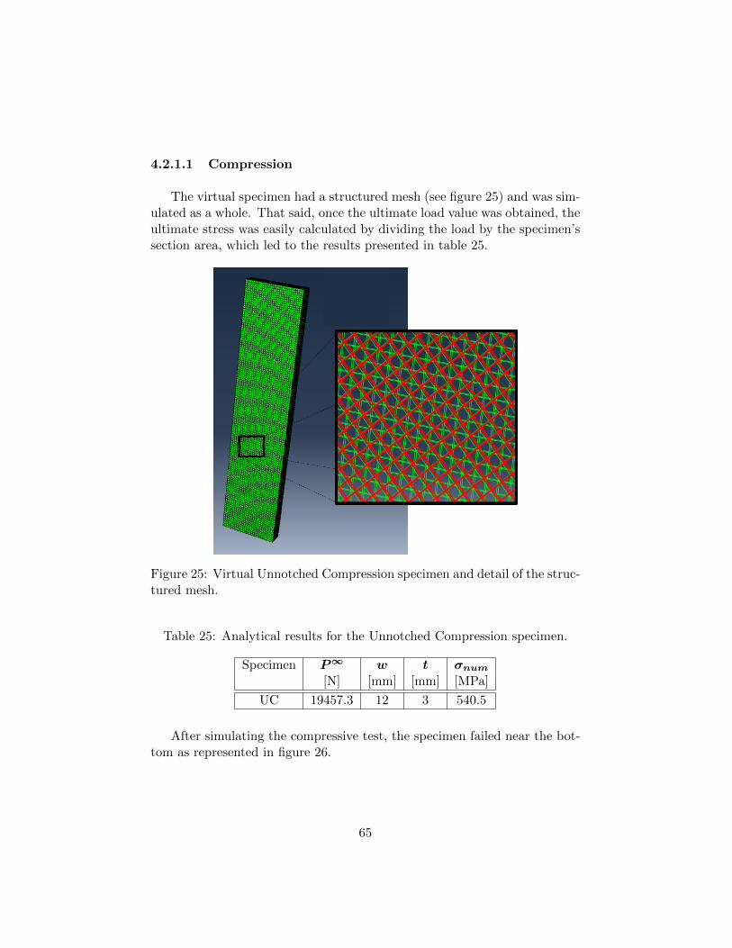
4.2.1.1 Compression
The virtual specimen had a structured mesh (see figure 25) and was sim-ulated as a whole. That said, once the ultimate load value was obtained, theultimate stress was easily calculated by dividing the load by the specimen’ssection area, which led to the results presented in table 25.
Figure 25: Virtual Unnotched Compression specimen and detail of the struc-tured mesh.
Table 25: Analytical results for the Unnotched Compression specimen.
Specimen P∞ w t σnum[N] [mm] [mm] [MPa]
UC 19457.3 12 3 540.5
After simulating the compressive test, the specimen failed near the bot-tom as represented in figure 26.
65
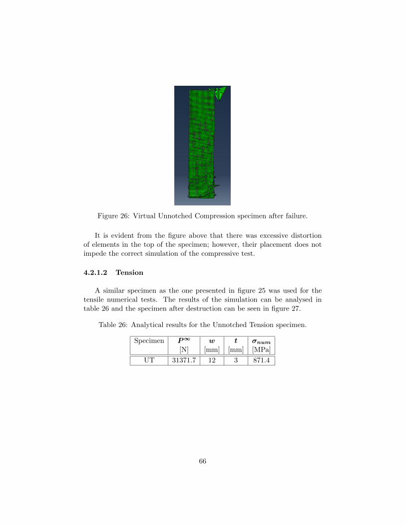
Figure 26: Virtual Unnotched Compression specimen after failure.
It is evident from the figure above that there was excessive distortionof elements in the top of the specimen; however, their placement does notimpede the correct simulation of the compressive test.
4.2.1.2 Tension
A similar specimen as the one presented in figure 25 was used for thetensile numerical tests. The results of the simulation can be analysed intable 26 and the specimen after destruction can be seen in figure 27.
Table 26: Analytical results for the Unnotched Tension specimen.
Specimen P∞ w t σnum[N] [mm] [mm] [MPa]
UT 31371.7 12 3 871.4
66
Figure 27: Virtual Unnotched Tension specimen after failure.
It is evident from the figure presented above that some elements sufferedexcessive distortion; however, the crack initiated and propagated in the bot-tom, where the elements deform as intended.
After both simulations reached the desirable results, the comparison be-tween numerical and experimental values was done by confronting both ul-timate stresses and calculating the resulting relative error, as presented inthe table below.
Table 27: Comparison between numerical and experimental values for theunnotched specimens.
Specimen P∞ σnum σexp relative error[N] [MPa] [MPa] [%]
UT 31371.7 871.4 846.1 3.0UC 19457.3 540.5 532.6 1.5
A graphical representation of the obtained results is presented in thescatter chart below.
67
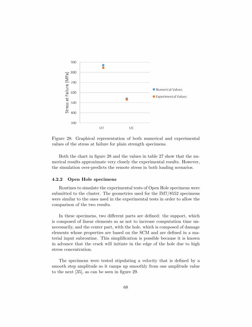
Figure 28: Graphical representation of both numerical and experimentalvalues of the stress at failure for plain strength specimens.
Both the chart in figure 28 and the values in table 27 show that the nu-merical results approximate very closely the experimental results. However,the simulation over-predicts the remote stress in both loading scenarios.
4.2.2 Open Hole specimens
Routines to simulate the experimental tests of Open Hole specimens weresubmitted to the cluster. The geometries used for the IM7/8552 specimenswere similar to the ones used in the experimental tests in order to allow thecomparison of the two results.
In these specimens, two different parts are defined: the support, whichis composed of linear elements so as not to increase computation time un-necessarily, and the center part, with the hole, which is composed of damageelements whose properties are based on the SCM and are defined in a ma-terial input subroutine. This simplification is possible because it is knownin advance that the crack will initiate in the edge of the hole due to highstress concentration.
The specimens were tested stipulating a velocity that is defined by asmooth step amplitude so it ramps up smoothly from one amplitude valueto the next [35], as can be seen in figure 29.
68
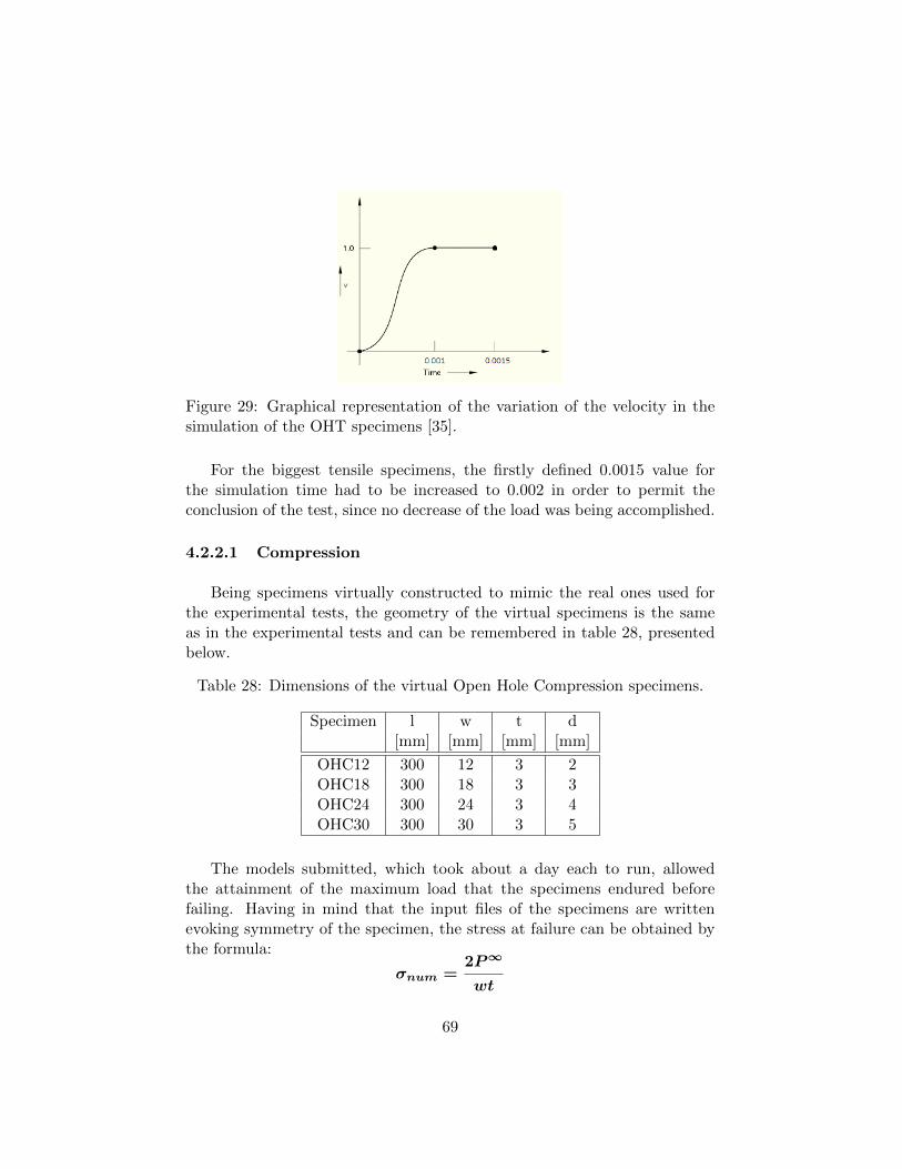
Figure 29: Graphical representation of the variation of the velocity in thesimulation of the OHT specimens [35].
For the biggest tensile specimens, the firstly defined 0.0015 value forthe simulation time had to be increased to 0.002 in order to permit theconclusion of the test, since no decrease of the load was being accomplished.
4.2.2.1 Compression
Being specimens virtually constructed to mimic the real ones used forthe experimental tests, the geometry of the virtual specimens is the sameas in the experimental tests and can be remembered in table 28, presentedbelow.
Table 28: Dimensions of the virtual Open Hole Compression specimens.
Specimen l w t d[mm] [mm] [mm] [mm]
OHC12 300 12 3 2OHC18 300 18 3 3OHC24 300 24 3 4OHC30 300 30 3 5
The models submitted, which took about a day each to run, allowedthe attainment of the maximum load that the specimens endured beforefailing. Having in mind that the input files of the specimens are writtenevoking symmetry of the specimen, the stress at failure can be obtained bythe formula:
σnum =2P∞
wt
69
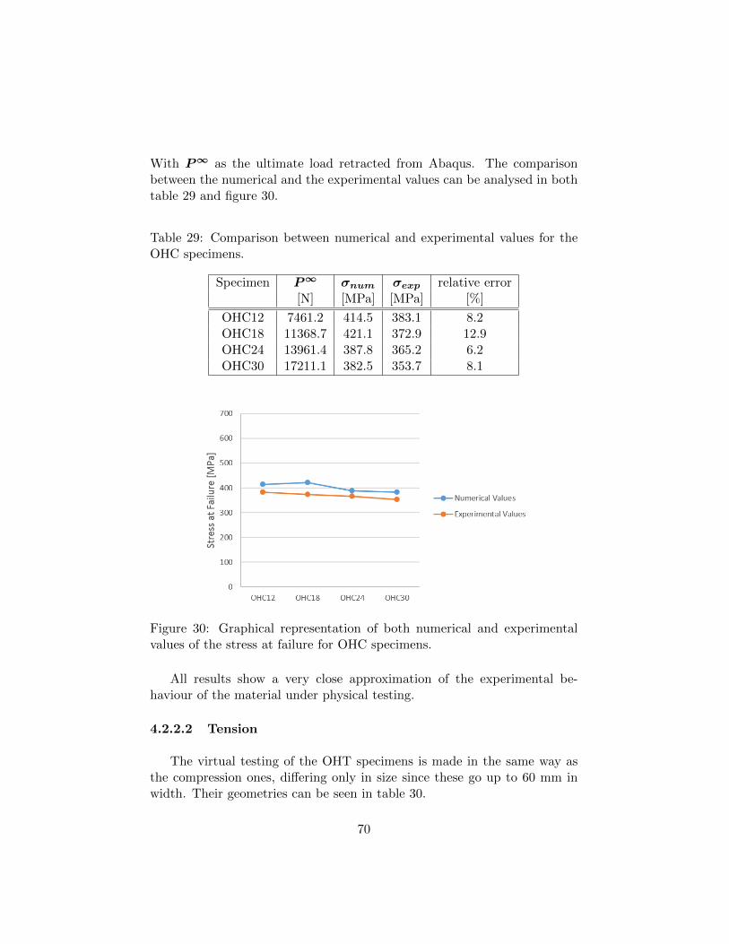
With P∞ as the ultimate load retracted from Abaqus. The comparisonbetween the numerical and the experimental values can be analysed in bothtable 29 and figure 30.
Table 29: Comparison between numerical and experimental values for theOHC specimens.
Specimen P∞ σnum σexp relative error[N] [MPa] [MPa] [%]
OHC12 7461.2 414.5 383.1 8.2OHC18 11368.7 421.1 372.9 12.9OHC24 13961.4 387.8 365.2 6.2OHC30 17211.1 382.5 353.7 8.1
Figure 30: Graphical representation of both numerical and experimentalvalues of the stress at failure for OHC specimens.
All results show a very close approximation of the experimental be-haviour of the material under physical testing.
4.2.2.2 Tension
The virtual testing of the OHT specimens is made in the same way asthe compression ones, differing only in size since these go up to 60 mm inwidth. Their geometries can be seen in table 30.
70
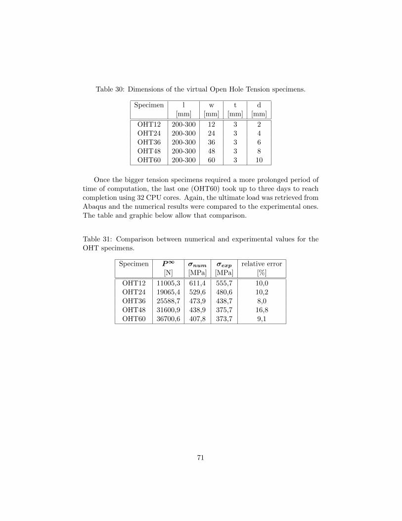
Table 30: Dimensions of the virtual Open Hole Tension specimens.
Specimen l w t d[mm] [mm] [mm] [mm]
OHT12 200-300 12 3 2OHT24 200-300 24 3 4OHT36 200-300 36 3 6OHT48 200-300 48 3 8OHT60 200-300 60 3 10
Once the bigger tension specimens required a more prolonged period oftime of computation, the last one (OHT60) took up to three days to reachcompletion using 32 CPU cores. Again, the ultimate load was retrieved fromAbaqus and the numerical results were compared to the experimental ones.The table and graphic below allow that comparison.
Table 31: Comparison between numerical and experimental values for theOHT specimens.
Specimen P∞ σnum σexp relative error[N] [MPa] [MPa] [%]
OHT12 11005,3 611,4 555,7 10,0OHT24 19065,4 529,6 480,6 10,2OHT36 25588,7 473,9 438,7 8,0OHT48 31600,9 438,9 375,7 16,8OHT60 36700,6 407,8 373,7 9,1
71
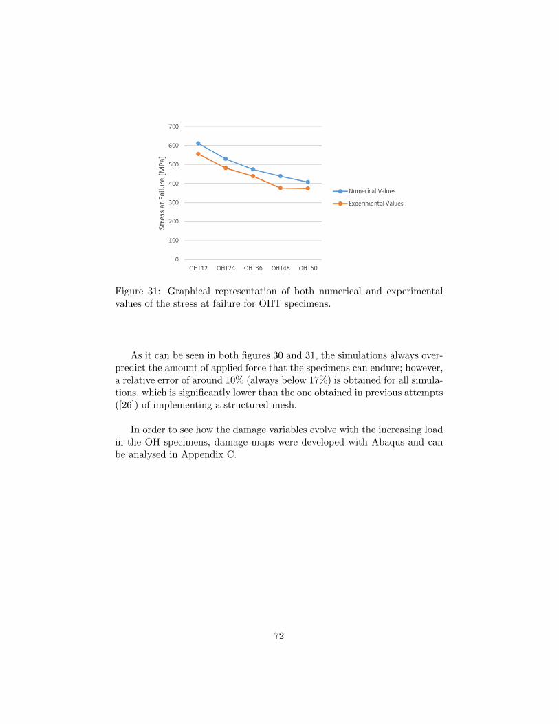
Figure 31: Graphical representation of both numerical and experimentalvalues of the stress at failure for OHT specimens.
As it can be seen in both figures 30 and 31, the simulations always over-predict the amount of applied force that the specimens can endure; however,a relative error of around 10% (always below 17%) is obtained for all simula-tions, which is significantly lower than the one obtained in previous attempts([26]) of implementing a structured mesh.
In order to see how the damage variables evolve with the increasing loadin the OH specimens, damage maps were developed with Abaqus and canbe analysed in Appendix C.
72
5 Conclusions and Future Work
In the following subsections, the conclusions that can be drawn from thedeveloped work and the improvements that can be performed in the futureas a continuation of the work developed in the present thesis are presented.
5.1 Conclusions
The main conclusions of the paper are divided as presented:
• The improvements performed to the VUMAT routine since [26] haveallowed for an average of 15% improvement in the Open Hole simu-lations; the main alterations to emphasise are in the addition of therecently developed Invariant Failure Criteria [14];
• The unnotched specimens resulted in very low relative errors, 3% forthe tensile test and 1.5% for the compressive one;
• Changing the velocity, time and mass scaling parameters of the simu-lation allows for the fine tuning of the routines and can be balanced tofind the optimal results without greatly increasing computation time;
• For the Open Hole Compression specimens, a decreasing value of theultimate stress is obtained when the hole diameter increases, eventhough w
dis kept constant at 6, which is in agreement with the ex-
perimental results. The only discrepancy is found with the Open HoleCompression (OHC18) specimen that shows a slight increase in stressfrom the specimen in the level behind it; however, even in the experi-mental tests, the decreasing tendency is of small magnitude;
• The largest OHT specimens took a very long time to simulate, whencompared to the smaller ones or the compression ones, a fact that caneasily be explained by the increase in the number of elements fromaround 30 000 to 800 000; to be noted that, already, only half of thespecimen was simulated in an effort to reduce computational time;
• In all of the OHC simulations, the specimens presented at least anelement with excessive distortion while in the tensile tests, only thebiggest specimen (w=60 mm) presented excessive distortion; it is visi-ble from the damage figures that the compressive tests are much moredestructive;
73
• Even tough the loading of the unnotched specimens may seem verystraightforward, the lack of crack or notch leads to a very unpredictablefailure behaviour.
5.2 Future Work
The future work recommended is:
• Continuation of the validation of the rest of the developed routineswith the help of the enumerated experimental tests already performed;
• To make sure that the crack in the unnotched specimens initiates inthe middle of the specimen, the .inp file could be altered in order todevelop the part with three different components: the supports withelements with an elastic behaviour and the centre of the specimenwith elements whose behaviour are based in the models presented inthe thesis;
• Test unnotched specimens with an off-axis loading and study the effectof fibre direction simulated in the structured mesh;
• Submit again the OHC18 routine, in an attempt to capture the scalelaw, after rearranging the pertinent parameters;
• In an attempt to minimize the relative error, OHT48 could be testedagain after adjusting the mass scaling and velocity parameters.
74
Appendix A
Damage Evolution Criterion in tabular form
*Damage Evolution, type=ENERGY, mixed mode behavior=TABULAR,mode mix ratio=TRACTION 0.28,0,00.280000832,0.006430284,00.280006394,0.012990437,00.28002133,0.019682997,00.280050567,0.026510489,00.280099413,0.033475417,00.280173611,0.040580253,00.280279381,0.047827433,00.280423451,0.055219341,00.280613089,0.062758304,00.280856131,0.070446575,00.281160997,0.078286324,00.281536717,0.086279622,00.28199294,0.094428432,00.282539949,0.102734586,00.28318866,0.111199776,00.283950624,0.119825532,00.284838013,0.128613209,00.285863608,0.137563966,00.287040764,0.146678746,00.288383382,0.155958261,00.28990585,0.165402965,00.291622991,0.175013041,00.293549983,0.184788375,00.295702275,0.194728537,00.298095483,0.204832765,00.300745276,0.215099935,00.303667242,0.225528553,00.306876746,0.236116728,00.310388768,0.246862159,00.314217732,0.257762117,00.318377325,0.268813433,00.3228803,0.280012485,00.327738279,0.291355186,00.332961549,0.302836982,00.338558855,0.314452842,0
75
0.344537197,0.326197262,00.350901635,0.338064264,00.357655105,0.350047408,00.364798245,0.362139794,00.372329249,0.374334084,00.38024374,0.386622514,00.388534671,0.398996923,00.397192263,0.411448773,00.406203975,0.423969184,00.415554509,0.436548965,00.425225865,0.449178653,00.435197425,0.461848552,00.445446087,0.474548777,00.455946431,0.487269302,00.466670926,0.5,00.477590172,0.512730698,00.488673167,0.525451223,00.499887603,0.538151448,00.511200177,0.550821347,00.52257692,0.563451035,00.533983527,0.576030816,00.545385691,0.588551227,00.556749429,0.601003077,00.568041398,0.613377486,00.579229188,0.625665916,00.590281601,0.637860206,00.601168896,0.649952592,00.611863007,0.661935736,00.622337732,0.673802738,00.632568885,0.685547158,00.642534412,0.697163018,00.65221448,0.708644814,00.661591529,0.719987515,00.670650291,0.731186567,00.679377783,0.742237883,00.687763274,0.753137841,00.695798229,0.763883272,00.703476222,0.774471447,00.710792853,0.784900065,00.717745626,0.795167235,0
76
0.724333834,0.805271463,00.73055843,0.815211625,00.73642189,0.824986959,00.741928074,0.834597035,00.74708209,0.844041739,00.751890156,0.853321254,00.756359466,0.862436034,00.760498057,0.871386791,00.764314689,0.880174468,00.767818723,0.888800224,00.771020015,0.897265414,00.773928808,0.905571568,00.776555638,0.913720378,00.778911248,0.921713676,00.781006508,0.929553425,00.782852342,0.937241696,00.784459665,0.944780659,00.785839328,0.952172567,00.787002065,0.959419747,00.787958453,0.966524583,00.788718871,0.973489511,00.789293473,0.980317003,00.78969216,0.987009563,00.789924558,0.993569716,00.79,1,0
77
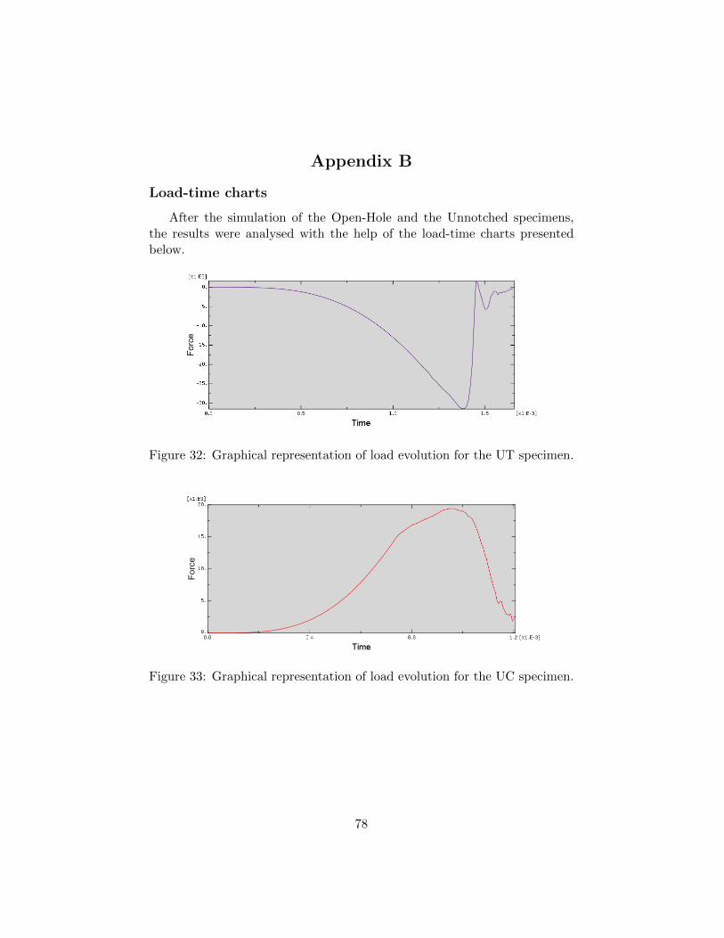
Appendix B
Load-time charts
After the simulation of the Open-Hole and the Unnotched specimens,the results were analysed with the help of the load-time charts presentedbelow.
Figure 32: Graphical representation of load evolution for the UT specimen.
Figure 33: Graphical representation of load evolution for the UC specimen.
78
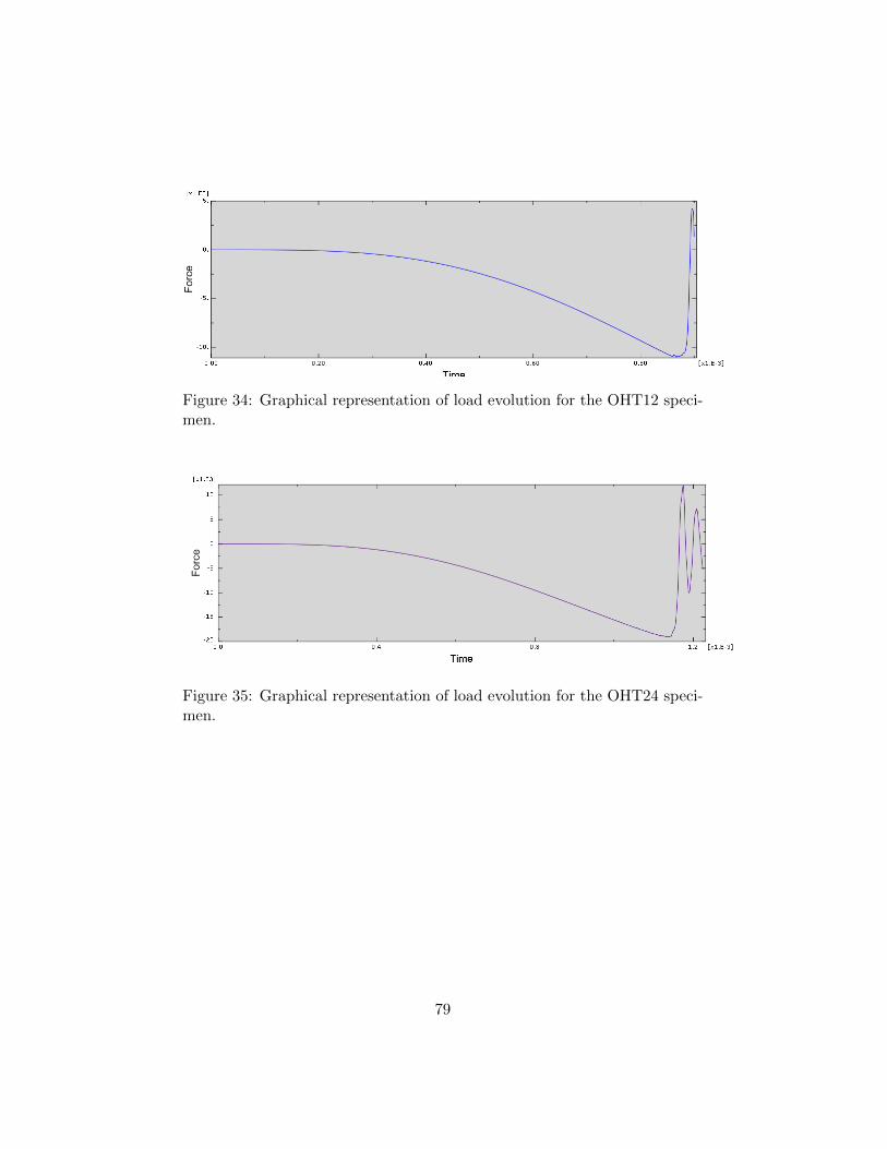
Figure 34: Graphical representation of load evolution for the OHT12 speci-men.
Figure 35: Graphical representation of load evolution for the OHT24 speci-men.
79
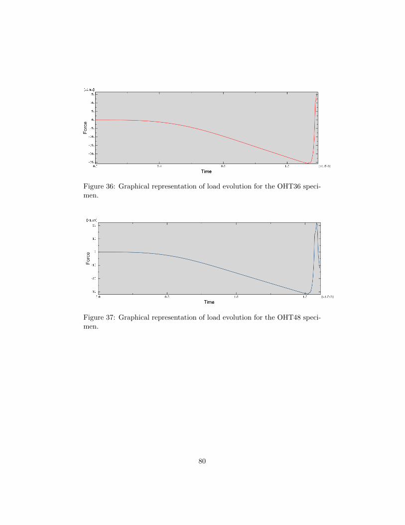
Figure 36: Graphical representation of load evolution for the OHT36 speci-men.
Figure 37: Graphical representation of load evolution for the OHT48 speci-men.
80
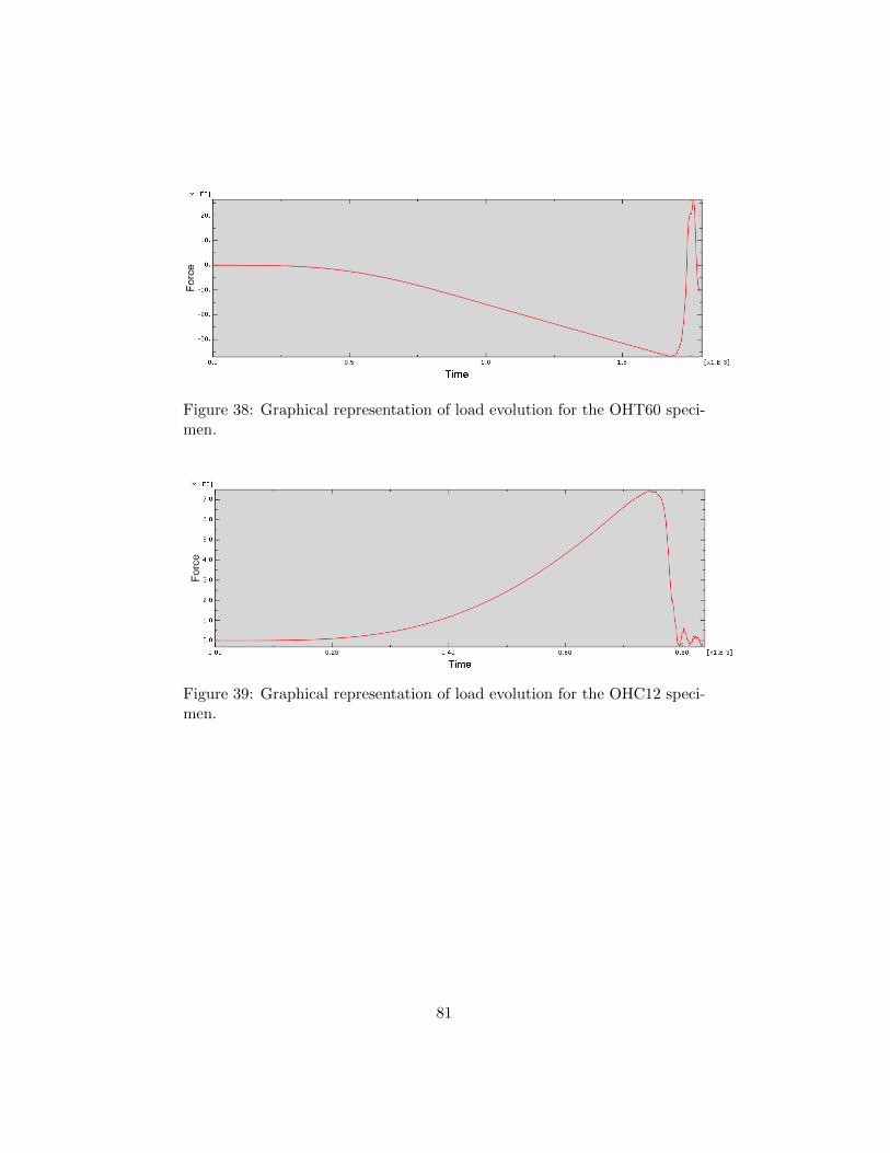
Figure 38: Graphical representation of load evolution for the OHT60 speci-men.
Figure 39: Graphical representation of load evolution for the OHC12 speci-men.
81
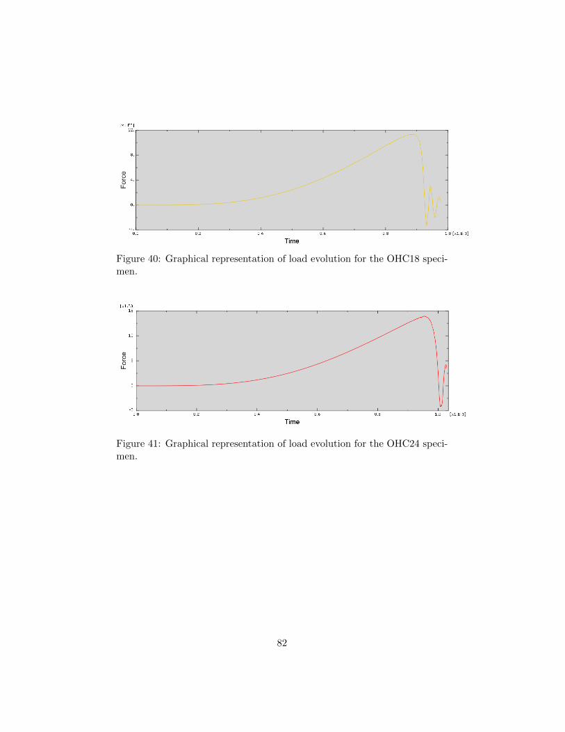
Figure 40: Graphical representation of load evolution for the OHC18 speci-men.
Figure 41: Graphical representation of load evolution for the OHC24 speci-men.
82
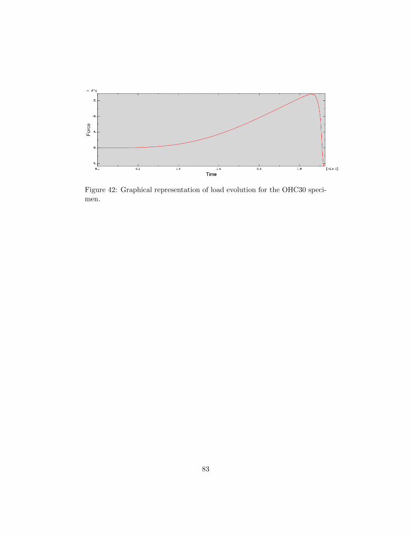
Figure 42: Graphical representation of load evolution for the OHC30 speci-men.
83
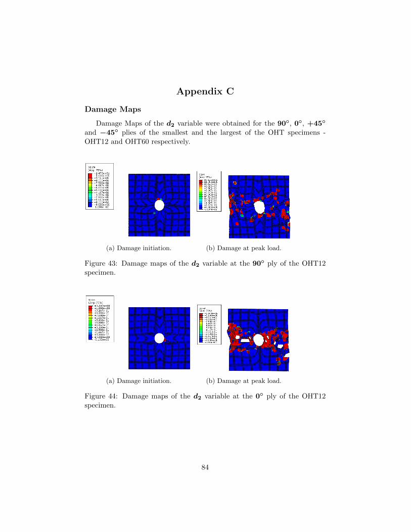
Appendix C
Damage Maps
Damage Maps of the d2 variable were obtained for the 90◦, 0◦, +45◦
and −45◦ plies of the smallest and the largest of the OHT specimens -OHT12 and OHT60 respectively.
(a) Damage initiation. (b) Damage at peak load.
Figure 43: Damage maps of the d2 variable at the 90◦ ply of the OHT12specimen.
(a) Damage initiation. (b) Damage at peak load.
Figure 44: Damage maps of the d2 variable at the 0◦ ply of the OHT12specimen.
84
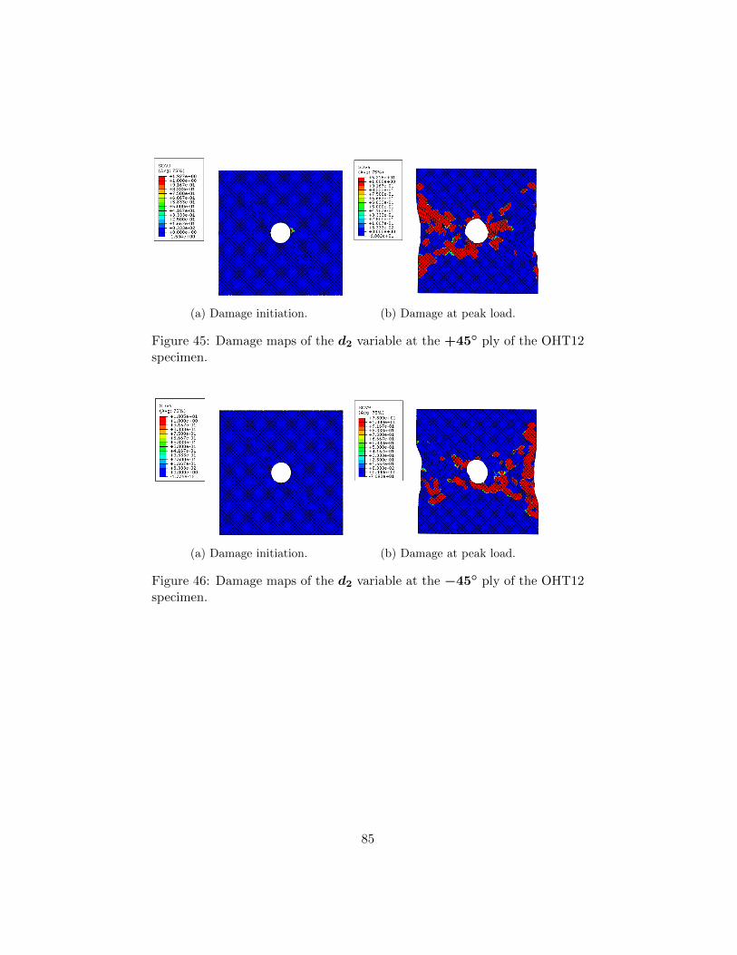
(a) Damage initiation. (b) Damage at peak load.
Figure 45: Damage maps of the d2 variable at the +45◦ ply of the OHT12specimen.
(a) Damage initiation. (b) Damage at peak load.
Figure 46: Damage maps of the d2 variable at the −45◦ ply of the OHT12specimen.
85
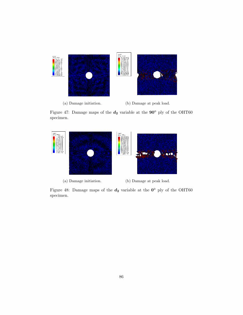
(a) Damage initiation. (b) Damage at peak load.
Figure 47: Damage maps of the d2 variable at the 90◦ ply of the OHT60specimen.
(a) Damage initiation. (b) Damage at peak load.
Figure 48: Damage maps of the d2 variable at the 0◦ ply of the OHT60specimen.
86
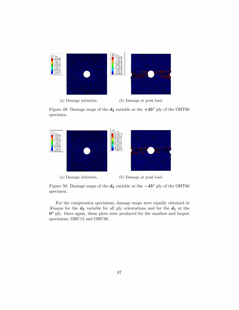
(a) Damage initiation. (b) Damage at peak load.
Figure 49: Damage maps of the d2 variable at the +45◦ ply of the OHT60specimen.
(a) Damage initiation. (b) Damage at peak load.
Figure 50: Damage maps of the d2 variable at the −45◦ ply of the OHT60specimen.
For the compression specimens, damage maps were equally obtained inAbaqus for the d2 variable for all ply orientations and for the d1 at the0◦ ply. Once again, these plots were produced for the smallest and largestspecimens, OHC12 and OHC30.
87
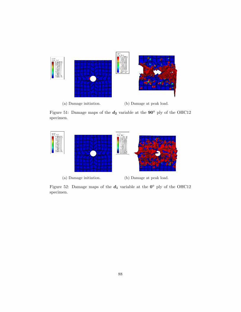
(a) Damage initiation. (b) Damage at peak load.
Figure 51: Damage maps of the d2 variable at the 90◦ ply of the OHC12specimen.
(a) Damage initiation. (b) Damage at peak load.
Figure 52: Damage maps of the d1 variable at the 0◦ ply of the OHC12specimen.
88
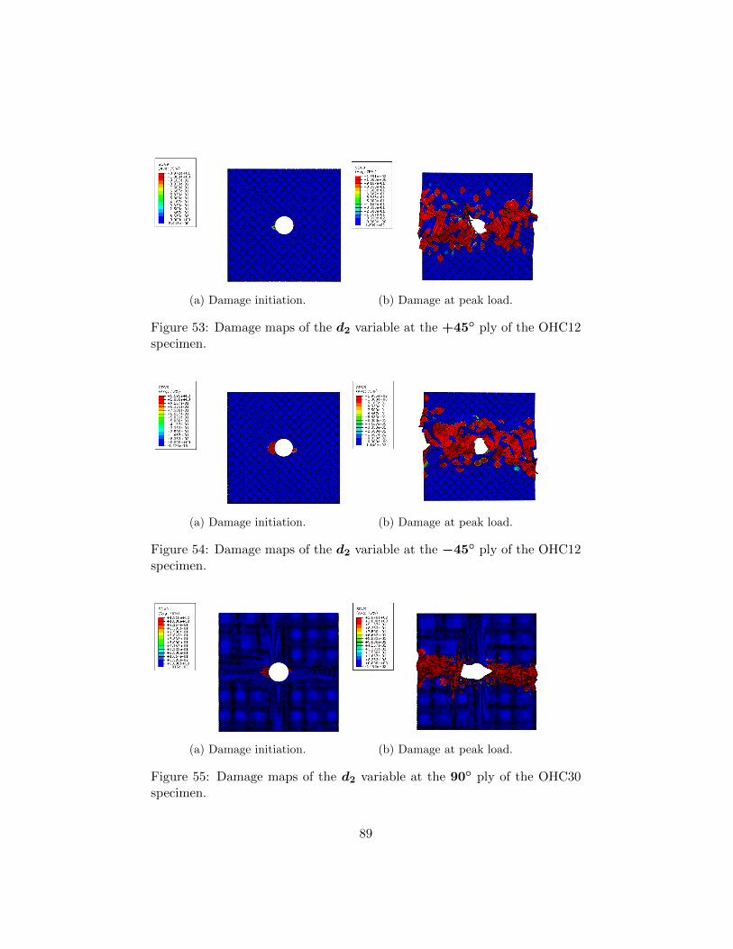
(a) Damage initiation. (b) Damage at peak load.
Figure 53: Damage maps of the d2 variable at the +45◦ ply of the OHC12specimen.
(a) Damage initiation. (b) Damage at peak load.
Figure 54: Damage maps of the d2 variable at the −45◦ ply of the OHC12specimen.
(a) Damage initiation. (b) Damage at peak load.
Figure 55: Damage maps of the d2 variable at the 90◦ ply of the OHC30specimen.
89
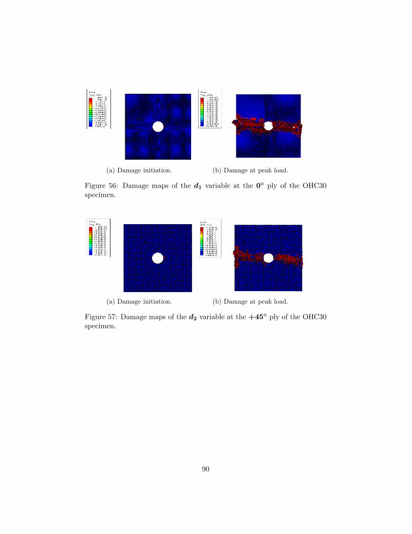
(a) Damage initiation. (b) Damage at peak load.
Figure 56: Damage maps of the d1 variable at the 0◦ ply of the OHC30specimen.
(a) Damage initiation. (b) Damage at peak load.
Figure 57: Damage maps of the d2 variable at the +45◦ ply of the OHC30specimen.
90
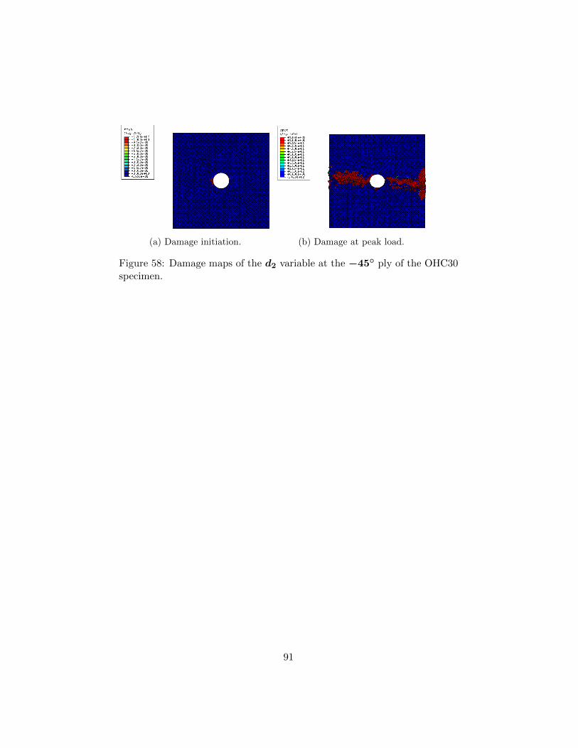
(a) Damage initiation. (b) Damage at peak load.
Figure 58: Damage maps of the d2 variable at the −45◦ ply of the OHC30specimen.
91
References
[1] ESAComp3.5 Commercial software.
[2] American Society for Testing and Materials (ASTM). Stan-dard Test Method for Mode I Interlaminar Fracture Toughness of Uni-directional. Annual Book of ASTM 03 (2004), 1–12.
[3] American Society for Testing and Materials (ASTM). Stan-dard Test Method for In-Plane Shear Response of Polymer Matrix Com-posite Materials by Tensile Test of a 45 Laminate. Annual Book ofASTM 94, Reapproved (2007), 1–7.
[4] American Society for Testing and Materials (ASTM). Stan-dard Test Method for Compressive Properties of Polymer Matrix Com-posite Materials with Unsupported Gage Section by Shear Loading -ASTM D3410, 2008.
[5] American Society for Testing and Materials (ASTM). Stan-dard Test Method for Open-Hole Tensile Strength of Polymer MatrixComposite Laminates - ASTM D5766, 2011.
[6] American Society for Testing and Materials (ASTM). Stan-dard Test Method for Bearing Response of Polymer Matrix CompositeLaminates - ASTM D5961, 2013.
[7] American Society for Testing and Materials (ASTM). Stan-dard Test Method for Open-Hole Compressive Strength of Polymer Ma-trix Composite Laminates - ASTM D6484 / D6484M, 2014.
[8] American Society for Testing and Materials (ASTM). Stan-dard test method for tensile properties of polymer matrix compositematerials - ASTM D3039/D3039M, 2014.
[9] Argon, A. S. Fracture of Composites. In Treatise on Materials Scienceand Technology, A. Press, Ed., 1 ed. New York, 1972.
[10] Aronsson, C., and Backlund, J. Tensile fracture of laminates withcracks. Journal of composite materials, American Society for Compos-ites (1986).
[11] Arteiro, A. Technology development and structural mechanics ofcomposites built of spread tow thin-ply technology. 2012.
92
[12] Bazant, Z., and Oh, B. Crack band theory for fracture of concrete.Materials and Structures (1983).
[13] Benzeggagh, M. L., and Kenane, M. Measurement of mixed-modedelamination fracture toughness of unidirectional glass/epoxy compos-ites with mixed-mode bending apparatus. Composites Science andTechnology 56 (1996), 439–449.
[14] Camanho, P. P., Arteiro, a., Melro, a. R., Catalanotti, G.,and Vogler, M. Three-dimensional invariant-based failure criteria forfibre-reinforced composites. International Journal of Solids and Struc-tures 55 (2014), 92–107.
[15] Camanho, P. P., Bessa, M. A., Catalanotti, G., Vogler, M.,and Rolfes, R. Modeling the inelastic deformation and fracture ofpolymer composites-Part II: Smeared crack model. Mechanics of Ma-terials 59 (2013), 36–49.
[16] Camanho, P. P., and Catalanotti, G. On the relation between themode I fracture toughness of a composite laminate and that of a 0 ply:Analytical model and experimental validation. Engineering FractureMechanics 78, 13 (2011), 2535–2546.
[17] Camanho, P. P., and Lambert, M. A design methodology for me-chanically fastened joints in laminated composite materials. CompositesScience and Technology 66 (2006), 3004–3020.
[18] Camanho, P. P., Maimı, P., and Davila, C. G. Prediction ofsize effects in notched laminates using continuum damage mechanics.Composites Science and Technology 67 (2007), 2715–2727.
[19] Catalanotti, G., Arteiro, A., Hayati, M., and Camanho, P. P.Determination of the mode I crack resistance curve of polymer com-posites using the size-effect law. Engineering Fracture Mechanics 118(2014), 49–65.
[20] Catalanotti, G., Camanho, P. P., and Marques, a. T. Three-dimensional failure criteria for fiber-reinforced laminates. CompositeStructures 95 (2013), 63–79.
[21] Catalanotti, G., Camanho, P. P., Xavier, J., Davila, C. G.,and Marques, a. T. Measurement of resistance curves in the longitu-dinal failure of composites using digital image correlation. CompositesScience and Technology 70, 13 (2010), 1986–1993.
93
[22] Catalanotti, G., Xavier, J., and Camanho, P. P. Measurementof the compressive crack resistance curve of composites using the sizeeffect law. Composites Part A: Applied Science and Manufacturing 56(2014), 300–307.
[23] Davila, C. G., Camanho, P. P., and Rose, C. A. Failure Criteriafor FRP Laminates in Plane Stress.
[24] Davila, C. G., Rose, C. A., and Iarve, E. Modeling Fracture andComplex Crack Networks in Laminated Composites. 2011, pp. 1–56.
[25] D.S. Simulia. Abaqus 6.14 Online Documentation. 2014.
[26] Ercin, G. H. Stress Gradient Effects in Laminated Composites. PhDthesis, 2013.
[27] Jackson, W., and Ratcliffe, J. Measurement of fracture en-ergy for kink-band growth in sandwich specimens. Composites Testingand Model Identification, CompTest2004, University of Bristol, Bristol,UK, Paper no. 24 (2004).
[28] Jirasek, M., and Grassl, P. Evaluation of directional mesh bias inconcrete fracture simulations using continuum damage models. Engi-neering Fracture Mechanics 75 (2008), 1921–1943.
[29] Laffan, M. J., Pinho, S. T., Robinson, P., and Iannucci, L.Measurement of the in situ ply fracture toughness associated with modeI fibre tensile failure in FRP. Part I: Data reduction. Composites Scienceand Technology 70, 4 (2010), 606–613.
[30] Maimı, P., Camanho, P. P., Mayugo, J. A., and Davila, C. G. Acontinuum damage model for composite laminates: Part I - Constitutivemodel. Mechanics of Materials 39 (2007), 897–908.
[31] Maimı, P., Camanho, P. P., Mayugo, J. A., and Davila, C. G.A continuum damage model for composite laminates: Part II - Com-putational implementation and validation. Mechanics of Materials 39(2007), 909–919.
[32] Martin, R. H. ., Elms, T., and Bowron, S. Characterisation ofmode II delamination using the 4 ENF. 4 th European Conference onComposites: Testing and Standardisation (1998), 161–170.
94
[33] Pinho, S. T., Davilla, C. G., Camanho, P. P., Iannucci, L., andRobinson, P. Failure Models and Criteria for FRP Under In-Plane orThree-Dimensional Stress States Including Shear Non-Linearity.
[34] Pinho, S. T., Robinson, P., and Iannucci, L. Fracture tough-ness of the tensile and compressive fibre failure modes in laminatedcomposites. Composites Science and Technology 66 (2006), 2069–2079.
[35] Simulia. Obtaining Improved Results in Abaqus Mixed Mode FractureSimulations Using Cohesive Elements or Surfaces. 2–4.
[36] Song, K., Davila, C. G., and Rose, C. A. Guidelines and param-eter selection for the simulation of progressive delamination. abaqusUser’s Conference, Newport, . . . (2008), 1–15.
[37] Soutis, C., and Fleck, N. Static Compression Failure of CarbonFibre T800/924C Composite Plate with a Single Hole. Journal of Com-posite Materials 24, 5 (1990), 536–558.
[38] Tijssens, M. G. a., Sluys, B. L. J., and Van der Giessen, E.Numerical simulation of quasi-brittle fracture using damaging cohesivesurfaces. European Journal of Mechanics, A/Solids 19 (2000), 761–779.
[39] Turon, A., Camanho, P. P., Costa, J., and Davila, C. G. Adamage model for the simulation of delamination in advanced compos-ites under variable-mode loading. Mechanics of Materials 38 (2006),1072–1089.
[40] Vogler, M., Rolfes, R., and Camanho, P. P. Modeling the inelas-tic deformation and fracture of polymer composites-Part I: Plasticitymodel. Mechanics of Materials 59 (2013), 50–72.
[41] Zhang, C., Binienda, W. K., and Goldberg, R. K. Free-edge ef-fect on the effective stiffness of single-layer triaxially braided composite.Composites Science and Technology 107 (2015), 145–153.
[42] Zhang, J., and Zhang, X. Simulating low-velocity impact induceddelamination in composites by a quasi-static load model with surface-based cohesive contact. Composite Structures 125 (2015), 51–57.
95