Embed Size (px)
Citation preview

VII-1
Part VII: Foundations of Sensor Network Design
Ack: Aman Kansal Copyright © 2005
VII-2
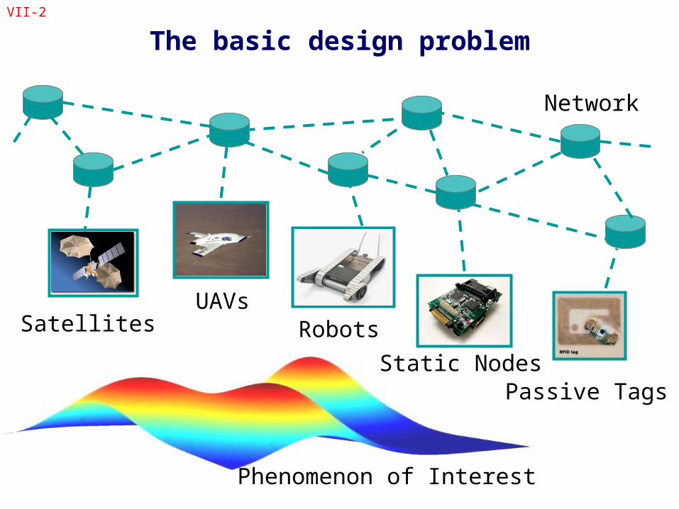
The basic design problem
Phenomenon of Interest
SatellitesUAVs
Robots
Static NodesPassive Tags
Network
VII-3
The basic design problem
• Design a network to extract desired information about a given discrete/continuous phenomenon with high fidelity, low energy and low system cost
• Questions:– Where should the data be collected
– What data and how much data should be collected
– How should the information be communicated
– How should the information be processed
– How can network configuration be adapted in situ
• Single tool does not answer all questions
VII-4
Multiple Tools for Specific Instances
• Problem broken down into smaller parts– Coverage and deployment: Geometric optimization
– Data fusion: Information theory, estimation theory, Bayesian methods
– Communication: network information theory, geometric methods, Bernoulli random graph properties
– Energy performance: Network flow analysis, linear programming
– Configuration adaptation with mobile nodes: adaptive sampling theory, information gain
• Not a comprehensive list

VII-5
Communication
VII-6
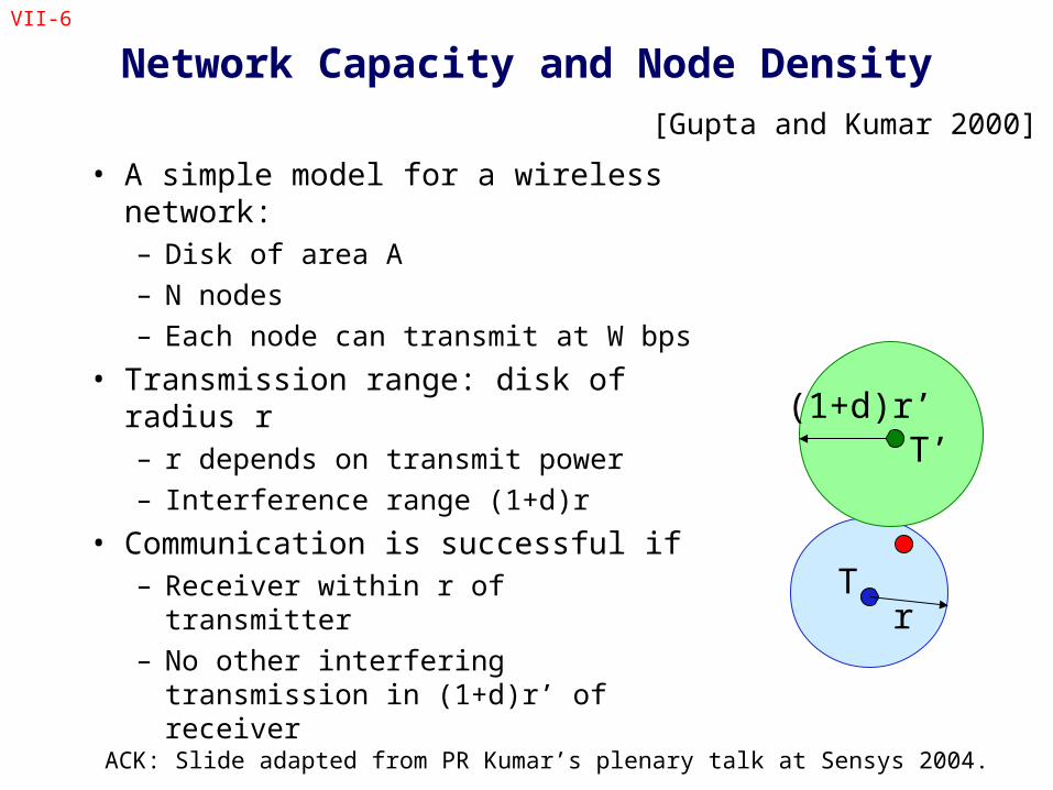
Network Capacity and Node Density
• A simple model for a wireless network:– Disk of area A
– N nodes
– Each node can transmit at W bps
• Transmission range: disk of radius r – r depends on transmit power
– Interference range (1+d)r
• Communication is successful if– Receiver within r of transmitter
– No other interfering transmission in (1+d)r’ of receiver
r
(1+d)r’
T
T’
ACK: Slide adapted from PR Kumar’s plenary talk at Sensys 2004.
[Gupta and Kumar 2000]
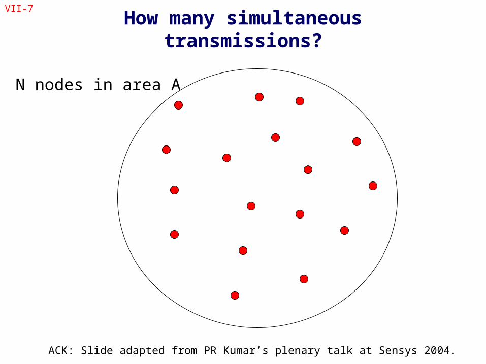
VII-7
How many simultaneous transmissions?
N nodes in area A
ACK: Slide adapted from PR Kumar’s plenary talk at Sensys 2004.
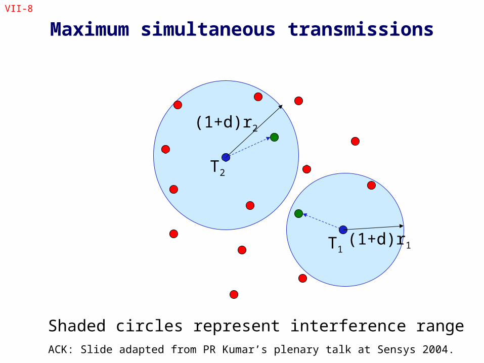
VII-8
Maximum simultaneous transmissions
(1+d)r2
(1+d)r1T1
T2
Shaded circles represent interference rangeACK: Slide adapted from PR Kumar’s plenary talk at Sensys 2004.

VII-9
Maximum simultaneous transmissions
≥ (1+d)r2
T1
T2≥ dr2
≤ r2R2
R1
ACK: Slide adapted from PR Kumar’s plenary talk at Sensys 2004.
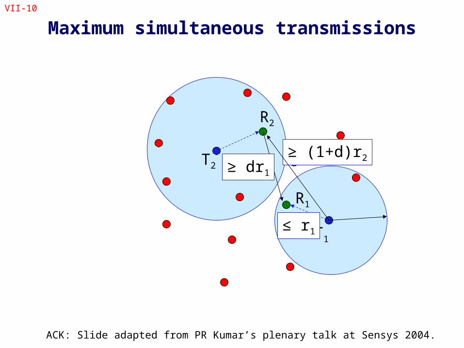
VII-10
Maximum simultaneous transmissions
≥ (1+d)r2
T1
T2 ≥ dr1
≤ r1
R2
R1
ACK: Slide adapted from PR Kumar’s plenary talk at Sensys 2004.
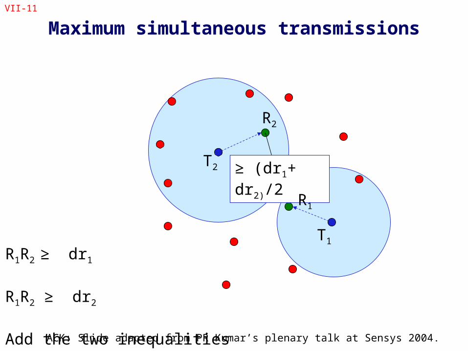
VII-11
Maximum simultaneous transmissions
T1
T2 ≥ (dr1+ dr2)/2
R2
R1
R1R2 ≥ dr1
R1R2 ≥ dr2
Add the two inequalitiesACK: Slide adapted from PR Kumar’s plenary talk at Sensys 2004.
VII-12
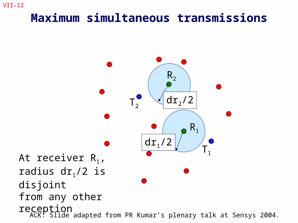
Maximum simultaneous transmissions
T1
T2
dr1/2
R2
R1
At receiver R1, radius dr1/2 is disjoint from any other reception
dr2/2
ACK: Slide adapted from PR Kumar’s plenary talk at Sensys 2004.
VII-13
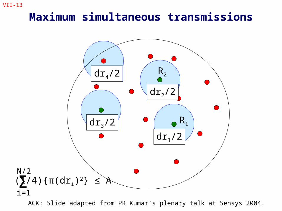
Maximum simultaneous transmissions
dr1/2
R2
R1
dr2/2
dr3/2
dr4/2
Σi=1
N/2(1/4){π(dri)2} ≤ A
ACK: Slide adapted from PR Kumar’s plenary talk at Sensys 2004.
VII-14
Maximum simultaneous transmissions
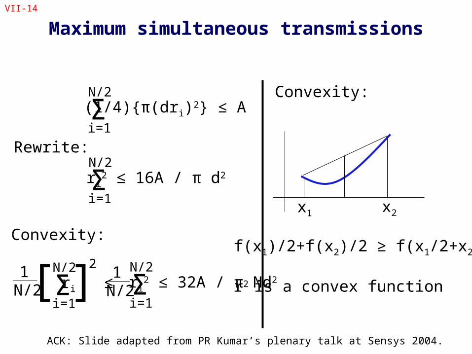
Σi=1
N/2(1/4){π(dri)2} ≤ A
Σi=1
N/2ri
2 ≤ 16A / π d2
Convexity:
x1 x2
f(x1)/2+f(x2)/2 ≥ f(x1/2+x2/2)
r2 is a convex function
Rewrite:
Convexity:
Σi=1
N/2ri
2 ≤ 32A / π Nd2Σi=1
N/2ri ≤
1N/2[ ]
21
N/2
ACK: Slide adapted from PR Kumar’s plenary talk at Sensys 2004.
VII-15
Transport Capacity
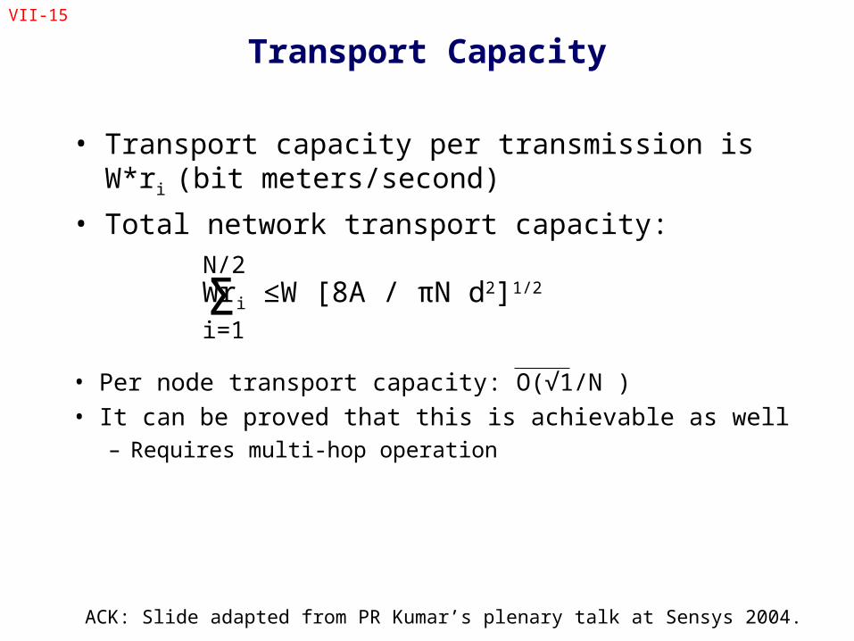
• Transport capacity per transmission is W*ri (bit meters/second)
• Total network transport capacity:
Σi=1
N/2Wri ≤W [8A / πN d2]1/2
• Per node transport capacity: O(√1/N )• It can be proved that this is achievable as well
– Requires multi-hop operation
ACK: Slide adapted from PR Kumar’s plenary talk at Sensys 2004.
VII-16
Design Implications
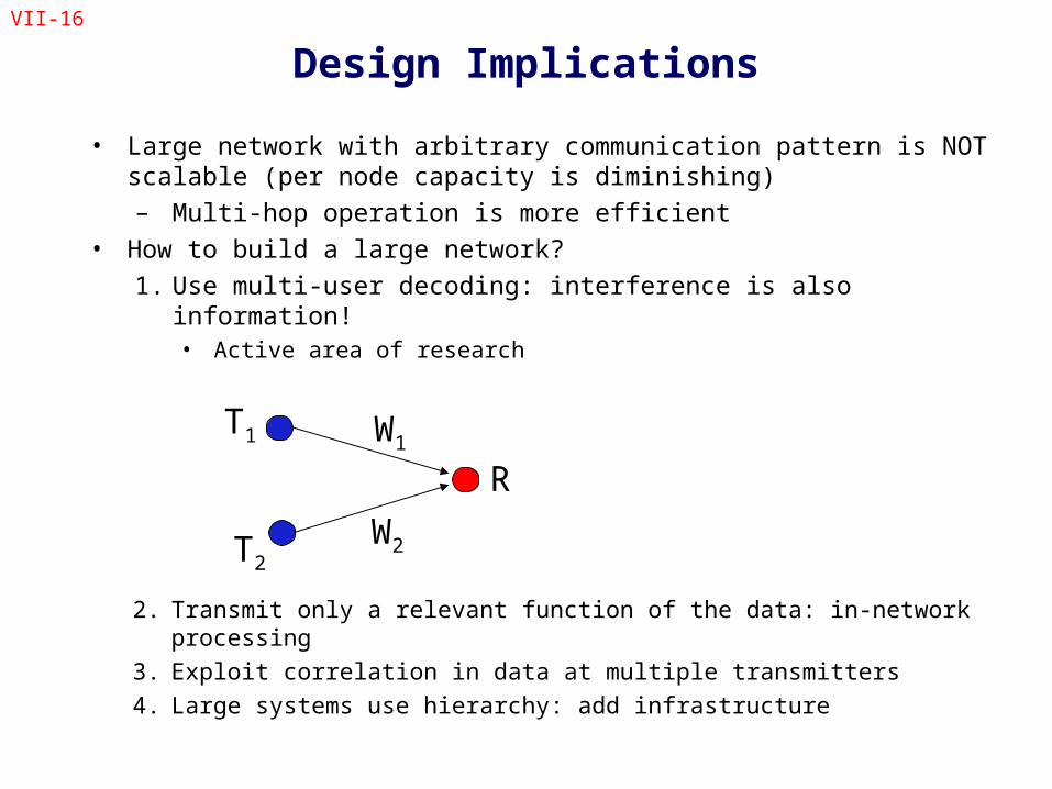
• Large network with arbitrary communication pattern is NOT scalable (per node capacity is diminishing)– Multi-hop operation is more efficient
• How to build a large network?
1. Use multi-user decoding: interference is also information!• Active area of research
W2
W1T1
T2
R
2. Transmit only a relevant function of the data: in-network processing
3. Exploit correlation in data at multiple transmitters
4. Large systems use hierarchy: add infrastructure
VII-17
In Network Processing
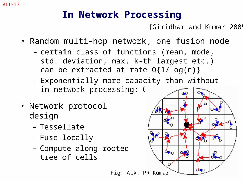
• Random multi-hop network, one fusion node– certain class of functions (mean, mode, std. deviation,
max, k-th largest etc.) can be extracted at rate O{1/log(n)}
– Exponentially more capacity than without in network processing: O(1/n)
• Network protocol design– Tessellate
– Fuse locally
– Compute along rooted tree of cells
Fig. Ack: PR Kumar
[Giridhar and Kumar 2005]
VII-18
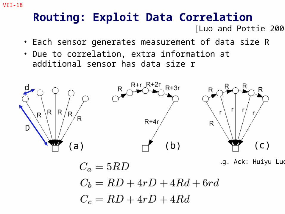
Routing: Exploit Data Correlation
• Each sensor generates measurement of data size R • Due to correlation, extra information at additional sensor
has data size r
Fig. Ack: Huiyu Luo
D
d
(a) (b) (c)
[Luo and Pottie 2005]

VII-19
Data Fusion
VII-20
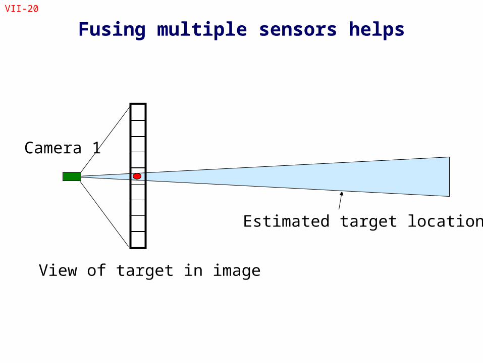
Fusing multiple sensors helps
Camera 1
View of target in image
Estimated target location
VII-21
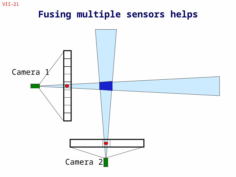
Fusing multiple sensors helps
Camera 2
Camera 1
VII-22
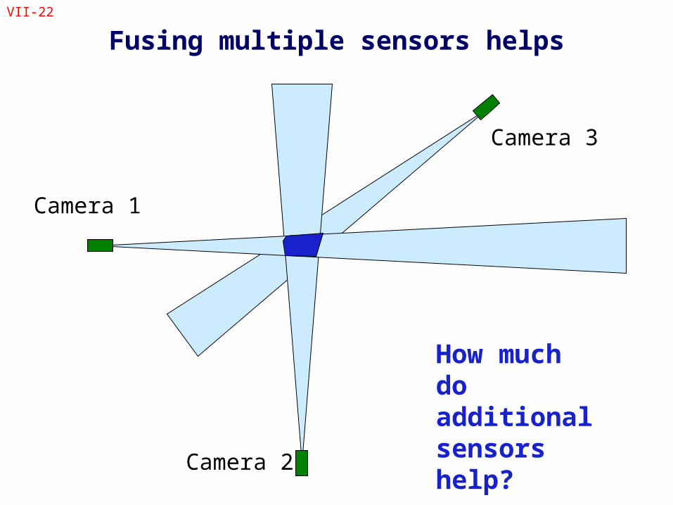
Fusing multiple sensors helps
Camera 1
Camera 2
Camera 3
How much do additional sensors help?
VII-23
Resort to Information Theory
• Model the information content of each sensor• Measure the combined information content of multiple
sensors assuming best possible fusion methods used– Eg. Compute the distortion achieved for a given data size
• Can then determine if the improvement in distortion is worth the extra sensors
VII-24
Measuring Information
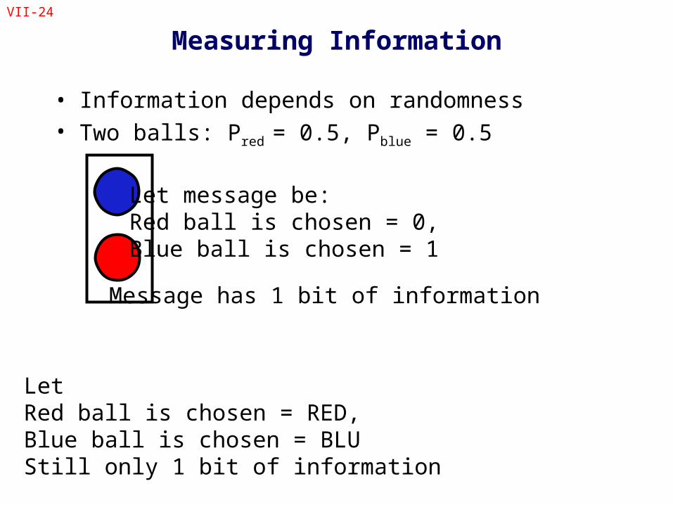
• Information depends on randomness• Two balls: Pred = 0.5, Pblue = 0.5
Message has 1 bit of information
Let message be:Red ball is chosen = 0, Blue ball is chosen = 1
Let Red ball is chosen = RED, Blue ball is chosen = BLUStill only 1 bit of information
VII-25
Measuring Information
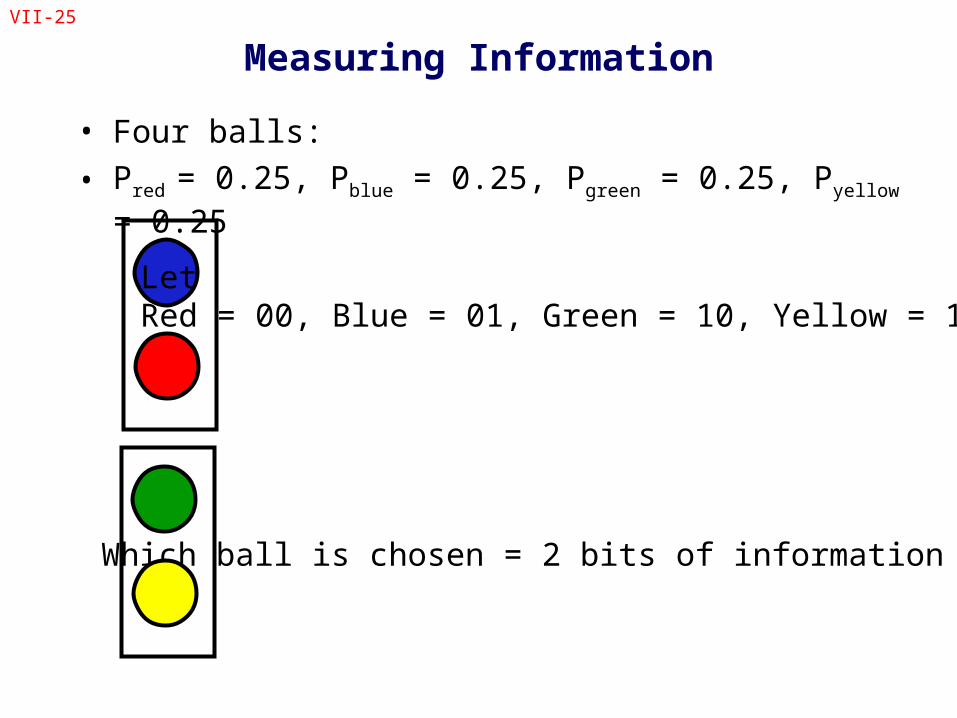
• Four balls:
• Pred = 0.25, Pblue = 0.25, Pgreen = 0.25, Pyellow = 0.25
Which ball is chosen = 2 bits of information
Let Red = 00, Blue = 01, Green = 10, Yellow = 11
VII-26
Measuring Information
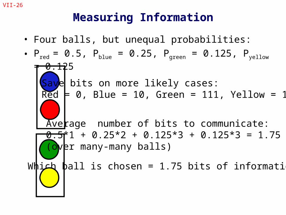
• Four balls, but unequal probabilities:
• Pred = 0.5, Pblue = 0.25, Pgreen = 0.125, Pyellow = 0.125
Which ball is chosen = 1.75 bits of information
Save bits on more likely cases:Red = 0, Blue = 10, Green = 111, Yellow = 110
Average number of bits to communicate:0.5*1 + 0.25*2 + 0.125*3 + 0.125*3 = 1.75(over many-many balls)
VII-27
Measuring Information
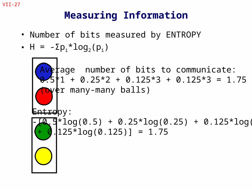
• Number of bits measured by ENTROPY
• H = -Σpi*log2(pi)
Average number of bits to communicate:0.5*1 + 0.25*2 + 0.125*3 + 0.125*3 = 1.75(over many-many balls)
Entropy:-[0.5*log(0.5) + 0.25*log(0.25) + 0.125*log(0.125) + 0.125*log(0.125)] = 1.75
VII-28
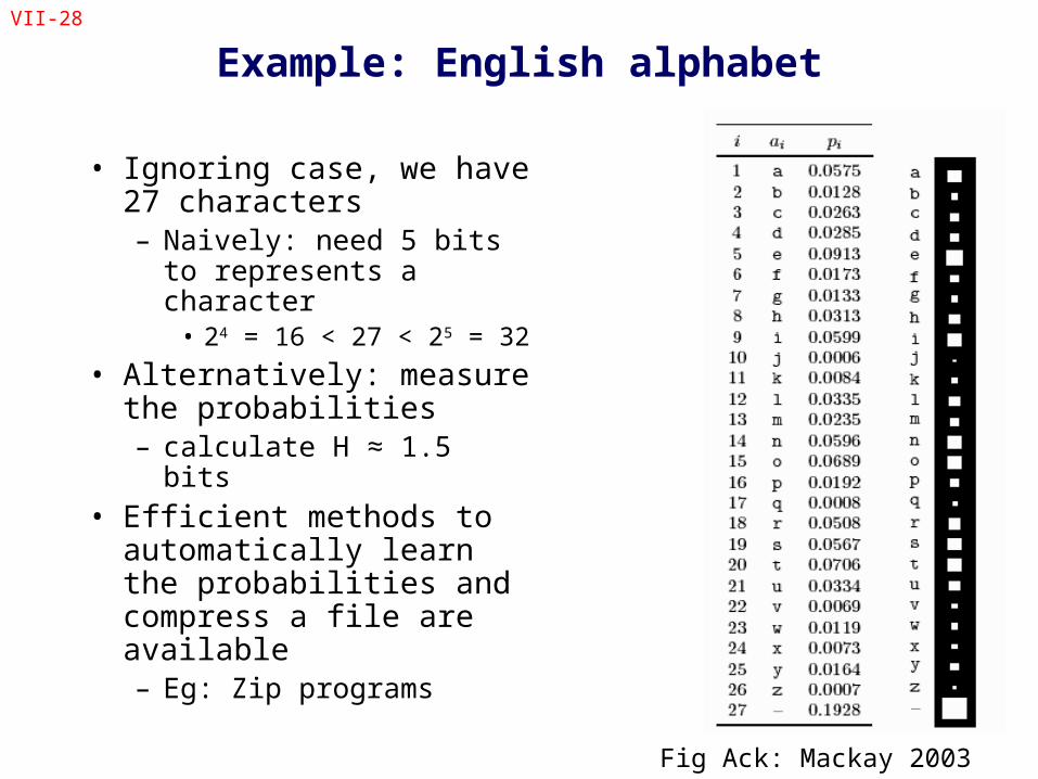
Example: English alphabet
• Ignoring case, we have 27 characters– Naively: need 5 bits to
represents a character• 24 = 16 < 27 < 25 = 32
• Alternatively: measure the probabilities– calculate H ≈ 1.5 bits
• Efficient methods to automatically learn the probabilities and compress a file are available– Eg: Zip programs
Fig Ack: Mackay 2003
VII-29
Conditional Entropy
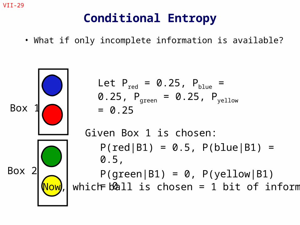
• What if only incomplete information is available?
Let Pred = 0.25, Pblue = 0.25, Pgreen = 0.25, Pyellow = 0.25
Given Box 1 is chosen:
P(red|B1) = 0.5, P(blue|B1) = 0.5,
P(green|B1) = 0, P(yellow|B1) = 0
Box 1
Box 2
Now, which ball is chosen = 1 bit of information
VII-30
Conditional Entropy
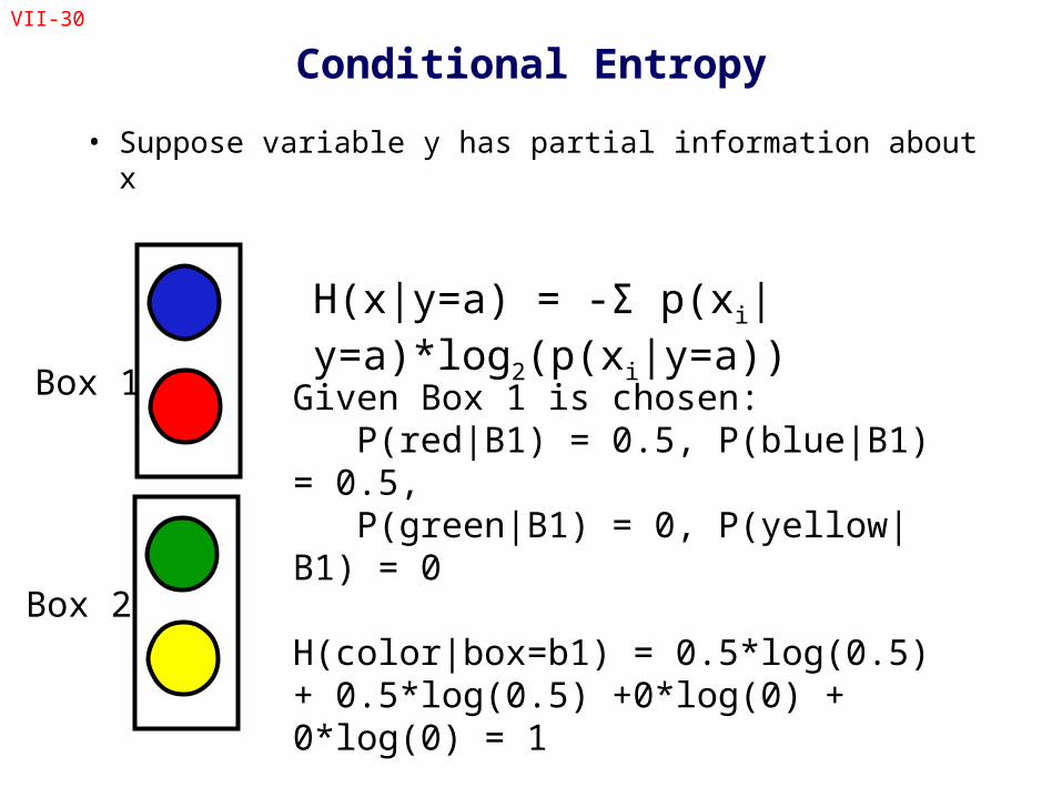
• Suppose variable y has partial information about x
H(x|y=a) = -Σ p(xi|y=a)*log2(p(xi|y=a))
Given Box 1 is chosen: P(red|B1) = 0.5, P(blue|B1) = 0.5, P(green|B1) = 0, P(yellow|B1) = 0
H(color|box=b1) = 0.5*log(0.5) + 0.5*log(0.5) +0*log(0) + 0*log(0) = 1
Box 1
Box 2
VII-31
Conditional Entropy
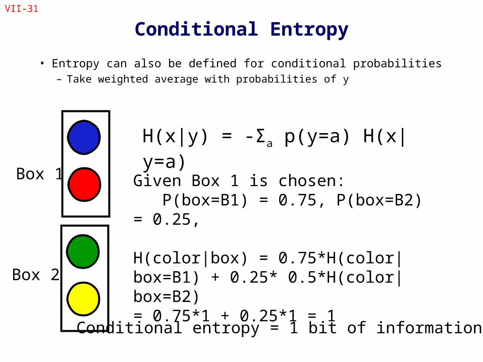
• Entropy can also be defined for conditional probabilities– Take weighted average with probabilities of y
H(x|y) = -Σa p(y=a) H(x|y=a)
Given Box 1 is chosen: P(box=B1) = 0.75, P(box=B2) = 0.25,
H(color|box) = 0.75*H(color|box=B1) + 0.25* 0.5*H(color|box=B2)= 0.75*1 + 0.25*1 = 1
Box 1
Box 2
Conditional entropy = 1 bit of information
VII-32
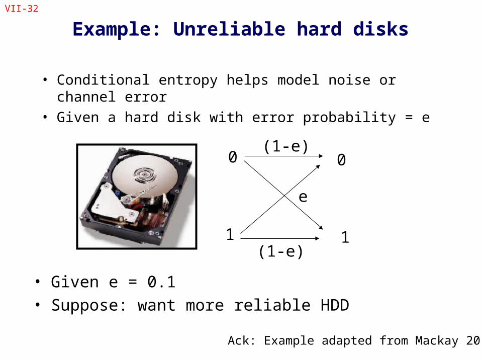
Example: Unreliable hard disks
• Conditional entropy helps model noise or channel error• Given a hard disk with error probability = e
0
1
0
1
(1-e)
e
(1-e)
• Given e = 0.1• Suppose: want more reliable HDD
Ack: Example adapted from Mackay 2003
VII-33
Example: Unreliable hard disks
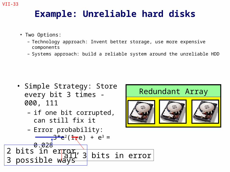
• Two Options: – Technology approach: Invent better storage, use more expensive components– Systems approach: build a reliable system around the unreliable HDD
• Simple Strategy: Store every bit 3 times - 000, 111 – if one bit corrupted, can still
fix it
– Error probability: 3*e2(1-e) + e3 = 0.028
Redundant Array
2 bits in error, 3 possible ways
all 3 bits in error
VII-34
Example: Unreliable hard disks
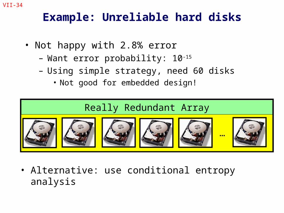
• Not happy with 2.8% error– Want error probability: 10-15
– Using simple strategy, need 60 disks• Not good for embedded design!
• Alternative: use conditional entropy analysis
Really Redundant Array
…
VII-35
Example: Unreliable hard disks
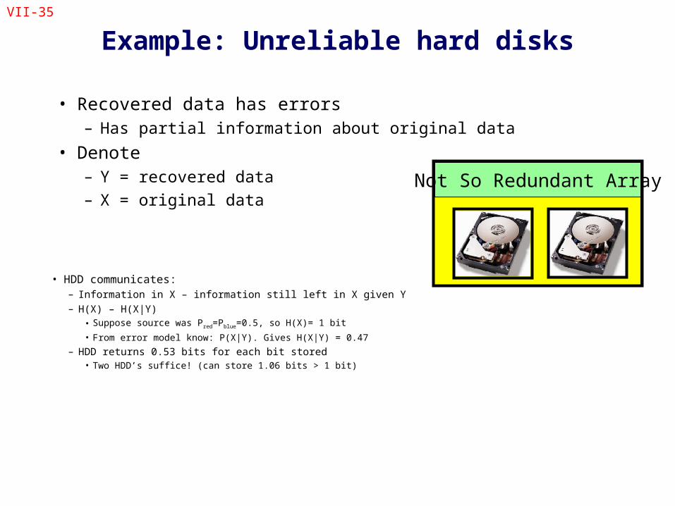
• Recovered data has errors– Has partial information about original data
• Denote– Y = recovered data– X = original data
• HDD communicates:– Information in X – information still left in X given Y– H(X) – H(X|Y)
• Suppose source was Pred=Pblue=0.5, so H(X)= 1 bit
• From error model know: P(X|Y). Gives H(X|Y) = 0.47
– HDD returns 0.53 bits for each bit stored• Two HDD’s suffice! (can store 1.06 bits > 1 bit)
Not So Redundant Array
VII-36
Example: Unreliable hard disks
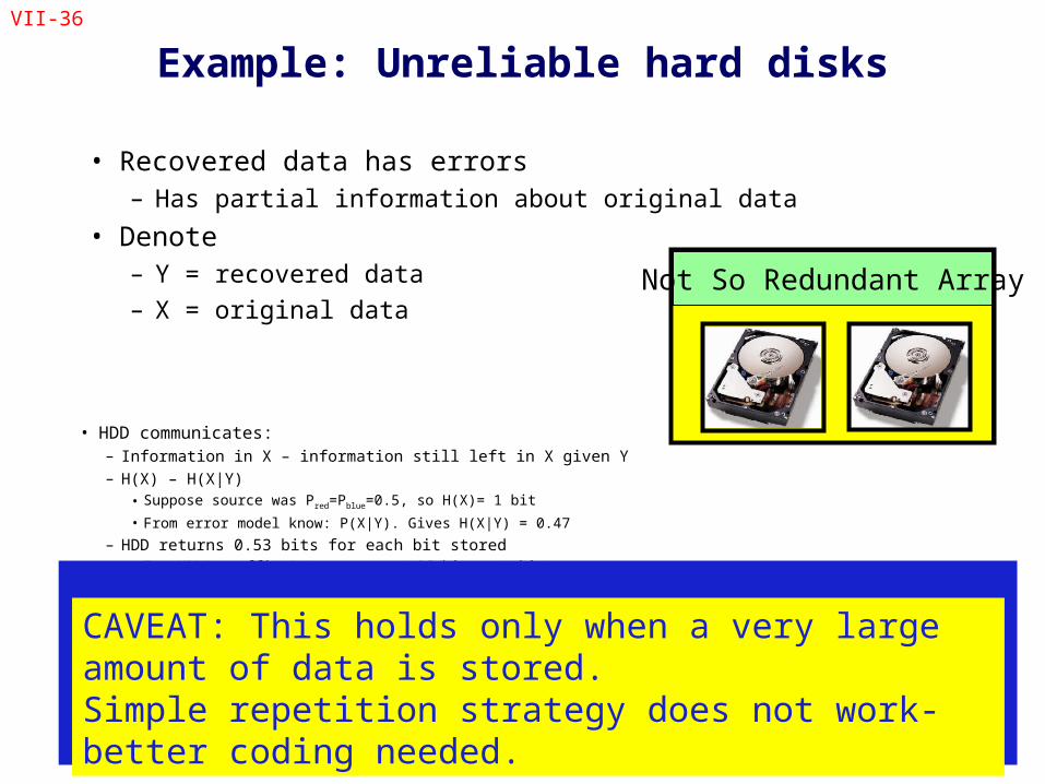
• Recovered data has errors– Has partial information about original data
• Denote– Y = recovered data– X = original data
• HDD communicates:– Information in X – information still left in X given Y– H(X) – H(X|Y)
• Suppose source was Pred=Pblue=0.5, so H(X)= 1 bit
• From error model know: P(X|Y). Gives H(X|Y) = 0.47
– HDD returns 0.53 bits for each bit stored• Two HDD’s suffice! (can store 1.06 bits > 1 bit)
Not So Redundant Array
CAVEAT: This holds only when a very large amount of data is stored. Simple repetition strategy does not work- better coding needed.
VII-37
Mutual Information
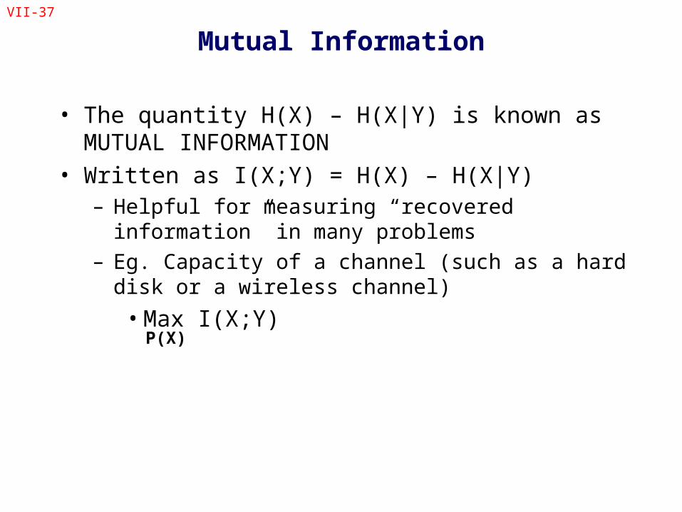
• The quantity H(X) – H(X|Y) is known as MUTUAL INFORMATION
• Written as I(X;Y) = H(X) – H(X|Y)– Helpful for measuring “recovered information” in many
problems
– Eg. Capacity of a channel (such as a hard disk or a wireless channel)
• Max I(X;Y)P(X)
VII-38
Rate Distortion
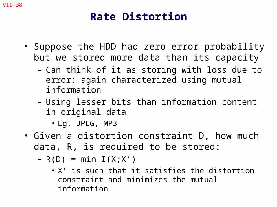
• Suppose the HDD had zero error probability but we stored more data than its capacity– Can think of it as storing with loss due to error: again
characterized using mutual information
– Using lesser bits than information content in original data• Eg. JPEG, MP3
• Given a distortion constraint D, how much data, R, is required to be stored:– R(D) = min I(X;X’)
• X’ is such that it satisfies the distortion constraint and minimizes the mutual information
VII-39
Gaussian Phenomenon
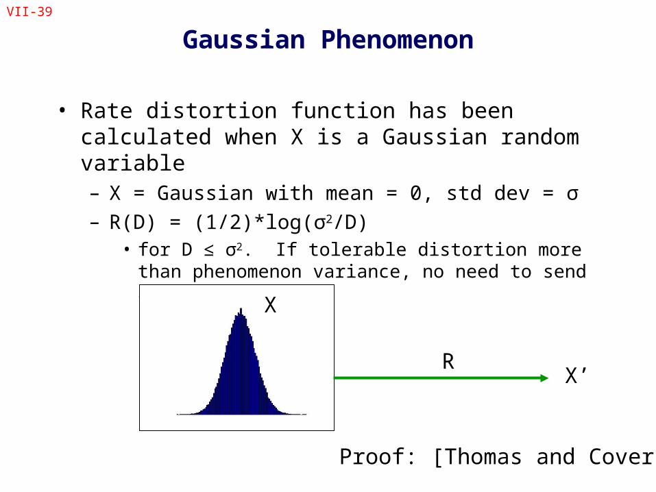
• Rate distortion function has been calculated when X is a Gaussian random variable– X = Gaussian with mean = 0, std dev = σ– R(D) = (1/2)*log(σ2/D)
• for D ≤ σ2. If tolerable distortion more than phenomenon variance, no need to send any data
X
X’R
Proof: [Thomas and Cover]
VII-40
Effect of Sensing Noise
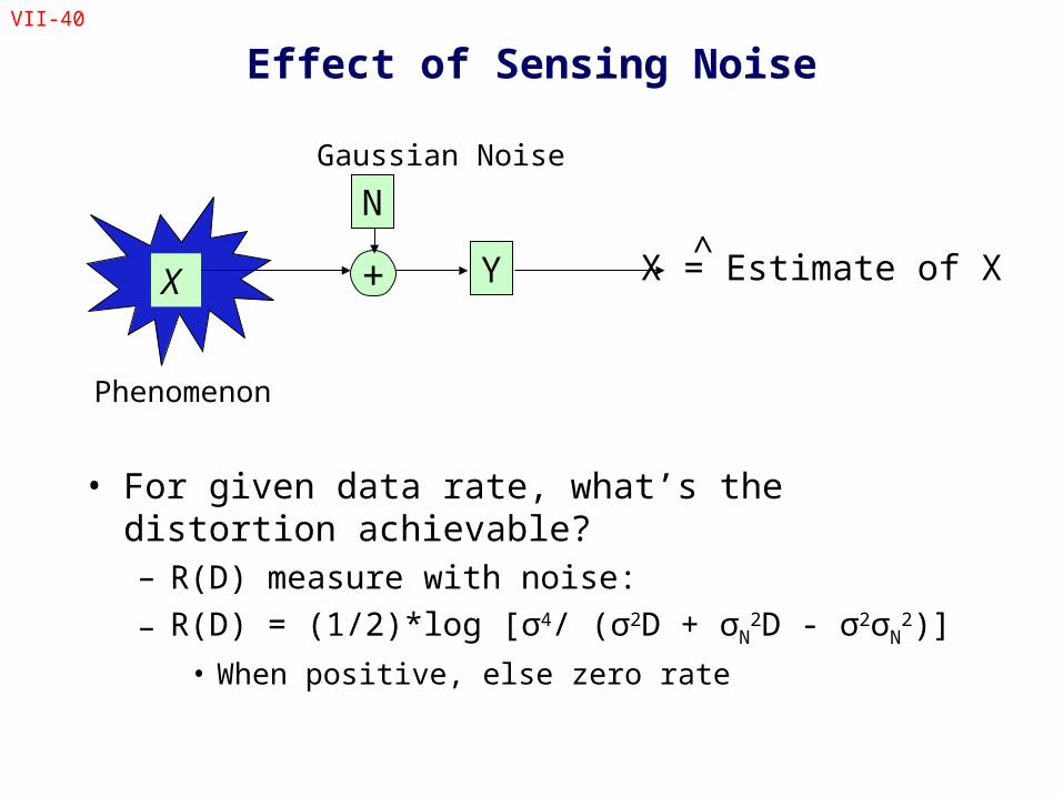
• For given data rate, what’s the distortion achievable?– R(D) measure with noise:
– R(D) = (1/2)*log [σ4/ (σ2D + σN2D - σ2σN
2)]
• When positive, else zero rate
X
Phenomenon
+
N
Y X = Estimate of X^
Gaussian Noise
VII-41
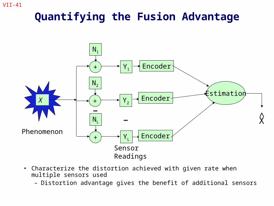
Quantifying the Fusion Advantage
• Characterize the distortion achieved with given rate when multiple sensors used– Distortion advantage gives the benefit of additional sensors
Phenomenon
+
N1
Y1
+
NL
YL
Estimation
Sensor Readings
+
N2
Y2
…X
X̂…
Encoder
Encoder
Encoder
VII-42
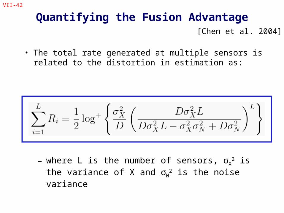
Quantifying the Fusion Advantage
• The total rate generated at multiple sensors is related to the distortion in estimation as:
[Chen et al. 2004]
– where L is the number of sensors, σX2 is the variance of X
and σN2 is the noise variance
VII-43
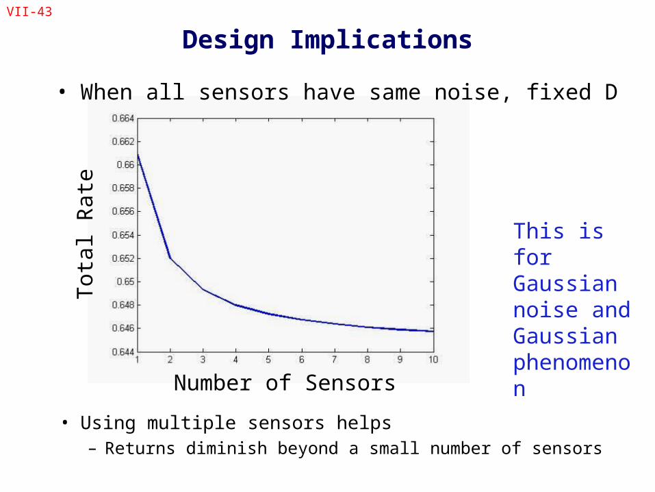
Design Implications
• When all sensors have same noise, fixed D
• Using multiple sensors helps– Returns diminish beyond a small number of sensors
Number of Sensors
Tot
al
Rat
e This is for Gaussian noise and Gaussian phenomenon
VII-44
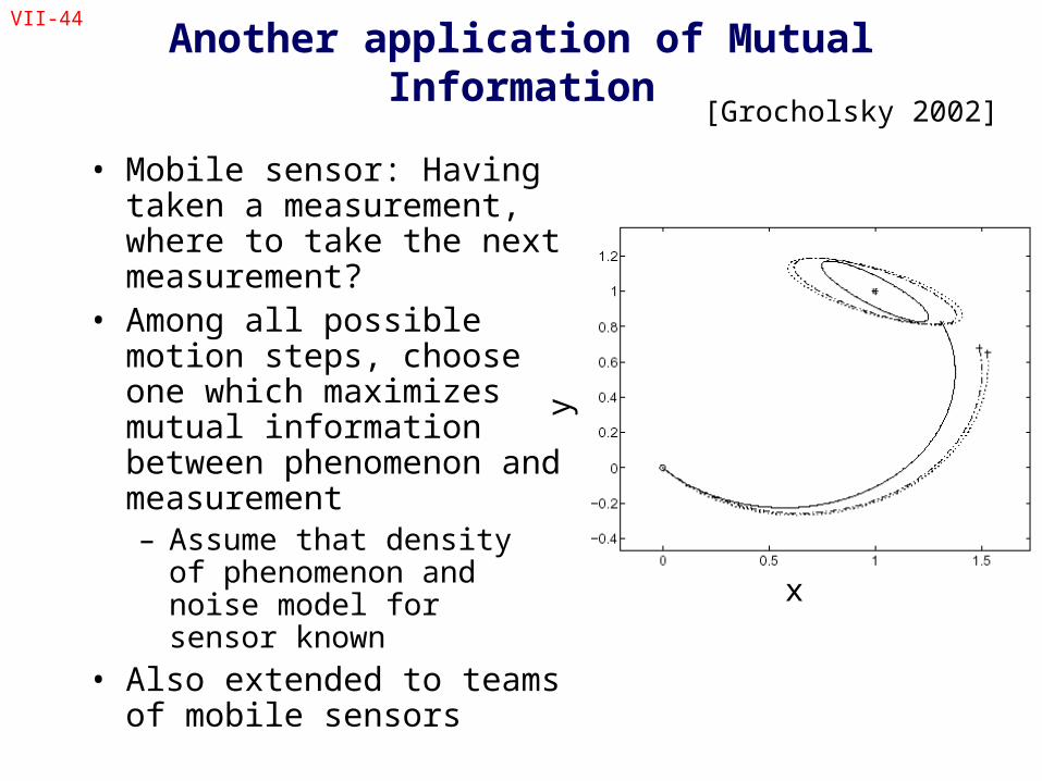
Another application of Mutual Information
• Mobile sensor: Having taken a measurement, where to take the next measurement?
• Among all possible motion steps, choose one which maximizes mutual information between phenomenon and measurement– Assume that density of
phenomenon and noise model for sensor known
• Also extended to teams of mobile sensors
[Grocholsky 2002]
xy

VII-45
Coverage and Deployment
VII-46
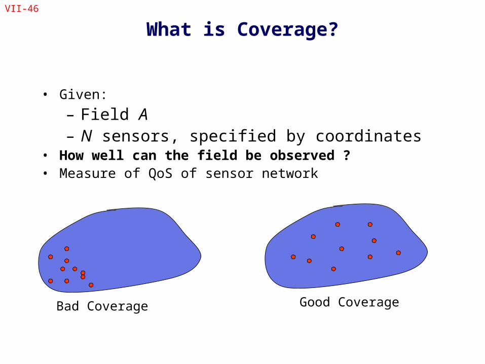
What is Coverage?
• Given:
– Field A– N sensors, specified by coordinates
• How well can the field be observed ?• Measure of QoS of sensor network
Bad Coverage Good Coverage
VII-47
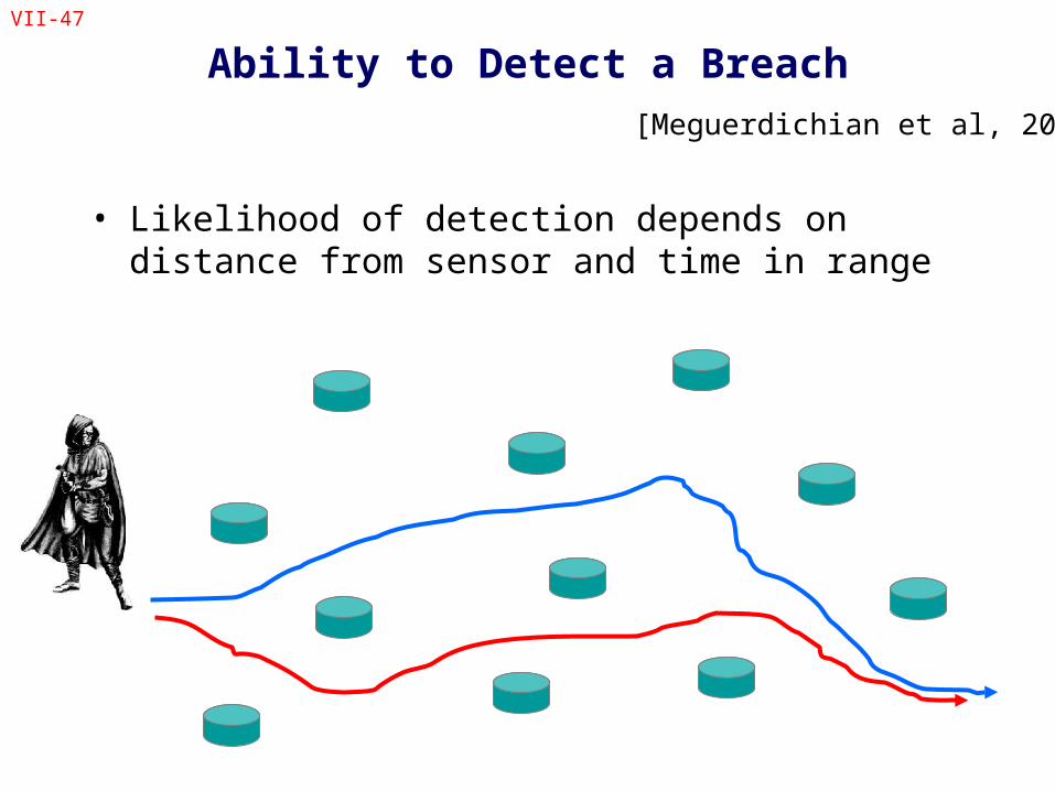
Ability to Detect a Breach
• Likelihood of detection depends on distance from sensor and time in range
[Meguerdichian et al, 2001]
VII-48
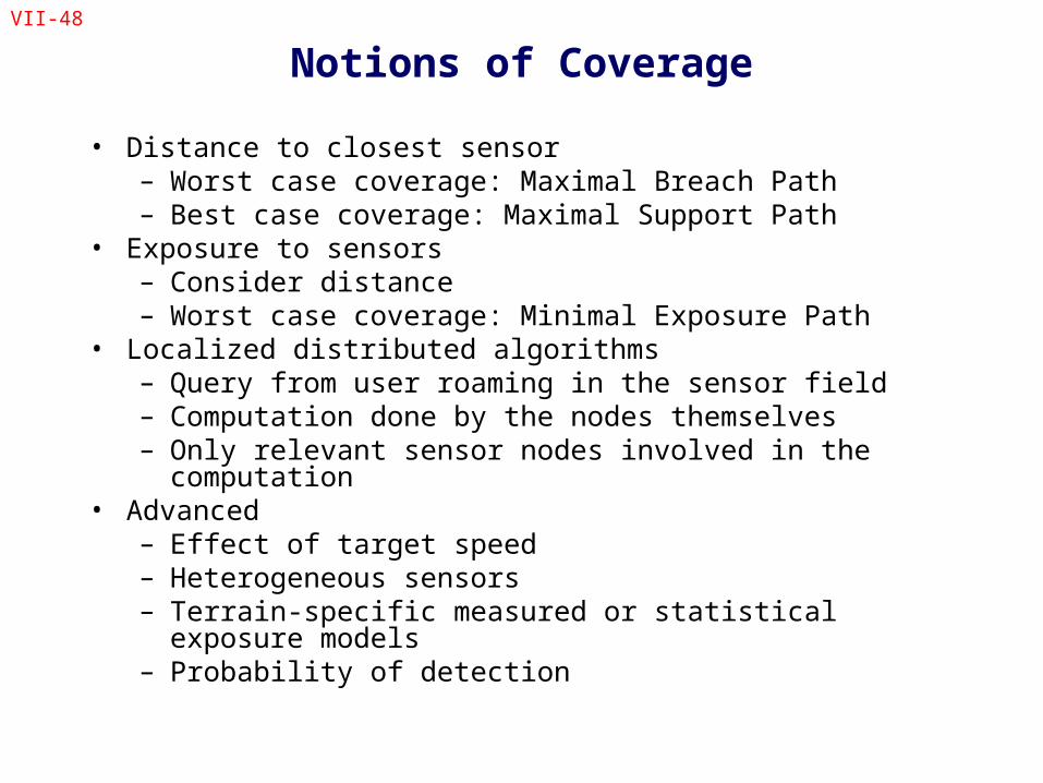
Notions of Coverage
• Distance to closest sensor– Worst case coverage: Maximal Breach Path– Best case coverage: Maximal Support Path
• Exposure to sensors– Consider distance– Worst case coverage: Minimal Exposure Path
• Localized distributed algorithms– Query from user roaming in the sensor field– Computation done by the nodes themselves– Only relevant sensor nodes involved in the computation
• Advanced– Effect of target speed– Heterogeneous sensors– Terrain-specific measured or statistical exposure models– Probability of detection
VII-49
Problem Formulation
• Given:– Initial location (I) of an agent– Final location (F) of an agent
• Find:– Maximal Breach Path:
• Path along which the probability of detection is minimum
• Represents worst case coverage
– Maximal Support Path:• Path along which the probability of detection is maximum
• Represents best case coverage
VII-50
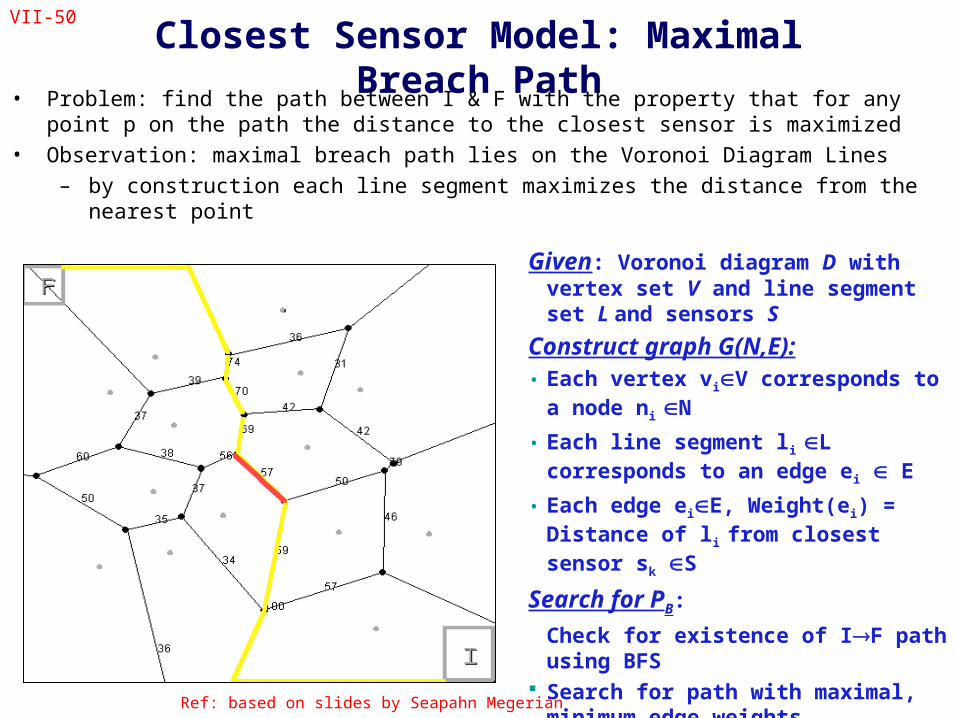
Closest Sensor Model: Maximal Breach Path• Problem: find the path between I & F with the property that for any point p on the path the
distance to the closest sensor is maximized• Observation: maximal breach path lies on the Voronoi Diagram Lines
– by construction each line segment maximizes the distance from the nearest point
Given: Voronoi diagram D with vertex set V and line segment set L and sensors S
Construct graph G(N,E): • Each vertex viV corresponds to a
node ni N
• Each line segment li L corresponds to an edge ei E
• Each edge eiE, Weight(ei) = Distance of li from closest sensor sk S
Search for PB:
Check for existence of IF path using BFS
Search for path with maximal, minimum edge weights
Ref: based on slides by Seapahn Megerian
VII-51
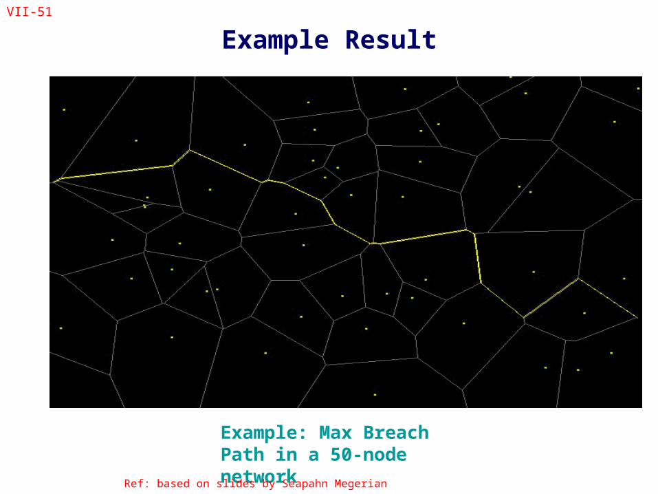
Example Result
Example: Max Breach Path in a 50-node network
Ref: based on slides by Seapahn Megerian
VII-52
Maximal Support
• Given: Field A instrumented with sensors; areas I and F.
• Problem: Identify PS, the maximal support path in S, starting in I and ending in F.
• PS is defined as a path with the property that for any point p on the path PS , the distance from p to the closest sensor is minimized.
VII-53
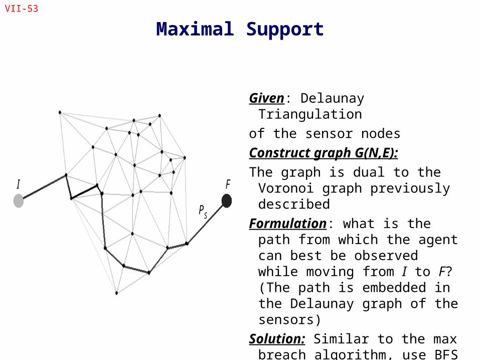
Maximal Support
Given: Delaunay Triangulation
of the sensor nodes
Construct graph G(N,E):
The graph is dual to the Voronoi graph previously described
Formulation: what is the path from which the agent can best be observed while moving from I to F? (The path is embedded in the Delaunay graph of the sensors)
Solution: Similar to the max breach algorithm, use BFS and Binary Search to find the shortest path on the Delaunay graph.
I F
PS
VII-54
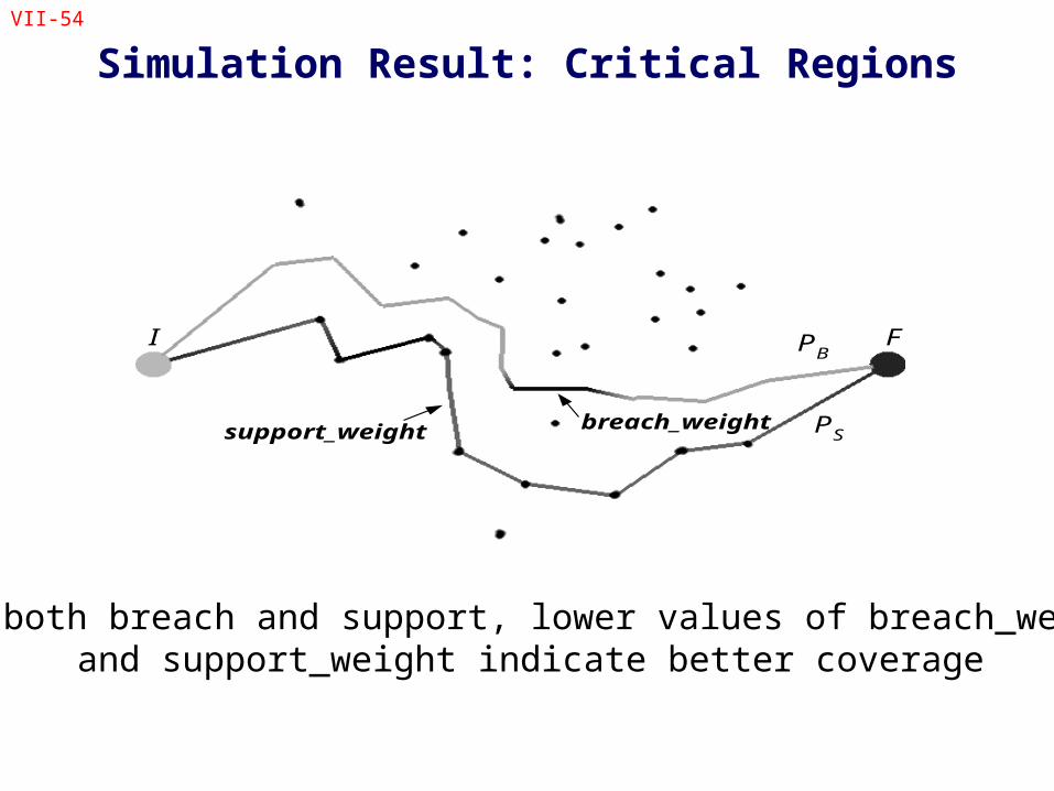
Simulation Result: Critical Regions
I FPB
PSsupport_weight breach_weight
For both breach and support, lower values of breach_weightand support_weight indicate better coverage
VII-55
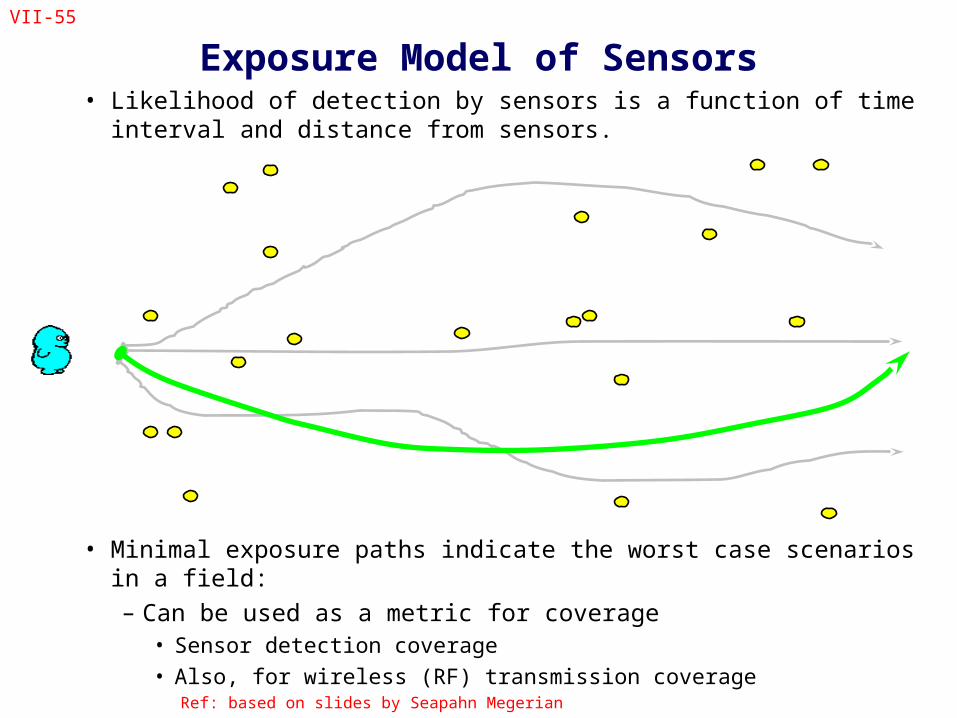
Exposure Model of Sensors• Likelihood of detection by sensors is a function of time interval and
distance from sensors.
• Minimal exposure paths indicate the worst case scenarios in a field:– Can be used as a metric for coverage
• Sensor detection coverage
• Also, for wireless (RF) transmission coverageRef: based on slides by Seapahn Megerian
VII-56
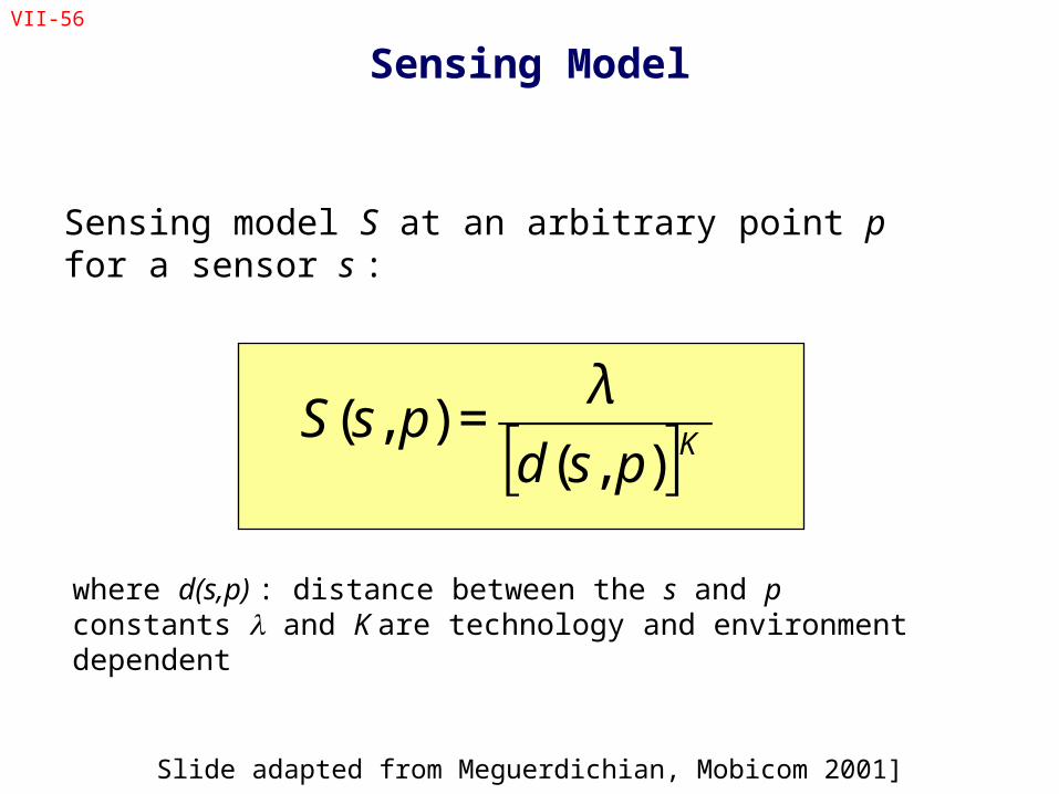
Sensing Model
[ ]KpsdpsS
),(),(
λ=
Sensing model S at an arbitrary point p for a sensor s :
where d(s,p) : distance between the s and p constants and K are technology and environment dependent
Slide adapted from Meguerdichian, Mobicom 2001]
VII-57
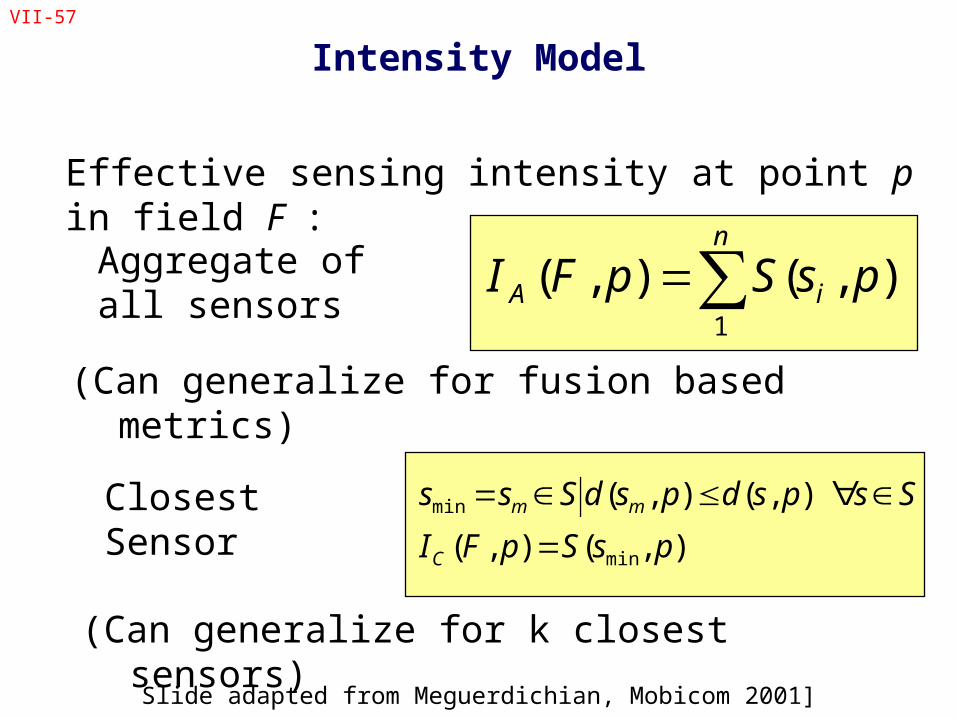
Effective sensing intensity at point p in field F :
∑=n
iA psSpFI1
),(),(
),(),(
),(),(
min
min
psSpFI
SspsdpsdSss
C
mm
=
∈∀≤∈=
Aggregate of all sensors
Closest Sensor
(Can generalize for k closest sensors)
Slide adapted from Meguerdichian, Mobicom 2001]
(Can generalize for fusion based metrics)
Intensity Model
VII-58
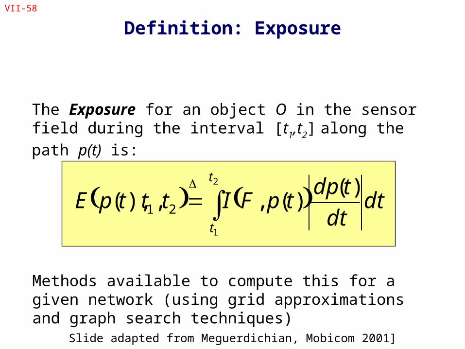
Definition: Exposure
The Exposure for an object O in the sensor field during the interval [t1,t2] along the path p(t) is:
( ) ( )∫Δ
=2
1
)()(, ,),( 21
t
t
dtdt
tdptpFItttpE
Methods available to compute this for a given network (using grid approximations and graph search techniques)
Slide adapted from Meguerdichian, Mobicom 2001]
VII-59
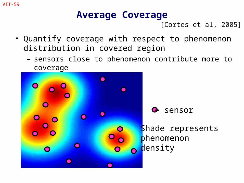
Average Coverage
• Quantify coverage with respect to phenomenon distribution in covered region– sensors close to phenomenon contribute more to coverage
[Cortes et al, 2005]
Shade represents phenomenon density
= sensor
VII-60
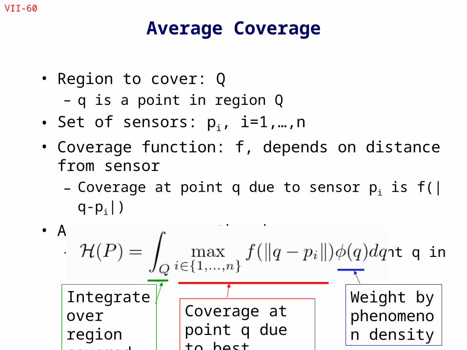
Average Coverage
• Region to cover: Q – q is a point in region Q
• Set of sensors: pi, i=1,…,n
• Coverage function: f, depends on distance from sensor – Coverage at point q due to sensor pi is f(|q-pi|)
• Average coverage then becomes– Considering best sensor for each point q in Q
Coverage at point q due to best sensor
Weight by phenomenon density
Integrate over region covered
VII-61
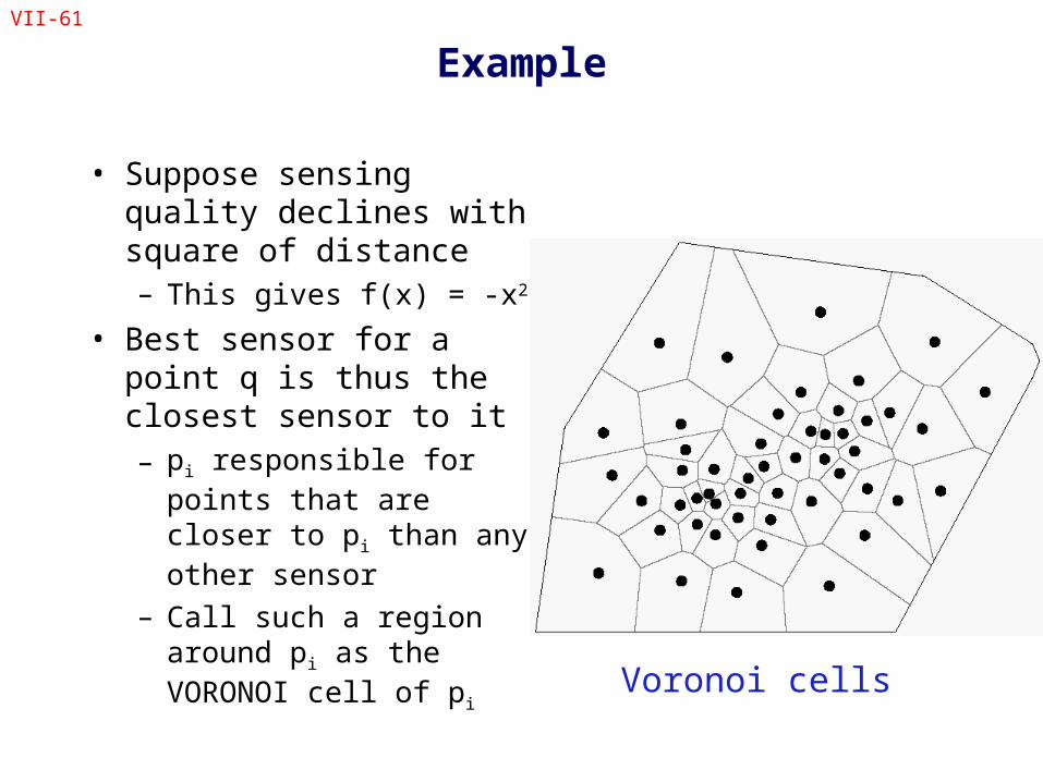
Example
• Suppose sensing quality declines with square of distance– This gives f(x) = -x2
• Best sensor for a point q is thus the closest sensor to it– pi responsible for points
that are closer to pi than any other sensor
– Call such a region around pi as the VORONOI cell of pi
Voronoi cells
VII-62
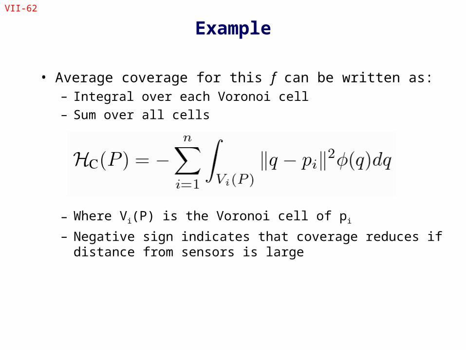
Example
• Average coverage for this f can be written as:– Integral over each Voronoi cell
– Sum over all cells
– Where Vi(P) is the Voronoi cell of pi
– Negative sign indicates that coverage reduces if distance from sensors is large
VII-63
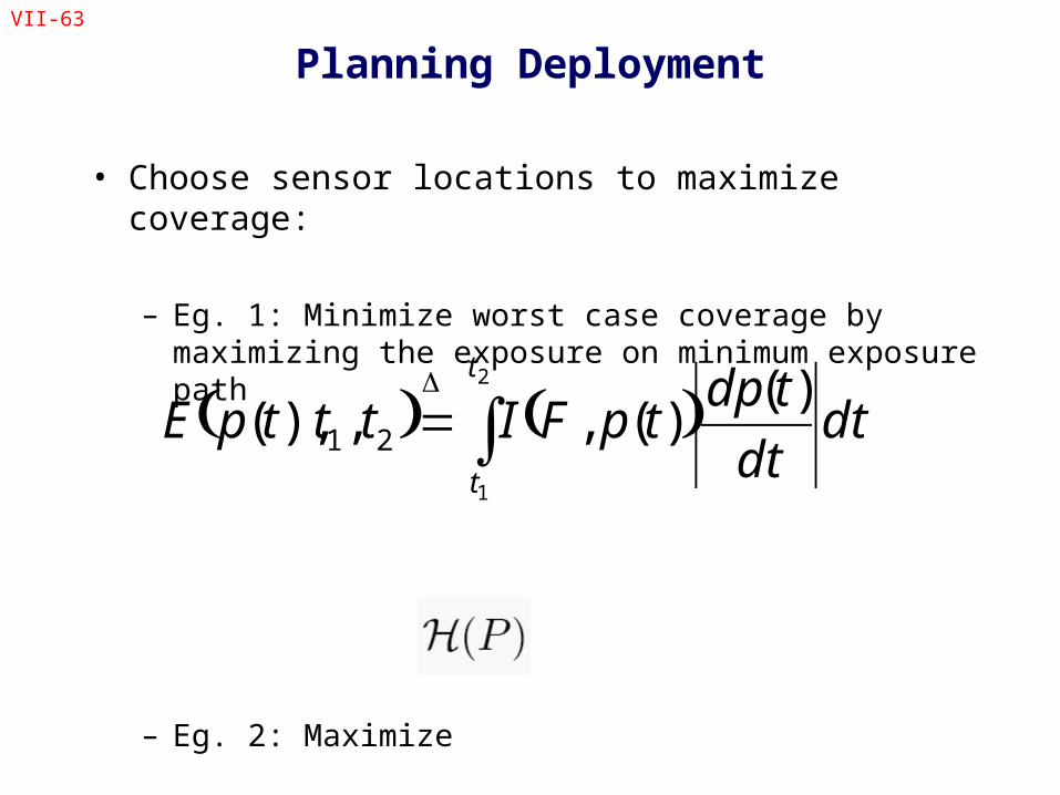
Planning Deployment
• Choose sensor locations to maximize coverage:
– Eg. 1: Minimize worst case coverage by maximizing the exposure on minimum exposure path
– Eg. 2: Maximize
( ) ( )∫Δ
=2
1
)()(, ,),( 21
t
t
dtdt
tdptpFItttpE
VII-64
Adapting Deployment at Real Time
• Suppose nodes are mobile• Need distributed algorithm that allows nodes to change
their locations in order to maximize coverage– Algorithm should use only local information and not the
global view of the network
• One method to compute optima: gradient descent
VII-65
Gradient Descent
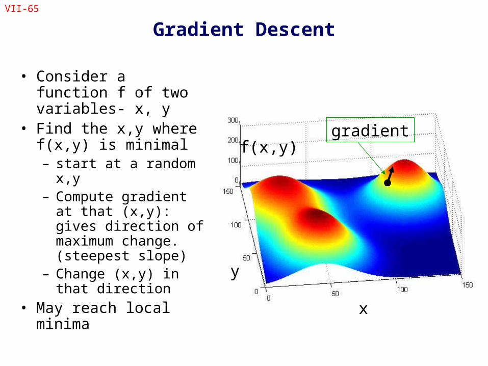
• Consider a function f of two variables- x, y
• Find the x,y where f(x,y) is minimal– start at a random x,y– Compute gradient at
that (x,y): gives direction of maximum change. (steepest slope)
– Change (x,y) in that direction
• May reach local minima x
y
f(x,y)gradient
VII-66
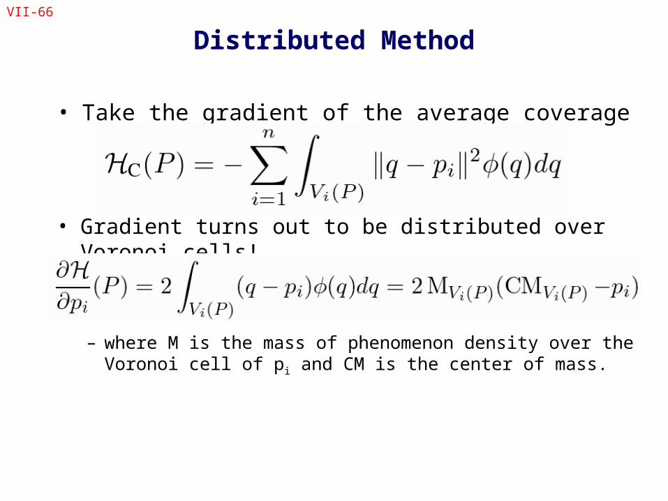
Distributed Method
• Take the gradient of the average coverage
• Gradient turns out to be distributed over Voronoi cells!
– where M is the mass of phenomenon density over the Voronoi cell of pi and CM is the center of mass.
VII-67
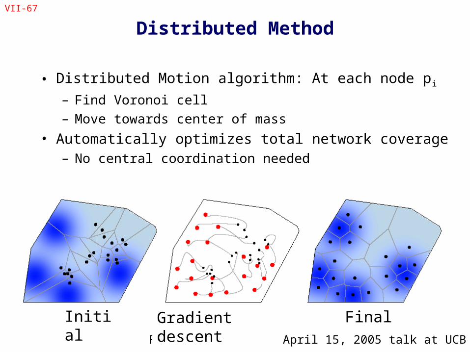
Distributed Method
• Distributed Motion algorithm: At each node pi
– Find Voronoi cell
– Move towards center of mass
• Automatically optimizes total network coverage – No central coordination needed
Fig. Ack: F Bullo, April 15, 2005 talk at UCB
Initial Gradient descent Final
VII-68
Parting Thoughts on Coverage
• Fundamental question: Given an area A and the desired coverage– What is the minimum number of nodes required to achieve the
desired coverage given the deployment scheme ?– What is the probability of achieving the desired coverage for a
random deployment ?
• Things to ponder about– What is a good measure of coverage?– What is the mapping from probability of detection to coverage ?– Sophisticated sensing model
• Directional Sensing
• Effect of obstacles
• More than one type of sensors
• Speed dependence
– Deploying nodes to achieve coverage

VII-69
Energy Performance
VII-70
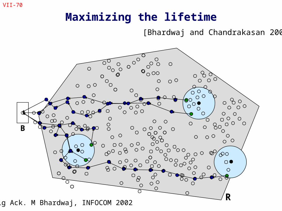
Maximizing the lifetime[Bhardwaj and Chandrakasan 2002]
B
RFig Ack. M Bhardwaj, INFOCOM 2002
VII-71
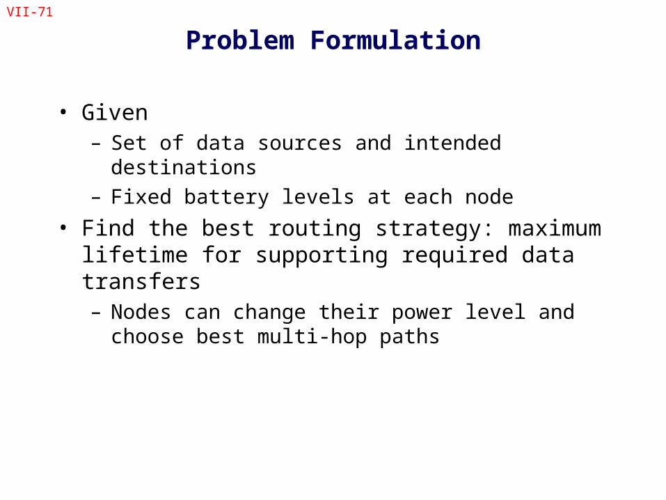
Problem Formulation
• Given – Set of data sources and intended destinations
– Fixed battery levels at each node
• Find the best routing strategy: maximum lifetime for supporting required data transfers– Nodes can change their power level and choose best
multi-hop paths
VII-72
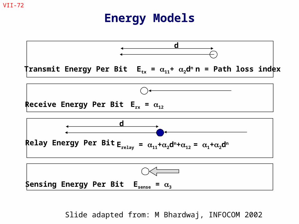
Energy Models
Etx = 11+ 2dn
d
n = Path loss index Transmit Energy Per Bit
Erx = 12Receive Energy Per Bit
Erelay = 11+2dn+12 = 1+2dn
d
Relay Energy Per Bit
Esense = 3Sensing Energy Per Bit
Slide adapted from: M Bhardwaj, INFOCOM 2002
VII-73
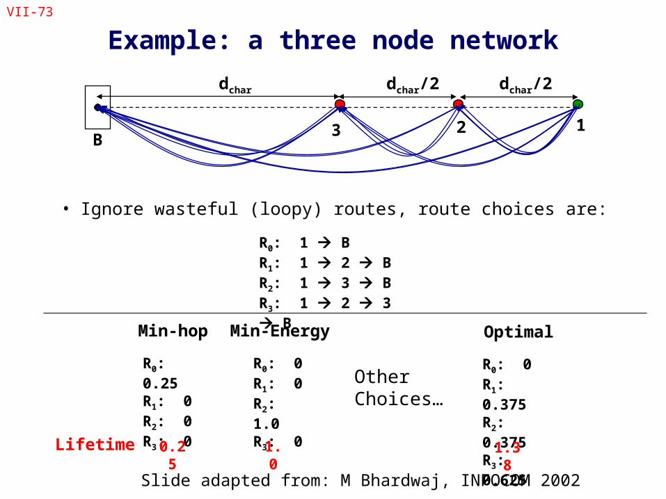
Example: a three node network
B123
dchar dchar/2 dchar/2
R0: 1 BR1: 1 2 BR2: 1 3 BR3: 1 2 3 B
Lifetime
Optimal
R0: 0R1: 0.375R2: 0.375R3: 0.625
1.38
Min-hop
R0: 0.25R1: 0R2: 0R3: 0
0.25
Min-Energy
R0: 0R1: 0R2: 1.0R3: 0
1.0
• Ignore wasteful (loopy) routes, route choices are:
Slide adapted from: M Bhardwaj, INFOCOM 2002
OtherChoices…
VII-74
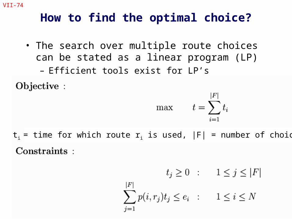
How to find the optimal choice?
• The search over multiple route choices can be stated as a linear program (LP)– Efficient tools exist for LP’s
ti = time for which route ri is used, |F| = number of choices
VII-75
Solving the LP for large networks
• The number of route choices, |F|, is exponential in number of nodes, N– LP becomes too complex for large N
• Map to a network flow problem which can be solved in polynomial time– Allows finding the optimal route choices for a given
network in polynomial time
VII-76
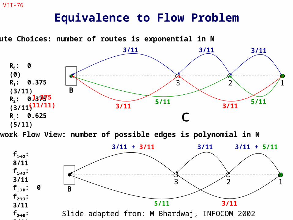
Equivalence to Flow Problem
B123
B123
R0: 0 (0)R1: 0.375 (3/11)R2: 0.375 (3/11)R3: 0.625 (5/11)
1.375 (11/11)
f12: 8/11f13: 3/11f1B: 0f23: 3/11f2B: 5/11f3B: 6/11
3/113/113/11
3/113/115/11 5/11
3/11 + 5/11
3/11
3/11
5/11
3/11 + 3/11
Route Choices: number of routes is exponential in N
Network Flow View: number of possible edges is polynomial in N
c
Slide adapted from: M Bhardwaj, INFOCOM 2002
VII-77
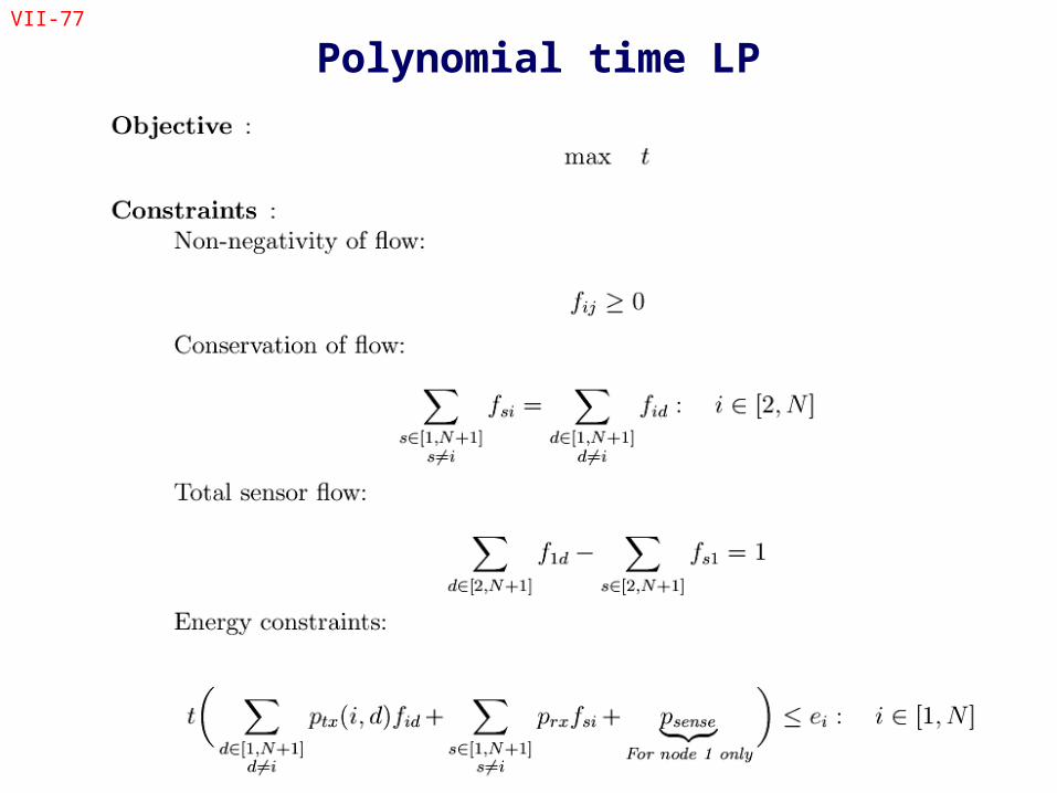
Polynomial time LP
VII-78
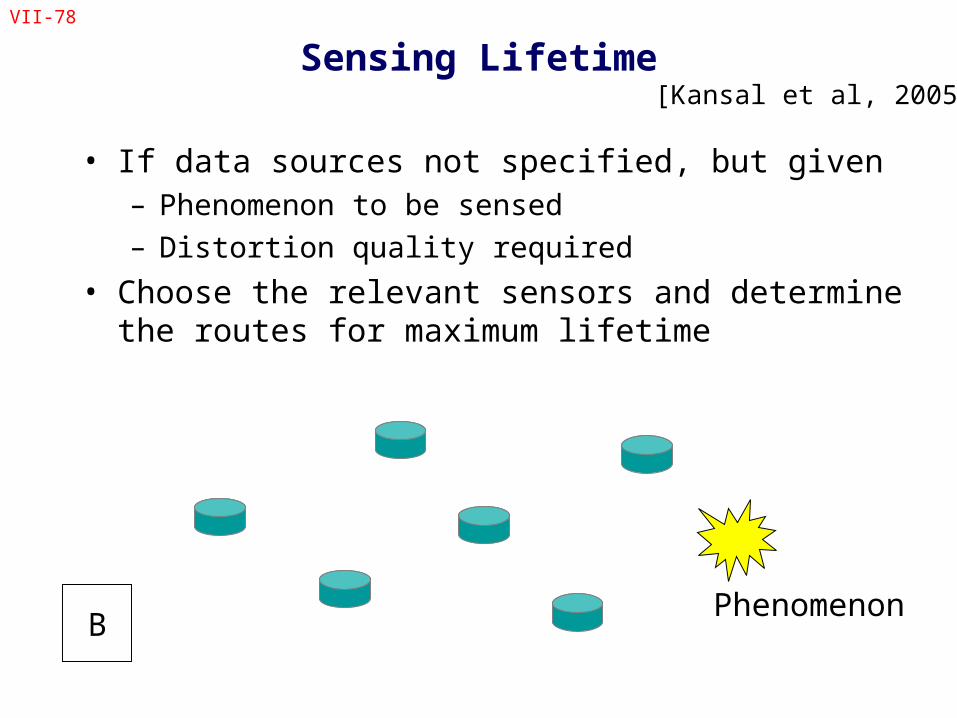
Sensing Lifetime
• If data sources not specified, but given– Phenomenon to be sensed
– Distortion quality required
• Choose the relevant sensors and determine the routes for maximum lifetime
BPhenomenon
[Kansal et al, 2005]
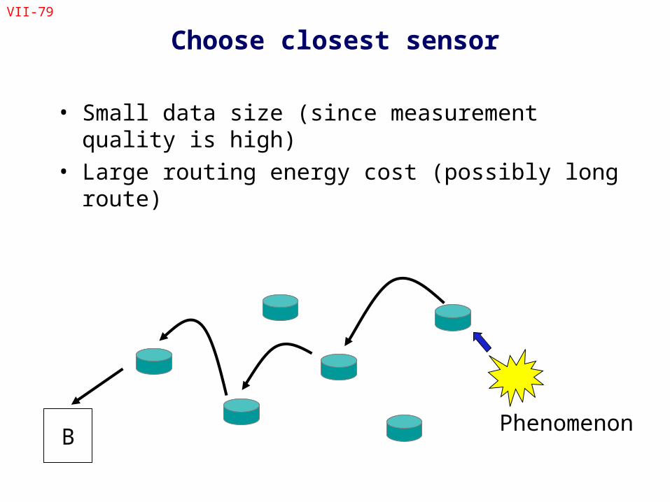
VII-79
Choose closest sensor
• Small data size (since measurement quality is high)• Large routing energy cost (possibly long route)
BPhenomenon
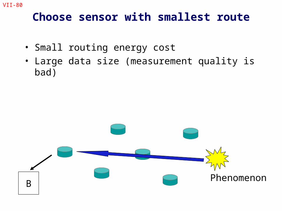
VII-80
Choose sensor with smallest route
• Small routing energy cost• Large data size (measurement quality is bad)
BPhenomenon
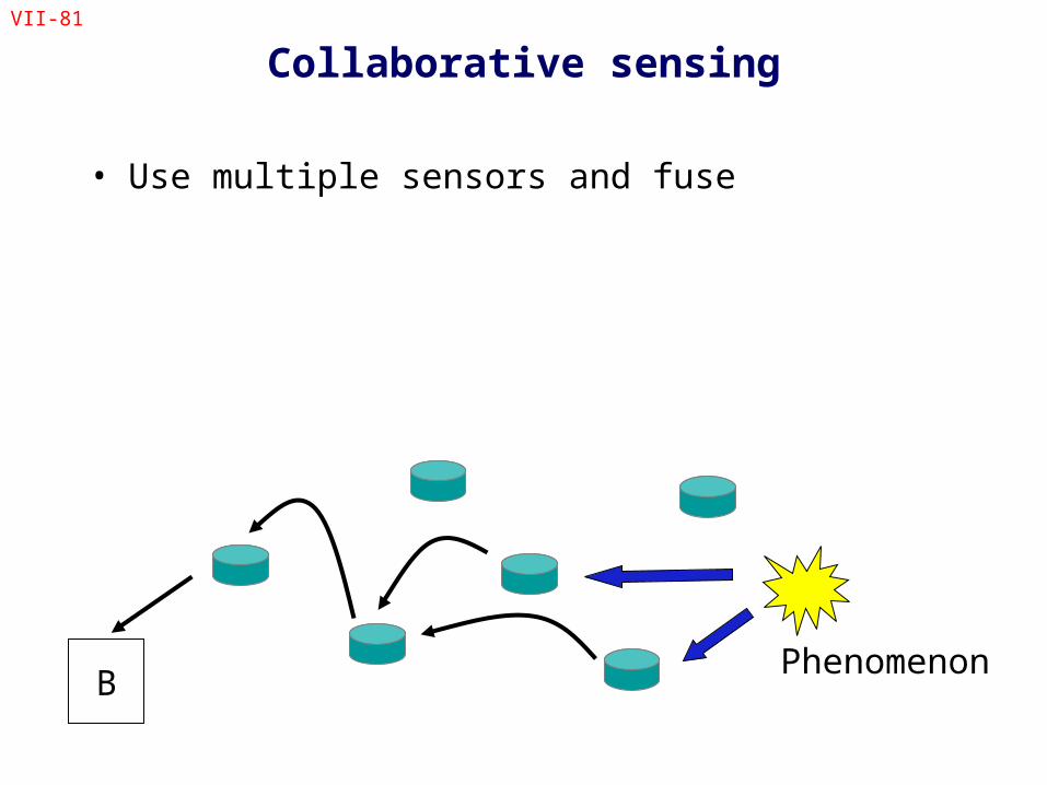
VII-81
Collaborative sensing
• Use multiple sensors and fuse
BPhenomenon
VII-82
Lifetime-Distortion Relationship
• How to determine the best choice?– Combine lifetime maximization tools with data fusion
analysis
• Find the possible choices of sensors for required distortion performance– Using data fusion analysis
• For each choice, find maximum achievable lifetime– using network flow LP
• Choose the sensors and routes which maximize lifetime
VII-83
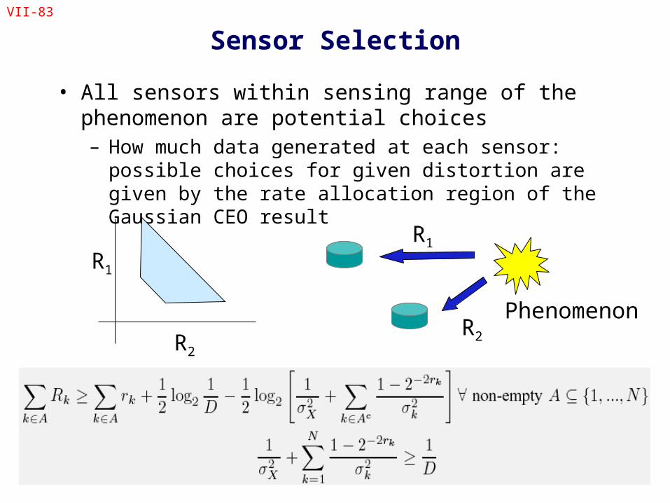
Sensor Selection
• All sensors within sensing range of the phenomenon are potential choices– How much data generated at each sensor: possible
choices for given distortion are given by the rate allocation region of the Gaussian CEO result
Phenomenon
R1
R2R2
R1
VII-84
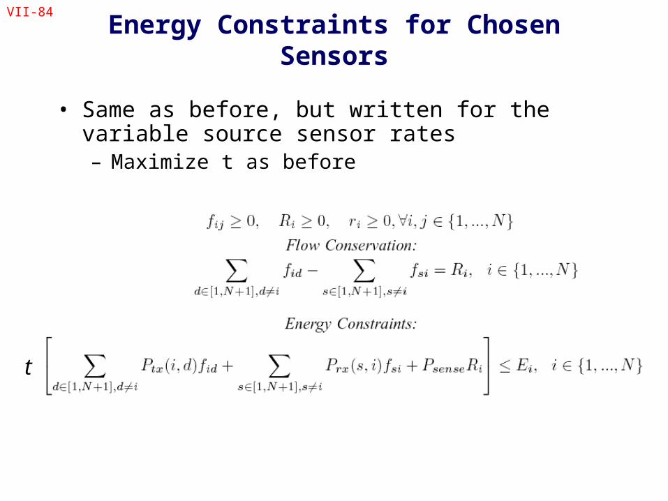
Energy Constraints for Chosen Sensors
• Same as before, but written for the variable source sensor rates– Maximize t as before
t
VII-85
Conclusions
• Network design depends on multiple methods– Optimal methods sometimes yield distributed protocols
– Provide insight into the performance of available distributed methods
• Saw some examples of analytical tools that may help network design
• Open problem: Convergence of separate solutions