Vibration monitoring of a footbridge with a wireless sensor network

http://jvc.sagepub.com/Journal of Vibration and Control

http://jvc.sagepub.com/content/19/15/2285The online version of this article can be found at:

DOI: 10.1177/1077546313501929

2013 19: 2285 originally published online 10 September 2013Journal of Vibration and ControlGlauco Feltrin, Khash Erdene Jalsan and Kallirroi Flouri

Vibration monitoring of a footbridge with a wireless sensor network

Published by:

http://www.sagepublications.com

can be found at:Journal of Vibration and ControlAdditional services and information for

http://jvc.sagepub.com/cgi/alertsEmail Alerts:

http://jvc.sagepub.com/subscriptionsSubscriptions:

http://www.sagepub.com/journalsReprints.navReprints:

http://www.sagepub.com/journalsPermissions.navPermissions:

http://jvc.sagepub.com/content/19/15/2285.refs.htmlCitations:

What is This?

- Sep 10, 2013OnlineFirst Version of Record

- Oct 11, 2013Version of Record >>

at TEXAS SOUTHERN UNIVERSITY on November 20, 2014jvc.sagepub.comDownloaded from at TEXAS SOUTHERN UNIVERSITY on November 20, 2014jvc.sagepub.comDownloaded from

http://jvc.sagepub.com/

http://jvc.sagepub.com/content/19/15/2285

http://www.sagepublications.com

http://jvc.sagepub.com/cgi/alerts

http://jvc.sagepub.com/subscriptions

http://www.sagepub.com/journalsReprints.nav

http://www.sagepub.com/journalsPermissions.nav

http://jvc.sagepub.com/content/19/15/2285.refs.html

http://jvc.sagepub.com/content/19/15/2285.full.pdf

http://jvc.sagepub.com/content/early/2013/09/10/1077546313501929.full.pdf

http://online.sagepub.com/site/sphelp/vorhelp.xhtml



Article

Vibration monitoring of a footbridgewith a wireless sensor network

Glauco Feltrin, Khash Erdene Jalsan and Kallirroi Flouri

Abstract

Monitoring the vibration performance of structures for serviceability assessment purposes usually requires a deployment

of several weeks or months to collect a dataset allowing a reliable assessment. Since for this type of medium term

deployments installation costs are a key factor, wireless monitoring with its fast deployment has an advantage over wired

monitoring systems. This paper describes a deployment of a wireless monitoring system on a timber footbridge. The goal

of the monitoring was to provide information about vibration amplitudes during operation and to track changes of

relevant natural frequencies with the temperature. Accelerations were permanently recorded and the acquired data

was processed in the nodes to compute the envelope of the vibration amplitude and the dominant peaks of the Fourier

spectrum. The wireless monitoring system that was deployed for one year provided accurate data matching the require-

ments of vibration performance assessments. The deployment demonstrated that a wireless sensor network is a tech-

nically feasible and economically effective mean to monitor the vibration performance of a structure.

Keywords

Wireless sensor network, embedded data processing, vibration monitoring, vibration serviceability

1. Introduction

Excessive vibration of a civil structure such as foot-bridges, floors etc. may produce discomfort for theusers and, as a consequence, may cause restricted useor costly retrofitting. By far the most famous case ofexcessive vibrations of recent years was the MillenniumBridge in London, which, under crowd loading on itsopening day, exhibited such high lateral vibrations thatthe bridge had to be immediately closed for retrofitting(Dallard et al., 2001). Engineering practice countsmany cases of structures that need to be assessedbecause users have complained about unpleasant vibra-tions. The current practice of vibration serviceabilityassessment is to perform vibration measurements toassess natural frequencies and vibration amplitudesunder specific loading conditions (e.g. one or two ped-estrians walking on a footbridge) and within a limitedtime period (mainly a few hours). Vibration serviceabil-ity assessment is performed by comparing the measure-ment results to natural frequencies and vibrationamplitude bounds that are specified in design codesand that should not be exceeded to guarantee anunproblematic usage of a footbridge. These tolerablevibration amplitudes, which are defined in national orinternational codes, generally depend on the vibration

frequency and vary significantly between the guidelines(Zivanovic et al., 2005; Casciati et al., 2013). However,as pointed out by Zivanovic and Pavic (2009), thesetolerable vibration amplitudes are usually not basedon experiments with footbridges and are supposed torepresent either the vibration perception of an averageperson or upper limit of acceptability by persons.Therefore, these limits consider only roughly the greatvariation of vibration perception by humans. However,not only is the vibration perception of humans charac-terized by significant randomness, but also the excita-tion process induced by pedestrians. Step frequency,step length, walking speed, and, obviously, bodyweight vary significantly between individuals (Racicet al., 2009). Furthermore, the arrival time andthus the number of pedestrians on a bridge at aparticular time is genuinely non-deterministic

Empa – Swiss Federal Laboratories for Materials Science and Technology,

Duebendorf, Switzerland

Corresponding author:

Glauco Feltrin, Empa – Swiss Federal Laboratories for Materials Science

and Technology, Ueberlandstrasse 129, 8600 Duebendorf, Switzerland.

Email: [email protected]

Received: 15 July 2013; accepted: 15 July 2013

Journal of Vibration and Control

19(15) 2285–2300

! The Author(s) 2013

Reprints and permissions:

sagepub.co.uk/journalsPermissions.nav

DOI: 10.1177/1077546313501929

jvc.sagepub.com

at TEXAS SOUTHERN UNIVERSITY on November 20, 2014jvc.sagepub.comDownloaded from


(Matsumoto et al., 1978; Zivanovic, 2012). Because ofthese widely accepted facts, the current practice of apurely deterministic approach for vibration serviceabil-ity assessments of footbridges is highly questionable.

Only recently attempts have been made to developprobabilistic concepts for defining vibration serviceabil-ity. Based on observations of the perception of pedes-trians to the vibrations amplitudes of a pedestrianbridge, Kasperski (2006) developed a serviceability cri-terion for pedestrians exposed to vibrations. He pro-posed a tentative serviceability limit state of 1s rootmean square (RMS) value of accelerations, that is 2.5time lower than the limit of the guideline ISO 10137(International Organization for Standardization,2007), the most recent code in this area. By interviewingpedestrians about the vibration perceived duringnormal traffic on a lively footbridge, Zivanovic andPavic, (2009) proposed a serviceability criterion basedon a conditional probability function that allows toestimate the percentage of people feeling unhappyduring the usage of a footbridge.

Reliable vibration serviceability criteria need to beset on a solid basis of measurements on footbridgesunder operational conditions. To fully penetrate theprobabilistic character, these measurements have tobe performed over a sufficiently long period of time.Until now, however, very few investigations addressedlong term monitoring of footbridges. Recently, Huet al. (2012a,b) presented two studies on vibrationmonitoring of two footbridges. Their main goal wasto investigate the variation of modal parametersinduced by temperature and pedestrian traffic as wellas to develop a methodology for damage detectionbeing able to cope with these variations. Caetanoet al. (2010) reported about the vibration monitoringof a footbridge for assessing the performance of tunedmass dampers. The serviceability of the footbridge wasrated on the basis of peak daily accelerations recordedover the period of a year.

In these studies, monitoring was performed withconventional wired instrumentation. The vibrationdata was recorded permanently with a fixed samplingrate and stored in a back-end server. Wired monitoringsystems are reliable, accurate, but costly in terms ofinstrumentation and deployment. In the past decade,wireless sensor networks (WSNs) have emerged as analternative structural monitoring tool. Vibration moni-toring with a WSN is particularly favorable because theacceleration sensor can be placed into the housing ofthe WSN node, which allows simplifying and accelerat-ing the mounting process on the structure.

Furthermore, vibration sensing with low powerMEMS acceleration sensors contributes in reducingenergy consumption, which is a major issue when oper-ating WSNs (Casciati et al., 2012). A summary review

of early investigations with MEMS accelerometers isprovided by Lynch and Loh (2006). Although, interms of performance low power MEMS accelerom-eters are inferior compared to high end piezo orforce-balanced accelerometers, the data quality wasgenerally rated as good provided that the vibrationamplitude was sufficiently large.

Vibration serviceability monitoring requires a per-manent sensing and data acquisition. A transfer of allthe acquired raw data by wireless communication, how-ever, is expensive in terms of power consumption. Inaddition, because of the limited bandwidth, the wirelesstransfer of the raw data would congest the communi-cation channel and produce data loss and frequent dataretransmission. Under these conditions, vibrationmonitoring periods lasting several weeks or monthswould be hardly feasible. To achieve such deploymentperiods the raw data needs to be processed in the nodeswith the goal to reduce the amount of data for trans-mission. Since in general data processing requires lessenergy than data transmission, the battery replacementperiod of a node can be extended. Signal processingalgorithms like FFT, auto regressive filters etc. weresuccessfully implemented and tested in Lynch et al.(2003) and Feltrin et al. (2006). In a long term fieldtest, the feasibility of replacement periods of severalmonths has been demonstrated (Feltrin et al., 2010).

This study explores the performance of a WSN forvibration serviceability monitoring of civil structures.The monitoring which lasted for more than a year,aimed to investigate the influence of temperaturechanges on natural frequencies and vibration ampli-tudes. The ambient as well as the pedestrian inducedvibrations of the footbridge were recorded permanentlyand natural frequencies as well as the envelope of vibra-tion amplitudes were computed by embedded data pro-cessing. Finally, the energy consumption of each nodewas monitored to identify when to replace batteries andinvestigate the reliability of the WSN monitoring sytemby analyzing the arrival rate of periodically generateddata.

2. Embedded data processing

2.1. Natural frequencies estimation

Many methods exist for estimating natural frequenciesfrom vibration records. Most of them, however, are notsuitable for WSNs due to the limited data storage andprocessing resources of wireless nodes. The best inves-tigated approach for embedded identification of naturalfrequencies is to perform an automated peak picking ofa frequency spectrum. The latter is usually achieved bycomputing the Fourier spectrum using a radix 2 imple-mentation of the fast Fourier transform (FFT)

2286 Journal of Vibration and Control 19(15)



algorithm. Peak picking is not unproblematic since it isusually done manually and therefore a certain degree ofsubjectivity is expected. Lynch et al. (2006) implementeda peak picking algorithm for automated modal shapeestimation. The modal frequency estimation algorithmwas successfully applied and tested for estimating oper-ational mode shapes of a road bridge. Zimmerman et al.(2008) improved this algorithm by transmitting themodal frequencies estimates of each sensor node to thebase station. Based on these individual estimates, thebase station then computed an improved estimate ofthe natural frequencies that were eventually broadcastedback to the sensor nodes for mode shape computation.This approach allowed reducing the scattering of auto-mated peak picking. These investigations, however, didnot specify any details about the implementation of theautomated peak picking algorithm.

An automated peak picking algorithm was proposedby Lei et al. (2010). They scanned the frequency spec-trum for values that were greater than a given thresholdvalue and their neighboring values. The threshold,which had to be carefully assigned, was introduced toeliminate small spurious peaks, while keeping the non-spurious peaks in the frequency spectrum. The fre-quency estimation algorithm was tested on the hangersof an arch bridge.

Autoregressive (AR) filters have also been used forestimating natural frequencies (Feltrin et al., 2006;2010). Autoregressive filters have a significant advan-tage compared to FFT-based spectral methods sincethey need much less raw data. However, computingthe coefficients of AR filters requires floating pointoperations. Since the low power microcontroller imple-mented in WSNs usually does not support hardwarefloating point operations, these operations have to beemulated with integer operations resulting in a greatercode size and long execution time (Feltrin et al., 2010).

In this work the authors propose a new algorithmfor estimating natural frequencies by peak picking. Itdiffers from the work described above by a fast imple-mentation of the FFT and a new peak picking algo-rithm. The natural frequencies estimation isperformed in six steps and fits very well into the conceptof a data processing pipeline.

1. The raw data, which was acquired with a depth of12 bit and stored in 16 bit words, was scaled to fullyexploit the range (�215, 215] with the goal to minim-ize precision loss during the data processing and inparticular when performing the FFT.

2. The complex Fourier coefficients of the scaled vibra-tion record are computed using a radix 2 FFT algo-rithm. Since microcontrollers do not supporthardware floating point operations, the FFT algo-rithm was implemented using fixed point operations.

The algorithm turned out to be 10 times faster thanthe same algorithm executed using floating pointoperations. As a consequence, the power consump-tion required for the data processing as well as thecode size could be decreased, thus increasing thepower efficiency of a node. To avoid arithmetic over-flow in multiplication operations, the two 16 bit inte-ger operands are processed to obtain a 32 bit result.For further processing only the higher 16 bits arekept, i.e. the lower 16 bits of the result are discarded.Such an approximation mechanism may introducean error when compared to a floating point FFTimplementation. The scaling of the vibrationrecord performed in the first processing step, how-ever, significantly reduces the approximation error.Furthermore, since only isolated peaks of the spec-trum are of interest, small approximation errorshave very limited effects on the accuracy of naturalfrequency estimation.

3. Next, the frequency spectrum is computed by takingthe absolute values of the complex Fouriercoefficients.

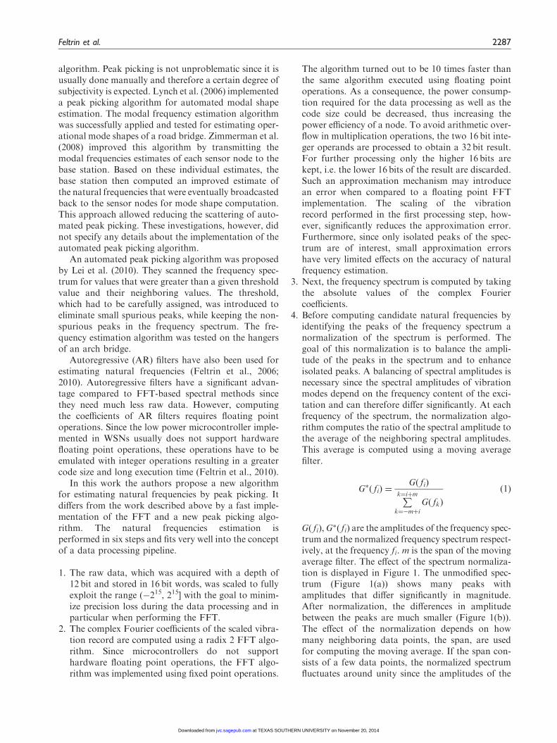
4. Before computing candidate natural frequencies byidentifying the peaks of the frequency spectrum anormalization of the spectrum is performed. Thegoal of this normalization is to balance the ampli-tude of the peaks in the spectrum and to enhanceisolated peaks. A balancing of spectral amplitudes isnecessary since the spectral amplitudes of vibrationmodes depend on the frequency content of the exci-tation and can therefore differ significantly. At eachfrequency of the spectrum, the normalization algo-rithm computes the ratio of the spectral amplitude tothe average of the neighboring spectral amplitudes.This average is computed using a moving averagefilter.

G�ð fiÞ ¼Gð fiÞ

Pk¼iþm

k¼�mþi

Gð fkÞ

ð1Þ

Gð fiÞ,G�ð fiÞ are the amplitudes of the frequency spec-

trum and the normalized frequency spectrum respect-ively, at the frequency fi. m is the span of the movingaverage filter. The effect of the spectrum normaliza-tion is displayed in Figure 1. The unmodified spec-trum (Figure 1(a)) shows many peaks withamplitudes that differ significantly in magnitude.After normalization, the differences in amplitudebetween the peaks are much smaller (Figure 1(b)).The effect of the normalization depends on howmany neighboring data points, the span, are usedfor computing the moving average. If the span con-sists of a few data points, the normalized spectrumfluctuates around unity since the amplitudes of the

Feltrin et al. 2287



data points in the immediate neighborhood are com-parable to the amplitude of the center frequency.Very large spans generate a normalized spectrumthat is very similar to the original spectrum sincethe variations of the moving average diminish whilethe span increases.

5. The fifth data processing step consists in computinglocal minima and maxima of the normalized spec-trum. In order to avoid identifying irrelevant minimaand maxima, the amplitude difference betweensubsequent extrema G�ð fiÞ and G�ð fj Þ, a local min-imum and maximum, must exceed a pre-definedthreshold �:

G�ð fiÞ � G�ð fj Þ��

��4�: ð2Þ

This threshold helps also to compact neighboringpeaks that are separated by a single minimum to asingle peak. Such a situation occurs quite often inthe spectrum of a vibration record.

6. The final processing step consists in searching thearray for identifying the N frequencies having thelargest spectral amplitude.

The processing time of the different steps on aMSP430F1611 microcontroller are summarized inTable 1. For an array with 1024 samples the total com-putation time is 2.81 s. The most time consuming dataprocessing step is the normalization of the spectrumthat takes 1.81 s because it has to be performed usingfloating point operations. All other algorithms areimplemented in fixed point operations. The most com-plex algorithm, the FFT algorithm, is therefore veryfast and takes only 0.54 s to complete.

The embedded algorithm does not perform any aver-aging of the Fourier spectra. Averaging of

periodograms is a well-established technique toimprove the estimation of the spectrum since it reducesthe effect of randomness in the spectrum. Because ofthe limited data storage capabilities, however, aver-aging is cumbersome and inefficient to implement in aWSN node. Because of the noisy spectrum, the frequen-cies selected by peak picking are subjected to a signifi-cant scattering. Therefore, a single frequency estimatemay be inaccurate. However, by calculating the averageof a large sample of such single record estimates a moreaccurate estimate of natural frequencies can beexpected. This post-processing can be done effectivelyat the backend, thus reducing the complexity of theWSN node software.

2.2. Vibration amplitudes

Vibration assessment of civil structures is usually basedon limit values of vibration amplitudes. These limitvalues are often defined as peak amplitudes or asRMS of the vibration amplitudes. In the context of aprobabilistic vibration assessment framework, theselimit values would be defined as a threshold thatshould not be exceeded with a given probabilitywithin a certain period of time. Therefore, for vibrationassessment purposes, monitoring only the peak ampli-tudes or the RMS of vibration amplitudes would besufficient.

Peak or RMS amplitudes are computed by analyzingthe recorded vibrations within a given time interval.While for peak amplitudes the time interval is usuallyundefined, the guideline ISO 10137 (InternationalOrganization for Standardization, 2007) specifies a 1 stime interval for the computation of the RMS.

Embedded computing peak or RMS amplitudes canbe performed quite efficiently with a microprocessor. Itis also an effective mean to significantly reduce the datasize for transmission. The ratio of the resulting reduceddata size to the original data size is inversely

0 5 10 150

0.01

0.02

0.03

0.04

0.05

frequency [Hz]

spec

trum

[m

s−2 ]

0 5 10 150

1

2

3

4

5

frequency [Hz]

norm

aliz

ed s

pect

rum

(a) (b)

Figure 1. (a) Original spectrum and (b) normalized spectrum with a span of 41.




proportional to the sampling period of data acquisitionand the time interval of peak and RMS evaluation.With a sampling frequency of 50Hz and time intervalof 1 s only 2% of the original data size has to betransmitted.

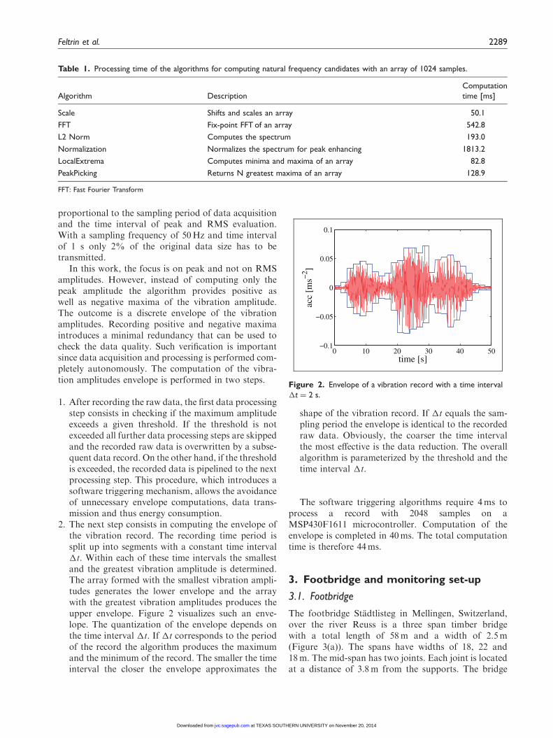
In this work, the focus is on peak and not on RMSamplitudes. However, instead of computing only thepeak amplitude the algorithm provides positive aswell as negative maxima of the vibration amplitude.The outcome is a discrete envelope of the vibrationamplitudes. Recording positive and negative maximaintroduces a minimal redundancy that can be used tocheck the data quality. Such verification is importantsince data acquisition and processing is performed com-pletely autonomously. The computation of the vibra-tion amplitudes envelope is performed in two steps.

1. After recording the raw data, the first data processingstep consists in checking if the maximum amplitudeexceeds a given threshold. If the threshold is notexceeded all further data processing steps are skippedand the recorded raw data is overwritten by a subse-quent data record. On the other hand, if the thresholdis exceeded, the recorded data is pipelined to the nextprocessing step. This procedure, which introduces asoftware triggering mechanism, allows the avoidanceof unnecessary envelope computations, data trans-mission and thus energy consumption.

2. The next step consists in computing the envelope ofthe vibration record. The recording time period issplit up into segments with a constant time interval�t. Within each of these time intervals the smallestand the greatest vibration amplitude is determined.The array formed with the smallest vibration ampli-tudes generates the lower envelope and the arraywith the greatest vibration amplitudes produces theupper envelope. Figure 2 visualizes such an enve-lope. The quantization of the envelope depends onthe time interval �t. If �t corresponds to the periodof the record the algorithm produces the maximumand the minimum of the record. The smaller the timeinterval the closer the envelope approximates the

shape of the vibration record. If �t equals the sam-pling period the envelope is identical to the recordedraw data. Obviously, the coarser the time intervalthe most effective is the data reduction. The overallalgorithm is parameterized by the threshold and thetime interval �t.

The software triggering algorithms require 4ms toprocess a record with 2048 samples on aMSP430F1611 microcontroller. Computation of theenvelope is completed in 40ms. The total computationtime is therefore 44ms.

3. Footbridge and monitoring set-up

3.1. Footbridge

The footbridge Stadtlisteg in Mellingen, Switzerland,over the river Reuss is a three span timber bridgewith a total length of 58m and a width of 2.5m(Figure 3(a)). The spans have widths of 18, 22 and18m. The mid-span has two joints. Each joint is locatedat a distance of 3.8m from the supports. The bridge

Table 1. Processing time of the algorithms for computing natural frequency candidates with an array of 1024 samples.

Algorithm Description

Computation

time [ms]

Scale Shifts and scales an array 50.1

FFT Fix-point FFT of an array 542.8

L2 Norm Computes the spectrum 193.0

Normalization Normalizes the spectrum for peak enhancing 1813.2

LocalExtrema Computes minima and maxima of an array 82.8

PeakPicking Returns N greatest maxima of an array 128.9

FFT: Fast Fourier Transform

0 10 20 30 40 50−0.1

−0.05

0

0.05

0.1

acc

[ms−

2 ]

time [s]

Figure 2. Envelope of a vibration record with a time interval

�t ¼ 2 s.

Feltrin et al. 2289



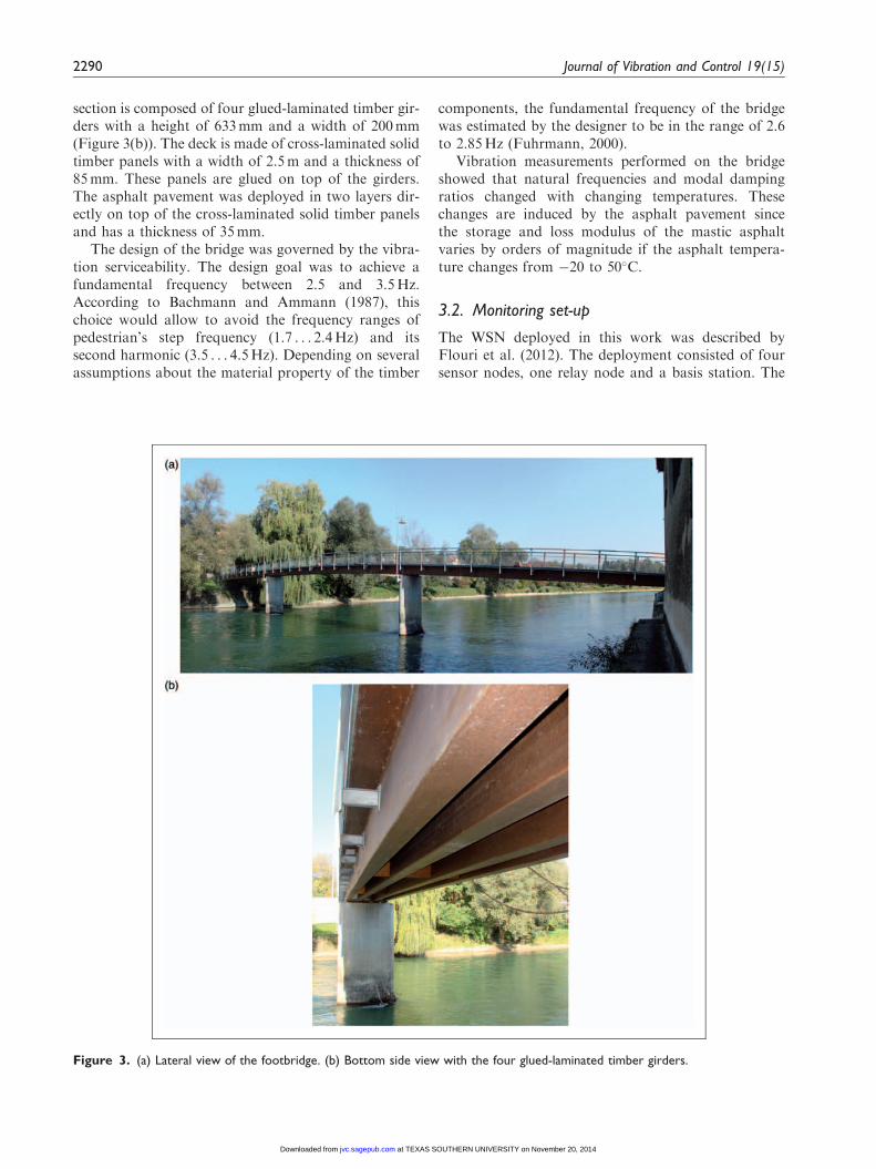
section is composed of four glued-laminated timber gir-ders with a height of 633mm and a width of 200mm(Figure 3(b)). The deck is made of cross-laminated solidtimber panels with a width of 2.5m and a thickness of85mm. These panels are glued on top of the girders.The asphalt pavement was deployed in two layers dir-ectly on top of the cross-laminated solid timber panelsand has a thickness of 35mm.

The design of the bridge was governed by the vibra-tion serviceability. The design goal was to achieve afundamental frequency between 2.5 and 3.5Hz.According to Bachmann and Ammann (1987), thischoice would allow to avoid the frequency ranges ofpedestrian’s step frequency (1.7 . . . 2.4Hz) and itssecond harmonic (3.5 . . . 4.5Hz). Depending on severalassumptions about the material property of the timber

components, the fundamental frequency of the bridgewas estimated by the designer to be in the range of 2.6to 2.85Hz (Fuhrmann, 2000).

Vibration measurements performed on the bridgeshowed that natural frequencies and modal dampingratios changed with changing temperatures. Thesechanges are induced by the asphalt pavement sincethe storage and loss modulus of the mastic asphaltvaries by orders of magnitude if the asphalt tempera-ture changes from �20 to 50�C.

3.2. Monitoring set-up

The WSN deployed in this work was described byFlouri et al. (2012). The deployment consisted of foursensor nodes, one relay node and a basis station. The

Figure 3. (a) Lateral view of the footbridge. (b) Bottom side view with the four glued-laminated timber girders.




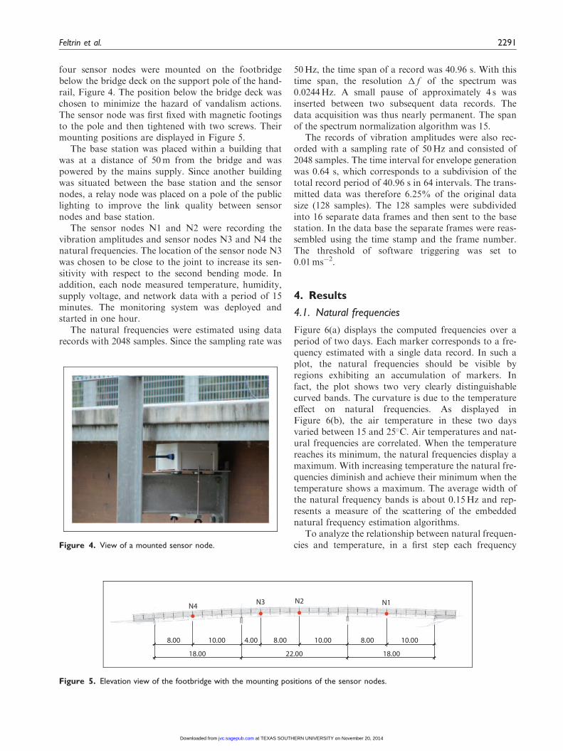
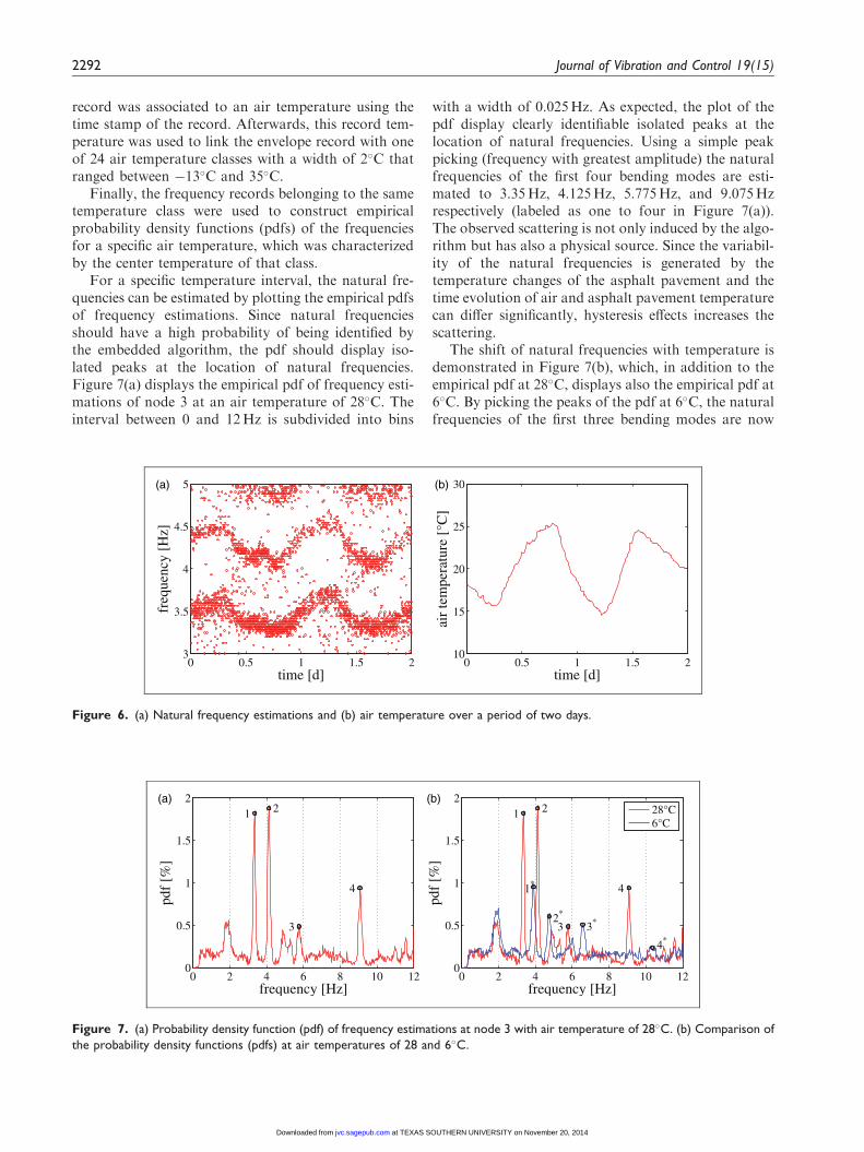
four sensor nodes were mounted on the footbridgebelow the bridge deck on the support pole of the hand-rail, Figure 4. The position below the bridge deck waschosen to minimize the hazard of vandalism actions.The sensor node was first fixed with magnetic footingsto the pole and then tightened with two screws. Theirmounting positions are displayed in Figure 5.

The base station was placed within a building thatwas at a distance of 50m from the bridge and waspowered by the mains supply. Since another buildingwas situated between the base station and the sensornodes, a relay node was placed on a pole of the publiclighting to improve the link quality between sensornodes and base station.

The sensor nodes N1 and N2 were recording thevibration amplitudes and sensor nodes N3 and N4 thenatural frequencies. The location of the sensor node N3was chosen to be close to the joint to increase its sen-sitivity with respect to the second bending mode. Inaddition, each node measured temperature, humidity,supply voltage, and network data with a period of 15minutes. The monitoring system was deployed andstarted in one hour.

The natural frequencies were estimated using datarecords with 2048 samples. Since the sampling rate was

50Hz, the time span of a record was 40.96 s. With thistime span, the resolution � f of the spectrum was0.0244Hz. A small pause of approximately 4 s wasinserted between two subsequent data records. Thedata acquisition was thus nearly permanent. The spanof the spectrum normalization algorithm was 15.

The records of vibration amplitudes were also rec-orded with a sampling rate of 50Hz and consisted of2048 samples. The time interval for envelope generationwas 0.64 s, which corresponds to a subdivision of thetotal record period of 40.96 s in 64 intervals. The trans-mitted data was therefore 6.25% of the original datasize (128 samples). The 128 samples were subdividedinto 16 separate data frames and then sent to the basestation. In the data base the separate frames were reas-sembled using the time stamp and the frame number.The threshold of software triggering was set to0.01ms�2.

4. Results

4.1. Natural frequencies

Figure 6(a) displays the computed frequencies over aperiod of two days. Each marker corresponds to a fre-quency estimated with a single data record. In such aplot, the natural frequencies should be visible byregions exhibiting an accumulation of markers. Infact, the plot shows two very clearly distinguishablecurved bands. The curvature is due to the temperatureeffect on natural frequencies. As displayed inFigure 6(b), the air temperature in these two daysvaried between 15 and 25�C. Air temperatures and nat-ural frequencies are correlated. When the temperaturereaches its minimum, the natural frequencies display amaximum. With increasing temperature the natural fre-quencies diminish and achieve their minimum when thetemperature shows a maximum. The average width ofthe natural frequency bands is about 0.15Hz and rep-resents a measure of the scattering of the embeddednatural frequency estimation algorithms.

To analyze the relationship between natural frequen-cies and temperature, in a first step each frequency

22.0018.00 18.00

8.00 10.00 10.008.008.00 10.00

N4N2 N1N3

4.00

Figure 5. Elevation view of the footbridge with the mounting positions of the sensor nodes.

Figure 4. View of a mounted sensor node.

Feltrin et al. 2291



record was associated to an air temperature using thetime stamp of the record. Afterwards, this record tem-perature was used to link the envelope record with oneof 24 air temperature classes with a width of 2�C thatranged between �13�C and 35�C.

Finally, the frequency records belonging to the sametemperature class were used to construct empiricalprobability density functions (pdfs) of the frequenciesfor a specific air temperature, which was characterizedby the center temperature of that class.

For a specific temperature interval, the natural fre-quencies can be estimated by plotting the empirical pdfsof frequency estimations. Since natural frequenciesshould have a high probability of being identified bythe embedded algorithm, the pdf should display iso-lated peaks at the location of natural frequencies.Figure 7(a) displays the empirical pdf of frequency esti-mations of node 3 at an air temperature of 28�C. Theinterval between 0 and 12Hz is subdivided into bins

with a width of 0.025Hz. As expected, the plot of thepdf display clearly identifiable isolated peaks at thelocation of natural frequencies. Using a simple peakpicking (frequency with greatest amplitude) the naturalfrequencies of the first four bending modes are esti-mated to 3.35Hz, 4.125Hz, 5.775Hz, and 9.075Hzrespectively (labeled as one to four in Figure 7(a)).The observed scattering is not only induced by the algo-rithm but has also a physical source. Since the variabil-ity of the natural frequencies is generated by thetemperature changes of the asphalt pavement and thetime evolution of air and asphalt pavement temperaturecan differ significantly, hysteresis effects increases thescattering.

The shift of natural frequencies with temperature isdemonstrated in Figure 7(b), which, in addition to theempirical pdf at 28�C, displays also the empirical pdf at6�C. By picking the peaks of the pdf at 6�C, the naturalfrequencies of the first three bending modes are now

0 2 4 6 8 10 120

0.5

1

1.5

21 2

3

4

frequency [Hz]

pdf

[%]

0 2 4 6 8 10 120

0.5

1

1.5

2

1*

2*

3*

4*

1 2

3

4

frequency [Hz]

pdf

[%]

28°C6°C

(a) (b)

Figure 7. (a) Probability density function (pdf) of frequency estimations at node 3 with air temperature of 28�C. (b) Comparison of

the probability density functions (pdfs) at air temperatures of 28 and 6�C.

0 0.5 1 1.5 23

3.5

4

4.5

5

time [d]

freq

uenc

y [H

z]

0 0.5 1 1.5 210

15

20

25

30

time [d]

air

tem

pera

ture

[°C

]

(a) (b)

Figure 6. (a) Natural frequency estimations and (b) air temperature over a period of two days.




3.90Hz, 4.75Hz, and 6.575Hz respectively (labeled asone to three in Figure 7(b)).

The natural frequency of the fourth bending mode isonly identifiable by tracking its variation with tempera-ture since its peak amplitude shrinks significantly withdecreasing temperature. At 6�C, its natural frequencywas estimated to be 10.3Hz (Figure 7(b)).

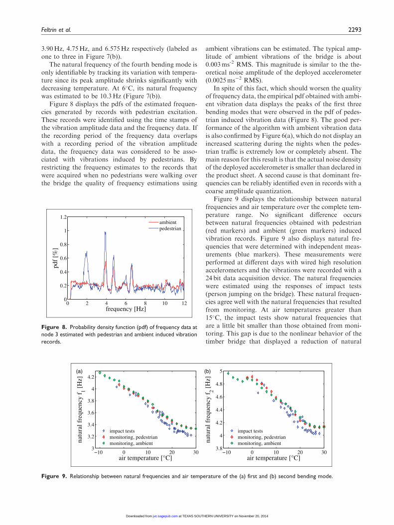
Figure 8 displays the pdfs of the estimated frequen-cies generated by records with pedestrian excitation.These records were identified using the time stamps ofthe vibration amplitude data and the frequency data. Ifthe recording period of the frequency data overlapswith a recording period of the vibration amplitudedata, the frequency data was considered to be asso-ciated with vibrations induced by pedestrians. Byrestricting the frequency estimates to the records thatwere acquired when no pedestrians were walking overthe bridge the quality of frequency estimations using

ambient vibrations can be estimated. The typical amp-litude of ambient vibrations of the bridge is about0.003ms-2 RMS. This magnitude is similar to the the-oretical noise amplitude of the deployed accelerometer(0.0025ms�2 RMS).

In spite of this fact, which should worsen the qualityof frequency data, the empirical pdf obtained with ambi-ent vibration data displays the peaks of the first threebending modes that were observed in the pdf of pedes-trian induced vibration data (Figure 8). The good per-formance of the algorithm with ambient vibration datais also confirmed by Figure 6(a), which do not display anincreased scattering during the nights when the pedes-trian traffic is extremely low or completely absent. Themain reason for this result is that the actual noise densityof the deployed accelerometer is smaller than declared inthe product sheet. A second cause is that dominant fre-quencies can be reliably identified even in records with acoarse amplitude quantization.

Figure 9 displays the relationship between naturalfrequencies and air temperature over the complete tem-perature range. No significant difference occursbetween natural frequencies obtained with pedestrian(red markers) and ambient (green markers) inducedvibration records. Figure 9 also displays natural fre-quencies that were determined with independent meas-urements (blue markers). These measurements wereperformed at different days with wired high resolutionaccelerometers and the vibrations were recorded with a24 bit data acquisition device. The natural frequencieswere estimated using the responses of impact tests(person jumping on the bridge). These natural frequen-cies agree well with the natural frequencies that resultedfrom monitoring. At air temperatures greater than15�C, the impact tests show natural frequencies thatare a little bit smaller than those obtained from moni-toring. This gap is due to the nonlinear behavior of thetimber bridge that displayed a reduction of natural

−10 0 10 20 303

3.2

3.4

3.6

3.8

4

4.2

air temperature [°C]

natu

ral f

requ

ency

f1 [

Hz]

impact testsmonitoring, pedestrianmonitoring, ambient

−10 0 10 20 303.8

4

4.2

4.4

4.6

4.8

5


natu

ral f

requ

ency

f2 [

Hz]

impact testsmonitoring, pedestrianmonitoring, ambient

(a) (b)

Figure 9. Relationship between natural frequencies and air temperature of the (a) first and (b) second bending mode.

0 2 4 6 8 10 120

0.2

0.4

0.6

0.8

1

1.2

frequency [Hz]

pdf

[%]

ambientpedestrian

Figure 8. Probability density function (pdf) of frequency data at

node 3 estimated with pedestrian and ambient induced vibration

records.

Feltrin et al. 2293



frequencies with increasing vibration amplitudes. Ingeneral, the impact tests generated peak vibration amp-litudes that were about five to 10 times larger than theaverage vibration amplitudes induced by pedestrians,which, as shown in the next section, were about0.08ms�2.

Figure 7(b) shows a peak of the pdf just below 2Hzthat is not sensitive to temperature changes. As dis-played in Figure 8, this peak appears in the pdf obtainedfrom pedestrian induced vibrations but it does notappear in the pdf generated by ambient vibrations. Themost likely interpretation of this peak is that it is relatedto the pace frequency of the pedestrians.

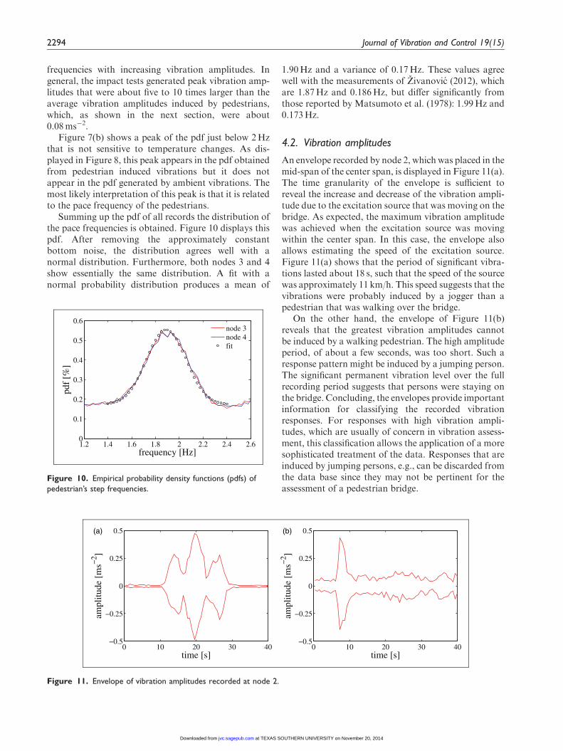
Summing up the pdf of all records the distribution ofthe pace frequencies is obtained. Figure 10 displays thispdf. After removing the approximately constantbottom noise, the distribution agrees well with anormal distribution. Furthermore, both nodes 3 and 4show essentially the same distribution. A fit with anormal probability distribution produces a mean of

1.90Hz and a variance of 0.17Hz. These values agreewell with the measurements of Zivanovic (2012), whichare 1.87Hz and 0.186Hz, but differ significantly fromthose reported by Matsumoto et al. (1978): 1.99Hz and0.173Hz.

4.2. Vibration amplitudes

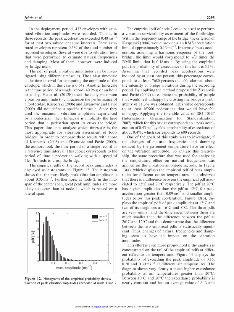
An envelope recorded by node 2, which was placed in themid-span of the center span, is displayed in Figure 11(a).The time granularity of the envelope is sufficient toreveal the increase and decrease of the vibration ampli-tude due to the excitation source that was moving on thebridge. As expected, the maximum vibration amplitudewas achieved when the excitation source was movingwithin the center span. In this case, the envelope alsoallows estimating the speed of the excitation source.Figure 11(a) shows that the period of significant vibra-tions lasted about 18 s, such that the speed of the sourcewas approximately 11 km/h. This speed suggests that thevibrations were probably induced by a jogger than apedestrian that was walking over the bridge.

On the other hand, the envelope of Figure 11(b)reveals that the greatest vibration amplitudes cannotbe induced by a walking pedestrian. The high amplitudeperiod, of about a few seconds, was too short. Such aresponse pattern might be induced by a jumping person.The significant permanent vibration level over the fullrecording period suggests that persons were staying onthe bridge. Concluding, the envelopes provide importantinformation for classifying the recorded vibrationresponses. For responses with high vibration ampli-tudes, which are usually of concern in vibration assess-ment, this classification allows the application of a moresophisticated treatment of the data. Responses that areinduced by jumping persons, e.g., can be discarded fromthe data base since they may not be pertinent for theassessment of a pedestrian bridge.

0 10 20 30 40−0.5

−0.25

0

0.25

0.5

time [s]

ampl

itude

[m

s−2 ]

0 10 20 30 40−0.5

−0.25

0

0.25

0.5

time [s]

ampl

itude

[m

s−2 ]

(a) (b)

Figure 11. Envelope of vibration amplitudes recorded at node 2.

1.2 1.4 1.6 1.8 2 2.2 2.4 2.60

0.1

0.2

0.3

0.4

0.5

0.6

frequency [Hz]

pdf

[%]

node 3node 4fit

Figure 10. Empirical probability density functions (pdfs) of

pedestrian’s step frequencies.




In the deployment period, 432 envelopes with satu-rated vibration amplitudes were recorded. That is, inthese records, the peak acceleration exceeded 0.48ms�2

for at least two subsequent time intervals. These satu-rated envelopes represent 0.3% of the total number ofrecorded envelopes. Several were due to vibration teststhat were performed to estimate natural frequenciesand damping. Most of them, however, were inducedby bridge users.

The pdf of peak vibration amplitudes can be inves-tigated using different timescales. The tiniest timescaleis the time interval for computing the amplitude of theenvelope, which in this case is 0.64 s. Another timescaleis the time period of a single record (40.96 s) or an houror a day. Hu et al. (2012b) used the daily maximumvibration amplitude to characterize the performance ofa footbridge. Kasperski (2006) and Zivanovic and Pavic(2009) did not define a specific timescale. Since theyused the maximum vibration amplitude experiencedby a pedestrian, their timescale is implicitly the timeperiod that a pedestrian spent to cross the bridge.This paper does not analyze which timescale is themost appropriate for vibration assessment of foot-bridges. In order to compare these results with thoseof Kasperski (2006) and Zivanovic and Pavic (2009),the authors took the time period of a single record asa reference time interval. This choice corresponds to theperiod of time a pedestrian walking with a speed of5 km/h needs to cross the bridge.

The empirical pdfs of the record peak amplitudes isdisplayed as histograms in Figure 12. The histogramshows that the most likely peak vibration amplitude isabout 0.05ms�2. Furthermore, at node 2, in the mid-span of the center span, great peak amplitudes are morelikely to occur than at node 1, which is placed on alateral span.

The empirical pdf of node 2 could be used to performa vibration serviceability assessment of the footbridge.Within the frequency range of the bridge, the criterion ofKasperski (2006) would provide a 1 s RMS accelerationlimit of approximately 0.13ms�2. In terms of peak accel-eration, assuming a harmonic response of the foot-bridge, the limit would correspond to

ffiffiffi2p

times theRMS limit, that is 0.18ms�2. By using the empiricalpdf, the probability of exceedance of this limit is 5.1%.Assuming that recorded peak accelerations wereinduced by at least one person, this percentage corres-ponds to at least 7680 persons that felt alarmed aboutthe intensity of bridge vibrations during the recordingperiod. By applying the method proposed by Zivanovicand Pavic (2009) to estimate the probability of peoplethat would feel unhappy by crossing the bridge a prob-ability of 11.3% was obtained. This value correspondsto at least 16’900 pedestrians that would have feltunhappy. Applying the tolerable value of ISO 10137(International Organization for Standardization,2007), which for this bridge corresponds to a peak accel-eration of 0.43ms-2, yields a probability of exceedance ofabout 0.4%, which corresponds to 600 records.

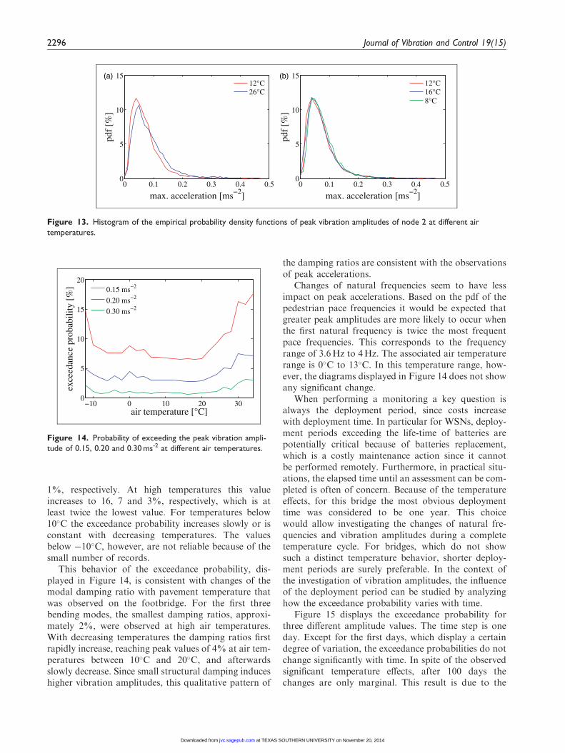
One of the goals of this study was to investigate, ifthe changes of natural frequencies and dampinginduced by the pavement temperature have an effecton the vibration amplitude. To analyze this relation-ship, the same procedure that was used for analyzingthe temperature effect on natural frequencies wasapplied on the vibration amplitude records. In Figure13(a), which displays the empirical pdf of peak ampli-tudes for different center temperatures, it is observedthat there is a difference between the empirical pdf asso-ciated to 12�C and 26�C respectively. The pdf at 26�Chas higher amplitudes than the pdf at 12�C for peakacceleration greater than 0.09ms-2 and smaller ampli-tudes below this peak acceleration. Figure 13(b), dis-plays the empirical pdfs of peak amplitudes at 12�C andtwo of its neighbors at 16�C and 8�C. The three pdfsare very similar and the differences between them aremuch smaller than the difference between the pdf at26�C and 12�C and thus demonstrate that the differencebetween the two empirical pdfs is statistically signifi-cant. Thus, changes of natural frequencies and damp-ing seem to have an impact on the vibrationamplitudes.

This effect is even more pronounced if the analysis isconcentrated on the tail of the empirical pdfs at differ-ent reference air temperatures. Figure 14 displays theprobability of exceeding the peak amplitude of 0.15,0.20 and 0.30ms�2 at different air temperatures. Thediagram shows very clearly a much higher exceedanceprobability at air temperatures greater than 20�C.Between 10�C and 20�C the exceedance probability isnearly constant and has an average value of 8, 3 and

0 0.1 0.2 0.3 0.4 0.50

2

4

6

8

10

12

pdf

[%]

max. amplitude [ms−2]

node 1node 2

Figure 12. Histograms of the empirical probability density

function of peak vibration amplitudes recorded at node 1 and 2.

Feltrin et al. 2295



1%, respectively. At high temperatures this valueincreases to 16, 7 and 3%, respectively, which is atleast twice the lowest value. For temperatures below10�C the exceedance probability increases slowly or isconstant with decreasing temperatures. The valuesbelow �10�C, however, are not reliable because of thesmall number of records.

This behavior of the exceedance probability, dis-played in Figure 14, is consistent with changes of themodal damping ratio with pavement temperature thatwas observed on the footbridge. For the first threebending modes, the smallest damping ratios, approxi-mately 2%, were observed at high air temperatures.With decreasing temperatures the damping ratios firstrapidly increase, reaching peak values of 4% at air tem-peratures between 10�C and 20�C, and afterwardsslowly decrease. Since small structural damping induceshigher vibration amplitudes, this qualitative pattern of

the damping ratios are consistent with the observationsof peak accelerations.

Changes of natural frequencies seem to have lessimpact on peak accelerations. Based on the pdf of thepedestrian pace frequencies it would be expected thatgreater peak amplitudes are more likely to occur whenthe first natural frequency is twice the most frequentpace frequencies. This corresponds to the frequencyrange of 3.6Hz to 4Hz. The associated air temperaturerange is 0�C to 13�C. In this temperature range, how-ever, the diagrams displayed in Figure 14 does not showany significant change.

When performing a monitoring a key question isalways the deployment period, since costs increasewith deployment time. In particular for WSNs, deploy-ment periods exceeding the life-time of batteries arepotentially critical because of batteries replacement,which is a costly maintenance action since it cannotbe performed remotely. Furthermore, in practical situ-ations, the elapsed time until an assessment can be com-pleted is often of concern. Because of the temperatureeffects, for this bridge the most obvious deploymenttime was considered to be one year. This choicewould allow investigating the changes of natural fre-quencies and vibration amplitudes during a completetemperature cycle. For bridges, which do not showsuch a distinct temperature behavior, shorter deploy-ment periods are surely preferable. In the context ofthe investigation of vibration amplitudes, the influenceof the deployment period can be studied by analyzinghow the exceedance probability varies with time.

Figure 15 displays the exceedance probability forthree different amplitude values. The time step is oneday. Except for the first days, which display a certaindegree of variation, the exceedance probabilities do notchange significantly with time. In spite of the observedsignificant temperature effects, after 100 days thechanges are only marginal. This result is due to the

0 0.1 0.2 0.3 0.4 0.50

5

10

15

max. acceleration [ms−2]

pdf

[%]

12°C26°C

0 0.1 0.2 0.3 0.4 0.50

5

10

15

max. acceleration [ms−2]

pdf

[%]

12°C16°C8°C

(a) (b)

Figure 13. Histogram of the empirical probability density functions of peak vibration amplitudes of node 2 at different air

temperatures.

−10 0 10 20 300

5

10

15

20

exce

edan

ce p

roba

bilit

y [%

]


0.15 ms−2

0.20 ms−2

0.30 ms−2

Figure 14. Probability of exceeding the peak vibration ampli-

tude of 0.15, 0.20 and 0.30 ms-2 at different air temperatures.




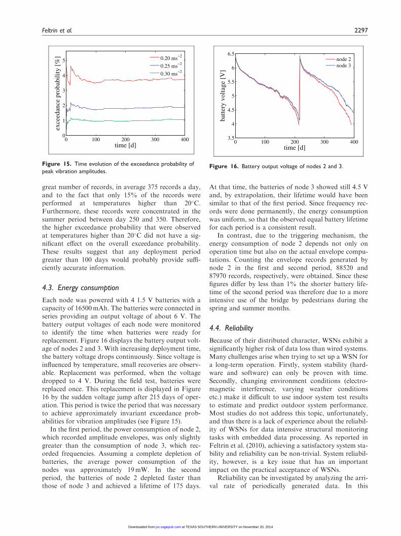
great number of records, in average 375 records a day,and to the fact that only 15% of the records wereperformed at temperatures higher than 20�C.Furthermore, these records were concentrated in thesummer period between day 250 and 350. Therefore,the higher exceedance probability that were observedat temperatures higher than 20�C did not have a sig-nificant effect on the overall exceedance probability.These results suggest that any deployment periodgreater than 100 days would probably provide suffi-ciently accurate information.

4.3. Energy consumption

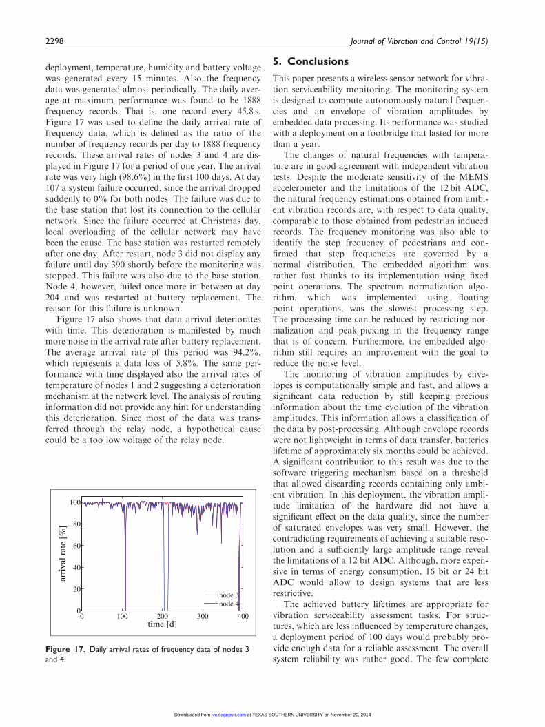
Each node was powered with 4 1.5 V batteries with acapacity of 16500mAh. The batteries were connected inseries providing an output voltage of about 6 V. Thebattery output voltages of each node were monitoredto identify the time when batteries were ready forreplacement. Figure 16 displays the battery output volt-age of nodes 2 and 3. With increasing deployment time,the battery voltage drops continuously. Since voltage isinfluenced by temperature, small recoveries are observ-able. Replacement was performed, when the voltagedropped to 4 V. During the field test, batteries werereplaced once. This replacement is displayed in Figure16 by the sudden voltage jump after 215 days of oper-ation. This period is twice the period that was necessaryto achieve approximately invariant exceedance prob-abilities for vibration amplitudes (see Figure 15).

In the first period, the power consumption of node 2,which recorded amplitude envelopes, was only slightlygreater than the consumption of node 3, which rec-orded frequencies. Assuming a complete depletion ofbatteries, the average power consumption of thenodes was approximately 19mW. In the secondperiod, the batteries of node 2 depleted faster thanthose of node 3 and achieved a lifetime of 175 days.

At that time, the batteries of node 3 showed still 4.5 Vand, by extrapolation, their lifetime would have beensimilar to that of the first period. Since frequency rec-ords were done permanently, the energy consumptionwas uniform, so that the observed equal battery lifetimefor each period is a consistent result.

In contrast, due to the triggering mechanism, theenergy consumption of node 2 depends not only onoperation time but also on the actual envelope compu-tations. Counting the envelope records generated bynode 2 in the first and second period, 88520 and87970 records, respectively, were obtained. Since thesefigures differ by less than 1% the shorter battery life-time of the second period was therefore due to a moreintensive use of the bridge by pedestrians during thespring and summer months.

4.4. Reliability

Because of their distributed character, WSNs exhibit asignificantly higher risk of data loss than wired systems.Many challenges arise when trying to set up a WSN fora long-term operation. Firstly, system stability (hard-ware and software) can only be proven with time.Secondly, changing environment conditions (electro-magnetic interference, varying weather conditionsetc.) make it difficult to use indoor system test resultsto estimate and predict outdoor system performance.Most studies do not address this topic, unfortunately,and thus there is a lack of experience about the reliabil-ity of WSNs for data intensive structural monitoringtasks with embedded data processing. As reported inFeltrin et al. (2010), achieving a satisfactory system sta-bility and reliability can be non-trivial. System reliabil-ity, however, is a key issue that has an importantimpact on the practical acceptance of WSNs.

Reliability can be investigated by analyzing the arri-val rate of periodically generated data. In this

0 100 200 300 4000

1

2

3

4

5ex

ceed

ance

pro

babi

lity

[%]

time [d]

0.20 ms−2

0.25 ms−2

0.30 ms−2

Figure 15. Time evolution of the exceedance probability of

peak vibration amplitudes.

0 100 200 300 4003.5

4

4.5

5

5.5

6

6.5

time [d]

batte

ry v

olta

ge [

V]

node 2node 3

Figure 16. Battery output voltage of nodes 2 and 3.

Feltrin et al. 2297



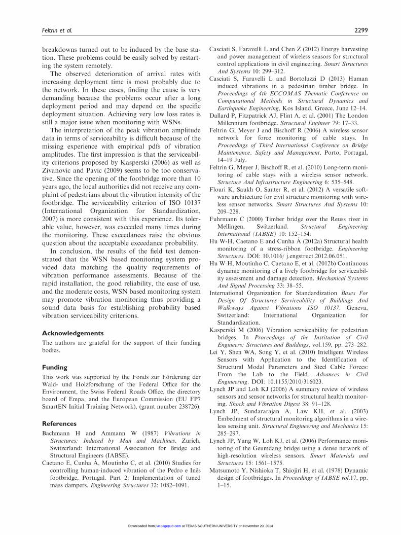
deployment, temperature, humidity and battery voltagewas generated every 15 minutes. Also the frequencydata was generated almost periodically. The daily aver-age at maximum performance was found to be 1888frequency records. That is, one record every 45.8 s.Figure 17 was used to define the daily arrival rate offrequency data, which is defined as the ratio of thenumber of frequency records per day to 1888 frequencyrecords. These arrival rates of nodes 3 and 4 are dis-played in Figure 17 for a period of one year. The arrivalrate was very high (98.6%) in the first 100 days. At day107 a system failure occurred, since the arrival droppedsuddenly to 0% for both nodes. The failure was due tothe base station that lost its connection to the cellularnetwork. Since the failure occurred at Christmas day,local overloading of the cellular network may havebeen the cause. The base station was restarted remotelyafter one day. After restart, node 3 did not display anyfailure until day 390 shortly before the monitoring wasstopped. This failure was also due to the base station.Node 4, however, failed once more in between at day204 and was restarted at battery replacement. Thereason for this failure is unknown.

Figure 17 also shows that data arrival deteriorateswith time. This deterioration is manifested by muchmore noise in the arrival rate after battery replacement.The average arrival rate of this period was 94.2%,which represents a data loss of 5.8%. The same per-formance with time displayed also the arrival rates oftemperature of nodes 1 and 2 suggesting a deteriorationmechanism at the network level. The analysis of routinginformation did not provide any hint for understandingthis deterioration. Since most of the data was trans-ferred through the relay node, a hypothetical causecould be a too low voltage of the relay node.

5. Conclusions

This paper presents a wireless sensor network for vibra-tion serviceability monitoring. The monitoring systemis designed to compute autonomously natural frequen-cies and an envelope of vibration amplitudes byembedded data processing. Its performance was studiedwith a deployment on a footbridge that lasted for morethan a year.

The changes of natural frequencies with tempera-ture are in good agreement with independent vibrationtests. Despite the moderate sensitivity of the MEMSaccelerometer and the limitations of the 12 bit ADC,the natural frequency estimations obtained from ambi-ent vibration records are, with respect to data quality,comparable to those obtained from pedestrian inducedrecords. The frequency monitoring was also able toidentify the step frequency of pedestrians and con-firmed that step frequencies are governed by anormal distribution. The embedded algorithm wasrather fast thanks to its implementation using fixedpoint operations. The spectrum normalization algo-rithm, which was implemented using floatingpoint operations, was the slowest processing step.The processing time can be reduced by restricting nor-malization and peak-picking in the frequency rangethat is of concern. Furthermore, the embedded algo-rithm still requires an improvement with the goal toreduce the noise level.

The monitoring of vibration amplitudes by enve-lopes is computationally simple and fast, and allows asignificant data reduction by still keeping preciousinformation about the time evolution of the vibrationamplitudes. This information allows a classification ofthe data by post-processing. Although envelope recordswere not lightweight in terms of data transfer, batterieslifetime of approximately six months could be achieved.A significant contribution to this result was due to thesoftware triggering mechanism based on a thresholdthat allowed discarding records containing only ambi-ent vibration. In this deployment, the vibration ampli-tude limitation of the hardware did not have asignificant effect on the data quality, since the numberof saturated envelopes was very small. However, thecontradicting requirements of achieving a suitable reso-lution and a sufficiently large amplitude range revealthe limitations of a 12 bit ADC. Although, more expen-sive in terms of energy consumption, 16 bit or 24 bitADC would allow to design systems that are lessrestrictive.

The achieved battery lifetimes are appropriate forvibration serviceability assessment tasks. For struc-tures, which are less influenced by temperature changes,a deployment period of 100 days would probably pro-vide enough data for a reliable assessment. The overallsystem reliability was rather good. The few complete

0 100 200 300 4000

20

40

60

80

100

time [d]

arri

val r

ate

[%]

node 3node 4

Figure 17. Daily arrival rates of frequency data of nodes 3

and 4.




breakdowns turned out to be induced by the base sta-tion. These problems could be easily solved by restart-ing the system remotely.

The observed deterioration of arrival rates withincreasing deployment time is most probably due tothe network. In these cases, finding the cause is verydemanding because the problems occur after a longdeployment period and may depend on the specificdeployment situation. Achieving very low loss rates isstill a major issue when monitoring with WSNs.

The interpretation of the peak vibration amplitudedata in terms of serviceability is difficult because of themissing experience with empirical pdfs of vibrationamplitudes. The first impression is that the serviceabil-ity criterions proposed by Kasperski (2006) as well asZivanovic and Pavic (2009) seems to be too conserva-tive. Since the opening of the footbridge more than 10years ago, the local authorities did not receive any com-plaint of pedestrians about the vibration intensity of thefootbridge. The serviceability criterion of ISO 10137(International Organization for Standardization,2007) is more consistent with this experience. Its toler-able value, however, was exceeded many times duringthe monitoring. These exceedances raise the obviousquestion about the acceptable exceedance probability.

In conclusion, the results of the field test demon-strated that the WSN based monitoring system pro-vided data matching the quality requirements ofvibration performance assessments. Because of therapid installation, the good reliability, the ease of use,and the moderate costs, WSN based monitoring systemmay promote vibration monitoring thus providing asound data basis for establishing probability basedvibration serviceability criterions.

Acknowledgements

The authors are grateful for the support of their funding

bodies.

Funding

This work was supported by the Fonds zur Forderung derWald- und Holzforschung of the Federal Office for theEnvironment, the Swiss Federal Roads Office, the directory

board of Empa, and the European Commission (EU FP7SmartEN Initial Training Network), (grant number 238726).

References

Bachmann H and Ammann W (1987) Vibrations in

Structures: Induced by Man and Machines. Zurich,

Switzerland: International Association for Bridge and

Structural Engineers (IABSE).Caetano E, Cunha A, Moutinho C, et al. (2010) Studies for

controlling human-induced vibration of the Pedro e Ines

footbridge, Portugal. Part 2: Implementation of tuned

mass dampers. Engineering Structures 32: 1082–1091.

Casciati S, Faravelli L and Chen Z (2012) Energy harvestingand power management of wireless sensors for structuralcontrol applications in civil engineering. Smart Structures

And Systems 10: 299–312.Casciati S, Faravelli L and Bortoluzzi D (2013) Human

induced vibrations in a pedestrian timber bridge. InProceedings of 4th ECCOMAS Thematic Conference on

Computational Methods in Structural Dynamics andEarthquake Engineering, Kos Island, Greece, June 12–14.

Dallard P, Fitzpatrick AJ, Flint A, et al. (2001) The London

Millennium footbridge. Structural Engineer 79: 17–33.Feltrin G, Meyer J and Bischoff R (2006) A wireless sensor

network for force monitoring of cable stays. In

Proceedings of Third International Conference on BridgeMaintenance, Safety and Management, Porto, Portugal,14–19 July.

Feltrin G, Meyer J, Bischoff R, et al. (2010) Long-term moni-toring of cable stays with a wireless sensor network.Structure And Infrastructure Engineering 6: 535–548.

Flouri K, Saukh O, Sauter R, et al. (2012) A versatile soft-

ware architecture for civil structure monitoring with wire-less sensor networks. Smart Structures And Systems 10:209–228.

Fuhrmann C (2000) Timber bridge over the Reuss river inMellingen, Switzerland. Structural EngineeringInternational (IABSE) 10: 152–154.

Hu W-H, Caetano E and Cunha A (2012a) Structural healthmonitoring of a stress-ribbon footbridge. EngineeringStructures. DOI: 10.1016/ j.engstruct.2012.06.051.

Hu W-H, Moutinho C, Caetano E, et al. (2012b) Continuous

dynamic monitoring of a lively footbridge for serviceabil-ity assessment and damage detection. Mechanical SystemsAnd Signal Processing 33: 38–55.

International Organization for Standardization Bases ForDesign Of Structures - Serviceability of Buildings AndWalkways Against Vibrations ISO 10137. Geneva,

Switzerland: International Organization forStandardization.

Kasperski M (2006) Vibration serviceability for pedestrian

bridges. In Proceedings of the Institution of CivilEngineers: Structures and Buildings, vol.159, pp. 273–282.

Lei Y, Shen WA, Song Y, et al. (2010) Intelligent WirelessSensors with Application to the Identification of

Structural Modal Parameters and Steel Cable Forces:From the Lab to the Field. Advances in CivilEngineering. DOI: 10.1155/2010/316023.

Lynch JP and Loh KJ (2006) A summary review of wirelesssensors and sensor networks for structural health monitor-ing. Shock and Vibration Digest 38: 91–128.

Lynch JP, Sundararajan A, Law KH, et al. (2003)Embedment of structural monitoring algorithms in a wire-less sensing unit. Structural Engineering and Mechanics 15:285–297.

Lynch JP, Yang W, Loh KJ, et al. (2006) Performance moni-toring of the Geumdang bridge using a dense network ofhigh-resolution wireless sensors. Smart Materials and

Structures 15: 1561–1575.Matsumoto Y, Nishioka T, Shiojiri H, et al. (1978) Dynamic

design of footbridges. In Proceedings of IABSE vol.17, pp.

1–15.

Feltrin et al. 2299



Racic V, Pavic A and Brownjohn JMW (2009) Experimentalidentification and analytical modelling of human walkingforces: Literature review. Journal of Sound and Vibration

326: 1–49.Zimmerman AT, Shiraishi M, Swartz RA, et al. (2008)

Automated modal parameter estimation by parallel pro-cessing within wireless monitoring systems. Journal of

Infrastructure Systems 14: 102–113.Zivanovic S (2012) Benchmark footbridge for vibration ser-

viceability assessment under the vertical component of

pedestrian load. Journal of Structural Engineering 138:1193–1202.

Zivanovic S and Pavic A (2009) Probabilistic assessment of

human response to footbridge vibration. Journal of LowFrequency Noise, Vibration and Active Control 28:255–268.

Zivanovic S, Pavic A and Reynolds P (2005) Vibration

serviceability of footbridges under human-induced excita-tion: a literature review. Journal of Sound and Vibration279: 1–74.




Documents

Vibration monitoring of a footbridge with a wireless sensor network