Vibration fatigue analysis of components on rotating ... Vibration fatigue... · The output from a Rainflow cycle counting exercise is expressed as a 'Rainflow histogram' showing

SoSDiD 2017 May 17-18, 2017 Darmstadt, Germany

VIBRATION FATIGUE ANALYSIS OF COMPONENTS ON ROTATING

MACHINERY UNDER SINE AND SWEPT-SINE-ON-RANDOM LOADING

A Halfpenny, F Kihm, R Plaskitt,

HBM-Prenscia, Technology Centre, Brunel Way, Rotherham S60 5WG, UK

ABSTRACT

This paper describes an approach for calculating the high-cycle fatigue life of a component

subjected to sine-on-random loading. The calculation method is based on a spectral

approach in the frequency-domain. This offers significant advantages over the time-domain

approach when finite element analysis calculation times become prohibitive. A statistical

Rainflow cycle histogram is derived directly from a sine-on-random spectrum of stress. The

cycles are applied to an appropriate material fatigue curve in order to obtain the estimated

life. A case study is presented to illustrate the method using a component attached to a

helicopter. Comparisons with traditional time-domain approaches are presented and show

excellent agreement. The paper concludes by showing how this method was extended to

cover the case of swept-sine-on-random excitation.

KEYWORDS

Sine-on-Random, Swept-Sine-on-Random, Random Vibration, Vibration, Frequency-

domain, Power Spectral Density (PSD), Finite Element Analysis (FEA), Rainflow Cycle

Count, Fatigue Analysis.

INTRODUCTION

Sine-on-random excitations are typically generated by rotating machinery. The term ‘sine-

on-random’ implies a series of sinusoidal tones, usually harmonics of the rotation speed,

superimposed on a background of random noise. Pure sine-on-random excitations are seen

during constant-speed rotation, while swept-sine-on-random excitations are seen during

variable-speed rotation.

Long-term exposure of equipment to vibration gives rise to microscopic cracks that

eventually propagate to failure; a failure mode referred to as ‘Fatigue’. Equipment is tested

and qualified against fatigue failure to standards such as MIL-STD-810G [1], Def Stan 00-

35 [2] and RTCA/DO160G [3]. So far, the only way of estimating fatigue life from a sine-

on-random excitation is to perform a transient finite element analysis in the time-domain.

The time signal is constructed by superimposing sinusoidal harmonics on a time-domain

realization of the random PSD (Power Spectral Density function). Such analyses are often

accelerated by using modal superposition but are still very demanding in terms of CPU

time. It also raises the question of how long the excitation signal should be in order to

ensure convergence on fatigue life. The time-domain approach is therefore impractical and

this is the main reason why a spectral approach is relevant.


Spectral methods of estimating fatigue damage in the frequency-domain are well

established. Bendat [4] published a report showing how the Rayleigh distribution could be

used to estimate the fatigue cycles in a narrow-band random process. Steinberg [5]

demonstrated how the Gaussian-normal distribution could be used in the case of a broad-

band process. Dirlik [6] and Bishop [7] describe the derivation of an empirical probability

distribution that is suitable over a range of bandwidths. And Lalanne [8] provides an

analytical probability distribution based on Rice's [9] distribution of peaks in a random

signal. All these methods are summarised by Halfpenny and Kihm [10] along with a

comparison study of these methods with reference to the time-domain process of 'Rainflow'

cycle counting.

A limitation with all these spectral methods is that they require the underlying time signal

of stress to be 'Stochastic'. This implies that its amplitude statistics are 'Stationary, Ergodic

and Gaussian Random'. In practice this means that the 'phase' content of the random signal

is also random and can consist of any phase angle with equal probability. This assumption

is necessary for many reasons, not least because the loads are often expressed in the form of

a PSD.

A PSD contains information on the amplitude and frequency content of a signal, but it does

not contain information on the 'phase' content. By definition a sinusoidal signal is

'Deterministic' and not 'Stochastic'. It has a finite 'phase' angle and its amplitude is not

random. Although it is possible to calculate the PSD of a sine-on-random signal, this PSD

alone does not offer a complete representation of the signal. This is because the phase

content is missing and it cannot be approximated by a random value. Any attempt to

calculate the fatigue cycles based on a Stochastic assumption is likely to underestimate the

actual damage. This is because the sinusoidal tones present in the PSD representation

would be interpreted as narrow-band random processes. In this case, the narrow-band

processes would share the same RMS (Root Mean Square) amplitude as the sinusoidal

tones but would not have the same peak amplitude. The purpose of this paper is to derive a

new probability distribution in order to determine the fatigue cycles present in a sine-on-

random signal.

METHODOLOGY

This section describes an approach for computing the fatigue life, or damage, of a

component subjected to sine-on-random loading. The loading definition is expressed as a

PSD of the random background signal along with a table of the sinusoidal frequencies and

their amplitudes. The derivation starts with a brief summary of fatigue estimation in the

time-domain before continuing to the new spectral approach. It concludes with a discussion

on how this method may be extended further to consider the case of swept-sine-on-random

loading.


Review of stress-life (SN) fatigue analysis in the time-domain

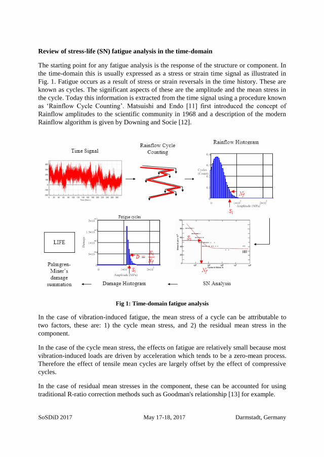
The starting point for any fatigue analysis is the response of the structure or component. In

the time-domain this is usually expressed as a stress or strain time signal as illustrated in

Fig. 1. Fatigue occurs as a result of stress or strain reversals in the time history. These are

known as cycles. The significant aspects of these are the amplitude and the mean stress in

the cycle. Today this information is extracted from the time signal using a procedure known

as ‘Rainflow Cycle Counting’. Matsuishi and Endo [11] first introduced the concept of

Rainflow amplitudes to the scientific community in 1968 and a description of the modern

Rainflow algorithm is given by Downing and Socie [12].

Fig 1: Time-domain fatigue analysis

In the case of vibration-induced fatigue, the mean stress of a cycle can be attributable to

two factors, these are: 1) the cycle mean stress, and 2) the residual mean stress in the

component.

In the case of the cycle mean stress, the effects on fatigue are relatively small because most

vibration-induced loads are driven by acceleration which tends to be a zero-mean process.

Therefore the effect of tensile mean cycles are largely offset by the effect of compressive

cycles.

In the case of residual mean stresses in the component, these can be accounted for using

traditional R-ratio correction methods such as Goodman's relationship [13] for example.


The output from a Rainflow cycle counting exercise is expressed as a 'Rainflow histogram'

showing the number of cycles vs. the stress amplitude. Each cycle will induce a certain

amount of fatigue damage on the component and this is quantified with a fatigue curve

similar to the SN curve illustrated. The total damage over the entire test is obtained by

summing the damage in each bin of the Rainflow histogram. This approach is known as the

'Palmgren-Miner accumulated damage rule', [14][15].

The damage caused by each cycle is calculated with reference to the material life curve, in

this case the SN curve. The SN curve shows the number of cycles to failure, 𝑁𝑓, for a given

stress amplitude, 𝑆. The total damage caused by 𝑁 number of cycles is therefore obtained

as the ratio of cycles present in the time signal to the number of cycles to failure. The

Palmgren-Miner rule can therefore be expressed as equation 1.

𝐷 =∑𝑁𝑖𝑁𝑓

𝑖

(1)

𝐷 is the fatigue damage ratio. If 𝐷 ≥ 1 then the component is likely to fail within the

duration of the test. If 𝐷 < 1 then the fatigue life is determined as 𝑇/𝐷 seconds, where 𝑇 is

the duration of the test in seconds. 𝑁𝑖 is the number of cycles in the 𝑖𝑡ℎ bin in the histogram

with stress amplitude 𝑆𝑖, and 𝑁𝑓 is the number of cycles to failure for that particular stress

amplitude.

In this example the fatigue life curve is represented in terms of a SN (or Wöhler) curve.

This is often presented as a series of piecewise linear segments in log-space where each

segment is represented as equation 2.

𝐶 = 𝑁𝑓𝑆𝑏

(2)

𝑆 is the stress amplitude in 𝑀𝑃𝑎, 𝑁𝑓 is the number of Rainflow cycles to failure, 𝐶 is the

Basquin coefficient (intercept of the SN curve with the Stress axis) and 𝑏 is the Basquin

exponent (gradient of the SN curve in log space). The fatigue damage ratio is therefore

obtained by substituting equation 2 into equation 1 as given in equation 3.

𝐷 =1

𝐶∑𝑁𝑖𝑖

𝑆𝑖𝑏

(3)

where 𝑆𝑖 is the stress amplitude of the 𝑖𝑡ℎ fatigue cycle in the time signal.


New spectral SN fatigue method

Spectral fatigue proceeds in a manner similar to the time-domain except that the Rainflow

cycle counting algorithm is replaced with one based on a Probability Density Function

(PDF) of stress amplitude; for example, the Rayleigh, Dirlik or Lalanne PDFs. The end

result of the PDF methods is shown as a Rainflow histogram and equation 3 is replaced

with equation 4.

𝐷 =𝐸𝑝𝑇

𝐶∫ 𝑝∞

0

(𝑆) 𝑆𝑏𝑑𝑆

(4)

𝑝(𝑆) is the PDF of fatigue cycles, 𝐸𝑝 is the expected number of fatigue cycles per second of

test exposure and 𝑇 is the test exposure time in seconds.

Using moments of area under the PSD, Rice [9] derived formulae to estimate the number of

peaks per second, 𝐸𝑝, as well as the number of zero up-crossings per second 𝐸0. These are

given in equation 5.

𝐸0 = √𝑚2

𝑚0

𝐸𝑝 = √𝑚4

𝑚2

(5)

𝑚0, 𝑚2 and 𝑚4 are the 0𝑡ℎ, 2𝑛𝑑 and 4𝑡ℎ moments of the PSD about the zero 𝐻𝑧 axis. The

𝑛𝑡ℎ moment of area is defined by equation 6. (Note: 𝑚0 is equal to the area under the PSD

which also represents the 'mean square' value of the time signal or the square of the RMS)

𝑚𝑛 = ∫ 𝑓𝑛∞

0

𝐺(𝑓)𝑑𝑓

(6)

𝐺(𝑓) is the single sided PSD of stress amplitude at frequency 𝑓𝐻𝑧.

A reliable measure of bandwidth was also offered by Rice [9] as a ratio of the number of

zero up-crossings in a time signal to the number of peaks. This ratio is often known as the

'irregularity factor 𝛾' and is given by equation 7. For narrow-band signals the irregularity

factor tends to one (all peaks occur above the mean) whereas for white noise it tends to √5

9.


𝛾 =𝐸0𝐸𝑝

=𝑚2

√𝑚0𝑚4

(7)

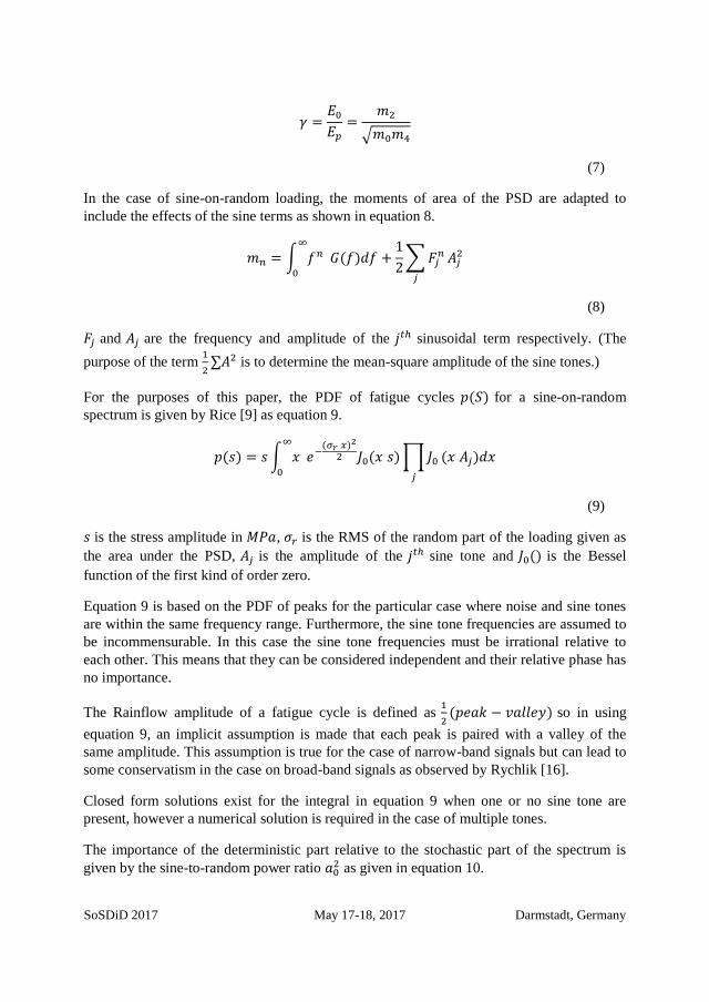
In the case of sine-on-random loading, the moments of area of the PSD are adapted to

include the effects of the sine terms as shown in equation 8.

𝑚𝑛 = ∫ 𝑓𝑛∞

0

𝐺(𝑓)𝑑𝑓 +1

2∑𝐹𝑗

𝑛

𝑗

𝐴𝑗2

(8)

𝐹𝑗 and 𝐴𝑗 are the frequency and amplitude of the 𝑗𝑡ℎ sinusoidal term respectively. (The

purpose of the term 1

2∑𝐴2 is to determine the mean-square amplitude of the sine tones.)

For the purposes of this paper, the PDF of fatigue cycles 𝑝(𝑆) for a sine-on-random

spectrum is given by Rice [9] as equation 9.

𝑝(𝑠) = 𝑠∫ 𝑥∞

0

𝑒−(𝜎𝑟 𝑥)2

2 𝐽0(𝑥 𝑠)∏𝐽0𝑗

(𝑥 𝐴𝑗)𝑑𝑥

(9)

𝑠 is the stress amplitude in 𝑀𝑃𝑎, 𝜎𝑟 is the RMS of the random part of the loading given as

the area under the PSD, 𝐴𝑗 is the amplitude of the 𝑗𝑡ℎ sine tone and 𝐽0() is the Bessel

function of the first kind of order zero.

Equation 9 is based on the PDF of peaks for the particular case where noise and sine tones

are within the same frequency range. Furthermore, the sine tone frequencies are assumed to

be incommensurable. In this case the sine tone frequencies must be irrational relative to

each other. This means that they can be considered independent and their relative phase has

no importance.

The Rainflow amplitude of a fatigue cycle is defined as 1

2(𝑝𝑒𝑎𝑘 − 𝑣𝑎𝑙𝑙𝑒𝑦) so in using

equation 9, an implicit assumption is made that each peak is paired with a valley of the

same amplitude. This assumption is true for the case of narrow-band signals but can lead to

some conservatism in the case on broad-band signals as observed by Rychlik [16].

Closed form solutions exist for the integral in equation 9 when one or no sine tone are

present, however a numerical solution is required in the case of multiple tones.

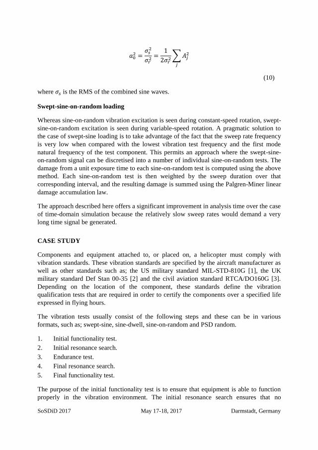
The importance of the deterministic part relative to the stochastic part of the spectrum is

given by the sine-to-random power ratio 𝑎02 as given in equation 10.


𝑎02 =

𝜎𝑠2

𝜎𝑟2=

1

2𝜎𝑟2∑𝐴𝑗

2

𝑗

(10)

where 𝜎𝑠 is the RMS of the combined sine waves.

Swept-sine-on-random loading

Whereas sine-on-random vibration excitation is seen during constant-speed rotation, swept-

sine-on-random excitation is seen during variable-speed rotation. A pragmatic solution to

the case of swept-sine loading is to take advantage of the fact that the sweep rate frequency

is very low when compared with the lowest vibration test frequency and the first mode

natural frequency of the test component. This permits an approach where the swept-sine-

on-random signal can be discretised into a number of individual sine-on-random tests. The

damage from a unit exposure time to each sine-on-random test is computed using the above

method. Each sine-on-random test is then weighted by the sweep duration over that

corresponding interval, and the resulting damage is summed using the Palgren-Miner linear

damage accumulation law.

The approach described here offers a significant improvement in analysis time over the case

of time-domain simulation because the relatively slow sweep rates would demand a very

long time signal be generated.

CASE STUDY

Components and equipment attached to, or placed on, a helicopter must comply with

vibration standards. These vibration standards are specified by the aircraft manufacturer as

well as other standards such as; the US military standard MIL-STD-810G [1], the UK

military standard Def Stan 00-35 [2] and the civil aviation standard RTCA/DO160G [3].

Depending on the location of the component, these standards define the vibration

qualification tests that are required in order to certify the components over a specified life

expressed in flying hours.

The vibration tests usually consist of the following steps and these can be in various

formats, such as; swept-sine, sine-dwell, sine-on-random and PSD random.

1. Initial functionality test.

2. Initial resonance search.

3. Endurance test.

4. Final resonance search.

5. Final functionality test.

The purpose of the initial functionality test is to ensure that equipment is able to function

properly in the vibration environment. The initial resonance search ensures that no


significant structural mode is excited by a principal vibration frequency of the aircraft, for

example, a harmonic of the blade rotor frequency. The endurance test exposes the

equipment to an entire life-time's worth of vibration damage over a highly accelerated time

frame. The final resonance search ensure that no changes are apparent in the resonant

response of the equipment that could be indicative of a progressive structural failure. And

the final functionality test ensures that the equipment is still fully functional following the

test. Vibration testing can be expensive and it is therefore useful to simulate the test

computationally in order to avoid foreseeable problems.

This case study considers an item of equipment mounted externally on a helicopter. The

equipment failed under the specified endurance test. The failure was thought to be due to a

vibration mode occurring close to the blade-passing frequency of the helicopter. The

equipment supplier therefore wanted advice on the failure mechanism in order to redesign

the equipment to achieve the required qualification.

In order to determine if the equipment failed due to fatigue cracking, the vibration test was

simulated using nCode DesignLife with MSC Nastran. Two analysis techniques were used.

The first considered a frequency-domain simulation using Nastran SOL 111, (modal

frequency response), along with the spectral fatigue method described in this paper. The

second considered a time-domain simulation using Nastran SOL 112, (modal transient

response), along with a time signal reconstruction of the sine-on-random test profile.

Excitation spectrum

The sine-on-random excitation spectrum was derived using MIL-STD-810G. A comparison

with service flight loads showed an under-estimate in some ranges of the spectrum and so

test tailoring was performed as described by Halfpenny and Walton [17]. The sine-on-

random spectrum is illustrated in Fig. 2. A random profile is used between 10 and 500Hz

with sine tones applied at harmonics of the blade passing frequency (1nR, 2nR and 3nR).

The vertical and lateral accelerations were found to dominate the loading environment,

whereas the fore/aft axis is relatively benign. Only the vertical axis is considered in this

paper.

Fig. 2: Sine-on-random excitation spectrum


Stress response

Both a transient dynamic analysis and a frequency response analysis were performed using

MSC Nastran. The transient dynamic analysis produces a time series of stress, whereas a

frequency response analysis produces a complex frequency response matrix in the modal

coordinate system. nCode DesignLife was used to process these data. The analysis

consisted of modal summation followed by a multiaxial critical plane fatigue analysis.

Using this technique, stresses at each node are resolved on to a rotating axis frame and the

axis with the most critical damage is reported. Modal summation was performed in

DesignLife in order to reduce the size of data transferred between the two software

packages. For the purposes of time-domain simulation, a test signal of 100 seconds was

produced at a sample rate of 1024 points per second. A typical time signal of stress

response is shown in Fig. 3.

Fig. 3: Typical time signal representation of stress response at node

Fig. 4 shows typical spectral results for two nodes on the model. Fig. 4a illustrates the case

of a narrow-banded response excited principally by the random component of the signal,

whereas, Fig 4b illustrates the case of a broad-banded response excited significantly by a

harmonic of the blade passing frequency. The characteristics of the two responses are

summarised in Table 1.

Table 1: Characteristics of the two responses.

Location Sine to power ratio 𝑎02 Irregularity factor 𝛾

a 1.2 0.98

b 8.2 0.87


Fig. 4: Sine-on-random stress response spectrum at two locations, a and b, on the component.

Rainflow cycle distributions and fatigue life estimation

Fig. 5 compares the rainflow cycle histogram obtained from the time-domain solution (red)

with that obtained using the spectral approach (blue) for both critical locations on the

model.

Fig. 5: Comparison between rainflow cycles using the time-domain (red) and spectral (blue)

approaches.

With reference to Table 1, location a: we observe from the irregularity factor, 𝛾 = 0.98,

that the stress response at this location is relatively narrow-banded and from the sine to

power ratio, 𝑎02 = 1.2, that the influence of the sine tones is approximately the same as the

random noise. From Fig. 4a, the response could be described as a single mode response that

is excited by the random vibration portion of the sine-on-random signal. With exception of

the lowest frequency sine tone, which is of relatively low amplitude, the dominant sine

tones lie within the frequency range of the random noise. Furthermore, the sine tone


frequencies are associated with harmonics of the blade passing frequency and so occur at

multiples of each other. Therefore location a does not respect strictly the assumptions made

in the derivation described in this paper. However, the derived stress PDF shown in Fig. 5a

still shows excellent correlation with the rainflow histogram obtained through rainflow

cycle counting in the time-domain. The time-domain simulation used here was limited to a

duration of 100 seconds because of the high computational effort. It is likely that this has

curtailed some of the high amplitude cycles, seen at the right of the histogram, that would

otherwise have occurred in a longer signal.

With reference to Table 1, location b: we observe from the irregularity factor, 𝛾 = 0.87,

that the stress response at this location is relatively broad-banded and from the sine to

power ratio, 𝑎02 = 8.2, that the influence of the sine tones is dominant. From Fig. 4b, the

response could be described as a multi-modal response where the second structural mode is

excited by the second sinusoidal harmonic. This situation will highlight further the effect of

the assumptions made in the method's derivation. However, the resulting stress PDF shown

in Fig. 5b still shows excellent correlation with the rainflow histogram obtained through

rainflow cycle counting in the time-domain. The sparsely populated rainflow bins at the

right of the histogram again highlight the limitations of the time signal duration on properly

resolving the higher amplitude cycles.

Table 2 compares the fatigue damage ratio estimates obtained at the two critical locations

using both the time-domain and spectral methods.

Table 2: Fatigue damage ratio estimates.

Location

Fatigue damage from time-

domain

Fatigue damage from frequency-

domain Discrepancy

a 16E-3 23E-3 44%

b 26E-3 36E-3 38%

The fatigue damage estimates given in Table 2 show excellent correlation between the two

methods. The discrepancy of approximately 40%, which is small in terms of fatigue, shows

that the time-domain approach is underestimating the damage when compared with the

spectral approach. This is explained because of the sparsely populated rainflow bins

towards the right-hand side of the rainflow histogram. If the time signal reconstruction were

made much longer, then more cycles would be observed at the extreme ranges thereby

increasing the fatigue damage. In this case the spectral approach is considered more

representative and reliable than the time-domain.

The final fatigue life estimates were found to be within a factor of 2 of the number of hours

of testing to cause the crack. Under these circumstances, such an accurate result is

acknowledged to be somewhat down to chance.


CONCLUSION

A spectral approach to fatigue analysis offers advantages over the time-domain approach

when limited stress time history data are available or computation times are prohibitive. A

very robust method of deriving fatigue estimates for sine-on-random vibration is presented

and a method for extending this to also consider swept-sine-on-random is also discussed.

A case study is presented that compares fatigue analysis using the spectral approach with

that of the time-domain approach for a component attached to the fuselage of a helicopter.

Excellent correlation between the two approaches is demonstrated. In this case study, the

results from the spectral approach are found to be more reliable than those from the time-

domain approach. This is because the spectral approach is able to implicitly account for the

statistically rare occurrence of high amplitude cycles that only appear over long duration

exposure. These cycles are missing from the time signal reconstruction because of the

relatively short exposure simulated.

The approach offers an efficient means for ‘virtual vibration testing’ based on FEA

simulation. The benefits of numerical simulation include:

• Pre-test validation – virtual testing can highlight design problems before committing

to physical component testing.

• Test optimisation – ensures that the test specification delivers the desired damage in

the least amount of time.

• Ensure that the test is not ‘over-accelerated’, i.e. the sine-on-random amplitude is not

excessively severe which could give rise to local plasticity and a change in the failure

mode.

• Estimate the residual life, safety margin and confidence levels of a component where

physical tests do not run to destruction or where the number of physical tests are

limited.

• Estimate the effect of amplitude ‘clipping’ in the physical test, for example, clipping

applied at ±3𝜎 amplitude.

Before now, the approach for high-cycle fatigue damage assessment under random

vibration was limited to Gaussian random loads. The new method extends this to consider

the non-Gaussian case where multiple sine tones are superimposed on the Gaussian random

loads. This new method is particularly useful for fatigue analysis of components subjected

to vibration generated by rotating machinery.


REFERENCES

[1] 2008, MIL-Std-810g: Test Method Standard for Environmental Engineering

Considerations and Laboratory Tests, United States Department of Defense.

[2] Def Stan 00-35: Environmental Handbook for Defence Materiel, Part 3: Environmental

Test Methods., UK Ministry of Defence.

[3] 2010, RCA/Do-160 Revision G: Environmental Conditions and Test Procedures for

Airborne Equipment, RTCA.

[4] Bendat, J., 1964, Probability Functions for Random Responses, NASA report on

contract NAS-5-4590.

[5] Steinberg, D., 2000, Vibration Analysis for Electronic Equipment, Wiley-Interscience.

[6] Dirlik, T., 1985, “Application of Computers in Fatigue Analysis,” PhD thesis,

University of Warwick, UK.

[7] Bishop, N., and Sherratt, F., 1989, “Fatigue Life Prediction from Power Spectral

Density Data,” Environmental Engineering, 2.

[8] Lalanne, C., 2009, Mechanical Vibration and Shock Analysis, Fatigue Damage, Wiley.

[9] Rice, S., 1944, “Mathematical Analysis of Random Noise,” Bell System Technical

Journal, 23, pp. 282–332.

[10] Halfpenny, A., and Kihm, F., 2010, “Rainflow Cycle Counting and Acoustic Fatigue

Analysis Techniques for Random Loading.”

[11] Matsuishi, M., and Endo, T., 1968, “Fatigue of Metals Subjected to Varying Stress.”

[12] Downing, S., and Socie, D., 1982, “Simple Rainflow Counting Algorithms,” Int. J.

Fatigue, 4(1), pp. 31–40.

[13] Goodman, J., 1899, Mechanics Applied to Engineering, Longman, Green & Company,

London.

[14] Palmgren, A., 1924, “Die Lebensdauer von Kugellagern (the Service Life of

Bearings),” Zeitschrift des vereinesdeutscher ingenierure (Magazine of the Association of

German Engineers), 68(14), pp. 339–341.

[15] Miner, M., 1945, “Cumulative Damage in Fatigue,” J. Appl. Mech., 67, pp. A159–

A164.

[16] Rychlik, I., 1993, “On the ‘Narrow-Band’ Approximation for Expected Fatigue

Damage,” Probab. Eng. Mech., 8, pp. 1–4.

[17] Halfpenny, A., and Walton, T., 2010, “New Techniques for Vibration Qualification of

Vibrating Equipment on Aircraft.”

Corresponding author: [email protected]

Documents

Vibration fatigue analysis of components on rotating ... Vibration fatigue... · The output from a Rainflow cycle counting exercise is expressed as a 'Rainflow histogram' showing