Embed Size (px)
Citation preview
Contents1 Overview 3
2 Computation and Annotation 52.1 Computing Venn drawings . . . . . . . . . . . . . . . . . . . . . . . 52.2 Annotation parameters . . . . . . . . . . . . . . . . . . . . . . . . . 62.3 Graphical parameters . . . . . . . . . . . . . . . . . . . . . . . . . . 7
3 Unweighted Venn diagrams 103.1 Unweighted 2-set Venn diagrams . . . . . . . . . . . . . . . . . . . . 103.2 Unweighted 3-set Venn diagrams . . . . . . . . . . . . . . . . . . . . 113.3 Unweighted 4-set Venn diagrams . . . . . . . . . . . . . . . . . . . . 123.4 Unweighted Venn diagrams on more than four sets . . . . . . . . . . 14
4 Weighted Venn diagrams 164.1 Weighted 2-set Venn diagrams for 2 Sets . . . . . . . . . . . . . . . . 16
4.1.1 Circles . . . . . . . . . . . . . . . . . . . . . . . . . . . . . 164.1.2 Squares . . . . . . . . . . . . . . . . . . . . . . . . . . . . . 16
4.2 Weighted 3-set Venn diagrams . . . . . . . . . . . . . . . . . . . . . 184.2.1 Circles . . . . . . . . . . . . . . . . . . . . . . . . . . . . . 184.2.2 Squares . . . . . . . . . . . . . . . . . . . . . . . . . . . . . 194.2.3 Triangles . . . . . . . . . . . . . . . . . . . . . . . . . . . . 21
4.3 Chow-Ruskey diagrams for 3 or more sets . . . . . . . . . . . . . . . 22
5 Euler diagrams 255.1 2-set Euler diagrams . . . . . . . . . . . . . . . . . . . . . . . . . . 25
5.1.1 Circles . . . . . . . . . . . . . . . . . . . . . . . . . . . . . 255.1.2 Squares . . . . . . . . . . . . . . . . . . . . . . . . . . . . . 26
5.2 3-set Euler diagrams . . . . . . . . . . . . . . . . . . . . . . . . . . 285.2.1 Circles . . . . . . . . . . . . . . . . . . . . . . . . . . . . . 285.2.2 Triangles . . . . . . . . . . . . . . . . . . . . . . . . . . . . 30
5.3 4-set Euler diagrams . . . . . . . . . . . . . . . . . . . . . . . . . . 325.3.1 Chow-Ruskey diagrams . . . . . . . . . . . . . . . . . . . . 32
6 Some loose definitions 33
7 This document 34
2

1 OverviewThe Vennerable package provides routines to compute and plot Venn diagrams, includ-ing the classic two- and three-circle diagrams but also a variety of others with differentproperties and for up to seven sets. In addition it can plot diagrams in which the area ofeach region is proportional to the corresponding number of set items or other weights.This includes Euler diagrams, which can be thought of as Venn diagrams where regionscorresponding to empty intersections have been removed.
Figure 1 shows a three-circle Venn diagram of the sort commonly found. To drawit, we use as an example the StemCell data of Boyer et al.[? ] which lists the genenames associated with each of four transcription factors
> library(Vennerable)
> data(StemCell)
> str(StemCell)
List of 4
$ OCT4 : chr [1:623] "AASDH" "ABTB2" "ACCN4" "ACD" ...
$ SOX2 : chr [1:1279] "182-FIP" "AASDH" "ABCA5" "ABCB10" ...
$ NANOG: chr [1:1687] "13CDNA73" "AASDH" "ABCA5" "ABCB10" ...
$ E2F4 : chr [1:1273] "76P" "7h3" "AAMP" "AATF" ...
First we construct an object of class Venn:
> Vstem <- Venn(StemCell)
> Vstem
A Venn object on 4 sets named
OCT4,SOX2,NANOG,E2F4
0000 1000 0100 1100 0010 1010 0110 1110 0001 1001 0101 1101 0011 1011 0111 1111
0 109 305 45 644 64 354 287 821 30 78 6 118 16 138 66
Although Vennerable can cope with 4-set Venn diagrams, for now we reduce to a three-set object
> Vstem3 <- Vstem[, c("OCT4", "SOX2", "NANOG")]
> Vstem3
A Venn object on 3 sets named
OCT4,SOX2,NANOG
000 100 010 110 001 101 011 111
821 139 383 51 762 80 492 353
Note how the weights were appropriately updated.Now a call to plot produces the diagram in Figure 1 showing how many genes are
common to each transcription factor.
3
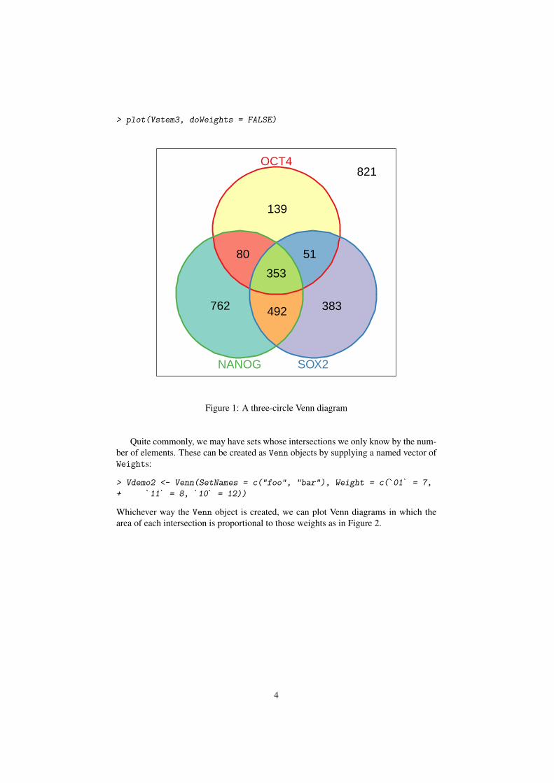
> plot(Vstem3, doWeights = FALSE)
OCT4
SOX2NANOG
762 383492
139
80 51
353
821
Figure 1: A three-circle Venn diagram
Quite commonly, we may have sets whose intersections we only know by the num-ber of elements. These can be created as Venn objects by supplying a named vector ofWeights:
> Vdemo2 <- Venn(SetNames = c("foo", "bar"), Weight = c(`01` = 7,
+ `11` = 8, `10` = 12))
Whichever way the Venn object is created, we can plot Venn diagrams in which thearea of each intersection is proportional to those weights as in Figure 2.
4
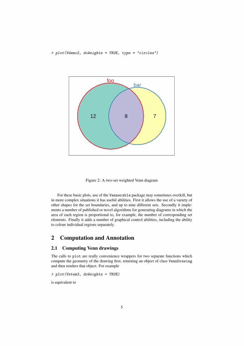
> plot(Vdemo2, doWeights = TRUE, type = "circles")
foobar
712 8
Figure 2: A two-set weighted Venn diagram
For these basic plots, use of the Vennerable package may sometimes overkill, butin more complex situations it has useful abilities. First it allows the use of a variety ofother shapes for the set boundaries, and up to nine different sets. Secondly it imple-ments a number of published or novel algorithms for generating diagrams in which thearea of each region is proportional to, for example, the number of corresponding setelements. Finally it adds a number of graphical control abilities, including the abilityto colour individual regions separately.
2 Computation and Annotation
2.1 Computing Venn drawingsThe calls to plot are really convenience wrappers for two separate functions whichcompute the geometry of the drawing first, returning an object of class VennDrawingand then renders that object. For example
> plot(Vstem3, doWeights = TRUE)
is equivalent to
5
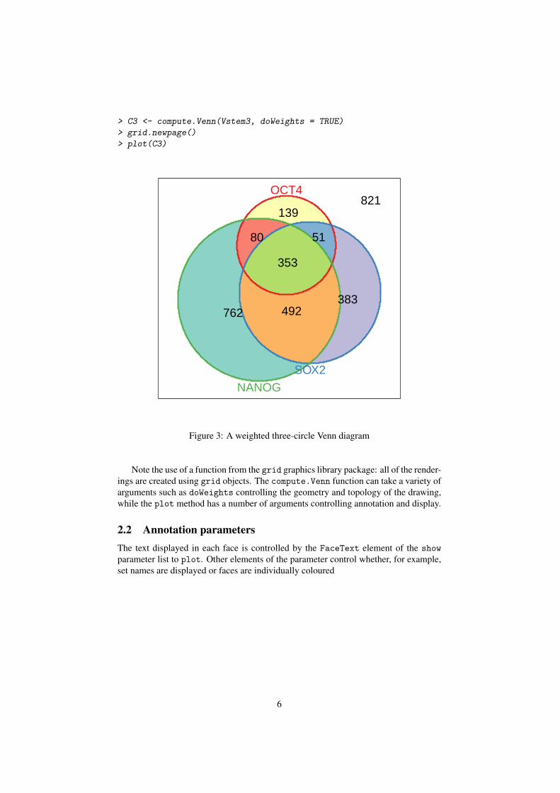
> C3 <- compute.Venn(Vstem3, doWeights = TRUE)
> grid.newpage()
> plot(C3)
OCT4
SOX2
NANOG
762383
492
139
80 51
353
821
Figure 3: A weighted three-circle Venn diagram
Note the use of a function from the grid graphics library package: all of the render-ings are created using grid objects. The compute.Venn function can take a variety ofarguments such as doWeights controlling the geometry and topology of the drawing,while the plot method has a number of arguments controlling annotation and display.
2.2 Annotation parametersThe text displayed in each face is controlled by the FaceText element of the show
parameter list to plot. Other elements of the parameter control whether, for example,set names are displayed or faces are individually coloured
6
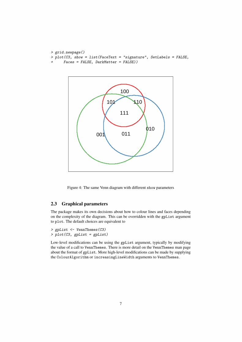
> grid.newpage()
> plot(C3, show = list(FaceText = "signature", SetLabels = FALSE,
+ Faces = FALSE, DarkMatter = FALSE))
001010
011
100
101 110
111
Figure 4: The same Venn diagram with different show parameters
2.3 Graphical parametersThe package makes its own decisions about how to colour lines and faces dependingon the complexity of the diagram. This can be overridden with the gpList argumentto plot. The default choices are equivalent to
> gpList <- VennThemes(C3)
> plot(C3, gpList = gpList)
Low-level modifications can be using the gpList argument, typically by modifyingthe value of a call to VennThemes. There is more detail on the VennThemes man pageabout the format of gpList. More high-level modifications can be made by supplyingthe ColourAlgorithm or increasingLineWidth arguments to VennThemes.
7

> grid.newpage()
> gp <- VennThemes(C3, colourAlgorithm = "binary")
> plot(C3, gpList = gp, show = list(FaceText = "sets", SetLabels = FALSE,
+ Faces = TRUE))
32
23
1
13 12
123
Figure 5: The effect of setting ColourAlgorithm="binary" and FaceText="sets"
The position and format of the set and face annotation are controlled by the data re-turned by VennGetSetLabels and VennGetFaceLabels, respectively, which can bemodified and then reembedded in the VennDrawing object with VennSetSetLabels
and VennSetFaceLabels.
8

> grid.newpage()
> SetLabels <- VennGetSetLabels(C3)
> SetLabels[SetLabels$Label == "February", "y"] <- SetLabels[SetLabels$Label ==
+ "March", "y"]
> C3 <- VennSetSetLabels(C3, SetLabels)
> plot(C3)
OCT4
SOX2
NANOG
762383
492
139
80 51
353
821
Figure 6: Modifying the position of annotation
9
3 Unweighted Venn diagramsFor another running example, we use sets named after months, whose elements are theletters of their names.
> setList <- strsplit(month.name, split = "")
> names(setList) <- month.name
> Vmonth3 <- VennFromSets(setList[1:3])
> Vmonth2 <- Vmonth3[, c("January", "February"), ]
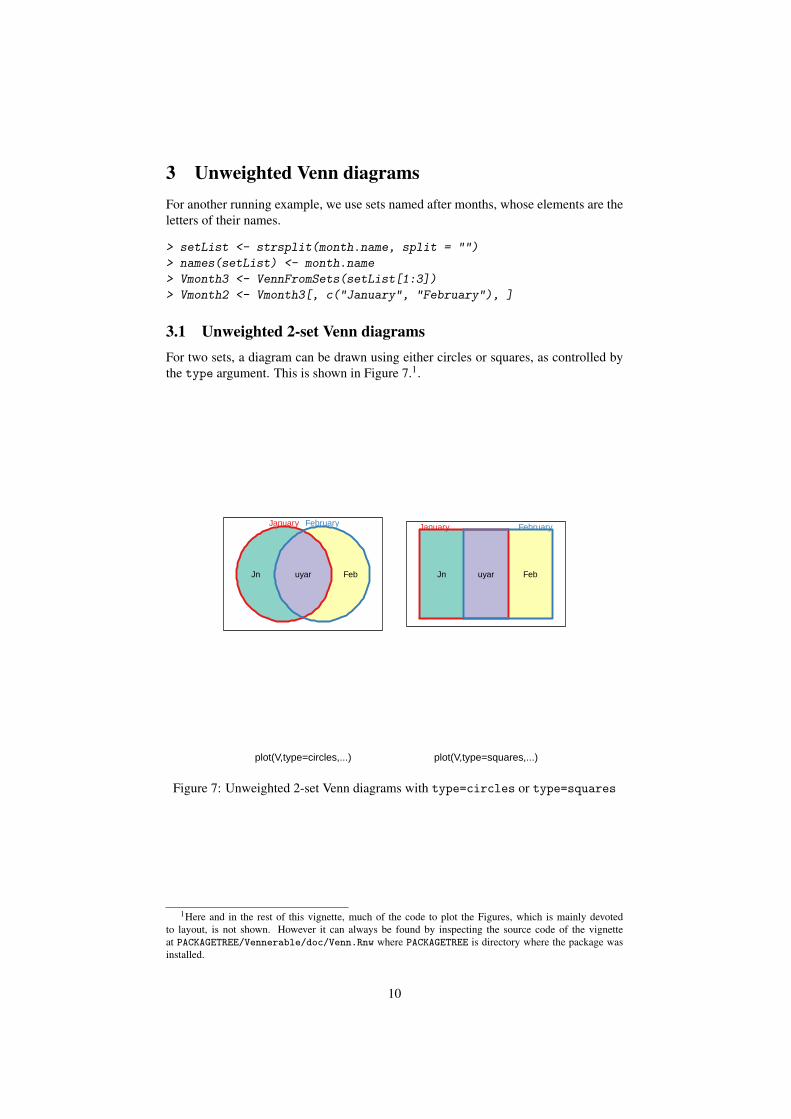
3.1 Unweighted 2-set Venn diagramsFor two sets, a diagram can be drawn using either circles or squares, as controlled bythe type argument. This is shown in Figure 7.1.
plot(V,type=circles,...)
January February
FebJn uyar
plot(V,type=squares,...)
January February
FebJn uyar
Figure 7: Unweighted 2-set Venn diagrams with type=circles or type=squares
1Here and in the rest of this vignette, much of the code to plot the Figures, which is mainly devotedto layout, is not shown. However it can always be found by inspecting the source code of the vignetteat PACKAGETREE/Vennerable/doc/Venn.Rnw where PACKAGETREE is directory where the package wasinstalled.
10
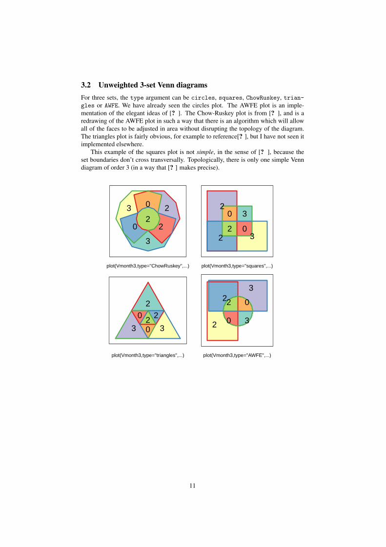
3.2 Unweighted 3-set Venn diagramsFor three sets, the type argument can be circles, squares, ChowRuskey, trian-gles or AWFE. We have already seen the circles plot. The AWFE plot is an imple-mentation of the elegant ideas of [? ]. The Chow-Ruskey plot is from [? ], and is aredrawing of the AWFE plot in such a way that there is an algorithm which will allowall of the faces to be adjusted in area without disrupting the topology of the diagram.The triangles plot is fairly obvious, for example to reference[? ], but I have not seen itimplemented elsewhere.
This example of the squares plot is not simple, in the sense of [? ], because theset boundaries don’t cross transversally. Topologically, there is only one simple Venndiagram of order 3 (in a way that [? ] makes precise).
plot(Vmonth3,type="ChowRuskey",...)
3
3
0
20
22
plot(Vmonth3,type="squares",...)
3
30
20
22
plot(Vmonth3,type="triangles",...)
3 30
20 22
plot(Vmonth3,type="AWFE",...)
3
3
0
2 0
22
11
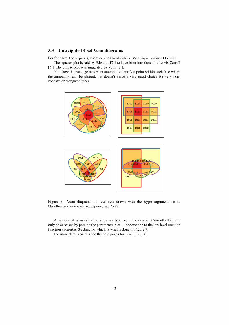
3.3 Unweighted 4-set Venn diagramsFor four sets, the type argument can be ChowRuskey, AWFE,squares or ellipses.
The squares plot is said by Edwards [? ] to have been introduced by Lewis Carroll[? ]. The ellipse plot was suggested by Venn [? ].
Note how the package makes an attempt to identify a point within each face wherethe annotation can be plotted, but doesn’t make a very good choice for very non-concave or elongated faces.
0001
0010
0011
01000101
0110
0111
1000
10011010
1011
1100
1101
1110
1111
0001
0010
0011
0100
0101
0110
0111
1000
1001
1010
1011
1100
1101
1110
1111
0001 0010
0011
0100
0101
0110
0111 1000
1001
1010
1011
110011011110
1111 00010010
0011
01000101
01100111
1000
10011010
1011
11001101
11101111
Figure 8: Venn diagrams on four sets drawn with the type argument set toChowRuskey, squares, ellipses, and AWFE.
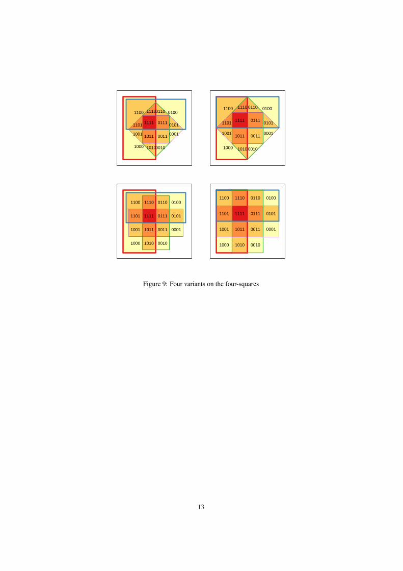
A number of variants on the squares type are implemented. Currently they canonly be accessed by passing the parameters s or likesquares to the low level creationfunction compute.S4 directly, which is what is done in Figure 9.
For more details on this see the help pages for compute.S4.
12
0001
0010
0011
0100
0101
0110
0111
1000
1001
1010
1011
1100
1101
1110
1111
0001
0010
0011
0100
0101
0110
0111
1000
1001
1010
1011
1100
1101
1110
1111
0001
0010
0011
0100
0101
0110
0111
1000
1001
1010
1011
1100
1101
1110
1111
0001
0010
0011
0100
0101
0110
0111
1000
1001
1010
1011
1100
1101
1110
1111
Figure 9: Four variants on the four-squares
13
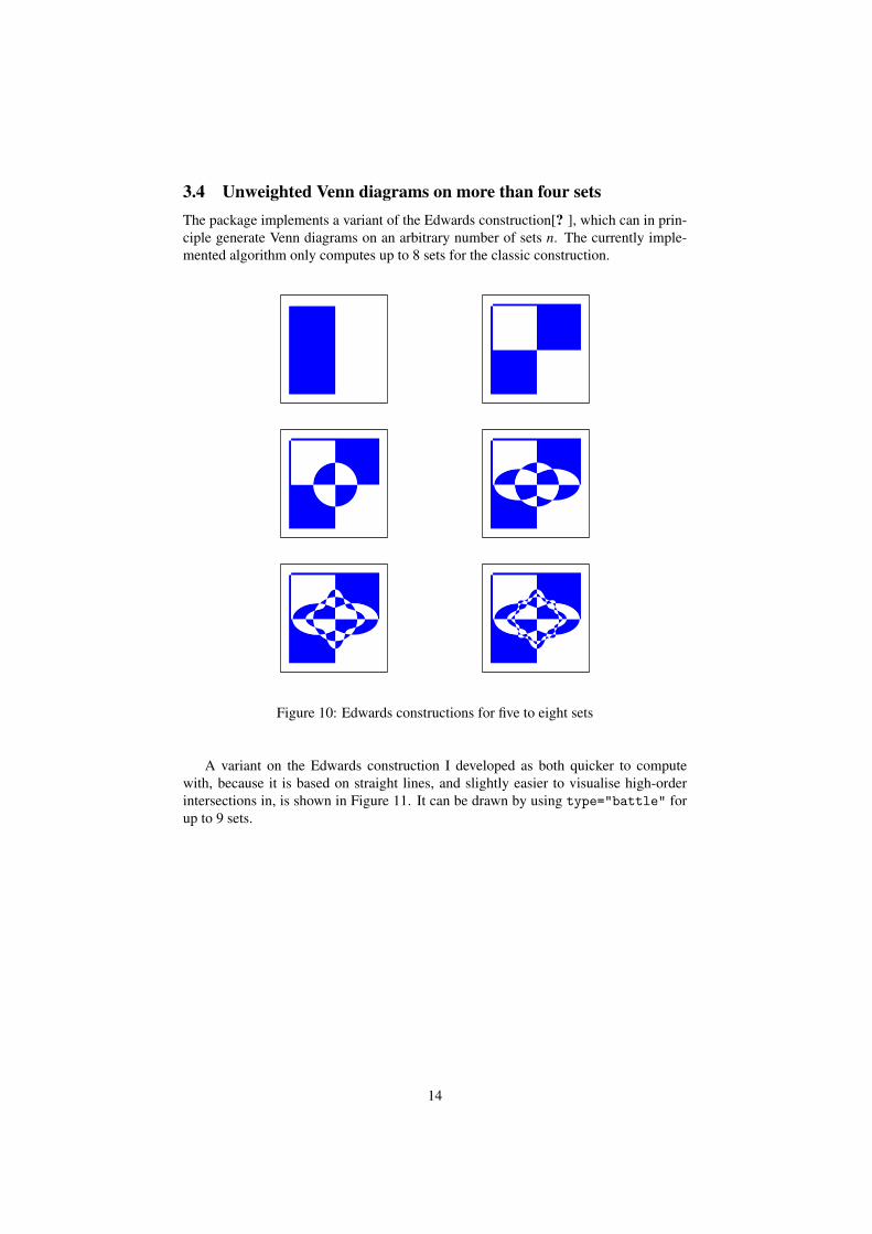
3.4 Unweighted Venn diagrams on more than four setsThe package implements a variant of the Edwards construction[? ], which can in prin-ciple generate Venn diagrams on an arbitrary number of sets n. The currently imple-mented algorithm only computes up to 8 sets for the classic construction.
Figure 10: Edwards constructions for five to eight sets
A variant on the Edwards construction I developed as both quicker to computewith, because it is based on straight lines, and slightly easier to visualise high-orderintersections in, is shown in Figure 11. It can be drawn by using type="battle" forup to 9 sets.
14
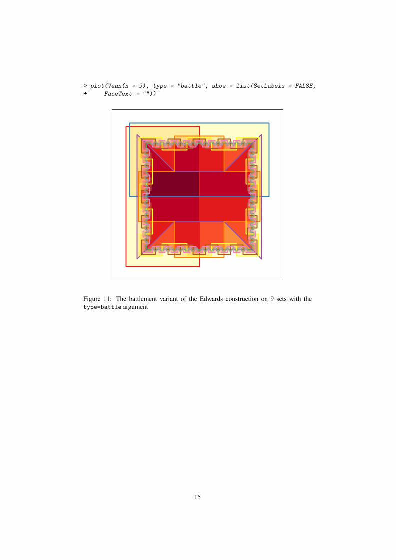
> plot(Venn(n = 9), type = "battle", show = list(SetLabels = FALSE,
+ FaceText = ""))
Figure 11: The battlement variant of the Edwards construction on 9 sets with thetype=battle argument
15

4 Weighted Venn diagramsThere are repeated requests to generate Venn diagrams in which the areas of the facesthemselves are meant to carry information, mainly by being proportional to the in-tersection weights. Even when these diagrams can be drawn, they are not often asuccess in their information-bearing mission. But we can try anyway, through use ofthe argument doWeights=TRUE. First of all we consider the case when all the visibleintersection weights are nonzero.
4.1 Weighted 2-set Venn diagrams for 2 Sets4.1.1 Circles
It is always possible to get an exactly area-weighted solution for two circles as shownin Figure 12.
> V3.big <- Venn(SetNames = LETTERS[1:3], Weight = 2^(1:8))
> Vmonth2.big <- V3.big[, c(1:2)]
> plot(Vmonth2.big)
AB
13668 272
34
Figure 12: Weighted 2d Venn
4.1.2 Squares
As for circles, square weight-proportional diagrams can be simply constructed.
16

> plot(Vmonth2.big, type = "squares")
AB136
68 272
34
Figure 13: Weighted 2d Venn squares
17
4.2 Weighted 3-set Venn diagrams4.2.1 Circles
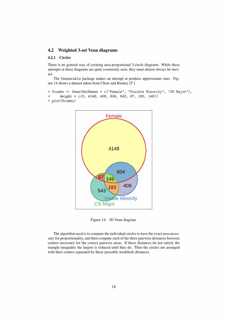
There is no general way of creating area-proportional 3-circle diagrams. While theseattempts at these diagrams are quite commonly seen, they must almost always be inex-act.
The Vennerable package makes an attempt at produce approximate ones. Fig-ure 14 shows a dataset taken from Chow and Ruskey [? ]
> Vcombo <- Venn(SetNames = c("Female", "Visible Minority", "CS Major"),
+ Weight = c(0, 4148, 409, 604, 543, 67, 183, 146))
> plot(Vcombo)
Female
Visible MinorityCS Major
543409183
4148
67604
146
Figure 14: 3D Venn diagram
The algorithm used is to compute the individual circles to have the exact area neces-sary for proportionality, and then compute each of the three pairwise distances betweencentres necessary for the correct pairwise areas. If these distances do not satisfy thetriangle inequality the largest is reduced until they do. Then the circles are arrangedwith their centres separated by these (possibly modified) distances.
18
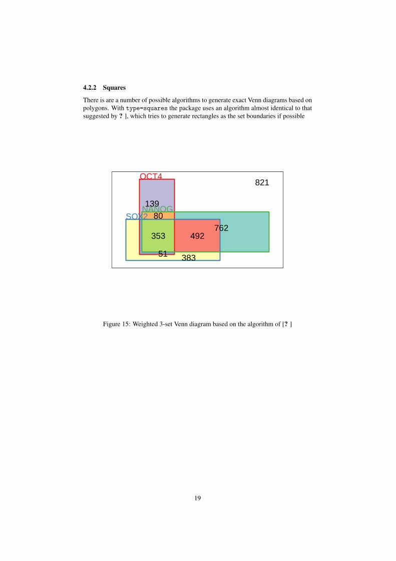
4.2.2 Squares
There is are a number of possible algorithms to generate exact Venn diagrams based onpolygons. With type=squares the package uses an algorithm almost identical to thatsuggested by ? ], which tries to generate rectangles as the set boundaries if possible
OCT4
SOX2NANOG
762
383
492
13980
51
353
821
Figure 15: Weighted 3-set Venn diagram based on the algorithm of [? ]
19
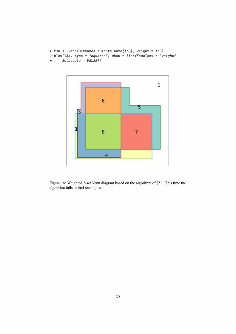
> V3a <- Venn(SetNames = month.name[1:3], Weight = 1:8)
> plot(V3a, type = "squares", show = list(FaceText = "weight",
+ SetLabels = FALSE))
5
3 7
2
6
4
8
1
Figure 16: Weighted 3-set Venn diagram based on the algorithm of [? ]. This time thealgorithm fails to find rectangles.
20

4.2.3 Triangles
The triangular Venn diagram on 3-sets lends itself nicely to an area-proportional draw-ing under some contraints on the weights (detailed elsewhere).
> grid.newpage()
> C3t <- compute.Venn(V3a, type = "triangles")
> plot(C3t, show = list(SetLabels = FALSE, DarkMatter = FALSE))
5
3
7
2
6
4
8
Figure 17: Weighted Triangular Venn diagram
21
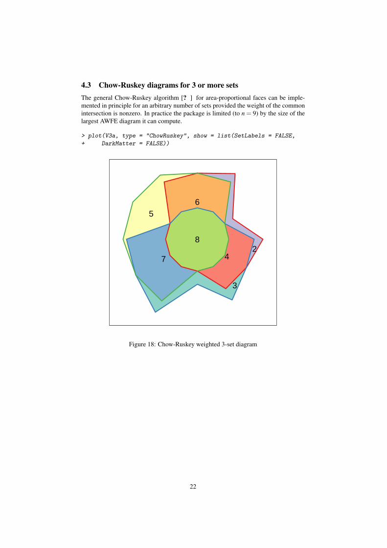
4.3 Chow-Ruskey diagrams for 3 or more setsThe general Chow-Ruskey algorithm [? ] for area-proportional faces can be imple-mented in principle for an arbitrary number of sets provided the weight of the commonintersection is nonzero. In practice the package is limited (to n = 9) by the size of thelargest AWFE diagram it can compute.
> plot(V3a, type = "ChowRuskey", show = list(SetLabels = FALSE,
+ DarkMatter = FALSE))
5
3
72
6
4
8
Figure 18: Chow-Ruskey weighted 3-set diagram
22

> V4a <- Venn(SetNames = LETTERS[1:4], Weight = 16:1)
> plot(V4a, type = "ChowRuskey", show = list(SetLabels = FALSE,
+ DarkMatter = FALSE))
8
12
4
14
6
10
2
15
7
11
3
13
5
9
1
Figure 19: Chow-Ruskey weighted 4-set diagram
23
OCT4
SOX2
NANOG
E2F4
821
644
118
305
78
354
138
10930
64
16
45
6
287
66
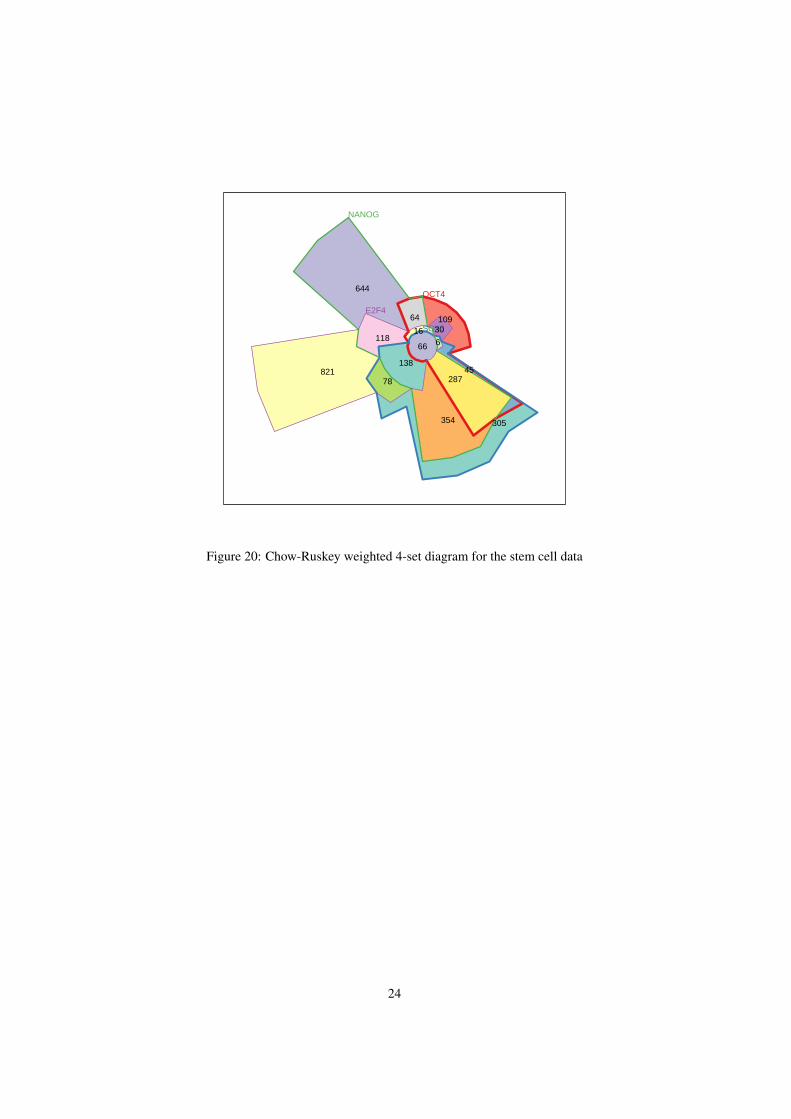
Figure 20: Chow-Ruskey weighted 4-set diagram for the stem cell data
24
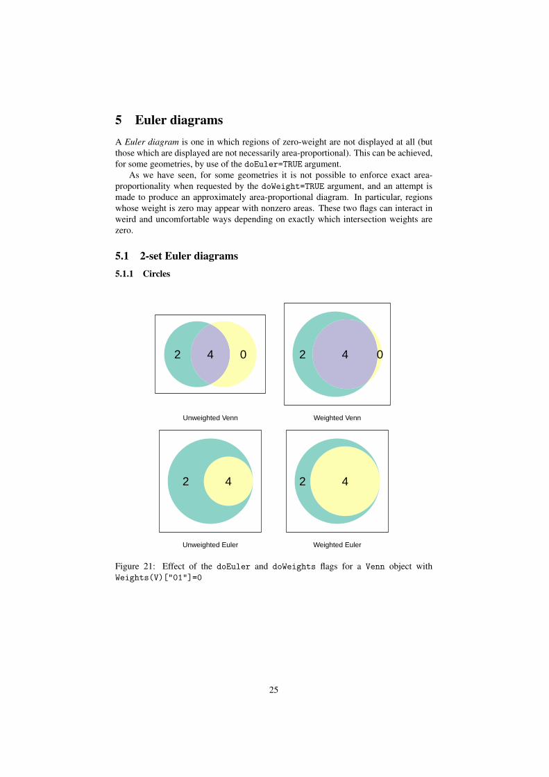
5 Euler diagramsA Euler diagram is one in which regions of zero-weight are not displayed at all (butthose which are displayed are not necessarily area-proportional). This can be achieved,for some geometries, by use of the doEuler=TRUE argument.
As we have seen, for some geometries it is not possible to enforce exact area-proportionality when requested by the doWeight=TRUE argument, and an attempt ismade to produce an approximately area-proportional diagram. In particular, regionswhose weight is zero may appear with nonzero areas. These two flags can interact inweird and uncomfortable ways depending on exactly which intersection weights arezero.
5.1 2-set Euler diagrams5.1.1 Circles
Unweighted Venn
02 4
Weighted Venn
02 4
Unweighted Euler
2 4
Weighted Euler
2 4
Figure 21: Effect of the doEuler and doWeights flags for a Venn object withWeights(V)["01"]=0
25
Unweighted Venn
32 0
Weighted Venn
32 0
Unweighted Euler
32
Weighted Euler
32
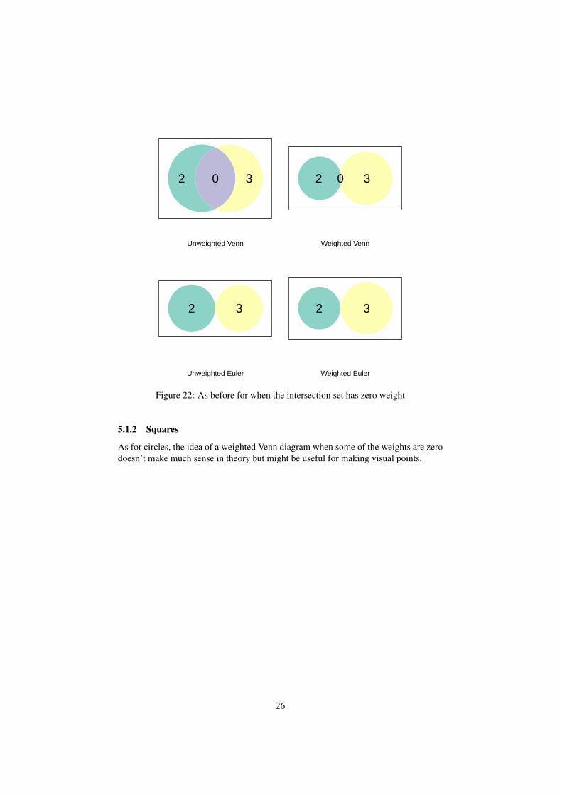
Figure 22: As before for when the intersection set has zero weight
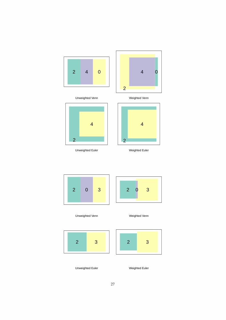
5.1.2 Squares
As for circles, the idea of a weighted Venn diagram when some of the weights are zerodoesn’t make much sense in theory but might be useful for making visual points.
26
Unweighted Venn
02 4
Weighted Venn
0
2
4
Unweighted Euler
2
4
Weighted Euler
2
4
Unweighted Venn
32 0
Weighted Venn
32 0
Unweighted Euler
32
Weighted Euler
32
27

5.2 3-set Euler diagrams5.2.1 Circles
There is currently no effect of setting doEuler=TRUE for three circles, but the doWeights=TRUEflag does an approximate job. There are about 40 distinct ways in which intersectionregions can have zeroes can occur, but here are some examples.
April
May
July
Ju
May
Apri
l
April
MayNovember
Novemb May
Apilr
April
MayJune
June May
April
September
MayJune
JunMay
Sptmbr
e
Figure 23: Weighted 3d Venn empty intersections.
28
January
FebruaryMarch
MchFeb
Jn
uy
ar
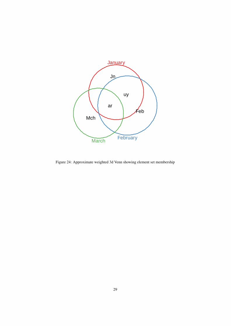
Figure 24: Approximate weighted 3d Venn showing element set membership
29
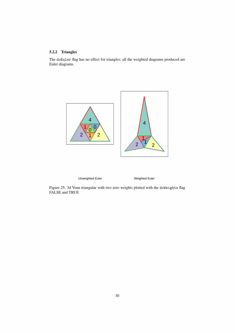
5.2.2 Triangles
The doEuler flag has no effect for triangles; all the weighted diagrams produced areEuler diagrams.
Unweighted Euler
2 21
41 00
Weighted Euler
2 21
4
1
Figure 25: 3d Venn triangular with two zero weights plotted with the doWeights flagFALSE and TRUE
30
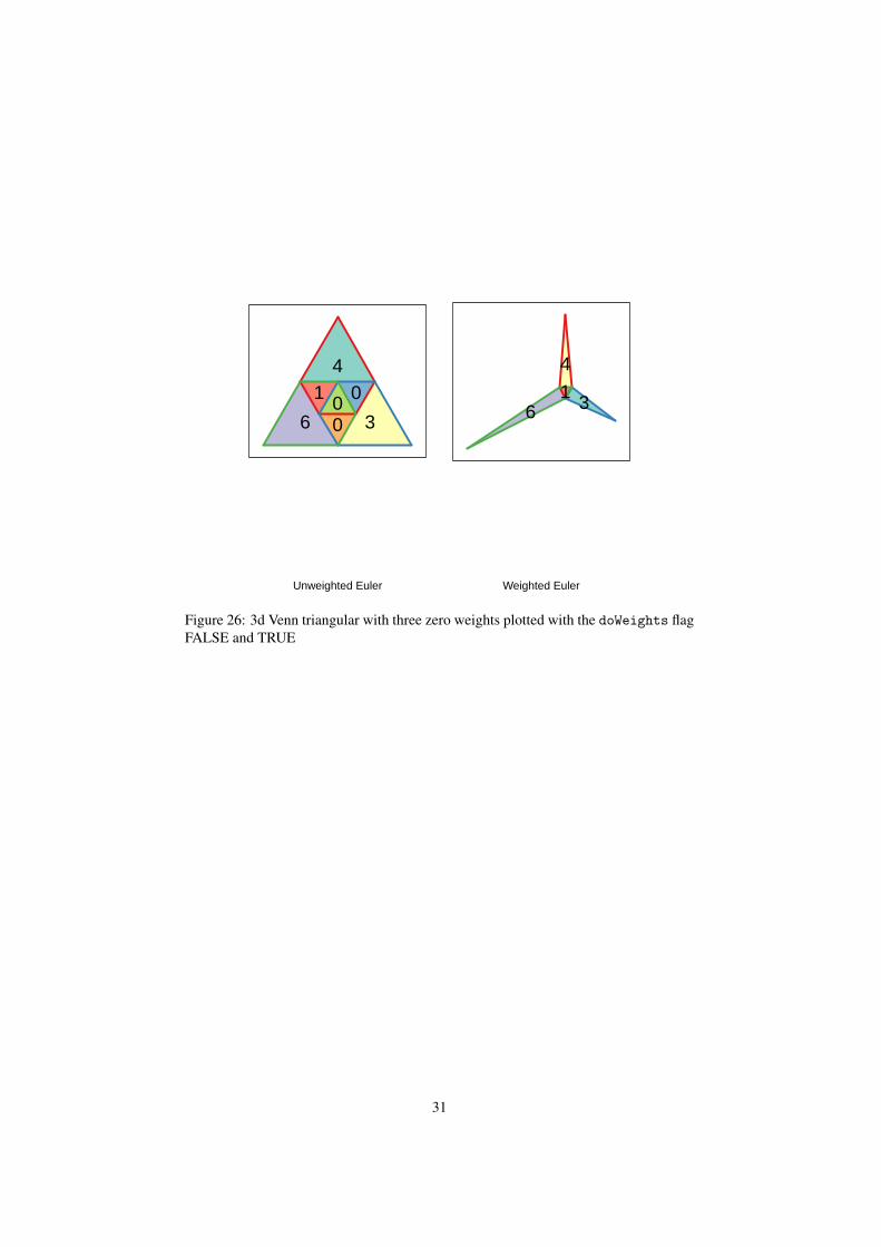
Unweighted Euler
6 30
41 00
Weighted Euler
6 3
4
1
Figure 26: 3d Venn triangular with three zero weights plotted with the doWeights flagFALSE and TRUE
31

5.3 4-set Euler diagrams5.3.1 Chow-Ruskey diagrams
The doEuler flag has no effect for Chow-Ruskey because all the weighted diagramsproduced are already Euler diagrams.
Apil
Mch
Feb
Jn
uya
r
Figure 27: Chow-Ruskey diagram with some zero weights
32
6 Some loose definitionsFigure 1 illustrates membership of three sets, in order OCT4, SOX2 , NANOG. Geneswhich are members of the SOX2 set but not the OCT4 or NANOG sets are membersof an intersection subset with indicator string or signature 010.
Given n sets of elements drawn from a universe, there are 2n intersection subsets.Each of these is a subset of the universe and there is one corresponding to each of thebinary strings of length n. If one of these indicator strings has a 1 in the i-th position,all of members of the corresponding intersection subset must be members of the i-thset. Depending on the application, the universe of elements from which members ofthe sets are drawn may be important. Elements in intersection set 00..., which are inthe universe but not in any known set, are called (by me) dark matter, and we tend todisplay these differently.
A diagram which produces a visualisation of each of the sets as a connected curvein the plane whose regions of intersection are connected and correspond to each of the2n intersection subsets is an unweighted Venn diagram. Weights can be assigned toeach of the intersections, most naturally being proportional to the number of elementseach one contains. Weighted Venn diagrams have the same topology as unweightedones, but (attempt to) make the area of each region proportional to the weights. Thismay not be possible, if any of the weights are zero for example, or because of thegeometric constraints of the diagram. Venn diagrams based on 3 circles are unable ingeneral to represent even nonzero weights exactly, and cannot be constructed at all forn > 3.
Diagrams in which only those intersections with non-zero weight appear are Eulerdiagrams, and diagrams which go further and make the area of every intersection pro-portional to its weight are weighted Euler diagrams. For more details and rather morerigour see first the online review of Ruskey and Weston [? ] and then the references itcontains.
33
7 This documentAuthor Jonathan SwintonSVN id of this document Id: Venn.Rnw 62 2009-09-27 15:52:50Z js229 .Generated on 25th May, 2011R version R version 2.13.0 (2011-04-13)
34