Variational PDE Modelsin Image ProcessingTony F. Chan, Jianhong (Jackie) Shen, and Luminita Vese

14 NOTICES OF THE AMS VOLUME 50, NUMBER 1

Image processing, traditionally an engineeringfield, has attracted the attention of many math-ematicians during the past two decades. Fromthe point of view of vision and cognitive sci-ence, image processing is a basic tool used to

reconstruct the relative order, geometry, topology,patterns, and dynamics of the three-dimensional (3-D) world from two-dimensional (2-D) images.Therefore, it cannot be merely a historical coinci-dence that mathematics must meet image process-ing in this era of digital technology.

The role of mathematics is determined also bythe broad range of applications of image process-ing in contemporary science and technology. Theseapplications include astronomy and aerospace ex-ploration, medical imaging, molecular imaging,computer graphics, human and machine vision,telecommunication, autopiloting, surveillancevideo, and biometric security identification (such

as fingerprints and face identification). All thesehighly diversified disciplines have made it neces-sary to develop common mathematical founda-tions and frameworks for image analysis and processing. Mathematics at all levels must be in-troduced to address the crucial criteria demandedby this new era—genericity, well-posedness, accu-racy, and computational efficiency, just to name afew. In return, image processing has createdtremendous opportunities for mathematical mod-eling, analysis, and computation.

This article gives a broad picture of mathemat-ical image processing through one of the most re-cent and very successful approaches—the varia-tional PDE (partial differential equation) method.We first discuss two crucial ingredients for imageprocessing: image modeling or representation, andprocessor modeling. We then focus on the varia-tional PDE method. The backbone of the articleconsists of two major problems in image process-ing that we personally have worked on: inpaintingand segmentation. By no means, however, do weintend to give a comprehensive review of the en-tire field of image processing. Many of the authors’articles and preprints related to the subject of thispaper can be found online at our group home-page [11], where an extended bibliography is alsoavailable.Image Processing as an Input-Output SystemDirectly connected to image processing are twodual fields in contemporary computer science:computer vision and computer graphics. Vision(whether machine or human) tries to reconstructthe 3-D world from observed 2-D images, while

This paper is based on a plenary presentation given byTony F. Chan at the 2002 Joint Mathematics Meetings inSan Diego. The work was supported in part by NSF grantsDMS-9973341 (Chan), DMS-0202565 (Shen), and ITR-0113439 (Vese); by ONR grant N00014-02-1-0015 (Chan);and by NIH grant NIH-P20MH65166 (Chan and Vese).

Tony F. Chan is professor of mathematics at the Univer-sity of California, Los Angeles. His email address ischan@math.ucla.edu.

Jianhong (Jackie) Shen is assistant professor at the Schoolof Mathematics, University of Minnesota. His email addressis jhshen@math.umn.edu.

Luminita Vese is assistant professor of mathematics at theUniversity of California, Los Angeles. Her email addressis lvese@math.ucla.edu.

JANUARY 2003 NOTICES OF THE AMS 15

graphics pursues the opposite direction by de-signing suitable 2-D scene images to simulate our3-D world. Image processing is the crucial middleway connecting the two.

Abstractly, image processing can be consideredas an input-output system

Q0 → Image Processor T → Q

Here T denotes a typical image processor: for ex-ample, denoising, deblurring, segmentation, com-pression, or inpainting. The input data Q0 can rep-resent an observed or measured single image orimage sequence, and the output Q = (q1, q2, · · · )contains all the targeted image features.

For example, the human visual system can beconsidered as a highly involved multilevel imageprocessor T . The input Q0 represents the image se-quence that is constantly projected onto the retina.The output vector Q contains all the major featuresthat are important to our daily life, from the low-level ones such as relative orders, shapes, andgrouping rules to high-level feature parametersthat help classify or identify various patterns andobjects.

Table 1 lists some typical image processingproblems.

The two main ingredients of image processingare the input Q0 and the processor T . As a result,the two key issues that have been driving main-stream mathematical research on image process-ing are (a) the modeling and representation of theinput visual data Q0, and (b) the modeling of theprocessing operators T . Although the two are in-dependent, they are closely connected to each otherby the universal rule in mathematics: the structureand performance of an operator T is greatly in-fluenced by how the input functions are modeledor represented.

Image Modeling and RepresentationTo efficiently handle and process images, we needfirst to understand what images really are mathe-matically and how to represent them. For example,is it adequate to treat them as general L2 functionsor as a subset of L2 with suitable regularity con-straints? Here we briefly outline three major classesof image modeling and representation.

Random fields modeling. An observed image u0

is modeled as the sampling of a random field. Forexample, the Ising spin model in statistical me-chanics can be used to model binary images. Moregenerally, images are modeled by some Gibbs/Mar-kovian random fields [10]. The statistical proper-ties of fields are often established through a fil-tering technique and learning theory. Random fieldmodeling is the ideal approach for describing nat-ural images with rich texture patterns such as treesand mountains.

Wavelet Representation. An image is often ac-quired from the responses of a collection of microsensors (or photo receptors), either digital orbiological. During the past two decades, it has beengradually realized (and experimentally supported)that such local responses can be well approximatedby wavelets. This new representation tool has rev-olutionized our notion of images and their multi-scale structures [12]. The new JPEG2000 protocolfor image coding and the successful compressionof the FBI database of fingerprints are its two mostinfluential applications. The theory is still being ac-tively pushed forward by a new generation of geo-metric wavelets such as curvelets (Candés andDonoho) and beamlets (Pennec and Mallat).

Regularity Spaces. In the linear filtering theory ofconventional digital image processing, an image uis considered to be in the Sobolev space H1(Ω). TheSobolev model works well for homogeneous regions,but it is insufficient as a global image model, sinceit “smears” the most important visual cue, namely,edges. Two well-known models have been intro-duced to recognize the existence of edges. One isthe “object-edge” model of Mumford and Shah [13],and the other is the BV image model of Rudin, Osher,and Fatemi [15]. The object-edge model assumes thatan ideal image u consists of disjoint homogeneousobject patches [uk,Ωk] with uk ∈ H1(Ωk) and regu-lar boundaries ∂Ωk (characterized by one-dimen-sional Hausdorff measure). The BV image model as-sumes that an ideal image has bounded totalvariation

∫Ω |Du|. Regularity-based image models

Table 1. Typical image processors and their inputs andoutputs. The symbols represent (1) K: a blurring kernel, and n:an additive noise, both assumed in this paper to be linear forsimplicity; (2) u0: the given noisy or blurred image; (3) Ω: theentire image domain, and D: a subset where imageinformation is missing or inaccessible; (4) [uk,Ωk] : Ωk ’s are thesegmented individual “objects”, while uk’s are their intensityvalues; (5) λk’s are different scales, and uλ can be roughlyunderstood as the projection of the input image at scale λ; (6)u(n)

0 ’s denote the discrete sampling of a continuous “movie”u0(x, t) (with some small time step h) and v (n)’s are theestimated optical flows (i.e., velocity fields) at each moment.

T Q0 Q

denoising+deblurring u0 = Ku+ n clean & sharp uinpainting u0|Ω\D entire image u|Ωsegmentation u0 “objects”

[uk,Ωk], k = 1,2, . . .

scale-space u0 multiscale images (uλ1 , uλ2 , ...

)motion estimation (u(1)

0 , u(2)0 , ...) optical flows

(v (1), v (2), ...)

16 NOTICES OF THE AMS VOLUME 50, NUMBER 1

are generally applicable to images with low texturepatterns and without rapidly oscillatory compo-nents.

Modeling of Image ProcessorsHow images are modeled and represented verymuch determines the way we model image proces-sors. We shall illustrate this viewpoint through theexample of denoising u = T u0: u0 = u+ n , as-suming for simplicity that the white noise n is ad-ditive and homogeneous, and there is no blurringinvolved.

When images are represented by wavelets, thedenoising processor T is in some sense “diago-nalized” and is equivalent to a simple engineeringon the individual wavelet components. This is a cel-ebrated result of Donoho and Johnstone on threshold-based denoising schemes.

Under the statistical/random field modeling ofimages, the denoising processor T becomes MAP(Maximum A Posteriori) estimation. By Bayes’s for-mula, the posterior probability given an observa-tion u0 is

p(u|u0) = p(u0|u)p(u)/p(u0).

The denoising processor T is achieved by solvingthe MAP problem max

up(u|u0) . Therefore, it is im-

portant to know not only the random field imagemodel p(u) but also the mechanism by which u0 isgenerated from the ideal image u (the so-calledgenerative data model). The two are crucial forsuccessfully carrying out Bayesian denoising.

Finally, if the ideal image u is modeled as an el-ement in a regular function space such as H1(Ω)or BV(Ω) , then the denoising processor T can berealized by a variational optimization. For instance,in the BV image model, T is achieved by

minu

∫Ω|Du| subject to

1|Ω|

∫Ω

(u− u0)2 dx ≤ σ 2,

where the white noise is assumed to be well ap-proximated by the standard Gaussian N(0, σ 2) .This well-known denoising model, first proposedby Rudin, Osher, and Fatemi, belongs to the moregeneral class of regularized data-fitting models.

Just as different coordinate systems that de-scribe a single physical object are related, differentformulations of the same image processor areclosely interconnected. Again, take denoising for example. It has been shown that the wavelet tech-nique is equivalent to an approximate optimal reg-ularization in certain Besov spaces (Cohen, Dahmen,Daubechies, and DeVore). On the other hand,Bayesian processing and the regularity-based variational approach can also be connected (at least formally) by Gibbs’s formula in statistical mechanics (see (3) in the next section).

Variational PDE MethodHaving briefly introduced the general picture ofmathematical image processing, we now focus onthe variational PDE method through two processors:inpainting and segmentation.

For the history and a detailed description ofcurrent developments of the variational and PDEmethod in image and vision analysis, see two spe-cial issues in IEEE Trans. Image Processing [7 (3),1998] and J. Visual Comm. Image Rep. [13 (1/2),2002] and also two recent monographs [1], [18].

In the variational or “energy”-based models,nonlinear PDEs emerge as one derives formal Euler-Lagrange equations or tries to locate local or globalminima by the gradient descent method. SomePDEs can be studied by the viscosity solution approach [8], while many others still remain opento further theoretical investigation.

Compared with other approaches, the varia-tional PDE method has remarkable advantages inboth theory and computation. First, it allows oneto directly handle and process visually importantgeometric features such as gradients, tangents,curvatures, and level sets. It can also effectively sim-ulate several visually meaningful dynamicprocesses, such as linear and nonlinear diffusionsand the information transport mechanism. Sec-ond, in terms of computation, it can profoundlybenefit from the existing wealth of literature on numerical analysis and computational PDEs. For example, various well-designed shock-capturingschemes in Computational Fluid Dynamics (CFD)can be conveniently adapted to edge computationin images.

Variational Image Inpainting andInterpolationThe word inpainting is an artistic synonym forimage interpolation; initially it circulated amongmuseum restoration artists who manually restorecracked ancient paintings. The concept of digitalinpainting was recently introduced into digitalimage processing in a paper by Bertalmio, Sapiro,Caselles, and Ballester. Currently, digital inpaint-ing techniques are finding broad applications inimage processing, vision analysis, and digital tech-nologies such as image restoration, disocclusion,perceptual image coding, zooming and image super-resolution, error concealment in wireless imagetransmission, and so on [2], [4], [9]. Figure 1 showsan example of error concealment.

We now discuss the mathematical ideas andmethodologies behind variational inpainting tech-niques. Throughout this section, u denotes theoriginal complete image on a 2-D domain Ω, andu0 denotes the observed or measured portion ofu, which can be either noisy or blurry, on a sub-domain or general subset D. The goal of inpaint-ing is to recover u on the entire image domain Ω

JANUARY 2003 NOTICES OF THE AMS 17

as faithfully as possible from the available data u0

on D.From Shannon’s Theorem to VariationalInpaintingInterpolation is a classical topic in approximationtheory, numerical analysis, and signal and imageprocessing. Successful interpolants include poly-nomials, harmonic waves, radially symmetric func-tions, finite elements, splines, and wavelets. Despitethe diversity of the literature, there exists one mostwidely recognized result due to Shannon, knownas Shannon’s Sampling Theorem.

Theorem (Shannon’s Theorem). If a signal u(t) isband-limited within (−ω,ω), then

u(t) =∞∑

n=−∞u(nπω

)sinc

(ωπt − n

).

That is, if an analog signal u(t) (with finite en-ergy or, equivalently, in L2(R ) ) does not contain anyhigh frequencies, then it can be perfectly interpo-lated from its properly sampled discrete sequenceu0[n] = u(nπ/ω) (where ω/π is known as theNyquist frequency).

All interpolation problems share this “if-then”structure. “If” specifies the space where the targetsignal u is sought, while “then” gives the recon-struction or interpolation procedure based on thediscrete samples (or, more generally, any partial information about the signal).

Unfortunately, for most real applications in sig-nal and image processing, one cannot expect aclosed-form formula as clean as Shannon’s. This isdue to at least two factors. First, in vision analysisand communication, signals like images are in-trinsically not band-limited because of the presenceof edges (or Heaviside-type singularities). Second,for most real applications, the given incompletedata are often noisy and become blurred during theimaging and transmission processes. Therefore,in the situation of Shannon’s Theorem, we are deal-ing with a class of “bad” signals u with “unreliable”samples u0.

Naturally, for image inpainting, both the “if”and “then” statements in Shannon’s Theorem needto be modeled carefully. It turns out that there aretwo powerful and interdependent frameworks thatcan carry out this task: one is the variationalmethod, and the other is the Bayesian frame-work [10].

In the Bayesian approach the “if” statementspecifies both the so-called prior model and thedata model. The prior model specifies how imagesare distributed a priori or, equivalently, which images occur more frequently than others. Proba-bilistically, it specifies the prior probability p(u).Let u0 denote the incomplete data that are ob-served, measured, or sampled. Then the second partof “if” is to model how u0 is generated from u or

to specify the conditional probability p(u0|u) . Finally, in the Bayesian framework, Shannon’s“then” statement is replaced, as indicated earlier,by the Maximum A Posteriori (MAP) optimizationgiven by Bayes’s formula:

(1) maxu

p(u|u0) = p(u0|u)p(u)/p(u0).

(It is equivalent to maximizing the product of theprior model and the data model, since the de-nominator is a fixed normalization constant onceu0 is given.) To summarize, Bayesian inpaintingmeans finding the most probable image given itsincomplete and possibly distorted observation.

The variational approach resembles the Bayesianmethodology, but now everything is expressed deterministically. The Bayesian prior model p(u)becomes the specification of the regularity of an image u, while the data model p(u0|u) now measures how well the observation u0 fits if theoriginal image is indeed u. Regularity is enforcedthrough “energy” functionals: for example, theSobolev norm E[u] =

∫Ω |∇u|2 dx , the total variation

(TV) model E[u] =∫Ω |Du| of Rudin, Osher, and

Fatemi, and the Mumford-Shah free-boundarymodel E[u, Γ ] =

∫Ω\Γ |∇u|2 dx+ βH1(Γ ) , where H1

denotes the one-dimensional Hausdorff measure.The quality of data fitting u → u0 is often judgedby an error measure E[u0|u] . For instance, the leastsquare measure prevails in the literature due to thegenericity of Gaussian-type noise and the CentralLimit Theorem : E[u0|u] = 1

|D|∫D(Tu− u0)2 dx,

where D is the domain on which u0 has been sampled or measured, |D| is its area (or cardinal-ity for the discrete case), and T denotes any linearor nonlinear image processor (such as blurring and diffusion). In this variational setting, Shannon’s“then” statement becomes a constrained opti-mization problem:

minE[u] over all u such that E[u0|u] ≤ σ 2.

Here σ 2 denotes the variance of the white noise,which is assumed to be known by proper statistical

Figure 1. TV inpainting for the error concealment of a blurryimage.

18 NOTICES OF THE AMS VOLUME 50, NUMBER 1

estimators. Equivalently, the model solves the fol-lowing unconstrained problem using Lagrange mul-tipliers (e.g., Chambolle and Lions):

(2) minuE[u]+ λE[u0|u].

Generally, λ expresses the balance between regu-larity and fitting. In summary, variational inpaint-ing searches for the most “regular” image that bestfits the given observation.

The Bayesian approach is more universal in thesense of allowing general statistical prior and datamodels, and it is powerful for restoring both arti-ficial images and natural images (or textures). Butto learn the prior model and the data model isusually quite expensive. The variational approachis ideal for dealing with regularity and geometryand tends to work best for man-made indoor andoutdoor scenes and images with low textures. Thetwo approaches (1) and (2) can be at least formallyunified under Gibbs’s formula in statistical me-chanics:

(3) E[·] ∝ −β logp(·), or p(·) ∝ e−E[·]/β,

where β = kT is the product of the Boltzmann con-stant and temperature, and ∝ means equality upto a multiplicative or additive constant. (However,the definability of a rigorous probability measureover “all” images is highly nontrivial because of themultiscale nature of images. Recent efforts can befound in the work of Mumford and Gidas.)Variational Inpainting Based on Geometric ImageModelsIn a typical image inpainting problem, u0 denotesthe observed or measured incomplete portion ofa clean “good” image u on the entire image domainΩ. A simplified but already very powerful datamodel in various digital applications is blurring fol-lowed by noise degradation and spatial restriction:

u0

∣∣D = (Ku+ n)D,

where K is a continuous blurring kernel, oftenassumed to be linear or even shift-invariant, and nis an additive white noise field assumed to be closeto Gaussian for simplicity. The information u0|Ω\Dis missing or inaccessible. The goal of inpainting isto reconstruct u as faithfully as possible from u0

∣∣D .

The data model is explicitly given by

(4) E[u0|u,D] = 1|D|

∫D

(Ku− u0)2 dx.

Therefore, from the variational point of view, thequality of an inpainting model crucially dependson the prior model or the regularity energy E[u].

The TV prior model E[u] =∫Ω |Du| was first in-

troduced into image processing by Rudin, Osher,Fatemi in [15]. Unlike the Sobolev image modelE2[u] =

∫Ω |∇u|2 dx, the TV model recognizes one

of the most important vision features, the “edges”.For example, for a cartoon image u showing thenight sky (u = 0) with a full bright moon (u = 1),the Sobolev energy blows up, while the TV energy∫Ω |Du| equals the perimeter of the moon, which

is finite. Therefore, in combination with the datamodel (4), the variational TV inpainting model minimizes

(5) Etv[u|u0,D] = α∫Ω|Du| + λ

∫D

(Ku− u0)2 dx.

The admissible space is BV(Ω) , the Banach spaceof all functions with bounded variation. It is verysimilar to the celebrated TV restoration model ofRudin, Osher, and Fatemi [15]. In fact, the beautyand power of the model exactly lie in the provisionof a unified framework for denoising, deblurring,and image reconstruction from incomplete data.Figure 1 displays the computational output of themodel applied to a blurry image with simulated ran-dom packet loss due to the transmission failure ofa network.

The second well-known prior model is the ob-ject-edge model of Mumford and Shah [13]. Theedge set Γ is now explicitly singled out, unlike inthe TV model, and an image u is understood as acombination of both the geometric feature Γ andthe piecewise smooth “objects” ui on all the con-nected components Ωi of Ω \ Γ . Thus in both theBayesian and the variational languages, the priormodel consists of two parts (applying (3) for thetransition between probability and “energy”):

p(u, Γ ) = p(u|Γ )p(Γ ) and

E[u, Γ ] = E[u|Γ ]+ E[Γ ].

Figure 2. Mumford-Shah inpainting for text removal.

JANUARY 2003 NOTICES OF THE AMS 19

In the Mumford-Shah model the edge regularity isspecified by E[Γ ] = H1(Γ ) , the one-dimensionalHausdorff measure, or in most computational ap-plications, E[Γ ] = length(Γ ) , assuming that Γ is Lip-schitz. The smoothness of the “objects” is naturallycharacterized by the ordinary Sobolev norm:E[u|Γ ] =

∫Ω\Γ |∇u|2 dx. Therefore, in combination

with the data model (4), the variational inpaintingmodel based on the Mumford-Shah prior is givenby

(6) infu,ΓEms[u, Γ |u0,D] = α

∫Ω\Γ|∇u|2 dx

+ βH1(Γ )+ λ∫D

(Ku− u0)2 dx.

Figure 2 shows one application of this model fortext removal. Notice that edges are preserved andsmooth regions remain smooth.

Numerous applications have demonstrated that,for classical applications in denoising, deblurring,and segmentation, both the TV and the Mumford-Shah models perform sufficiently well even by thehigh standard of human vision. But inpainting doeshave special characteristics. We have demonstratedin [2], [4], [9] that for large-scale inpainting prob-lems, high-order image models which incorporatethe curvature information become necessary formore faithful visual effects.

The key to high-order geometric image modelsis Euler’s elastica curve model:

e[γ] =∫γ(a+ bκ2)ds, a, b > 0,

where κ denotes the scalar curvature. Birkhoff andde Boor called it the “nonlinear spline” model inapproximation theory. It was first introduced intocomputer vision by Mumford. Unlike straight lines (for which b = 0), the elastica model allowssmooth curves because of the curvature term,which is important for computer vision and com-puter graphics.

By imposing the elastica energy on each indi-vidual level line of u (at least symbolically or by assuming that u is regular enough), we obtain theso-called elastica image model:

Eel[u] =∫∞−∞e[u ≡ λ]dλ

=∫∞−∞

∫u≡λ

(a+ bκ2)ds dλ

=∫Ω

(a+ bκ2)|∇u|dx.

(7)

In the last integrand the curvature is given byκ = ∇ · [∇u/|∇u|] . (Notice that in the absence ofthe curvature term, the above formula is exactly theco-area formula for smooth functions (e.g., Giusti).This elastica prior model was first studied for in-painting by Masnou and Morel, and by Chan, Kang,

and Shen [2], and as expected it improves the TVinpainting model.

Similarly, the Mumford-Shah image model Ems

can be improved by replacing the length energy byEuler’s elastica energy:

Emse[u, Γ ] = α∫Ω\Γ|∇u|2 dx+ e[Γ ].

This was first applied to image inpainting by Ese-doglu and Shen [9]. Figure 3 shows one example ofapplying this image prior model to the inpaintingof an occluded disk. Both the TV and Mumford-Shahinpainting models would complete the interpola-tion with a straight-line edge and introduce visiblecorners as a result. The elastica model restoresthe smooth boundary.

The improved performance of curvature-basedmodels comes at a price in terms of both theoryand computation. The existence and uniqueness ofthe TV and Mumford-Shah inpainting models canbe studied in a fashion similar to the classicalrestoration and segmentation problems. But theo-retical study on high-order models is only begin-ning. The difficulty lies in the involvement of thesecond-order geometric feature of curvature andin the identification of a proper function space tostudy the models. Secondly, in terms of computa-tion, the calculus of variation on the curvatureterm leads to fourth-order highly nonlinear PDEs,whose fast and efficient numerical solution im-poses a tremendous challenge.

We conclude this section with a brief discussionof computation, especially for the TV and Mumford-Shah inpaintings.

For the TV inpainting model Etv , the Euler-Lagrange equation is formally (or assuming that uis in the Sobolev space W 1,1) given by

(8) −∇ ·[ ∇u|∇u|

]+ µK∗χD(Ku− u0) = 0.

Here K∗ denotes the adjoint of the linear blurringkernel K, the multiplier χD(x) is the indicator ofD,and µ = 2λ/α . The boundary condition along ∂Ω

Figure 3. Smooth inpainting by the Mumford-Shah-Euler model.

20 NOTICES OF THE AMS VOLUME 50, NUMBER 1

is Neumann adiabatic to eliminate any boundarycontribution during the integration-by-parts process.This nonlinear PDE can be solved iteratively by the freezing technique: if u(n) denotes the currentinpainting at step n, then the updated inpaintingu(n+1) solves the linearized PDE

−∇ ·[∇u(n+1)

|∇u(n)|

]+ µK∗χD(Ku(n+1) − u0) = 0.

In practice the intermediate diffusivity coeffi-cient 1/|∇u(n)| is often modified to1/√|∇u(n)|2 + ε2 for some small conditioning pa-

rameter ε or by the mandatory ceiling and floor-ing between ε and 1/ε . The convergence of suchalgorithms has been well studied in the literature(e.g., Chambolle and Lions, and Dobson and Vogel).There are also many other possible techniques inthe literature for solving (8) (e.g., Vogel and Oman,and Chan, Mulet, and Golub). We need only to re-late (8) to the conventional TV restoration case.

The computation of the Mumford-Shah inpaint-ing model is also very interesting. For inpainting,unlike segmentation, one’s direct interest is only inu, not in Γ. Such understanding makes the Γ-conver-gence approximation theory perfect for inpainting.According to Ambrosio and Tortorelli, by introduc-ing an edge signature function z(x) ∈ [0,1], x ∈ Ω,and having E[u|Γ ] = α

∫Ω\Γ |∇u|2 dx replaced by

E[u|z] = α∫Ω z2|∇u|2 dx , one can approximate the

length energy in the Mumford-Shah model by a qua-dratic integral in z (up to a constant multiplier):

Eε[z] = β∫Ω

(ε|∇z|2

2+ (z − 1)2

2ε

)dx, ε 1.

Thus the Mumford-Shah inpainting model is ap-proximated by

Eε[u, z|u0,D] = E[u|z]+ Eε[z]+ λE[u0|u,D],

which is a quadratic integral in both u and z ! It leadsto a coupled system of linear elliptic-type PDEs inboth u and the edge signature z , which can besolved efficiently using any numerical elliptic solver.The example in Figure 2 was computed by thisscheme.

Finally, we mention some of the major applica-tions of the inpainting and geometric image inter-polation models developed above. These includedigital zooming, primal-sketch-based perceptualimage coding, error concealment for wireless imagetransmission, and progressive disocclusion in com-puter vision [2], [4], [9]. Extensions to color or moregeneral hyperspectral images and nonflat image features (i.e., ones that live on Riemannian mani-folds) are also currently being studied in the liter-ature. Other approaches to the inpainting problemcan be found in the papers by Bertalmio, Sapiro,

Caselles, and Ballester, and by Bertalmio, Bertozzi,and Sapiro. In particular, it has been interestinglyfound in the latter paper that the earlier PDE modelby Ballester, Bertalmio, Caselles, Sapiro, and Verderais closely related to the stream function–vorticityequation in fluid dynamics.

Variational Level Set Image SegmentationImages are the proper 2-D projections of the 3-Dworld containing various objects. To successfullyreconstruct the 3-D world, at least approximately,the first crucial step is to identify the regions in im-ages that correspond to individual objects. This isthe well-known problem of image segmentation. Ithas broad applications in a variety of importantfields such as computer vision and medical imageprocessing.

Denote by u0 an observed image on a 2-D Lipschitzopen and bounded domainΩ. Segmentation meansfinding a visually meaningful edge set Γ that leads to a complete partition of Ω. Each connected com-ponent Ωi of Ω \ Γ should correspond to at most onereal physical object or pattern in our 3-D world, for example, the white matter in brain images or theabnormal tissues in organs. In some applications,one is interested also in the clean image patches ui on each Ωi of the segmentation, since u0 is oftennoisy.

Therefore, there are two crucial ingredients inthe mathematical modeling and computation of the segmentation problem. The first is how to formulate a model that appropriately combinesthe effects of both the edge set Γ and its segmentedregions Ωi , i = 1,2, · · · . The other is to find the most efficient way to represent the geometryof both the edge set and the regions and to repre-sent the segmentation model as a result. This ofcourse reflects the general philosophy in the introduction.

In the variational PDE approach, these two issueshave found good answers in the literature: for the first, the celebrated segmentation model of Mum-ford and Shah [13] and for the second, the level-setrepresentation technology of Osher and Sethian [14].In what follows we detail our recent efforts in ad-vancing the application of the level-set technology tovarious Mumford-Shah-related image segmentationmodels. Much of the work can be found in our pa-pers (e.g., [3], [5], [17], [19] and many more on ourgroup homepage [11]) and also in related works byYezzi, Tsai, and Willsky; Paragios and Deriche; Zhuand Yuille; and Cohen, Bardinet, and Ayache [6], [7].

We start with a novel active-contour model whoseformulation is independent of intensity edges de-fined by the gradients, in contrast to most con-ventional ones in the literature. We then explain howthis model can be efficiently computed based on themultiphase level-set method. In the second part weextend these results to the level-set formulation and

JANUARY 2003 NOTICES OF THE AMS 21

computation of the general Mumford-Shahsegmentation model for piecewise-smoothimages. In the last part we present our re-cent work on extending the previous mod-els to logical operations on multichannelimage objects.Active Contours without Edges andMultiphase Level SetsThe active contour is a powerful tool inimage and vision analysis for boundary de-tection and object segmentation. The keyidea is to evolve a curve so that it eventu-ally stops along the object edges of the givenimage u0. The curve evolution is controlledby two sorts of energies: the internal energydefining the regularity of the curve and theexternal energy determined by the givenimage u0. The latter is often called the feature-driven energy.

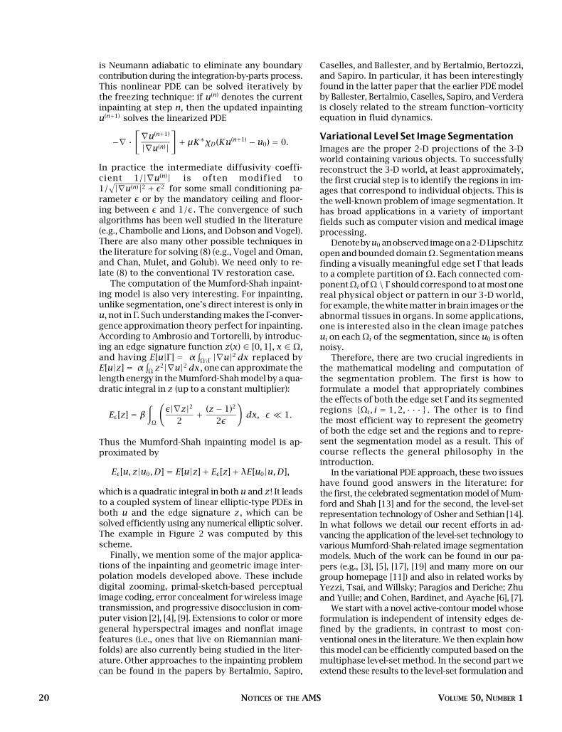
In almost all classical active-contour models, the feature-driven energies relyheavily on the gradient feature |∇u0| or onits smoothed version |∇Gσ ∗ u0| , where Gσ denotes a Gaussian kernel with a smallvariance σ. They work well for detectinggradient-defined edges but fail for moregeneral classes of edges such as the bound-ary of a nebula in some astronomical imagesor the top image in Figure 4.

Our new model, active contours withoutedges, first introduced in [5], is independentof the gradient information and therefore canhandle more general types of edges. Themodel is to minimize the energy

E2[c1, c2, Γ |u0] =∫

int(Γ )|u0(x)− c1|2 dx

+∫

ext(Γ )|u0(x)− c2|2 dx+ ν|Γ |,(9)

where ν denotes a given positive weight, the c’s areunknown constants, int(Γ ) and ext(Γ ) denote the interior and exterior of Γ, and |Γ | is its length. Thesubscript 2 in E2 indicates that it deals with two-phase images, i.e., ones whose “objects” can becompletely indexed by the interior and exterior of Γ.

In the level-set formulation of Osher andSethian [14], Γ is embedded as the zero-level setφ = 0 of a Lipschitz continuous functionφ : Ω → R. Consequently, φ > 0 and φ < 0 de-fine the interior Ω+ and exterior Ω− of the curve.(The level-set approach is computationally superiorto other curve representations, because it lets onedirectly work on a fixed rectangular grid and it allows automatic topological changes such as merg-ing and breaking.) Denote by H the 1-dimensionalHeaviside function: H(z) = 1 if z ≥ 0 and 0 if z < 0.Then the energy in our model becomes

E2[c1, c2,φ|u0] =∫Ω|u0(x)− c1|2H(φ)dx

+∫Ω|u0(x)−c2|2(1−H(φ))dx+ν

∫Ω|∇H(φ)|dx.

Minimizing E2[c1, c2,φ|u0] with respect to c1 , c2 ,and φ leads to the Euler-Lagrange equation:

∂φ∂t

= δ(φ)[νdiv

( ∇φ|∇φ|

)

− |u0 − c1|2 + |u0 − c2|2],

c1(t) =∫Ω u0(x)H(φ(x))dx∫

ΩH(φ(x))dx,

c2(t) =∫Ω u0(x)(1−H(φ(x)))dx∫

Ω(1−H(φ(x)))dx,

with a suitable initial guess φ(0, x) = φ0(x). In nu-merical implementations the Heaviside functionH(z) is often regularized by some Hε(z) in C1(R)that converges as ε → 0 to H(z) in some suitablesense. As a result, the Dirac function δ(z) in the last

Figure 4. Top: Detection of a simulated minefield by our new active-contour model. Bottom: Segmentation of an MRI brain image. Noticethat the interior boundaries are automatically detected.

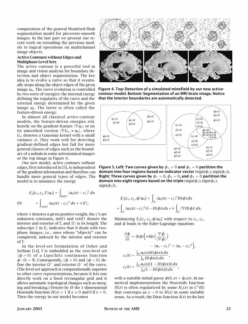
Figure 5. Left: Two curves given by φ1 = 0 and φ2 = 0 partition thedomain into four regions based on indicator vector (sign(φ1),sign(φ2)).Right: Three curves given by φ1 = 0, φ2 = 0, and φ3 = 0 partition thedomain into eight regions based on the triple (sign(φ1),sign(φ2),sign(φ3)).

22 NOTICES OF THE AMS VOLUME 50, NUMBER 1

equation is regularized to δε(z) = H′ε(z). We have

discovered in [5] that a carefully designed approx-imation scheme can even allow interior contours toemerge, a challenging task for most conventionalalgorithms. Also notice that the length term in theenergy has led to the mean-curvature motion.

The model performs as an active contour in theclass of piecewise-constant images taking only twovalues; it looks for a two-phase segmentation of agiven image. The internal energy is defined by thelength, while the external energy is independent ofthe gradient |∇u0|. Defining the segmented imageby u(x) = c1H(φ(x))+ c2(1−H(φ(x))) , we realizethat the energy model is exactly the Mumford-Shahsegmentation model [13] restricted to the class ofpiecewise-constant images. However, our modelwas initially developed from the active-contourpoint of view.

Two typical numerical outputs of the model aredisplayed in Figure 4. The top row shows that ourmodel can segment and detect objects withoutclear gradient edges. The bottom one shows thatit can also capture complicated boundaries andinterior contours.

For more complicated situations where multipleobjects occlude each other and multiphase edgessuch as T-junctions emerge, the above two-phase

active-contour model is insufficient, and we needto introduce multiple level-set functions. Therefore,we have generalized the above framework to multi-phase active contours or, equivalently, the piece-wise-constant Mumford-Shah segmentation withmultiphase regions:

infu,Γ

Ems[u, Γ |u0]

=∑i

∫Ωi|u0 − ci|2 dx+ ν|Γ |.(10)

Here the Ωi’s denote the connected components ofΩ \ Γ , and u = ci on Ωi. Notice that Γ can now be ageneral set of edge curves, including for examplethe T-junction class.

Generally, consider m level-set functionsφi : Ω → R . The union of the zero-level sets of theφi represents the edges in the segmented image.Using these m level-set functions, one can defineup to n = 2m phases, which form a disjoint andcomplete partitioning of Ω. Therefore, each pointx ∈ Ω belongs to one and only one phase. In par-ticular, there is no vacuum or overlap among thephases. This is an important advantage comparedwith the classical multiphase representation, wherea level-set function is associated to each phase andmore level-set functions are needed as a result.Figure 5 shows two typical examples of multiphasepartitioning corresponding to m = 2 and m = 3.

We now illustrate the multiphase level-set ap-proach through the example of n = 4 and m = 2.Let c = (c11, c10, c01, c00) denote a constant vectorand Φ = (φ1,φ2) the two-phase level-set vector.Then we are looking for an ideal image u in the formof

u = c11H(φ1)H(φ2)+ c10H(φ1)(1−H(φ2))

+ c01(1−H(φ1))H(φ2)+ c00(1−H(φ1))(1−H(φ2)).

The Mumford-Shah segmentation energy be-comes

E4[c,Φ|u0] =∫Ω|u0(x)− c11|2H(φ1)H(φ2)dx

+∫Ω|u0(x)− c10|2H(φ1)(1−H(φ2))dx

(11) +∫Ω|u0(x)− c01|2(1−H(φ1))H(φ2)dx

+∫Ω|u0(x)− c00|2(1−H(φ1))(1−H(φ2))dx

+ ν∫Ω|∇H(φ1)|dx+ ν

∫Ω|∇H(φ2)|dx.

Its minimization leads to the Euler-Lagrange equa-tions. First, with Φ fixed, the c minimizer can beexplicitly worked out as before:

Figure 6. The original and segmented images(top row), and the final four segments (the rest).

JANUARY 2003 NOTICES OF THE AMS 23

cij (t) = average of u0 on

(2i − 1)φ1 > 0, (2j − 1)φ2 > 0,i, j = 0,1.

In turn, this new c information leads to the Euler-Lagrange equations for Φ:

∂φ1

∂t= δ(φ1)

[νdiv

( ∇φ1

|∇φ1|)

−((u0 − c11)2 − (u0 − c01)2

)H(φ2)

−((u0 − c10)2 − (u0 − c00)2

)(1−H(φ2))

],

∂φ2

∂t= δ(φ2)

[νdiv

( ∇φ2

|∇φ2|)

−((u0 − c11)2 − (u0 − c01)2

)H(φ1)

−((u0 − c10)2 − (u0 − c00)2

)(1−H(φ1))

].

Notice that the equations are governed both by themean curvatures and by jumps of the data-energyterms across the boundary.

Figure 6 shows an application of the model tothe medical analysis of a brain image. Displayed arethe final segmented image and its associated fourphases. Our model successfully identifies and seg-ments the white and the gray matters.

Recently the above models and algorithms havebeen extended to multichannel, volumetric, andtexture images (e.g., Chan, Sandberg, and Vese [3]).Let us give a little more detail about texture segmentation from our work. Texture images aregeneral images of natural scenes, such as grass-lands, beaches, rocks, mountains, and human bodytissues. They typically carry certain coherent struc-tures in scales, orientations, and local frequencies.To segment texture images using the above mod-els, we first apply Gabor’s filters to extract thesecoherent structures. The filter responses create anew vectorial (or multichannel) feature image in the form of U (x) = (uα(x), uβ(x), · · · , uγ (x)), wherethe Greek letters stand for the filter signatures, andtypically each takes a value of (scale, orientation,local frequency). We then apply the vectorial active-contour-without-edges model to the segmentationof U. Figure 7 shows one typical example.Piecewise-Smooth Mumford-Shah SegmentationThe most general Mumford-Shah piecewise-smoothsegmentation [13] is defined by

(12) infu,Γ

Ems[u, Γ |u0] =∫Ω|u− u0|2 dx

+ µ∫Ω\Γ|∇u|2 dx+ ν|Γ |,

where µ and ν are positive parameters. It allowsthe segmented “objects” to have smoothly varyingintensities instead of being strictly constant. We

now show how to carry out the model based on the

multiphase level-set approach [5]. As before, we

start with the two-phase situation where a single

level-set function φ is sufficient, followed by the

more general multiphase case.

In the two-phase situation, the ideal image u is

segmented to u± by the level-set function φ:

u(x) = u+(x)H(φ(x))+ u−(x)(1−H(φ(x))).

We assume that both u+ and u− are C1 functions

up to the boundary φ = 0. Substituting this ex-

pression into (12), we obtain

E[u+, u−,φ|u0] =∫Ω|u+ − u0|2H(φ)dx

+∫Ω|u−u0|2(1−H(φ))dx

+ µ∫Ω|∇u+|2H(φ)dx

(13)

+ µ∫Ω|∇u−|2(1−H(φ))dx+ ν

∫Ω|∇H(φ)|.

First, with φ fixed, the variation on

E[u+, u−,φ|u0] leads to the two Euler-Lagrange

equations for u± separately:

(14)u± − u0 = µu± on ±φ > 0,

∂u±

∂n= 0 on φ = 0.

(Here ± takes either of the values + and − , but uni-

formly across the formula.) They act as denoising

operators on the homogeneous regions only. No-

tice that no smoothing is done across the bound-

ary φ = 0, which is very important in image

analysis.

Next, keeping the functions u+ and u− fixed and

minimizing E[u+, u−,φ|u0] with respect to φ, we

obtain the motion of the zero-level set:

Figure 7. An example of texture segmentation(at increasing times).

24 NOTICES OF THE AMS VOLUME 50, NUMBER 1

∂φ∂t

= δ(φ)

[ν∇

(∇φ|∇φ|

)− (|u+ − u0|2

+ µ|∇u+|2 − |u−u0|2 − µ|∇u−|2)

],

with some initial guess φ(t = 0, x). The above equa-tion is actually computed at least near a narrowband of the zero-level set. As a result, computa-tionally we have to continuously extend both u+ andu− from their original domains ±φ > 0 to a suit-able neighborhood of the zero-level set φ = 0.Figure 8 displays an application of the model in as-tronomical image analysis. Although the nebulaitself does not seem to be a smooth object, thepiecewise-smooth model can still correctly cap-ture the main features.

As in the previous section, there are cases wherethe boundaries forming a complete partition of theimage cannot be represented by a single level-setfunction. Then one has to turn to the multi-phaseapproach. In our papers, thanks to the planar Four-Color Theorem, we have been able to conclude thattwo level-set functions are sufficient for all multi-phase partition problems.

By the Four-Color Theorem one can color all theregions in a partition using only four colors, so thatany two adjacent regions are color distinguishable.Identifying a phase with one color, we see that twolevel-set functions φ1 and φ2 are sufficient to pro-duce four “colors”: ±φ1 > 0, ±φ2 > 0 . There-fore, they can completely segment a general imagewith a multiphase boundary set Γ given by φ1 = 0or φ2 = 0. As before, we do not have the prob-lems of “overlapping” or “vacuum” as in the worksby Zhao, Chan, Merriman, and Osher. Note that inthis formulation, generally each “color” can stillhave many isolated components. Therefore, thesegmentation is complete only after one applies anextra step of the well-known topological processorfor finding the connected components of an openset.

In this four-phase formulation, the ideal imageu is segmented into four disjoint but completeparts u±±, each defined by one of the four phases:

±φ1 > 0, ±φ2 > 0.Overall, by using the Heaviside function, we obtainthe following synthesis formula:

u =u++H(φ1)H(φ2)+ u+−H(φ1)(1−H(φ2))

+ u−+(1−H(φ1))H(φ2)

+ u−−(1−H(φ1))(1−H(φ2)),

for all x ∈ Ω. We can express the energy functionof u and Φ = (φ1,φ2) in a similar way and derivethe corresponding Euler-Lagrange equations.

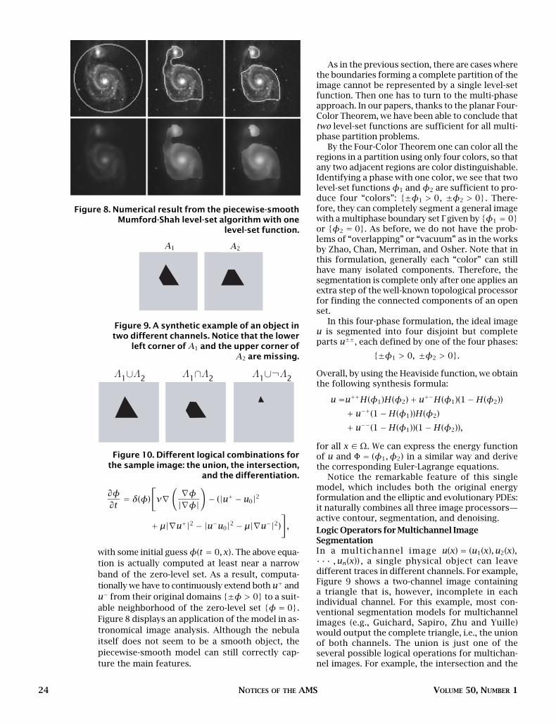
Notice the remarkable feature of this singlemodel, which includes both the original energyformulation and the elliptic and evolutionary PDEs:it naturally combines all three image processors—active contour, segmentation, and denoising.Logic Operators for Multichannel ImageSegmentationIn a multichannel image u(x) = (u1(x), u2(x),· · · , un(x)) , a single physical object can leave different traces in different channels. For example,Figure 9 shows a two-channel image containing a triangle that is, however, incomplete in each individual channel. For this example, most con-ventional segmentation models for multichannelimages (e.g., Guichard, Sapiro, Zhu and Yuille)would output the complete triangle, i.e., the unionof both channels. The union is just one of the several possible logical operations for multichan-nel images. For example, the intersection and the

Figure 8. Numerical result from the piecewise-smoothMumford-Shah level-set algorithm with one

level-set function.

Figure 9. A synthetic example of an object intwo different channels. Notice that the lower

left corner of A1 and the upper corner ofA2 are missing.

A1 A2

Figure 10. Different logical combinations forthe sample image: the union, the intersection,

and the differentiation.

Λ1∪Λ2 Λ1∩Λ2 Λ1∪¬Λ2

A1 A2

JANUARY 2003 NOTICES OF THE AMS 25

differentiation are also very common in applica-tions, as illustrated in Figure 10.

In this section we outline our recent efforts indeveloping logical segmentation schemes for multi-channel images based on the active-contour-without-edges model [16].

First, we define two logical variables to encodethe information inside and outside the contour Γseparately for each channel i:

zini (ui0, x, Γ ) =

1, if x is inside Γ and not onthe object,

0, otherwise;

zouti (ui0, x, Γ ) =

1 if x is outside Γ and onthe object,

0 otherwise.

Such different treatments are motivated by the en-ergy minimization formulation. Intuitively speak-ing, in order for the active contour Γ to evolve andeventually capture the exact boundary of the tar-geted logical object, the energy should be designedso that both partial capture and overcapture leadto high energies (corresponding to zouti = 1 andzini = 1 separately). Imagine that the target objectis tumor tissue: then in terms of decision theory,over and partial captures correspond respectivelyto false alarms and misses. Both are to be penal-ized.

In practice we do not have precise informationof “the object” to be segmented. One possible wayto approximate zini and zouti is based on the inte-rior (Ω+) and exterior (Ω−) averages c±i in channel i:

zini (ui0, x, Γ ) =|ui0(x)− c+i |2

maxy∈Ω+ |ui0(y)− c+i |2,

for x ∈ Ω+, and

zouti (ui0, x, Γ ) =|ui0(x)− c−i |2

maxy∈Ω− |ui0(y)− c−i |2,

for x ∈ Ω−.The desired truth table can then be described

using the zini ’s and zouti ’s. Table 2 shows three ex-amples of logical operations for the two-channelcase. Notice that “true” is represented by 0 insideΓ. The method is designed so as to encourage en-ergy minimization when the contour tries to cap-ture the targeted object inside. Also note that the“zini ” terms and the “zouti ” terms play asymmetricbut complementary roles. For example, the unionA1 ∪A2 corresponds to the union of the “in” termsand the intersection of the “out” terms. Similarly,the intersection A1 ∩A2 corresponds to the inter-section of the “in” terms and the union of the “out”terms.

We then design continuous objective functionsto smoothly interpolate the binary truth table. This

is because in practice, as mentioned above, the z ’sare approximated and take continuous values. Forexample, possible interpolants for the union andintersection are

fA1∪A2 (x) =√zin1 (x)zin2 (x)

+(1−

√(1− zout1 (x))(1− zout2 (x))

),

fA1∩A2 (x) =1−√

(1− zin1 (x))(1− zin2 (x))

+√zout1 (x)zout2 (x).

The square roots are taken to keep the functionsof the same order as the original scalar models. Itis straightforward to extend the two-channel caseto more general n-channel ones.

The energy functional E for the logical objectivefunction f can be expressed by the level set func-tion φ. Generally, as just shown above, the objec-tive function can be separated into two parts,

f = f (zin1 , zout1 , · · · , zinn , zoutn )

= fin(zin1 , · · · , zinn )+ fout (zout1 , · · · , zoutn ).

The energy functional is then defined by

E[φ|c+, c−] = µlength(φ = 0)

+ λ∫Ω

[fin(zin1 , · · · , zinn )H(φ)

+ fout (zout1 , · · · , zoutn )(1−H(φ))]dx.

Here each c± = (c±1 , · · · , c±n ) is in fact a multi-channel vector. The associated Euler-Lagrange equa-tion is similar to the scalar model:

∂φ∂t

= δ(φ)

[µdiv

( ∇φ|∇φ|

)

− λ (fin(zin1 , · · · , zinn )− fout (zout1 , · · · , zoutn ))],

with suitable boundary conditions as before. Eventhough the form often looks complicated for a typ-ical application, its implementation is very similarto that of the scalar model.

Numerical results support our above efforts. Fig-ure 9 shows two different occlusions of a triangle.

Table 2. The truth table for two channels. Notice that inside Γ“true” is represented by 0. It is designed so as to encouragethe contour to enclose the targeted logical object at a lowerenergy cost.

Truth table for the two-channel casezin1 zin2 zout1 zout2 A1 ∪A2 A1 ∩A2 A1 ∩¬A2

x inside Γ(or x ∈ Ω+)

x outside Γ(or x ∈ Ω−)

1 1 0 0 1 1 1

1 0 0 0 0 1 1

0 1 0 0 0 1 0

0 0 0 0 0 0 1

0 0 1 1 1 1 0

0 0 1 0 1 0 1

0 0 0 1 1 0 0

0 0 0 0 0 0 0

26 NOTICES OF THE AMS VOLUME 50, NUMBER 1

We are able to success-fully recover the union,the intersection, and thedifferentiation of the ob-jects in Figure 10 usingour model. In Figure 11we have a two-channelimage of the brain. Inone channel we have a“tumor” with somenoise, while the otherchannel is clear. The im-ages are not registered.We want to findA1 ∩¬A2 so that thetumor can be observed.This happens to be avery complicated exam-ple, as there are a lot offeatures and textures.However, the modelfinds the tumor suc-cessfully.

ConclusionIn this article we have discussed some recent develop-ments in one successful approach to mathematical im-age and vision analysis, the variational PDE method.Besides the inpainting and segmentation problems dis-cussed here, some other problems for which this methodis well suited are adaptive image enhancement and scale-space theory, geometric processing of curves and sur-faces, optical flows of motion pictures, and dynamic ob-ject tracking. Advantages of the method include faithfulmodeling and processing of vision geometry and its re-lated visual optimization, effective simulation of dy-namic visual processes such as selective diffusion andinformation transport, and close interaction with therich literature of numerical analysis and computationalPDEs. This subject shows that mathematics has a key roleto play in addressing real-world problems in scienceand technology. Some challenges for the future are fur-ther theoretical study on the variational and PDE mod-els developed in recent years, more intrinsic integrationwith stochastic modeling and applied harmonic analy-sis such as geometric wavelets, and more systematic in-vestigation on the computation and numerical analysisof geometry-based variational optimizations and PDEs.

AcknowledgmentsJackie Shen thanks his former advisors Gilbert Strang andStan Osher for their constant support and inspiration.

References[1] G. AUBERT and P. KORNPROBST, Mathematical Problems in Image

Processing: Partial Differential Equations and the Calculus

of Variations, Appl. Math. Sci., vol. 147, Springer-Ver-lag, 2001.

[2] T. F. CHAN, S.-H. KANG, and J. SHEN, Euler’s elastica andcurvature based inpaintings, SIAM J. Appl. Math. (2002),in press.

[3] T. F. CHAN, B. SANDBERG, and L. VESE, Active contours with-out edges for vector-valued images, J. Visual Comm.Image Rep. 11 (1999), 130–41.

[4] T. F. CHAN and J. SHEN, Mathematical models for localnontexture inpaintings, SIAM J. Appl. Math. 62 (2001),1019–43.

[5] T. F. CHAN and L. A. VESE, Active contours withoutedges, IEEE Trans. Image Process. 10 (2001), 266–77.

[6] L. COHEN, Avoiding local minima for deformable curvesin image analysis, Proc. 3rd. Internat. Conf. on Curvesand Surfaces (Chamonix-Mont Blanc, 1996), Vol. 1, (A.Le Méhauté, C. Rabut, and L. L. Schumaker, eds.), Van-derbilt Univ. Press, Nashville, TN, 1997, pp. 77–84.

[7] L. COHEN, E. BARDINET, and N. AYACHE, Surface recon-struction using active contour models, Proc. SPIE Conf.on Geometric Methods in Computer Vision, SPIE, Belling-ham, WA, 1993.

[8] M. G. CRANDALL, H. ISHII, and P. L. LIONS, User’s guide toviscosity solutions of second order partial linear dif-ferential equations, Bull. Amer. Math. Soc. (N.S.) 27(1992), 1–67.

[9] S. ESEDOGLU and J. SHEN, Digital inpainting based on theMumford-Shah-Euler image model, European J. Appl.Math. 13 (2002), 353–70.

[10] S. GEMAN and D. GEMAN, Stochastic relaxation, Gibbsdistributions, and the Bayesian restoration of images,IEEE Trans. Pattern Anal. Machine Intell. 6 (1984),721–41.

[11] UCLA Imagers homepage, http://www.math.ucla.edu/~imagers/.

[12] S. MALLAT, A Wavelet Tour of Signal Processing, Aca-demic Press, 1998.

[13] D. MUMFORD and J. SHAH, Optimal approximations bypiecewise smooth functions and associated variationalproblems, Comm. Pure Applied. Math. 42 (1989),577–685.

[14] S. OSHER and J. SETHIAN, Fronts propagating with curvature-dependent speed: Algorithms based onHamilton-Jacobi formulation, J. Comput. Phys. 79(1988), 12–49.

[15] L. RUDIN, S. OSHER, and E. FATEMI, Nonlinear total vari-ation based noise removal algorithms, Physica D 60(1992), 259–68.

[16] B. SANDBERG and T. F. CHAN, Logic operations for active contours on multi-channel images, UCLA Department of Mathematics CAM Report 02-12, 2002.

[17] B. SANDBERG, T. F. CHAN, and L. VESE, A level-set andGabor-based active contour algorithm for segmentingtextured images, UCLA Department of MathematicsCAM report 02-39, 2002.

[18] G. SAPIRO, Geometric Partial Differential Equationsand Image Processing, Cambridge University Press,2001.

[19] L. A. VESE and T. F. CHAN, A multiphase level setframework for image segmentation using the Mumfordand Shah model, UCLA Department of MathematicsCAM Report 01-25, to appear in Internat. J. Comp. Vi-sion (2001).

Figure 11. Region-based logicalmodel on a medical image. In the first

channel, A1, the noisy image has a“brain tumor”, while channel A2 does

not. The goal is to spot the tumorthat is in channel A1 but not in A2, i.e.,

the differentiation A1 ∩¬A2 . In theright-hand column we observe that

the tumor has been successfullycaptured.