DISCRETE AND CONTINUOUS doi:10.3934/dcds.2014.34.477DYNAMICAL SYSTEMSVolume 34, Number 2, February 2014 pp. 477–509

VARIATIONAL DISCRETIZATION

FOR ROTATING STRATIFIED FLUIDS

Mathieu Desbrun

Applied Geometry Lab, Computing + Mathematical Sciences, Caltech

1200 E. California Blvd, Pasadena, CA 91125, USA

Evan S. Gawlik

Computational and Mathematical Engineering, Stanford University450 Serra Mall, Stanford, CA 94305-2004, USA

Francois Gay-Balmaz

CNRS/LMD, Ecole Normale Superieure, Paris, France

24, Rue Lhomond, 75005, Paris, France

Vladimir Zeitlin

LMD, Ecole Normale Superieure, UPMC, Paris, France

24, Rue Lhomond, 75005, Paris, France

(Communicated by Sergei Kuksin)

Abstract. In this paper we develop and test a structure-preserving discretiza-tion scheme for rotating and/or stratified fluid dynamics. The numerical

scheme is based on a finite dimensional approximation of the group of vol-ume preserving diffeomorphisms recently proposed in [25, 9] and is derived

via a discrete version of the Euler-Poincare variational formulation of rotating

stratified fluids. The resulting variational integrator allows for a discrete ver-sion of Kelvin circulation theorem, is applicable to irregular meshes and, being

symplectic, exhibits excellent long term energy behavior. We then report a

series of preliminary tests for rotating stratified flows in configurations thatare symmetric with respect to translation along one of the spatial directions.

In the benchmark processes of hydrostatic and/or geostrophic adjustments,these tests show that the slow and fast component of the flow are correctlyreproduced. The harder test of inertial instability is in full agreement with the

common knowledge of the process of development and saturation of this in-

stability, while preserving energy nearly perfectly and respecting conservationlaws.

1. Introduction. Numerical simulations of rotating stratified flows are of obviousimportance in modeling atmospheric and oceanic dynamics at different spatial andtemporal scales, and are being massively and routinely performed. In spite of con-stant progress in numerical schemes which are successfully used for this purpose,

2010 Mathematics Subject Classification. Primary: 37M15, 37N10; Secondary: 65P10, 37K65.Key words and phrases. Rotating stratified fluids, geometric discretization, Euler-Poincare

formulation, structure-preserving schemes, hydrostatic and geostrophic adjustments.This research was partially supported by a “Projet Incitatif de Recherche” contract from the

Ecole Normale Superieure de Paris, by the Swiss NSF grant 200020-137704, by the U.S. NSF grantCCF-1011944, and by the U.S. Department of Energy grant DE-FG02-97ER25308.

477

478 M. DESBRUN, E. S. GAWLIK, F. GAY-BALMAZ AND V. ZEITLIN

the respect of the intrinsic structure of the equations of fluid motion is rarely dis-cussed or addressed while developing and/or implementing new codes. Yet, in thelimit of infinite Reynolds (or Peclet) number, which is relevant for e.g. large-scaleatmospheric or oceanic flows [26], the equations of motion of the stratified rotatingfluid possess a specific geometric structure [28]—as do the related Euler equations[2, 3]. Physically, this structure manifests itself in specific Lagrangian conserva-tion laws, the most celebrated being the conservation of potential vorticity whichalone allows one to understand many processes taking place in the atmosphere, theocean, or in laboratory experiments (e.g. [16]). We remind the reader that po-tential vorticity, whose Lagrangian conservation follows from Ertel’s theorem, is aquantity constructed by projecting the absolute (i.e. relative plus planetary, whichis due to rotation) vorticity onto the density gradient and dividing the result by thetotal density. Conservation of potential vorticity follows from Kelvin’s circulationtheorem [10]. The existence of a variational (Hamilton’s) principle allows one tointerpret this circulation theorem in terms of the general Noether theorem, link-ing conservation laws to symmetries. Conservation of potential vorticity, thus, isrelated to the symmetry with respect to Lagrangian particle relabeling [28]. Oneshould recall that so-called balanced models in geophysical fluid dynamics, likethe famous quasigeostrophic model [26] (which are extensively used to understandlarge-scale atmospheric and ocean dynamics as well as in climate modeling [23])are an expression of potential vorticity conservation in a certain range of scales.They too possess a (reduced) variational principle [14]. On the other hand, the(non-canonical) Hamiltonian structure of the fluid dynamics equations suggests theuse of so-called symplectic integrators [11] allowing for very accurate long-termconservation of energy.

The question of relevance of the accurate representation of the conservation lawsin a numerical scheme, which should eventually simulate a forced-dissipative realworld, is often debated—but has never been systematically investigated. Somestudies comparing simulation with structure-preserving and standard schemes doshow differences [19], [1]. We believe that capturing conservation laws is in factnumerically crucial, especially in the context of large-scale atmosphere and oceandynamics at extremely high Reynolds numbers, as well as for long-time climaticsimulations.

In this paper, we develop and test a structure-preserving space-time discretiza-tion scheme for rotating and/or stratified fluid dynamics. In order to achieve thisgoal, we use a recently developed structure-preserving discretization for the incom-pressible Euler equations and its extension to incompressible fluids with advectedquantities [25, 9], together with the geometric interpretation of the dynamics ofideal rotating and/or stratified fluids via Euler-Poincare variational principles [13].We will limit ourselves in this paper to models that are symmetric with respect totranslations along one of the spatial directions configurations (so-called 2.5 dimen-sional systems).

The paper is organized as follows. In Section 2, we recall the theory of continuousand discrete Euler-Poincare formulations, the construction of the discrete diffeomor-phism group, and the derivation of the associated structure-preserving discretizationof Euler equations. In Section 3 we derive a structure-preserving discretization fortwo-dimensional non-rotating stratified fluids. We then give a geometric Euler-Poincare formulation of rotating non-stratified (Section 4), and rotating stratified(Section 5) fluids in the 2.5 dimensional situation and use this formulation to derive

VARIATIONAL DISCRETIZATION FOR ROTATING STRATIFIED FLUIDS 479

a structure-preserving discretization. We finally present tests of our new numericalschemes in Section 6.

2. Continuous and discrete Euler-Poincare equations. Our approach is basedon a few essential ingredients. First, we leverage the geometric interpretation (andits underlying variational principle) of the flow of an ideal incompressible fluid as ageodesic on the group of volume-preserving diffeomorphisms of the domain of theflow [2]. This key geometric picture is known to extend to the case where additionalfields are advected by the flow [13], yet interact with it through body forces. Sec-ond, we rely on symplectic integrators [11], obtained via extremization of variationalprinciples [22], to numerically ensure good energy energy behavior as well as exactconservation laws due to Noether’s theorem. Finally, we adopt the construction ofa consistent spatial discretization of the group of volume preserving diffeomorphismrecently proposed in [25], as well as its further developments for incompressiblecontinuum theories [9].

In this section we first recall the formal theory of Euler-Poincare reduction withadvected quantities and the associated circulation theorem, both at the continuousand discrete level. We then review the construction of the discrete volume preservingdiffeomorphism group together with the resulting variational integrator for the Eulerequations of an ideal fluid.

2.1. Euler-Poincare theory with advection. From the work of Arnold (see,e.g., [2]), it is well known that the flow of the Euler equations of an ideal fluidof constant density describes a geodesic on the group of volume preserving diffeo-morphisms of the domain of the fluid, relative to a right invariant L2 Riemannianmetric. More precisely, let us denote by M ⊂ Rn the domain of the fluid (supposedto be compact and with smooth boundary) and denote by Diffvol(M) the group ofall volume preserving diffeomorphisms M . The motion of an incompressible fluid iscompletely characterized by a curve ϕt ∈ Diffvol(M): a particle located at a pointX at time t = 0 travels to x = ϕt(X) at time t. The equations of motion cannaturally be derived from Hamilton’s variational principle

δ

∫ T

0

L(ϕ, ϕ)dt = 0, where L(ϕ, ϕ) =1

2

∫M

|ϕ|2dV.

As this Lagrangian is invariant under particle relabeling, that is, the action ofDiffvol(M) on itself by composition on the right, the variational principle can berewritten in terms of the Eulerian velocity u(x, t) verifying ϕ(X) = u(ϕt(X), t), i.e.u = ϕ ϕ−1. One then obtains the following constrained variational principle

δ

∫ T

0

`(u)dt = 0, where `(u) =1

2

∫M

|u|2dV,

subject to constrained variations δu = v− [v,u], where v is an arbitrary divergencefree vector field and [ , ] is the vector field commutator.

In order to implement the variational integrator based on the discretization ofthe diffeomorphism group, it will be crucial to understand the relation between theLagrangian and the Eulerian variational principle from a more abstract point ofview. This is done by using the theory of Euler-Poincare reduction, see [21], validfor any G-invariant Lagrangian system on a Lie group G. Taking G = Diffvol(M)recovers Arnold’s formulation of ideal fluids, and explains the associated variationalprinciple.

480 M. DESBRUN, E. S. GAWLIK, F. GAY-BALMAZ AND V. ZEITLIN

In the context of geophysical fluid dynamics, there is a new element related to thedensity or (potential) temperature fluctuations interacting with velocity field. Inwhat follows we will use the Boussinesq approximation where these fluctuations areadvected by the flow. Yet, they are coupled to the velocity field through gravity. Theabstract formalism allowing for such a more general situation has been described in[13] and will be of crucial use to derive a variational integrator, as has been done in[9]. The Euler-Poincare theory with advected quantities is briefly reviewed below.

2.1.1. Continuous theory. Let G be a Lie group acting on the right on a vectorspace V . We will denote by

(g, v) ∈ G× V 7→ vg ∈ V and (g, a) ∈ G× V ∗ 7→ ag ∈ V ∗,

the action of G on V and its dual V ∗. The associated infinitesimal actions of theLie algebra g of G are defined by

vξ :=d

dt

∣∣∣∣t=0

v exp(tξ) and aξ :=d

dt

∣∣∣∣t=0

a exp(tξ)

for ξ ∈ g, v ∈ V , a ∈ V ∗, and where exp : g → G denotes the exponential map ofthe Lie group G.

In application to incompressible fluids in a domain M , the group G is the groupDiffvol(M) of all volume preserving diffeomorphisms of M and the space V is suchthat its dual space contains the variables advected by the flow such as buoyancy,entropy, or magnetic field, on which the diffeomorphism group acts by pullback. TheLie algebra g of Diffvol(M) is the space Xdiv(M) of divergence-free vector fields onM , and its dual may be identified with Ω1(M)/dΩ0(M), the space of one-forms onM modulo full differentials.

We now recall from [13] the Euler-Poincare reduction process with advectedquantities. Note that in this paper, we will apply this formalism to fluids bothat the continuous and the discrete level, that is, when the group G is the infinitedimensional group of volume preserving diffeomorphisms or the finite dimensionalgroup of discrete volume preserving diffeomorphisms. It is therefore crucial toformulate this reduction process in the abstract setting, that is, for an arbitraryLie group G. Moreover, this formalism allows us to describe an abstract Kelvincirculation theorem that can be applied both at the continuous and discrete levels.

Theorem 2.1. Assume that the function L : TG × V ∗ → R is right G-invariant,so that upon fixing a0 ∈ V ∗, the Lagrangian La0 : TG → R defined by La0(vg) :=L(vg, a0) is right Ga0-invariant, where Ga0 denotes the isotropy subgroup of a0.Define ` : g× V ∗ → R by

`(vgg−1, a0g

−1) = L(vg, a0).

Given a curve g(t) in G, define ξ(t) := g(t)g(t)−1 ∈ g and a(t) = a0g(t)−1 ∈ V ∗.Then the following are equivalent:

i. With a0 held fixed, Hamilton’s variational principle

δ

∫ T

0

La0(g(t), g(t))dt = 0,

holds, for variations δg(t) of g(t) vanishing at the endpoints.ii. g(t) satisfies the Euler-Lagrange equations for La0 on G.

VARIATIONAL DISCRETIZATION FOR ROTATING STRATIFIED FLUIDS 481

iii. The constrained variational principle

δ

∫ T

0

`(ξ(t), a(t))dt = 0,

holds on g× V ∗, upon using variations of the form

δξ =∂η

∂t− [ξ, η], δa = −aη,

where η(t) ∈ g vanishes at the endpoints.iv. The following Euler-Poincare equations hold on g× V ∗:

∂

∂t

δ`

δξ= − ad∗ξ

δ`

δξ+δ`

δa a, (1)

where : V ∗ × V → g∗ is the bilinear operator defined by

〈v a, ξ〉 = −〈aξ, v〉 , for all v ∈ V , a ∈ V ∗, and ξ ∈ g.

2.1.2. The Kelvin-Noether theorem. The Kelvin-Noether theorem is a version ofNoether’s theorem that holds for solutions of the Euler-Poincare equations. Inparticular, a direct application of this theorem to the Euler equations gives riseto Kelvin’s circulation theorem. We provide here the abstract formulation of theKelvin-Noether theorem, following [13]. Let G be a Lie group which acts from theleft on a manifold C and suppose that K : C ×V ∗ → g∗∗ is an equivariant map, thatis ⟨K(g−1c, ag),Ad∗g µ

⟩= 〈K(c, a), µ〉 , for all g ∈ G, c ∈ C, a ∈ V ∗, and µ ∈ g∗.

Let g(t), ξ(t), a(t) be solutions of the Euler-Poincare equation (1) with an initialadvected parameter a0; further define c(t) := g(t)c0 and

I(t) :=

⟨K(c(t), a(t)),

δ`

δξ(t)

⟩. (2)

Then we have the conservation law

d

dtI(t) =

⟨K(c(t), a(t)),

δ`

δa a(t)

⟩. (3)

In the case of the incompressible Euler equations, the Lie group is G = Diffvol(M)and there is no advected quantity a. The manifold C is the space of loops in thedomain M and the function K : C → Xdiv(M)∗∗ is

〈K(γ), α〉 =

∫γ

α, (4)

where α is a one-form in Ω1(M)/dΩ0(M). So in this case the double dual Xdiv(M)∗∗

is identified with the space of closed loops in M . With these choices (3) recoversthe usual circulation theorem

d

dt

∫γt

u · dx = 0,

where γt is a loop advected by the flow.

482 M. DESBRUN, E. S. GAWLIK, F. GAY-BALMAZ AND V. ZEITLIN

2.1.3. Temporal discretization of Euler-Poincare equations and symplecticity. Wenow describe, following [9], a variational integrator for the Euler-Poincare equations(1). It is adapted from [7] to the case with advected quantities.

Consider a sequence of points g0, g1, ..., gK ∈ G and ξ0, ξ1, ..., ξK−1 ∈ g formingthe discretization of the curves g(t) ∈ G and ξ(t) ∈ g, and fix a time step h. Therelations ξ(t) = g(t)g(t)−1 and a(t) = a0g(t)−1 are discretized as

ξk = τ−1(gk+1g−1k )/h and ak = a0g

−1k ,

where τ : g → G is a local approximant of the exponential map. Such a map τ iscalled a group difference map if it is a local diffeomorphism taking a neighborhoodof 0 ∈ g to a neighborhood of e ∈ G, with τ(0) = e and τ(ξ)−1 = τ(−ξ). Givenξ ∈ g, we denote by dτξ : g→ g the right trivialized tangent map defined as

dτξ(δ) := (Dτ(ξ) · δ) τ(ξ)−1, δ ∈ g.

We use dτ−1ξ : g→ g to refer to the inverse of this map, and(dτ−1ξ

)∗: g∗ → g∗ for

the dual map.The discrete analogue of the action

sa0(g(t)) =

∫ T

0

`(ξ(t), a(t))dt

is given by

sa0d((gk)Kk=0

)=

K−1∑k=0

`(ξk, ak)h,

and the discrete Euler-Poincare equations are obtained by applying the followingdiscrete variational principle

δsa0d((gk)Kk=0

)= 0, (5)

for arbitrary variations δgk of gk such that δg0 = δgK = 0.

Theorem 2.2. Let ` : g → R be a Lagrangian, h a time step and τ : g → G agroup difference map. Then the discrete variational principle (5) yields the updateequations

(dτ−1−hξk

)∗ δ`δξk

=(dτ−1hξk−1

)∗ δ`

δξk−1+ h

δ`

δak ak

ak+1 = akτ(−hξk).

(6)

Being variational, this scheme yields a symplectic integrator, as explained in [22],[9].

2.1.4. Discrete Kelvin-Noether theorem. The discrete analogue of the quantity I(t)defined in (2) is given by

Ik :=

⟨K(ck, ak),

(dτ−1−hξk

)∗ δ`δξk

⟩and the discrete Kelvin-Noether theorem reads as follows:

Theorem 2.3. Suppose that the sequence gk, ξk, ak satisfies the discrete Euler-Poincare equations (6), and define ck := c0g

−1k . Then the quantity Ik satisfies

Ik − Ik−1h

=

⟨K(ck, ak),

δ`

δak ak

⟩.

We refer to [9] for a proof and more explanations.

VARIATIONAL DISCRETIZATION FOR ROTATING STRATIFIED FLUIDS 483

2.2. Discretization of the diffeomorphism group. In order to apply the abovetemporal discretization for numerical simulations of fluid flows, it is necessary tofurther discretize the diffeomorphism group Diffvol(M) by substituting it with afinite dimensional matrix Lie group. This approach, initiated in [25], is recalledhere.

Given a mesh M on the fluid domain M with cells Ci, i = 1, ..., N , define adiagonal N × N matrix Ω consisting of cell volumes: Ωii = Vol(Ci). In [25] it isshown that an appropriate choice of a group to represent discrete volume preservingdiffeomorphisms is the matrix group

D(M) =q ∈ GL(N)+ | q · 1 = 1 and qTΩq = Ω

, (7)

i.e., Ω-orthogonal, signed stochastic matrices. Here 1 denotes the column (1, ..., 1)T

so that the first condition reads∑Nj=1 qij = 1 for all i = 1, ..., N .

We now explain the main idea behind this definition. Consider the linear actionof Diffvol(M) on the space F(M) of functions on M , given by

f ∈ F(M) 7→ f ϕ−1 ∈ F(M), ϕ ∈ Diffvol(M). (8)

The two key properties of this linear map are the following:(1) it preserves the L2 inner product of functions;(2) it preserves the constant functions: C ϕ−1 = C.In the discrete setting, a function is replaced by a vector F ∈ RN , whose value Fion cell Ci is regarded as the cell average of the continuous function. Therefore, thediscrete L2 inner product of two discrete functions is defined by

〈F,G〉0 = FTΩG =

N∑i=1

FiΩiiGi.

The discrete diffeomorphism group (7) is such that its action on discrete functions,i.e. on RN , by matrix multiplication, is an approximation of the linear map (8).It is simple to verify that the conditions q · 1 = 1 and qTΩq = Ω are the discreteanalogues of the conditions (1) and (2) above.

The Lie algebra of D(M), denoted d(M), is the space of Ω-antisymmetric, row-null matrices:

d(M) = A ∈ gl(N) | A · 1 = 0 and ATΩ + ΩA = 0.

The matrices A ∈ d(M) are thus the discrete divergence free vector fields.

Discrete differential forms. As we mentioned above, a discrete function (zero-form) on the mesh is given by a vector F ∈ RN . We will denote by Ω0

d(M) the spaceof discrete functions.

A discrete 1-form on M is an antisymmetric matrix K ∈ so(N). The space ofdiscrete 1-form is denoted by Ω1

d(M). The discrete exterior derivative of a discretefunction F is the discrete 1-form dF given by

(dF )ij := Fi − Fj .

Similarly, discrete 2-forms in Ω2d(M) are given by antisymmetric trilinear forms on

RN . The exterior derivative of a 1-form K ∈ Ω1d(M) is the discrete 2-form

(dK)ijk := Kij +Kjk +Kki.

These definitions, designed to enforce Stokes’ theorem at the discrete level, arecommon to most finite-dimensional notions of exterior calculus (see, e.g., [6, 4, 8]).

484 M. DESBRUN, E. S. GAWLIK, F. GAY-BALMAZ AND V. ZEITLIN

The discrete analogue of the L2 pairing

〈α,X〉 =

∫M

α ·X (9)

between 1-forms α ∈ Ω1(M) and vector fields X ∈ X(M) is given by

〈K,A〉 = Tr(KTΩA), K ∈ Ω1d(M), A ∈ d(M). (10)

Recall that using the L2 pairing (9), the dual space Xdiv(M)∗ can be identified withΩ1(M)/dΩ0(M). Remarkably, this duality holds in the discrete setting, namely,using the discrete L2 pairing (10), we have (see Theorem 2.4 in [9])

d(M)∗ ' Ω1d(M)/dΩ0

d(M).

Adjoint and coadjoint actions, Lie derivatives. Recall that the adjoint andcoadjoint actions of the group Diffvol(M) are given by pushforward and pullbackby the diffeomorphism ϕ:

Adϕ u = ϕ∗u Ad∗ϕ α = ϕ∗α,

where u ∈ Xdiv(M) and α ∈ Ω1(M)/dΩ0(M). The Lie bracket [u,v] on the Liealgebra Xdiv(M) of Diffvol(M) is minus the usual Jacobi-Lie bracket of vector fields

[u,v] = adu v =d

dt

∣∣∣∣t=0

Adϕt v =d

dt

∣∣∣∣t=0

(ϕt)∗v = −£uv,

where £uv is the Lie derivative of v along u.In the discrete setting, that is, for the group D(M), we have the equivalent

formulas

Adq A = qAq−1 Ad∗q K = q−1KΩqΩ−1. (11)

The discrete Lie derivatives of vector fields and 1-forms are thus

£AB = −[A,B] = −(AB −BA) £AK = −[A,KΩ]Ω−1. (12)

Discrete loops. Recall that in the continuous case, the double dual spaceXdiv(M)∗∗ was identified with the closed loops in M via the pairing

〈γ, α〉 =

∮γ

α,

where γ : S1 →M is a closed loop in M and α ∈ Xdiv(M)∗ = Ω1(M)/dΩ0(M). Inthe discrete case, since the space d(M) is finite dimensional, we can simply identifythe double dual d(M) with itself, and consider d(M)∗∗ as the space of discrete loops.This is consistent with Arnold’s treatment of Kelvin circulation theorem, see [5],[25]. The discrete analogue of (4) is thus given by

〈K(Γ),K〉 = 〈Γ,K〉 , Γ ∈ d(M)∗∗, K ∈ Ω1d(M)/dΩ0

d(M). (13)

Nonholonomic constraints. For a smooth curve q(t) ∈ D(M), the matrix A(t) =q(t)q(t)−1 describes the infinitesimal exchanges of fluid particles between any pairsof cells Ci and Cj . For computational efficiency, we further assume that Aij is non-zero only if cells Ci and Cj share a common boundary. This defines a constrainedset S ⊂ d(M),

S = A ∈ d(M) | Aij 6= 0⇒ j ∈ N(i), (14)

where N(i) denotes the set of indices of adjacent cells to cell Ci. Since the Liebracket of A,B ∈ S is not necessarily in S, this constraint is nonholonomic. This

VARIATIONAL DISCRETIZATION FOR ROTATING STRATIFIED FLUIDS 485

constraint will affect the variational principle, since it imposes the use of constrainedvariations. The standard Euler-Poincare variational principle

δ

∫ T

0

`(A)dt = 0, for variations δA = ∂tB + [B,A]

must therefore be replaced by

δ

∫ T

0

`(A)dt = 0, with A ∈ S and (15)

for variations δA = ∂tB + [B,A], B ∈ S.

As shown in [25], the relation between a discrete vector field A ∈ S and thecorresponding continuous vector field u ∈ Xdiv(M) is

Aij ' −1

2Ωii

∫Dij

u · nijdS, (16)

where Dij is the boundary common to cell i and j and nij is the normal vector fieldon Dij pointing from Ci to Cj .

The flat map. A major issue of the discrete approach is to find an approximationof the L2 inner product of divergence free vector fields. In view of the approach weuse, it is more convenient to work on an arbitrary Riemannian manifold M withmetric g. In this setting, the L2 inner product reads∫

M

g(u,v)dx =

∫M

u[ · vdx =⟨u[,v

⟩,

where u[ is the 1-form associated to the vector field u with the Riemannian metricg. Therefore, an approximation of the L2 inner product can be found through theintroduction of a discrete flat operator. If we denote by Mε a mesh with resolutionε, a discrete flat operator is defined as an operator [ : S ⊂ d(M)→ Ω1

d(M) satisfying⟨A[εε , Bε

⟩→ 〈u,v〉⟨

A[εε , [Bε, Cε]⟩→ 〈u, [v,w]〉⟨

A[, B⟩

=⟨B[, A

⟩,

for any Aε, Bε, Cε ∈ S that respectively approximate the continuous vector fieldsu,v,w, where the limit above is taken as ε→ 0.

2.3. Review of the discrete Euler equations. As we already recalled earlier,the Euler equations

∂tu + u · ∇u = −∇p (17)

can be obtained by Euler-Poincare theory (Theorem 2.1) for the group G =Diffvol(M) and for the Lagrangian ` : g = Xdiv(M)→ R given by

`(u) =1

2

∫M

|u|2dx.

In view of the discrete approach used below, it is important to consider the equations(17) as written on a general Riemannian manifold M , with Riemannian metric g.In this case, ∇u is the Levi-Civita covariant derivative of u associated to the metricand ∇p is the gradient of p, taken relative to the Riemannian metric.

486 M. DESBRUN, E. S. GAWLIK, F. GAY-BALMAZ AND V. ZEITLIN

Note that the Euler equations (17) can be equivalently written as

∂tu[ + £uu[ = −dq, (18)

where u[ is the 1-form associated to u using the Riemannian metric on M , £uu[

is the Lie derivative of the one-form u[, and q = p− 12 |u|

2. The equivalence of (17)and (18) follows from the identity

£uu[ = u · ∇u[ +1

2d|u|2.

Spatial discretization. Spatial discretization of the Euler equation is obtainedby considering the discrete Lagrangian ` : d(M)→ R,

`(A) =1

2

⟨A[, A

⟩. (19)

Applying the Euler-Poincare variational principle with nonholonomic constraints(15), we get the equations (

∂tA[ + £AA

[ + dP)ij

= 0 (20)

for all i, j, such that j ∈ N(i). More explicitly, using (12), this reads

∂tA[ij + [A[Ω, A]ij

1

Ωjj= −(Pi − Pj), j ∈ N(i).

Temporal discretization. The discrete Euler-Poincare equations (6) applied tothe discrete diffeomorphism group D(M) and the Lagrangian (19) yields the updateequations ((

dτ−1−hAk

)∗A[k −

(dτ−1hAk−1

)∗A[k−1 + dPk

)ij

= 0, (21)

where τ is a group difference map. A convenient and computationally efficientchoice for τ is the Cayley transform

τ : d(M)→ D(M), τ(A) =

(I − A

2

)−1(I +

A

2

)(22)

and one verifies the formulas(dτ−1A

)∗K =

(I − 1

2£A

)K − 1

4AKΩAΩ−1,

so that (21) reads(A[k −A[k−1

h+

£AkA[k + £Ak−1

A[k−12

+h

4

(Ak−1A

[k−1ΩAk−1Ω−1 −AkA[kΩAkΩ−1

)+ dPk

)ij

= 0.

As explained in [9], cubic terms (matrix products involving three elements of d(M))can be ignored in the above equations, without altering the discrete Kelvin-Noethertheorem that still holds exactly. The discrete equations then reduce to(

A[k −A[k−1h

+£Ak

A[k + £Ak−1A[k−1

2+ dPk

)ij

= 0.

The discrete Kelvin-Noether theorem. We now apply Theorem 2.3 to the caseof the Euler equations. Let C = d(M)∗∗ = d(M) 3 Γ be the space of discrete loopsin M and let D(M) act on C by discrete pullback Γ · q = q−1Γq, see (11). Recall

VARIATIONAL DISCRETIZATION FOR ROTATING STRATIFIED FLUIDS 487

from (13) that the quantity K : C → g∗∗ is given by K(Γ) = Γ. So, the discreteKelvin-Noether Theorem 2.3 says that the quantity

Ik =⟨

Γk,(dτ−1−hAk

)∗A[k

⟩verifies

Ik = Ik−1,

where Γk = Γ0 · q−1k is a discrete loop advected by the discrete fluid flow.

The case of a 2D Cartesian grid. We now compute (20) and (21) for a 2DCartesian grid with uniform spacing ε. Assume that the discrete vector field A ∈ Sapproximates the continuous vector field u = (u, v). If Ci and Cj are horizontallyadjacent cells centered at (a− 1/2, b+ 1/2) and (a+ 1/2, b+ 1/2), then we have

Aij = − 1

2εua,b+1/2

If Ci and Cj are vertically adjacent cells centered at (a + 1/2, b − 1/2) and (a +1/2, b+ 1/2), then we have

Aij = − 1

2εva+1/2,b.

As we have seen, the Lagrangian (19) depends on the choice of an appropriateflat operator. On the 2D Cartesian grid, the operator [ : S → d(M) defined by

A[ij :=

2ε2Aij if j ∈ N(i)

wijε2∑k∈N(i)∩N(j)(Aik +Akj) if j ∈ N(N(i))

(23)

is a discrete flat operator, where wij = 1 if cells Ci and Cj share a single vertex andwij = 2 if cells Ci and Cj belong to the same row or column.

Using (23) and (12), the Lie derivative is, up to an exact discrete differential,(£AA

[)ij

=ε

2

(ωa,bva,b + ωa,b+1va,b+1

)(24)

if Ci and Cj are horizontally adjacent, and(£AA

[)ij

= −ε2

(ωa,bua,b + ωa+1,bua+1,b

)(25)

if Ci and Cj are vertically adjacent. We used the notations

ua,b :=ua,b−1/2 + ua,b+1/2

2, va,b :=

va−1/2,b + va+1/2,b

2

and

ωa,b =ua,b−1/2 + va+1/2,b − ua,b+1/2 − va−1/2,b

ε.

The spatially discretized Euler equations (20) is thus given by∂tu

a,b+1/2 − 12

(ωa,bva,b + ωa,b+1va,b+1

)= − 1

ε

(P a+1/2,b+1/2 − P a−1/2,b+1/2

)∂tv

a+1/2,b + 12

(ωa,bua,b + ωa+1,bua+1,b

)= − 1

ε

(P a+1/2,b+1/2 − P a+1/2,b−1/2)

ua+1,b+1/2 + va+1/2,b+1 − ua,b+1/2 − va+1/2,b = 0.

488 M. DESBRUN, E. S. GAWLIK, F. GAY-BALMAZ AND V. ZEITLIN

The fully discrete (i.e., discrete-space and discrete-time) Euler equations are givenby

ua,b+1/2k −ua,b+1/2

k−1

h − 12

(ωa,b

k va,bk +ωa,b+1

k va,b+1k +ωa,b

k−1va,bk−1+ω

a,b+1k−1 va,b+1

k−1

2

)= − 1

ε

(Pa+1/2,b+1/2k − P a−1/2,b+1/2

k

)va+1/2,bk −va+1/2,b

k−1

h + 12

(ωa,b

k ua,bk +ωa+1,b

k ua+1,bk +ωa,b

k−1ua,bk−1+ω

a+1,bk−1 ua+1,b

k−1

2

)= − 1

ε

(Pa+1/2,b+1/2k − P a+1/2,b−1/2

k

)ua+1,b+1/2k + v

a+1/2,b+1k − ua,b+1/2

k − va+1/2,bk = 0

and correspond to a Crank-Nicholson time update. As explained in [25] this spatialdiscretization of the Euler equations on the regular grid coincides with the Harlow-Welsh scheme [12], albeit with a different time update. Therefore, the variationalscheme can be seen as an extension of this approach to arbitrary grids, offeringthe added bonus of proving a geometric picture. Moreover, this geometric picturehelps extend this scheme to important models of incompressible fluids with advectedquantities, as shown in [25] and as will be done below for stratified rotating fluids,while preserving the attractive properties of the scheme such as its symplecticity, adiscrete Kelvin circulation theorem, and very accurate conservation of energy.

3. 2D stratified flow in the Boussinesq approximation. We now start dis-cussing generalizations of pure Eulerian fluid dynamics by including the effects ofgravity and stratification (variable density). In the presence of gravity, density vari-ations will enter the equation (17) via the buoyancy acceleration. We remind thereader that in the Boussinesq approximation the density variations with respect tosome reference density value (which will be taken to be equal to unity, as in (17))are neglected everywhere except the buoyancy term in the momentum equations.At the same time, mass conservation equations are split into two: the incompress-ibility equation, and the equation of advection of density fluctuations. Below wewill use the full buoyancy variable b = g ρ

ρ0, where ρ0 is background density, g is the

gravitational acceleration, and ρ is density. The equations for incompressible twodimensional Boussinesq flows in the vertical plane thus read

∂tu + u · ∇u + b z = −∇p

∂tb+ u · ∇b = 0, ∇ · u = 0(26)

where u = u(x, z) = (u(x, z), w(x, z)) is the velocity, b = b(x, z) is the buoyancy,p = p(x, z) is the pressure, and z is the vertical unit vector. Note that buoyancyis a Lagrangian invariant. Potential vorticity is identically zero for such system, asvorticity is perpendicular to the (x, z)-plane.

Due to the presence of the buoyancy term in the first equation in (26), a straight-forward linearization around the rest state with constant background stratification(vertical gradient of buoyancy) gives rise to the linear wave solutions—internalgravity waves.

3.1. Geometric formulation. The configuration space for the two dimensionalBoussinesq flow is the group G = Diffvol(M) of volume preserving diffeomorphisms

VARIATIONAL DISCRETIZATION FOR ROTATING STRATIFIED FLUIDS 489

of the vertical domain M under consideration. The buoyancy b is the advectedparameter on which the diffeomorphism group acts on the right by composition:

b · ϕ := b ϕ.The space V ∗ of the general theory (Theorem 2.1) is therefore identified with thespace F(M) of all functions on M , and the infinitesimal action and diamond oper-ation are thus given by

b · u = u · ∇b and v b = b∇v.The fluid Lagrangian ` : g × V ∗ → R is the fluid’s total kinetic energy minus thepotential energy:

`(u, b) =

∫M

(1

2|u|2 − bz

)dx dz.

Using the equalities

δ`

δu= u,

δ`

δb= −z, δ`

δb b = −z b = −b∇z = −b z,

one verifies that the Euler-Poincare equations (1) produce the system (26) (see [13]).Kelvin’s circulation theorem reads

d

dt

∮γt

u · dx = −∮γt

b dz.

It is obtained from the abstract formulation (3) by choosing for C the space of loopsin M and the quantity K : C × V ∗ → g∗∗ given by⟨

K(γ, b),v[⟩

:=

∫γ

v[.

Indeed, one can easily compute that⟨K(γ, b),

δ`

δb b⟩

= −∮γt

b dz.

3.2. Spatial discretization. Consider a mesh M of the fluid domain M . As for theEuler equations, the spatial discretization of the Boussinesq equation is realized byreplacing Diffvol(M) with the finite dimensional groupD(M), and the representationspace F(M) is replaced by the space RN of discrete functions on the mesh M. Adiscrete diffeomorphism is denoted by q ∈ G = D(M) and the discrete buoyancy byB ∈ V ∗ = RN . The duality pairing between V and V ∗ is given by the discrete L2

pairing of functions

〈F,B〉0 = FTΩB =

N∑i=1

FiΩiiBi.

The action by discrete pullback is given by B · q = q−1B, so that the infinitesimalaction of a Lie algebra element A ∈ d(M) and the diamond operation respectivelyread

B ·A = −AB and F B = −(BFT

)a, B, F ∈ RN ,

where (M)a denotes the skew-symmetric part of M . The diamond operation iscomputed as follows:

〈F B,A〉 = −〈B ·A,F 〉0 = 〈AB,F 〉0 = (AB)TΩF = BTATΩF = −FTΩAB

= −Tr(BFTΩA

)= −Tr

((BFT

)aΩA)

= −⟨(BFT

)a, A⟩,

where we used the fact that ΩA for A ∈ d(M) is an antisymmetric matrix.

490 M. DESBRUN, E. S. GAWLIK, F. GAY-BALMAZ AND V. ZEITLIN

The spatially discretized Boussinesq Lagrangian ` : g× V ∗ → R, reads

`(A,B) =1

2

⟨A[, A

⟩− 〈B,Z〉0 , (27)

where the discrete function Z ∈ RN is the discrete analogue of the coordinate z,i.e. Zi is the height of the circumcenter of the cell i. The spatially discretizedEuler-Poincare equations associated to `(A,B) read (

∂tA[ + £AA

[ −(BZT

)a+ dP

)ij

= 0

∂tB −AB = 0,(28)

for all i, j, such that j ∈ N(i).

The case of the Cartesian grid. In this case, we choose Za+1/2,b+1/2 = (b +1/2)ε. If cell i and j are horizontally adjacent we get(

BZT)aij

=1

2

(Ba−1/2,b+1/2Za+1/2,b+1/2 − Za−1/2,b+1/2Ba+1/2,b+1/2

)=ε

2(b+ 1/2)

(Ba−1/2,b+1/2 −Ba+1/2,b+1/2

)=

1

2(ZiBi − ZjBj) =

1

2(Qi −Qj).

If cell i and j are vertically adjacent, we have instead(BZT

)aij

=1

2

(Ba+1/2,b−1/2Za+1/2,b+1/2 − Za+1/2,b−1/2Ba+1/2,b+1/2

)=ε

2

((b+ 1/2)Ba+1/2,b−1/2 − (b− 1/2)Ba+1/2,b+1/2

)=ε

2

((b− 1/2)Ba+1/2,b−1/2 − (b+ 1/2)Ba+1/2,b+1/2

+ Ba+1/2,b−1/2 +Ba+1/2,b+1/2)

=1

2(ZiBi − ZjBj) + εBa+1/2,b =

1

2(Qi −Qj) + εBa+1/2,b,

where we defined the discrete function Qi := ZiBi and we used the notationBa+1/2,b := 1

2

(Ba+1/2,b−1/2 +Ba+1/2,b+1/2

).

Using the relation

Aij = − 1

2εua,b+1/2 resp. Aij = − 1

2εwa+1/2,b

and the formulas (24), resp. (25), we get the spatially discretized Boussinesq equa-tions on a Cartesian grid

∂tua,b+1/2 − 1

2

(ωa,bwa,b + ωa,b+1wa,b+1

)= − 1

ε

(P a+1/2,b+1/2 − P a−1/2,b+1/2

)∂tw

a+1/2,b + 12

(ωa,bua,b + ωa+1,bua+1,b

)+Ba+1/2,b = − 1

ε

(P a+1/2,b+1/2 − P a+1/2,b−1/2)

ua+1,b+1/2 + wa+1/2,b+1 − ua,b+1/2 − wa+1/2,b = 0

∂tBa+1/2,b+1/2 + 1

2ε

(ua+1,b+1/2Ba+3/2,b+1/2 − ua,b+1/2Ba−1/2,b+1/2

+wa+1/2,b+1Ba+1/2,b+3/2 − wa+1/2,bBa+1/2,b−1/2) = 0.(29)

VARIATIONAL DISCRETIZATION FOR ROTATING STRATIFIED FLUIDS 491

3.3. Temporal discretization. The discrete Euler-Poincare equations (6) appliedto the discrete diffeomorphism group D(M) and the Lagrangian (27) yields theupdate equations

((dτ−1−hAk

)∗A[k −

(dτ−1hAk−1

)∗A[k−1 − h

(BkZ

T)a

+ dPk

)ij

= 0

Bk+1 = τ(hAk)Bk

(30)

or, more explicitly,(A[k −A[k−1

h+

£AkA[k + £Ak−1

A[k−12

−(BkZ

T)a

+ dPk

)ij

= 0

Bk+1 = τ(hAk)Bk,

(31)

where cubic terms of elements in d(M) have been ignored as in the Euler equations.On the 2D Cartesian grid, the first equation reads

ua,b+1/2k −ua,b+1/2

k−1

h − 12

(ωa,b

k wa,bk +ωa,b+1

k wa,b+1k +ωa,b

k−1wa,bk−1+ω

a,b+1k−1 wa,b+1

k−1

2

)= − 1

ε

(Pa+1/2,b+1/2k − P a−1/2,b+1/2

k

)w

a+1/2,bk −wa+1/2,b

k−1

h + 12

(ωa,b

k ua,bk +ωa+1,b

k ua+1,bk +ωa,b

k−1ua,bk−1+ω

a+1,bk−1 ua+1,b

k−1

2

)+B

a+1/2,bk = − 1

ε

(Pa+1/2,b+1/2k − P a+1/2,b−1/2

k

).

(32)

Boundary conditions fit naturally into the geometric formulation of the above nu-merical scheme. Tangential boundary conditions are inherent in the nonholonomicconstraints (15), since neighboring cells never share an interface lying on the do-main boundary. In the case of periodic boundary conditions on a Cartesian grid, wemerely identify pairs of cells on opposite boundaries as neighbors in definition (14)of the nonholonomic constraint space S.

These constraints are realized in implementations of (32) on a Cartesian grid ofsize Nx×Nz as follows. For free-slip boundary conditions, the first relation in (32)must hold for 1 ≤ a ≤ Nx − 1, 0 ≤ b ≤ Nz − 1, and the second relation must holdfor 0 ≤ a ≤ Nx − 1, 1 ≤ b ≤ Nz − 1, with the understanding that

u0,b+1/2 = uNx,b+1/2 = ua,−1/2 = ua,Nz+1/2 = 0wa+1/2,0 = wa+1/2,Nz = w−1/2,b = wNx+1/2,b = 0.

For periodic boundary conditions, (32) must hold for 0 ≤ a ≤ Nx − 1, 0 ≤ b ≤Nz − 1, with the understanding that

P−1/2,b+1/2 ≡ PNx−1/2,b+1/2

P a+1/2,−1/2 ≡ P a+1/2,Nz−1/2

B−1/2,b+1/2 ≡ BNx−1/2,b+1/2

Ba+1/2,−1/2 ≡ Ba+1/2,Nz−1/2

uNx,b+1/2 ≡ u0,b+1/2

ua,−1/2 ≡ ua,Nz−1/2

ua,Nz+1/2 ≡ ua,1/2wa+1/2,Nz ≡ wa+1/2,0

w−1/2,b ≡ wNx−1/2,b

wNx+1/2,b ≡ w1/2,b.

492 M. DESBRUN, E. S. GAWLIK, F. GAY-BALMAZ AND V. ZEITLIN

Mixed boundary conditions (e.g., periodic in x and tangential along the upperand lower boundaries) can be handled similarly.Remarks on the implementation. Implementing the temporal update schemeinvolves two stages. First, compute Bk = τ(hAk−1)Bk−1 by solving the linearsystem (

I − hAk−12

)Bk =

(I +

hAk−12

)Bk−1.

Next, compute uk, wk, and Pk by using Newton’s method to solve the system ofnonlinear equations consisting of (32) and the constraint

ua+1,b+1/2k + w

a+1/2,b+1k − ua,b+1/2

k − wa+1/2,bk = 0.

The cost of these two stages is dominated by the second, which amounts to a non-linear solve in approximately 3NxNz unknowns on a grid of size Nx ×Nz. Compu-tational cost of the nonlinear solve is often reduced if the Jacobian is approximatedwith its incomplete LU factorization and held fixed over several Newton iterations(or even over several time steps if the flow is stable).

Discrete circulation theorem. Recall from (13) that the discrete circulation isgiven by the quantity K : C → g∗∗, K(Γ) = Γ. So, the discrete Kelvin-NoetherTheorem 2.3 says that the quantity

Ik =⟨

Γk,(dτ−1−hAk

)∗A[k

⟩verifies

Ik − Ik−1h

=

⟨Γk,

δ`

δBkBk

⟩=⟨

Γk,(BkZ

T)a⟩

,

where Γk = Γ0 · q−1k is a discrete loop advected by the discrete fluid flow.

3.4. Including the second component of velocity. One can include in the2D Boussinesq equations the second component of velocity v in the y-direction asfollows

∂tu + u · ∇u + b z = −∇p

∂tv + u · ∇v = 0

∂tb+ u · ∇b = 0,

(33)

where u = u(x, z) = (u(x, z), w(x, z)) is the velocity in the x and z direction,b = b(x, z) is the buoyancy, and p = p(x, z) is the pressure. Note that we have nowtwo Lagrangian invariants: b and v, and we can construct a new one, the potentialvorticity, as their Jacobian.

These equations are obtained from full 3D Boussinesq equations by supposingthat the flow is symmetric with respect to translations along y; they are thus of-ten referred to as the 2.5D Boussinesq equations. They admit an Euler-Poincaredescription, by taking the same Lagrangian as above

`(u, v, b) =

∫M

(1

2|u|2 − bz

)dxdz

without dependence on v, but using as advected quantities the buoyancy b = b(x, z)and the y-velocity v = v(x, z), on which the diffeomorphism group acts by compo-sition

b 7→ b ϕ v 7→ v ϕ.

VARIATIONAL DISCRETIZATION FOR ROTATING STRATIFIED FLUIDS 493

The spatially discretized equations are thus obtained exactly as above. We letthe discrete diffeomorphism group act on the discrete buoyancy B ∈ RN and thediscrete y-velocity V ∈ RN by discrete pullback, B · q = q−1B and V · q = q−1V ,resulting in the following system of equations

(∂tA

[ + £AA[ −

(BZT

)a+ dP

)ij

= 0

∂tB −AB = 0

∂tV −AV = 0

(34)

for all i, j, such that j ∈ N(i).The temporal discretization is obtained as previously presented: one simply adds

to the system (31) the discrete advection equation

Vk+1 = τ(hAk)Vk.

The Kelvin-Noether theorem, as well as the update equations on the Cartesian grid,are then easily derived.

4. 2.5D rotating Euler equations. We now concentrate on the rotation effects,excluding stratification. We work with 2.5D rotating Euler equations which areobtained from the 3D rotating Euler equations, by supposing that the flow is sym-metric in one spatial direction: ∂y( ) = 0. As the 2.5D Boussinesq equationstreated above, these equations are appropriate as a first approximation while study-ing jets/fronts (non-rotating in the previous case, and non-stratified in the presentcase; we combine both effects in the next Section), which have very different along-front and across-front scales.

The resulting system reads∂tu+ uux + wuz − fv = −px∂tv + uvx + wvz + fu = 0

∂tw + uwx + wwz = −pz,

(35)

with ux + wz = 0 and where u, v, w depend only on (x, z). Here f is the Coriolisparameter, i.e. twice the angular velocity of rotation, which is supposed to bearound the z- axis. In order to derive a variational integrator, we rewrite theseequations in an Euler-Poincare form. This is achieved by using the geostrophicmomentum m := fv + f2x instead of the horizontal velocity v. In terms of m, weget the system

∂tu+ uux + wuz −m = −qx∂tw + uwx + wwz = −qz∂tm+ umx + wmz = 0,

(36)

(see e.g. [24]), where q = p+ 12f

2x2. Note that m is a Lagrangian invariant. The x-derivative of m is also a Lagrangian invariant and represents the potential vorticityfor this translationally symmetric system. The equations are now identical (uponidentifying m with −b) to the Boussinesq equations (26). The internal gravity wavesof the latter become gyroscopic (or inertial) waves in the rotating Euler equations.

494 M. DESBRUN, E. S. GAWLIK, F. GAY-BALMAZ AND V. ZEITLIN

Thus, (36) can be obtained by Euler-Poincare reduction associated to the La-grangian

`(u,m) =

∫ (1

2|u|2 +mx

)dx dz,

where u = (u,w).Kelvin’s circulation theorem,

d

dt

∮γt

u · dx =

∮γt

mdx,

is obtained from the abstract formulation (3) by choosing for C the space of loopsin M and the quantity K : C × V ∗ → g∗∗ given in (4). In terms of the originalvariables, it reads

d

dt

∮γt

u · dx =

∮γt

fv dx.

It is now possible to discretize these equations in the same way as the Boussinesqequations, by using the spatially discretized Lagrangian

`(A,M) =1

2

⟨A[, A

⟩+ 〈M,X〉0 ,

where now the discrete function X ∈ RN is the discrete analogue of the coordinatex. The spatially discretized Euler-Poincare equations associated to `(A,M) read

(∂tA

[ + £AA[ +

(MXT

)a+ dP

)ij

= 0

∂tM −AM = 0,

(37)

for all i, j, such that j ∈ N(i).On a 2D Cartesian grid, we have Xa+1/2,b+1/2 = (a+ 1/2)ε. Therefore, if cell i

and j are horizontally adjacent, we have(MXT

)aij

=1

2(Qi −Qj) + εMa,b+1/2;

if cell i and j are vertically adjacent, we have instead(MXT

)aij

=1

2(Qi −Qj) ,

where Qi = XiMi. Therefore, Eqs. (37) used on a regular grid read

∂tua,b+1/2 − 1

2

(ωa,bwa,b + ωa,b+1wa,b+1

)−Ma,b+1/2

= − 1ε

(P a+1/2,b+1/2 − P a−1/2,b+1/2

)∂tw

a+1/2,b + 12

(ωa,bua,b + ωa+1,bua+1,b

)= − 1

ε

(P a+1/2,b+1/2 − P a+1/2,b−1/2)

ua+1,b+1/2 + wa+1/2,b+1 − ua,b+1/2 − wa+1/2,b = 0

∂tMa+1/2,b+1/2 + 1

2ε

(ua+1,b+1/2Ma+3/2,b+1/2 − ua,b+1/2Ma−1/2,b+1/2

+wa+1/2,b+1Ma+1/2,b+3/2 − wa+1/2,bMa+1/2,b−1/2) = 0.(38)

The temporal discretization can be carried out as previously for the Boussinesqequations.

To recover the discrete evolution of the original variable v, we use a discreteversion of the geostrophic momentum m = fv + f2x, namely M = fV + f2X, toobtain the evolution of the discrete velocity V from the evolution of M .

VARIATIONAL DISCRETIZATION FOR ROTATING STRATIFIED FLUIDS 495

5. 2.5D rotating Boussinesq equations. We now combine the effects of strati-fication and rotation. Again, we apply the Boussinesq approximation and assume aconfiguration rotating with the angular velocity f/2 around the z- axis and invariantwith respect to translations in y- direction. We thus get:

∂tu+ uux + wuz − fv = −px∂tv + uvx + wvz + fu = 0

∂tw + uwx + wwz + b = −pz∂tb+ ubx + wbz = 0,

(39)

with ux + wz = 0.The same change of variable as before, m = fv + f2x, yields the equations

∂tu+ uux + wuz −m = −qx∂tw + uwx + wwz + b = −qz∂tm+ umx + wmz = 0

∂tb+ ubx + wbz = 0

(40)

with ux + wz = 0 and where the modified pressure is q = p + 12f

2x2. Note thatthere are two Lagrangian invariants b and m. The third one, potential vorticity,can be constructed as the Jacobian of these two. Again, straightforward lineariza-tion reveals the presence of linear wave solutions, which are internal inertia-gravitywaves.

The equations (40) can be obtained as Euler-Poincare equations for the La-grangian

`(u,m, b) =

∫ (1

2|u|2 +mx− bz

)dx dz,

where u = (u,w). In this case, there are two advected quantities, m and b on whichthe group Diffvol(M) of volume preserving diffeomorphisms acts by composition onthe right:

m · ϕ = m ϕ, b · ϕ = b ϕ.Kelvin’s circulation theorem reads

d

dt

∮γt

u · dx =

∮γt

mdx−∮γt

b dz.

Being in an Euler-Poincare form, the system (40) can be spatially discretizedusing the Lagrangian

`(A,M,B) =1

2

⟨A[, A

⟩+ 〈M,X〉0 − 〈B,Z〉0 ,

where the discrete functionsX and Z have the same meaning as above. The spatiallydiscretized Euler-Poincare equations associated to `(A,M,B) read

(∂tA

[ + £AA[ −

(BZT

)a+(MXT

)a+ dP

)ij

= 0

∂tM −AM = 0

∂tB −AB = 0

(41)

for all i, j, such that j ∈ N(i).

496 M. DESBRUN, E. S. GAWLIK, F. GAY-BALMAZ AND V. ZEITLIN

On a 2D Cartesian grid, we get

∂tua,b+1/2 − 1

2

(ωa,bwa,b + ωa,b+1wa,b+1

)−Ma,b+1/2

= − 1ε

(P a+1/2,b+1/2 − P a−1/2,b+1/2

)∂tw

a+1/2,b + 12

(ωa,bua,b + ωa+1,bua+1,b

)+Ba+1/2,b

= − 1ε

(P a+1/2,b+1/2 − P a+1/2,b−1/2)

ua+1,b+1/2 + wa+1/2,b+1 − ua,b+1/2 − wa+1/2,b = 0

∂tMa+1/2,b+1/2 + 1

2ε

(ua+1,b+1/2Ma+3/2,b+1/2 − ua,b+1/2Ma−1/2,b+1/2

+wa+1/2,b+1Ma+1/2,b+3/2 − wa+1/2,bMa+1/2,b−1/2) = 0

∂tBa+1/2,b+1/2 + 1

2ε

(ua+1,b+1/2Ba+3/2,b+1/2 − ua,b+1/2Ba−1/2,b+1/2

+wa+1/2,b+1Ba+1/2,b+3/2 − wa+1/2,bBa+1/2,b−1/2) = 0,

(42)

where

Ma,b+1/2 =Ma−1/2,b+1/2 +Ma+1/2,b+1/2

2,

Ba+1/2,b =Ba+1/2,b−1/2 +Ba+1/2,b+1/2

2.

The discrete Kelvin’s (circulation) Theorem 2.3 implies that the quantity

Ik =⟨

Γk,(dτ−1−hAk

)∗A[k

⟩verifies

Ik − Ik−1h

=

⟨Γk,

δ`

δBkBk +

δ`

δMkMk

⟩=⟨

Γk,(BkZ

T)a − (MkX

T)a⟩

,

where Γk = Γ0 · q−1k is a discrete loop advected by the discrete fluid flow.

6. Numerical tests. We now report a series of preliminary tests of the proposednumerical scheme for the three considered configurations, namely for 2D Boussinesqequations and 2.5D rotating Euler equations (to test separately and respectivelyhow the scheme treats stratification and rotation) and finally for 2.5D rotatingBoussinesq equations (where both effects are combined). It is important to bearin mind that in all three cases the system supports internal waves. These aregravity waves in pure stratified case, inertial (or gyroscopic) waves in pure rotatingcase, and inertia-gravity waves in the mixed case. Waves are fast motions, andit is important that the numerical scheme resolves them well. At the same timethe potential-vorticity bearing motions are slow, and the separation of slow andfast motions at small Rossby numbers is one of the paradigms of geophysical fluiddynamics, e.g. [29].

6.1. Hydrostatic adjustment in 2D Boussinesq model. Consider the 2DBoussinesq equations (26) in the vertical plane. If the fluid is in equilibrium, thegravitational term is balanced by the pressure term and we have the hydrostaticbalance:

−b =∂p

∂z.

If the system is out of equilibrium (due, for example, to a localized heating), ittends to a balanced state via the process of hydrostatic adjustment [17] by emittinginternal gravity waves.

VARIATIONAL DISCRETIZATION FOR ROTATING STRATIFIED FLUIDS 497

We test our numerical scheme with the hydrostatic adjustment process. Considerthe hydrostatic equilibrium u(x, z) = w(x, z) = 0 and b(x, z) = −N2z, where N isthe Brunt-Vaisala frequency. The pressure is thus given by p(x, z) = 1

2gN2z2. We

now consider a localized perturbation of buoyancy. More precisely, for the buoyancywe consider the initial value

b0(x, z) = −N2z + b(x, z),

where b(x, z) is a positive function with compact support around a certain point(x0, z0) (localized perturbation). It is known that the frequency of the emittedgravity waves verifies the dispersion relation

ω2 − k2xN2

k2= 0, (43)

where k = (kx, kz) ∈ Z2 is the wave vector. An important properties of thisdispersion relation is its anisotropy, and the fact that wave frequencies are boundedfrom above by N .

To test our variational integrator in this situation, we consider the equations(26) in the domain (x, z) ∈ [0, 24] × [0, 1] with free-slip boundary conditions along[0, 24]×0 and [0, 24]×1, periodicity in x, and take N = 1. The Brunt-Vaisalaperiod, i.e. the minimal period of internal gravity waves is 2π under this scaling.For the buoyancy perturbation, we choose the initial condition

b(x, z) =

−z + β exp

(−r20r20−r2

)if r < r0

−z if r > r0(44)

with r0 = 0.2, β = 0.3, r2 = (x−12)2+(z−0.5)2. Our scheme (32) was implementedon a 384 × 16 grid, from t = 0 to t = 100 with the time step ∆t = 0.5. Long-timeenergy conservation is obtained as expected (Fig. 1) due to the symplecticity of ourintegrator.

The graph Fig. 2 displays the Fourier transform of the time series of the buoyancyb(x, z, t) for t ∈ [0, 100] at various locations (x, z) in the domain. The integers ixand iz are the indices of the cell whose center is the point (x, z), in the 384×16 meshof the domain [0, 24]× [0, 1]. For instance, the cell with (ix, iz) = (192, 8) is near thecenter of the grid and its upper right corner has coordinates (x, z) = (12, 0.5). It isclearly seen that the spectra in all locations sharply drop beyond unity, which is thenon-dimensional value of N , in accordance with (43). A well pronounced maximumat unity in the middle of the domain (middle column), where the initial perturbationwas located, is also consistent with (43), as the group velocity of the waves tendsto zero at ω → N and, hence, the corresponding part of initial perturbation cannotbe evacuated.

The snapshots of the evolution of the buoyancy field in the region [11, 13]× [0, 1]which are presented in Fig. 3 confirm the wave emission from the initial perturba-tion. With our boundary conditions, waves are being reflected from the boundaries,but the initial stages clearly show emission from the localized source.

Finally, Fig. 4 shows the buoyancy averaged over 0 < t < 100. The mean state isstably stratified and horizontally uniform as it should. We repeated the simulationwith different domain geometries, all confirming the standard scenario of hydrostaticadjustment.

Geostrophic adjustment in 2.5D rotating Euler equations. As mentionedin Sect. 4, 2.5D rotating Euler equations are equivalent to 2D Boussinesq equations

498 M. DESBRUN, E. S. GAWLIK, F. GAY-BALMAZ AND V. ZEITLIN

0 20 40 60 80 1000.9998

0.9999

1

1.0001

1.0002Energy

Time

Ene

rgy

/ Ini

tial E

nerg

y

Figure 1. Long-time energy evolution for the hydrostatic adjust-ment problem in 2D Boussinesq model.

under appropriate changes of variables, so the above-discussed simulations apply tothe geostrophic adjustment process, i.e. adjustment of velocity and pressure to thegeostrophic balance, given by the relation

fv =∂p

∂x,

by emitting the gyroscopic waves with dispersion relation

ω2 =f2k2z|k|2

.

6.2. Adjustment in the 2.5D rotating Boussinesq equations. Consider nowthe equation (39). Similarly to what we have seen before, an exact solution isprovided by balancing the Coriolis and gravitational terms by the pressure force(the so-called thermal wind relations):

fv =∂p

∂x, fu = 0, b = −∂p

∂z. (45)

Such a situation is realized for example when u = w = 0, v(x, z) = Kx, b(x, z) =−N2z, p = 1

2Kx2 + 1

2N2z2, with K a constant and N the Brunt-Vaisala frequency.

We consider that such equilibrium state is disturbed by a localized perturbation ofthe buoyancy. In this case, the frequency of the emitted wave verifies the dispersionrelation

ω2 =f(K + f)k2z +N2k2x

|k|2. (46)

This frequency is bounded from above and below. In the simplest case of the absenceof background shear, i.e. K = 0, we have f < ω < N (we assume f < N , which isthe case of the ocean and the atmosphere).

VARIATIONAL DISCRETIZATION FOR ROTATING STRATIFIED FLUIDS 499

0 1 20

0.2

0.4

Frequency (rad/sec)

Mag

nitu

de

ix = 160, iz = 12

0 1 20

0.2

0.4

Frequency (rad/sec)

Mag

nitu

de

ix = 160, iz = 8

0 1 20

0.2

0.4

Frequency (rad/sec)

Mag

nitu

de

ix = 160, iz = 4

0 1 20

0.5

1

1.5

Frequency (rad/sec)

Mag

nitu

de

ix = 192, iz = 12

0 1 20

1

2

Frequency (rad/sec)

Mag

nitu

de

ix = 192, iz = 8

0 1 20

0.5

1

Frequency (rad/sec)

Mag

nitu

de

ix = 192, iz = 4

0 1 20

0.2

0.4

Frequency (rad/sec)

Mag

nitu

de

ix = 224, iz = 12

0 1 20

0.2

0.4

Frequency (rad/sec)

Mag

nitu

de

ix = 224, iz = 8

0 1 20

0.2

0.4

Frequency (rad/sec)

Mag

nitu

de

ix = 224, iz = 4

Figure 2. Frequency spectra of buoyancy at different locationsin the flow domain for the hydrostatic adjustment problem in 2DBoussinesq model.

To illustrate the behavior of our integrator in this situation, we consider theequations (39) on the domain (x, z) ∈ [−1, 2] × [−1, 2], with free-slip boundaryconditions and we take K = 0, f = 1, N = 4. For buoyancy, we choose the sameinitial condition as (44), with r0 = 0.2, β = 0.3, r2 = (x − 0.5)2 + (z − 0.5)2. Ourvariational integrator (42) was implemented on a 96× 96 grid from t = 0 to t = 80with the time step ∆t = 0.2.

Of course, the rigid boundaries prevent inertia-gravity waves from escaping fromthe domain, so the adjusted state may be expected only for time-averaged quantities,the time-averaging obviously filtering rapidly oscillating waves.

In the series of snapshots presented in Fig. 5, we display the evolution of thebuoyancy perturbation b+N2z with superimposed velocity field (u,w) in the region[0, 1]× [0, 1].

Emission of inertia-gravity waves from the initial perturbation is clearly seen,displaying a characteristic “St. Andrew’s cross” pattern [18].

The plots of Fig. 6 display the Fourier transform of the time series for the buoy-ancy b(x, z, t) for t ∈ [0, 80] at various locations (x, z) in the domain. The integersix and iz are the indices of the cell with the center at the point (x, z). Theyclearly show that the frequencies lie in the band 1, 4, i.e. between f and N innon-dimensional terms, confirming the inertia-gravity wave nature of the signal.

500 M. DESBRUN, E. S. GAWLIK, F. GAY-BALMAZ AND V. ZEITLIN

x

z

t = 0.0

11.5 12 12.5

0.2

0.4

0.6

0.8

−0.8

−0.6

−0.4

−0.2

x

z

t = 5.0

11.5 12 12.5

0.2

0.4

0.6

0.8

−0.8

−0.6

−0.4

−0.2

x

z

t = 8.0

11.5 12 12.5

0.2

0.4

0.6

0.8

−0.8

−0.6

−0.4

−0.2

Figure 3. Wave emission in the buoyancy field during the hy-drostatic adjustment problem in 2D Boussinesq. The correspond-ing animation may be viewed at http://www.geometry.caltech.edu/Movies/BoussinesqAIMS/boussinesq4.avi

In the sequence of images presented in Fig. 7 the contour plots showing m(x, z)with superimposed velocity field as a function of time demonstrate the conservationof the geostrophic momentum in the scheme.

The graph Fig. 8 illustrates the excellent long term energy behavior, which isdue to the symplecticity of our scheme.

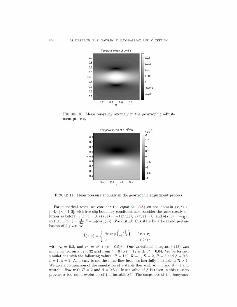
The time averages of the velocity, of the buoyancy anomaly b + N2z (with thebackground stratification removed), and the pressure anomaly p− 1

2N2z (with pres-

sure due to the basic stratification removed), over the interval 0 < t < 80, are pre-sented in Figs. 9, 10, 11. They show very good agreement with the thermal windrelation (45).

VARIATIONAL DISCRETIZATION FOR ROTATING STRATIFIED FLUIDS 501

x

z

Temporal mean of b

11.5 12 12.5

0.2

0.4

0.6

0.8

−0.8

−0.6

−0.4

−0.2

Figure 4. Mean of the buoyancy b during the hydrostatic adjust-ment process 0 < t < 100.

x

z

t = 0.0

0.2 0.4 0.6 0.8

0.1

0.2

0.3

0.4

0.5

0.6

0.7

0.8

0.9

−0.05

0

0.05

0.1

x

z

t = 1.4

0.2 0.4 0.6 0.8

0.1

0.2

0.3

0.4

0.5

0.6

0.7

0.8

0.9

−0.05

0

0.05

0.1

xz

t = 2.8

0.2 0.4 0.6 0.8

0.1

0.2

0.3

0.4

0.5

0.6

0.7

0.8

0.9

−0.05

0

0.05

0.1

Figure 5. Inertia-gravity waves in the buoyancy perturbation dur-ing the geostrophic adjustment in rotating Boussinesq equations.The corresponding animation may be viewed at http://www.

geometry.caltech.edu/Movies/BoussinesqAIMS/both5b+N2z

.avi

The same simulations were carried out with a localized perturbation in v insteadof b, with similar results concerning long term energy behavior and the period ofthe emitted waves was found.

6.3. Inertial instability in 2.5D rotating Boussinesq equations. Having seenthat the numerical scheme reproduces well the basic phenomena in the rotating 2.5D Boussinesq equations we try in this subsection a really hard test of the inertialinstability. The inertial instability is a specific instability of the rotating flows (see,e.g., [15]) appearing in the regions where the product of planetary and potentialvorticities is negative. For positive f (Northern hemisphere) we are using, thismeans that potential vorticity should be negative somewhere in the flow, meaningthat vorticity should be sufficiently negative. Vorticity may be measured by theRossby number of the flow. To make this parameter appear, we rewrite the 2.5Drotating Boussinesq equations (39) in a nondimensional form, that is,

∂tu+R(uux + wuz)− v = −px∂tv +R(uvx + wvz) + u = 0

δ2(∂tw +R(uwx + wwz)) + b = −pz∂tb+R(ubx + wbz) = 0,

(47)

502 M. DESBRUN, E. S. GAWLIK, F. GAY-BALMAZ AND V. ZEITLIN

0 2 4 60

0.1

0.2

Frequency (rad/sec)

Mag

nitu

de

ix = 40, iz = 56

0 2 4 60

0.2

0.4

Frequency (rad/sec)

Mag

nitu

de

ix = 40, iz = 48

0 2 4 60

0.1

0.2

Frequency (rad/sec)

Mag

nitu

de

ix = 40, iz = 40

0 2 4 60

0.5

1

Frequency (rad/sec)

Mag

nitu

de

ix = 48, iz = 56

0 2 4 60

0.5

1

Frequency (rad/sec)

Mag

nitu

de

ix = 48, iz = 48

0 2 4 60

0.5

1

Frequency (rad/sec)

Mag

nitu

de

ix = 48, iz = 40

0 2 4 60

0.2

0.4

Frequency (rad/sec)

Mag

nitu

de

ix = 56, iz = 56

0 2 4 60

0.2

0.4

Frequency (rad/sec)

Mag

nitu

de

ix = 56, iz = 48

0 2 4 60

0.2

0.4

Frequency (rad/sec)

Mag

nitu

de

ix = 56, iz = 40

Figure 6. Frequency spectra of buoyancy during the geostrophicadjustment process at different locations in the domain.

x

z

t = 0.0

0.2 0.4 0.6 0.8

0.1

0.2

0.3

0.4

0.5

0.6

0.7

0.8

0.9

0

0.2

0.4

0.6

0.8

1

x

z

t = 1.4

0.2 0.4 0.6 0.8

0.1

0.2

0.3

0.4

0.5

0.6

0.7

0.8

0.9

0

0.2

0.4

0.6

0.8

1

x

z

t = 2.8

0.2 0.4 0.6 0.8

0.1

0.2

0.3

0.4

0.5

0.6

0.7

0.8

0.9

0

0.2

0.4

0.6

0.8

1

Figure 7. Conservation of the geostrophic momentum during thegeostrophic adjustment in rotating Boussinesq equations. The cor-responding animation may be viewed at http://www.geometry.

caltech.edu/Movies/BoussinesqAIMS/both5m.avi

with ux + wz = 0. Here R = U/fL is the Rossby number, with L the horizontallength scale and U the horizontal velocity scale; δ = H/L is the aspect ratio, withH the vertical length scale; and we choose 1/f as the time scaling. We fix δ = 1.In the present case, the geostrophic momentum is given by m(x, z) = v(x, z) + 1

Rx

VARIATIONAL DISCRETIZATION FOR ROTATING STRATIFIED FLUIDS 503

0 20 40 60 800.9998

0.9999

1

1.0001

1.0002Energy

Time

Ene

rgy

/ Ini

tial E

nerg

y

Figure 8. Energy conservation during the geostrophic adjustmentin rotating Boussinesq equations

x

z

Temporal mean of v

0.2 0.4 0.6 0.8

0.1

0.2

0.3

0.4

0.5

0.6

0.7

0.8

0.9

−0.019

−0.018

−0.017

−0.016

−0.015

−0.014

−0.013

−0.012

Figure 9. Mean v in the geostrophic adjustment process. An ani-mation of the evolution of the velocity v during the geostrophicadjustment process may be viewed at http://www.geometry.

caltech.edu/Movies/BoussinesqAIMS/both5v.avi

and the equations may be rewritten as

∂tu+R(uux + wuz)−m = −qx∂tw +R(uwx + wwz) + b = −qz∂tm+R(umx + wmz) = 0

∂tb+R(ubx + wbz) = 0,

(48)

where q = p+ 12Rx

2.The simplest configuration where inertial instability appears is a barotropic anti-

cyclonic shear with v(x, z) = − tanh(x). It was studied in [27], and we will considerit below.

504 M. DESBRUN, E. S. GAWLIK, F. GAY-BALMAZ AND V. ZEITLIN

x

z

Temporal mean of b+N2z

0.2 0.4 0.6 0.8

0.1

0.2

0.3

0.4

0.5

0.6

0.7

0.8

0.9

−0.01

−0.005

0

0.005

0.01

0.015

0.02

Figure 10. Mean buoyancy anomaly in the geostrophic adjust-ment process.

x

z

Temporal mean of p−N2z2/2

0.2 0.4 0.6 0.8

0.1

0.2

0.3

0.4

0.5

0.6

0.7

0.8

0.9

−2

−1.5

−1

−0.5

0

0.5

1

1.5

2x 10

−3

Figure 11. Mean pressure anomaly in the geostrophic adjustment process.

For numerical tests, we consider the equations (48) on the domain (x, z) ∈[−4, 4]×[−1, 2], with free-slip boundary conditions and consider the same steady so-lution as before: u(x, z) = 0, v(x, z) = − tanh(x), w(x, z) = 0, and b(x, z) = − 1

Rz,

so that p(x, z) = 12Rz

2 − ln(cosh(x)). We disturb this state by a localized pertur-bation of b given by

b(x, z) =

βx exp

(−r20r20−r2

)if r < r0

0 if r > r0,

with r0 = 0.2, and r2 = x2 + (z − 0.5)2. Our variational integrator (42) wasimplemented on a 32× 32 grid from t = 0 to t = 12 with dt = 0.04. We performedsimulations with the following values: R = 1/2, R = 1, R = 2, R = 3 and β = 0.5,β = 1, β = 2. As is easy to see the shear flow becomes inertially unstable at R > 1.We give a comparison of the simulation of a stable flow with R = 1 and β = 1 andunstable flow with R = 2 and β = 0.5 (a lesser value of β is taken in this case toprevent a too rapid evolution of the instability). The snapshots of the buoyancy

VARIATIONAL DISCRETIZATION FOR ROTATING STRATIFIED FLUIDS 505

field b presented in Fig. 12 for the inertially stable configuration clearly illustratehow the perturbation provokes oscillations and emission of inertia-gravity waves,without reorganization of the mean flow.

x

z

t = 0.0

−0.4 −0.2 0 0.2 0.4

0.1

0.2

0.3

0.4

0.5

0.6

0.7

0.8

0.9

−0.9

−0.8

−0.7

−0.6

−0.5

−0.4

−0.3

−0.2

−0.1

x

z

t = 1.0

−0.4 −0.2 0 0.2 0.4

0.1

0.2

0.3

0.4

0.5

0.6

0.7

0.8

0.9

−0.9

−0.8

−0.7

−0.6

−0.5

−0.4

−0.3

−0.2

−0.1

x

z

t = 2.0

−0.4 −0.2 0 0.2 0.4

0.1

0.2

0.3

0.4

0.5

0.6

0.7

0.8

0.9

−0.9

−0.8

−0.7

−0.6

−0.5

−0.4

−0.3

−0.2

−0.1

x

z

t = 3.0

−0.4 −0.2 0 0.2 0.4

0.1

0.2

0.3

0.4

0.5

0.6

0.7

0.8

0.9

−0.9

−0.8

−0.7

−0.6

−0.5

−0.4

−0.3

−0.2

−0.1

x

z

t = 4.0

−0.4 −0.2 0 0.2 0.4

0.1

0.2

0.3

0.4

0.5

0.6

0.7

0.8

0.9

−0.9

−0.8

−0.7

−0.6

−0.5

−0.4

−0.3

−0.2

−0.1

xz

t = 5.0

−0.4 −0.2 0 0.2 0.4

0.1

0.2

0.3

0.4

0.5

0.6

0.7

0.8

0.9

−0.9

−0.8

−0.7

−0.6

−0.5

−0.4

−0.3

−0.2

−0.1

x

z

t = 6.0

−0.4 −0.2 0 0.2 0.4

0.1

0.2

0.3

0.4

0.5

0.6

0.7

0.8

0.9

−0.9

−0.8

−0.7

−0.6

−0.5

−0.4

−0.3

−0.2

−0.1

x

z

t = 7.0

−0.4 −0.2 0 0.2 0.4

0.1

0.2

0.3

0.4

0.5

0.6

0.7

0.8

0.9

−0.9

−0.8

−0.7

−0.6

−0.5

−0.4

−0.3

−0.2

−0.1

x

z

t = 8.0

−0.4 −0.2 0 0.2 0.4

0.1

0.2

0.3

0.4

0.5

0.6

0.7

0.8

0.9

−0.9

−0.8

−0.7

−0.6

−0.5

−0.4

−0.3

−0.2

−0.1

x

z

t = 9.0

−0.4 −0.2 0 0.2 0.4

0.1

0.2

0.3

0.4

0.5

0.6

0.7

0.8

0.9

−0.9

−0.8

−0.7

−0.6

−0.5

−0.4

−0.3

−0.2

−0.1

x

z

t = 10.0

−0.4 −0.2 0 0.2 0.4

0.1

0.2

0.3

0.4

0.5

0.6

0.7

0.8

0.9

−0.9

−0.8

−0.7

−0.6

−0.5

−0.4

−0.3

−0.2

−0.1

x

z

t = 11.0

−0.4 −0.2 0 0.2 0.4

0.1

0.2

0.3

0.4

0.5

0.6

0.7

0.8

0.9

−0.9

−0.8

−0.7

−0.6

−0.5

−0.4

−0.3

−0.2

−0.1

x

z

t = 12.0

−0.4 −0.2 0 0.2 0.4

0.1

0.2

0.3

0.4

0.5

0.6

0.7

0.8

0.9

−0.9

−0.8

−0.7

−0.6

−0.5

−0.4

−0.3

−0.2

−0.1

Figure 12. Evolution of the buoyancy field with superimposedvelocity in the inertially stable case R = 1. Emission of inertia-gravity waves due to initial perturbation is clearly seen. The cor-responding animation may be viewed at http://www.geometry.

caltech.edu/Movies/BoussinesqAIMS/both4_5R1beta1b.avi

506 M. DESBRUN, E. S. GAWLIK, F. GAY-BALMAZ AND V. ZEITLIN

The snapshots of the evolution of the buoyancy field in the simulation of theinertially unstable configuration presented in Fig. 13 clearly show the developmentof the instability, with a formation of “drops” of buoyancy anomalies with associatedvorticity ejected out of the flow in accordance with the convective character of theinertial instability.

x

z

t = 0.0

−0.4 −0.2 0 0.2 0.4

0.1

0.2

0.3

0.4

0.5

0.6

0.7

0.8

0.9

−0.45

−0.4

−0.35

−0.3

−0.25

−0.2

−0.15

−0.1

−0.05

x

z

t = 3.0

−0.4 −0.2 0 0.2 0.4

0.1

0.2

0.3

0.4

0.5

0.6

0.7

0.8

0.9

−0.45

−0.4

−0.35

−0.3

−0.25

−0.2

−0.15

−0.1

−0.05

x

z

t = 5.0

−0.4 −0.2 0 0.2 0.4

0.1

0.2

0.3

0.4

0.5

0.6

0.7

0.8

0.9

−0.45

−0.4

−0.35

−0.3

−0.25

−0.2

−0.15

−0.1

−0.05

x

z

t = 7.0

−0.4 −0.2 0 0.2 0.4

0.1

0.2

0.3

0.4

0.5

0.6

0.7

0.8

0.9

−0.45

−0.4

−0.35

−0.3

−0.25

−0.2

−0.15

−0.1

−0.05

x

z

t = 8.0

−0.4 −0.2 0 0.2 0.4

0.1

0.2

0.3

0.4

0.5

0.6

0.7

0.8

0.9

−0.45

−0.4

−0.35

−0.3

−0.25

−0.2

−0.15

−0.1

−0.05

x

z

t = 11.0

−0.4 −0.2 0 0.2 0.4

0.1

0.2

0.3

0.4

0.5

0.6

0.7

0.8

0.9

−0.45

−0.4

−0.35

−0.3

−0.25

−0.2

−0.15

−0.1

−0.05

Figure 13. Evolution of the buoyancy field (colours) withsuperimposed velocity in the inertially unstable case R =2. Only the part of the calculational domain around ini-tial perturbation is displayed. The corresponding animationmay be viewed at http://www.geometry.caltech.edu/Movies/

BoussinesqAIMS/both4_5R2beta05b.avi

This behavior is consistent with the Lagrangian picture of the inertial instability[15] and with the evolution of the periodic perturbations considered in [27]. Asseen from the evolution of the geostrophic momentum, this evolution leads to aconsiderable reorganization of the mean flow, with eventual homogenization of thegeostrophic momentum at the location of the perturbation. This is fully consis-tent with the general scenario of the evolution of inertial instability [20], yet thedissipationless character of the code allows to capture fine details smeared by thedissipation in the existing simulations of the saturation of the inertial instability.

The energy evolution of the system is presented in Fig. 15. As indicated by thisfigure, the energy is nearly perfectly conserved.

6.4. Conclusions. Our numerical tests showed feasibility of efficient numericalimplementation of the structure-preserving symplectic integrators for Boussinesqequations of rotating stratified fluids. The slow and the fast components of the flowwere correctly reproduced in spite of relatively low resolution; the waves were wellsimulated, their characteristic properties correctly recovered; and the conservationlaws were perfectly verified, with long-term energy conservation. The hard test ofinertial instability showed agreement with common knowledge of the instability. Asfuture work, one may want to leverage upwinding techniques to remove numerical

VARIATIONAL DISCRETIZATION FOR ROTATING STRATIFIED FLUIDS 507

x

z

t = 0.0

−0.4 −0.2 0 0.2 0.4

0.1

0.2

0.3

0.4

0.5

0.6

0.7

0.8

0.9

−0.1

−0.05

0

0.05

0.1

x

z

t = 3.0

−0.4 −0.2 0 0.2 0.4

0.1

0.2

0.3

0.4

0.5

0.6

0.7

0.8

0.9

−0.1

−0.05

0

0.05

0.1

x

z

t = 5.0

−0.4 −0.2 0 0.2 0.4

0.1

0.2

0.3

0.4

0.5

0.6

0.7

0.8

0.9

−0.1

−0.05

0

0.05

0.1

x

z

t = 7.0

−0.4 −0.2 0 0.2 0.4

0.1

0.2

0.3

0.4

0.5

0.6

0.7

0.8

0.9

−0.1

−0.05

0

0.05

0.1

x

z

t = 8.0

−0.4 −0.2 0 0.2 0.4

0.1

0.2

0.3

0.4

0.5

0.6

0.7

0.8

0.9

−0.1

−0.05

0

0.05

0.1

x

z

t = 11.0

−0.4 −0.2 0 0.2 0.4

0.1

0.2

0.3

0.4

0.5

0.6

0.7

0.8

0.9

−0.1

−0.05

0

0.05

0.1

Figure 14. Geostrophic momentum (colours) with superim-posed velocity in the inertially unstable case R = 2.Only the part of the calculational domain around initialperturbation is displayed. The corresponding animationmay be viewed at http://www.geometry.caltech.edu/Movies/

BoussinesqAIMS/both4_5R2beta05M.avi

0 2 4 6 8 10 120.9995

1

1.0005Energy

Time

Energ

y / Initia

l E

nerg

y

Figure 15. Energy behavior in the simulation of the inertiallyunstable case R = 2.

artifacts near sharp gradients of buyoancy without interfering with the structurepreservation of our update equations.

Acknowledgments. The authors thank Jerrold E. Marsden for early inspiration.

508 M. DESBRUN, E. S. GAWLIK, F. GAY-BALMAZ AND V. ZEITLIN

REFERENCES

[1] R. V. Abramov and A. J. Majda, Statistically relevant conserved quantities for truncatedquasigeostrophic flow , Proc. Natl. Acad. Sci. USA., 100 (2003), 3841–3846.

[2] V. I. Arnold, Sur la geometrie differentielle des groupes de Lie de dimenson infinie etses applications a l’hydrodynamique des fluides parfaits, Ann. Inst. Fourier (Grenoble), 16

(1966), 319–361.

[3] V. I. Arnold, “Mathematical Methods in Classical Mechanics,” Springer, New York, 1974.[4] D. N. Arnold, R. S. Falk and R. Winther, Finite element exterior calculus, homological

techniques, and applications, Acta Numerica, 15 (2006), 1–155.

[5] V. I. Arnold and B. A. Khesin, “Topological Methods in Hydrodynamics,” Applied Mathe-matical Sciences, 125, Springer-Verlag, New York, 1998.

[6] A. Bossavit, “Computational Electromagnetism. Variational Formulations, Complementar-

ity, Edge Elements,” Electromagnetism, Academic Press, Inc., San Diego, CA, 1998.[7] N. Bou-Rabee and J. E. Marsden, Hamilton-Pontryagin Integrators on Lie Groups. Part

I: Introduction and Structure-Preserving Properties, Foundations of Computational Math-

ematics, 9 (2009), 197–219.[8] M. Desbrun, E. Kanso and Y. Tong, Discrete differential forms for computational modeling,

in “Discrete Differential Geometry,” Oberwolfach Semin., 38, Birkhauser, Basel, (2008),287–324.

[9] E. S. Gawlik, P. Mullen, D. Pavlov, J. E. Marsden and M. Desbrun, Geometric, variational

discretization of continuum theories, Physica D, 240 (2011), 1724–1760.[10] I. Gjaja and D. D. Holm, Self-consistent Hamiltonian dynamics of wave mean-flow interac-

tion for a rotating stratified incompressible fluid , Physica D, 98 (1996), 343–378.

[11] E. Hairer, C. Lubich and G. Wanner, “Geometric Numerical Integration. Structure-Preserving Algorithms for Ordinary Differential Equations,” Second edition, Springer Series

in Computational Mathematics, 31, Springer-Verlag, Berlin, 2006.

[12] F. H. Harlow and J. E. Welch Numerical calculation of time-dependent viscous incompress-ible flow of fluid with free surface, Physics of Fluids, 8 (1965), 2182–2189.

[13] D. D. Holm, J. E. Marsden and T. S. Ratiu, The Euler-Poincare equations and semidirect

products with applications to continuum theories, Adv. in Math., 137 (1998), 1–81.[14] D. D. Holm and V. Zeitlin, Hamilton’s principle for quasigeostrophic motion, Phys. Fluids,

10 (1998), 800–806.[15] J. R. Holton, “An Introduction to Dynamic Meteorology,” Third edition, Academic Press,

1992.

[16] B. J. Hoskins, M. E. McIntyre and A. W. Robertson, On the use and significance of isentropicpotential vorticity maps, Q. J. R. Met. Soc., 111 (1985), 877–946.

[17] H. Lamb, “Hydrodynamics,” Ch. 309, 310, Dover, 1932.[18] J. Lighthill, “Waves in Fluids,” Ch. 4, Cambridge University Press, Cambridge-New York,

1978.

[19] B. Kadar, I. Szunyogh and Q. J. Devenyi, On the origin of model errors, J. Hung. Meteor.

Soc., 101 (1998), 71–107.[20] R. C. Kloosterziel, P. Orlandi and G. F. Carnevale, Saturation of inertial instability in

rotating planar shear flows, J. Fluid Mech., 583 (2007), 413–422.[21] J. E. Marsden and T. S. Ratiu, “Introduction to Mechanics and Symmetry. A Basic Expo-

sition of Classical Mechanical Systems,” Second edition, Texts in Applied Mathematics, 17,

Springer-Verlag, New York, 1999.

[22] J. E. Marsden and M. West Discrete mechanics and variational integrators, Acta Numer.,10 (2001), 357–514.

[23] J. Marshall and F. Molteni, Toward a dynamical understanding of planetary-scale flowregimes, J. Atmos. Sci., 50 (1993), 1792–1818.

[24] S. Medvedev and V. Zeitlin, Parallels between stratification and rotation in hydrodynamics,

and between both of them and external magnetic field in magnetohydrodynamics, with appli-cations to nonlinear waves, in “IUTAM Symposium on Turbulence in the Atmosphere and

Oceans,” IUTAM Bookseries, 28, Springer, Netherlands, (2010), 27–37.

[25] D. Pavlov, P. Mullen, Y. Tong, E. Kanso, J. E. Marsden and M. Desbrun, Structure-preserving discretization of incompressible fluids, Physica D, 240 (2011), 443–458.

[26] J. Pedlosky, “Geophysical Fluid Dynamics,” Springer, NY, 1979.

VARIATIONAL DISCRETIZATION FOR ROTATING STRATIFIED FLUIDS 509

[27] R. Plougonven and V. Zeiltin, Nonlinear development of inertial instability in a barotropicshear , Physics of Fluids, 21 (2009), 106601.

[28] R. Salmon, “Lectures on Geophysical Fluid Dynamics,” Oxford University Press, New York,

1998.[29] V. Zeitlin, G. M. Reznik and M. Ben Jelloul, Nonlinear theory of geostrophic adjustment.

Part 2. Two-layer and continuously stratified primitive equations, J. Fluid Mech., 491(2003), 207–228.

Received March 2013; revised April 2013.

E-mail address: mathieu@caltech.edu

E-mail address: egawlik@stanford.edu

E-mail address: francois.gay-balmaz@lmd.ens.fr

E-mail address: zeitlin@lmd.ens.fr