Lecture Notes

Valuation

WS 2009Dr. Alex Stomper

Introduction

3

What does this course offer?

Scientific tools and techniques forvaluing financial assets

We focus on• Valuation of publicly traded firms

• Value of equity• Value of total company (debt+equity)

• Valuation of investment projects

Valuation Alex Stomper

4

Relevance of valuation

Valuation and portfolio management• Central role in fundamental analysis• Useful input for technical analysis

Valuation and corporate finance• Corporate objective: value maximization• Capital budgeting• Mergers and aquisitions• Other corporate restructurings

Valuation

5

Valuation and market efficiency(1)

In an „efficient“ market, the market price is thebest estimate of the true value of an asset.

Deviations of market price from true value arerandom.• Weak form: the current price reflects all information in

past prices (i.e., past prices do not help to identifyunder or over value stocks)

• Semi-strong form: the current price reflects all publicinformation

• Strong form: currect price reflects all information,public as well as private.

Valuation

6

Valuation and market efficiency(2)

Strong-form market efficiency is theorecticallyimpossible: Grossman and Stiglitz (1980).

However, the market is usually smarter thanyou think.

Therefore, compare your valuation results withthe market price whenever possible• Do you know something that the market does not

know?• Or do you make a mistake?

Valuation

7

Approaches to valuation

Discounted cashflow valuation, relates thevalue of an asset to the present value ofexpected future cash flows on that asset.

Relative valuation, estimates the value of anasset by looking at the pricing of 'comparable'assets relative to a common variable likeearnings, cash flows, book value or sales.

Real options approach to valuation,quantifies the value of managerial flexibilityusing option pricing models.

Valuation

1. Discount cash flowvaluation

9

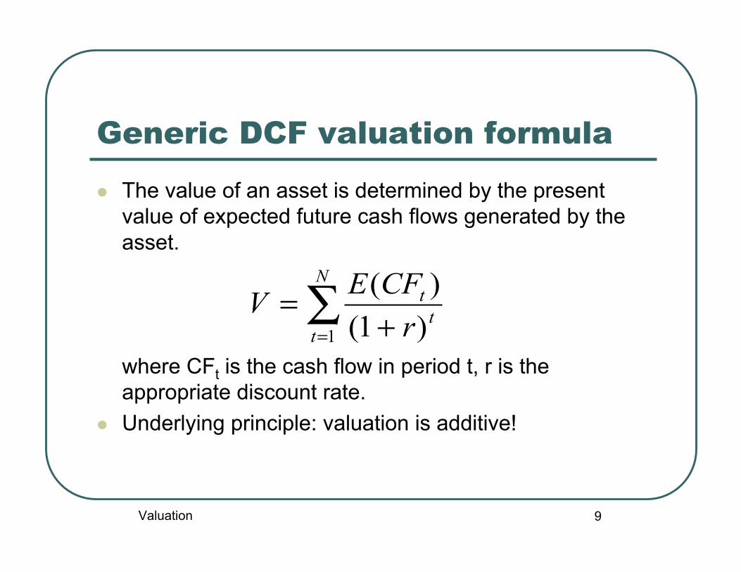
Generic DCF valuation formula

The value of an asset is determined by the presentvalue of expected future cash flows generated by theasset.

where CFt is the cash flow in period t, r is theappropriate discount rate.

Underlying principle: valuation is additive!

∑= +

=N

ttt

rCFEV

1 )1()(

Valuation

10

Key components in DCFvaluation Relevant cash flows

• All cash flows from and to investors (inflows andoutflows)

• Difference between cash flow and profit/loss Appropriate discount rate

• Account for the time value of cash flows (earlier cashflows are more valuable)

• Account for the uncertainty (risk) of cash flows Matching principle: different valuation models

use different combinations of cash flows anddiscount rates.

Valuation

11

DCF valuation models

Free cash flow valuation modelFree cash flow valuation model Capital cash flow valuation model Adjusted present value model Divident discount model Economic-profit-based valuation model

Valuation

12

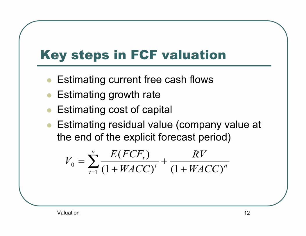
Key steps in FCF valuation

Estimating current free cash flows Estimating growth rate Estimating cost of capital Estimating residual value (company value at

the end of the explicit forecast period)

n

n

tt

t

WACCRV

WACCFCFEV

)1()1()(

10 +

++

=∑=

Valuation

13

I. From earnings to free cashflows EBIT (earnings before interest and taxes)

- Corporate tax rate* EBIT= NOPLAT (net operating profit less adjusted taxes)

+ accounting deductions that did not involve a cash outflow (depreciation,amortization)

- accounting income that did not involve a cash inflow= Gross Cash Flow

- Gross investments (net investment + depreciation)

= Free Cash Flow

- (1-Corporate tax rate)* Interest expense

- Repayment of principal

= Free Cash Flow to Shareholders

Valuation

14

Firm value vs equity value

Value of firm:

Value of equity

∑= +

=N

tt

t

WACCFCFEV

1 )1()(

∑= +

=N

tt

e

t

kFCFEEE

1 )1()(

Valuation

15

Taxes in FCF valuation FCF are calculated as if firms are all-equity

financed Marginal corporate tax rate is applied to EBIT,

without taking into account that interestpayments are tax deductiable

Debt tax shields are recognized through thediscount rate

Alternatively, one can include the debt taxshields in cash flows, then the discount rateshould be the pretax discount rate (Capitalcash flow valuation model, see later).

Valuation

16

Investment expenditures Gross investment

= capital expenditures + change in working capital Working capital = current assets (inventory, cash and

account receivable) - current liabilities (account payable,short-term debt)

Capital expenditures minus depreciation is called netcapital expenditures

Gross investment minus depreciation is called netinvestment

If depreciation is the only noncash expense/income thenFCF = NOPLAT - net investment

Valuation

17

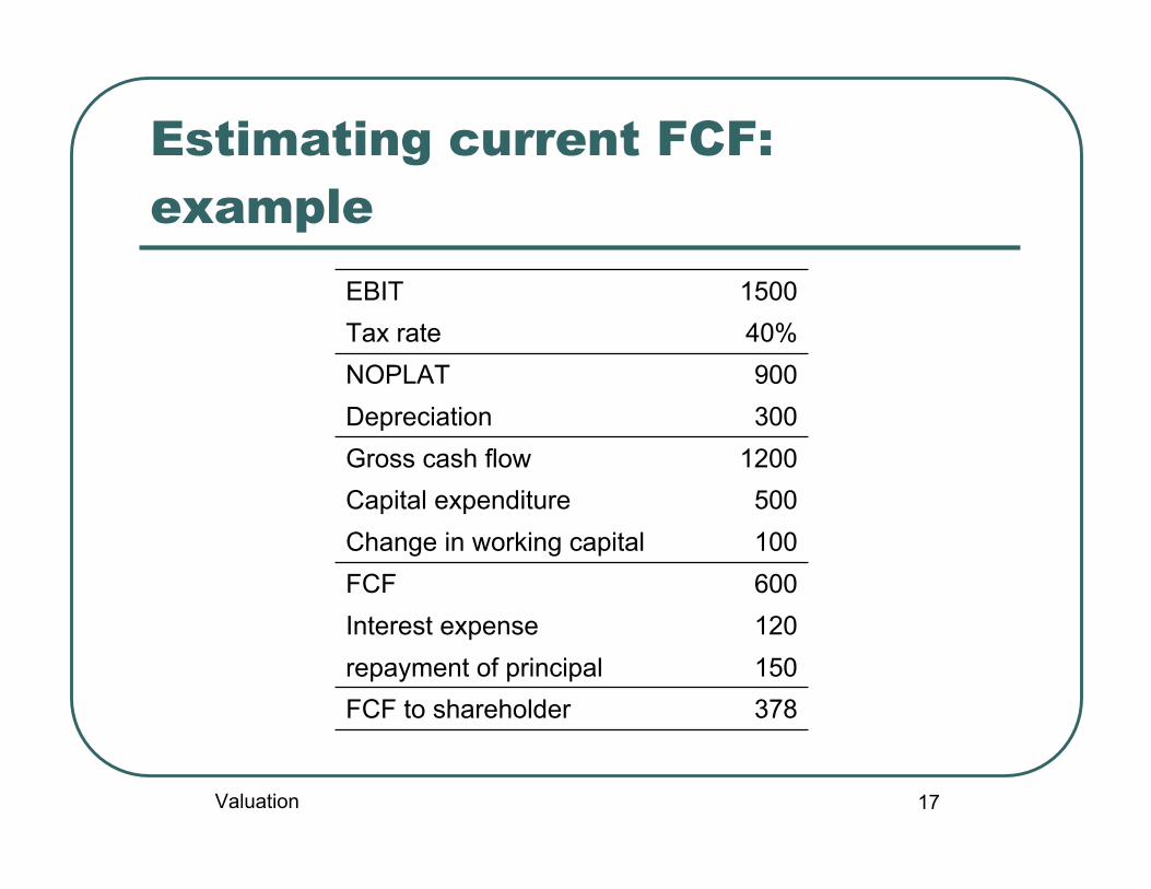
Estimating current FCF:example

EBIT 1500Tax rate 40%NOPLAT 900Depreciation 300Gross cash flow 1200Capital expenditure 500Change in working capital 100FCF 600Interest expense 120repayment of principal 150FCF to shareholder 378

Valuation

18

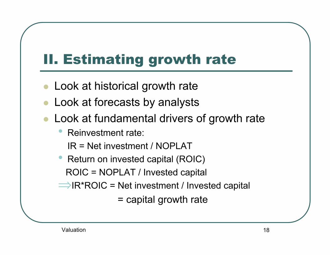
II. Estimating growth rate

Look at historical growth rate Look at forecasts by analysts Look at fundamental drivers of growth rate

• Reinvestment rate:IR = Net investment / NOPLAT

• Return on invested capital (ROIC) ROIC = NOPLAT / Invested capital⇒IR*ROIC = Net investment / Invested capital

= capital growth rate

Valuation

19

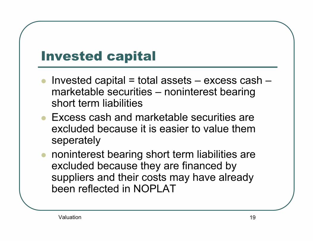
Invested capital

Invested capital = total assets – excess cash –marketable securities – noninterest bearingshort term liabilities

Excess cash and marketable securities areexcluded because it is easier to value themseperately

noninterest bearing short term liabilities areexcluded because they are financed bysuppliers and their costs may have alreadybeen reflected in NOPLAT

Valuation

20

ROIC: example

NOPLAT in year t 900total asset at the end of year t-1 3000excess cash (t-1) 20marketable security (t-1) 100noninterest-bearing liabilities (t-1) 150Invested capital at the end of year

t-1 2730ROIC in year t 0.3

Valuation

21

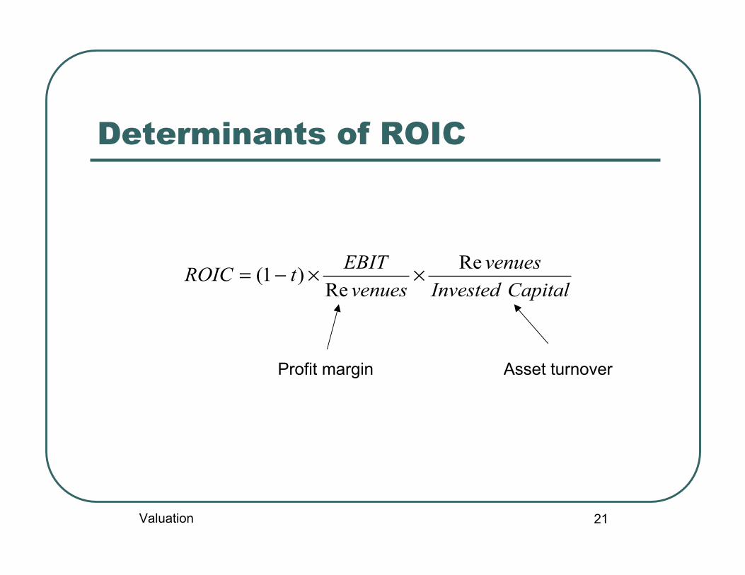
Determinants of ROIC

CapitalInvestedvenues

venuesEBITtROIC Re

Re)1( ××−=

Profit margin Asset turnover

Valuation

22

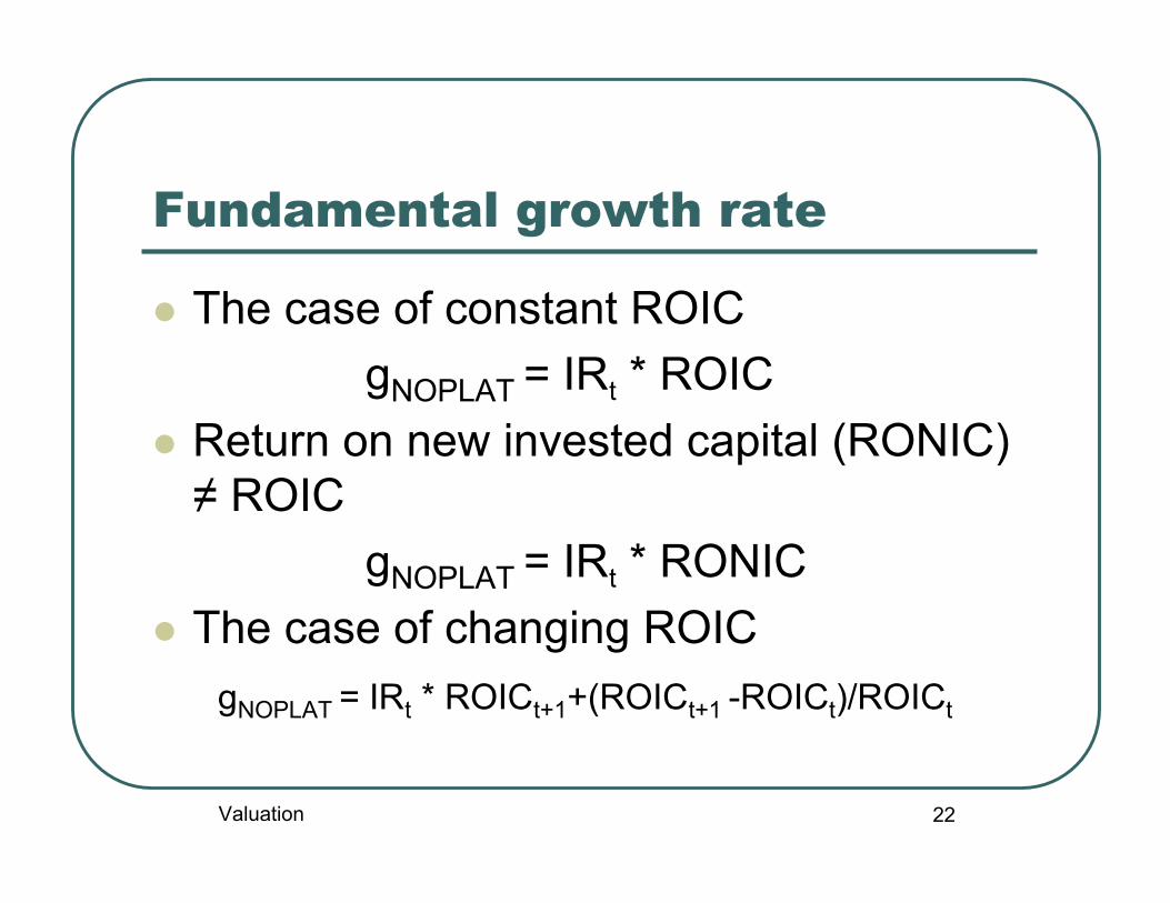
Fundamental growth rate

The case of constant ROIC gNOPLAT = IRt * ROIC

Return on new invested capital (RONIC)≠ ROIC

gNOPLAT = IRt * RONIC The case of changing ROIC

gNOPLAT = IRt * ROICt+1+(ROICt+1 -ROICt)/ROICt

Valuation

23

Forecasting FCFs: example

year 2004 2005 2006 averageinvested capital(beginning) 400.00 450.00 530.00

NOPLAT 150.00 200.00 205.00

ROIC 0.38 0.44 0.39 0.40

Net investment 50.00 80.00 70.00

IR 0.33 0.40 0.34 0.36

FCF 100.00 120.00 135.00

Valuation

24

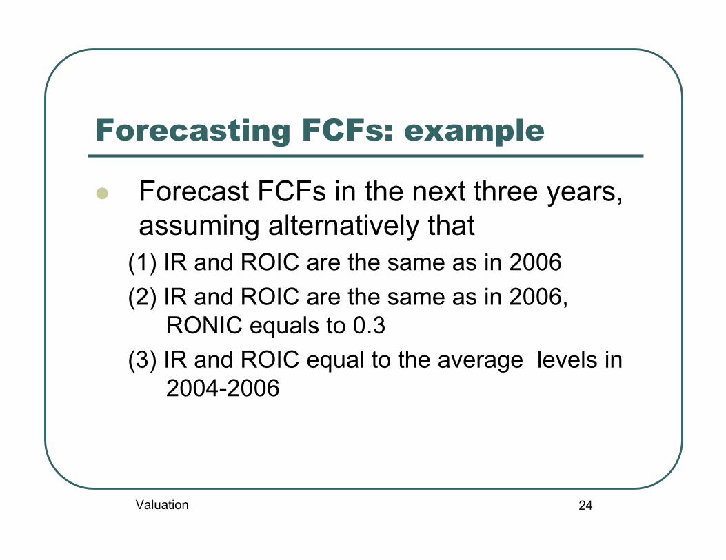
Forecasting FCFs: example

Forecast FCFs in the next three years,assuming alternatively that

(1) IR and ROIC are the same as in 2006(2) IR and ROIC are the same as in 2006,

RONIC equals to 0.3(3) IR and ROIC equal to the average levels in

2004-2006

Valuation

25

Forecasting FCFs: solution

Valuation

26

III. Estimating cost of capital

The expected FCFs to the firm are discounted usingthe weighted average cost of capital (WACC) toget the firm value.

The expected FCFs to equityholders are discountedusing cost of equity to get the equity value.

The weight of each financing form is defined as theratio between the market value of that financing formto the total market value of the firm.

Noninteresting-bearing liabilities are not consideredwhen computing WACC.

The tax advantage of debt financing is reflected inWACC.

Valuation

27

WACC

where kd = pre-tax cost of debt kp = cost of preferred stock ke = cost of equity t = corporate tax rate D/V = target debt ratio using market values P/V = target preferred stock ratio using market values E/V = target equity ratio using market values V = market value of the firm (D+P+S)

VEk

VPk

VDtkWACC epd ++−= )1(

Valuation

28

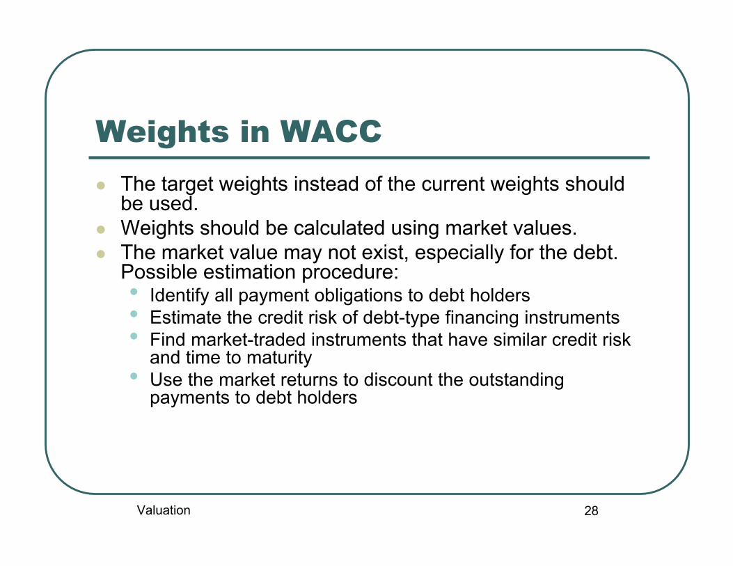
Weights in WACC The target weights instead of the current weights should

be used. Weights should be calculated using market values. The market value may not exist, especially for the debt.

Possible estimation procedure:• Identify all payment obligations to debt holders• Estimate the credit risk of debt-type financing instruments• Find market-traded instruments that have similar credit risk

and time to maturity• Use the market returns to discount the outstanding

payments to debt holders

Valuation

29

Cost of debt/preferred stocks Cost of debt = expected return on debt *(1-t)

• Expected return on debt ≠ coupon rate• Expected return on debt ≠ promised yield

Investment-grade debt (debt rated at BBB or better): useyield to maturity of the company‘s long-term, option-freebonds

If the bond rarely trades, use the average yield to maturityon a portfolio of long term bonds with the same creditrating

Below-investment-grade debt: use CAPM to estimate theexpected return

Adjust for interest tax shields Preferred stocks: preferred dividend devided by the

market price of preferred stocks

Valuation

30

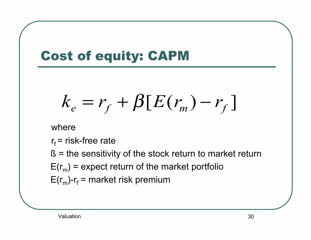
Cost of equity: CAPM

whererf = risk-free rate

ß = the sensitivity of the stock return to market return E(rm) = expect return of the market portfolio E(rm)-rf = market risk premium

])([ fmfe rrErk −+= β

Valuation

31

CAPM: implementation (1)

Risk-free rate: use long-term goverment bond Market risk premium: historical data

• Use the longest period possible: short-term estimatesare very noisy (annual standard deviation of stockreturns 20%).

• Use geometric average instead of arithmetic average• Adjust for survivorship bias.• Nomally used numbers: 4.5-5.5%

Valuation

32

CAPM: implementation (2)

Beta: estimated from the market model

• Normally five-year monthly data are used• Adjustment for low trading frequency (Dimson(1979))

Market portfolio• In theory, all assets must be included• In practice, well-diversified stock indexes are used as a

proxy: S&P 500, MSCI world index, MSCI Europe index,etc

itmtit rr εβα ++=

Valuation

33

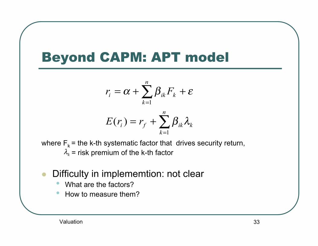
Beyond CAPM: APT model

where Fk = the k-th systematic factor that drives security return, = risk premium of the k-th factor

Difficulty in implememtion: not clear• What are the factors?• How to measure them?

∑

∑

=

=

+=

++=

n

kkikfi

n

kkiki

rrE

Fr

1

1

)( λβ

εβα

kλ

Valuation

34

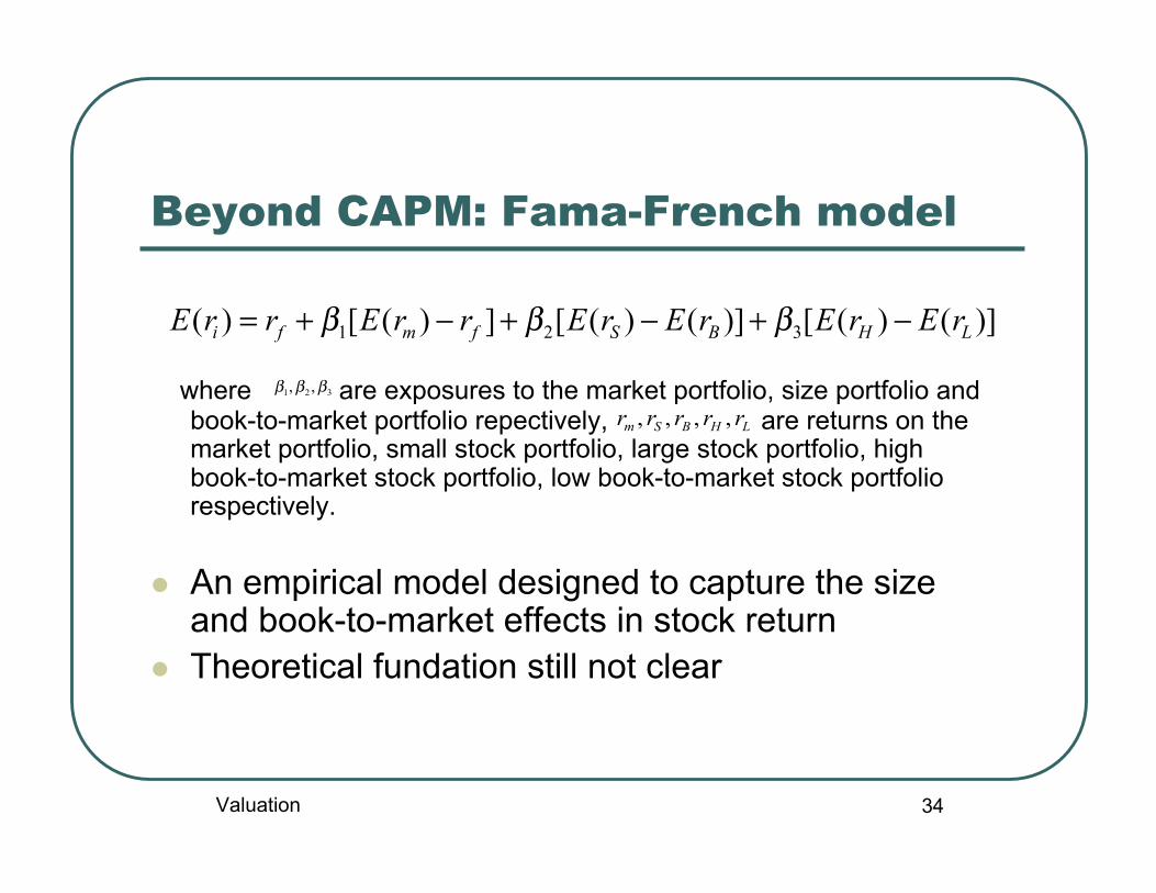
Beyond CAPM: Fama-French model

where are exposures to the market portfolio, size portfolio andbook-to-market portfolio repectively, are returns on themarket portfolio, small stock portfolio, large stock portfolio, highbook-to-market stock portfolio, low book-to-market stock portfoliorespectively.

An empirical model designed to capture the sizeand book-to-market effects in stock return

Theoretical fundation still not clear

321 ,, βββ

)]()([)]()([])([)( 321 LHBSfmfi rErErErErrErrE −+−+−+= βββ

LHBSm rrrrr ,,,,

Valuation

35

Capital structure and cost ofcapital Modigliani and Miller theorem: In a perfect market without tax,

capital structure has no impact on either the firm value or the costof capital.

An easy way to understand this fundamental result in corporatefinance: In a perfect market without tax, capital structure has noimpact on the expected cash flows to the firm.

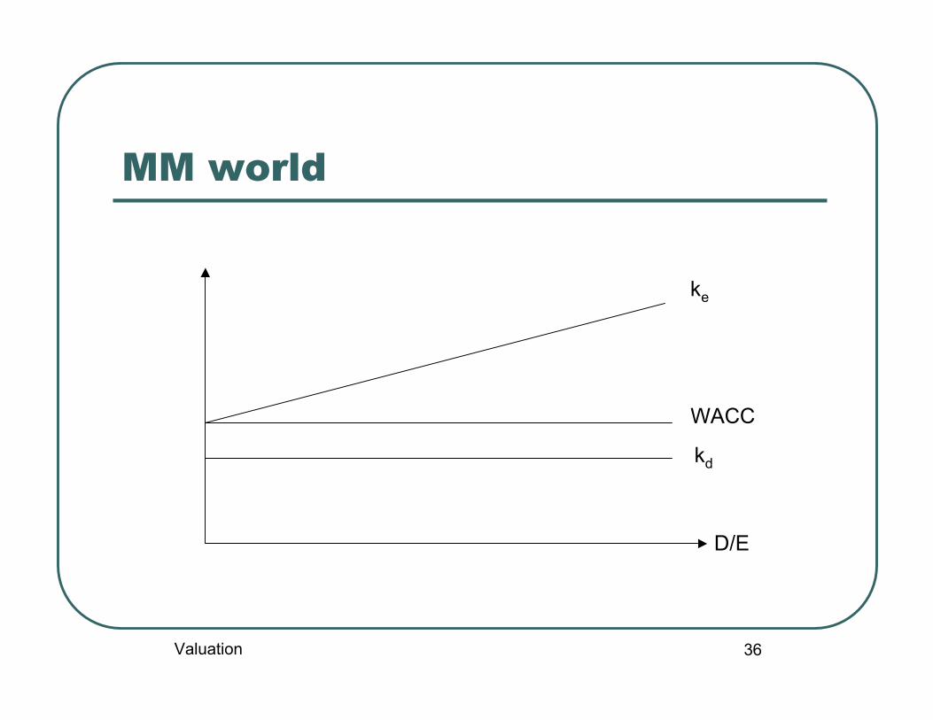
In the MM world, when the more expensive equity is substituted bythe less expensive debt, the cost of equity increases according,leaving the weighted cost of capital unchanged.

In a world with tax, debt increases the cash flows to the firm byreducing taxes. This is not reflected in FCFs, therefore it must bereflect in WACC.

In the real world (with both tax and market imperfections), anoptimal capital structure is determined by the trade-off between thetax advantage of debt and the cost of high leverage.

Valuation

36

MM world

D/E

kd

WACC

ke

Valuation

37

MM world with corporate tax

D/E

kd(1-t)

WACC

ke

Valuation

38

Real world with tax and other frictions

D/E

kd(1-t)

WACC

ke

D/E

kd(1-t)

ke

(D/E)*

Valuation

39

Leverage and equity beta

Industry beta is often used to improve theestimation of company beta.

However, firms in the same industry may havedifferent leverage ratio

Procedure for inferring beta from comparablefirms• Estimate beta for each comparable firm• Back out the unlevered beta• Calculate the relevered beta using the target leverage

ratio

Valuation

Two alternative leverage policies

The relation between levered- and unlevered-betadepends on the assumed leverage policy.

MM assumption(Modigliani and Miller 1963): constantdebt value

ME assumption (Miles-Ezzell 1980): constant debt ratio Note that ME assumption is different from MM

assumption even if expected growth rate is zero. Failing to recognize this difference has led to confusion

even among experts (Fernandez 2004, Cooper andNyborg 2006)

40Valuation

41

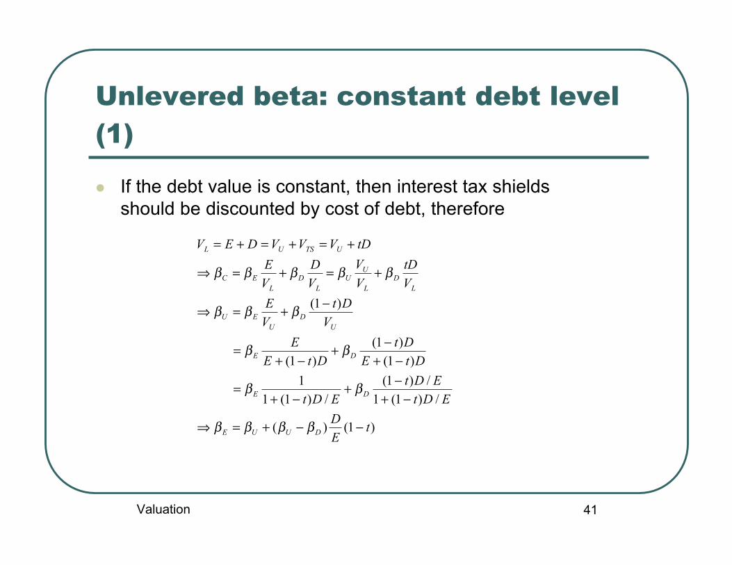
Unlevered beta: constant debt level(1)

If the debt value is constant, then interest tax shieldsshould be discounted by cost of debt, therefore

)1()(

/)1(1/)1(

/)1(11

)1()1(

)1(

)1(

tED

EDtEDt

EDt

DtEDt

DtEE

VDt

VE

VtD

VV

VD

VE

tDVVVDEV

DUUE

DE

DE

UD

UEU

LD

L

UU

LD

LEC

UTSUL

−−+=⇒

−+−+

−+=

−+−+

−+=

−+=⇒

+=+=⇒

+=+=+=

ββββ

ββ

ββ

βββ

βββββ

Valuation

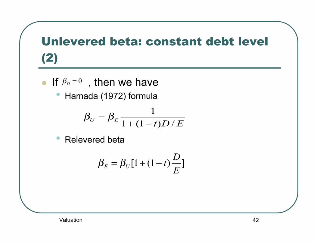
42

Unlevered beta: constant debt level(2)

If , then we have• Hamada (1972) formula

• Relevered beta

0=Dβ

EDtEU /)1(11−+

= ββ

])1(1[EDtUE −+= ββ

Valuation

43

Unlevered (levered) cost ofequity

Unlevered cost of equity can be derivedeither using unlevered beta or directlyfrom the following formula

)1(

)1()(

/)1(1/)1(

/)1(11

DEtDkWACC

tEDkkkk

EDtEDtk

EDtkk

uL

duue

deu

+−==>

−−+=⇒

−+−+

−+=

Valuation

44

Unlevered beta: example

A privately-held company has a leverage ratio(D/E) of 60%.

A comparable publicly-traded company with aleverage ratio of 40% has an equity beta of 1.2.

The comparable firm is assumed to maintainthe current debt level (in value) in the future.

The corporate tax rate is 35%. What is the beta of equity for the private

company?

Valuation

45

Unlevered beta: solution

Valuation

46

Unlevered beta: constant debt ratio(1)

If the debt ratio is constant, then interest taxshields should be discounted usingunlevered cost of equity, therefore

WACCpretaxED

DkED

Ekk

EDD

EDE

VV

VV

VD

VE

VVDEV

DEu

DEU

UL

TSU

L

UU

LD

LEC

TSUL

=+

++

=⇒

++

+=⇒

=+=+=⇒

+=+=

βββ

ββββββ

Valuation

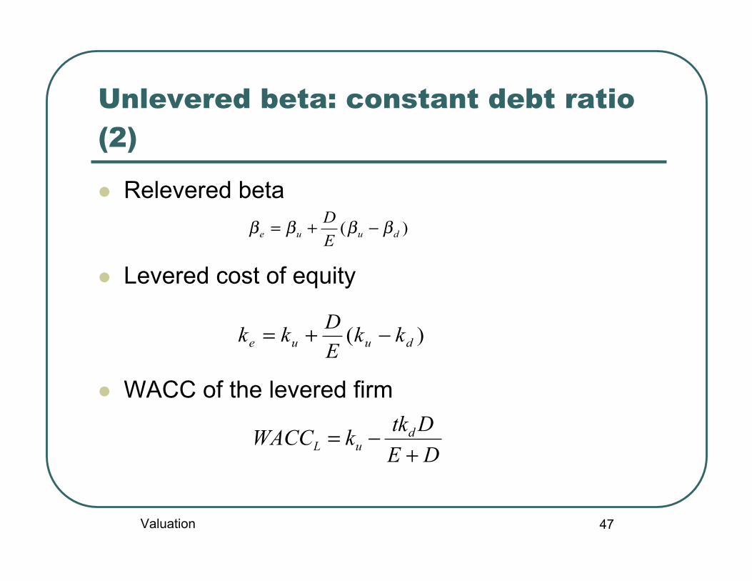
47

Unlevered beta: constant debt ratio(2)

Relevered beta

Levered cost of equity

WACC of the levered firm

)( duue ED ββββ −+=

)( duue kkEDkk −+=

DEDtkkWACC d

uL +−=

Valuation

Constant leverage ratio:example

Redo the previous exercise assumingthat the comparable firm is going tomaintain the current debt ratio in thefuture

48Valuation

49

IV. Estimating residual value Method 1

Method 2

Sincethese two methods are equivalent.

Since the reinvestment rate in the residual period may be differentfrom that in the explicit forecast period, FCFT+1 may not equalFCFT*(1+g)

Method 1 automatically takes this into account.

gWACCRONICgNOPLATRV T

T −−= + )/1(1

gWACCFCFRV T

T −= +1

)/1(*)1(* 111 RONICgNOPLATIRNOPLATFCF TTT −=−= +++

Valuation

50

Residual value: example

FCFT = 100, NOPLATT = 200 From year T+1 on, g = 5%, RONIC=

12% WACC = 10%

Valuation

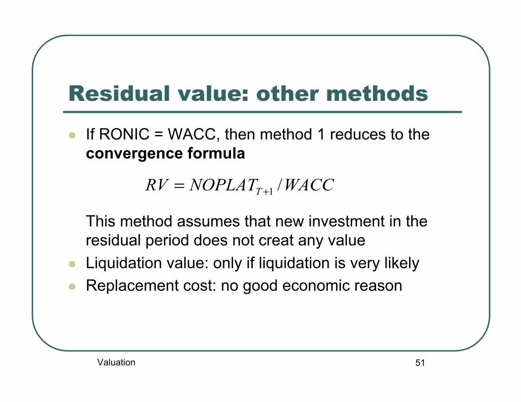
51

Residual value: other methods

If RONIC = WACC, then method 1 reduces to theconvergence formula

This method assumes that new investment in theresidual period does not creat any value

Liquidation value: only if liquidation is very likely Replacement cost: no good economic reason

WACCNOPLATRV T /1+=

Valuation

52

Other DCF valuation model

Capital cash flow valuation model Adjusted present value model Economic-profit-based valuation model Discount dividend model

Valuation

53

Capital cash flow valuationmodel

CCF = FCF + interest tax shield Firm value is derived by discounting the CCF using

unlevered cost of equity Given that interest tax shield are discounted using

unlevered cost of equity, it follows that unleveredcost of equity equals pretax WACC.

Advantage: no need to adjust discount rate forchanges in financial structure.

Valuation

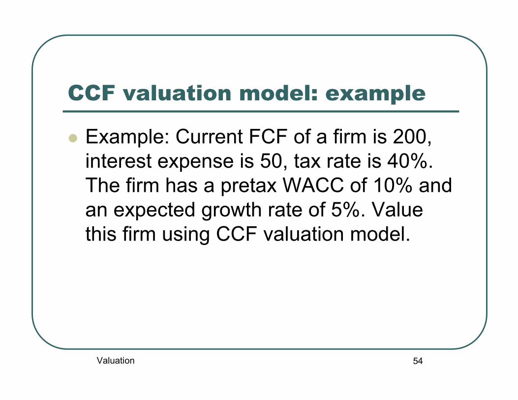
54

CCF valuation model: example

Example: Current FCF of a firm is 200,interest expense is 50, tax rate is 40%.The firm has a pretax WACC of 10% andan expected growth rate of 5%. Valuethis firm using CCF valuation model.

Valuation

55

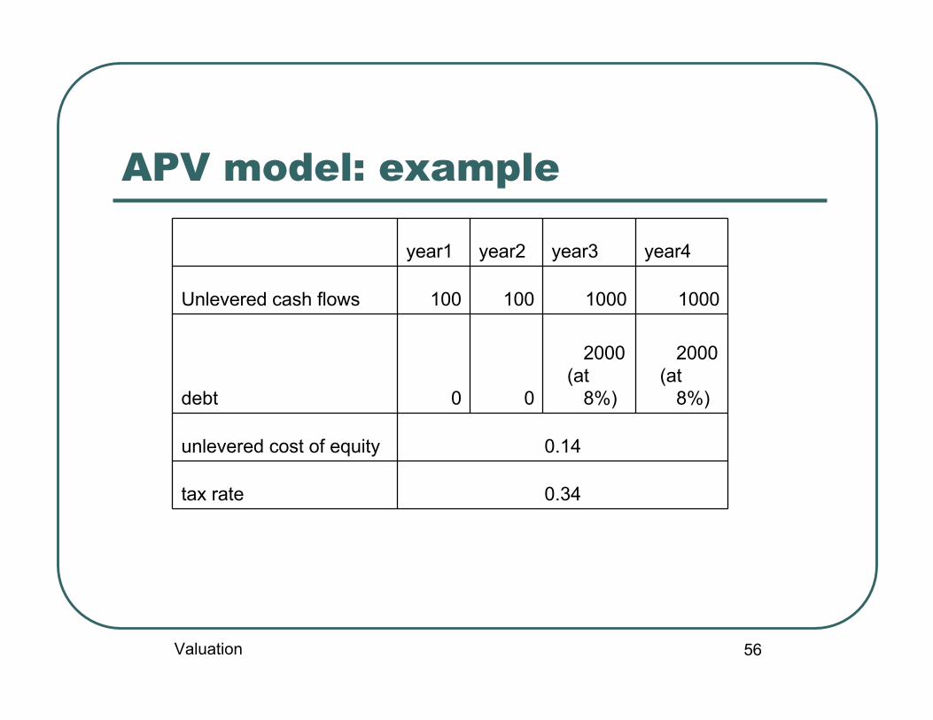
Adjusted present value model Valuation by components approach:

where VU is the expected FCF discounted using unleveredcost of equity, VTS is the present value of interest tax shields

Possible discount rates for interest tax shields:• Pretax cost of debt: varying or risky debt• Unlevered cost of equity: costant debt ratio (in this case, APV

model is equivalent to CCF valuation model) Advantage:

• No need to adjust discount rate for changes in capital structure• Can easily be combined with a variety of valuation models

TSUL VVV +=

Valuation

56

APV model: example

year1 year2 year3 year4

Unlevered cash flows 100 100 1000 1000

debt 0 0

2000 (at

8%)

2000 (at

8%)

unlevered cost of equity 0.14

tax rate 0.34

Valuation

57

Economic-profit-based valuationmodel

Economic profit (or Economic Value Added) = Invested capital * (ROIC-WACC) = NOPLAT – invested capital * WACC

Firm value and economic profit

Important message: a project creates value forshareholders iff its return is higher than its cost of capital

∑∞

= ++=

100 )1(

)(t

tt

WACCprofitEconomicEcapitalInvestedV

Valuation

58

Discount dividend model General model

where DPS is dividend per share, ke = cost ofequity

Gordon growth model: for stocks with a stablegrowth rate

where E(DPS1) is expected dividend nextperiod, g is growth rate in dividends forever

∑∞

= +=

10 )1(

)(t

te

t

kDPSEP

gkDPSEPe −

= )( 10

Valuation

59

Gordon growth model

Works best for companies• in stable growth• in stable leverage• pays out dividend regularly

Limitations• Extremely sensitive to the input for growth

rate• Extremely simple growth pattern

Valuation

60

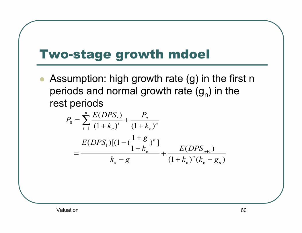
Two-stage growth mdoel

Assumption: high growth rate (g) in the first nperiods and normal growth rate (gn) in therest periods

)()1()(

])11(1)[((

)1()1()(

11

10

nen

e

n

e

n

e

ne

nn

tt

e

t

gkkDPSE

gkkgDPSE

kP

kDPSEP

−++

−++−

=

++

+=

+

=∑

Valuation

2. Relative valuation

62

How does it work?

In relative valuation, you try to figure out thevalue of the firms being analyzed by looking atthe market values of similar or comparablefirms.

Steps in relative valuation• Identify comparable firms• Calculate the „multiples“• Compare the multiples and control for factors that

might affect the multiples Implicit assumption: market is on average right

Valuation

63

Most popular multiples Earnings multiples

• Price/earnings ratio and variants• Value/EBITDA• Value/FCF

Book value multiples• Price/book value (PBV, or market-to-book equity)• Value/book value• Value/replacement cost (Tobin‘s Q)

Revenues multiples• Price/sales• Value/sales

Valuation

64

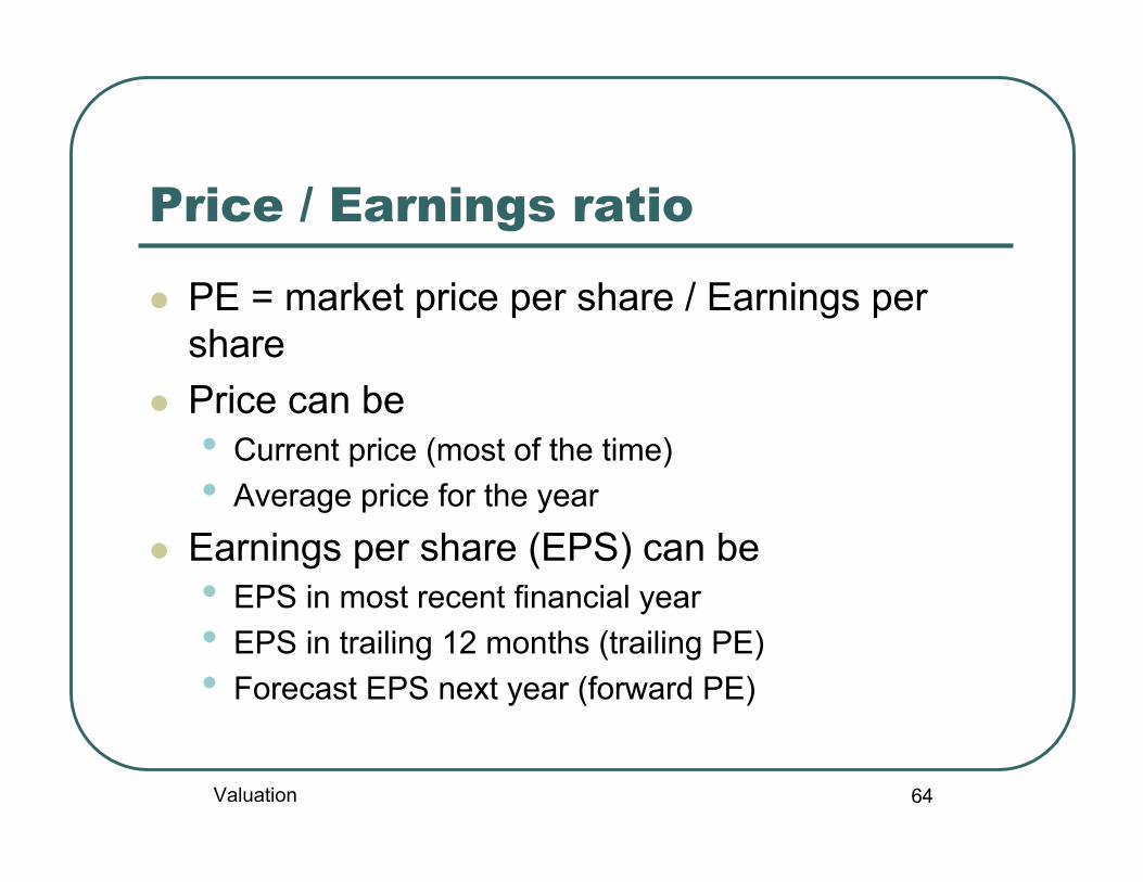
Price / Earnings ratio

PE = market price per share / Earnings pershare

Price can be• Current price (most of the time)• Average price for the year

Earnings per share (EPS) can be• EPS in most recent financial year• EPS in trailing 12 months (trailing PE)• Forecast EPS next year (forward PE)

Valuation

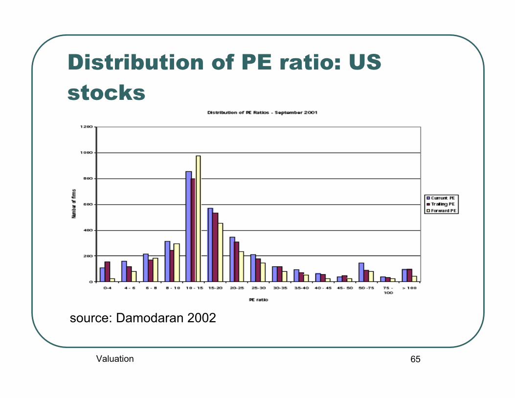
65

Distribution of PE ratio: USstocks

source: Damodaran 2002

Valuation

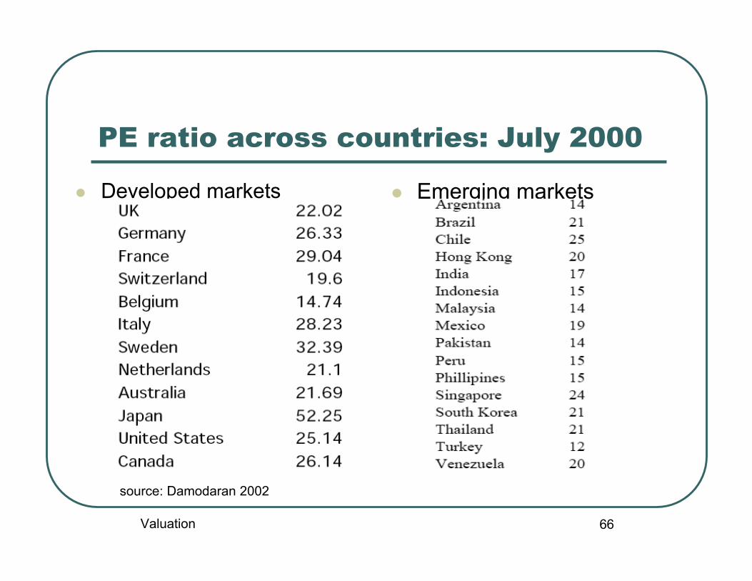
66

PE ratio across countries: July 2000

Developed markets

source: Damodaran 2002

Emerging markets

Valuation

67

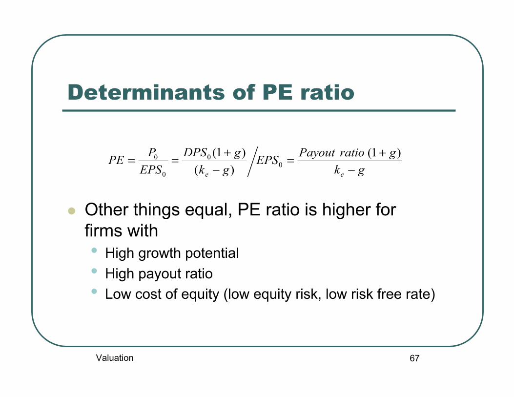
Determinants of PE ratio

Other things equal, PE ratio is higher forfirms with• High growth potential• High payout ratio• Low cost of equity (low equity risk, low risk free rate)

gkgratioPayoutEPS

gkgDPS

EPSPPE

ee −+=

−+== )1()()1(

00

0

0

Valuation

68

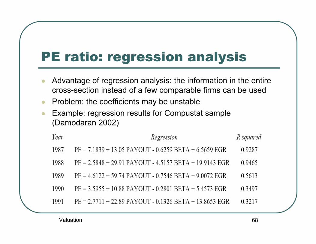
PE ratio: regression analysis Advantage of regression analysis: the informatíon in the entire

cross-section instead of a few comparable firms can be used Problem: the coefficients may be unstable Example: regression results for Compustat sample

(Damodaran 2002)

Valuation

69

PEG ratio PEG = PE / Expected growth rate in earnings A simple way to control for the influence of growth

rate on PE ratio But not completely neutralize it since PE is not a

linear function of expected growth rate

No standard time frame for measuring expectedgrowth rate

)()1(

gkggratioPayoutPEG

e −+=

Valuation

70

Value multiples V / EBITDA = (E + D) / EBITDA V / FCF = (E + D) / FCF FCF = EBIT (1-t) – (CAP EX – D&A) - ∆ working capital

= (EBITDA – D&A)(1-t) - (CAP EX – D&A) - ∆workingcapital

= EBITDA(1-t) + t (D&A) – CAP EX - ∆working capital

Advantages• Less firms with negative EBITDA than firms with

negative earnings• not influenced by difference in depreciation schemes• Not influenced by differences in capital structure

Valuation

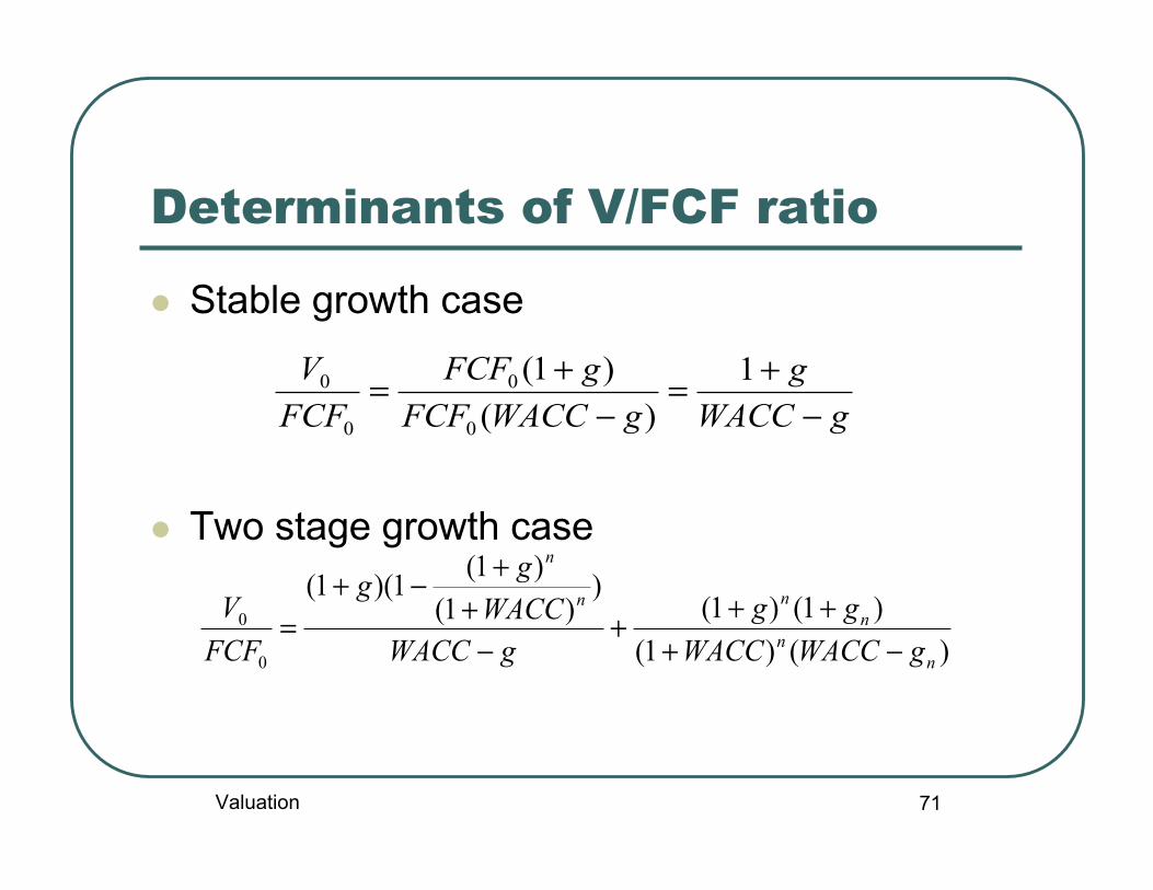
71

Determinants of V/FCF ratio

Stable growth case

Two stage growth case

gWACCg

gWACCFCFgFCF

FCFV

−+=

−+= 1

)()1(

0

0

0

0

)()1()1()1(

))1(

)1(1)(1(

0

0

nn

nnn

n

gWACCWACCgg

gWACCWACCgg

FCFV

−++++

−+

+−+=

Valuation

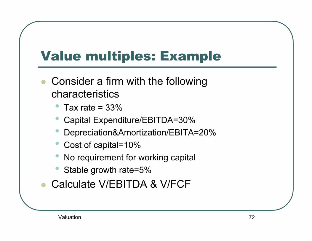
72

Value multiples: Example

Consider a firm with the followingcharacteristics• Tax rate = 33%• Capital Expenditure/EBITDA=30%• Depreciation&Amortization/EBITA=20%• Cost of capital=10%• No requirement for working capital• Stable growth rate=5%

Calculate V/EBITDA & V/FCF

Valuation

73

Value multiples: solution

Valuation

74

Price-to-book ratio

Price-to-book ratio (market-to-book ratio)=market value of equity / book value of equity

For a stable growth firm

Since g=(1-Payout ratio)*ROE, we can further derive

)(*

)(* 1

0

1

0

0

gkratioPayoutROE

gkBVratioPayoutEarnings

BVPPBV

ee −=

−==

gkgROEPBV

e −−=

Valuation

75

PBV and ROE: S&P 500 (Damodaran2002)

Valuation

76

Value-to-book ratio

Definition

For stable growth firm

debtofvaluebookequityofvaluebookdebtofvaluemarketequityofvaluemarket

valueBookValue

++=

gWACCgROIC

gWACCBVROICgtEBIT

gWACCBVFCF

BVV

−−=

−−−=

−=

)()/1)(1(

)( 0

1

0

1

0

0

Valuation

77

Value-to-book ratio: example

Example: Consider a stable growth firmwith the following characteristics:ROIC=12%, WACC=10%, g=5%.Estimate its Value-to-book ratio.

Valuation

78

Tobin‘s Q ratio Definition

If Tobin‘s Q is smaller than 1, then a firm destroysvalue; if it is bigger than 1, then it creates value

Advantage: replacement costs provide a moreupdated measure of asset value than do bookvalues

Disadvantage: replacement costs are hard toestimate

placeinassetsoftplacementplaceinassetsofvalueMarketQsTobin

cosRe' =

Valuation

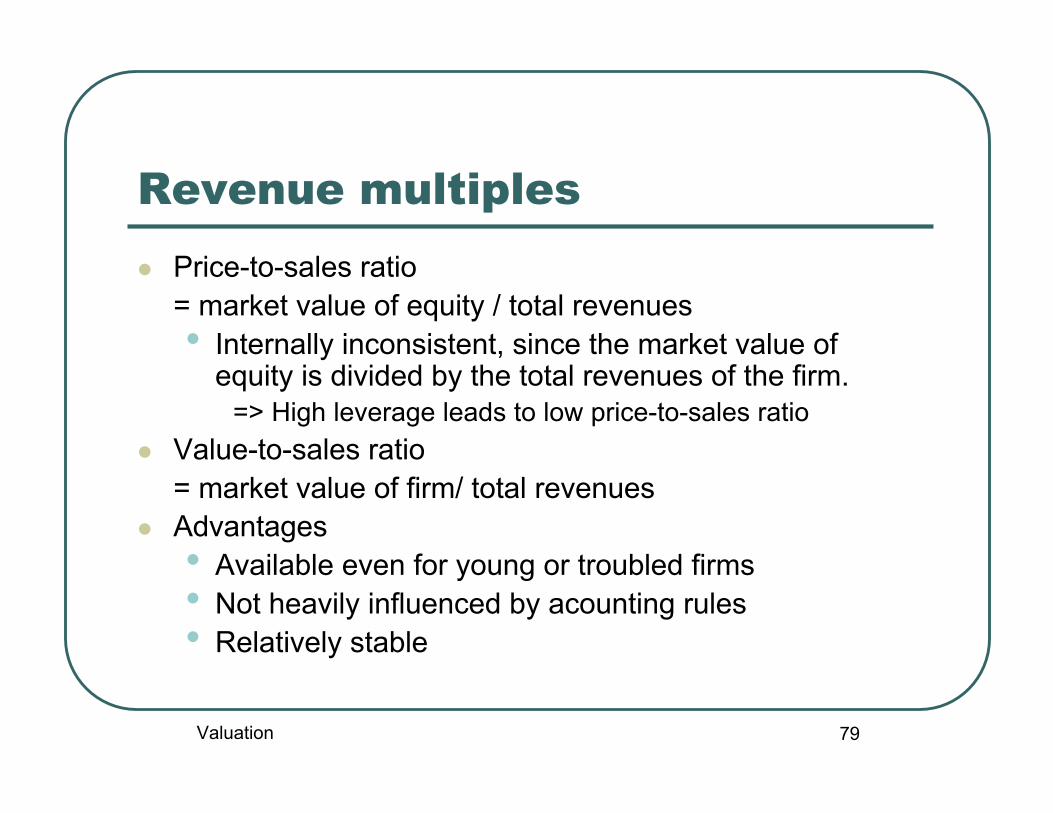
79

Revenue multiples Price-to-sales ratio

= market value of equity / total revenues• Internally inconsistent, since the market value of

equity is divided by the total revenues of the firm. => High leverage leads to low price-to-sales ratio Value-to-sales ratio

= market value of firm/ total revenues Advantages

• Available even for young or troubled firms• Not heavily influenced by acounting rules• Relatively stable

Valuation

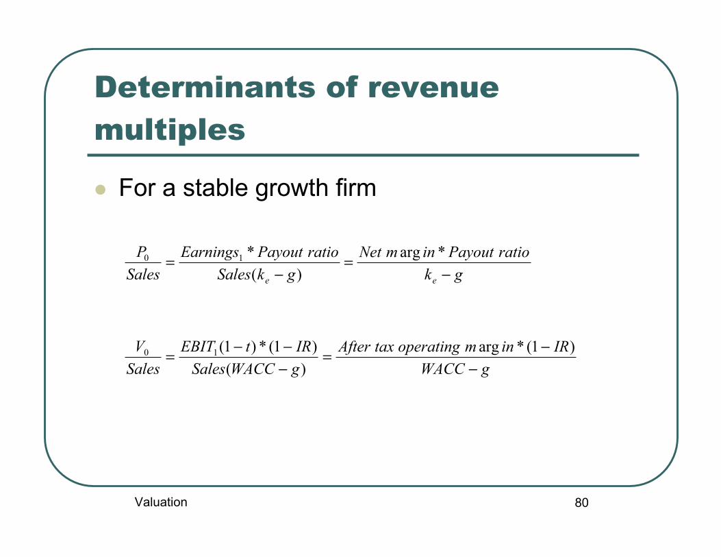
80

Determinants of revenuemultiples

For a stable growth firm

gWACCIRinmoperatingtaxAfter

gWACCSalesIRtEBIT

SalesV

gkratioPayoutinmNet

gkSalesratioPayoutEarnings

SalesP

ee

−−=

−−−=

−=

−=

)1(*arg)()1(*)1(

*arg)(

*

10

10

Valuation

81

Choosing between multiples

There are many potentially useful multiples Which ones to use in valuation?

• Use a simply average of valuations obtained usingdifferent multiples

• Use a weighted average of valuations obtained usingdifferent multiples

• Rely entirely on one of the multiples• Most relevent one• Most accurately estimated one

Valuation

82

Choosing the comparison firms

Three possible choices• A few very similar firms• All firms in the same sector• All firms in the market

Regression analysis is necessary if youchoose the second or third approach

It is recommended to check whether the firm isover or under valued at both the sector andmarket level.

Valuation

3. Real options approachto valuation

84

Managerial flexibility (strategicoptions)

Managers react to changes in economicenvironment

DCF valuation and relative valuation do notexplicitly account for this.

Real options theory provides an usefulframework to quantify the value of flexibility.

This approach is particularly relevant for thevaluation of individual businesses and projects.

Valuation

85

Strategic options: examples

Option to postpone a project Option to abondon a project Option to temporarily shut down a

project Option to expand a project Option to downsize a project Option to change input or output factors

.....Valuation

86

Certainty equivalent method Option pricing is based on the Certainty Equivalent Method

as opposed to the Risk-Adjusted Discount Rate Method. Instead of discounting the expected cash flowes using a

risk-adjusted discount rate, the certainty equivalentmethod discounts the certainty equivalent of futureuncertain cash flows at the risk-free rate.

The certainty equivalent of some uncertain payoff is definedas a sure amount of payoff that is considered to be asvaluable as the uncertain payoff.

This alternative method can be very useful even in theabsence of strategic options.

∑∞

= +=

1 )1()(

tt

f

t

rCFCEQV

Valuation

87

Obtaining certainty equivalents

How can we obtaint certaintyequivalents?• By looking at prices in the forward or futues

market (when forward or futures marketexists)

• Expected value minus dollar value of riskpremium (when risk premium and riskexposure are known)

• Expected value under the risk-neutralprobabilty (when markets are complete)

Valuation

88

Example: two-period gold mine

period1 2

output1000 1000

priceS1 S2

revenue1000S1 1000S2

Costs300 300

NCF 1000S-300 1000S2-300

Valuation

89

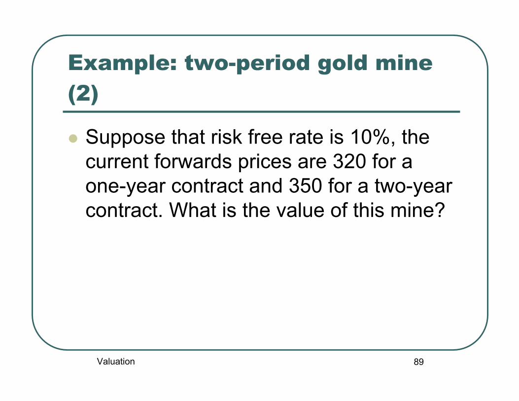
Example: two-period gold mine(2)

Suppose that risk free rate is 10%, thecurrent forwards prices are 320 for aone-year contract and 350 for a two-yearcontract. What is the value of this mine?

Valuation

90

Option pricing methods

Binomial model Black-Scholes formula Monte Carlo simulation

Valuation

91

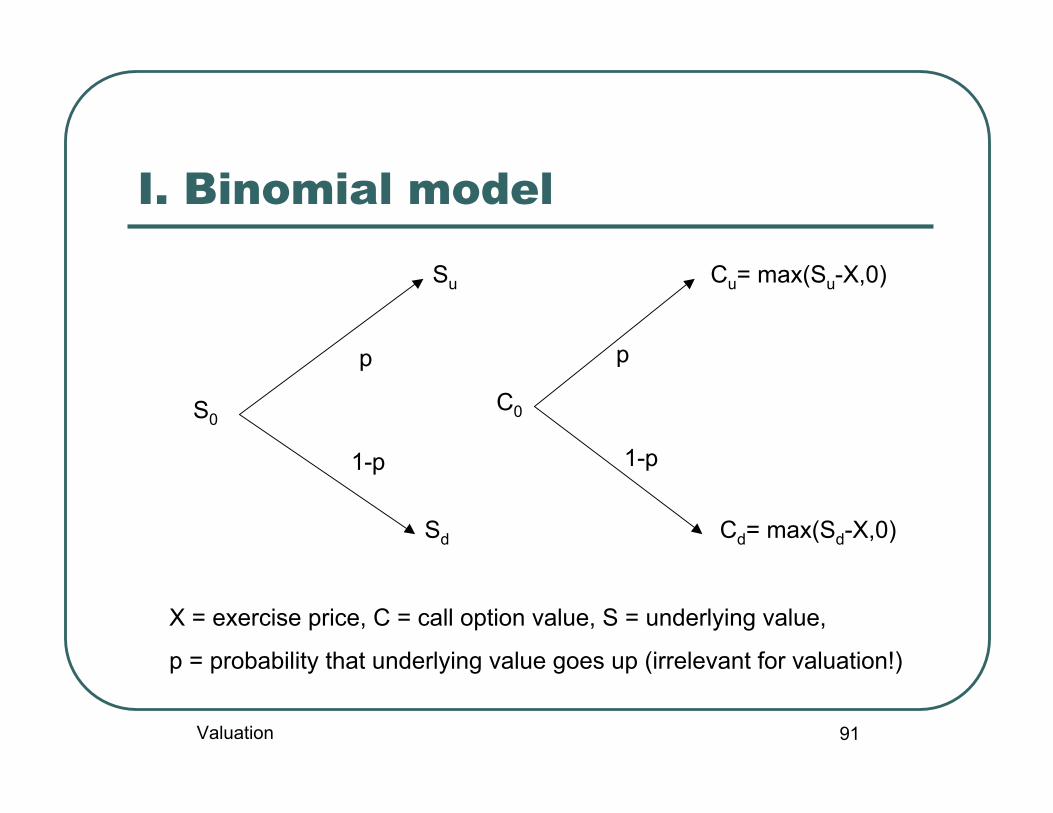
I. Binomial model

S0

Su

Sd

p

1-p

C0

Cu= max(Su-X,0)

Cd= max(Sd-X,0)

X = exercise price, C = call option value, S = underlying value,

p = probability that underlying value goes up (irrelevant for valuation!)

p

1-p

Valuation

92

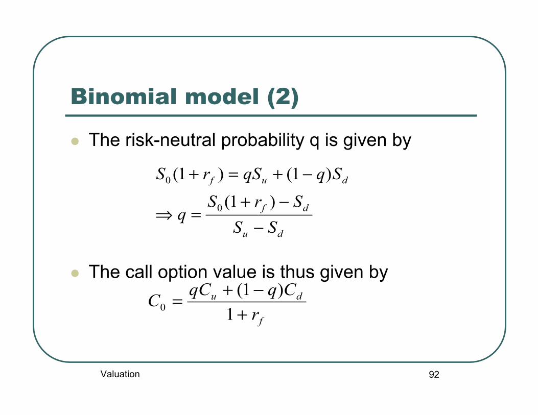
Binomial model (2)

The risk-neutral probability q is given by

The call option value is thus given by

du

df

duf

SSSrS

q

SqqSrS

−−+

=⇒

−+=+

)1()1()1(

0

0

f

du

rCqqCC

+−+=

1)1(

0

Valuation

93

II. Black-Scholes formula For European call and put, Black and Scholes (1973) derive the

following formula

S = underlying price, K = Exercise price, _ = annualized volatility of theunderlying, T = time to maturity, rf = continuously-compounded risk-free rate,N(.) = cumulative standard normal distribution

TddT

TrXS

d

dSNdNXeP

dNXedSNC

f

Tr

Tr

f

f

σσ

σ

−=

++=

−−−=

−=−

−

12

2

1

12

21

)21(ln

)()(

)()(

Valuation

94

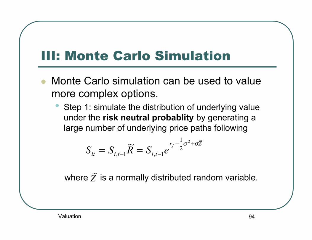
III: Monte Carlo Simulation

Monte Carlo simulation can be used to valuemore complex options.• Step 1: simulate the distribution of underlying value

under the risk neutral probablity by generating alarge number of underlying price paths following

where is a normally distributed random variable.

Zr

titiitfeSRSS

~21

1,1,

2~ σσ +−

−− ==

Z~

Valuation

95

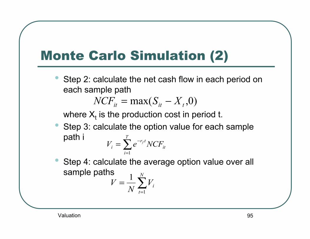
Monte Carlo Simulation (2)• Step 2: calculate the net cash flow in each period on

each sample path

where Xt is the production cost in period t.• Step 3: calculate the option value for each sample

path i

• Step 4: calculate the average option value over allsample paths

∑=

−=T

iit

tri NCFeV f

1

∑=

=N

tiVN

V1

1

)0,max( titit XSNCF −=

Valuation

96

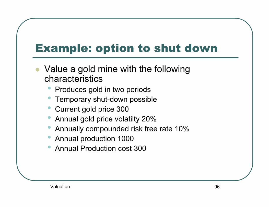
Example: option to shut down

Value a gold mine with the followingcharacteristics• Produces gold in two periods• Temporary shut-down possible• Current gold price 300• Annual gold price volatilty 20%• Annually compounded risk free rate 10%• Annual production 1000• Annual Production cost 300

Valuation

97

Solution: Binomial model

8187.0,2214.1 ==== − tt edeu σσ

S

Su

Sd

Suu

Sud,Sdu

Sdd

Valuation

98

Solution: Binomial model (2)

f

du

f

dduddd

f

uduuuu

f

rVqqVV

rVqqVSV

rVqqVSV

dudr

q

+−+=

+−++−=

+−++−=

−−+

=

1)1(

1)1()0,300max(

1)1()0,300max(

1

0

Valuation

99

Solution: Black-Scholes

tddt

trd

dNdNdNdN

tt

ft

σσ

σ

−=

++=

+

=

=+=

12

2

1

222*0.0953-

21

120.0953-

11

f

)5.0()300/300ln()](300e-)( 300[1000

)](300e-)( 1000[300 V0.095310%)ln(1 r

Valuation

100

Solution: Monte Carlo simulation

Function RAND() generates a random realization of a randomvariable uniformly distributed over the interval [0,1].

NORMSINV(U) generates a random realization of a randomvariable following a standard normal distribution.

()~)~(~

~

~

~21

1,

2

RANDUUNORMSINVZ

eR

RSS

Zr

tiit

f

=

=

=

=

+−

−

σσ

Valuation

101

Monte Carlo simulation: a samplepath

period t=1 t=2U 0.2679 0.7208Z -0.6193 0.5853R 0.9526 1.2121S 285.78 346.40Production cost 300 300NCF 0 46.40PV 0 38350.41V 38350.41

Valuation

102

Option to delay: example Panel A: Invest now

Panel B: wait one year and invest only in good state

-100

10 15 15 per year for ever

good

10 2.5 2.5 per year for ever

bad

0

-100 15 15 per year for ever

good

0 0 0 per year for ever

bad

Valuation

103

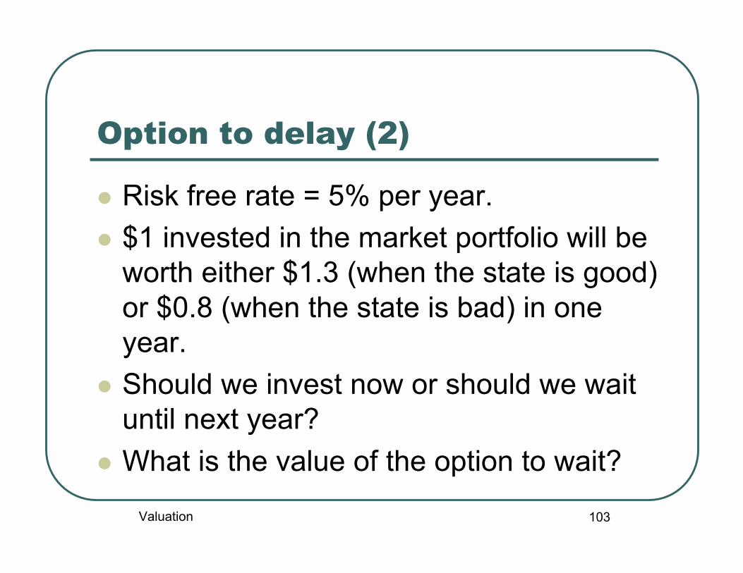
Option to delay (2)

Risk free rate = 5% per year. $1 invested in the market portfolio will be

worth either $1.3 (when the state is good)or $0.8 (when the state is bad) in oneyear.

Should we invest now or should we waituntil next year?

What is the value of the option to wait?

Valuation

104

Option to delay: solution

Valuation

105

Option to expand: example A project can generate the following CFs:

The firm has the option to double its capacity by investing another 140in year 1 if the economy looks good.

-140

good

bad

200

150

100

Valuation

106

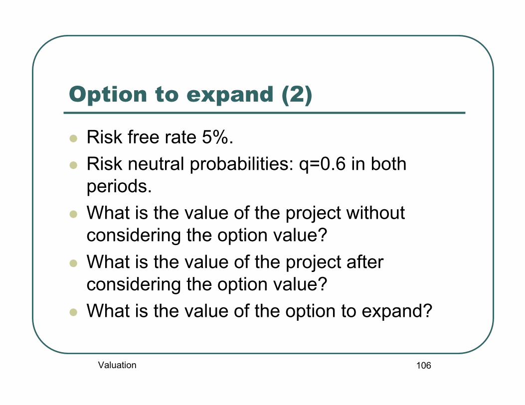
Option to expand (2)

Risk free rate 5%. Risk neutral probabilities: q=0.6 in both

periods. What is the value of the project without

considering the option value? What is the value of the project after

considering the option value? What is the value of the option to expand?

Valuation

107

Option to expand: solution

Valuation