Embed Size (px)
Citation preview
V. Finite Element Method
5.1 Introduction to Finite Element Method
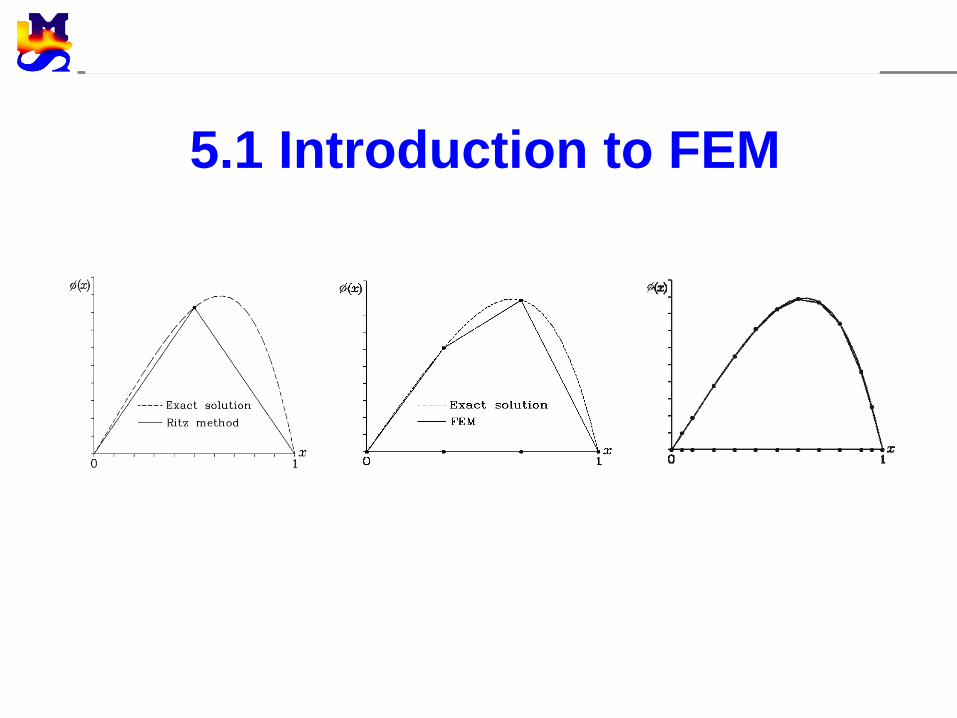
5.1 Introduction to FEM
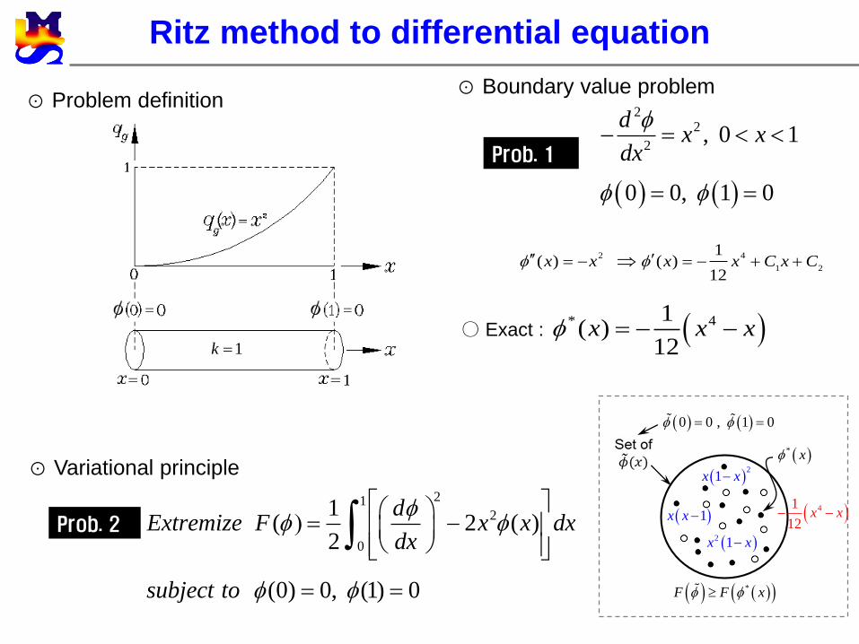
⊙ Boundary value problem⊙ Problem definition
* 41( )
12x x x
⊙ Variational principle
Prob. 1
Prob. 2
1k ○ Exact :
22
2, 0 1
0 0, 1 0
dx x
dx
212
0
1( 2 ( )
2
(0) 0, (1) 0
dExtremize F x x dx
dx
subject to
2 4
1 2
1( ) ( )
12x x x x C x C
Ritz method to differential equation
0 0 , 1 0
* x
*F F x
2
1x x
1x x
2 1x x
41
12x x
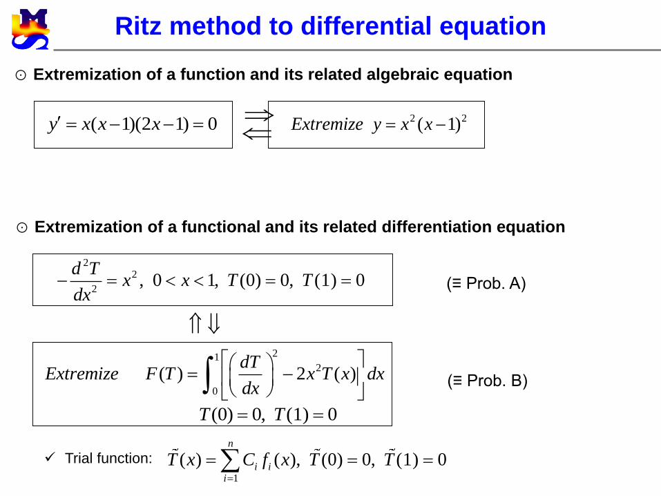
( 1)(2 1) 0y x x x 2 2( 1)Extremize y x x
22
2, 0 1, (0) 0, (1) 0
d Tx x T T
dx
212
0
( ) 2 ( )dT
Extremize F T x T x dxdx
(0) 0, (1) 0T T
Trial function:
1
( ) ( ), (0) 0, (1) 0n
i ii
T x C f x T T
(≡ Prob. A)
(≡ Prob. B)
Ritz method to differential equation
⊙ Extremization of a function and its related algebraic equation
⊙ Extremization of a functional and its related differentiation equation
Ritz method to differential equation
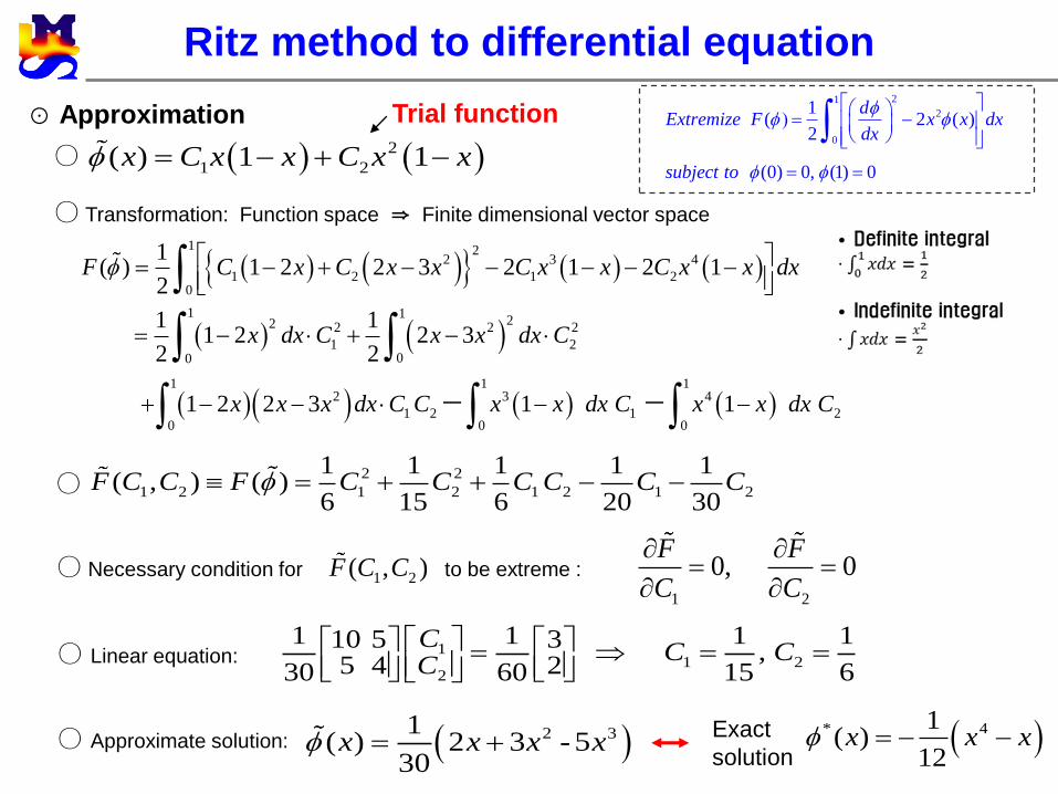
○ Necessary condition for to be extreme :
⊙ Approximation
○ 2
1 2( ) 1 1x C x x C x x
1 2
2 3 4
1 2 1 20
1( ) 1 2 2 3 2 1 2 1
2F C x C x x C x x C x x dx
1 122 2 2 2
1 200
1 11 2 2 3
2 2x dx C x x dx C
1 1 1
2 3 4
1 2 1 20 0 0
1 2 2 3 1 1x x x dx C C x x dx C x x dx C
1 2
0, 0F F
C C
2 2
1 2 1 2 1 2 1 2
1 1 1 1 1( , ) ( )
6 15 6 20 30F C C F C C C C C C ○
○ Linear equation: 11 2
2
1 1 1 110 5 3 ,
5 4 230 60 15 6
CC C
C
2 31( ) 2 3 - 5
30x x x x ○ Approximate solution:
○ Transformation: Function space ⇒ Finite dimensional vector space
* 41( )
12x x x Exact
solution
21
2
0
1( 2 ( )
2
(0) 0, (1) 0
dExtremize F x x dx
dx
subject to
Trial function
1 2( , )F C C
12
0[ ( ) ( ) ( )] 0
(0) 0, (1) 0
( )
(0) 0 (1) 0
where is arbitrary exc
x x x x
ept t
d
h
x
a
an
tx
d
22
20, 0 1
0 0, 1 0
dx x
dx
0 0 , 1 0
* x
2
1x x
1x x
2 1x x
41
12x x
21
2
20( ) 0
0 1 0
dx x dx
dx
11 2
0 0( ) ( ) ( ) ( ) ( ) 0
(0) (1) 0
Assume (0) (1) 0
x x x x x x dx
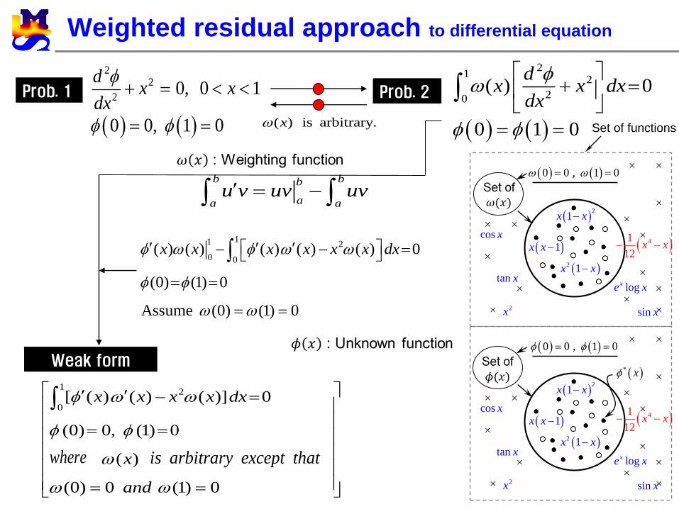
( ) is arbitrary.x
Weak form
sin x
tan x
cos x
logxe x
2x
0 0 , 1 0
2
1x x
1x x
2 1x x
41
12x x
sin x
tan x
cos x
logxe x
2x
b bb
aa au v uv uv
where is arbitrary except that
Weighted residual approach to differential equation
Prob. 1 Prob. 2
Set of functions
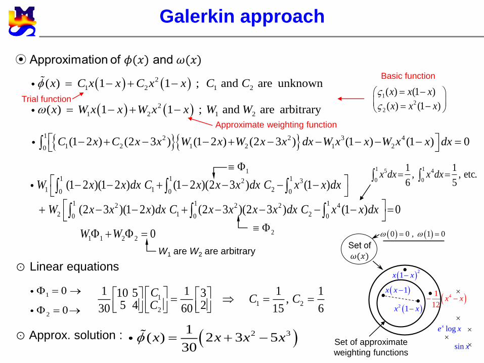
⊙ Linear equations
2 31( ) 2 3 5
30x x x x ⊙ Approx. solution :
2
1 2 1 2( ) 1 1 ; and are unknownx C x x C x x C C
2
1 2 1 2( ) 1 1 ; and are arbitraryx W x x W x x W W
1 2 2 3 4
1 2 1 2 1 20(1 2 ) (2 3 ) (1 2 ) (2 3 ) (1 ) (1 ) 0C x C x x W x W x x dx W x x W x x dx
1 1 12 3
1 1 20 0 0
1 1 12 2 2 4
2 1 20 0 0
(1 2 )(1 2 ) (1 2 )(2 3 ) (1 )
(2 3 )(1 2 ) (2 3 )(2 3 ) (1 ) 0
W x x dx C x x x dx C x x dx
W x x x dx C x x x x dx C x x dx
2
1 15 4
0 0
1 1, , etc.
6 5x dx x dx
1
12
2
( ) (1 )
( ) (1 )
x x x
x x x
1 1 2 2 0W W
W1 are W2 are arbitrary
1x x
2 1x x
41
12x x
sin x
logxe x
0 0 , 1 0
2
1x x
Galerkin approach
11 2
2
1 1 1 110 5 3 ,
5 4 230 60 15 6
CC C
C
1
2
0
0
Trial function
Basic function
Approximate weighting function
Set of approximate
weighting functions
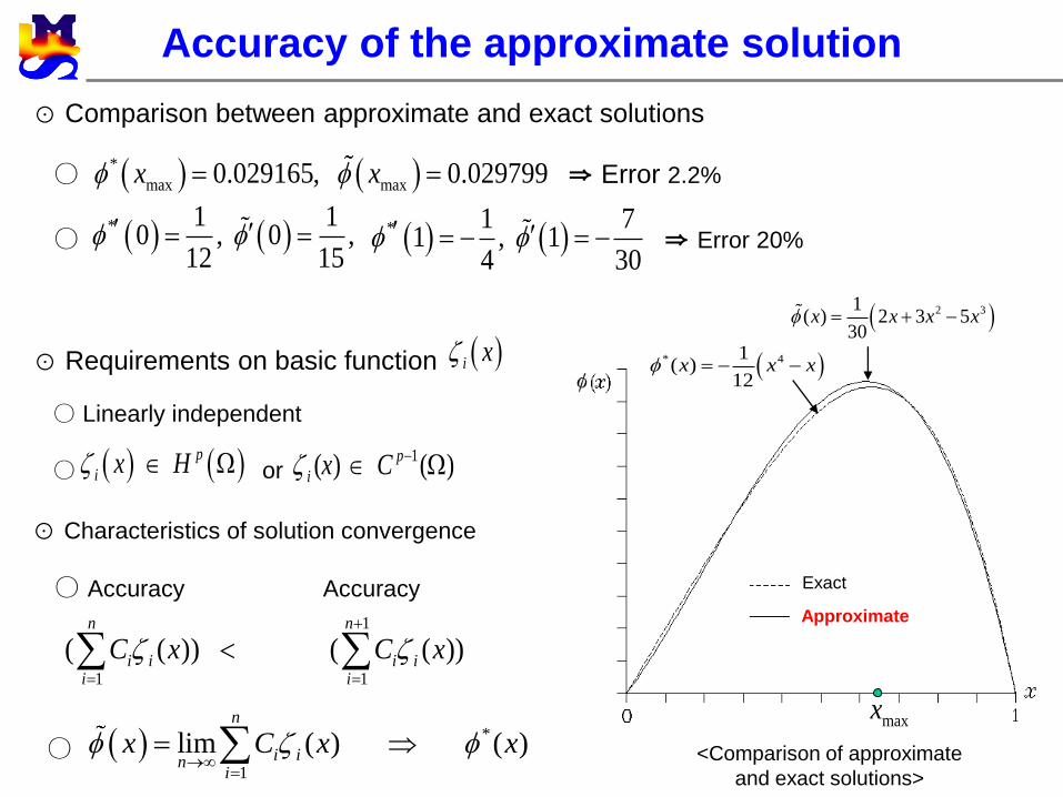
⊙ Characteristics of solution convergence
○ Accuracy Accuracy
○
⊙ Requirements on basic function
○ Linearly independent
○ or
1
1 1
( ( )) ( ( ))n n
i i i ii i
C x C x
*
1
lim ( ) ( )n
i ini
x C x x
i x
p
i x H 1( ) ( )p
i x C
<Comparison of approximate
and exact solutions>
○ ⇒ Error 2.2%
○ ⇒ Error 20% * 1 10 , 0 ,
12 15 * 1 7
1 , 14 30
*
max max0.029165, 0.029799 x x
⊙ Comparison between approximate and exact solutions
Exact
Approximate
2 31( ) 2 3 5
30x x x x
* 41( )
12x x x
maxx
Accuracy of the approximate solution
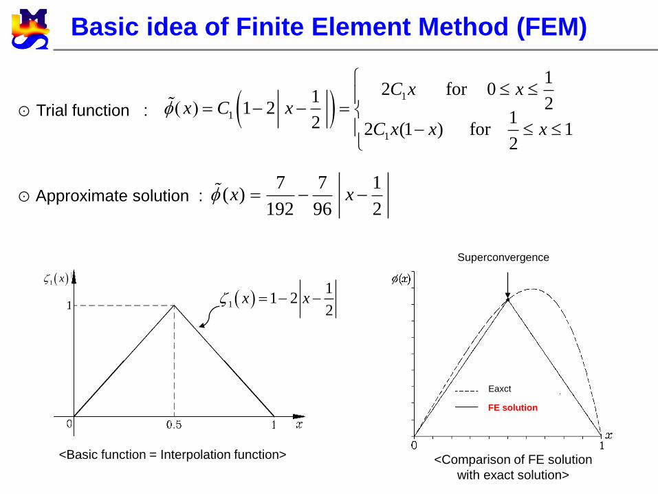
<Basic function = Interpolation function>
⊙ Trial function : 1
1
1
12 for 01 21 2
12 2 (1 ) for 12
C x xx C x
C x x x
7 7 1( )
192 96 2x x ⊙ Approximate solution :
Eaxct
FE solution
<Comparison of FE solution
with exact solution>
1
11 2
2x x
1 x
Superconvergence
Basic idea of Finite Element Method (FEM)
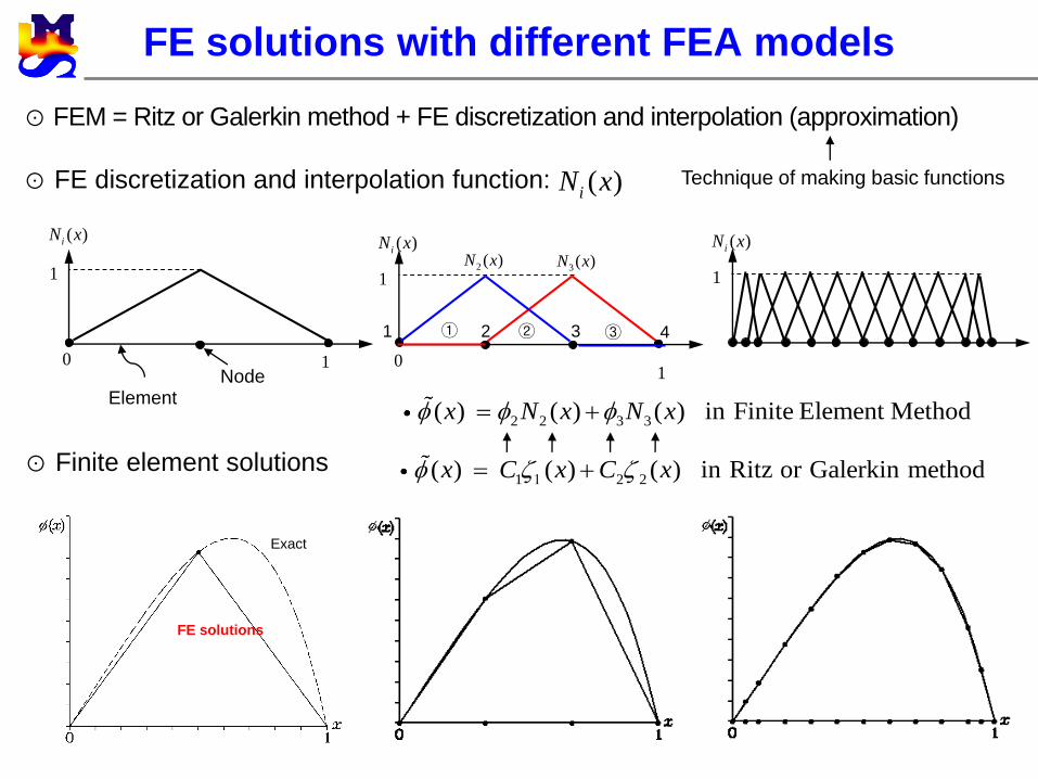
Exact
FE solutions
⊙ FEM = Ritz or Galerkin method + FE discretization and interpolation (approximation)
⊙ FE discretization and interpolation function: ( )iN x
⊙ Finite element solutions
3( )N x
1 2 3 4① ② ③
2 ( )N x
2 2 3 3( ) ( ) ( ) in Finite Element Methodx N x N x
1 2 2( ) ( ) ( ) in Ritz or Galerkin methodx C x C x
Technique of making basic functions
FE solutions with different FEA models
( )iN x( )iN x
1 1
( )iN x
1
0 1 01
ElementNode
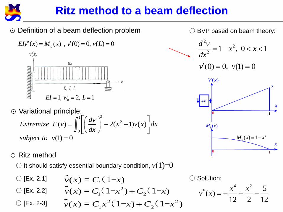
⊙ Definition of a beam deflection problem
4 2* 5( )
12 2 12
x xv x
○ Solution:
22
21 , 0 1
dx x
dx
(0) 0, (1) 0v v
⊙ Variational principle:21
2
0
( ) 2( 1) ( )dv
Extremize F v x v x dxdx
(1) 0subject to v
⊙ Ritz method
○ It should satisfy essential boundary condition, (1)=0 v
○ [Ex. 2.1]1( ) )v x C x = (1-
○ [Ex. 2.2] 2
1 2( ) ) )v x C x C x = (1- (1-
○ [Ex. 2-3] 2 2
1 2( ) ) )v x C x x C x= (1- (1-
○ BVP based on beam theory:
V
( )V x
x
0 1
2
x
0 1
1
( )bM x
( ) ( )bEIv x M x , (0) 0, ( ) 0v v L
2( ) 1bM x x
Ritz method to a beam deflection
01, 2, 1EI w L
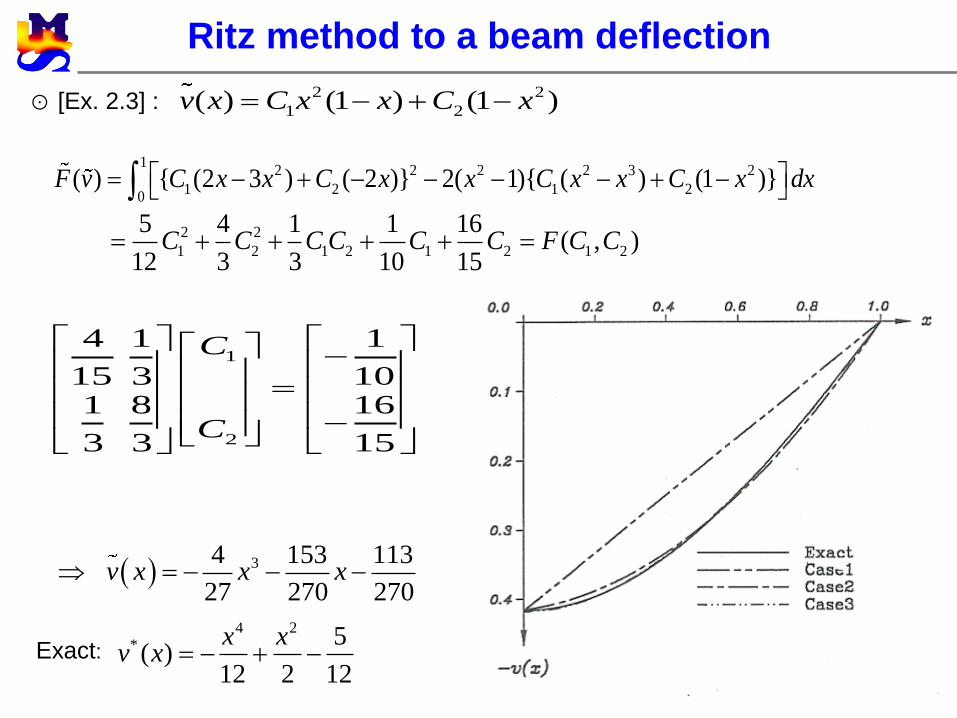
⊙ [Ex. 2.3] :2 2
1 2( ) (1 ) (1 )v x C x x C x
12 2 2 2 3 2
1 2 1 20
( ) { (2 3 ) ( 2 )} 2( 1){ ( ) (1 )}F v C x x C x x C x x C x dx 2 2
1 2 1 2 1 2 1 2
5 4 1 1 16( , )
12 3 3 10 15C C C C C C F C C
1
2
4 1 1
15 3 101 8 16
3 3 15
C
C
34 153 113
27 270 270v x x x
4 2* 5( )
12 2 12
x xv x Exact:
Ritz method to a beam deflection
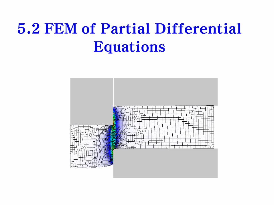
5.2 FEM of Partial Differential
Equations
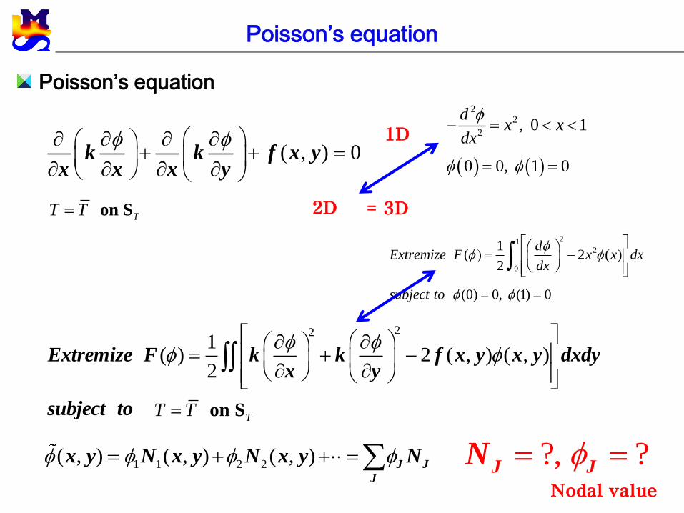
Poisson’s equation
Poisson’s equation
TT T on S
( , ) 0
k k f x yx x x y
22
2, 0 1
0 0, 1 0
dx x
dx
212
0
1( 2 ( )
2
(0) 0, (1) 0
dExtremize F x x dx
dx
subject to
221
( ) 2 ( , ) ( , )2
Extremize F k k f x y x y dxdy
x y
subject toTT T on S
1 1 2 2( , ) ( , ) ( , ) J J
J
x y N x y N x y N ?, ? J J
N
2D
1D
= 3D
Nodal value

Mesh
Mesh system
J
Interpolation function ( , )JN x y
1
1
-1
-1ξ
η
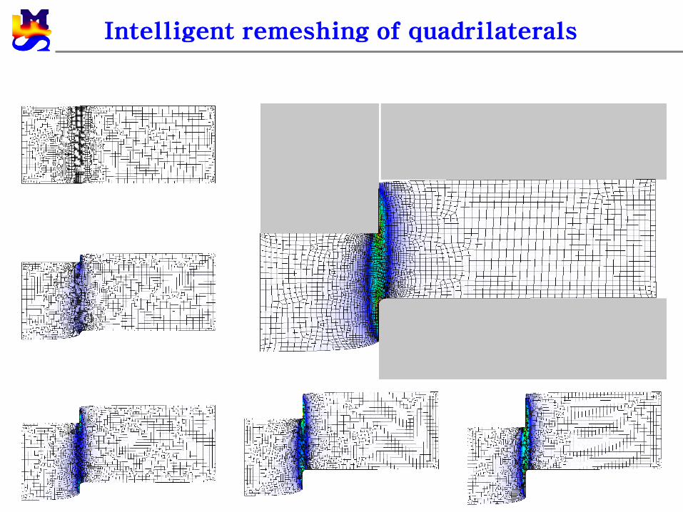
Intelligent remeshing of quadrilaterals
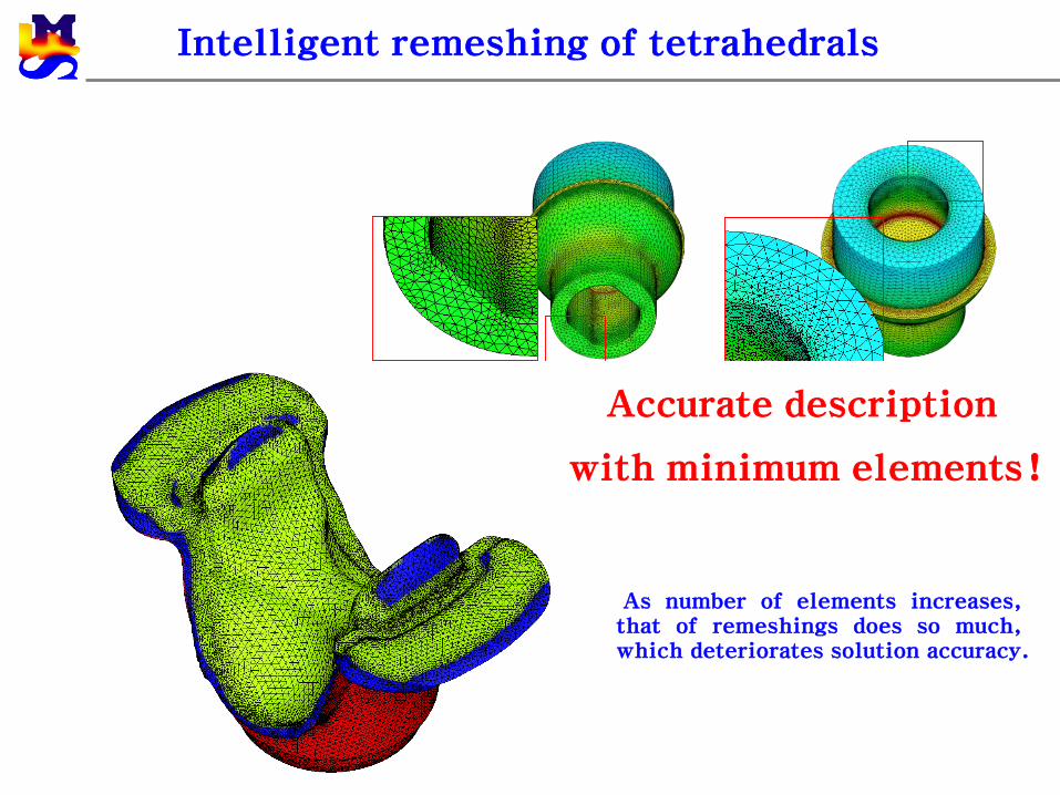
Intelligent remeshing of tetrahedrals
Accurate description
with minimum elements!
As number of elements increases,that of remeshings does so much,which deteriorates solution accuracy.
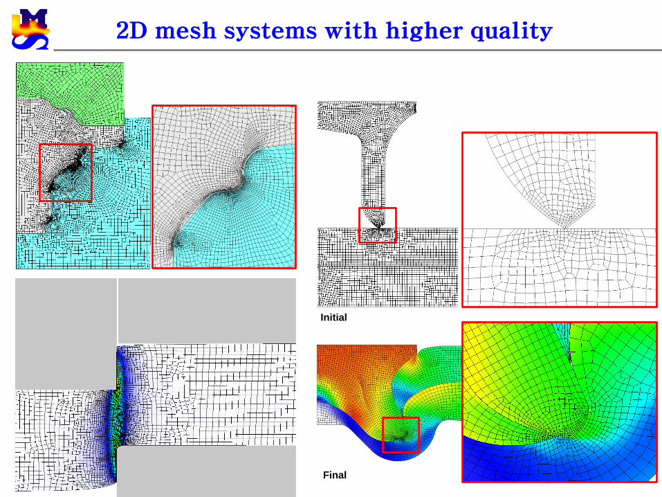
2D mesh systems with higher quality
Initial
Final
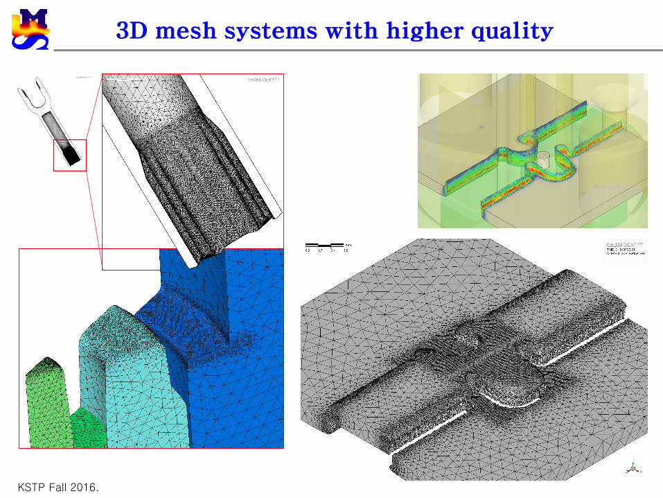
KSTP Fall 2016.
3D mesh systems with higher quality
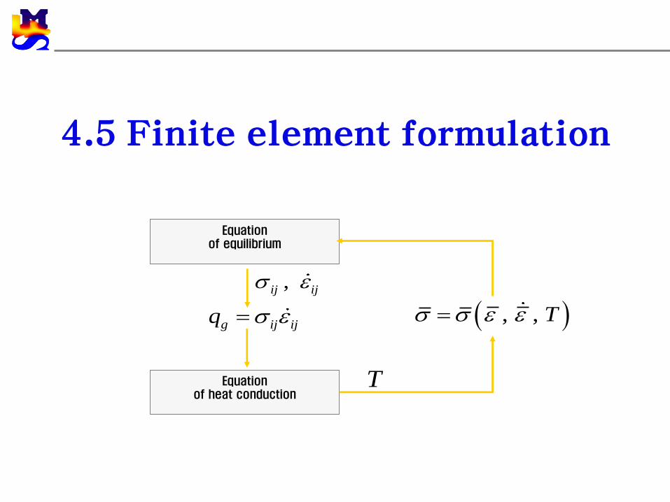
4.5 Finite element formulation
Equation of equilibrium
Equation of heat conduction
T
,ij ij
g ij ijq , , T
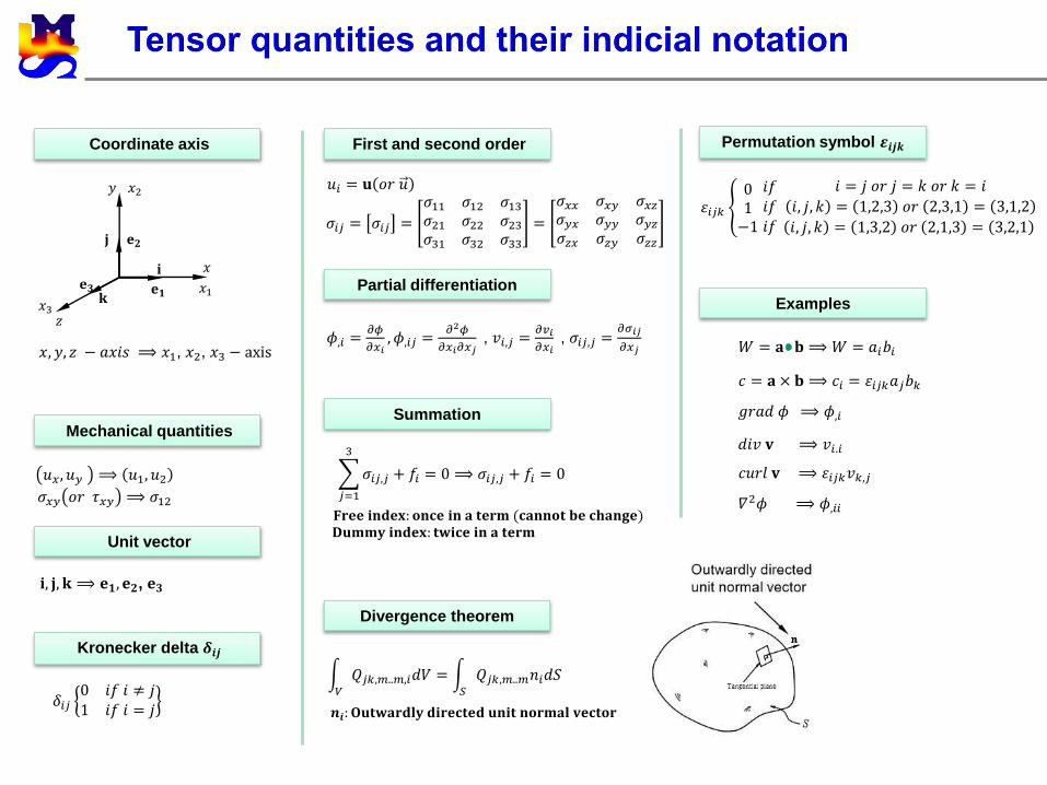
Coordinate axis
𝑦
𝑥
𝑥2
𝑧𝑥3
𝑥1𝐞𝟏
𝐞𝟐
𝐞𝟑
𝐣
𝐢
𝐤
𝑥, 𝑦, 𝑧 − 𝑎𝑥𝑖𝑠 ⟹ 𝑥1, 𝑥2, 𝑥3 − axis
Mechanical quantities
𝑢𝑥, 𝑢𝑦 ⟹ 𝑢1, 𝑢2𝜎𝑥𝑦 𝑜𝑟 𝜏𝑥𝑦 ⟹ 𝜎12
Unit vector
𝐢, 𝐣, 𝐤 ⟹ 𝐞𝟏, 𝐞𝟐, 𝐞𝟑
Kronecker delta 𝜹𝒊𝒋
𝛿𝑖𝑗0 𝑖𝑓 𝑖 ≠ 𝑗1 𝑖𝑓 𝑖 = 𝑗
First and second order
𝑢𝑖 = 𝐮 𝑜𝑟 𝑢
𝜎𝑖𝑗 = 𝜎𝑖𝑗 =
𝜎11 𝜎12 𝜎13𝜎21 𝜎22 𝜎23𝜎31 𝜎32 𝜎33
=
𝜎𝑥𝑥 𝜎𝑥𝑦 𝜎𝑥𝑧𝜎𝑦𝑥 𝜎𝑦𝑦 𝜎𝑦𝑧𝜎𝑧𝑥 𝜎𝑧𝑦 𝜎𝑧𝑧
Partial differentiation
𝜙,𝑖 =𝜕𝜙
𝜕𝑥𝑖, 𝜙,𝑖𝑗 =
𝜕2𝜙
𝜕𝑥𝑖𝜕𝑥𝑗, 𝑣𝑖,𝑗 =
𝜕𝑣𝑖
𝜕𝑥𝑖, 𝜎𝑖𝑗,𝑗 =
𝜕𝜎𝑖𝑗
𝜕𝑥𝑗
Summation
𝑗=1
3
𝜎𝑖𝑗,𝑗 + 𝑓𝑖 = 0 ⟹ 𝜎𝑖𝑗,𝑗 + 𝑓𝑖 = 0
𝐅𝐫𝐞𝐞 𝐢𝐧𝐝𝐞𝐱: 𝐨𝐧𝐜𝐞 𝐢𝐧 𝐚 𝐭𝐞𝐫𝐦 (𝐜𝐚𝐧𝐧𝐨𝐭 𝐛𝐞 𝐜𝐡𝐚𝐧𝐠𝐞)𝐃𝐮𝐦𝐦𝐲 𝐢𝐧𝐝𝐞𝐱: 𝐭𝐰𝐢𝐜𝐞 𝐢𝐧 𝐚 𝐭𝐞𝐫𝐦
Divergence theorem
𝑉
𝑄𝑗𝑘,𝑚..𝑚,𝑖𝑑𝑉 = 𝑆
𝑄𝑗𝑘,𝑚..𝑚𝑛𝑖𝑑𝑆
𝒏𝒊: 𝐎𝐮𝐭𝐰𝐚𝐫𝐝𝐥𝐲 𝐝𝐢𝐫𝐞𝐜𝐭𝐞𝐝 𝐮𝐧𝐢𝐭 𝐧𝐨𝐫𝐦𝐚𝐥 𝐯𝐞𝐜𝐭𝐨𝐫
Permutation symbol 𝜺𝒊𝒋𝒌
휀𝑖𝑗𝑘 01−1
𝑖𝑓𝑖𝑓𝑖𝑓
𝑖 = 𝑗 𝑜𝑟 𝑗 = 𝑘 𝑜𝑟 𝑘 = 𝑖
𝑖, 𝑗, 𝑘 = 1,2,3 𝑜𝑟 2,3,1 = 3,1,2
𝑖, 𝑗, 𝑘 = 1,3,2 𝑜𝑟 2,1,3 = 3,2,1
Examples
𝑐 = 𝐚 × 𝐛 ⟹ 𝑐𝑖 = 휀𝑖𝑗𝑘𝑎𝑗𝑏𝑘
𝑑𝑖𝑣 𝐯 ⟹ 𝑣𝑖.𝑖
𝑔𝑟𝑎𝑑 𝜙 ⟹ 𝜙,𝑖
𝑐𝑢𝑟𝑙 𝐯 ⟹ 휀𝑖𝑗𝑘𝑣𝑘,𝑗
𝛻2𝜙 ⟹ 𝜙,𝑖𝑖
𝑊 = 𝐚 𝐛⟹𝑊 = 𝑎𝑖𝑏𝑖
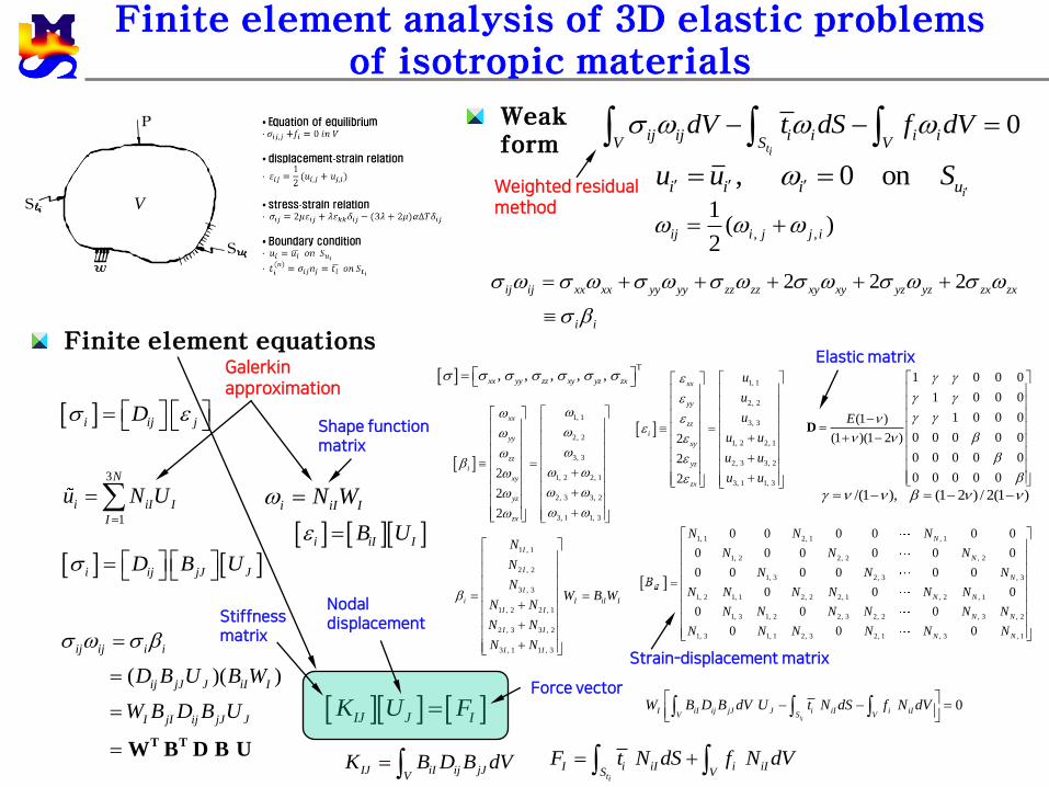
Finite element analysis of 3D elastic problems of isotropic materials
0ti
ij ij i i i iV S V
dV t dS f dV , 0 on
ii i i uu u S
Weak form
S
P
S
VV
2 2 2ij ij xx xx yy yy zz zz xy xy yz yz zx zx
i i
Finite element equations
T
, , , , ,xx yy zz xy yz zx
1, 1
2, 2
3, 3
1, 2 2, 1
2, 3 3, 2
3, 1 1, 3
2
2
2
xx
yy
zz
i
xy
yz
zx
i ij jD
1, 1
2, 2
3, 3
1, 2 2, 1
2, 3 3, 2
3, 1 1, 3
2
2
2
xx
yy
zz
i
xy
yz
zx
u
u
u
u u
u u
u u
1 0 0 0
1 0 0 0
1 0 0 0(1 )
0 0 0 0 0(1 )(1 2 )
0 0 0 0 0
0 0 0 0 0
E
D
/(1 ), (1 2 ) / 2(1 )
3
1
N
i iI I
I
u N U
i iI IB U
1 , 1
2 , 2
3 , 3
1 , 2 2 , 1
2 , 3 3 , 2
3 , 1 1 , 3
I
I
I
i I iI I
I I
I I
I I
N
N
NW B W
N N
N N
N N
i ij jJ JD B U
( )( )
T TW B D B U
ij ij i i
ij jJ J iI I
I jI ij jJ J
D B U B W
W B D B U
0ti
I iI ij jJ J i iI i iIV S V
W B D B dV U t N dS f N dV
IJ J IK U F
IJ iI ij jJV
K B D B dV ti
I i iI i iIS V
F t N dS f N dV
, ,
1( )
2ij i j j i
Galerkinapproximation
Weighted residual method
i iI IN W
Shape function matrix
Stiffness matrix
Force vector
Strain-displacement matrix
Nodal displacement
Elastic matrix
1, 1 2, 1 , 1
1, 2 2, 2 , 2
1, 3 2, 3 , 3
1, 2 1, 1 2, 2 2, 1 , 2 , 1
1, 3 1, 2 2, 3 2, 2 , 3 , 2
1, 3 1, 1 2, 3 2, 1 , 3 , 1
0 0 0 0 0 0
0 0 0 0 0 0
0 0 0 0 0 0
0 0 0
0 0 0
0 0 0
N
N
N
iI
N N
N N
N N
N N N
N N N
N N N
N N N N N N
N N N N N N
N N N N N N
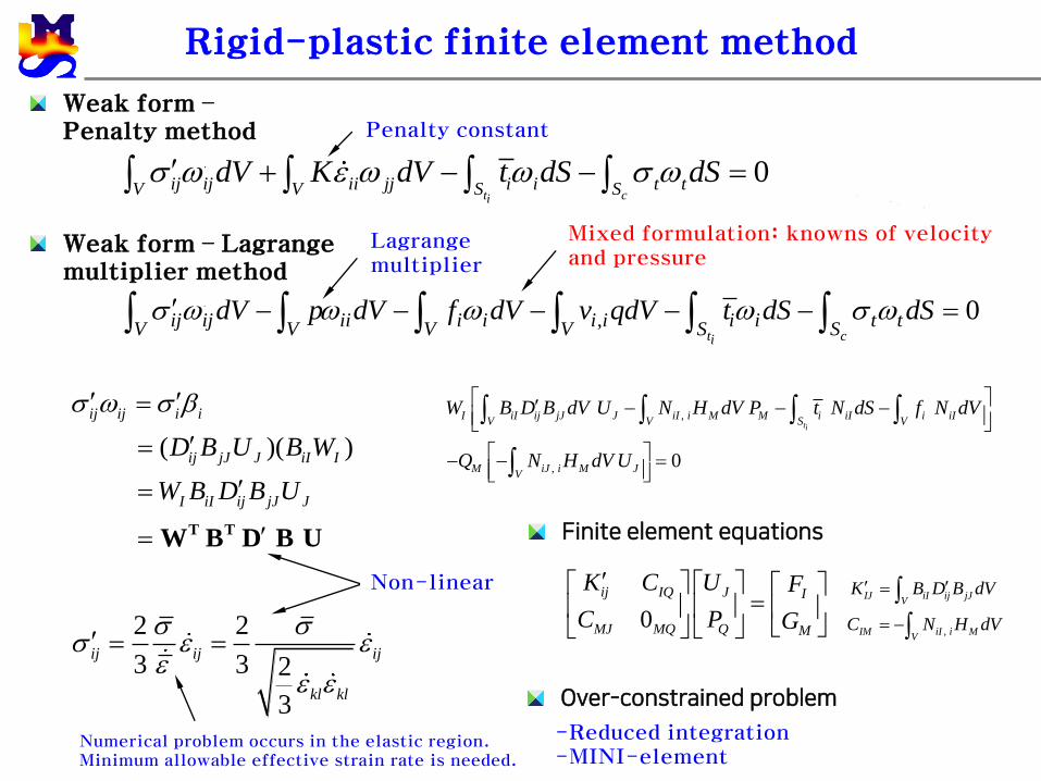
Rigid-plastic finite element method
Mixed formulation: knowns of velocity and pressure
Weak form –Penalty method
Weak form – Lagrange multiplier method
Lagrange multiplier
Penalty constant
( )( )
T TW B D B U
ij ij i i
ij jJ J iI I
I iI ij jJ J
D B U B W
W B D B U
0t ci
ij ij ii jj i i t tV V S SdV K dV t dS dS
, 0t ci
ij ij ii i i i i i i t tV V V V S SdV p dV f dV v qdV t dS dS
,
, 0
ti
I iI ij jJ J iI i M M i iI i iIV V S V
M iJ i M JV
W B D B dV U N H dV P t N dS f N dV
Q N H dV U
2 2
3 3 2
3
ij ij ij
kl kl
Non-linear
0
ij IQ J I
MJ MQ Q M
K C U F
C P G
IJ iI ij jJV
K B D B dV
,IM iI i MV
C N H dV
Numerical problem occurs in the elastic region. Minimum allowable effective strain rate is needed.
Finite element equations
-Reduced integration-MINI-element
Over-constrained problem
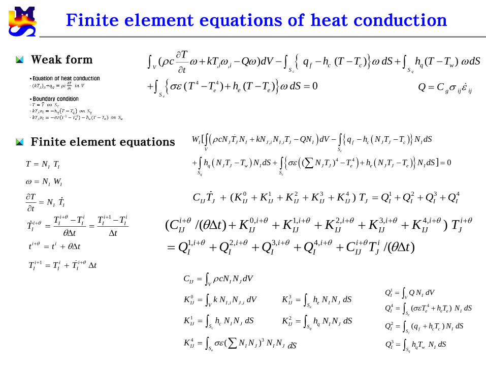
Finite element equations of heat conduction
4 4
, ,( ) ( ) ( )
( ) ( ) 0
c q
e
VS S
eS
i i f c c q w
e e
t
Tc kT Q dV q h T T dS h T T dS
T T h T T dS
Weak form
Finite element equations
g ij ijQ C
I IT N T
I IN W
I I
TN T
t
, ,
4 4( ) 0
[
]
c
q c
I J J I J i I i J I f c J J c I
V S
q J J w I J J e e J J e I
S S
W cN T N kN N T QN dV q h N T T N dS
h N T T N dS N T T h N T T N dS
0 1 2 3 4 1 2 3 4( )IJ J IJ IJ IJ IJ IJ J I I I IC T K K K K K T Q Q Q Q
1
I IV
Q Q N dV
2 ( )c
I f c c IS
Q q h T N dS 3
qI q w I
SQ h T N dS
4 4( )e
I e e e IS
Q T h T N dS
1i i i i
i I I I I
I
T T T TT
t t
0, 1, 2, 3, 4,
1, 2, 3, 4,
( /( ) )
/( )
i i i i i i i
IJ IJ IJ IJ IJ IJ J
i i i i i i
I I I I IJ J
C t K K K K K T
Q Q Q Q C T t
i it t t
1i i i
I I IT T T t
IJ I JV
C cN N dV 0
, ,IJ I i J iV
K k N N dV 1
cIJ c I J
SK h N N dS
2
qIJ q I J
SK h N N dS
3
eIJ e I J
SK h N N dS
4 3( )e
IJ I J I JS
K N N N N dV
- 25 -
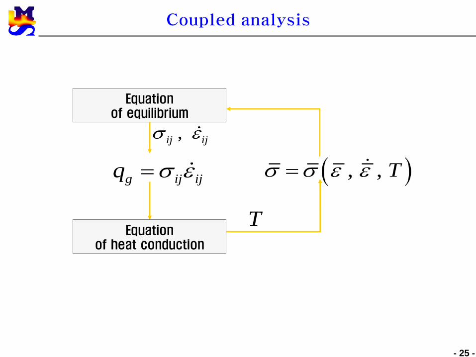
Coupled analysis
T
,ij ij
g ij ijq , , T
Equation of equilibrium
Equation of heat conduction


![A Laguerre-Legendre Spectral-Element Method for the …...spectral methods [3]. As in the finite-element method, a weak statement is constructed and the domain is decomposed into finite](https://img.dokumen.tips/doc/110x75/604cca2f21fdcf39c05413e6/a-laguerre-legendre-spectral-element-method-for-the-spectral-methods-3-as.jpg)