Uttam Reddy - dbmanagement.infodbmanagement.info/Books/MIX/W.H._Inmon_Building_the_Data_Wareh… · Exploration and Data Mining 53 Living Sample Database 53 Partitioning as a Design

TEAMFLY

Team-Fly®

Uttam Reddy

John Wiley & Sons, Inc.NEW YORK • CHICHESTER • WEINHEIM • BRISBANE • SINGAPORE • TORONTO

Wiley Computer Publishing

W. H. Inmon

Building the Data Warehouse

Third Edition

Uttam Reddy

Uttam Reddy


Third Edition

Uttam Reddy

Uttam Reddy

John Wiley & Sons, Inc.NEW YORK • CHICHESTER • WEINHEIM • BRISBANE • SINGAPORE • TORONTO

Wiley Computer Publishing

W. H. Inmon


Third Edition

Uttam Reddy

Publisher: Robert IpsenEditor: Robert ElliottDevelopmental Editor: Emilie HermanManaging Editor: John AtkinsText Design & Composition: MacAllister Publishing Services, LLC

Designations used by companies to distinguish their products are often claimed as trademarks. In allinstances where John Wiley & Sons, Inc., is aware of a claim, the product names appear in initial cap-ital or ALL CAPITAL LETTERS. Readers, however, should contact the appropriate companies for more com-plete information regarding trademarks and registration.

This book is printed on acid-free paper.

Copyright © 2002 by W.H. Inmon. All rights reserved.

Published by John Wiley & Sons, Inc.

Published simultaneously in Canada.

No part of this publication may be reproduced, stored in a retrieval system or transmitted in any formor by any means, electronic, mechanical, photocopying, recording, scanning or otherwise, except aspermitted under Sections 107 or 108 of the 1976 United States Copyright Act, without either the priorwritten permission of the Publisher, or authorization through payment of the appropriate per-copy feeto the Copyright Clearance Center, 222 Rosewood Drive, Danvers, MA 01923, (978) 750-8400, fax (978)750-4744. Requests to the Publisher for permission should be addressed to the Permissions Depart-ment, John Wiley & Sons, Inc., 605 Third Avenue, New York, NY 10158-0012, (212) 850-6011, fax (212)850-6008, E-Mail: PERMREQ @ WILEY.COM.

This publication is designed to provide accurate and authoritative information in regard to the subjectmatter covered. It is sold with the understanding that the publisher is not engaged in professional ser-vices. If professional advice or other expert assistance is required, the services of a competent pro-fessional person should be sought.

Library of Congress Cataloging-in-Publication Data:

ISBN: 0-471-08130-2

Printed in the United States of America.

10 9 8 7 6 5 4 3 2 1

Uttam Reddy

To Jeanne Friedman—a friend for all times

Uttam Reddy

Uttam Reddy

C O N T E N TS

Preface for the Second Edition xiii

Preface for the Third Edition xiv

Acknowledgments xix

About the Author xx

Chapter 1 Evolution of Decision Support Systems 1

The Evolution 2The Advent of DASD 4PC/4GL Technology 4Enter the Extract Program 5The Spider Web 6

Problems with the Naturally Evolving Architecture 6Lack of Data Credibility 6Problems with Productivity 9From Data to Information 12A Change in Approach 15

The Architected Environment 16Data Integration in the Architected Environment 19

Who Is the User? 19

The Development Life Cycle 21

Patterns of Hardware Utilization 22

Setting the Stage for Reengineering 23

Monitoring the Data Warehouse Environment 25

Summary 28

Chapter 2 The Data Warehouse Environment 31

The Structure of the Data Warehouse 35

Subject Orientation 36

Day 1-Day n Phenomenon 41

Granularity 43The Benefits of Granularity 45An Example of Granularity 46Dual Levels of Granularity 49

vii

Uttam Reddy

Exploration and Data Mining 53

Living Sample Database 53

Partitioning as a Design Approach 55Partitioning of Data 56

Structuring Data in the Data Warehouse 59

Data Warehouse: The Standards Manual 64

Auditing and the Data Warehouse 64

Cost Justification 65Justifying Your Data Warehouse 66

Data Homogeneity/Heterogeneity 69

Purging Warehouse Data 72

Reporting and the Architected Environment 73

The Operational Window of Opportunity 74

Incorrect Data in the Data Warehouse 76

Summary 77

Chapter 3 The Data Warehouse and Design 81

Beginning with Operational Data 82

Data/Process Models and the Architected Environment 87

The Data Warehouse and Data Models 89The Data Warehouse Data Model 92The Midlevel Data Model 94The Physical Data Model 98

The Data Model and Iterative Development 102

Normalization/Denormalization 102Snapshots in the Data Warehouse 110

Meta Data 113Managing Reference Tables in a Data Warehouse 113

Cyclicity of Data-The Wrinkle of Time 115

Complexity of Transformation and Integration 118

Triggering the Data Warehouse Record 122Events 122Components of the Snapshot 123Some Examples 123

Profile Records 124

Managing Volume 126

Creating Multiple Profile Records 127

C O N T E N TSviii

TEAMFLY

Team-Fly®

Uttam Reddy

Going from the Data Warehouse to the Operational Environment 128

Direct Access of Data Warehouse Data 129

Indirect Access of Data Warehouse Data 130An Airline Commission Calculation System 130A Retail Personalization System 132Credit Scoring 133

Indirect Use of Data Warehouse Data 136

Star Joins 137

Supporting the ODS 143

Summary 145

Chapter 4 Granularity in the Data Warehouse 147

Raw Estimates 148

Input to the Planning Process 149

Data in Overflow? 149Overflow Storage 151

What the Levels of Granularity Will Be 155

Some Feedback Loop Techniques 156

Levels of Granularity-Banking Environment 158

Summary 165

Chapter 5 The Data Warehouse and Technology 167

Managing Large Amounts of Data 167

Managing Multiple Media 169

Index/Monitor Data 169

Interfaces to Many Technologies 170

Programmer/Designer Control of Data Placement 171

Parallel Storage/Management of Data 171Meta Data Management 171

Language Interface 173

Efficient Loading of Data 173

Efficient Index Utilization 175

Compaction of Data 175

Compound Keys 176

Variable-Length Data 176

Lock Management 176

CONTENTS ix

Uttam Reddy

Index-Only Processing 178

Fast Restore 178

Other Technological Features 178

DBMS Types and the Data Warehouse 179

Changing DBMS Technology 181

Multidimensional DBMS and the Data Warehouse 182

Data Warehousing across Multiple Storage Media 188

Meta Data in the Data Warehouse Environment 189

Context and Content 192Three Types of Contextual Information 193

Capturing and Managing Contextual Information 194Looking at the Past 195

Refreshing the Data Warehouse 195

Testing 198

Summary 198

Chapter 6 The Distributed Data Warehouse 201

Types of Distributed Data Warehouses 202Local and Global Data Warehouses 202The Technologically Distributed Data Warehouse 220The Independently Evolving Distributed Data Warehouse 221

The Nature of the Development Efforts 222Completely Unrelated Warehouses 224

Distributed Data Warehouse Development 226Coordinating Development across Distributed Locations 227The Corporate Data Model-Distributed 228Meta Data in the Distributed Warehouse 232

Building the Warehouse on Multiple Levels 232

Multiple Groups Building the Current Level of Detail 235Different Requirements at Different Levels 238Other Types of Detailed Data 239Meta Data 244

Multiple Platforms for Common Detail Data 244

Summary 245

Chapter 7 Executive Information Systems and the Data Warehouse 247

EIS-The Promise 248

A Simple Example 248

Drill-Down Analysis 251

C O N T E N TSx

Uttam Reddy

Supporting the Drill-Down Process 253

The Data Warehouse as a Basis for EIS 254

Where to Turn 256

Event Mapping 258

Detailed Data and EIS 261Keeping Only Summary Data in the EIS 262

Summary 263

Chapter 8 External/Unstructured Data and the Data Warehouse 265

External/Unstructured Data in the Data Warehouse 268

Meta Data and External Data 269

Storing External/Unstructured Data 271

Different Components of External/Unstructured Data 272

Modeling and External/Unstructured Data 273

Secondary Reports 274

Archiving External Data 275

Comparing Internal Data to External Data 275

Summary 276

Chapter 9 Migration to the Architected Environment 277

A Migration Plan 278

The Feedback Loop 286

Strategic Considerations 287

Methodology and Migration 289

A Data-Driven Development Methodology 291

Data-Driven Methodology 293

System Development Life Cycles 294

A Philosophical Observation 294

Operational Development/DSS Development 294

Summary 295

Chapter 10 The Data Warehouse and the Web 297

Supporting the Ebusiness Environment 307

Moving Data from the Web to the Data Warehouse 307

Moving Data from the Data Warehouse to the Web 308

Web Support 309

Summary 310

CONTENTS xi

Uttam Reddy

Chapter 11 ERP and the Data Warehouse 311

ERP Applications Outside the Data Warehouse 312

Building the Data Warehouse inside the ERP Environment 314

Feeding the Data Warehouse through ERP and Non-ERP Systems 314

The ERP-Oriented Corporate Data Warehouse 318

Summary 320

Chapter 12 Data Warehouse Design Review Checklist 321

When to Do Design Review 322Who Should Be in the Design Review? 323What Should the Agenda Be? 323The Results 323Administering the Review 324A Typical Data Warehouse Design Review 324

Summary 342

Appendix 343

Glossary 385

Reference 397

Index 407

C O N T E N TSXII

Uttam Reddy

Introduction xiii

Databases and database theory have been around for a long time. Early rendi-tions of databases centered around a single database serving every purposeknown to the information processing community—from transaction to batchprocessing to analytical processing. In most cases, the primary focus of theearly database systems was operational—usually transactional—processing. Inrecent years, a more sophisticated notion of the database has emerged—onethat serves operational needs and another that serves informational or analyti-cal needs. To some extent, this more enlightened notion of the database is dueto the advent of PCs, 4GL technology, and the empowerment of the end user.

The split of operational and informational databases occurs for many reasons:

■■ The data serving operational needs is physically different data from thatserving informational or analytic needs.

■■ The supporting technology for operational processing is fundamentally dif-ferent from the technology used to support informational or analyticalneeds.

■■ The user community for operational data is different from the one servedby informational or analytical data.

■■ The processing characteristics for the operational environment and theinformational environment are fundamentally different.

Because of these reasons (and many more), the modern way to build systems isto separate the operational from the informational or analytical processing anddata.

This book is about the analytical [or the decision support systems (DSS)] envi-ronment and the structuring of data in that environment. The focus of the bookis on what is termed the “data warehouse” (or “information warehouse”), whichis at the heart of informational, DSS processing.

The discussions in this book are geared to the manager and the developer.Where appropriate, some level of discussion will be at the technical level. But,for the most part, the book is about issues and techniques. This book is meantto serve as a guideline for the designer and the developer.

PREFACE FOR THE SECOND EDITION

xiii

Uttam Reddy

When the first edition of Building the Data Warehouse was printed, the data-base theorists scoffed at the notion of the data warehouse. One theoreticianstated that data warehousing set back the information technology industry 20years. Another stated that the founder of data warehousing should not beallowed to speak in public. And yet another academic proclaimed that datawarehousing was nothing new and that the world of academia had knownabout data warehousing all along although there were no books, no articles, noclasses, no seminars, no conferences, no presentations, no references, nopapers, and no use of the terms or concepts in existence in academia at thattime.

When the second edition of the book appeared, the world was mad for anythingof the Internet. In order to be successful it had to be “e” something—e-business,e-commerce, e-tailing, and so forth. One venture capitalist was known to say,“Why do we need a data warehouse when we have the Internet?”

But data warehousing has surpassed the database theoreticians who wanted toput all data in a single database. Data warehousing survived the dot.com disas-ter brought on by the short-sighted venture capitalists. In an age when technol-ogy in general is spurned by Wall Street and Main Street, data warehousing hasnever been more alive or stronger. There are conferences, seminars, books,articles, consulting, and the like. But mostly there are companies doing datawarehousing, and making the discovery that, unlike the overhyped New Econ-omy, the data warehouse actually delivers, even though Silicon Valley is still ina state of denial.

The third edition of this book heralds a newer and even stronger day for datawarehousing. Today data warehousing is not a theory but a fact of life. Newtechnology is right around the corner to support some of the more exotic needsof a data warehouse. Corporations are running major pieces of their businesson data warehouses. The cost of information has dropped dramatically becauseof data warehouses. Managers at long last have a viable solution to the uglinessof the legacy systems environment. For the first time, a corporate “memory” ofhistorical information is available. Integration of data across the corporation isa real possibility, in most cases for the first time. Corporations are learning how

PREFACE FOR THE THIRD EDITION

xiv

Uttam Reddy

to go from data to information to competitive advantage. In short, data ware-housing has unlocked a world of possibility.

One confusing aspect of data warehousing is that it is an architecture, not atechnology. This frustrates the technician and the venture capitalist alikebecause these people want to buy something in a nice clean box. But data ware-housing simply does not lend itself to being “boxed up.” The difference betweenan architecture and a technology is like the difference between Santa Fe, NewMexico, and adobe bricks. If you drive the streets of Santa Fe you know you arethere and nowhere else. Each home, each office building, each restaurant has adistinctive look that says “This is Santa Fe.” The look and style that make SantaFe distinctive are the architecture. Now, that architecture is made up of suchthings as adobe bricks and exposed beams. There is a whole art to the makingof adobe bricks and exposed beams. And it is certainly true that you could nothave Santa Fe architecture without having adobe bricks and exposed beams.But adobe bricks and exposed beams by themselves do not make an architec-ture. They are independent technologies. For example, you have adobe bricksthroughout the Southwest and the rest of the world that are not Santa Fearchitecture.

Thus it is with architecture and technology, and with data warehousing anddatabases and other technology. There is the architecture, then there is theunderlying technology, and they are two very different things. Unquestionably,there is a relationship between data warehousing and database technology, butthey are most certainly not the same. Data warehousing requires the support ofmany different kinds of technology.

With the third edition of this book, we now know what works and what doesnot. When the first edition was written, there was some experience with devel-oping and using warehouses, but truthfully, there was not the broad base ofexperience that exists today. For example, today we know with certainty thefollowing:

■■ Data warehouses are built under a different development methodologythan applications. Not keeping this in mind is a recipe for disaster.

■■ Data warehouses are fundamentally different from data marts. The two donot mix—they are like oil and water.

■■ Data warehouses deliver on their promise, unlike many overhyped tech-nologies that simply faded away.

■■ Data warehouses attract huge amounts of data, to the point that entirelynew approaches to the management of large amounts of data are required.

But perhaps the most intriguing thing that has been learned about data ware-housing is that data warehouses form a foundation for many other forms of

Preface for the Third Edition xv

Uttam Reddy

processing. The granular data found in the data warehouse can be reshaped andreused. If there is any immutable and profound truth about data warehouses, itis that data warehouses provide an ideal foundation for many other forms ofinformation processing. There are a whole host of reasons why this foundationis so important:

■■ There is a single version of the truth.

■■ Data can be reconciled if necessary.

■■ Data is immediately available for new, unknown uses.

And, finally, data warehousing has lowered the cost of information in the orga-nization. With data warehousing, data is inexpensive to get to and fast toaccess.

Databases and database theory have been around for a long time. Early rendi-tions of databases centered around a single database serving every purposeknown to the information processing community—from transaction to batchprocessing to analytical processing. In most cases, the primary focus of theearly database systems was operational—usually transactional—processing. Inrecent years, a more sophisticated notion of the database has emerged—onethat serves operational needs and another that serves informational or analyti-cal needs. To some extent, this more enlightened notion of the database is dueto the advent of PCs, 4GL technology, and the empowerment of the end user.

The split of operational and informational databases occurs for many reasons:

■■ The data serving operational needs is physically different data from thatserving informational or analytic needs.

■■ The supporting technology for operational processing is fundamentally dif-ferent from the technology used to support informational or analyticalneeds.

■■ The user community for operational data is different from the one servedby informational or analytical data.

■■ The processing characteristics for the operational environment and theinformational environment are fundamentally different.

For these reasons (and many more), the modern way to build systems is to sep-arate the operational from the informational or analytical processing and data.

This book is about the analytical or the DSS environment and the structuring ofdata in that environment. The focus of the book is on what is termed the datawarehouse (or information warehouse), which is at the heart of informational,DSS processing.

What is analytical, informational processing? It is processing that serves theneeds of management in the decision-making process. Often known as DSS pro-

Preface for the Third Editionxvi

Uttam Reddy

Preface for the Third Edition xvii

cessing, analytical processing looks across broad vistas of data to detecttrends. Instead of looking at one or two records of data (as is the case in oper-ational processing), when the DSS analyst does analytical processing, manyrecords are accessed.

It is rare for the DSS analyst to update data. In operational systems, data is con-stantly being updated at the individual record level. In analytical processing,records are constantly being accessed, and their contents are gathered foranalysis, but little or no alteration of individual records occurs.

In analytical processing, the response time requirements are greatly relaxedcompared to those of traditional operational processing. Analytical responsetime is measured from 30 minutes to 24 hours. Response times measured in thisrange for operational processing would be an unmitigated disaster.

The network that serves the analytical community is much smaller than the onethat serves the operational community. Usually there are far fewer users of theanalytical network than of the operational network.

Unlike the technology that serves the analytical environment, operational envi-ronment technology must concern itself with data and transaction locking, con-tention for data, deadlock, and so on.

There are, then, many major differences between the operational environmentand the analytical environment. This book is about the analytical, DSS environ-ment and addresses the following issues:

■■ Granularity of data

■■ Partitioning of data

■■ Meta data

■■ Lack of credibility of data

■■ Integration of DSS data

■■ The time basis of DSS data

■■ Identifying the source of DSS data-the system of record

■■ Migration and methodology

This book is for developers, managers, designers, data administrators, databaseadministrators, and others who are building systems in a modern data process-ing environment. In addition, students of information processing will find thisbook useful. Where appropriate, some discussions will be more technical. But,for the most part, the book is about issues and techniques, and it is meant toserve as a guideline for the designer and the developer.

Uttam Reddy

This book is the first in a series of books relating to data warehouse. The nextbook in the series is Using the Data Warehouse (Wiley, 1994). Using the Data

Warehouse addresses the issues that arise once you have built the data ware-house. In addition, Using the Data Warehouse introduces the concept of alarger architecture and the notion of an operational data store (ODS). An oper-ational data store is a similar architectural construct to the data warehouse,except the ODS applies only to operational systems, not informational systems.The third book in the series is Building the Operational Data Store (Wiley,1999), which addresses the issues of what an ODS is and how an ODS is built.

The next book in the series is Corporate Information Factory, Third Edition

(Wiley, 2002). This book addresses the larger framework of which the datawarehouse is the center. In many regards the CIF book and the DW book arecompanions. The CIF book provides the larger picture and the DW bookprovides a more focused discussion. Another related book is Exploration

Warehousing (Wiley, 2000). This book addresses a specialized kind of process-ing-pattern analysis using statistical techniques on data found in the datawarehouse.

Building the Data Warehouse, however, is the cornerstone of all the relatedbooks. The data warehouse forms the foundation of all other forms of DSSprocessing.

There is perhaps no more eloquent testimony to the advances made by datawarehousing and the corporate information factory than the References at theback of this book. When the first edition was published, there were no otherbooks, no white papers, and only a handful of articles that could be referenced.In this third edition, there are many books, articles, and white papers that arementioned. Indeed the references only start to explore some of the more impor-tant works.

Preface for the Third Editionxviii

TEAMFLY

Team-Fly®

Uttam Reddy

Introduction xix

The following people have influenced—directly and indirectly—the materialfound in this book. The author is grateful for the long-term relationships thathave been formed and for the experiences that have provided a basis forlearning.

Claudia Imhoff, Intelligent Solutions

Jon Geiger, Intelligent Solutions

Joyce Norris Montanari, Intelligent Solutions

John Zachman, Zachman International

John Ladley, Meta Group

Bob Terdeman, EMC Corporation

Dan Meers, BillInmon.com

Cheryl Estep, independent consultant

Lowell Fryman, independent consultant

David Fender, SAS Japan

Jim Davis, SAS

Peter Grendel, SAP

Allen Houpt, CA

A C K N O W L E D G M E N TS

xix

Uttam Reddy

Bill Inmon, the father of the data warehouse concept, has written 40 books ondata management, data warehouse, design review, and management of dataprocessing. Bill has had his books translated into Russian, German, French,Japanese, Portuguese, Chinese, Korean, and Dutch. Bill has published morethan 250 articles in many trade journals. Bill founded and took public PrismSolutions. His latest company—Pine Cone Systems—builds software for themanagement of the data warehouse/data mart environment. Bill holds two soft-ware patents. Articles, white papers, presentations, and much more materialcan be found on his Web site, www.billinmon.com.

A B O U T T H E A U T H O R

xx

Uttam Reddy

Evolution of Decision Support Systems

C H A P T E R 1

We are told that the hieroglyphics in Egypt are primarily the work of an accoun-tant declaring how much grain is owed the Pharaoh. Some of the streets inRome were laid out by civil engineers more than 2,000 years ago. Examina-tion of bones found in archeological excavations shows that medicine—in, atleast, a rudimentary form—was practiced as long as 10,000 years ago. Otherprofessions have roots that can be traced back to antiquity. From this per-spective, the profession and practice of information systems and processingis certainly immature, because it has existed only since the early 1960s.

Information processing shows this immaturity in many ways, such as its ten-dency to dwell on detail. There is the notion that if we get the details right, theend result will somehow take care of itself and we will achieve success. It’slike saying that if we know how to lay concrete, how to drill, and how toinstall nuts and bolts, we don’t have to worry about the shape or the use of thebridge we are building. Such an attitude would drive a more professionallymature civil engineer crazy. Getting all the details right does not necessarilybring more success.

The data warehouse requires an architecture that begins by looking at thewhole and then works down to the particulars. Certainly, details are impor-tant throughout the data warehouse. But details are important only whenviewed in a broader context.

1

Uttam Reddy

The story of the data warehouse begins with the evolution of information anddecision support systems. This broad view should help put data warehousinginto clearer perspective.

The Evolution

The origins of DSS processing hark back to the very early days of computersand information systems. It is interesting that decision support system (DSS)processing developed out of a long and complex evolution of information tech-nology. Its evolution continues today.

Figure 1.1 shows the evolution of information processing from the early 1960sup to 1980. In the early 1960s, the world of computation consisted of creatingindividual applications that were run using master files. The applications fea-tured reports and programs, usually built in COBOL. Punched cards were com-mon. The master files were housed on magnetic tape, which were good forstoring a large volume of data cheaply, but the drawback was that they had tobe accessed sequentially. In a given pass of a magnetic tape file, where 100 per-cent of the records have to be accessed, typically only 5 percent or fewer of therecords are actually needed. In addition, accessing an entire tape file may takeas long as 20 to 30 minutes, depending on the data on the file and the process-ing that is done.

Around the mid-1960s, the growth of master files and magnetic tape exploded.And with that growth came huge amounts of redundant data. The proliferationof master files and redundant data presented some very insidious problems:

■■ The need to synchronize data upon update

■■ The complexity of maintaining programs

■■ The complexity of developing new programs

■■ The need for extensive amounts of hardware to support all the master files

In short order, the problems of master files—problems inherent to the mediumitself—became stifling.

It is interesting to speculate what the world of information processing wouldlook like if the only medium for storing data had been the magnetic tape. Ifthere had never been anything to store bulk data on other than magnetic tape

C H A P T E R 12

Uttam Reddy

Evolution of Decision Support Systems 3

1975online, high-performancetransaction processing

the single-database-serving-all-purposes paradigm

PCs, 4GL technology

MIS/DSStx processing

1970database— “a single source of

data for all processing”

1965

lots of master files !!!

• complexity of—• maintenance• development

• synchronization of data• hardware

master files, reports1960

1980

DASD

DBMS

Figure 1.1 The early evolutionary stages of the architected environment.

Uttam Reddy

files, the world would have never had large, fast reservations systems, ATM sys-tems, and the like. Indeed, the ability to store and manage data on new kinds ofmedia opened up the way for a more powerful type of processing that broughtthe technician and the businessperson together as never before.

The Advent of DASDBy 1970, the day of a new technology for the storage and access of data haddawned. The 1970s saw the advent of disk storage, or direct access storagedevice (DASD). Disk storage was fundamentally different from magnetic tapestorage in that data could be accessed directly on DASD. There was no need togo through records 1, 2, 3, . . . n to get to record n � 1. Once the address ofrecord n � 1 was known, it was a simple matter to go to record n � 1 directly.Furthermore, the time required to go to record n � 1 was significantly less thanthe time required to scan a tape. In fact, the time to locate a record on DASDcould be measured in milliseconds.

With DASD came a new type of system software known as a database manage-ment system (DBMS). The purpose of the DBMS was to make it easy for theprogrammer to store and access data on DASD. In addition, the DBMS tookcare of such tasks as storing data on DASD, indexing data, and so forth. WithDASD and DBMS came a technological solution to the problems of master files.And with the DBMS came the notion of a “database.” In looking at the mess thatwas created by master files and the masses of redundant data aggregated onthem, it is no wonder that in the 1970s a database was defined as a single sourceof data for all processing.

By the mid-1970s, online transaction processing (OLTP) made even fasteraccess to data possible, opening whole new vistas for business and processing.The computer could now be used for tasks not previously possible, includingdriving reservations systems, bank teller systems, manufacturing control sys-tems, and the like. Had the world remained in a magnetic-tape-file state, mostof the systems that we take for granted today would not have been possible.

PC/4GL TechnologyBy the 1980s, more new technologies, such as PCs and fourth-generation lan-guages (4GLs), began to surface. The end user began to assume a role previ-ously unfathomed—directly controlling data and systems—a role previouslyreserved for the data processor. With PCs and 4GL technology came the notionthat more could be done with data than simply processing online transactions.MIS (management information systems), as it was called in the early days,could also be implemented. Today known as DSS, MIS was processing used todrive management decisions. Previously, data and technology were used exclu-

C H A P T E R 14

Uttam Reddy

sively to drive detailed operational decisions. No single database could serveboth operational transaction processing and analytical processing at the sametime. Figure 1.1 shows the single-database paradigm.

Enter the Extract ProgramShortly after the advent of massive OLTP systems, an innocuous program for“extract” processing began to appear (see Figure 1.2).

The extract program is the simplest of all programs. It rummages through a fileor database, uses some criteria for selecting data, and, on finding qualified data,transports the data to another file or database.


1985

extract program

Why extract processing?• performance• control

Start with some parameters, search a filebased on the satisfaction of theparameters, then pull the data elsewhere.

extract processing

Figure 1.2 The nature of extract processing.

Uttam Reddy

The extract program became very popular, for at least two reasons:

■■ Because extract processing can move data out of the way of high-performance online processing, there is no conflict in terms of perfor-mance when the data needs to be analyzed en masse.

■■ When data is moved out of the operational, transaction-processing domainwith an extract program, a shift in control of the data occurs. The end userthen owns the data once he or she takes control of it. For these (and prob-ably a host of other) reasons, extract processing was soon found every-where.

The Spider WebAs illustrated in Figure 1.3, a “spider web” of extract processing began to form.First, there were extracts; then there were extracts of extracts; then extracts ofextracts of extracts; and so forth. It was not unusual for a large company to per-form as many as 45,000 extracts per day.

This pattern of out-of-control extract processing across the organizationbecame so commonplace that it was given its own name—the “naturally evolv-ing architecture”—which occurs when an organization handles the wholeprocess of hardware and software architecture with a laissez-faire attitude. Thelarger and more mature the organization, the worse the problems of the natu-rally evolving architecture become.

Problems with the Naturally Evolving Architecture

The naturally evolving architecture presents many challenges, such as:

■■ Data credibility

■■ Productivity

■■ Inability to transform data into information

Lack of Data CredibilityThe lack of data credibility is illustrated in Figure 1.3. Say two departments aredelivering a report to management—one department claims that activity isdown 15 percent, the other says that activity is up 10 percent. Not only are thetwo departments not in sync with each other, they are off by very large margins.In addition, trying to reconcile the departments is difficult. Unless very carefuldocumentation has been done, reconciliation is, for all practical purposes,impossible.

C H A P T E R 16

Uttam Reddy

When management receives the conflicting reports, it is forced to make deci-sions based on politics and personalities because neither source is more or lesscredible. This is an example of the crisis of data credibility in the naturallyevolving architecture.

This crisis is widespread and predictable. Why? As depicted in Figure 1.3, thereare five reasons:

■■ No time basis of data

■■ The algorithmic differential of data

■■ The levels of extraction

■■ The problem of external data

■■ No common source of data from the beginning


Dept. A+10%

Dept. B–15%

• no time basis of data• algorithmic differential• levels of extraction• external data• no common source of data to begin with

Figure 1.3 Lack of data credibility in the naturally evolving architecture.

Uttam Reddy

The first reason for the predictability of the crisis is that there is no time basisfor the data. Figure 1.4 shows such a time discrepancy. One department hasextracted its data for analysis on a Sunday evening, and the other departmentextracted on a Wednesday afternoon. Is there any reason to believe that analy-sis done on one sample of data taken on one day will be the same as the analy-sis for a sample of data taken on another day? Of course not! Data is alwayschanging within the corporation. Any correlation between analyzed sets of datathat are taken at different points in time is only coincidental.

The second reason is the algorithmic differential. For example, one departmenthas chosen to analyze all old accounts. Another department has chosen to ana-

C H A P T E R 18

• Sunday evening• old accts

Dept. B–15%• Wednesday p.m.• large accts

multiplelevels ofextraction

multiplelevels ofextraction

no common sourceof data to begin with

• loss of identity• no coordination with other

people entering external data

Dept. A+10%

WallStreet

Journal

BusinessWeek

Figure 1.4 The reasons for the predictability of the crisis in data credibility in the natu-rally evolving architecture.

TEAMFLY

Team-Fly®

Uttam Reddy

lyze all large accounts. Is there any necessary correlation between the charac-teristics of customers who have old accounts and customers who have largeaccounts? Probably not. So why should a very different result surprise anyone?

The third reason is one that merely magnifies the first two reasons. Every timea new extraction is done, the probabilities of a discrepancy arise because of thetiming or the algorithmic differential. And it is not unusual for a corporation tohave eight or nine levels of extraction being done from the time the data entersthe corporation’s system to the time analysis is prepared for management.There are extracts, extracts of extracts, extracts of extracts of extracts, and soon. Each new level of extraction exaggerates the other problems that occur.

The fourth reason for the lack of credibility is the problem posed by externaldata. With today’s technologies at the PC level, it is very easy to bring in datafrom outside sources. For example, Figure 1.5 shows one analyst bringing datainto the mainstream of analysis from the Wall Street Journal, and another ana-lyst bringing data in from Business Week. However, when the analyst bringsdata in, he or she strips the identity of the external data. Because the origin ofthe data is not captured, it becomes generic data that could have come from anysource.

Furthermore, the analyst who brings in data from the Wall Street Journal

knows nothing about the data being entered from Business Week, and viceversa. No wonder, then, that external data contributes to the lack of credibilityof data in the naturally evolving architecture.

The last contributing factor to the lack of credibility is that often there is nocommon source of data to begin with. Analysis for department A originatesfrom file XYZ. Analysis for department B originates from database ABC. Thereis no synchronization or sharing of data whatsoever between file XYZ and data-base ABC.

Given these reasons, it is no small wonder that there is a crisis of credibilitybrewing in every organization that allows its legacy of hardware, software, anddata to evolve naturally into the spider web.

Problems with ProductivityData credibility is not the only major problem with the naturally evolving archi-tecture. Productivity is also abysmal, especially when there is a need to analyzedata across the organization.

Consider an organization that has been in business for a while and has built upa large collection of data, as shown in the top of Figure 1.5.


Uttam Reddy

Management wants to produce a corporate report, using the many files and col-lections of data that have accumulated over the years. The designer assigned thetask decides that three things must be done to produce the corporate report:

C H A P T E R 110

productivity

Produce a corporate report, across all data.

Lots of extract programs, each customized, have to cross many technological barriers.

Locating the data requires looking at lots of files.

X

X

X

X

X

X

X

X

X

X

X

X

X

X

X

X

X

X

X

X

X

X

X

X

X

X

X

Figure 1.5 The naturally evolving architecture is not conducive to productivity.

Uttam Reddy

■■ Locate and analyze the data for the report.

■■ Compile the data for the report.

■■ Get programmer/analyst resources to accomplish these two tasks.

In order to locate the data, many files and layouts of data must be analyzed.Some files use Virtual Storage Access Method (VSAM), some use InformationManagement System (IMS), some use Adabas, some use Integrated DatabaseManagement System (IDMS). Different skill sets are required in order to accessdata across the enterprise. Furthermore, there are complicating factors: forexample, two files might have an element called BALANCE, but the two ele-ments are very different. In another case, one database might have a file knownas CURRBAL, and another collection of data might have a file called INVLEVELthat happens to represent the same information as CURRBAL. Having to gothrough every piece of data—not just by name but by definition and calcula-tion—is a very tedious process. But if the corporate report is to be produced,this exercise must be done properly. Unless data is analyzed and “rationalized,”the report will end up mixing apples and oranges, creating yet another level ofconfusion.

The next task for producing the report is to compile the data once it is located.The program that must be written to get data from its many sources should besimple. It is complicated, though, by the following facts:

■■ Lots of programs have to be written.

■■ Each program must be customized.

■■ The programs cross every technology that the company uses.

In short, even though the report-generation program should be simple to write,retrieving the data for the report is tedious.

In a corporation facing exactly the problems described, an analyst recently esti-mated a very long time to accomplish the tasks, as shown in Figure 1.6.

If the designer had asked for only two or three man-months of resources, thengenerating the report might not have required much management attention. Butwhen an analyst requisitions many resources, management must consider therequest with all the other requests for resources and must prioritize therequests.

Creating the reports using a large amount of resources wouldn’t be bad if therewere a one-time penalty to be paid. In other words, if the first corporate reportgenerated required a large amount of resources, and if all succeeding reportscould build on the first report, then it might be worthwhile to pay the price forgenerating the first report. But that is not the case.


Uttam Reddy

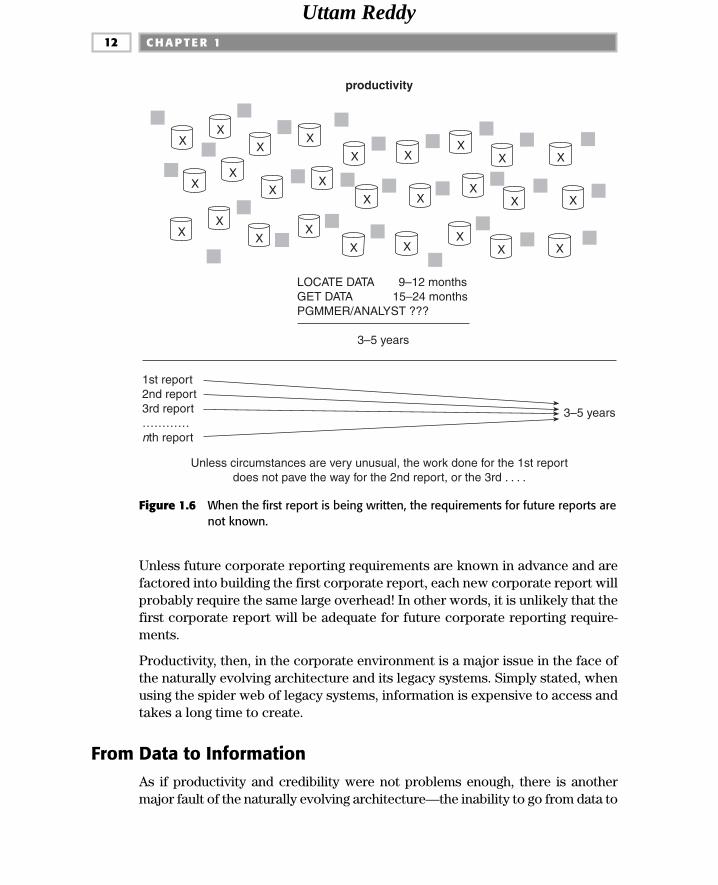
Unless future corporate reporting requirements are known in advance and arefactored into building the first corporate report, each new corporate report willprobably require the same large overhead! In other words, it is unlikely that thefirst corporate report will be adequate for future corporate reporting require-ments.

Productivity, then, in the corporate environment is a major issue in the face ofthe naturally evolving architecture and its legacy systems. Simply stated, whenusing the spider web of legacy systems, information is expensive to access andtakes a long time to create.

From Data to InformationAs if productivity and credibility were not problems enough, there is anothermajor fault of the naturally evolving architecture—the inability to go from data to

C H A P T E R 112

productivity

LOCATE DATA 9–12 monthsGET DATA 15–24 monthsPGMMER/ANALYST ???

3–5 years

1st report2nd report3rd report…………nth report

3–5 years

Unless circumstances are very unusual, the work done for the 1st reportdoes not pave the way for the 2nd report, or the 3rd . . . .

X

X

X

X

X

X

X

X

X

X

X

X

X

X

X

X

X

X

X

X

X

X

X

X

X

X

X

Figure 1.6 When the first report is being written, the requirements for future reports arenot known.

Uttam Reddy

information. At first glance, the notion of going from data to information seemsto be an ethereal concept with little substance. But that is not the case at all.

Consider the following request for information, typical in a banking environ-ment: “How has account activity differed this year from each of the past fiveyears?”

Figure 1.7 shows the request for information.


element existsonly here

same element,different name

different element,same name

going from data to information

First, you run into lots of applications.

loans

DDA

CD

passbook

loans

DDA

CD

passbook

Next, you run into the lack of integration across applications.

Figure 1.7 “How has account activity been different this year from each of the past fiveyears for the financial institution?”

Uttam Reddy

The first thing the DSS analyst discovers in trying to satisfy the request forinformation is that going to existing systems for the necessary data is the worstthing to do. The DSS analyst will have to deal with lots of unintegrated legacyapplications. For example, a bank may have separate savings, loan, direct-deposit, and trust applications. However, trying to draw information from themon a regular basis is nearly impossible because the applications were neverconstructed with integration in mind, and they are no easier for the DSS analystto decipher than they are for anyone else.

But integration is not the only difficulty the analyst meets in trying to satisfy aninformational request. A second major obstacle is that there is not enough his-torical data stored in the applications to meet the needs of the DSS request.

Figure 1.8 shows that the loan department has up to two years’ worth of data.Passbook processing has up to one year of data. DDA applications have up to60 days of data. And CD processing has up to 18 months of data. The applica-tions were built to service the needs of current balance processing. They werenever designed to hold the historical data needed for DSS analysis. It is no won-der, then, that going to existing systems for DSS analysis is a poor choice. Butwhere else is there to go?

The systems found in the naturally evolving architecture are simply inadequatefor supporting information needs. They lack integration and there is a discrep-

C H A P T E R 114

“How has account activity been different this year from each of the past fivefor the financial institution?

loans

currentvalue—2 years

Example of going from data to information:

DDA

currentvalue—30 days

CD

curentvalue—18 monthspassbook

currentvalue—1 year

Figure 1.8 Existing applications simply do not have the historical data required to con-vert data into information.

Uttam Reddy

ancy between the time horizon (or parameter of time) needed for analyticalprocessing and the available time horizon that exists in the applications.

A Change in ApproachThe status quo of the naturally evolving architecture, where most shops began,simply is not robust enough to meet the future needs. What is needed is some-thing much larger—a change in architectures. That is where the architecteddata warehouse comes in.

There are fundamentally two kinds of data at the heart of an “architected” envi-ronment—primitive data and derived data. Figure 1.9 shows some of the majordifferences between primitive and derived data.

Following are some other differences between the two.

■■ Primitive data is detailed data used to run the day-to-day operations of thecompany. Derived data has been summarized or otherwise calculated tomeet the needs of the management of the company.


DERIVED DATA/DSS DATA

• subject oriented• summarized, otherwise refined• represents values over time, snapshots• serves the managerial community• is not updated• run heuristically• requirements for processing not

understood a priori• completely different life cycle• performance relaxed• accessed a set at a time• analysis driven• control of update no issue

• relaxed availability• managed by subsets• redundancy is a fact of life• flexible structure• large amount of data used in a process• supports managerial needs• low, modest probability of access

PRIMITIVE DATA/OPERATIONAL DATA

• application oriented• detailed• accurate, as of the moment of access• serves the clerical community• can be updated• run repetitively• requirements for processing understood

a priori• compatible with the SDLC• performance sensitive• accessed a unit at a time• transaction driven• control of update a major concern in

terms of ownership• high availability• managed in its entirety• nonredundancy• static structure; variable contents• small amount of data used in a process• supports day-to-day operations• high probability of access

Figure 1.9 The whole notion of data is changed in the architected environment.

Uttam Reddy

■■ Primitive data can be updated. Derived data can be recalculated but cannotbe directly updated.

■■ Primitive data is primarily current-value data. Derived data is often histori-cal data.

■■ Primitive data is operated on by repetitive procedures. Derived data isoperated on by heuristic, nonrepetitive programs and procedures.

■■ Operational data is primitive; DSS data is derived.

■■ Primitive data supports the clerical function. Derived data supports themanagerial function.

It is a wonder that the information processing community ever thought thatboth primitive and derived data would fit and peacefully coexist in a singledatabase. In fact, primitive data and derived data are so different that they donot reside in the same database or even the same environment.

The Architected Environment

The natural extension of the split in data caused by the difference betweenprimitive and derived data is shown in Figure 1.10.

C H A P T E R 116

levels of the architecture

• detailed• day to day• current valued• high probability

of access• application oriented

• most granular• time variant• integrated• subject oriented• some summary

• parochial• some derived;

some primitive• typical depts

• acctg• marketing• engineering• actuarial• manufacturing

• temporary• ad hoc• heuristic• non-

repetitive• PC, work-

stationbased

operational atomic/datawarehouse

departmental individual

Figure 1.10 Although it is not apparent at first glance, there is very little redundancy ofdata across the architected environment.

Uttam Reddy

There are four levels of data in the architected environment—the operationallevel, the atomic or the data warehouse level, the departmental (or the datamart level), and the individual level. These different levels of data are the basisof a larger architecture called the corporate information factory. The opera-tional level of data holds application-oriented primitive data only and primarilyserves the high-performance transaction-processing community. The data-warehouse level of data holds integrated, historical primitive data that cannotbe updated. In addition, some derived data is found there. The departmental/data mart level of data contains derived data almost exclusively. The depart-mental/data mart level of data is shaped by end-user requirements into a formspecifically suited to the needs of the department. And the individual level ofdata is where much heuristic analysis is done.

The different levels of data form a higher set of architectural entities. Theseentities constitute the corporate information factory, and they are described inmore detail in my book The Corporate Information Factory, Third Edition

(Wiley, 2002).

Some people believe the architected environment generates too much redun-dant data. Though it is not obvious at first glance, this is not the case at all.Instead, it is the spider web environment that generates the gross amounts ofdata redundancy.

Consider the simple example of data throughout the architecture, shown in Fig-ure 1.11. At the operational level there is a record for a customer, J Jones. Theoperational-level record contains current-value data that can be updated at amoment’s notice and shows the customer’s current status. Of course, if theinformation for J Jones changes, the operational-level record will be changed toreflect the correct data.

The data warehouse environment contains several records for J Jones, whichshow the history of information about J Jones. For example, the data ware-house would be searched to discover where J Jones lived last year. There is nooverlap between the records in the operational environment, where currentinformation is found, and the data warehouse environment, where historicalinformation is found. If there is a change of address for J Jones, then a newrecord will be created in the data warehouse, reflecting the from and to datesthat J Jones lived at the previous address. Note that the records in the datawarehouse do not overlap. Also note that there is some element of time associ-ated with each record in the data warehouse.

The departmental environment—sometimes called the data mart level, theOLAP level, or the multidimensional DBMS level—contains information usefulto the different parochial departments of a company. There is a marketing departmental database, an accounting departmental database, an actuarial


Uttam Reddy

departmental database, and so forth. The data warehouse is the source of alldepartmental data. While data in the data mart certainly relates to data found inthe operational level or the data warehouse, the data found in the departmen-tal/data mart environment is fundamentally different from the data found in thedata mart environment, because data mart data is denormalized, summarized,and shaped by the operating requirements of a single department.

Typical of data at the departmental/data mart level is a monthly customer file.In the file is a list of all customers by category. J Jones is tallied into this sum-mary each month, along with many other customers. It is a stretch to considerthe tallying of information to be redundant.

The final level of data is the individual level. Individual data is usually tempo-rary and small. Much heuristic analysis is done at the individual level. As a rule,

C H A P T E R 118

J Jones1987–1989456 High StCredit - A

J Jones123 MainStreetCredit - AA

J Jones1986–1987456 High StCredit - B

J Jones1989–pres123 Main StCredit - AA

Jan - 4101Feb - 4209Mar - 4175Apr - 4215..................................

customerssince 1982with acctbalances> 5,000 andwith creditratings of Bor higher

J Jones1987–1989456 High StCredit - A

J Jones123 MainStreetCredit - AA

J Jones1986–1987456 High StCredit - B

temporary!

What is J Jonescredit rating rightnow?

What has been thecredit history of JJones?

Are we attractingmore or fewercustomers overtime?

What trends arethere for thecustomers we areanalyzing?

a simple example—a customer


dept/data martcustomers by month

individual

J Jones1989–pres123 Main StCredit - AA

Jan - 4101Feb - 4209Mar - 4175Apr - 4215..................................

customerssince 1982with acctbalances> 5,000 andwith creditratings of Bor higher

Figure 1.11 The kinds of queries for which the different levels of data can be used.TEAMFLY

Team-Fly®

Uttam Reddy

the individual levels of data are supported by the PC. Executive informationsystems (EIS) processing typically runs on the individual levels.

Data Integration in the Architected Environment

One important aspect of the architected environment that is not shown in Fig-ure 1.11 is the integration of data that occurs across the architecture. As datapasses from the operational environment to the data warehouse environment,it is integrated, as shown in Figure 1.12.

There is no point in bringing data over from the operational environment intothe data warehouse environment without integrating it. If the data arrives at thedata warehouse in an unintegrated state, it cannot be used to support a corpo-rate view of data. And a corporate view of data is one of the essences of thearchitected environment.

In every environment the unintegrated operational data is complex and difficultto deal with. This is simply a fact of life. And the task of getting one’s hands dirtywith the process of integration is never pleasant. In order to achieve the realbenefits of a data warehouse, though, it is necessary to undergo this painful,complex, and time-consuming exercise. Extract/transform/load (ETL) softwarecan automate much of this tedious process. In addition, this process of integra-tion has to be done only once. But, in any case, it is mandatory that data flow-ing into the data warehouse be integrated, not merely tossed—wholecloth—into the data warehouse from the operational environment.

Who Is the User?

Much about the data warehouse is fundamentally different from the operationalenvironment. When developers and designers who have spent their entirecareers in the operational environment first encounter the data warehouse,they often feel ill at ease. To help them appreciate why there is such a differencefrom the world they have known, they should understand a little bit about thedifferent users of the data warehouse.

The data-warehouse user—also called the DSS analyst—is a businesspersonfirst and foremost, and a technician second. The primary job of the DSS analystis to define and discover information used in corporate decision-making.

It is important to peer inside the head of the DSS analyst and view how he orshe perceives the use of the data warehouse. The DSS analyst has a mindset of“Give me what I say I want, then I can tell you what I really want.” In otherwords, the DSS analyst operates in a mode of discovery. Only on seeing a report


Uttam Reddy

or seeing a screen can the DSS analyst begin to explore the possibilities forDSS. The DSS analyst often says, “Ah! Now that I see what the possibilities are,I can tell you what I really want to see. But until I know what the possibilitiesare I cannot describe to you what I want.”

C H A P T E R 120

life policy

J JonesfemaleJuly 20, 1945...................

customer

J JonesfemaleJuly 20, 1945—dobtwo tickets last yearone bad accident123 Main Streetmarriedtwo childrenhigh blood pressure....................

a simple example—a customer


auto policy

J Jonestwo tickets last yearone bad accident....................

homeowner policy

J Jones123 Main Streetmarried...................

health policy

J Jonestwo childrenhigh blood pressure....................

Figure 1.12 As data is transformed from the operational environment to the data ware-house environment, it is also integrated.

Uttam Reddy

The attitude of the DSS analyst is important for the following reasons:

■■ It is legitimate. This is simply how DSS analysts think and how they con-duct their business.

■■ It is pervasive. DSS analysts around the world think like this.

■■ It has a profound effect on the way the data warehouse is developed andon how systems using the data warehouse are developed.

The classical system development life cycle (SDLC) does not work in the worldof the DSS analyst. The SDLC assumes that requirements are known at the startof design (or at least can be discovered). In the world of the DSS analyst,though, new requirements usually are the last thing to be discovered in the DSSdevelopment life cycle. The DSS analyst starts with existing requirements, butfactoring in new requirements is almost an impossibility. A very different devel-opment life cycle is associated with the data warehouse.

The Development Life Cycle

We have seen how operational data is usually application oriented and as a con-sequence is unintegrated, whereas data warehouse data must be integrated.Other major differences also exist between the operational level of data andprocessing and the data warehouse level of data and processing. The underly-ing development life cycles of these systems can be a profound concern, asshown in Figure 1.13.

Figure 1.13 shows that the operational environment is supported by the classi-cal systems development life cycle (the SDLC). The SDLC is often called the“waterfall” development approach because the different activities are specifiedand one activity-upon its completion-spills down into the next activity and trig-gers its start.

The development of the data warehouse operates under a very different lifecycle, sometimes called the CLDS (the reverse of the SDLC). The classicalSDLC is driven by requirements. In order to build systems, you must first under-stand the requirements. Then you go into stages of design and development.The CLDS is almost exactly the reverse: The CLDS starts with data. Once thedata is in hand, it is integrated and then tested to see what bias there is to thedata, if any. Programs are then written against the data. The results of the pro-grams are analyzed, and finally the requirements of the system are understood.The CLDS is usually called a “spiral” development methodology. A spiral devel-opment methodology is included on the Web site, www.billinmon.com.


Uttam Reddy

The CLDS is a classic data-driven development life cycle, while the SDLC is aclassic requirements-driven development life cycle. Trying to apply inappropri-ate tools and techniques of development results only in waste and confusion.For example, the CASE world is dominated by requirements-driven analysis.Trying to apply CASE tools and techniques to the world of the data warehouseis not advisable, and vice versa.

Patterns of Hardware Utilization

Yet another major difference between the operational and the data warehouseenvironments is the pattern of hardware utilization that occurs in each envi-ronment. Figure 1.14 illustrates this.

The left side of Figure 1.14 shows the classic pattern of hardware utilization foroperational processing. There are peaks and valleys in operational processing,but ultimately there is a relatively static and predictable pattern of hardwareutilization.

C H A P T E R 122

classical SDLC

• requirements gathering• analysis• design• programming• testing• integration• implementation

data warehouse SDLC

• implement warehouse• integrate data• test for bias• program against data• design DSS system• analyze results• understand requirements

program

program

datawarehouse

requirements

requirements

Figure 1.13 The system development life cycle for the data warehouse environment isalmost exactly the opposite of the classical SDLC.

Uttam Reddy

There is an essentially different pattern of hardware utilization in the datawarehouse environment (shown on the right side of the figure)—a binary pat-tern of utilization. Either the hardware is being utilized fully or not at all. It isnot useful to calculate a mean percentage of utilization for the data warehouseenvironment. Even calculating the moments when the data warehouse is heav-ily used is not particularly useful or enlightening.

This fundamental difference is one more reason why trying to mix the two envi-ronments on the same machine at the same time does not work. You can optimizeyour machine either for operational processing or for data warehouse process-ing, but you cannot do both at the same time on the same piece of equipment.

Setting the Stage for Reengineering

Although indirect, there is a very beneficial side effect of going from the pro-duction environment to the architected, data warehouse environment. Fig-ure 1.15 shows the progression.

In Figure 1.15, a transformation is made in the production environment. Thefirst effect is the removal of the bulk of data—mostly archival—from the pro-duction environment. The removal of massive volumes of data has a beneficialeffect in various ways. The production environment is easer to:

■■ Correct

■■ Restructure

■■ Monitor

■■ Index

In short, the mere removal of a significant volume of data makes the productionenvironment a much more malleable one.

Another important effect of the separation of the operational and the datawarehouse environments is the removal of informational processing from the


100%

0%

operational data warehouse

Figure 1.14 The different patterns of hardware utilization in the different environments.

Uttam Reddy

production environment. Informational processing occurs in the form ofreports, screens, extracts, and so forth. The very nature of information pro-cessing is constant change. Business conditions change, the organizationchanges, management changes, accounting practices change, and so on. Eachof these changes has an effect on summary and informational processing. Wheninformational processing is included in the production, legacy environment,maintenance seems to be eternal. But much of what is called maintenance inthe production environment is actually informational processing goingthrough the normal cycle of changes. By moving most informational process-ing off to the data warehouse, the maintenance burden in the production envi-ronment is greatly alleviated. Figure 1.16 shows the effect of removing volumesof data and informational processing from the production environment.

Once the production environment undergoes the changes associated withtransformation to the data warehouse-centered, architected environment, theproduction environment is primed for reengineering because:

■■ It is smaller.

■■ It is simpler.

■■ It is focused.

In summary, the single most important step a company can take to makeits efforts in reengineering successful is to first go to the data warehouseenvironment.

C H A P T E R 124

operationalenvironment

data warehouseenvironment

productionenvironment

Figure 1.15 The transformation from the legacy systems environment to the archi-tected, data warehouse-centered environment.

Uttam Reddy

Monitoring the Data Warehouse Environment

Once the data warehouse is built, it must be maintained. A major component ofmaintaining the data warehouse is managing performance, which begins bymonitoring the data warehouse environment.

Two operating components are monitored on a regular basis: the data residingin the data warehouse and the usage of the data. Monitoring the data in the datawarehouse environment is essential to effectively manage the data warehouse.Some of the important results that are achieved by monitoring this data includethe following:

■■ Identifying what growth is occurring, where the growth is occurring, and atwhat rate the growth is occurring

■■ Identifying what data is being used

■■ Calculating what response time the end user is getting

■■ Determining who is actually using the data warehouse

■■ Specifying how much of the data warehouse end users are using

■■ Pinpointing when the data warehouse is being used

■■ Recognizing how much of the data warehouse is being used

■■ Examining the level of usage of the data warehouse


the bulk of historicaldata that has a verylow probability ofaccess and is seldomif ever changed

informational, analyticalrequirements that showup as eternal maintenance

productionenvironment

Figure 1.16 Removing unneeded data and information requirements from the produc-tion environment—the effects of going to the data warehouse environment.

Uttam Reddy

If the data architect does not know the answer to these questions, he or shecan’t effectively manage the data warehouse environment on an ongoing basis.

As an example of the usefulness of monitoring the data warehouse, considerthe importance of knowing what data is being used inside the data warehouse.The nature of a data warehouse is constant growth. History is constantly beingadded to the warehouse. Summarizations are constantly being added. Newextract streams are being created. And the storage and processing technologyon which the data warehouse resides can be expensive. At some point the ques-tion arises, “Why is all of this data being accumulated? Is there really anyoneusing all of this?” Whether there is any legitimate user of the data warehouse,there certainly is a growing cost to the data warehouse as data is put into it dur-ing its normal operation.

As long as the data architect has no way to monitor usage of the data inside thewarehouse, there is no choice but to continually buy new computer resources-more storage, more processors, and so forth. When the data architect can mon-itor activity and usage in the data warehouse, he or she can determine whichdata is not being used. It is then possible, and sensible, to move unused data toless expensive media. This is a very real and immediate payback to monitoringdata and activity.

The data profiles that can be created during the data-monitoring processinclude the following:

■■ A catalog of all tables in the warehouse

■■ A profile of the contents of those tables

■■ A profile of the growth of the tables in the data warehouse

■■ A catalog of the indexes available for entry to the tables

■■ A catalog of the summary tables and the sources for the summary

The need to monitor activity in the data warehouse is illustrated by the follow-ing questions:

■■ What data is being accessed?

■■ When?

■■ By whom?

■■ How frequently?

■■ At what level of detail?

■■ What is the response time for the request?

■■ At what point in the day is the request submitted?

■■ How big was the request?

■■ Was the request terminated, or did it end naturally?

C H A P T E R 126

Uttam Reddy

Response time in the DSS environment is quite different from response time inthe online transaction processing (OLTP) environment. In the OLTP environ-ment, response time is almost always mission critical. The business starts tosuffer immediately when response time turns bad in OLTP. In the DSS environ-ment there is no such relationship. Response time in the DSS data warehouseenvironment is always relaxed. There is no mission-critical nature to responsetime in DSS. Accordingly, response time in the DSS data warehouse environ-ment is measured in minutes and hours and, in some cases, in terms of days.

Just because response time is relaxed in the DSS data warehouse environmentdoes not mean that response time is not important. In the DSS data warehouseenvironment, the end user does development iteratively. This means that thenext level of investigation of any iterative development depends on the resultsattained by the current analysis. If the end user does an iterative analysis andthe turnaround time is only 10 minutes, he or she will be much more productivethan if turnaround time is 24 hours. There is, then, a very important relationshipbetween response time and productivity in the DSS environment. Just becauseresponse time in the DSS environment is not mission critical does not meanthat it is not important.

The ability to measure response time in the DSS environment is the first steptoward being able to manage it. For this reason alone, monitoring DSS activityis an important procedure.

One of the issues of response time measurement in the DSS environment is thequestion, “What is being measured?” In an OLTP environment, it is clear what isbeing measured. A request is sent, serviced, and returned to the end user. In theOLTP environment the measurement of response time is from the moment ofsubmission to the moment of return. But the DSS data warehouse environmentvaries from the OLTP environment in that there is no clear time for measuringthe return of data. In the DSS data warehouse environment often a lot of data isreturned as a result of a query. Some of the data is returned at one moment, andother data is returned later. Defining the moment of return of data for the datawarehouse environment is no easy matter. One interpretation is the moment ofthe first return of data; another interpretation is the last return of data. Andthere are many other possibilities for the measurement of response time; theDSS data warehouse activity monitor must be able to provide many differentinterpretations.

One of the fundamental issues of using a monitor on the data warehouse envi-ronment is where to do the monitoring. One place the monitoring can be doneis at the end-user terminal, which is convenient many machine cycles are freehere and the impact on systemwide performance is minimal. To monitor thesystem at the end-user terminal level implies that each terminal that will bemonitored will require its own administration. In a world where there are as


Uttam Reddy

many as 10,000 terminals in a single DSS network, trying to administer the mon-itoring of each terminal is nearly impossible.

The alternative is to do the monitoring of the DSS system at the server level.After the query has been formulated and passed to the server that manages thedata warehouse, the monitoring of activity can occur. Undoubtedly, administra-tion of the monitor is much easier here. But there is a very good possibility thata systemwide performance penalty will be incurred. Because the monitor isusing resources at the server, the impact on performance is felt throughout theDSS data warehouse environment. The placement of the monitor is an impor-tant issue that must be thought out carefully. The trade-off is between ease ofadministration and minimization of performance requirements.

One of the most powerful uses of a monitor is to be able to compare today’sresults against an “average” day. When unusual system conditions occur, it isoften useful to ask, “How different is today from the average day?” In manycases, it will be seen that the variations in performance are not nearly as bad asimagined. But in order to make such a comparison, there needs to be anaverage-day profile, which contains the standard important measures thatdescribe a day in the DSS environment. Once the current day is measured, itcan then be compared to the average-day profile.

Of course, the average day changes over time, and it makes sense to track thesechanges periodically so that long-term system trends can be measured.

Summary

This chapter has discussed the origins of the data warehouse and the largerarchitecture into which the data warehouse fits. The architecture has evolvedthroughout the history of the different stages of information processing. Thereare four levels of data and processing in the architecture—the operational level,the data warehouse level, the departmental/data mart level, and the individuallevel.

The data warehouse is built from the application data found in the operationalenvironment. The application data is integrated as it passes into the data ware-house. The act of integrating data is always a complex and tedious task. Dataflows from the data warehouse into the departmental/data mart environment.Data in the departmental/data mart environment is shaped by the unique pro-cessing requirements of the department.

The data warehouse is developed under a completely different developmentapproach than that used for classical application systems. Classically applica-tions have been developed by a life cycle known as the SDLC. The data ware-

C H A P T E R 128

TEAMFLY

Team-Fly®

Uttam Reddy

house is developed under an approach called the spiral development method-ology. The spiral development approach mandates that small parts of the datawarehouse be developed to completion, then other small parts of the ware-house be developed in an iterative approach.

The users of the data warehouse environment have a completely differentapproach to using the system. Unlike operational users who have a straightfor-ward approach to defining their requirements, the data warehouse user oper-ates in a mindset of discovery. The end user of the data warehouse says, “Giveme what I say I want, then I can tell you what I really want.”


Uttam Reddy

Uttam Reddy

The Data Warehouse Environment

C H A P T E R 2

The data warehouse is the heart of the architected environment, and is the foun-dation of all DSS processing. The job of the DSS analyst in the data warehouseenvironment is immeasurably easier than in the classical legacy environmentbecause there is a single integrated source of data (the data warehouse) andbecause the granular data in the data warehouse is easily accessible.

This chapter will describe some of the more important aspects of the data ware-house. A data warehouse is a subject-oriented, integrated, nonvolatile, andtime-variant collection of data in support of management’s decisions. The datawarehouse contains granular corporate data.

The subject orientation of the data warehouse is shown in Figure 2.1. Classicaloperations systems are organized around the applications of the company. Foran insurance company, the applications may be auto, health, life, and casualty.The major subject areas of the insurance corporation might be customer, pol-icy, premium, and claim. For a manufacturer, the major subject areas might beproduct, order, vendor, bill of material, and raw goods. For a retailer, the majorsubject areas may be product, SKU, sale, vendor, and so forth. Each type ofcompany has its own unique set of subjects.

The second salient characteristic of the data warehouse is that it is integrated.Of all the aspects of a data warehouse, integration is the most important. Datais fed from multiple disparate sources into the data warehouse. As the data is

31

Uttam Reddy

fed it is converted, reformatted, resequenced, summarized, and so forth. Theresult is that data—once it resides in the data warehouse—has a single physicalcorporate image. Figure 2.2 illustrates the integration that occurs when datapasses from the application-oriented operational environment to the data ware-house.

Design decisions made by applications designers over the years show up in dif-ferent ways. In the past, when application designers built an application, theynever considered that the data they were operating on would ever have to beintegrated with other data. Such a consideration was only a wild theory. Conse-quently, across multiple applications there is no application consistency inencoding, naming conventions, physical attributes, measurement of attributes,and so forth. Each application designer has had free rein to make his or her owndesign decisions. The result is that any application is very different from anyother application.

Data is entered into the data warehouse in such a way that the many inconsis-tencies at the application level are undone. For example, in Figure 2.2, as far as

C H A P T E R 232

subject orientation


customer

premium

policy

claim

life

health

casualty

applications subjects

auto

Figure 2.1 An example of a subject orientation of data.

Uttam Reddy

encoding of gender is concerned, it matters little whether data in the ware-house is encoded as m/f or 1/0 . What does matter is that regardless of methodor source application, warehouse encoding is done consistently. If applicationdata is encoded as X/Y, it is converted as it is moved to the warehouse. Thesame consideration of consistency applies to all application design issues, suchas naming conventions, key structure, measurement of attributes, and physicalcharacteristics of data.

The third important characteristic of a data warehouse is that it is nonvolatile.Figure 2.3 illustrates nonvolatility of data and shows that operational data isregularly accessed and manipulated one record at a time. Data is updated in theoperational environment as a regular matter of course, but data warehouse data

The Data Warehouse Environment 33

encodingappl A m,fappl B 1,0appl C x,yappl D male, female

appl A pipeline—cmappl B pipeline—inchesappl C pipeline—mcfappl D pipeline—yds

appl A descriptionappl B descriptionappl C descriptionappl D description

appl A key char(10)appl B key dec fixed(9,2)appl C key pic ‘9999999’appl D key char(12)

integration


m,f

pipeline—cm

description

key char(12)

attribute measurement

multiple sources

conflicting keys

?

Figure 2.2 The issue of integration.

Uttam Reddy

exhibits a very different set of characteristics. Data warehouse data is loaded(usually en masse) and accessed, but it is not updated (in the general sense).Instead, when data in the data warehouse is loaded, it is loaded in a snapshot,static format. When subsequent changes occur, a new snapshot record is writ-ten. In doing so a history of data is kept in the data warehouse.

The last salient characteristic of the data warehouse is that it is time variant.Time variancy implies that every unit of data in the data warehouse is accurateas of some one moment in time. In some cases, a record is time stamped. Inother cases, a record has a date of transaction. But in every case, there is someform of time marking to show the moment in time during which the record isaccurate. Figure 2.4 illustrates how time variancy of data warehouse data canshow up in several ways.

Different environments have different time horizons. A time horizon is the para-meters of time represented in an environment. The collective time horizon forthe data found inside a data warehouse is significantly longer than that of oper-ational systems. A 60-to-90-day time horizon is normal for operational systems;a 5-to-10-year time horizon is normal for the data warehouse. As a result of thisdifference in time horizons, the data warehouse contains much more historythan any other environment.

Operational databases contain current-value data-data whose accuracy is validas of the moment of access. For example, a bank knows how much money acustomer has on deposit at any moment in time. Or an insurance companyknows what policies are in force at any moment in time. As such, current-valuedata can be updated as business conditions change. The bank balance ischanged when the customer makes a deposit. The insurance coverage is

C H A P T E R 234

nonvolatility

isrt

access

chng

dletload

access

chng

dlet

isrt

record-by-recordmanipulation of data

mass load/access of data

operationaldata

warehouse

Figure 2.3 The issue of nonvolatility.

Uttam Reddy

changed when a customer lets a policy lapse. Data warehouse data is veryunlike current-value data, however. Data warehouse data is nothing more thana sophisticated series of snapshots, each taken at one moment in time. Theeffect created by the series of snapshots is that the data warehouse has ahistorical sequence of activities and events, something not at all apparent in acurrent-value environment where only the most current value can be found.

The key structure of operational data may or may not contain some element oftime, such as year, month, day, and so on. The key structure of the data ware-house always contains some element of time. The embedding of the element oftime can take many forms, such as a time stamp on every record, a time stampfor a whole database, and so forth.

The Structure of the Data Warehouse

Figure 2.5 shows that there are different levels of detail in the data warehouse.There is an older level of detail (usually on alternate, bulk storage), a currentlevel of detail, a level of lightly summarized data (the data mart level), and alevel of highly summarized data. Data flows into the data warehouse from theoperational environment. Usually significant transformation of data occurs atthe passage from the operational level to the data warehouse level.

Once the data ages, it passes from current detail to older detail. As the data issummarized, it passes from current detail to lightly summarized data, then fromlightly summarized data to highly summarized data.


data warehouse

• time horizon—current to 60–90 days• update of records• key structure may/may not contain an

element of time

• time horizon—5–10 years• sophisticated snapshots of data• key structure contains an element

of time

time variancy

operational

Figure 2.4 The issue of time variancy.

Uttam Reddy

Subject Orientation

The data warehouse is oriented to the major subject areas of the corporationthat have been defined in the high-level corporate data model. Typical subjectareas include the following:

■■ Customer

■■ Product

■■ Transaction or activity

■■ Policy

■■ Claim

■■ Account

Each major subject area is physically implemented as a series of related tablesin the data warehouse. A subject area may consist of 10, 100, or even more

C H A P T E R 236

metadata

highlysummarized

lightlysummarized(datamart)

currentdetail

olddetail

operationaltransformation

sales detail1990–1991

sales detail1984–1989

weekly sales bysubproduct line1984–1992

monthly salesby product line1981–1992

Figure 2.5 The structure of the data warehouse.

Uttam Reddy


customer

base customerdata 1985–1987

customer IDfrom dateto date name address phone dob sex ........


customer IDfrom datato date name address credit rating employer dob sex .........

customer activity1986–1989

customer IDmonth number of transactions average tx amount tx high tx low txs cancelled .......................

customer activitydetail 1987–1989

customer IDactivity date amount location for item invoice no clerk ID order no ............


customer IDactivity date amount location order no line item no sales amount invoice no deliver to .............

Figure 2.6 Data warehouse data is organized by major subject area—in this case, by customer.

Uttam Reddy

physical tables that are all related. For example, the subject area implementa-tion for a customer might look like that shown in Figure 2.6.

There are five related physical tables in Figure 2.6, each of which has beendesigned to implement a part of a major subject area—customer. There is abase table for customer information as defined from 1985 to 1987. There isanother for the definition of customer data between 1988 and 1990. There is acumulative customer activity table for activities between 1986 and 1989. Eachmonth a summary record is written for each customer record based on cus-tomer activity for the month.

There are detailed activity files by customer for 1987 through 1989 and anotherone for 1990 through 1991. The definition of the data in the files is different,based on the year.

All of the physical tables for the customer subject area are related by a commonkey. Figure 2.7 shows that the key—customer ID—connects all of the data

C H A P T E R 238






Figure 2.7 The collections of data that belong to the same subject area are tiedtogether by a common key.

TEAMFLY

Team-Fly®

Uttam Reddy

found in the customer subject area. Another interesting aspect of the customersubject area is that it may reside on different media, as shown in Figure 2.8.There is nothing to say that a physical table must reside on disk, even if itrelates to other data that does reside on a disk.

Figure 2.8 shows that some of the related subject area data resides on directaccess storage device (DASD) and some resides on magnetic tape. One impli-cation of data residing on different media is that there may be more than oneDBMS managing the data in a warehouse or that some data may not be man-aged by a DBMS at all. Just because data resides on magnetic tape or some stor-age media other than disk storage does not mean that the data is not a part ofthe data warehouse.

Data that has a high probability of access and a low volume of storage resideson a medium that is fast and relatively expensive. Data that has a low probabil-ity of access and is bulky resides on a medium that is cheaper and slower toaccess. Usually (but not always) data that is older has a lower probability ofaccess. As a rule, the older data resides on a medium other than disk storage.

DASD and magnetic tape are the two most popular media on which to storedata in a data warehouse. But they are not the only media; two others thatshould not be overlooked are fiche and optical disk. Fiche is good for storing


customer





customer activity1986–1989

Figure 2.8 The subject area may contain data on different media in the data ware-house.

Uttam Reddy

detailed records that never have to be reproduced in an electronic mediumagain. Legal records are often stored on fiche for an indefinite period of time.Optical disk storage is especially good for data warehouse storage because it ischeap, relatively fast, and able to hold a mass of data. Another reason why opti-cal disk is useful is that data warehouse data, once written, is seldom, if ever,updated. This last characteristic makes optical disk storage a very desirablechoice for data warehouses.

Another interesting aspect of the files (shown in Figure 2.8) is that there is botha level of summary and a level of detail for the same data. Activity by month issummarized. The detail that supports activity by month is stored at the mag-netic tape level of data. This is a form of a “shift in granularity,” which will bediscussed later.

When data is organized around the subject-in this case, the customer—each keyhas an element of time, as shown in Figure 2.9.

C H A P T E R 240






Figure 2.9 Each table in the data warehouse has an element of time as a part of thekey structure, usually the lower part.

Uttam Reddy

Some tables are organized on a from-date-to-date basis. This is called a contin-uous organization of data. Other tables are organized on a cumulative monthlybasis, and others on an individual date of record or activity basis. But allrecords have some form of date attached to the key, usually the lower part ofthe key.

Day 1-Day n Phenomenon

Data warehouses are not built all at once. Instead, they are designed and popu-lated a step at a time, and as such are evolutionary, not revolutionary. The costsof building a data warehouse all at once, the resources required, and the dis-ruption to the environment all dictate that the data warehouse be built in anorderly iterative, step-at-a-time fashion. The “big bang” approach to data ware-house development is simply an invitation to disaster and is never an appropri-ate alternative.

Figure 2.10 shows the typical process of building a data warehouse. On day 1there is a polyglot of legacy systems essentially doing operational, transactionalprocessing. On day 2, the first few tables of the first subject area of the datawarehouse are populated. At this point, a certain amount of curiosity is raised,and the users start to discover data warehouses and analytical processing.

On day 3, more of the data warehouse is populated, and with the population ofmore data comes more users. Once users find there is an integrated source ofdata that is easy to get to and has a historical basis designed for looking at dataover time, there is more than curiosity. At about this time, the serious DSS ana-lyst becomes attracted to the data warehouse.

On day 4, as more of the warehouse becomes populated, some of the data thathad resided in the operational environment becomes properly placed in thedata warehouse. And the data warehouse is now discovered as a source fordoing analytical processing. All sorts of DSS applications spring up. Indeed, somany users and so many requests for processing, coupled with a rather largevolume of data that now resides in the warehouse, appear that some users areput off by the effort required to get to the data warehouse. The competition toget at the warehouse becomes an obstacle to its usage.

On day 5, departmental databases (data mart or OLAP) start to blossom.Departments find that it is cheaper and easier to get their processing done bybringing data from the data warehouse into their own departmental processingenvironment. As data goes to the departmental level, a few DSS analysts areattracted.


Uttam Reddy

C H A P T E R 242

existing systemsday 2 1st subject area

data warehouse

existing systemsday 3 more subjects

The warehousestarts to becomefully populatedand access to itarises as an issue.

existing systemsday 4

More data ispoured into thedata warehouseand muchattention nowfocuses ondepartmental datasince it is easier toget to.

operationalday 6

operationalday n

day 1

existing systems

The warehousegrows and thedepartmentallevel of processingstarts to blossom.

existing systemsday 5

Figure 2.10 Day 1-day n phenomenon.

Uttam Reddy

On day 6, the land rush to departmental systems takes place. It is cheaper,faster, and easier to get departmental data than it is to get data from the datawarehouse. Soon end users are weaned from the detail of data warehouse todepartmental processing.

On day n, the architecture is fully developed. All that is left of the original set ofproduction systems is operational processing. The warehouse is full of data.There are a few direct users of the data warehouse. There are a lot of depart-mental databases. Most of the DSS analytical processing occurs at the depart-mental level because it is easier and cheaper to get the data needed forprocessing there.

Of course, evolution from day 1 to day n takes a long time. The evolution doesnot happen in a matter of days. Several years is the norm. During the process ofmoving from day 1 to day n the DSS environment is up and functional.

Note that the spider web seems to have reappeared in a larger, more grandioseform. Such is not the case at all, although the explanation is rather complex.Refer to “The Cabinet Effect,” in the May 1991 edition of Data Base Program-

ming Design, for an in-depth explanation of why the architected environmentis not merely a recreation of the spider web environment.

The day 1-day n phenomenon described here is the ideal way to get to the datawarehouse. There are many other paths. One such path is through the buildingof data marts first. This path is short sighted and leads to a great deal of waste.

Granularity

The single most important aspect of design of a data warehouse is the issue ofgranularity. Indeed, the issue of granularity permeates the entire architecturethat surrounds the data warehouse environment. Granularity refers to the levelof detail or summarization of the units of data in the data warehouse. The moredetail there is, the lower the level of granularity. The less detail there is, thehigher the level of granularity.

For example, a simple transaction would be at a low level of granularity. A sum-mary of all transactions for the month would be at a high level of granularity.

Granularity of data has always been a major design issue. In early operationalsystems, granularity was taken for granted. When detailed data is beingupdated, it is almost a given that data be stored at the lowest level of granular-ity. In the data warehouse environment, though, granularity is not assumed. Fig-ure 2.11 illustrates the issues of granularity.


Uttam Reddy

Granularity is the major design issue in the data warehouse environmentbecause it profoundly affects the volume of data that resides in the data ware-house and the type of query that can be answered. The volume of data in a ware-house is traded off against the level of detail of a query.

In almost all cases, data comes into the data warehouse at too high a level ofgranularity. This means that the developer must spend a lot of resources break-ing the data apart. Occasionally, though, data enters the warehouse at too low alevel of granularity. An example of data at too low a level of granularity is theWeb log data generated by the Web-based ebusiness environment. Web logclickstream data must be edited, filtered, and summarized before its granular-ity is fit for the data warehouse environment.

C H A P T E R 244

granularity—

the level of detail

high level of detail—low level of granularity

EXAMPLE:the details of everyphone call made by acustomer for a month

low level of detail—high level of granularity

EXAMPLE:the summary of phonecalls made by acustomer for a month

partitioning of data

• the splitting of data into small units• done at the application level or the

DBMS level

easy to managedifficult to manage

(a)

(b)

Figure 2.11 Major design issues of the data warehouse: granularity, partitioning, andproper design.

Uttam Reddy

The Benefits of Granularity

Many organizations are surprised to find that data warehousing provides aninvaluable foundation for many different types of DSS processing. Organiza-tions may build a data warehouse for one purpose, but they discover that it canbe used for many other kinds of DSS processing. Although infrastructure forthe data warehouse is expensive and difficult to build, it has to be built onlyonce. After the data warehouse has been properly constructed, it provides theorganization with a foundation that is extremely flexible and reusable.

The granular data found in the data warehouse is the key to reusability, becauseit can be used by many people in different ways. For example, within a corpo-ration, the same data might be used to satisfy the needs of marketing, sales, andaccounting. All three departments look at the basic same data. Marketing maywant to see sales on a monthly basis by geographic district, sales may want tosee sales by salesperson by sales district on a weekly basis, and finance maywant to see recognizable revenue on a quarterly basis by product line. All ofthese types of information are closely related, yet slightly different. With a datawarehouse, the different organizations are able to look at the data as they wishto see it.

Looking at the data in different ways is only one advantage of having a solidfoundation. A related benefit is the ability to reconcile data, if needed. Oncethere is a single foundation on which everyone relies, if there is a need toexplain a discrepancy in analyses between two or more departments, then rec-onciliation is relatively simple.

Another related benefit is flexibility. Suppose that marketing wishes to alterhow it looks at data. Having a foundation in place allows this to be accom-plished easily.

Another benefit of granular data is that it contains a history of activities andevents across the corporation. And the level of granularity is detailed enoughthat the data can be reshaped across the corporation for many different needs.

But perhaps the largest benefit of a data warehouse foundation is that futureunknown requirements can be accommodated. Suppose there is a new require-ment to look at data, or the state legislature passes a new law, or OPEC changesits rules for oil allocation, or the stock market crashes. There is a constantstream of new requirements for information because change is inevitable. Withthe data warehouse in place, the corporation can easily respond to change.When a new requirement arises and there is a need for information, the datawarehouse is already available for analysis, and the organization is prepared tohandle the new requirements.


Uttam Reddy

An Example of Granularity

Figure 2.12 shows an example of the issues of granularity. The left side shows alow level of granularity. Each activity—in this case, a phone call—is recordedin detail. At the end of the month, each customer has, on average, 200 records(one for each recorded phone call throughout the month) that require about40,000 bytes collectively.

The right side of the figure shows a higher level of granularity. A high level ofdetail refers to a low level of granularity. A low level of detail refers to a highlevel of granularity. The data shown in Fig 2.12 is at a high level of granularity.It represents the summary information stet. Each record summarizes onemonth’s activity for one customer, which requires about 200 bytes.

C H A P T E R 246

granularity

EXAMPLE:the details of every phonecall made by a customer fora month

40,000 bytes per month200 records per month

EXAMPLE:the summary of phonecalls made by a customerfor a month

200 bytes1 record per month

low level of detail

01 activityrec. 02 date 02 time 02 to whom 02 op assisted 02 call completed 02 time completed 02 long distance 02 cellular 02 special rate ................... ...................

high level of detail

01 activityrec. 02 month 02 cumcalls 02 avglength 02 cumlongdistance 02 cuminterrupted .................

Figure 2.12 Determining the level of granularity is the most important design issue inthe data warehouse environment.

Uttam Reddy

It is obvious that if space is a problem in a data warehouse (and volume of datais always the first and major issue in the data warehouse), a high level of gran-ularity is a much more efficient way of representing data than a representationusing a low level of granularity.

Not only are many fewer bytes of data required with a higher level of granular-ity, but fewer index entries are needed. But the volume of data and the issue ofraw space are not the only relevant issues. The amount of processing powerthat needs to be used in the face of a large volume of data in order to access thedata is a factor as well.

There is, then, a very good case for the compaction of data in a data warehouse.When data is compacted, significant savings can be realized in the amount ofDASD used, the number of index entries required, and the processor resourcesrequired to manipulate data.

Another aspect to the compaction of data occurs when the level of granularityis raised. Figure 2.13 demonstrates the trade-off. As the level of granularity ofdata rises, there is a corresponding loss in the ability to answer queries usingthe data. Put another way, with a very low level of granularity, you can answerpractically any query. But a high level of granularity limits the number of ques-tions that the data can handle.

Another consideration in designing granularity is determining which architec-tural entities will feed off the data warehouse. Each entity has its own uniqueconsiderations. The data warehouse must be designed to feed the lowest levelof granularity needed by any architectural entity.

To illustrate the effect of granularity on the ability to do queries, in Figure 2.13,the following query is made: “Did Cass Squire call his girlfriend in Boston lastweek?”

With a low level of granularity, the query can be answered. It may take a lot ofresources to thumb through a lot of records, but at the end of the day, whetherCass called his girlfriend in Boston last week can be determined.

But with a high level of detail, there is no way to definitively answer the ques-tion. If all that is kept about Cass Squire in the data warehouse is the total num-ber of calls that he made for a given week or month, whether one of those callswent to Boston cannot be determined.

When doing DSS processing in the data warehouse environment, examiningonly a single event is rare. A collective view of data is much more common. Toachieve a collective view requires looking at a large number of records.

For example, suppose the following collective query is made: “On the average,how many long-distance phone calls did people from Washington make lastmonth?”


Uttam Reddy

This type of query is normal in a DSS environment. Of course, it can beanswered by both the high level and the low level of granularity. In answeringit, though, there is a tremendous difference in the resources used. A low level ofgranularity requires sorting through each record, because many resources arerequired when using very detailed data.

But using the high level of granularity, the data is much more compact and canprovide an answer relatively quickly. If it contains sufficient detail, data with ahigh level of granularity is much more efficient to use.

C H A P T E R 248

“Did Cass Squire call his girlfriend in Boston last week?”

• Cannot be answered in any caseThe detail has gone.

search through 175,000,000records, doing 45,000,000 I/Os

search through 1,750,000records, doing 450,000 I/Os

• Can be answered, even thoughsome amount of digging isrequired.

granularity

EXAMPLE:the details of every phonecall made by a customer fora month

EXAMPLE:the summary of phonecalls made by a customerfor a month

low level of detailhigh level of detail

But looking for a single record isa very uncommon event.

“On the average, how many long-distance phone calls did people

from Washington make last month?”

Figure 2.13 The level of granularity has a profound effect both on what questions canbe answered and on what resources are required to answer a question.

TEAMFLY

Team-Fly®

Uttam Reddy

Figure 2.14 shows the trade-off in determining the level of data granularity touse. This trade-off must be considered very carefully at the outset of designingand constructing the data warehouse.

Dual Levels of Granularity

Most of the time, there is a great need for efficiency in storing and accessingdata, and for the ability to analyze data in great detail. (In other words, the orga-nization wants to have its cake and eat it, too!) When an organization has lots ofdata in the warehouse, it makes eminent sense to consider two (or more) levelsof granularity in the detailed portion of the data warehouse. In fact, there issuch a need for more than one level of granularity that a dual level of granular-ity design should be the default for almost every shop. Figure 2.15 shows twolevels of granularity at the detailed level of the data warehouse.

Called a dual level of granularity, the design shown in Figure 2.15—a phonecompany—fits the needs of most shops. There is a tremendous amount of detailat the operational level. Most of this detail is needed for the billing systems. Upto 30 days of detail is stored in the operational level.

The data warehouse in this example contains two types of data-lightly summa-rized data and “true archival” detail data. The data in the data warehouse can goback 10 years. The data that emanates from the data warehouse is “district”data that flows to the different districts of the telephone company. Each district


low level of detail

level of detail—answerany question

large volumes of data

high level of detail

flexibility—small enoughvolumes to be able to bemanipulated

small volumes

Figure 2.14 The trade-off with granularity is so stark that for most organizations thebest solution is some form of multiple levels of granularity.

Uttam Reddy

then analyzes its data independently from other districts. Much heuristic ana-lytical processing occurs at the individual level.

A light summarization data is detailed data that has been summarized only to avery small extent. For example, phone call information may be summarized bythe hour. Or bank checking information may be summarized by the day.Figure 2.16 shows such a summarization.

As data is passed from the operational, 30-day store of data, it is summarized,by customer, into fields that are likely to be used for DSS analysis. The recordfor J Jones shows the number of calls made per month, the average length ofeach call, the number of long-distance calls made, the number of operator-assisted calls, and so forth.

There is significantly less volume of data in the lightly summarized databasethan there is in the detailed database. Of course, there is a limit to the level ofdetail that can be accessed in the lightly summarized database.

C H A P T E R 250

• 30 days of detailedcall history

• other customeractivity

10 years ofcall history

district bydistrict activity

analyticalprocessing

lightly summarized

true archival

managing the volumesof data at the datawarehouse level

dual levels of granularity

a telephone company

Figure 2.15 The volume of data is such that most organizations need to have two levelsof granularity in the data warehouse.

Uttam Reddy

The second tier of data in the data warehouse—the lowest level of granular-ity—is stored in the true archival level of data, as shown in Figure 2.17.

At the true archival level of data, all the detail coming from the operational envi-ronment is stored. There is truly a multitude of data at this level. For that rea-son, it makes sense to store the data on a medium such as magnetic tape oranother bulk storage medium because the volume of data is so large.

By creating two levels of granularity in the data warehouse, the DSS architecthas killed two birds with one stone—most DSS processing is performed against


J Jones

April 12 6:01 pm to 6:12 pm

415-566-9982 operator assisted


415-334-8847 long distance


408-223-7745

April 13 9:12 am to 9:23 am

408-223-7745

April 13 10:15 am to 10:21 am

408-223-7745 operator assisted

April 15 11:01 am to 11:21 am

415-964-4738

April 15 11:39 am to 12:01 pm

703-570-5770 incomplete

April 15 12:10 pm to 12:46 pm

703-841-5770 wrong number

April 16 12:34 pm to 12:56 pm

415-964-3130

..............................

..............................

30 days’ detail lightly summarized

April

J Jones

number of calls - 45

avg length of call - 14 minutes

number of long distance calls - 18

number of operator assisted calls - 2

number of incomplete calls - 1

For a single customer for a month, anaverage of 45,000 bytes are requiredto house 200 records.

number of bytes required to house arecord—225

lightly summarized data

Figure 2.16 With light summarization data, large quantities of data can be representedcompactly.

Uttam Reddy

the lightly summarized data, where the data is compact and efficientlyaccessed. When some greater level of detail is required—5 percent of the timeor less—there is the true archival level of data. It is expensive, cumbersome,and complex to access data at the true archival level of granularity, but if thereit is there when necessary.

If a pattern of searching the true archival level of data develops over time, thedesigner may want to create some new fields of data at the lightly summarizedlevel, so that most of the processing can occur there.

Because of the costs, efficiencies, ease of access, and ability to answer anyquery that can be answered, the dual level of data is the best architecturalchoice for the detailed level of the data warehouse for most shops. A single

C H A P T E R 252

95% or more of DSSprocessing done here

J JonesApril 12 6:01 pm to 6:12 pm415-566-9982 operator assistedApril 12 6:15 pm to 6:16 pm415-334-8847 long distanceApril 12 6:23 pm to 6:38 pm408-223-7745April 13 9:12 am to 9:23 am408-223-7745April 13 10:15 am to 10:21 am408-223-7745 operator assistedApril 15 11:01 am to 11:21 am415-964-4738April 15 11:39 am to 12:01 pm703-570-5770 incompleteApril 15 12:10 pm to 12:46 pm703-841-5770 wrong numberApril 16 12:34 pm to 12:56 pm415-964-3130............................................................

AprilJ Jonesnumber of calls - 45avg length of call - 14 minutesnumber of long distance calls - 18number of operator assisted calls - 2number of incomplete calls - 1

lightlysummarized

true archival5% or less of DSSprocessing done here

• time consuming• complex• $$$$

Figure 2.17 Dual levels of granularity allow you to process the majority of requests effi-ciently and answer any question that can be answered.

Uttam Reddy

level of data should only be attempted when a shop has a relatively smallamount of data in the data warehouse environment.

Exploration and Data Mining

The granular data found in the data warehouse supports more than data marts.It also supports the processes of exploration and data mining. Exploration anddata mining take masses of detailed, historical data and examine it for previ-ously unknown patterns of business activity.

The data warehouse contains a very useful source of data for the explorer anddata miner. The data found in the data warehouse is cleansed, integrated, orga-nized. And the data is historical. This foundation is precisely what the dataminer and the explorer need in order to start the exploration and data miningactivity. It is noteworthy that while the data warehouse provides an excellentsource of data for the miner and the explorer, the data warehouse is often notthe only source. External data and other data can be freely mixed with datawarehouse data in the course of doing exploration and mining. Refer to thebook Exploration Warehousing (Wiley, 2000) for more information on thistopic.

Living Sample Database

Occasionally, it is necessary to create a different kind of data warehouse. Some-times there is simply too much data for normal access and analysis. When thishappens, special design approaches may be used.

An interesting hybrid form of a data warehouse is the living sample database,which is useful when the volume of data in the warehouse has grown very large.The living sample database refers to a subset of either true archival data orlightly summarized data taken from a data warehouse. The term “living” stemsfrom the fact that it is a subset—a sample—of a larger database, and the term“sample” stems from the fact that periodically the database needs to berefreshed. Figure 2.18 shows a living sample database.

In some circumstances (for example, statistical analysis of a population or pro-filing), a living sample database can be very useful and can save huge amountsof resources. But there are some severe restrictions, and the designer shouldnot build such a database as part of the data warehouse unless he or she isaware of the limitations.


Uttam Reddy

A living sample database is not a general-purpose database. If you wanted tofind out whether J Jones is a customer, you would not look into a living sampledatabase for that information. It is absolutely possible for J Jones to be a cus-tomer but not be on record in the living sample. These databases are good forstatistical analysis and looking at trends, and can offer some very promisingresults when data must be looked at collectively. They are not at all useful fordealing with individual records of data.

One of the important aspects of the building a living sample database is how thedata is loaded, which determines the amount of data in the database and howrandom the data will be. Consider how a living sample database is typicallyloaded. An extract/selection program rummages through a large database,choosing every one-hundredth or every one-thousandth record. The record isthen shipped to the living sample database. The resulting living sample data-base, then, is one-hundredth or one-thousandth the size of the original data-base. The query that operates against this database then uses one-hundredth orone-thousandth the resources as a query that would operate directly against thefull data warehouse.

The selection of records for inclusion into the living sample is usually random.On occasion, a judgment sample is taken, in which a record must meet certaincriteria in order to be selected. The problem with judgment samples is that theyalmost always introduce bias into the living sample data. The problem with arandom selection of data is that it may not produce statistical significance. Buthowever it’s done, a subset of the data warehouse is selected for the living sam-ple. The fact that any given record is not found in the living sample database

C H A P T E R 254

living sample data

• a fraction of data in the warehouse• used for very efficient formulation of a query• cannot be used for general purpose analysis—

can only be used for statistical analysis

“Of all of our policyholders, how many aremales over the age of 35 who are married

and who have college degrees?”

data warehouse

Figure 2.18 Living simple data-another way of changing the granularity of data.

Uttam Reddy

means nothing because the processing that operates against the living sampledoes not require every record in the data warehouse to be in the living sample.

The greatest asset of a living sample database is that it is very efficient toaccess. Because its size is a fraction of the larger database from which it wasderived, it is correspondingly much more efficient to access and analyze.

Put another way, suppose an analyst takes 24 hours to scan and analyze a largedatabase. It may take as little as 10 minutes to scan and analyze a living sampledatabase. In doing heuristic analysis, the turnaround time is crucial to theanalysis that can be done. In heuristic analysis, the analyst runs a program,studies the results, reformulates the program, and runs it again. If it takes 24hours to execute the program, the process of analysis and reformulation isgreatly impaired (not to mention the resources required to do the reformula-tion).

With a living sample database small enough to be scanned in 10 minutes, theanalyst can go through the iterative process very quickly. In short, the produc-tivity of the DSS analyst depends on the speed of turning around the analysisbeing done.

One argument claims that doing statistical analysis yields incorrect answers.For example, an analyst may run against a large file of 25 million records todetermine that 56.7 percent of the drivers on the road are men. Using a livingsample database, the analyst uses 25,000 records to determine that 55.9 percentof the drivers on the road are men. One analysis has required vastly moreresources than the other, yet the difference between the calculations is verysmall. Undoubtedly, the analysis against the large database was more accurate,but the cost of that accuracy is exorbitant, especially in the face of heuristicprocessing, where iterations of processing are the norm.

If very high degrees of accuracy are desired, a useful technique is to formulatethe request and go through the iterative processing on the living sample data-base. In doing so, the DSS analyst quickly formulates the request. Then, afterseveral iterations of analysis have been done, when the request is understood,it is run one final time against the large database.

Living sample data is just one more way of changing the level of granularity inthe data warehouse to accommodate DSS processing.

Partitioning as a Design Approach

A second major design issue of data in the warehouse (after that of granularity)is that of partitioning (see Figure 2.11b). Partitioning of data refers to the


Uttam Reddy

breakup of data into separate physical units that can be handled independently.In the data warehouse, the issues surrounding partitioning do not focus onwhether partitioning should be done but how it should be done.

It is often said that if both granularity and partitioning are done properly, thenalmost all other aspects of the data warehouse design and implementationcome easily. If granularity is not handled properly and if partitioning is notdesigned and implemented carefully, then no other aspects of design reallymatter.

Proper partitioning can benefit the data warehouse in several ways:

■■ Loading data

■■ Accessing data

■■ Archiving data

■■ Deleting data

■■ Monitoring data

■■ Storing data

Partitioning data properly allows data to grow and to be managed. Not parti-tioning data properly does not allow data to be managed or to grow gracefully.

Of course, there are other important design aspects of the data warehouse thatwill be discussed in later chapters.

Partitioning of Data

In the data warehouse environment, the question is not whether current detaildata will be partitioned but how current detail data will be partitioned. Fig-ure 2.19 illustrates partitioning.

The purpose of partitioning of current detail data is to break data up into small,manageable physical units. Why is this so important? The operations staff andthe designer have more flexibility in managing small physical units of data thanlarge ones.

Following are some of the tasks that cannot easily be performed when dataresides in large physical units:

■■ Restructuring

■■ Indexing

■■ Sequential scanning, if needed

■■ Reorganization

C H A P T E R 256

Uttam Reddy

■■ Recovery

■■ Monitoring

In short, one of the essences of the data warehouse is the flexible access ofdata. Large masses of data defeat much of the purpose of the data warehouse.Therefore, all current-detail data warehouse data will be partitioned.

Data is partitioned when data of a like structure is divided into more than onephysical unit of data. In addition, any given unit of data belongs to one and onlyone partition.


partitioning of data

Small units of data can be:• restructured• indexed• sequentially scanned, if needed• reorganized• recovered• monitored

Independently managed units of datacan have different definitions.

1989

1990

1988

19911987

processingcomplex A

processingcomplex B

Figure 2.19 Independently managed partitions of data can be sent to different process-ing complexes with no other system considerations.

Uttam Reddy

Data can be divided by many criteria, such as:

■■ By date

■■ By line of business

■■ By geography

■■ By organizational unit

■■ By all of the above

The choices for partitioning data are strictly up to the developer. In the datawarehouse environment, however, it is almost mandatory that one of the crite-ria for partitioning be by date.

As an example of how a life insurance company may choose to partition itsdata, consider the following physical units of data:

■■ 2000 health claims



■■ 1999 life claims




■■ 2000 casualty claims



The insurance company has used the criteria of date—that is, year—and type ofclaim to partition the data.

Partitioning can be done in many ways. One of the major issues facing the datawarehouse developer is whether partition at the system level or at the applica-tion level. Partitioning at the system level is a function of the DBMS and theoperating system to some extent. Partitioning at the application level is done byapplication code and is solely and strictly controlled by the developer and theprogrammer, so the DBMS and the system know of no relation between onepartition and the other.

As a rule, it makes sense to partition data warehouse data at the applicationlevel. There are some important reasons for this. The most important is that atthe application level there can be a different definition of data for each year.There can be 2000’s definition of data and there can be 2001’s definition of data,

C H A P T E R 258

TEAMFLY

Team-Fly®

Uttam Reddy

which may or may not be the same thing. The nature of data in a warehouse isthe collection of data over a long period of time.

When the partitioning is done at the system level, the DBMS inevitably requiresthat there be a single definition of data. Given that the data warehouse holdsdata for a long period of time—up to 10 years—and given that the definitionregularly changes, it does not make sense to allow the DBMS or the operatingsystem to dictate that there should be a single definition of data.

By allowing the partitioning of data to be managed at the application level ratherthan the DBMS level, data can be moved from one processing complex toanother with impunity. When the workload and volume of data become a realburden in the data warehouse environment, this feature may be a real advantage.

The acid test for the partitioning of data is to ask the question, “Can an index beadded to a partition with no discernible interruption to other operations?” If anindex can be added at will, then the partition is fine enough. If an index cannotbe added easily, then the partition needs to be broken down more finely.

Structuring Data in the Data Warehouse

So far, we haven’t gone into what the data structures found in the data ware-house really look like. Many kinds of structures are found in the data ware-house. We will look at some of the more common ones now.

Perhaps the simplest and most common data structure found in the data ware-house is the simple cumulative structure, shown in Figure 2.20.

Figure 2.20 shows the daily transactions being transported from the operationalenvironment. After that, they are summarized into data warehouse records,which may be by customer, by account, or by any subject area in the data ware-house. The transactions in Figure 2.20 are summarized by day. In other words,all daily activity for a customer for an account are totaled and passed into thedata warehouse on a day-by-day basis.

Figure 2.21 shows a variation of the simple daily accumulation called the stor-age of rolling summary data.

The data passes from the operational environment to the data warehouse envi-ronment as it did previously. In rolling summary data, however, the data isentered into a very different structure. For the first seven days of the week,activity is summarized into seven daily slots. On the eighth day, the seven dailyslots are added together and placed into the first weekly slot. Then the dailytotals are added into the first daily slot.


Uttam Reddy

C H A P T E R 260

operational data

dailytransactions

dailysummary

simple cumulative data

Feb 1 Feb 2 Feb 3 . . .

Jan 1 Jan 2 Jan 3 . . .

Mar 1 Mar 2 Mar 3 . . . . . . . . . . . . . . . . .

Figure 2.20 The simplest form of data in the data warehouse is the data that has beenaccumulated on a record-by-record basis, called simple cumulative data.

operational data

dailytransactions

dailysummary

week 1 week 2 week 3 . . . week 5

day 1 day 2 day 3 . . . day 7

mon 1 mon 2 mon 3 . . . mon 12

year 1 year 2 year 3 . . . year n

Figure 2.21 A variation of the cumulative file is the rolling summary file.

Uttam Reddy

At the end of the month, the weekly slots are added together and placed in thefirst monthly slot. Then the weekly slots are reset to zero. At the end of the year, the monthly slots are added together, and the first yearly slot is loaded.Then the monthly slots are reset to zero.

A rolling summary data structure handles many fewer units of data than does asimple cumulative structuring of data. A comparison of the advantages and thedisadvantages of rolling summary versus simple cumulative structuring of datais shown in Figure 2.22.

Another possibility for the structuring of data warehouse data is the simpledirect file, shown in Figure 2.23.

Figure 2.23 shows that data is merely pulled from the operational environmentto the data warehouse environment; there is no accumulation. In addition, thesimple direct file is not done on a daily basis. Instead, it is done over a longerperiod of time, such as a week or a month. As such, the simple direct file repre-sents a snapshot of operational data taken as of one instant in time.

A continuous file can be created from two or more simple direct files, as shownin Figure 2.24. Two snapshots—one from January and one from February—are


• very compact• some loss of detail• the older data gets, the less detail

is kept

• much storage required• no loss of detail• much processing to do anything

with data

week 1 week 2 week 3 . . . week 5

day 1 day 2 day 3 . . . day 7

mon 1 mon 2 mon 3 . . . mon 12

year 1 year 2 year 3 . . . year n

Feb 1 Feb 2 Feb 3 . . .

Jan 1 Jan 2 Jan 3 . . .

Mar 1 Mar 2 Mar 3 . . .

rolling summary data

simple cumulative data

Figure 2.22 Comparing simple cumulative data with rolling summary data.

Uttam Reddy

merged to create a continuous file of data. The data in the continuous file rep-resents the data continuously from the first month to the last.

Of course, a continuous file can be created by appending a snapshot of dataonto a previous version of the continuous file, as shown in Figure 2.25.

C H A P T E R 262

J Adams 123 Main StreetP Anderson 456 High StreetK Appleby 10 A StreetL Azimoff 64 N Ranch Rd...........................

operational data

January Customers

Figure 2.23 Creating a continuous file from direct files.

January Customers

J Adams 123 Main StreetP Anderson 456 High StreetK Appleby 10 A StreetL Azimoff 64 N Ranch Rd...........................

J Adams 123 Main StreetW Abraham 12 Hwy 9P Anderson 1455 Tincup CtK Appleby 10 A StreetL Azimoff 64 N Ranch Rd..........................

J Adams Jan–pres 123 Main StreetW Abraham Feb–pres 12 Hwy 9P Anderson Jan–Jan 456 High StreetP Anderson Feb–pres 1455 Tincup CtK Appleby Jan–pres 10 A StreetL Azimoff Jan–pres 64 N Ranch Rd.......................................

February customers

Figure 2.24 Creating a continuous file from direct files.

Uttam Reddy

There are many more ways to structure data within the data warehouse. Themost common are these:

■■ Simple cumulative

■■ Rolling summary

■■ Simple direct

■■ Continuous

At the key level, data warehouse keys are inevitably compounded keys. Thereare two compelling reasons for this:

■■ Date—year, year/month, year/month/day, and so on—is almost always apart of the key.

■■ Because data warehouse data is partitioned, the different components ofthe partitioning show up as part of the key.


continuous file

J Adams 123 Main Street

W Abraham 12 Hwy 9

K Appleby 10 A Street

L Azimoff 64 N Ranch Rd

..........................

J Adams Jan–pres 123 Main Street

W Abraham Feb–pres 12 Hwy 9

P Anderson Jan–Jan 456 High Street

P Anderson Feb–Feb 1455 Tincup Ct

K Appleby Jan–pres 10 A Street

L Azimoff Jan–pres 64 N Ranch Rd

.......................................

March customers

J Adams Jan–pres 123 Main Street

W Abraham Feb–pres 12 Hwy 9

P Anderson Jan–Jan 456 High Street

P Anderson Feb–pres 1455 Tincup Ct

K Appleby Jan–pres 10 A Street

L Azimoff Jan–pres 64 N Ranch Rd

Figure 2.25 Continuous files can be created from simple direct files, or they may havesimple direct files appended to them.

Uttam Reddy

Data Warehouse: The Standards Manual

The data warehouse is relevant to many people-managers, DSS analysts, devel-opers, planners, and so forth. In most organizations, the data warehouse is new.Accordingly, there should be an official organizational explanation and descrip-tion of what is in the data warehouse and how the data warehouse can be used.

Calling the explanation of what is inside the data warehouse a “standards man-ual” is probably deadly. Standards manuals have a dreary connotation and arefamous for being ignored and gathering dust. Yet, some form of internal publi-cation is a necessary and worthwhile endeavor.

The kinds of things the publication (whatever it is called!) should contain arethe following:

■■ A description of what a data warehouse is

■■ A description of source systems feeding the warehouse

■■ How to use the data warehouse

■■ How to get help if there is a problem

■■ Who is responsible for what

■■ The migration plan for the warehouse

■■ How warehouse data relates to operational data

■■ How to use warehouse data for DSS

■■ When not to add data to the warehouse

■■ What kind of data is not in the warehouse

■■ A guide to the meta data that is available

■■ What the system of record is

Auditing and the Data Warehouse

An interesting issue that arises with data warehouses is whether auditing canbe or should be done from them. Auditing can be done from the data ware-house. In the past there have been a few examples of detailed audits being per-formed there. But there are many reasons why auditing—even if it can be donefrom the data warehouse—should not be done from there. The primary reasonsfor not doing so are the following:

■■ Data that otherwise would not find its way into the warehouse suddenlyhas to be there.

C H A P T E R 264

Uttam Reddy

■■ The timing of data entry into the warehouse changes dramatically whenauditing capability is required.

■■ The backup and recovery restrictions for the data warehouse change dras-tically when auditing capability is required.

■■ Auditing data at the warehouse forces the granularity of data in the ware-house to be at the very lowest level.

In short, it is possible to audit from the data warehouse environment, but dueto the complications involved, it makes much more sense to audit elsewhere.

Cost Justification

Cost justification for the data warehouse is normally not done on an a priori,return-on-investment (ROI) basis. To do such an analysis, the benefits must beknown prior to building the data warehouse.

In most cases, the real benefits of the data warehouse are not known or evenanticipated before construction begins because the warehouse is used differ-ently than other data and systems built by information systems. Unlike mostinformation processing, the data warehouse exists in a realm of “Give me whatI say I want, then I can tell you what I really want.” The DSS analyst really can-not determine the possibilities and potentials of the data warehouse, nor howand why it will be used, until the first iteration of the data warehouse is avail-able. The analyst operates in a mode of discovery, which cannot commenceuntil the data warehouse is running in its first iteration. Only then can the DSSanalyst start to unlock the potential of DSS processing.

For this reason, classical ROI techniques simply do not apply to the data ware-house environment. Fortunately, data warehouses are built incrementally. Thefirst iteration can be done quickly and for a relatively small amount of money.Once the first portion of the data warehouse is built and populated, the analystcan start to explore the possibilities. It is at this point that the analyst can startto justify the development costs of the warehouse.

As a rule of thumb, the first iteration of the data warehouse should be smallenough to be built and large enough to be meaningful. Therefore, the data ware-house is best built a small iteration at a time. There should be a direct feedbackloop between the warehouse developer and the DSS analyst, in which they areconstantly modifying the existing warehouse data and adding other data to thewarehouse. And the first iteration should be done quickly. It is said that the ini-tial data warehouse design is a success if it is 50 percent accurate.


Uttam Reddy

Typically, the initial data warehouse focuses on one of these functional areas:

■■ Finance

■■ Marketing

■■ Sales

Occasionally, the data warehouse’s first functional area will focus on one ofthese areas:

■■ Engineering/manufacturing

■■ Actuarial interests

Justifying Your Data Warehouse

There is no getting around the fact that data warehouses cost money. Data,processors, communications, software, tools, and so forth all cost money. Infact, the volumes of data that aggregate and collect in the data warehouse gowell beyond anything the corporation has ever seen. The level of detail and thehistory of that detail all add up to a large amount of money.

In almost every other aspect of information technology, the major investmentfor a system lies in creating, installing, and establishing the system. The ongo-ing maintenance costs for a system are miniscule compared to the initial costs.However, establishing the initial infrastructure of the data warehouse is not themost significant cost—the ongoing maintenance costs far outweigh the initialinfrastructure costs. There are several good reasons why the costs of a datawarehouse are significantly different from the cost of a standard system:

■■ The truly enormous volume of data that enters the data warehouse.

■■ The cost of maintaining the interface between the data warehouse and theoperational sources. If the organization has chosen an extract/transfer/load(ETL) tool, then these costs are mitigated over time; if an organization haschosen to build the interface manually, then the costs of maintenance sky-rocket.

■■ The fact that a data warehouse is never done. Even after the initial fewiterations of the data warehouse are successfully completed, adding moresubject areas to the data warehouse is an ongoing need.

Cost of Running Reports

How does an organization justify the costs of a data warehouse before the datawarehouse is built? There are many approaches. We will discuss one in depthhere, but be advised that there are many other ways to justify a data warehouse.

C H A P T E R 266

Uttam Reddy

We chose this approach because it is simple and because it applies to everyorganization. When the justification is presented properly, it is very difficult todeny the powerful cost justifications for a data warehouse. It is an argumentthat technicians and non-technicians alike can appreciate and understand.

Data warehousing lowers the cost of information by approximately two ordersof magnitude. This means that with a data warehouse an organization canaccess a piece of information for $100; an organization that does not have a datawarehouse can access the same unit of information for $10,000.

How do you show that data warehousing greatly lowers the cost of information?First, use a report. This doesn’t necessarily need to be an actual report. It can bea screen, a report, a spreadsheet, or some form of analytics that demonstratesthe need for information in the corporation. Second, you should look at yourlegacy environment, which includes single or multiple applications, old and newapplications. The applications may be Enterprise Resource Planning (ERP)applications, non-ERP applications, online applications, or offline applications.

Now consider two companies, company A and company B. The companies areidentical in respect to their legacy applications and their need for information.The only difference between the two is that company B has a data warehousefrom which to do reporting and company A does not.

Company A looks to its legacy applications to gather information. This taskincludes the following:

■■ Finding the data needed for the report

■■ Accessing the data

■■ Integrating the data

■■ Merging the data

■■ Building the report

Finding the data can be no small task. In many cases, the legacy systems are notdocumented. There is a time-honored saying: Real programmers don’t do docu-mentation. This will come back to haunt organizations, as there simply is noeasy way to go back and find out what data is in the old legacy systems andwhat processing has occurred there.

Accessing the data is even more difficult. Some of the legacy data is in Infor-mation Management System (IMS), some in Model 204, some in Adabas. Andthere is no IMS, Model 204, and Adabas technology expertise around anymore.The technology that houses the legacy environment is a mystery. And even ifthe legacy environment can be accessed, the computer operations departmentstands in the way because it does not want anything in the way of the onlinewindow of processing.


Uttam Reddy

If the data can be found and accessed, it then needs to be integrated. Reportstypically need information from multiple sources. The problem is that thosesources were never designed to be run together. A customer in one system isnot a customer in another system, a transaction in one system is different froma transaction in another system, and so forth. A tremendous amount of conver-sion, reformatting, interpretation, and the like must go on in order to integratedata from multiple systems.

Merging the data is easy in some cases. But in the case of large amounts of dataor in the case of data coming from multiple sources, the merger of data can bequite an operation.

Finally, the report is built.

How long does this process take for company A? How much does it cost?Depending on the information that is needed and depending on the size andstate of the legacy systems environment, it may take a considerable amount oftime and a high cost to get the information. The typical cost ranges from$25,000 to $1 million. The typical length of time to access data is anywhere from1 to 12 months.

Now suppose that an company B has built a data warehouse. The typical costhere ranges from $500 to $10,000. The typical length of time to access data isone hour to a half day. We see that company B’s costs and time investment forretrieving information are much lower. The cost differential between companyA and company B forms the basis of the cost justification for a data warehouse.Data warehousing greatly lowers the cost of information and accelerates thetime required to get the information.

Cost of Building the Data Warehouse

The astute observer will ask, what about the cost of building the data ware-house? Figure 2.26 shows that in order to generate a single report for companyB, it is still necessary to find, access, integrate, and merge the data. These arethe same initial steps taken to build a single report for company A, so there areno real savings found in building a data warehouse. Actually, building a datawarehouse to run one report is a costly waste of time and money.

But no corporation in the world operates from a single report. Different divi-sions of even the simplest, smallest corporation look at data differently.Accounting looks at data one way; marketing looks at data another way; saleslooks at data yet another way; and management looks at data in even anotherway. In this scenario, the cost of building the data warehouse is worthwhile. Itis a one-time cost that liberates the information found in the data warehouse.Whereas each report company A needs is both costly and time-consuming, com-

C H A P T E R 268

TEAMFLY

Team-Fly®

Uttam Reddy

pany B uses the one-time cost of building the data warehouse to generate mul-tiple reports (see Figure 2.27).

But that expense is a one-time expense, for the most part. (At least the initialestablishment of the data warehouse is a one-time expense.) Figure 2.27 showsthat indeed data warehousing greatly lowers the cost of information and greatlyaccelerates the rate at which information can be retrieved.

Would company A actually even pay to generate individual reports? Probablynot. Perhaps it would pay the price for information the first few times. When itrealizes that it cannot afford to pay the price for every report, it simply stopscreating reports. The end user has the attitude, “I know the information is in mycorporation, but I just can’t get to it.” The result of the high costs of gettinginformation and the length of time required is such that end users are frustratedand are unhappy with their IT organization for not being able to deliverinformation.

Data Homogeneity/Heterogeneity

At first glance, it may appear that the data found in the data warehouse is homo-geneous in the sense that all of the types of records are the same. In truth, datain the data warehouse is very heterogeneous. The data found in the data ware-house is divided into major subdivisions called subject areas. Figure 2.28 showsthat a data warehouse has subject areas of product, customer, vendor, andtransaction.

The first division of data inside a data warehouse is along the lines of the majorsubjects of the corporation. But with each subject area there are further subdi-visions. Data within a subject area is divided into tables. Figure 2.29 shows thisdivision of data into tables for the subject area product.


5 - build the report1 - find the data2 - access the data3 - integrate the data4 - merge the data

legacy applications

data warehousereport

Figure 2.26 Where the costs and the activities are when a data warehouse is built.

Uttam Reddy

C H A P T E R 270

$1,000,000

$500,000

$2,000,000

$2,500,000

$1,000,000

$250

$10,000

$1,000

$2,000

$3,000

$2,000,000

company B

company A

Figure 2.27 Multiple reports make the cost of the data warehouse worthwhile.

product customer

transaction

vendor

Figure 2.28 The data in the different parts of the data warehouse are grouped by subject area.

Uttam Reddy

Figure 2.29 shows that there are five tables that make up the subject area insidethe data warehouse. Each of the tables has its own data, and there is a commonthread for each of the tables in the subject area. That common thread is thekey/foreign key data element—product.

Within the physical tables that make up a subject area there are further subdi-visions. These subdivisions are created by different occurrences of data values.For example, inside the product shipping table, there are January shipments,February shipments, March shipments, and so forth.

The data in the data warehouse then is subdivided by the following criteria:

■■ Subject area

■■ Table

■■ Occurrences of data within table

This organization of data within a data warehouse makes the data easily acces-sible and understandable for all the different components of the architecturethat must build on the data found there. The result is that the data warehouse,with its granular data, serves as a basis for many different components, as seenin Figure 2.30.

The simple yet elegant organization of data within the data warehouse environ-ment seen in Figure 2.30 makes data accessible in many different ways formany different purposes.


productproductdatelocation................................................

orderproductdate....................

vendorproductdescription..............................

productship dateship amount................

productbom numberbom description............................................................

Figure 2.29 Within the product subject area there are different types of tables, but eachtable has a common product identifier as part of the key.

Uttam Reddy

Purging Warehouse Data

Data does not just eternally pour into a data warehouse. It has its own life cyclewithin the warehouse as well. At some point in time, data is purged from thewarehouse. The issue of purging data is one of the fundamental design issuesthat must not escape the data warehouse designer.

In some senses, data is not purged from the warehouse at all. It is simply rolledup to higher levels of summary. There are several ways in which data is purgedor the detail of data is transformed, including the following:

C H A P T E R 272

Fig 2.30 The data warehouse sits at the center of a large framework.

Uttam Reddy

■■ Data is added to a rolling summary file where detail is lost.

■■ Data is transferred to a bulk storage medium from a high-performancemedium such as DASD.

■■ Data is actually purged from the system.

■■ Data is transferred from one level of the architecture to another, such asfrom the operational level to the data warehouse level.

There are, then, a variety of ways in which data is purged or otherwise trans-formed inside the data warehouse environment. The life cycle of data—includ-ing its purge or final archival dissemination—should be an active part of thedesign process for the data warehouse.

Reporting and the Architected Environment

It is a temptation to say that once the data warehouse has been constructed allreporting and informational processing will be done from there. That is simplynot the case. There is a legitimate class of report processing that rightfullybelongs in the domain of operational systems. Figure 2.31 shows where the dif-ferent styles of processing should be located.


operational

operational reporting

• the line item is of the essence; thesummary is of little or noimportance once used

• of interest to the clerical community

data warehouse reporting

• the line item is of little or no useonce used; the summary or othercalculation is of primary importance

• of interest to the managerialcommunity

data warehouse

Figure 2.31 The differences between the two types of reporting.

Uttam Reddy

Figure 2.31 shows that operational reporting is for the clerical level and focusesprimarily on the line item. Data warehouse or informational processing focuseson management and contains summary or otherwise calculated information. Inthe data warehouse style of reporting, little use is made of line-item, detailedinformation, once the basic calculation of data is made.

As an example of the differences between operational reporting and DSSreporting, consider a bank. Every day before going home a teller must balancethe cash in his or her window. This means that the teller takes the startingamount of cash, tallies all the day’s transactions, and determines what the day’sending cash balance should be. In order to do this, the teller needs a report ofall the day’s transactions. This is a form of operational reporting.

Now consider the bank vice president who is trying to determine how manynew ATMs to place in a newly developed shopping center. The banking vicepresident looks at a whole host of information, some of which comes fromwithin the bank and some of which comes from outside the bank. The bank vicepresident is making a long-term, strategic decision and uses classical DSS infor-mation for his or her decision.

There is then a real difference between operational reporting and DSS report-ing. Operational reporting should always be done within the confines of theoperational environment.

The Operational Window of Opportunity

In its broadest sense, archival represents anything older than right now. Thus,the loaf of bread that I bought 30 seconds ago is archival information. The onlything that is not archival is information that is current.

The foundation of DSS processing—the data warehouse—contains nothing butarchival information, most of it at least 24 hours old. But archival data is foundelsewhere throughout the architected environment. In particular, some limitedamounts of archival data are also found in the operational environment.

In the data warehouse it is normal to have a vast amount of archival data—from5 to 10 years of data is common. Because of the wide time horizon of archivaldata, the data warehouse contains a massive amount of data. The time horizonof archival data found in the operational environment—the “operational win-dow” of data—is not nearly as long. It can be anywhere from 1 week to 2 years.

The time horizon of archival data in the operational environment is not the onlydifference between archival data in the data warehouse and in the operational

C H A P T E R 274

Uttam Reddy

environment. Unlike the data warehouse, the operational environment’sarchival data is nonvoluminous and has a high probability of access.

In order to understand the role of fresh, nonvoluminous, high-probability-of-access archival data in the operational environment, consider the way a bankworks. In a bank environment, the customer can reasonably expect to findinformation about this month’s transactions. Did this month’s rent check clear?When was a paycheck deposited? What was the low balance for the month? Didthe bank take out money for the electricity bill last week?

The operational environment of a bank, then, contains very detailed, very cur-rent transactions (which are still archival). Is it reasonable to expect the bankto tell the customer whether a check was made out to the grocery store 5 yearsago or whether a check to a political campaign was cashed 10 years ago? Thesetransactions would hardly be in the domain of the operational systems of thebank. These transactions very old, and so the has a very low probability ofaccess.

The operational window of time varies from industry to industry and even intype of data and activity within an industry.

For example, an insurance company would have a very lengthy operational win-dow—from 2 to 3 years. The rate of transactions in an insurance company isvery low, at least compared to other types of industries. There are relatively fewdirect interactions between the customer and the insurance company. The oper-ational window for the activities of a bank, on the other hand, is very short—from 0 to 60 days. A bank has many direct interactions with its customers.

The operational window of a company depends on what industry the companyis in. In the case of a large company, there may be more than one operationalwindow, depending on the particulars of the business being conducted. Forexample, in a telephone company, customer usage data may have an opera-tional window of 30 to 60 days, while vendor/supplier activity may have a win-dow of 2 to 3 years.

The following are some suggestions as to how the operational window ofarchival data may look in different industries:

■■ Insurance—2 to 3 years

■■ Bank trust processing—2 to 5 years

■■ Telephone customer usage—30 to 60 days

■■ Supplier/vendor activity—2 to 3 years

■■ Retail banking customer account activity—30 days

■■ Vendor activity—1 year

■■ Loans—2 to 5 years


Uttam Reddy

■■ Retailing SKU activity—1 to 14 days

■■ Vendor activity—1 week to 1 month

■■ Airlines flight seat activity— 30 to 90 days

■■ Vendor/supplier activity—1 to 2 years

■■ Public utility customer utilization—60 to 90 days

■■ Supplier activity—1 to 5 years

The length of the operational window is very important to the DSS analystbecause it determines where the analyst goes to do different kinds of analysisand what kinds of analysis can be done. For example, the DSS analyst can doindividual-item analysis on data found within the operational window, but can-not do massive trend analysis over a lengthy period of time. Data within theoperational window is geared to efficient individual access. Only when the datapasses out of the operational window is it geared to mass data storage andaccess.

On the other hand, the DSS analyst can do sweeping trend analysis on datafound outside the operational window. Data out there can be accessed andprocessed en masse, whereas access to any one individual unit of data is notoptimal.

Incorrect Data in the Data Warehouse

The architect needs to know what to do about incorrect data in the data ware-house. The first assumption is that incorrect data arrives in the data warehouseon an exception basis. If data is being incorrectly entered in the data warehouseon a wholesale basis, then it is incumbent on the architect to find the offendingETL program and make adjustments. Occasionally, even with the best of ETLprocessing, a few pieces of incorrect data enter the data warehouse environ-ment. How should the architect handle incorrect data in the data warehouse?

There are at least three options. Each approach has its own strengths andweaknesses, and none are absolutely right or wrong. Instead, under some cir-cumstances one choice is better than another.

For example, suppose that on July 1 an entry for $5,000 is made into an opera-tional system for account ABC. On July 2 a snapshot for $5,000 is created in thedata warehouse for account ABC. Then on August 15 an error is discovered.Instead of an entry for $5,000, the entry should have been for $750. How can thedata in the data warehouse be corrected?

C H A P T E R 276

Uttam Reddy

■■ Choice 1: Go back into the data warehouse for July 2 and find the offend-ing entry. Then, using update capabilities, replace the value $5,000 with thevalue $750. This is a clean and neat solution when it works, but it intro-duces new issues:

■■ The integrity of the data has been destroyed. Any report runningbetween July 2 and Aug 16 will not be able to be reconciled.

■■ The update must be done in the data warehouse environment.

■■ In many cases there is not a single entry that must be corrected, butmany, many entries that must be corrected.

■■ Choice 2: Enter offsetting entries. Two entries are made on August 16, onefor �$5,000 and another for �$750. This is the best reflection of the mostup-to-date information in the data warehouse between July 2 and August16. There are some drawbacks to this approach:

■■ Many entries may have to be corrected, not just one. Making a simpleadjustment may not be an easy thing to do at all.

■■ Sometimes the formula for correction is so complex that making anadjustment cannot be done.

■■ Choice 3: Reset the account to the proper value on August 16. An entry onAugust 16 reflects the balance of the account at that moment regardless ofany past activity. An entry would be made for $750 on August 16. But thisapproach has its own drawbacks:

■■ The ability to simply reset an account as of one moment in time requiresapplication and procedural conventions.

■■ Such a resetting of values does not accurately account for the error thathas been made.

Choice 3 is what likely happens when you cannot balance your checkingaccount at the end of the month. Instead of trying to find out what the bank hasdone, you simply take the bank’s word for it and reset the account balance.

There are then at least three ways to handle incorrect data as it enters the datawarehouse. Depending on the circumstances, one of the approaches will yieldbetter results than another approach.

Summary

The two most important design decisions that can be made concern the granu-larity of data and the partitioning of data. For most organizations, a dual level


Uttam Reddy

of granularity makes the most sense. Partitioning of data breaks it down intosmall physical units. As a rule, partitioning is done at the application levelrather than at the system level.

Data warehouse development is best done iteratively. First one part of the datawarehouse is constructed, then another part of the warehouse is constructed. Itis never appropriate to develop the data warehouse under the “big bang”approach. One reason is that the end user of the warehouse operates in a dis-covery mode, so only after the warehouse’s first iteration is built can the devel-oper tell what is really needed in the warehouse.

The granularity of the data residing inside the data warehouse is of the utmostimportance. A very low level of granularity creates too much data, and the sys-tem is overwhelmed by the volumes of data. A very high level of granularity isefficient to process but precludes many kinds of analyses that need detail. Inaddition, the granularity of the data warehouse needs to be chosen in an aware-ness of the different architectural components that will feed off the data ware-house.

Surprisingly, many design alternatives can be used to handle the issue of gran-ularity. One approach is to build a multitiered data warehouse with dual levelsof granularity that serve different types of queries and analysis. Anotherapproach is to create a living sample database where statistical processing canbe done very efficiently from a living sample database.

Partitioning a data warehouse is very important for a variety of reasons. Whendata is partitioned it can be managed in separate, small, discrete units. Thismeans that loading the data into the data warehouse will be simplified, buildingindexes will be streamlined, archiving data will be easy, and so forth. There areat least two ways to partition data—at the DBMS/operating system level and atthe application level. Each approach to partitioning has its own set of advan-tages and disadvantages.

Each unit of data in the data warehouse environment has a moment associatedwith it. In some cases, the moment in time appears as a snapshot on everyrecord. In other cases, the moment in time is applied to an entire table. Data isoften summarized by day, month, or quarter. In addition, data is created in acontinuous manner. The internal time structuring of data is accomplished inmany ways.

Auditing can be done from a data warehouse, but auditing should not be donefrom a data warehouse. Instead, auditing is best done in the detailed opera-tional transaction-oriented environment. When auditing is done in the datawarehouse, data that would not otherwise be included is found there, the tim-ing of the update into the data warehouse becomes an issue, and the level of

C H A P T E R 278

TEAMFLY

Team-Fly®

Uttam Reddy

granularity in the data warehouse is mandated by the need for auditing, whichmay not be the level of granularity needed for other processing.

A normal part of the data warehouse life cycle is that of purging data. Often,developers neglect to include purging as a part of the specification of design.The result is a warehouse that grows eternally, which, of course, is an impossi-bility.


Uttam Reddy

Uttam Reddy

The Data Warehouse and Design

C H A P T E R 3

There are two major components to building a data warehouse: the design ofthe interface from operational systems and the design of the data warehouseitself. Yet, “design” is not entirely accurate because it suggests planning ele-ments out in advance. The requirements for the data warehouse cannot beknown until it is partially populated and in use and design approaches thathave worked in the past will not necessarily suffice in subsequent data ware-houses. Data warehouses are constructed in a heuristic manner, where onephase of development depends entirely on the results attained in the previousphase. First, one portion of data is populated. It is then used and scrutinized bythe DSS analyst. Next, based on feedback from the end user, the data is modi-fied and/or other data is added. Then another portion of the data warehouse isbuilt, and so forth.This feedback loop continues throughout the entire life ofthe data warehouse.

Therefore, data warehouses cannot be designed the same way as the classicalrequirements-driven system. On the other hand, anticipating requirements isstill important. Reality lies somewhere in between.

NOTEA data warehouse design methodology that parallels this chapter can be found—forfree—on www.billinmon.com. The methodology is iterative and all of the requireddesign steps are greatly detailed.

81

Uttam Reddy

Beginning with Operational Data

At the outset, operational transaction-oriented data is locked up in existinglegacy systems. Though tempting to think that creating the data warehouseinvolves only extracting operational data and entering it into the warehouse,nothing could be further from the truth. Merely pulling data out of the legacyenvironment and placing it in the data warehouse achieves very little of thepotential of data warehousing.

Figure 3.1 shows a simplification of how data is transferred from the existinglegacy systems environment to the data warehouse. We see here that multipleapplications contribute to the data warehouse.

Figure 3.1 is overly simplistic for many reasons. Most importantly, it does nottake into account that the data in the operational environment is unintegrated.Figure 3.2 shows the lack of integration in a typical existing systems environ-ment. Pulling the data into the data warehouse without integrating it is a gravemistake.

When the existing applications were constructed, no thought was given to pos-sible future integration. Each application had its own set of unique and privaterequirements. It is no surprise, then, that some of the same data exists in vari-ous places with different names, some data is labeled the same way in differentplaces, some data is all in the same place with the same name but reflects a dif-ferent measurement, and so on. Extracting data from many places and inte-grating it into a unified picture is a complex problem.

C H A P T E R 382

datawarehouse

existingapplications

Figure 3.1 Moving from the operational to the data warehouse environment is not assimple as mere extraction.

Uttam Reddy

This lack of integration is the extract programmer’s nightmare. As illustrated inFigure 3.3, countless details must be programmed and reconciled just to bringthe data properly from the operational environment.

One simple example of lack of integration is data that is not encoded consis-tently, as shown by the encoding of gender. In one application, gender isencoded as m/f. In another, it is encoded as 0/1. In yet another it is encoded asx/y. Of course, it doesn’t matter how gender is encoded as long as it is done con-sistently. As data passes to the data warehouse, the applications’ different val-ues must be correctly deciphered and recoded with the proper value.

As another example, consider four applications that have the same field-pipeline. The pipeline field is measured differently in each application. In oneapplication, pipeline is measured in inches, in another in centimeters, and soforth. It does not matter how pipeline is measured in the data warehouse, aslong as it is measured consistently. As each application passes its data to thewarehouse, the measurement of pipeline is converted into a single consistentcorporate measurement.

Field transformation is another integration issue. Say that the same field existsin four applications under four different names. To transform the data to thedata warehouse properly, a mapping from the different source fields to the datawarehouse fields must occur.

Yet another issue is that legacy data exists in many different formats undermany different DBMSs. Some legacy data is under IMS, some legacy data isunder DB2, and still other legacy data is under VSAM. But all of these technolo-gies must have the data they protect brought forward into a single technology.Such a translation of technology is not always straightforward.

The Data Warehouse and Design 83

savings DDA loans trust

same data,different name

different data,same name

data found here,nowhere else

different keys,same data

Figure 3.2 Data across the different applications is severely unintegrated.

Uttam Reddy

These simple examples hardly scratch the surface of integration, and they arenot complex in themselves. But when they are multiplied by the thousands ofexisting systems and files, compounded by the fact that documentation is usu-ally out-of-date or nonexistent, the issue of integration becomes burdensome.

But integration of existing legacy systems is not the only difficulty in the trans-formation of data from the operational, existing systems environment to thedata warehouse environment. Another major problem is the efficiency ofaccessing existing systems data. How does the program that scans existing sys-tems know whether a file has been scanned previously? The existing systemsenvironment holds tons of data, and attempting to scan all of it every time adata warehouse load needs to be done is wasteful and unrealistic.

Three types of loads are made into the data warehouse from the operationalenvironment:

■■ Archival data

■■ Data currently contained in the operational environment

■■ Ongoing changes to the data warehouse environment from the changes(updates) that have occurred in the operational environment since the lastrefresh

As a rule, loading archival data from the legacy environment as the data ware-house is first loaded presents a minimal challenge for two reasons. First, it

C H A P T E R 384

appl A –balanceappl B –balappl C –currbalappl D –balcurr

field transformation

appl A –pipeline–cmappl B –pipeline–inappl C –pipeline–mcfappl D –pipeline–yds

unit of measure transformation

appl A –m,fappl B –1,0appl C –x,yappl D –male, female

encoding transformation

m,f

data warehouse

cm

data warehouse

bal

data warehouse

Figure 3.3 To properly move data from the existing systems environment to the datawarehouse environment, it must be integrated.

Uttam Reddy

often is not done at all. Organizations find the use of old data not cost-effectivein many environments. Second, even when archival data is loaded, it is a one-time-only event.

Loading current, nonarchival data from the existing operational environmentlikewise presents a minimal challenge because it needs to be done only once.Usually, the existing systems environment can be downloaded to a sequentialfile, and the sequential file can be downloaded into the warehouse with no dis-ruption to the online environment. Although system resources are required,because the process is done only once, the event is minimally disruptive.

Loading data on an ongoing basis—as changes are made to the operationalenvironment—presents the largest challenge to the data architect. Efficientlytrapping those ongoing daily changes and manipulating them is not easy. Scan-ning existing files, then, is a major issue facing the data warehouse architect.

Five common techniques are used to limit the amount of operational datascanned at the point of refreshing the data warehouse, as shown in Figure 3.4.The first technique is to scan data that has been timestamped in the operationalenvironment. When an application stamps the time of the last change or updateon a record, the data warehouse scan can run quite efficiently because datawith a date other than that applicable does not have to be touched. It usually isonly by happenstance, though, that existing data has been timestamped.

The second technique to limiting the data to be scanned is to scan a “delta” file.A delta file contains only the changes made to an application as a result of thetransactions that have run through the operational environment. With a deltafile, the scan process is very efficient because data that is not a candidate forscanning is never touched. Not many applications, however, build delta files.

The third technique is to scan a log file or an audit file created as a by-product oftransaction processing. A log file contains essentially the same data as a deltafile; however, there are some major differences. Many times, operations protectsthe log files because they are needed in the recovery process. Computer opera-tions is not particularly thrilled to have its log file used for something other thanits primary purpose. Another difficulty with a log tape is that the internal formatis built for systems purposes, not applications purposes. A technological gurumay be needed to interface the contents of data on the log tape. Another short-coming is that the log file usually contains much more information than thatdesired by the data warehouse developer. Audit files have many of the sameshortcomings as log files. An example of the use of log files to update a datawarehouse is the Web logs created by the Web-based ebusiness environment.

The fourth technique for managing the amount of data scanned is to modifyapplication code. This is never a popular option, as much application code isold and fragile.


Uttam Reddy

The last option (in most respects, a hideous one, mentioned primarily to con-vince people that there must be a better way) is rubbing a “before” and an“after” image of the operational file together. In this option, a snapshot of adatabase is taken at the moment of extraction. When another extraction is per-formed, another snapshot is taken. The two snapshots are serially compared toeach other to determine the activity that has transpired. This approach is cum-bersome and complex, and it requires an inordinate amount of resources. It issimply a last resort to be done when nothing else works.

Integration and performance are not the only major discrepancies that preventa simple extract process from being used to construct the data warehouse. Athird difficulty is that operational data must undergo a time-basis shift as itpasses into the data warehouse, as shown in Figure 3.5.

Existing operational data is almost always current-value data. Such data’s accu-racy is valid as of the moment of access, and it can be updated. But data that

C H A P T E R 386


time stamped


deltafile


log oraudit file


applicationcode

beforeimage

changesto database

since last update

afterimage

Figure 3.4 How do you know what source data to scan? Do you scan every record everyday? Every week?

Uttam Reddy

goes into the data warehouse cannot be updated. Instead, an element of timemust be attached to it. A major shift in the modes of processing surrounding thedata is necessary as it passes into the data warehouse from the operationalenvironment.

Yet another major consideration when passing data is the need to manage thevolume of data that resides in and passes into the warehouse. Data must becondensed both at the moment of extraction and as it arrives at the warehouse.If condensation is not done, the volume of data in the data warehouse will growrapidly out of control. Figure 3.6 shows a simple form of data condensation.

Data/Process Models and the Architected Environment

Before attempting to apply conventional database design techniques, thedesigner must understand the applicability and the limitations of those tech-niques. Figure 3.7 shows the relationship among the levels of the architectureand the disciplines of process modeling and data modeling. The process modelapplies only to the operational environment. The data model applies to both theoperational environment and the data warehouse environment. Trying to use aprocess or data model in the wrong place produces nothing but frustration.


balance takenat end of day

a new balance createdupon successful completion

of a transaction

current value

current value

current value

current value

current value

current value

current value

dailybalance

dailybalance

dailybalance

time basis shift

tx

tx

tx

tx

tx

tx

Figure 3.5 A shift in time basis is required as data is moved over from the operationalto the data warehouse environment.

Uttam Reddy

In general there are two types of models for the information systems environ-ment—data models and process models. Data models are discussed in depth inthe following section. For now, we will address process models. A processmodel typically consists of the following (in whole or in part):

■■ Functional decomposition

■■ Context-level zero diagram

■■ Data flow diagram

■■ Structure chart

■■ State transition diagram

■■ HIPO chart

■■ Pseudocode

There are many contexts and environments in which a process model is invalu-able—for instance, when building the data mart. However, because the processmodel is requirements-based, it is not suitable for the data warehouse. Theprocess model assumes that a set of known processing requirements exists—apriori—before the details of the design are established. With processes, such anassumption can be made. But those assumptions do not hold for the data ware-house. Many development tools, such as CASE tools, have the same orientationand as such are not applicable to the data warehouse environment.

C H A P T E R 388

managing volumes of datacurrent value

current value

tx

dailybalance

weeklybalance

monthlybalance

If the volumes of data are notcarefully managed and condensed,the sheer volume of data thataggregates in the data warehouseprevents the goals of thewarehouse from being achieved.

Figure 3.6 Condensation of data is a vital factor in the managing of warehouse data.

TEAMFLY

Team-Fly®

Uttam Reddy

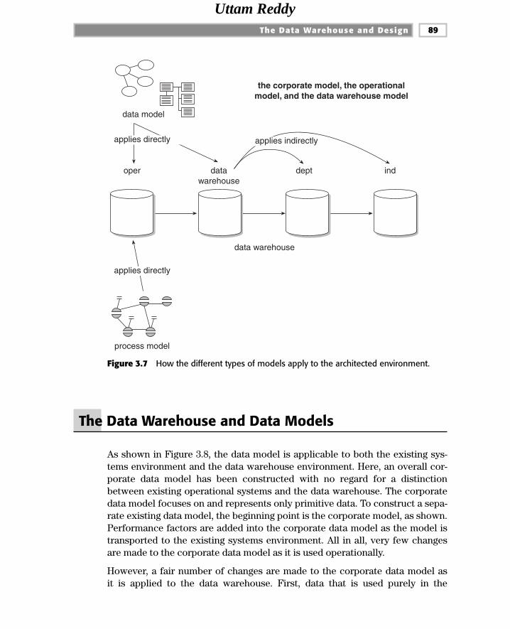
The Data Warehouse and Data Models

As shown in Figure 3.8, the data model is applicable to both the existing sys-tems environment and the data warehouse environment. Here, an overall cor-porate data model has been constructed with no regard for a distinctionbetween existing operational systems and the data warehouse. The corporatedata model focuses on and represents only primitive data. To construct a sepa-rate existing data model, the beginning point is the corporate model, as shown.Performance factors are added into the corporate data model as the model istransported to the existing systems environment. All in all, very few changesare made to the corporate data model as it is used operationally.

However, a fair number of changes are made to the corporate data model asit is applied to the data warehouse. First, data that is used purely in the


the corporate model, the operationalmodel, and the data warehouse model

process model

data model

oper datawarehouse

dept ind

applies directly applies indirectly

data warehouse

applies directly

Figure 3.7 How the different types of models apply to the architected environment.

Uttam Reddy

operational environment is removed. Next, the key structures of the corporatedata model are enhanced with an element of time. Derived data is added to thecorporate data model where the derived data is publicly used and calculatedonce, not repeatedly. Finally, data relationships in the operational environmentare turned into “artifacts” in the data warehouse.

A final design activity in transforming the corporate data model to the datawarehouse data model is to perform “stability” analysis. Stability analysisinvolves grouping attributes of data together based on their propensity forchange. Figure 3.9 illustrates stability analysis for the manufacturing environ-ment. Three tables are created from one large general-purpose table based onthe stability requirements of the data contained in the tables.

In Figure 3.9, data that seldom changes is grouped, data that sometimeschanges is grouped, and data that frequently changes is grouped. The net

C H A P T E R 390

• remove pure operational data

• add element of time to key

• add derived data where appropriate

• create artifacts of relationships

• operational data model equalscorporate data model

• performance factors are added priorto database design

operationaldata model

data model

oper

data warehouse

data warehousedata model

data model

corporatemodel

data model

Figure 3.8 How the different levels of modeling relate.

Uttam Reddy

result of stability analysis (which usually is the last step of data modelingbefore physical database design) is to create groups of data with similarcharacteristics.

There is, then, a common genesis of data models. As an analogy, say the cor-porate data model is Adam, the operational data model is Cain, and the data


part-iddescriptionorder unitlead timeacceptable reject rateshipping manifest. . . . . . . . . . . . . . . . . . . .

part-iddescriptionprimary substituteqty on handorder unitsafety stockprimary supplierlead timeacceptable reject rateexpediterlast order datelast order amountlast delivery toshipping manifestorder amount. . . . . . . . . . . . . . . . . . . .

Part Table SeldomChanges

SometimesChanges

FrequentlyChanges

part-idprimary substitutesafety stockprimary supplierexpediter. . . . . . . . . . . . . . . . . .part-id

qty on handlast order datelast order amountlast delivery toorder amount. . . . . . . . . . . . . . . .

Figure 3.9 An example of stability analysis.

Uttam Reddy

warehouse data model is Abel. They are all from the same lineage, but at thesame time, they are all different.

The Data Warehouse Data Model

(Other books have been written on data modeling, detailing several differentapproaches. Any number can be used successfully in building a data ware-house. The approach summarized here can be further explored in my previousbook Information Systems Architecture: Development in the 90s [QED/Wiley,1992].)

There are three levels of data modeling: high-level modeling (called the ERD,entity relationship level), midlevel modeling (called the data item set, or DIS),and low-level modeling (called the physical model).

The high level of modeling features entities and relationships, as shown in Fig-ure 3.10. The name of the entity is surrounded by an oval. Relationships amongentities are depicted with arrows. The direction and number of the arrowheadsindicate the cardinality of the relationship, and only direct relationships areindicated. In doing so, transitive dependencies are minimized.

The entities that are shown in the ERD level are at the highest level of abstrac-tion. What entities belong in the scope of the model and what entities do not are

C H A P T E R 392

An oval represents an entity, or major subject.

a 1:n relationship

a 1:1 relationship

an m:n relationship

a simple ERD for the manufacturing environmentassembly

part

order

supplier

Figure 3.10 Representing entities and relationships.

Uttam Reddy

determined by what is termed the “scope of integration,” as shown in Fig-ure 3.11. The scope of integration defines the boundaries of the data model andneeds to be defined before the modeling process commences. The scope isagreed on by the modeler, the management, and the ultimate user of the system.If the scope is not predetermined, there is the great chance that the modelingprocess will continue forever. The definition of the scope of integration shouldbe written in no more than five pages and in language understandable to thebusinessperson.

As shown in Figure 3.12, the corporate ERD is a composite of many individualERDs that reflect the different views of people across the corporation. Separate


scope of integration

datamodel

Figure 3.11 The scope of integration determines what portion of the enterprise will bereflected in the data model.

Uttam Reddy

high-level data models have been created for different communities within thecorporation. Collectively, they make up the corporate ERD.

The ERDs representing the known requirements of the DSS community are cre-ated by means of user view sessions, which are interview sessions with theappropriate personnel in the various departments.

The Midlevel Data Model

After the high-level data model is created, the next level is established—themidlevel model, or the DIS. For each major subject area, or entity, identified inthe high-level data model, a midlevel model is created, as seen in Figure 3.13.The high-level data model has identified four entities, or major subject areas.Each area is subsequently developed into its own midlevel model.

Interestingly, only very rarely are all of the midlevel models developed at once.The midlevel data model for one major subject area is expanded, then a portionof the model is fleshed out while other parts remain static, and so forth.

Shown in Figure 3.14, four basic constructs are found at the midlevel model:

C H A P T E R 394

user view (1)

user view (2)

user view (3)

user view (n)

ERD(1)

ERD(2)

ERD(3)

ERD(n)

corporate ERD

Figure 3.12 The construction of the corporate ERD from the different user view ERDs.

Uttam Reddy

■■ A primary grouping of data

■■ A secondary grouping of data

■■ A connector, signifying the relationships of data between major subjectareas

■■ “Type of” data

The primary grouping exists once, and only once, for each major subject area.It holds attributes that exist only once for each major subject area. As with all


the relationship between the ERD and the DIS

DIS

ERD

DIS

DIS

DIS

Figure 3.13 Each entity in the ERD is further defined by its own DIS.

key

connectordata

xxxxxxkey

xxxxxx

xxxxxxkey

xxxxxx

xxxxxxkey

xxxxxx

xxxxxxkey

xxxxxx

xxxxxxkey

xxxxxx

primarygroupingof data

secondarygroupingof data

“type of”data

Figure 3.14 The four constructs that make up the midlevel data model.

Uttam Reddy

groupings of data, the primary grouping contains attributes and keys for eachmajor subject area.

The secondary grouping holds data attributes that can exist multiple times foreach major subject area. This grouping is indicated by a line emanating down-ward from the primary grouping of data. There may be as many secondarygroupings as there are distinct groups of data that can occur multiple times.

The third construct is the connector. The connector relates data from onegrouping to another. A relationship identified at the ERD level results in anacknowledgment at the DIS level. The convention used to indicate a connectoris an underlining of a foreign key.

The fourth construct in the data model is “type of” data. “Type of” data is indi-cated by a line leading to the right of a grouping of data. The grouping of data tothe left is the supertype. The grouping of data to the right is the subtype of data.

These four data modeling constructs are used to identify the attributes of datain a data model and the relationship among those attributes. When a relation-ship is identified at the ERD level, it is manifested by a pair of connector rela-tionships at the DIS level. Figure 3.15 shows one of those pairs.

At the ERD, a relationship between customer and account has been identified.At the DIS level for account, there exists a connector beneath account. Thisindicates that an account may have multiple customers attached to it. Notshown is the corresponding relationship beneath the customer in the customerDIS. Here will be a connector to account, indicating that a customer can havean account or accounts.

C H A P T E R 396

acctno balance domicile date opened

address street city state zip

customerERD

customer

account

Figure 3.15 The relationships identified in the ERD are reflected by connectors in theDIS. Note that only one connector—from acctno to customer—is shown inthis diagram. In reality, another connector from customer to acctno wouldbe shown elsewhere in the DIS for customer.

Uttam Reddy

Figure 3.16 shows what a full-blown DIS might look like, where a DIS exists foran account for a financial institution. In this example, all of the different con-structs are shown in the DIS.

Of particular interest is the case where a grouping of data has two “type of”lines emanating from it, as seen in Figure 3.17. The two lines leading to the rightindicate that there are two “type of” criteria. One type of criteria is by activitytype—either a deposit or a withdrawal. The other line indicates another—either an ATM activity or a teller activity. Collectively, the two types of activityencompass the following transactions:

■■ ATM deposit

■■ ATM withdrawal

■■ Teller deposit

■■ Teller withdrawal

Another feature of the diagram is that all common data is to the left and allunique data is to the right. For example, the attributes date and time are com-mon to all transactions, but cashbox balance relates only to teller activity.

The relationship between the data model and the physical tables that resultfrom the data model is shown in Figure 3.18. In general, each grouping of dataresults in a table being defined in the database design process. Assuming that to


acctno balance domicile date opened

address street city state zip

customer

Loansacctno credit limit interest type

savingsacct no minimum deposit minimum balance

trustacctno officer category

collateral

non-collateral

Home

addresscosignerappraisal

caryearmakemodelcolor

bankcard

acctno type limit exp date

signature

Figure 3.16 An expanded DIS showing the different types of loans that a bank may support.

Uttam Reddy

be the case, two transactions result in several table entries, as seen in the Fig-ure 3.18. The physical table entries that resulted came from the following twotransactions:

■■ An ATM withdrawal that occurred at 1:31 P.M. on January 2

■■ A teller deposit that occurred at 3:15 P.M. on January 5

The two transactions caused six entries in five separate tables to be generated.

Like the corporate ERD that is created from different ERDs reflecting the com-munity of users, the corporate DIS is created from multiple DISs, as illustratedby Figure 3.19. When the interviews or JAD sessions are done for a particularuser, a DIS, as well as an ERD, is created. The parochial DIS is then merged withall other DISs to form the corporate view of a DIS.

The Physical Data Model

The physical data model is created from the midlevel data model merely byextending the midlevel data model to include keys and physical characteristicsof the model. At this point, the physical data model looks like a series of tables,sometimes called relational tables.

C H A P T E R 398

Banking activity

acctnodatetimeamountlocationtypeteller

Deposit

instrumentposting requested?

withdrawal

balance verified?ID used?cash/check/other?

ATM

ID numberlimit request exceededexact time stamp

teller

teller IDautomated verificationsequence numbercashbox balance

the types of activityrepresented by this DIS:

• ATM deposit• ATM withdrawal• teller deposit• teller withdrawal

Figure 3.17 A DIS showing different subcategorization criteria.

TEAMFLY

Team-Fly®

Uttam Reddy

Although it is tempting to say that the tables are ready to be cast into the con-crete of physical database design, one last design step remains—factoring inthe performance characteristics. With the data warehouse, the first step indoing so is deciding on the granularity and partitioning of the data. This is cru-cial. (Of course, the key structure is changed to add the element of time, towhich each unit of data is relevant.)

After granularity and partitioning are factored in, a variety of other physicaldesign activities are embedded into the design, as outlined in Figure 3.20. At theheart of the physical design considerations is the usage of physical I/O(input/output). Physical I/O is the activity that brings data into the computer


ATM

ID numberlimit request exceededexact time stamp

withdrawal

balance verified?ID used?cash/check/other?

deposit

instrumentposting requested?

the different types of data that would exist in separate tables as a result of the DIS

bankingactivity

acct = 1234date = Jan 2time = 1:31 pmamount = $25type = w/dteller = atm

acct = 1234date = Jan 5time = 3:15 pmamount = $1000type = depositteller = teller

bankingactivity table

deposit table

acct = 1234date = Jan 5time = 3:15 pminstrument = checkposting requested = no

withdrawal table

acct = 1234date = Jan 2time = 1:31 pmbalance verified = yesID used = yescheck

ATM table

acct = 1234date = Jan 2time = 1:31 pmID number = Ab00191Slimit exceeded = noexact timestamp = 1:31:35:05

teller table

acct = 1234date = Jan 5time = 3:15 pmteller ID = JLCautomated verification = nosequence number = 901cashbox balance = $112,109.32

acctnodatetimeamountlocationtypeteller

teller

teller IDautomated verificationsequence numbercashbox balance

Figure 3.18 The table entries represented by the two transactions.

Uttam Reddy

from storage or sends data to storage from the computer. Figure 3.21 shows asimple case of I/O.

Data is transferred to and from the computer to storage in blocks. The I/O eventis vital to performance because the transfer of data to and from storage to thecomputer occurs roughly two to three orders of magnitude slower than thespeeds at which the computer runs. The computer runs internally in terms ofnanosecond speed. Transfer of data to and from storage occurs in terms of mil-liseconds. Thus, physical I/O is the main impediment to performance.

C H A P T E R 3100

user view (1)

user view (2)

user view (3)

user view (n)

corporate DIS

corporate ERD

ERD(2)

DIS(2)

ERD(1)DIS(1)

ERD(3)

DIS(3)

ERD(n)

DIS(n)

Figure 3.19 The corporate DIS is made up of the DIS created as a result of each userview session.

Uttam Reddy

The job of the data warehouse designer is to organize data physically for thereturn of the maximum number of records from the execution of a physical I/O.(Note: This is not an issue of blindly transferring a large number of recordsfrom DASD to main storage; instead, it is a more sophisticated issue of trans-ferring a bulk of records that have a high probability of being accessed.)

For example, suppose a programmer must fetch five records. If those recordsare organized into different blocks of data on storage, then five I/Os will berequired. But if the designer can anticipate that the records will be needed as agroup and can physically juxtapose those records into the same block, thenonly one I/O will be required, thus making the program run much moreefficiently.

There is another mitigating factor regarding physical placement of data in thedata warehouse: Data in the warehouse normally is not updated. This frees thedesigner to use physical design techniques that otherwise would not be accept-able if it were regularly updated.


physicaldatabase design

• performance– arrays of data– merging tables– selective redundancy– further separation of data– derived data– preformatting, preallocation– relationship artifacts– prejoining tables

data model

Figure 3.20 Getting good performance out of the data warehouse environment.

computer

I/O

Figure 3.21 Getting the most out of the physical I/Os that have to be done.

Uttam Reddy

The Data Model and Iterative Development

In all cases, the data warehouse is best built iteratively. The following are someof the many reasons why iterative development is important:

■■ The industry track record of success strongly suggests it.

■■ The end user is unable to articulate requirements until the first iteration isdone.

■■ Management will not make a full commitment until actual results are tangi-ble and obvious.

■■ Visible results must be seen quickly.

What may not be obvious is the role of the data model in iterative development.To understand the role of the data model during this type of development, con-sider the typical iterative development suggested by Figure 3.22. First, onedevelopment effort is undertaken, then another, and so forth. The data ware-house serves as a roadmap for each of the development efforts, as seen in Fig-ure 3.23.

When the second development effort ensues, the developer is confident that heor she will intersect his or her effort with the first development effort becauseall development efforts are being driven from the data model. Each succeedingdevelopment effort builds on the preceding one. The result is that the differentdevelopment efforts are done under a unifying data model. And because theyare built under a single data model, the individual iterative efforts produce acohesive and tightly orchestrated whole, as seen in Figure 3.24.

When the different iterations of development are done with no unifying datamodel, there is much overlap of effort and much separate, disjoint develop-ment. Figure 3.25 suggests this cacophonous result.

There is, then, an indirect, yet important, correlation between the data modeland the ability to achieve long-term integration and a harmonious effort in theincremental and iterative development of a data warehouse.

Normalization/Denormalization

The output of the data model process is a series of tables, each of which con-tains keys and attributes. The normal output produces numerous table, each

C H A P T E R 3102

Uttam Reddy


iteration a

iteration b

iteration c

iteration d

Figure 3.22 The different iterations of data warehouse development.

iteration a

iteration b

iteration c

iteration d

Figure 3.23 The data model allows the different iterations of development to be built ina cohesive manner.

Figure 3.24 At the end of the development effort, all the iterations fit together.

Uttam Reddy

with only a modicum of data. While there is nothing wrong—per se—with lotsof little tables, there is a problem from a performance perspective. Consider thework the program has to do in order to interconnect the tables dynamically, asshown in Figure 3.26.

In Figure 3.26, a program goes into execution. First, one table is accessed, thenanother. To execute successfully, the program must jump around many tables.Each time the program jumps from one table to the next, I/O is consumed, interms of both accessing the data and accessing the index to find the data. If onlyone or two programs had to pay the price of I/O, there would be no problem.But when all programs must pay a stiff price for I/O, performance in generalsuffers, and that is precisely what happens when many small tables, each con-taining a limited amount of data, are created as a physical design.

A more rational approach is to physically merge the tables so that minimal I/Ois consumed, as seen in Figure 3.27. Now the same program operates as before,only it needs much less I/O to accomplish the same task.

The question, then, becomes what is a sane strategy to merge the tables so thatthe maximum benefit is derived? It is in answering this question that the physi-cal database designer earns his or her reward.

Merging tables is only one design technique that can save I/O. Another very use-ful technique is creating an array of data. In Figure 3.28, data is normalized sothat each occurrence of a sequence of data resides in a different physical loca-tion. Retrieving each occurrence, n, n � 1, n � 2, . . . , requires a physical I/Oto get the data. If the data were placed in a single row in an array, then a singleI/O would suffice to retrieve it, as shown at the bottom of Figure 3.28.

Of course, it does not make sense to create an array of data in every case. Onlywhen there are a stable number of occurrences, where the data is accessed insequence, where it is created and/or updated in a statistically well-behaved

C H A P T E R 3104

Figure 3.25 When there is no data model, the iterations do not form a cohesive pattern.There is much overlap and lack of uniformity.

Uttam Reddy

sequence, and so forth, does creating an array pay off.

Interestingly, in the data warehouse these circumstances occur regularlybecause of the time-based orientation of the data. Data warehouse data isalways relevant to some moment in time, and units of time occur with great reg-ularity. In the data warehouse, creating an array by month, for example, is avery easy, natural thing to do.

Another important design technique that is especially relevant to the data ware-house environment is the deliberate introduction of redundant data. Figure 3.29


program

Figure 3.26 When there are many tables, much I/O is required for dynamic intercon-nectability.

program

Figure 3.27 When tables are physically merged, much less I/O is required.

Uttam Reddy

shows an example where the deliberate introduction of redundant data pays abig dividend. In the top of Figure 3.29, the field—description—is normalizedand exists nonredundantly. In doing so, all processes that must see the descrip-tion of a part must access the base parts table. The access of the data is veryexpensive, although the update of the data is optimal.

In the bottom of Figure 3.29, the data element—description—has been deliber-ately placed in the many tables where it is likely to be used. In doing so, theaccess of data is more efficient, and the update of data is not optimal. For datathat is widely used (such as description), and for data that is stable (such asdescription), however, there is little reason to worry about update. In particular,in the data warehouse environment there is no concern whatsoever for update.

Another useful technique is the further separation of data when there is a widedisparity in the probability of access. Figure 3.30 shows such a case.

In Figure 3.30, concerning a bank account, the domicile of the account and thedata opened for the account are normalized together with the balance of theaccount. Yet the balance of the account has a very different probability ofaccess than the other two data elements. The balance of an account is very pop-ular, while the other data is hardly ever accessed. To make I/O more efficientand to store the data more compactly, it makes sense to further reduce the nor-malized table into two separate tables, as shown.

C H A P T E R 3106

n

n+2

n+4 ......

......

n+3 ...

......

......

.... ....

data physically organized into an array

an array of datascattered overseparate physicalblocks

creating arrays of data for performance

n+1

n n+1 n+2 n+3 n+4

program

program

n

Figure 3.28 Under the right circumstances, creating arrays of data can save consider-able resources.

Uttam Reddy

Occasionally, the introduction of derived (i.e., calculated) data into the physicaldatabase design can reduce the amount of I/O needed. Figure 3.31 shows sucha case. A program accesses payroll data regularly in order to calculate theannual pay and taxes that have been paid. If the program is run regularly and atthe year’s end, it makes sense to create fields of data to store the calculateddata. The data has to be calculated only once. Then all future requirements canaccess the calculated field. This approach has another advantage in that oncethe field is calculated, it will not have to be calculated again, eliminating therisk of faulty algorithms from incorrect evaluations.


access access access access access

bompartno. . . . .. . . . .. . . . .

inventorypartno. . . . .. . . . .

prod ctlpartno. . . . .. . . . .. . . . .

mrppartno. . . . .. . . . .

partno desc u/m qty . . . . .

access access access access accessupdate

Description is nonredundant and is used frequently, but is seldom updated.

bompartno desc . . . . . . . . . .

inventorypartno desc . . . . .

prod ctlpartno desc . . . . . . . . . .

mrppartno desc . . . . .

partno desc u/m qty . . . . .

selective use of redundancy

update

Figure 3.29 Description is redundantly spread over the many places it is used. It mustbe updated in many places when it changes, but it seldom, if ever, does.

Uttam Reddy

One of the most innovative techniques in building a data warehouse is what canbe termed a “creative” index, or a creative profile (a term coined by Les Moore).Figure 3.32 shows an example of a creative index. This type of creative index iscreated as data is passed from the operational environment to the data ware-house environment. Because each unit of data has to be handled in any case, itrequires very little overhead to calculate or create an index at this point.

C H A P T E R 3108

low probabilityof access

very high probabilityof access

acctno domicile date opened balance

acctno domicile date opened

acctno balance

Figure 3.30 Further separation of data based on a wide disparity in the probability ofaccess.

week 1paytaxesFICAother

introducing derived data



.............

.............

.............

.............

.............


annual pay,taxes,FICA,other

program


annual pay,taxes,FICA,other




.............

.............

.............

.............

.............

Figure 3.31 Derived data, calculated once, then forever available.

TEAMFLY

Team-Fly®

Uttam Reddy

The creative index does a profile on items of interest to the end user, such asthe largest purchases, the most inactive accounts, the latest shipments, and soon. If the requirements that might be of interest to management can be antici-pated (admittedly, they cannot in every case), at the time of passing data to thedata warehouse, it makes sense to build a creative index.

A final technique that the data warehouse designer should keep in mind is themanagement of referential integrity. Figure 3.33 shows that referential integrityappears as “artifacts” of relationships in the data warehouse environment.

In the operational environment, referential integrity appears as a dynamic linkamong tables of data. But because of the volume of data in a data warehouse,because the data warehouse is not updated, and because the warehouse repre-sents data over time and relationships do not remain static, a differentapproach should be taken toward referential integrity. In other words, relation-ships of data are represented by an artifact in the data warehouse environment.Therefore, some data will be duplicated, and some data will be deleted when


existing systems

lightly summarized data

true archivalcreative indexes;

profiles

creative indexes/profiles

extract,load

Figure 3.32 Examples of creative indexes:• The top 10 customers in volume are ___.• The average transaction value for this extract was $nnn.nn.• The largest transaction was $nnn.nn.• The number of customers who showed activity without purchasing

was nn.

Uttam Reddy

other data is still in the warehouse. In any case, trying to replicate referentialintegrity in the data warehouse environment is a patently incorrect approach.

Snapshots in the Data Warehouse

Data warehouses are built for a wide variety of applications and users, such ascustomer systems, marketing systems, sales systems, and quality control sys-

C H A P T E R 3110

But, in the data warehouse environment:

• There is much more data than in the operational environment.• Once in the warehouse, the data doesn't change.• There is a need to represent more than one business rule over time.• Data purges in the warehouse are not tightly coordinated.

In operational systems, the relationships between databases arehandled by referential integrity.

data warehouse and referential integrity

Artifacts in the data warehouseenvironment:

• can be managed independently• are very efficient to access• do not require update

a b'

a b'

a b'

a b'subject A subject B

b a'

b a'

b a'

b a'

b a'

b a'

b a'

b a'

Figure 3.33 Referential integrity in the data warehouse environment.

Uttam Reddy

tems. Despite the very diverse applications and types of data warehouses, acommon thread runs through all of them. Internally, each of the data ware-houses centers around a structure of data called a “snapshot.” Figure 3.34shows the basic components of a data warehouse snapshot.

Snapshots are created as a result of some event occurring. Several kinds ofevents can trigger a snapshot. One event is the recording of information abouta discrete activity, such writing a check, placing a phone call, the receipt of ashipment, the completion of an order, or the purchase of a policy. In the case ofa discrete activity, some business occurrence has occurred, and the businessmust make note of it. In general, discrete activities occur randomly.

The other type of snapshot trigger is time, which is a predictable trigger, suchas the end of the day, the end of the week, or the end of the month.

The snapshot triggered by an event has four basic components:

■■ A key

■■ A unit of time

■■ Primary data that relates only to the key

■■ Secondary data captured as part of the snapshot process that has no directrelationship to the primary data or key

Of these components, only secondary data is optional.

The key can be unique or nonunique and it can be a single element of data. In atypical data warehouse, however, the key is a composite made up of many ele-ments of data that serve to identify the primary data. The key identifies therecord and the primary data.

The unit of time, such as year, month, day, hour, and quarter, usually (but notalways) refers to the moment when the event being described by the snapshothas occurred. Occasionally, the unit of time refers to the moment when the cap-ture of data takes place. (In some cases a distinction is made between when an


time

key nonkeyprimary

data

secondary data

Figure 3.34 A data warehouse record of data is a snapshot taken at one moment intime and includes a variety of types of data.

Uttam Reddy

event occurs and when the information about the event is captured. In othercases no distinction is made.) In the case of events triggered by the passage oftime, the time element may be implied rather than directly attached to thesnapshot.

The primary data is the nonkey data that relates directly to the key of therecord. As an example, suppose the key identifies the sale of a product. The ele-ment of time describes when the sale was finalized. The primary data describeswhat product was sold at what price, conditions of the sale, location of the sale,and who were the representative parties.

The secondary data—if it exists—identifies other extraneous information cap-tured at the moment when the snapshot record was created. An example of sec-ondary data that relates to a sale is incidental information about the productbeing sold (such as how much is in stock at the moment of sale). Other sec-ondary information might be the prevailing interest rate for a bank’s preferredcustomers at the moment of sale. Any incidental information can be added to adata warehouse record, if it appears at a later time that the information can beused for DSS processing. Note that the incidental information added to thesnapshot may or may not be a foreign key. A foreign key is an attribute found ina table that is a reference to the key value of another table where there is a busi-ness relationship between the data found in the two tables.

Once the secondary information is added to the snapshot, a relationshipbetween the primary and secondary information can be inferred, as shown inFigure 3.35. The snapshot implies that there is a relationship between sec-ondary and primary data. Nothing other than the existence of the relationshipis implied, and the relationship is implied only as of the instant of the snapshot.Nevertheless, by the juxtaposition of secondary and primary data in a snapshotrecord, at the instant the snapshot was taken, there is an inferred relationshipof data. Sometimes this inferred relationship is called an “artifact.” The snap-shot record that has been described is the most general and most widely foundcase of a record in a data warehouse.

C H A P T E R 3112

nonkeyprimary data

secondarydata

Figure 3.35 The artifacts of a relationship are captured as a result of the implied rela-tionship of secondary data residing in the same snapshot as primary data.

Uttam Reddy

Meta Data

An important component of the data warehouse environment is meta data.Meta data, or data about data, has been a part of the information processingmilieu for as long as there have been programs and data. But in the world ofdata warehouses, meta data takes on a new level of importance, for it affordsthe most effective use of the data warehouse. Meta data allows the enduser/DSS analyst to navigate through the possibilities. Put differently, when auser approaches a data warehouse where there is no meta data, the user doesnot know where to begin the analysis. The user must poke and probe the datawarehouse to find out what data is there and what data is not there and consid-erable time is wasted. Even after the user pokes around, there is no guaranteethat he or she will find the right data or correctly interpret the data encoun-tered. With the help of meta data, however, the end user can quickly go to thenecessary data or determine that it isn’t there.

Meta data then acts like an index to the contents of the data warehouse. It sitsabove the warehouse and keeps track of what is where in the warehouse. Typi-cally, items the meta data store tracks are as follows:

■■ Structure of data as known to the programmer

■■ Structure of data as known to the DSS analyst

■■ Source data feeding the data warehouse

■■ Transformation of data as it passes into the data warehouse

■■ Data model

■■ Relationship between the data model and the data warehouse

■■ History of extracts

Managing Reference Tables in a Data Warehouse

When most people think of data warehousing, their thoughts turn to the nor-mal, large databases constantly being used by organizations to run day-to-daybusiness such as customer files, sales files, and so forth. Indeed, these commonfiles form the backbone of the data warehousing effort. Yet another type of databelongs in the data warehouse and is often ignored: reference data.

Reference tables are often taken for granted, and that creates a special prob-lem. For example, suppose in 1995 a company has some reference tables andstarts to create its data warehouse. Time passes, and much data is loaded into


Uttam Reddy

the data warehouse. In the meantime, the reference table is used operationallyand occasionally changes. In 1999, the company needs to consult the referencetable. A reference is made from 1995 data to the reference table. But the refer-ence table has not been kept historically accurate, and the reference from 1995data warehouse data to reference entries accurate as of 1999 produces veryinaccurate results. For this reason, reference data should be made time-variant,just like all other parts of the data warehouse.

Reference data is particularly applicable to the data warehouse environmentbecause it helps reduce the volume of data significantly. There are many designtechniques for the management of reference data. Two techniques—at theopposite ends of the spectrum—are discussed here. In addition, there are manyvariations on these options.

Figure 3.36 shows the first design option, where a snapshot of an entire refer-ence table is taken every six months This approach is quite simple and at firstglance appears to make sense. But the approach is logically incomplete. Forexample, suppose some activity had occurred to the reference table on March15. Say a new entry—ddw—was added, then on May 10 the entry for ddw wasdeleted. Taking a snapshot every six months would not capture the activity thattranspired from March 15 to May 10.

A second approach is shown in Figure 3.37. At some starting point a snapshot ismade of a reference table. Throughout the year, all the activities against the ref-erence table are collected. To determine the status of a given entry to the refer-ence table at a moment in time, the activity is reconstituted against thereference table. In such a manner, logical completeness of the table can bereconstructed for any moment in time. Such a reconstruction, however, is a nota trivial matter; it may represent a very large and complex task.

The two approaches outlined here are opposite in intent. The first approach issimple but logically incomplete. The second approach is very complex but log-ically complete. Many design alternatives lie between these two extremes.However they are designed and implemented, reference tables need to be man-aged as a regular part of the data warehouse environment.

C H A P T E R 3114

Jan 1 AAA - Amber Auto AAT - Allison's AAZ - AutoZone BAE - Brit Eng ................

July 1 AAA - Amber Auto AAR - Ark Electric BAE - Brit Eng BAG - Bill's Garage ...................

Jan 1 AAA - Alaska Alt AAG - German Air AAR - Ark Electric BAE - Brit Eng ..................

Figure 3.36 A snapshot is taken of a reference table in its entirety every six months—oneapproach to the management of reference tables in the data warehouse.

Uttam Reddy

Cyclicity of Data—The Wrinkle of Time

One of the intriguing issues of data warehouse design is the cyclicity of data, orthe length of time a change of data in the operational environment takes to bereflected in the data warehouse. Consider the data in Figure 3.38.

The current information is shown for Judy Jones. The data warehouse containsthe historical information about Judy. Now suppose Judy changes addresses.Figure 3.39 shows that as soon as that change is discovered, it is reflected in theoperational environment as quickly as possible.

Once the data is reflected in the operational environment, the changes need tobe moved to the data warehouse. Figure 3.40 shows that the data warehousehas a correction to the ending date of the most current record and a new recordhas been inserted reflecting the change.

The issue is, how soon should this adjustment to the data warehouse data bemade? As a rule, at least 24 hours should pass from the time the change isknown to the operational environment until the change is reflected into thedata warehouse (see Figure 3.41). There should be no rush to try to move thechange into the data warehouse as quickly as possible. This “wrinkle of time”should be implemented for several reasons.

The first reason is that the more tightly the operational environment is coupledto the data warehouse, the more expensive and complex the technology is. A24-hour wrinkle of time can easily be accomplished with conventional technol-ogy. A 12-hour wrinkle of time can be accomplished but at a greater cost oftechnology. A 6-hour wrinkle of time can be accomplished but at an evengreater cost in technology.


Jan 1 - add TWQ - Taiwan DairyJan 16 - delete AATFeb 3 - add AAG - German PowerFeb 27 - change GYY - German Govt........................................................................

A complete snapshot is takenon the first of the year.

Changes to the reference table arecollected throughout the year and areable to be used to reconstruct the tableat any moment in time.

Jan 1 AAA - Amber Auto AAT - Allison's AAZ - AutoZone BAE - Brit Eng ................. ..................

Figure 3.37 Another approach to the management of reference data.

Uttam Reddy

C H A P T E R 3116

Rte 4, Austin, TX

operational

J Jones has movedto Rte 4, Austin, TX

J Jones123 MainCredit - AA

Figure 3.39 The first step is to change the operational address of J Jones.

operational


J Jones1989-1990Apt BCredit - B

J Jones1990-1991Apt BCredit - AA

J Jones1992-present123 MainCredit - AA

J Jones123 MainCredit - AA

datawarehouse

Figure 3.38 What happens when the corporation finds out that J Jones has moved?

Uttam Reddy


change theending date


J Jones1989-1990Apt BCredit - B

J Jones1990-1991Apt BCredit - AA

datawarehouse

J Jones1992-present123 MainCredit - AA

1993

insertJ Jones1993-presentRte 4, Austin, TXCredit - AA

Figure 3.40 The activities that occur in the data warehouse as a result of the change of address.

operational

24-hour delay

data warehouse

change change

“wrinkle of time”

Figure 3.41 There needs to be at least a 24-hour lag—a “wrinkle of time”—between thetime a change is known to the operational environment and the time whenthe change is reflected into the data warehouse.

Uttam Reddy

A more powerful reason for the wrinkle of time is that it imposes a certain dis-cipline on the environments. With a 24-hour wrinkle there is no temptation todo operational processing in the data warehouse and data warehouse process-ing in the operational environment. But if the wrinkle of time is reduced—say,to 4 hours—there is the temptation to do such processing, and that is patentlya mistake.

Another benefit of the wrinkle of time is opportunity for data to settle before itis moved to the data warehouse. Adjustments can be made in the operationalenvironment before the data is sent to the data warehouse. If data is quicklysent to the warehouse and then it is discovered that adjustments must be made,those adjustments need to be made in both the operational environment andthe data warehouse environment.

Complexity of Transformation and Integration

At first glance, when data is moved from the legacy environment to the datawarehouse environment, it appears that nothing more is going on than simpleextraction of data from one place to the next. Because of the deceptive sim-plicity, many organizations start to build their data warehouses manually. Theprogrammer looks at the movement of data from the old operational environ-ment to the new data warehouse environment and declares “I can do that!” Withpencil and coding pad in hand, the programmer anxiously jumps into the cre-ation of code within the first three minutes of the design and development ofthe data warehouse.

First impressions, though, can be very deceiving. What at first appears to benothing more than the movement of data from one place to another quicklyturns into a large and complex task—far larger and more complex than the pro-grammer thought.

Precisely what kind of functionality is required as data passes from the opera-tional, legacy environment to the data warehouse environment? The followinglists some of the necessary functionality:

■■ The extraction of data from the operational environment to the data ware-house environment requires a change in technology. This normallyincludes reading the operational DBMS technology, such as IMS, and writ-ing the data out in newer, data warehouse DBMS technology, such asInformix. There is a need for a technology shift as the data is being moved.And the technology shift is not just one of a changing DBMS. The operatingsystem changes, the hardware changes, and even the hardware-basedstructure of the data changes.

C H A P T E R 3118

TEAMFLY

Team-Fly®

Uttam Reddy

■■ The selection of data from the operational environment may be very com-plex. To qualify a record for extraction processing, several coordinatedlookups to other records in a variety of other files may be necessary,requiring keyed reads, connecting logic, and so on. In some cases, theextraneous data cannot be read in anything but the online environment.When this is the case, extraction of data for the data warehouse mustoccur in the online operating window, a circumstance to be avoided if at allpossible.

■■ Operational input keys usually need to be restructured and convertedbefore they are written out to the data warehouse. Very seldom does aninput key remain unaltered as it is read in the operational environment andwritten out to the data warehouse environment. In simple cases, an ele-ment of time is added to the output key structure. In complex cases, theentire input key must be rehashed or otherwise restructured.

■■ Nonkey data is reformatted as it passes from the operational environmentto the data warehouse environment. As a simple example, input data aboutdate is read as YYYY/MM/DD and is written to the output file asDD/MM/YYYY. (Reformatting of operational data before it is ready to gointo a data warehouse often becomes much more complex than this simpleexample.)

■■ Data is cleansed as it passes from the operational environment to the datawarehouse environment. In some cases, a simple algorithm is applied toinput data in order to make it correct. In complex cases, artificial intelli-gence subroutines are invoked to scrub input data into an acceptable out-put form. There are many forms of data cleansing, including domainchecking, cross-record verification, and simple formatting verification.

■■ Multiple input sources of data exist and must be merged as they pass intothe data warehouse. Under one set of conditions the source of a data ware-house data element is one file, and under another set of conditions thesource of data for the data warehouse is another file. Logic must be spelledout to have the appropriate source of data contribute its data under theright set of conditions.

■■ When there are multiple input files, key resolution must be done before thefiles can be merged. This means that if different key structures are used inthe different input files, the merging program must have the logic embed-ded that allows resolution.

■■ With multiple input files, the sequence of the files may not be the same oreven compatible. In this case, the input files need resequenced. This is nota problem unless many records must be resequenced, which unfortunatelyis almost always the case.


Uttam Reddy

■■ Multiple outputs may result. Data may be produced at different levels ofsummarization by the same data warehouse creation program.

■■ Default values must be supplied. Under some conditions an output value inthe data warehouse will have no source of data. In this case, the defaultvalue to be used must be specified.

■■ The efficiency of selection of input data for extraction often becomes areal issue. Consider the case where at the moment of refreshment there isno way to distinguish operational data that needs to be extracted fromoperational data that does not need to be extracted. When this occurs, theentire operational file must be read. Reading the entire file is especiallyinefficient because only a fraction of the records is actually needed. Thistype of processing causes the online environment to be active, which fur-ther squeezes other processing in the online environment.

■■ Summarization of data is often required. Multiple operational input recordsare combined into a single “profile” data warehouse record. To do summa-rization, the detailed input records to be summarized must be properlysequenced. In the case where different record types contribute to the sin-gle summarized data warehouse record, the arrival of the different inputrecord types must be coordinated so that a single record is produced.

■■ Renaming of data elements as they are moved from the operational envi-ronment to the data warehouse must be tracked. As a data element movesfrom the operational environment to the data warehouse environment, itusually changes its name. Documentation of that change must be made.

■■ The input records that must be read have exotic or nonstandard formats.There are a whole host of input types that must be read, then converted onentry into the data warehouse:

■■ Fixed-length records

■■ Variable-length records

■■ Occurs depending on

■■ Occurs clause

Conversion must be made. But the logic of conversion must be specified,and the mechanics of conversion (what the “before” and “after” look like)can be quite complex. In some cases, conversion logic becomes verytwisted.

■■ Perhaps the worst of all: Data relationships that have been built into oldlegacy program logic must be understood and unraveled before those filescan be used as input. These relationships are often Byzantine, arcane, andundocumented. But they must patiently be unwound and deciphered as thedata moves into the data warehouse. This is especially difficult when there

C H A P T E R 3120

Uttam Reddy

is no documentation or when the documentation that exists is out-of-date.And, unfortunately, on many operational legacy systems, there is no docu-mentation. There is an old saying: Real programmers don’t do documenta-tion.

■■ Data format conversion must be done. EBCDIC to ASCII (or vice versa)must be spelled out.

■■ Massive volumes of input must be accounted for. Where there is only asmall amount of data being entered as input, many design options can beaccommodated. But where many records are being input, special designoptions (such as parallel loads and parallel reads) may have to be used.

■■ The design of the data warehouse must conform to a corporate datamodel. As such, there is order and discipline to the design and structuringof the data warehouse. The input to the data warehouse conforms todesign specifications of an application that was written a long time ago.The business conditions behind the application have probably changed 10times since the application was originally written. Much undocumentedmaintenance was done to the application code. In addition, the applicationprobably had no integration requirements to fit with other applications. Allof these mismatches must be accounted for in the design and building ofthe data warehouse.

■■ The data warehouse reflects the historical need for information, while theoperational environment focuses on the immediate, current need for infor-mation. This means that an element of time may need to be added as thedata moves from the operational environment to the data warehouseenvironment.

■■ The data warehouse addresses the informational needs of the corporation,while the operational environment addresses the up-to-the-second clericalneeds of the corporation.

■■ Transmission of the newly created output file that will go into the datawarehouse must be accounted for. In some cases, this is very easy to do; inother cases, it is not simple at all, especially when operating systems arecrossed. Another issue is the location where the transformation will takeplace. Will the transformation take place on the machine hosting the opera-tional environment? Or will raw data be transmitted and the transforma-tion take place on the machine hosting the data warehouse?

And there is more. This list is merely a sampling of the complexities facing theprogrammer when setting off to load the data warehouse.

In the early days of data warehouse, there was no choice but to build the pro-grams that did the integration by hand. Programmers using COBOL, C, and


Uttam Reddy

other languages wrote these. But soon people noticed that these programs weretedious and repetitive. Furthermore, these programs required ongoing mainte-nance. Soon technology appeared that automated the process of integratingdata from the operational environment, called extract/transform/load (ETL)software. The first ETL software was crude, but it quickly matured to the pointwhere almost any transformation could be handled.

ETL software comes in two varieties—software that produces code and soft-ware that produces a runtime module that is parameterized. The code produc-ing software is much more powerful than the runtime software. The codeproducing software can access legacy data in its own format. The runtime soft-ware usually requires that legacy data be flattened. Once flattened, the runtimemodule can read the legacy data. Unfortunately, much intelligence is lost in theflattening of the legacy data.

In any case, ETL software automates the process of converting, reformatting,and integrating data from multiple legacy operational sources. Only under veryunusual circumstances does attempting to build and maintain the opera-tional/data warehouse interface manually make sense.

Triggering the Data Warehouse Record

The basic business interaction that causes the data warehouse to become pop-ulated with data is one that can be called an EVENT/SNAPSHOT interaction. Inthis type of interaction, some event (usually in the operational environment)triggers a snapshot of data, which in turn is moved to the data warehouse envi-ronment. Figure 3.42 symbolically depicts an EVENT/SNAPSHOT interaction.

Events

As mentioned earlier in the chapter, the business event that triggers a snapshotmight be the occurrence of some notable activity, such as the making of a sale,

C H A P T E R 3122

EVENT SNAPSHOT

time nonkey

primary datasecondary

datakey

Figure 3.42 Every snapshot in the data warehouse is triggered by some event.

Uttam Reddy

the stocking of an item, the placing of a phone call, or the delivery of a ship-ment. This type of business event is called an activity-generated event. Theother type of business event that may trigger a snapshot is the marking of theregular passage of time, such as the ending of the day, the ending of the week,or the ending of the month. This type of business event is called a time-gener-ated event.

Whereas events caused by business activities are random, events triggered bythe passage of time are not. The time-related snapshots are created quite regu-larly and predictably.

Components of the Snapshot

Mentioned earlier in this chapter, the snapshot placed in the data warehousenormally contains several components. One component is the unit of time thatmarks the occurrence of the event. Usually (not necessarily always) the unit oftime marks the moment of the taking of the snapshot. The next component ofthe snapshot is the key that identifies the snapshot. The third normal compo-nent of a data warehouse snapshot is the primary, nonkey data that relates tothe key. Finally, an optional component of a snapshot is secondary data that hasbeen incidentally captured as of the moment of the taking of the snapshot andplaced in the snapshot. As mentioned, sometimes this secondary data is calledan artifact of the relationship.

In the simplest case in a data warehouse, each operational activity important tothe corporation will trigger a snapshot. In this case, there is a one-to-one corre-spondence between the business activities that have occurred and the numberof snapshots that are placed in the data warehouse. When there is a one-to-onecorrespondence between the activities in the operational environment and thesnapshots in the data warehouse, the data warehouse tracks the history of allthe activity relating to a subject area.

Some Examples

An example of a simple snapshot being taken every time there is an operational,business activity might be found in a customer file. Every time a customermoves, changes phone numbers, or changes jobs, the data warehouse isalerted, and a continuous record of the history of the customer is made. Onerecord tracks the customer from 1989 to 1991. The next record tracks the cus-tomer from 1991 to 1993. The next record tracks the customer from 1993 to thepresent. Each activity of the customer results in a new snapshot being placed inthe data warehouse.


Uttam Reddy

As another example, consider the premium payments on an insurance policy.Suppose premiums are paid semiannually. Every six months a snapshot recordis created in the data warehouse describing the payment of the premium—when it was paid, how much, and so on.

Where there is little volume of data, where the data is stable (i.e., the datachanges infrequently), and where there is a need for meticulous historicaldetail, the data warehouse can be used to track each occurrence of a businessevent by storing the details of every activity.

Profile Records

But there are many cases in which data in the data warehouse does not meetthese criteria. In some cases, there will be massive volumes of data. In othercases, the content of data changes frequently. And in still other cases, there isno business need for meticulous historical detail of data. When one or more ofthese conditions prevail, a different kind of data warehouse record, called aprofile or an aggregate record, can be created. A profile record groups many dif-ferent, detailed occurrences of operational data into a single record. The singleprofile record represents the many operational records in aggregation.

Profile records represent snapshots of data, just like individual activity records.The difference between the two is that individual activity records in the datawarehouse represent a single event, while profile records in the data ware-house represent multiple events.

Like individual activity records, profile records are triggered by some event-either a business activity or the marking of the regular passage of time. Fig-ure 3.43 shows how an event causes the creation of a profile record.

A profile record is created from the grouping of many detailed records. As anexample, a phone company may at the end of the month take all of a customer’sphone activities for the month and wrap those activities into a single customerrecord in the data warehouse. In doing so, a single representative record can becreated for the customer that reflects all his or her monthly activity. Or a bankmay take all the monthly activities of a customer and create an aggregate datawarehouse record that represents all of his or her banking activities for themonth.

The aggregation of operational data into a single data warehouse record maytake many forms; for example:

■■ Values taken from operational data can be summarized.

C H A P T E R 3124

Uttam Reddy

■■ Units of operational data can be tallied, where the total number of units iscaptured.

■■ Units of data can be processed to find the highest, lowest, average, and soforth.

■■ First and last occurrences of data can be trapped.

■■ Data of certain types, falling within the boundaries of several parameters,can be measured.

■■ Data that is effective as of some moment in time can be trapped.

■■ The oldest and the youngest data can be trapped.

The ways to perform representative aggregation of operational data are limit-less.

Another very appealing benefit to the creation of profile records is organizingthe data in a compact and convenient form for the end user to access and ana-lyze. Done properly, the end user is quite comfortable with the distillation ofmany records into a single record because he or she has to look only in a singleplace to find what is needed. By prepackaging the data into an aggregate recordin the data warehouse, the data architect saves the end user from tediousprocessing.


......

......

...

call 1

call 2

call 3

call 4

call n

customer

The monthly call records areaggregated in order to provide asingle composite record.

Customer/month..........................................

operational

data warehouse

Figure 3.43 The creation of a profile record from a series of detailed records.

Uttam Reddy

Managing Volume

In many cases, the volume of data to be managed in the data warehouse is a sig-nificant issue. Creating profile records is an effective technique for managingthe volume of data. The reduction of the volume of data possible in movingdetailed records in the operational environment into a profile record is remark-able. It is possible (indeed, normal) to achieve a 2-to-3 order-of-magnitudereduction of data by the creation of profile records in a data warehouse.Because of this benefit, the ability to create profile records is a powerful onethat should be in the portfolio of every data architect.

There is, however, a downside to profiling records in the data warehouse.Whenever the use of the profile technique is contemplated, note that a certaincapability or functionality of the data warehouse is lost. Of necessity, detail islost whenever aggregation is done. Keep in mind, however, that losing detail isnot necessarily a bad thing. The designer of the profile record needs to ensurethat the lost detail is not important to the DSS analyst who will ultimately beusing the data warehouse. The data architect’s first line of defense (and easilythe most effective one) is to ensure that such detail is not terribly important isto build the profile records iteratively. By doing so, the data architect has themaneuverability to make changes gracefully. The first iteration of the design ofthe contents of the profile record suggests the second iteration of design, andso forth. As long as the iterations of data warehouse development are small andfast, there is little danger the end user will find many important requirementsleft out of the profile record. The danger comes when profile records are cre-ated and the first iteration of development is large. In this case, the data archi-tect probably will paint himself or herself into a nasty corner becauseimportant detail will have been omitted.

A second approach (which can be used in conjunction with the iterativeapproach) to ensure that important detail is not permanently lost is to create analternative level of historical detail along with the profile record, as shown inFigure 3.44. The alternative detail is not designed to be used frequently; it isstored on slow, inexpensive, sequential storage and is difficult to get to andawkward to work with. But the detail is there should it be needed. When man-agement states that they must have a certain detail, however arcane, it canalways be retrieved, albeit at a cost of time and money.

C H A P T E R 3126

Uttam Reddy

Creating Multiple Profile Records

Multiple profile records can be created from the same detail. In the case of aphone company, individual call records can be used to create a customer pro-file record, a district traffic profile record, a line analysis profile record, and soforth.

The profile records can be used to go into the data warehouse or a data martthat is fed by the data warehouse. When the profile records go into a data ware-house, they are for general-purpose use. When the profile records go into thedata mart, they are customized for the department that uses the data mart.

The aggregation of the operational records into a profile record is almostalways done on the operational server because this server is large enough tomanage volumes of data and because that is where the data resides in any case.Usually creating the profile record involves sorting and merging data. Once theprocess of creating the snapshot becomes complicated and drawn out, whetherthe snapshot should be taken at all becomes questionable.

The meta data records written for profile records are very similar to the metadata records written for single activity snapshots with the exception that theprocess of aggregating the records becomes an important piece of meta data.(Technically speaking, the record of the process of aggregation is “metaprocess” information, not “meta data” information.)


EIS

DSSstandard DSSprocessing

reporting done onan exception basis

operationaldata

profiledata

detailedarchivaldata

Figure 3.44 An alternative to the classical data warehouse architecture—all the detailthat is needed is available while good performance for most DSS process-ing is the norm.

Uttam Reddy

Going from the Data Warehouse to the Operational Environment

The operational environment and the data warehouse environment are about asdifferent as any two environments can be in terms of content, technology,usage, communities served, and a hundred other ways. The interface betweenthe two environments is well documented. Data undergoes a fundamentaltransformation as it passes from the operational environment to the data ware-house environment. For a variety of reasons—the sequence in which businessis conducted, the high performance needs of operational processing, the agingof data, the strong application orientation of operational processing, and soforth—the flow of data from the operational environment to the data ware-house environment is natural and normal. This normal flow of data is shown inFigure 3.45.

The question occasionally arises, is it possible for data to pass from the datawarehouse environment to the operational environment? In other words, candata pass in a reverse direction from that normally experienced? From thestandpoint of technology, the answer certainly is yes, such a passage of data istechnologically possible. Although it is not normal, there are a few isolated cir-cumstances in which data does indeed flow “backward.”

C H A P T E R 3128

legacy applications

datawarehouse

Figure 3.45 The normal flow of data in the legacy application/data warehouse archi-tected environment.

TEAMFLY

Team-Fly®

Uttam Reddy

Direct Access of Data Warehouse Data

Figure 3.46 illustrates the dynamics of the simplest of those circumstances-thedirect access of data from the data warehouse by the operational environment.A request has been made within the operational environment for data thatresides in the data warehouse. The request is transferred to the data warehouseenvironment, and the data is located and transferred to the operational envi-ronment. Apparently, from the standpoint of dynamics, the transfer could notbe easier.

There are a number of serious and uncompromising limitations to the scenarioof the direct access of data in the data warehouse. Some of these are as follows:

■■ The request must be a casual one in terms of response time. It may take aslong as 24 hours for it to be satisfied. This means that the operational pro-cessing that requires the data warehouse data is decidedly not of an onlinenature.

■■ The request for data must be for a minimal amount of data. The data beingtransferred is measured in terms of bytes, not megabytes or gigabytes.

■■ The technology managing the data warehouse must be compatible with thetechnology managing the operational environment in terms of capacity,protocol, and so on.

■■ The formatting of data after it is retrieved from the data warehouse inpreparation for transport to the operational environment must be nonexis-tent (or minimal).


legacy application

results of query

datawarehouse

query

Figure 3.46 A direct query against the data warehouse from the legacy applicationsenvironment.

Uttam Reddy

These conditions preclude most data ever being directly transferred from thedata warehouse to the operational environment. It is easy to see why there is aminimal amount of backward flow of data in the case of direct access.

Indirect Access of Data Warehouse Data

Because of the severe and uncompromising conditions of transfer, directaccess of data warehouse data by the operational environment is a rare occur-rence. Indirect access of data warehouse data is another matter entirely.Indeed, one of the most effective uses of the data warehouse is the indirectaccess of data warehouse data by the operational environment. Some examplesof indirect access of data warehouse data follow.

An Airline Commission Calculation System

One effective indirect use of data warehouse data occurs in the airline environ-ment. Consider, for example, an airline ticketing transaction. A travel agent hascontacted the airline reservation clerk on behalf of a customer. The customerhas requested a ticket for a flight and the travel agent wants to know thefollowing:

■■ Is there a seat available?

■■ What is the cost of the seat?

■■ What is the commission paid to the travel agent?

If the airline pays too much of a commission, it will get the agent’s business, butit will lose money. If the airline pays too little commission, the travel agent will“shop” the ticket and the airline will lose it to another airline that pays a largercommission. It is in the airline’s best interest to calculate the commission itpays very carefully because the calculation has a direct effect on its bottomline.

The interchange between the travel agent and the airline clerk must occur in afairly short amount of time—within two to three minutes. In this two-to-three-minute window the airline clerk must enter and complete several transactions:

■■ Are there any seats available?

■■ Is seating preference available?

■■ What connecting flights are involved?

■■ Can the connections be made?

C H A P T E R 3130

Uttam Reddy

■■ What is the cost of the ticket?

■■ What is the commission?

If the response time of the airline clerk (who is running several transactionswhile carrying on a conversation with the travel agent) starts to be excessive,the airline will find that it is losing business merely because of the poorresponse time. It is in the best interest of the airline to ensure brisk responsetime throughout the dialogue with the travel agent.

The calculation of the optimal commission becomes a critical component of theinterchange. The optimal commission is best calculated by looking at a combi-nation of two factors—current bookings and the load history of the flight. Thecurrent bookings tell how heavily the flight is booked, and the load history yieldsa perspective of how the flight has been booked in the past. Between currentbookings and historical bookings an optimal commission can be calculated.

Though tempting to perform the bookings and flight history calculations online,the amount of data that needs to be manipulated is such that response time suf-fers if they are calculated in this manner. Instead, the calculation of commissionand analysis of flight history are done offline, where there are ample machineresources. Figure 3.47 shows the dynamics of offline commission calculation.


flightdateaverage booking for date

travel agent

airlinereservation

clerk

historicalbookings

currentbookings

flight statuscalculations

Figure 3.47 The flight status file is created periodically by reading the historical data. Itis then a very quick matter for the airline agent to get current bookings andto compare those bookings against the historical average.

Uttam Reddy

The offline calculation and analysis are done periodically, and a small, easy-to-access flight status table is created. When the airline clerk has to interact withthe travel agent, it is an easy matter to look at current bookings and the flightstatus table. The result is a very fast and smooth interaction with the travelagent and the ability to use the data stored in the data warehouse.

A Retail Personalization System

Another example of the indirect use of data warehouse data in the operationalenvironment occurs in the retail personalization system. In this system, a cus-tomer reads a catalog or other flyer issued by the retailer. The customer isinspired to make a purchase or to at least inquire about the catalog. A phonecall to the retailer ensues.

The interchange is about five to eight minutes long. During this time the retailsales representative has a fair amount of processing to do—identify the cus-tomer, take down the specifics of the order, and so forth. The response time iscritical; otherwise, the customer will lose interest.

While the customer is placing the order or making an inquiry, the retail salesrepresentative finds out some other information relevant to the interchange,such as the following:

■■ The last time the customer made a purchase

■■ The last type of purchase made

■■ The market segment(s) in which the customer belongs

While engaging the customer in conversation, the sales representative sayssuch things as these:

■■ “I see it’s been since February that we last heard from you.”

■■ “How was that blue sweater you purchased?”

■■ “Did the problems you had with the pants get resolved?”

In short, the retail sales representative is able to personalize the conversation.The personalization makes the customer more amenable to purchases.

In addition, the retail sales clerk has market segment information available,such as the following:

■■ Male/female

■■ Professional/other

■■ City/country

■■ Children

C H A P T E R 3132

Uttam Reddy

■■ Ages

■■ Sex

■■ Sports

■■ Fishing

■■ Hunting

■■ Beach

Because the phone call can be personalized and the direct marketing segmentfor a customer is available when the customer calls in, the retail sales repre-sentative is able to ask pointed questions, such as these:

■■ “Did you know we have an unannounced sale on swimsuits?”

■■ “We just got in some Italian sunglasses that I think you might like.”

■■ “The forecasters predict a cold winter for duck hunters. We have a specialon waders right now.”

The customer has already taken the time to make a phone call. The personal-ization of the phone call and the knowledge of what products the customer isinterested in give the retailer a very good chance at raising revenue with no fur-ther outlay of cash or advertising. The personalization of the phone call isachieved by the indirect use of the data warehouse. Figure 3.48 shows thedynamics of how personalization is achieved.

In the background (i.e., in the data warehouse environment), an analysis pro-gram is constantly reading and analyzing customer records. This program scansand analyzes historical customer data in a very sophisticated manner. Periodi-cally, the analysis program spins off a file to the operational environment thatcontains such information as the following:

■■ Last purchase date

■■ Last purchase type

■■ Market analysis/segmenting

When the customer rings in, the online prepared file is waiting for use by theretail sales representative.

Credit Scoring

Another example of the indirect use of a data warehouse in the operationalenvironment is credit scoring in the banking/finance environment. Credit scor-ing refers to qualifying (or not qualifying) a person for a loan. Say, for example,a customer walks up to the teller’s window and asks for a loan. The teller takes


Uttam Reddy

in some basic information about the customer and decides whether the loanshould be approved. The interchange occurs in a very short amount of time—5to 10 minutes.

To determine whether the loan should be approved, a certain amount of pro-cessing must be performed. The loan request is first put through a simplescreening process. If the loan is for a small enough amount and if the personhas a stable financial background, then it may be approved with no further pro-cessing. If the loan is for a fair amount and/or the customer does not have a sta-ble, predictable background, then a further check is required.

The background check relies on the data warehouse. In truth, the check is aneclectic one, in which many aspects of the customer are investigated, such asthe following:

■■ Past payback history

■■ Home/property ownership

■■ Financial management

C H A P T E R 3134

customer history file

customer id• last purchase date• last purchase item• product marketing category

consumer

telemarketer

catalog• customer history• sales history• product history• vendor history

market analysisprograms

Figure 3.48 The customer history is at the disposal of the telemarketer at a moment’snotice.

Uttam Reddy

■■ Net worth

■■ Gross income

■■ Gross expenses

■■ Other intangibles

This extensive background check requires quite a bit of diverse historical data.Completing this part of the loan qualification process requires more than a fewminutes.

To satisfy the most customers in the shortest amount of time, an analysis pro-gram is written. Figure 3.49 shows how the analysis program fits in with theother components of credit scoring. The analysis program is run periodicallyand produces a prequalified file for use in the operational environment. In addi-tion to other data, the prequalified file includes the following:

■■ Customer identification

■■ Approved credit limit

■■ Special approval limit

Now when the customer wishes to apply for and get a loan, in a high-performance,online mode the teller qualifies (or does not qualify) the loan request from the


preapproval /preanalysisprogram

preapprovedcustomer file

• account history

• repayment history

• job history

• salary history

• asset management history

customer teller

$$$$$$$$

Figure 3.49 The preapproved customer credit file is accessible by the bank teller in aninstant.

Uttam Reddy

customer. Only if the customer asks for a loan for an amount greater than thepreapproved limit does there need to be an interaction by a loan officer.

Indirect Use of Data Warehouse Data

There is, then, an emerging pattern to the indirect use of data warehouse data.That pattern is shown in Figure 3.50.

The data warehouse is analyzed periodically by a program that examinesrelevant characteristics and criteria. The analysis then creates a small file inthe online environment that contains succinct information about the busi-ness of the enterprise. The small online file is used quickly and efficiently,fitting in with the style of the other processing that occurs in the operationalenvironment.

Following are a few considerations of the elements of the indirect use of datawarehouse data:

■■ The analysis program:

■■ Has many characteristics of artificial intelligence

■■ Has free rein to run on any data warehouse data that is available

■■ Is run in the background, where processing time is not an issue (or atleast not a large issue)

■■ Is run in harmony with the rate at which data warehouse changes

C H A P T E R 3136

onlineenvironment

datawarehouse

analysis/preparation

program

Figure 3.50 The way that data warehouse data is made available to the online opera-tional environment—indirectly.

Uttam Reddy

■■ The periodic refreshment:

■■ Occurs infrequently

■■ Operates in a replacement mode

■■ Moves the data from the technology supporting the data warehouse tothe technology supporting the operational environment

■■ The online preanalyzed data file:

■■ Contains only a small amount of data per unit of data

■■ May contain collectively a large amount of data (because there may bemany units of data)

■■ Contains precisely what the online clerk needs

■■ Is not updated, but is periodically refreshed on a wholesale basis

■■ Is part of the online high-performance environment

■■ Is efficient to access

■■ Is geared for access of individual units of data, not massive sweeps ofdata

Star Joins

Data warehouse design is decidedly a world in which a normalized approach isthe proper one. There are several very good reasons why normalization pro-duces the optimal design for a data warehouse:

■■ It produces flexibility.

■■ It fits well with very granular data.

■■ It is not optimized for any given set of processing requirements.

■■ It fits very nicely with the data model.

Of course, some small accommodations can be made away from the normalizedmodel when the entire organization views the data in the same way. For exam-ple, suppose that monthly data is kept and when the organization looks at themonthly data, it looks at all monthly data. In this case, storing all monthstogether makes sense.

A different approach to database design sometimes mentioned in the context ofdata warehousing is the multidimensional approach. This approach entails starjoins, fact tables, and dimensions. The multidimensional approach appliesexclusively to data marts, not data warehouses. Unlike data warehouses, datamarts are very much shaped by requirements. To build a data mart, you have to


Uttam Reddy

know a lot about the processing requirements that surround the data mart.Once those requirements are known, the data mart can be shaped into an opti-mal star join structure. But data warehouses are essentially different becausethey serve a very large community, and as such, they are not optimized for theconvenience or performance of any one set of requirements. Data warehousesare shaped around the corporate requirements for information, not the depart-mental requirements for information. Therefore, creating a star join for the datawarehouse is a mistake because the end result will be a data warehouse opti-mized for one community at the expense of all other communities.

The appeal of the multidimensional approach to database design for data martsbegins with the data model. For all of the practical use of a data model as oneof the foundations of design, there are some shortcomings. Consider the simpledata model in Figure 3.51.

The data model in the figure shows four simple entities with relationships. If allthat is considered is the data model for database design, the inference can bedrawn that all entities are equal. In other words, from a design standpoint thedata model appears to make all entities peers with each other. Approachingdatabase design for the data warehouse solely from the perspective of the datamodel produces a “flat” effect. In actuality, for a variety of reasons, entities inthe world of data marts are anything but peers. Some entities demand their ownspecial treatment.

To see why the data model perspective of the data and the relationships in anorganization are distorted, consider the three-dimensional perspective shownin Figure 3.52. Here entities representing vendor, customer, product, and ship-ment will be sparsely populated, while entities for orders will be heavily popu-lated. There will be many more occurrences of data residing in the table ortables representing the order entity than there will be for any other entity.

C H A P T E R 3138

vendor

order

customer

shipment

product

Figure 3.51 A simple two-dimensional data model gives the impression that all entitiesare equal.

TEAMFLY

Team-Fly®

Uttam Reddy

Because of the massive volume of data populating entity order, a differentdesign treatment is required.

The design structure that is required to manage large amounts of data residingin an entity in a data mart is called a “star join.” As a simple example of a starjoin, consider the data structure shown in Figure 3.53. ORDER is at the centerof the star join and is the entity that will be heavily populated. SurroundingORDER are the entities PART, DATE, SUPPLIER, and SHIPMENT. Each of thesurrounding entities will have only a modest number of occurrences of data.The center of the star join-ORDER-is called the “fact table.” The surroundingentities—PART, DATE, SUPPLIER, and SHIPMENT—are called “dimensiontables.” The fact table contains unique identifying data for ORDER, as well asdata unique to the order itself. The fact table also contains prejoined foreignkey references to tables outlying itself-the dimension tables. The foreign keyrelationships may be accompanied by nonforeign key information inside thestar join if, in fact, the nonforeign key information is used frequently with thefact table. As an example, the description of a PART may be stored inside the fact table along with the PART number if, in fact, the description is used fre-quently as part of ORDER processing.

There can be any number of foreign key relationships to the dimension tables.A foreign key relationship is created when there is a need to examine the for-eign key data along with data in the fact table.

One of the interesting aspects of the star join is that in many cases textual datais divided from numeric data. Consider the diagram in Figure 3.54. Textual dataoften ends up in the dimension tables, and numeric data ends up in the facttable. Such a division occurs in almost every case.

The benefit of creating star joins is to streamline data for DSS processing. Byprejoining data and by creating selective redundancy, the designer greatly


order

vendor

productcustomer

shipment

Figure 3.52 A three-dimensional perspective of the entities shows that the entities areanything but equals. Some contain far more occurrences of the data thanothers.

Uttam Reddy

C H A P T E R 3140

order idorder dataorder data

vendor idnonkey datacust idnonkey dataorder idnonkey dataproduct idnonkey data

order

customer

cust idcust datacust data

vendor

vendor idvendor datavendor data

product

product idproduct dataproduct data

shipment


Figure 3.53 A simple star join in which the entity ORDER is populated with many occur-rences and other entities are prejoined with the data.

numeric character

fact table dimensiontables



order

customer


vendor


product


shipment


dimensiontables

Figure 3.54 In many cases, the fact table is populated by numeric data and foreignkeys, while the dimension table is populated by character data.

Uttam Reddy

simplifies and streamlines data for access and analysis, which is exactly what isneeded for the data mart. Note that if star joins were used outside of the DSSdata mart environment, there would be many drawbacks. Outside the DSS datamart environment, where update occurs and where data relationships are man-aged up to the second, a star join most likely would be a very cumbersomestructure to build and maintain. But because the data mart is a load-and-accessenvironment, because the data mart contains historical data, and because mas-sive amounts of data need to be managed, the star join data structure is ideal forthe processing that occurs inside the star join.

The star join then has its rightful place as a foundation for data mart design. Fig-ure 3.55 shows how the star join and the data model fit as foundations for datamart DSS design. The star join applies as a design foundation to the very largeentities that will exist in the data mart. The data model applies as a designfoundation to the nonvoluminous entities found in the data mart.


star join



order

customer


vendor


product


shipment


factdimension dimension

Figure 3.55 Classical data modeling applies to the dimension tables (i.e., the nonpopu-lous entities) and star join design applies to the fact tables (i.e., the popu-lous entities).

Uttam Reddy

One of the issues of data warehouses and data marts is how data gets from thedata warehouse to the data mart. Data in the data warehouse is very granular.Data in the data mart is very compact and summarized. Periodically data mustbe moved from the data warehouse to the data mart. This movement of datafrom the data warehouse to the data mart is analogous to the movement of datainto the data warehouse from the operational legacy environment.

C H A P T E R 3142

Data Marts: A Substitute for a Data Warehouse?

There is an argument in the IT community that says that a data warehouse isexpensive and troublesome to build. Indeed, a data warehouse requiresresources in the best of cases. But building a data warehouse is absolutely worththe effort. The argument for not building a data warehouse usually leads to build-ing something short of a data warehouse, usually a data mart. The premise is thatyou can get a lot out of a data mart without the high cost and investment for adata warehouse.

From a short-term perspective, there is some merit to this argument. But froma long-term perspective, a data mart is never a substitute for a data warehouse.Figure 3.56 shows why.

The structure of the data found in the data mart is shaped by the particularrequirements of the department. The finance department will have one structurefor its data mart, the sales department will have another structure for its datamart, and the marketing department will have another data structure for its datamart. All of their structures will be fed from the granular data found in the datawarehouse.

The data structure found in any given data mart is different from the datastructure for any other data mart. For example, the sales data mart data structurewill be different from the marketing data mart data. The data mart structures aretypically known as star joins and contain fact tables and dimensions. The datamart structures are typically known as multidimensional structures and areserved by OLAP technology.

Because there is a different data structure for each data mart, making any datamart into a data warehouse doesn’t make sense. When a data mart star join ismade into a data warehouse, the data warehouse is optimal for one data martand its users and is not optimal (or really usable) for anyone else. Data martsproduce structures that are not reusable except by someone operating in thedepartment that is optimized.

Data mart data structures—in general, across the enterprise—are not reusable,are not flexible, are not useful as a foundation for reconciliation, and are notstanding ready for a new set of unknown requirements. But the normalized gran-ular data found in a data warehouse is indeed all of those things.

Uttam Reddy

Data warehouse data must be selected, accessed, and then reshaped to meetthe needs of the data mart. Often the data mart data resides in cubes. The cubesneed to be formed, and many different calculations need to be performed onthe detailed data that resides in the data warehouse. In short, a nontrivialprocess occurs as data is passed from a normalized world into a multidimen-sional world.

One of the important issues here is how much data must be accessed and howoften is the refreshment process to be performed.

Supporting the ODS

In general there are three classes of ODS—class I, class II, and class III. In aclass I ODS, updates of data from the operational environment to the ODS aresynchronous. In a class II ODS, the updates between the operational environ-ment and the ODS occur within a two-to-three-hour time frame. And in a typeIII ODS, the synchronization of updates between the operational environmentand the ODS occurs overnight. But there is another type of ODS structure—a


marketing

sales

finance

Figure 3.56 The relationship between the data warehouse and the data mart.

Uttam Reddy

class IV ODS, in which updates into the ODS from the data warehouse areunscheduled. Figure 3.57 shows this support.

The data in the data warehouse is analyzed, and periodically the data is placedin the ODS. The data that is shipped to the ODS is shipped in the form of profiledata, which is data that represents many different physical occurrences of data.As a simple example of profile data, suppose the details of a customer’s trans-actions are analyzed. The customer has been active for several years. Theanalysis of the transactions in the data warehouse is used to produce the fol-lowing profile information about a single customer:

■■ Customer name and ID

■■ Customer volume—high/low

■■ Customer profitability—high/low

■■ Customer frequency of activity—very frequent/very infrequent

■■ Customer likes/dislikes (fast cars, beautiful women, single malt scotch)

Each of the categories of information found in the profile record is createdfrom the examination and analysis of the many detailed records found in thedata warehouse. There is then a very fundamental difference between the datafound in the data warehouse and the profile data found in the class IV ODS.

C H A P T E R 3144

ODS

Fig 3.57 The data warehouse supports a class IV ODS.

Uttam Reddy

Summary

The design of the data warehouse begins with the data model. The corporatedata model is used for the design of the operational environment, and a varia-tion of the corporate data model is used for the data warehouse. The data ware-house is constructed in an iterative fashion. Requirements for the datawarehouse cannot be known a priori. The construction of the data warehouseis under a development life cycle completely different from that of classicaloperational systems.

The primary concern of the data warehouse developer is managing volume. Tothat end, granularity and partitioning of data are the two most important issuesof database design. There are, however, many other physical design issues,most of which center around the efficiency of access to data.

The data warehouse is fed data as it passes from the legacy operational envi-ronment. Data goes through a complex process of conversion, reformatting,and integration as it passes from the legacy operational environment into thedata warehouse environment. Often, as data passes into the data warehouseenvironment there is a shift of time. In some cases, the operational data has notimestamping, and in other cases, the level of granularity of the operationaldata needs to be adjusted.

The data model exists at three levels—high level, midlevel, and low level. Thedata model is the key to being able to build the data warehouse in iterations.The entities found in the high-level model relate to the major subject areas ofthe corporation. The low-level model relates to the physical database design of the data warehouse.

At the lowest level of database design, slight denormalization can occur whenthe entire organization looks at the data in the same way. Some techniques forslight denormalization of data include creating arrays of data, creating redun-dant data judiciously, and making creative indexes.

The basic structure of the data warehouse record is one that contains a time-stamp, a key, direct data, and secondary data. All data warehouse databasedesigns—in one form or the other—follow this simple pattern.

Reference tables need to be placed in the data warehouse and managed on atime-variant basis just like any other data. There are many approaches to theinclusion and design of reference data in the data warehouse.

Data is loaded into the data warehouse under what can be termed a “wrinkle oftime.” This means that as soon as an activity occurs in the operational environ-ment, that data is not immediately rushed to the data warehouse. Instead, data


Uttam Reddy

that has been newly updated in the operational environment is allowed to standin the operational environment for up to 24 hours before being moved to thedata warehouse.

The transformation that occurs as data moves from the operational environ-ment to the data warehouse environment is complex. There is a change inDBMS, a change in operating systems, a change in hardware architecture, achange in semantics, a change in coding, and so forth. Many, many considera-tions are involved in the movement of data from the operational environment tothe data warehouse environment.

The creation of a data warehouse record is triggered by an activity or an eventthat has occurred in the operational environment. In some cases, an event—such as a sale—has occurred. In other cases, the regular passage of time hasoccurred, such as the end of the month or the end of the week.

A profile record is a composite record made up of many different historicalactivities. The profile record is a composite representation of data.

The star join is a database design technique that is sometimes mistakenlyapplied to the data warehouse environment. The star join multidimensionalapproach is an approach where database design is based on the occurrences ofdata within a subject area and how that data will be accessed. Star join designapplies to the world of data marts, not the world of data warehouses. It is a mis-take to build a data warehouse with a star join because the data warehouse willend up being optimal for one set of users at the expense of everyone else.

C H A P T E R 3146

Uttam Reddy

Granularity in the Data Warehouse

C H A P T E R 4

The single most important design issue facing the data warehouse developer isdetermining the granularity. When the granularity is properly set, the remainingaspects of design and implementation flow smoothly; when it is not properlyset, every other aspect is awkward.

Granularity is also important to the warehouse architect because it affects all ofthe environments that depend on the warehouse for data. Granularity affectshow efficiently data can be shipped to the different environments determinesthe types of analysis that can be done.

The primary issue of granularity is that of getting it at the right level. The levelof granularity needs to be neither too high or too low.

The trade-off in choosing the right levels of granularity—as discussed in Chap-ter 2—centers around managing the volume of data and storing data at toohigh a level of granularity, to the point that detailed data is so voluminous thatit is unusable. In addition, if there is to be a truly large amount of data, consid-eration must be given to putting the inactive portion of the data into overflowstorage.

147

Uttam Reddy

Raw Estimates

The starting point for determining the appropriate level of granularity is to do araw estimate of the number of rows of data and the DASD (direct access stor-age device) that will be in the data warehouse. Admittedly, in the best of cir-cumstances, only an estimate can be made. But all that is required at theinception of building the warehouse is an order-of-magnitude estimate.

The raw estimate of the number of rows of data that will reside in the datawarehouse tells the architect a great deal. If there are only 10,000 rows, almostany level of granularity will do. If there are 10 million rows, a low level of gran-ularity is needed. If there are 10 billion rows, not only is a low level of granular-ity needed, but a major portion of the data must go into overflow storage.

Figure 4.1 shows an algorithmic path to calculate the space occupied by a datawarehouse. The first step is to identify all the tables to be built. As a rule ofthumb, there will be one or two really large tables and many smaller supportingtables. Next, estimate the size of the row in each table. It is likely that the exactsize will not be known. A lower-bound estimate and an upper-bound estimateare sufficient.

Next, on the one-year horizon, estimate the maximum and minimum number ofrows in the table. This estimate is the one that is the most problematic for thedesigner. If the table is for customers, use today’s estimate, factoring in busi-ness conditions and the corporate business plan. If there is no existing business

C H A P T E R 4148

Estimating rows/space for the warehouse environment1. For each known table:

How big is a row (in bytes)–biggest estimate–smallest estimate

For the 1-year horizonWhat is the maximum number of rows possible?What are the minimum number of rows possible?

For the 5-year horizonWhat is the maximum number of rows possible?What is the minimum number of rows possible?

For each key of the tableWhat is the size of the key (in bytes)

Total maximum 1-year space = biggest row × 1-year max rowsTotal minimum 1-year space = smallest row × 1-year min rows

plus index space

2. Repeat (1) for all known tables.

Figure 4.1 Space/row calculations.

TEAMFLY

Team-Fly®

Uttam Reddy

today, estimate the total market multiplied by the expected market share. If themarket share is unpredictable, use an estimate of what a competitor hasachieved. In short, start with a reasonable estimate of customers gathered fromone or more sources.

If the warehouse is to contain information about activity, go from the estimatednumber of customers to the estimated activity per unit of time. Again, the samelogic is used: looking at current business profiles, a competitor’s profile, eco-nomic projections, and so forth.

Once the estimate of number of units of data in the data warehouse is made(using a high and a low projection), repeat the process, but this time for thefive-year horizon.

After the raw data projections are made, the index data space projections arecalculated. For each table—for each key in the table or element of data that willbe searched directly—identify the length of the key or element of data anddetermine whether the key will exist for each entry in the primary table.

Now the high and low numbers for the occurrences of rows in the tables aremultiplied, respectively, by the maximum and minimum lengths of data. In addi-tion, the number of index entries is multiplied by the length of the key andadded to the total amount of data in order to determine the volume of data thatwill be required.

A word of caution: Estimates projecting the size of the data warehouse almostalways are low. Furthermore, the growth rate of the warehouse is usually fasterthan the projection.

Input to the Planning Process

The estimate of rows and DASD then serves as input to the planning process, asshown by Figure 4.2. When the estimates are made, accuracy is actually impor-tant (or even desirable) only to the order of magnitude. A fine degree of accu-racy here is a waste of time.

Data in Overflow?

Once the raw estimate as to the size of the data warehouse is made, the nextstep is to compare the total number of rows in the warehouse environment tothe charts shown in Figure 4.3. Depending on how many total rows will be inthe warehouse environment, different approaches to design, development, andstorage are necessary. For the one-year horizon, if the number of row total

Granularity in the Data Warehouse 149

Uttam Reddy

fewer than 100,000, practically any design and implementation will work, andno data will have to go to overflow. If there will be 1 million total rows or fewer,design must be done carefully, and it is unlikely that any data will have to gointo overflow. If the total number of row will exceed 10 million, design must be

C H A P T E R 4150

space estimates, row estimates

How much DASD is needed?How much lead time forordering can be expected?

Are dual levels of granularityneeded?

Figure 4.2 Using the output of the space estimates.

1-year horizon 5-year horizon

1,000,000,000 data in overflow and on disk, majority in overflow, very careful consideration of granularity 100,000,000 possibly some data in overflow, most data on disk, some consideration of granularity 10,000,000 data on disk, almost any database design 1,000,000 any database design, all data on disk

100,000,000 data in overflow and on disk, majority in overflow, very careful consideration of granularity 10,000,000 possibly some data in overflow, most data on disk, some consideration of granularity 1,000,000 data on disk, almost any database design 100,000 any database design, all data on disk

Figure 4.3 Compare the total number of rows in the warehouse environment to thecharts.

Uttam Reddy

done carefully, and it is likely that at least some data will go to overflow. And ifthe total number of rows in the data warehouse environment is to exceed 100million rows, surely a large amount of data will go to overflow storage, and avery careful design and implementation of the data warehouse is required.

On the five-year horizon, the totals shift by about an order of magnitude. Thetheory is that after five years these factors will be in place:

■■ There will be more expertise available in managing the data warehousevolumes of data.

■■ Hardware costs will have dropped to some extent.

■■ More powerful software tools will be available.

■■ The end user will be more sophisticated.

All of these factors point to a different volume of data that can be managed overa long period of time. Unfortunately, it is almost impossible to accurately fore-cast the volume of data into a five-year horizon. Therefore, this estimate is usedas merely a raw guess.

An interesting point is that the total number of bytes used in the warehouse hasrelatively little to do with the design and granularity of the data warehouse. Inother words, it does not particularly matter whether the record being consideredis 25 bytes long or 250 bytes long. As long as the length of the record is of rea-sonable size, then the chart shown in Figure 4.3 still applies. Of course, if therecord being considered is 250,000 bytes long, then the length of the recordmakes a difference. Not many records of that size are found in the data ware-house environment, however. The reason for the indifference to record size hasas much to do with the indexing of data as anything else. The same number ofindex entries is required regardless of the size of the record being indexed. Onlyunder exceptional circumstances does the actual size of the record being indexedplay a role in determining whether the data warehouse should go into overflow.

Overflow StorageData in the data warehouse environment grows at a rate never before seen byIT professionals. The combination of historical data and detailed data producesa growth rate that is phenomenal. The terms terabyte and petabyte were usedonly in theory prior to data warehousing.

As data grows large a natural subdivision of data occurs between actively useddata and inactively used data. Inactive data is sometimes called dormant data.At some point in the life of the data warehouse, the vast majority of the data inthe warehouse becomes stale and unused. At this point it makes sense to startseparating the data onto different storage media.


Uttam Reddy

Most professionals have never built a system on anything but disk storage. Butas the data warehouse grows large, it simply makes economic and technologi-cal sense to place the data on multiple storage media. The actively used portionof the data warehouse remains on disk storage, while the inactive portion of thedata in the data warehouse is placed on alternative storage or near-line storage.

Data that is placed on alternative or near-line storage is stored much lessexpensively than data that resides on disk storage. And just because data isplaced on alternative or near-line storage does not mean that the data is inac-cessible. Data placed on alternate or near-line storage is just as accessible asdata placed on disk storage. By placing inactive data on alternate or near-linestorage, the architect removes impediments to performance from the high-performance active data. In fact, moving data to near-line storage greatly accel-erates the performance of the entire environment.

To make data accessible throughout the system and to place the proper data inthe proper part of storage, software support of the alternate storage/near-lineenvironment is needed. Figure 4.4 shows some of the more important compo-nents of the support infrastructure needed for the alternate storage/near-linestorage environment.

Figure 4.4 shows that a data monitor is needed to determine the usage of data.The data monitor tells where to place data. The movement between disk stor-age and near-line storage is controlled by means of software called a cross-media storage manager. The data in alternate storage/near-line storage can beaccessed directly by means of software that has the intelligence to know wheredata is located in near-line storage. These three software components are theminimum required for alternate storage/near-line storage to be used effectively.

In many regards alternate storage/near-line storage acts as overflow storage forthe data warehouse. Logically, the data warehouse extends over both disk stor-age and alternate storage/near-line storage in order to form a single image ofdata. Of course, physically the data may be placed on any number of volumes ofdata.

An important component of the data warehouse is overflow storage, whereinfrequently used data is held. Overflow storage has an important effect ongranularity. Without this type of storage, the designer is forced to adjust thelevel of granularity to the capacity and budget for disk technology. With over-flow storage the designer is free to create as low a level of granularity asdesired.

Overflow storage can be on any number of storage media. Some of the popularmedia are photo optical storage, magnetic tape (sometimes called “near-linestorage”), and cheap disk. The magnetic tape storage medium is not the sameas the old-style mag tapes with vacuum units tended by an operator. Instead,

C H A P T E R 4152

Uttam Reddy

the modern rendition is a robotically controlled silo of storage where thehuman hand never touches the storage unit.

The alternate forms of storage are cheap, reliable, and capable of storing hugeamounts of data, much more so than is feasible for storage on high-performancedisk devices—the alternate of storage. In doing so, the alternate forms of stor-age as overflow for the data warehouse allow. In some cases, a query facilitythat can operate independently of the storage device is desirable. In this casewhen a user makes a query there is no prior knowledge of where the dataresides. The query is issued, and the system then finds the data regardless ofwhere it is.

While it is convenient for the end user to merely “go get the data,” there is a per-formance implication. If the end user frequently accesses data that is in alter-nate storage, the query will not run quickly, and many machine resources willbe consumed in the servicing of the request. Therefore, the data architect isbest advised to make sure that the data that resides in alternate storage isaccessed infrequently.

There are several ways to ensure infrequently accessed data resides in alternatestorage. A simple way is to place data in alternate storage when it reaches acertain age—say, 24 months. Another way is to place certain types of data in


monitor data warehouse use

cross-media storage management

near-line/alternative storagedirect access and analysis

Figure 4.4 The support software needed to make storage overflow possible.

Uttam Reddy

alternate storage and other types in disk storage. Monthly summary of cus-tomer records may be placed in disk storage, while details that support themonthly summary are placed in alternate storage.

In other cases of query processing, separating the disk-based queries from thealternate-storage-based queries is desirable. Here, one type of query goesagainst disk-based storage and another type goes against alternate storage. Inthis case, there is no need to worry about the performance implications of aquery having to fetch alternate-storage-based data.

This sort of query separation can be advantageous—particularly with regard toprotecting systems resources. Usually the types of queries that operate againstalternate storage end up accessing huge amounts of data. Because these long-running activities are performed in a completely separate environment, thedata administrator never has to worry about query performance in the disk-based environment.

For the overflow storage environment to operate properly, several types ofsoftware become mandatory. Figure 4.5 shows these types and where they arepositioned.

C H A P T E R 4154

cross-mediastorage manager

activitymonitor

Figure 4.5 For overflow storage to function properly, at least two types of software areneeded—a cross-media storage manager and an activity monitor.

Uttam Reddy

Figure 4.5 shows that two pieces of software are needed for the overflow envi-ronment to operate properly—a cross-media storage manager and an activitymonitor. The cross-media storage manager manages the traffic of data going toand from the disk storage environment to the alternate storage environment.Data moves from the disk to alternate storage when it ages or when its proba-bility of access drops. Data from the alternate storage environment can bemoved to disk storage when there is a request for the data or when it is detectedthat there will be multiple future requests for the data. By moving the data toand from disk storage to alternate storage, the data administrator is able to getmaximum performance from the system.

The second piece required, the activity monitor, determines what data is and isnot being accessed. The activity monitor supplies the intelligence to determinewhere data is to be placed—on disk storage or on alternate storage.

What the Levels of Granularity Will Be

Once the simple analysis is done (and, in truth, many companies discover thatthey need to put at least some data into overflow storage), the next step is todetermine the level of granularity for data residing on disk storage. This steprequires common sense and a certain amount of intuition. Creating a disk-baseddata warehouse at a very low level of detail doesn’t make sense because toomany resources are required to process the data. On the other hand, creating adisk-based data warehouse with a level of granularity that is too high meansthat much analysis must be done against data that resides in overflow storage.So the first cut at determining the proper level of granularity is to make an edu-cated guess.

Such a guess is only the starting point, however. To refine the guess, a certainamount of iterative analysis is needed, as shown in Figure 4.6. The only real wayto determine the proper level of granularity for the lightly summarized data is toput the data in front of the end user. Only after the end user has actually seenthe data can a definitive answer be given. Figure 4.6 shows the iterative loopthat must transpire.

The second consideration in determining the granularity level is to anticipatethe needs of the different architectural entities that will be fed from the datawarehouse. In some cases, this determination can be done scientifically. But, intruth, this anticipation is really an educated guess. As a rule, if the level of gran-ularity in the data warehouse is small enough, the design of the data warehousewill suit all architectural entities. Data that is too fine can always be summa-rized, whereas data that is not fine enough cannot be easily broken down.Therefore, the data in the data warehouse needs to be at the lowest commondenominator.


Uttam Reddy

Some Feedback Loop Techniques

Following are techniques to make the feedback loop harmonious:

■■ Build the first parts of the data warehouse in very small, very fast steps,and carefully listen to the end users’ comments at the end of each step ofdevelopment. Be prepared to make adjustments quickly.

■■ If available, use prototyping and allow the feedback loop to function usingobservations gleaned from the prototype.

■■ Look at how other people have built their levels of granularity and learnfrom their experience.

■■ Go through the feedback process with an experienced user who is awareof the process occurring. Under no circumstances should you keep yourusers in the dark as to the dynamics of the feedback loop.

■■ Look at whatever the organization has now that appears to be working,and use those functional requirements as a guideline.

C H A P T E R 4156

designs,populates

developer

reports/analysis

• building very small subsets quickly and carefully listening to feedback• prototyping• looking at what other people have done• working with an experienced user• looking at what the organization has now• JAD sessions with simulated output

datawarehouse

DSSanalysts

Rule of Thumb:

If 50% of the first iteration of design is correct, the design effort has been a success.

Figure 4.6 The attitude of the end user: ”Now that I see what can be done, I can tellyou what would really be useful.”

Uttam Reddy

■■ Execute joint application design (JAD) sessions and simulate the output inorder to achieve the desired feedback.

Granularity of data can be raised in many ways, such as the following:

■■ Summarize data from the source as it goes into the target.

■■ Average or otherwise calculate data as it goes into the target.

■■ Push highest/lowest set values into the target.

■■ Push only data that is obviously needed into the target.

■■ Use conditional logic to select only a subset of records to go into thetarget.

The ways that data may be summarized or aggregated are limitless.

When building a data warehouse, keep one important point in mind. In classicalrequirements systems development, it is unwise to proceed until the vast major-ity of the requirements are identified. But in building the data warehouse, it isunwise not to proceed if at least half of the requirements for the data ware-house are identified. In other words, if in building the data warehouse the devel-oper waits until many requirements are identified, the warehouse will never bebuilt. It is vital that the feedback loop with the DSS analyst be initiated as soonas possible.

As a rule, when transactions are created in business they are created from lotsof different types of data. An order contains part information, shipping infor-mation, pricing, product specification information, and the like. A bankingtransaction contains customer information, transaction amounts, accountinformation, banking domicile information, and so forth. When normal busi-ness transactions are being prepared for placement in the data warehouse, theirlevel of granularity is too high, and they must be broken down into a lowerlevel. The normal circumstance then is for data to be broken down. There are atleast two other circumstances in which data is collected at too low a level ofgranularity for the data warehouse, however:

■■ Manufacturing process control. Analog data is created as a by-product ofthe manufacturing process. The analog data is at such a deep level of gran-ularity that it is not useful in the data warehouse. It needs to be edited andaggregated so that its level of granularity is raised.

■■ Clickstream data generated in the Web environment. Web logs collectclickstream data at a granularity that it is much too fine to be placed in thedata warehouse. Clickstream data must be edited, cleansed, resequenced,summarized, and so forth before it can be placed in the warehouse.

These are a few notable exceptions to the rule that business-generated data isat too high a level of granularity.


Uttam Reddy

Levels of Granularity—Banking Environment

Consider the simple data structures shown in Figure 4.7 for a banking/financialenvironment.

To the left—at the operational level—is operational data, where the details ofbanking transactions are found. Sixty days’ worth of activity are stored in theoperational online environment.

In the lightly summarized level of processing—shown to the right of the opera-tional data—are up to 10 years’ history of activities. The activities for anaccount for a given month are stored in the lightly summarized portion of thedata warehouse. While there are many records here, they are much more com-pact than the source records. Much less DASD and many fewer rows are foundin the lightly summarized level of data.

Of course, there is the archival level of data (i.e., the overflow level of data), inwhich every detailed record is stored. The archival level of data is stored on amedium suited to bulk management of data. Note that not all fields of data aretransported to the archival level. Only those fields needed for legal reasons,informational reasons, and so forth are stored. The data that has no further use,even in an archival mode, is purged from the system as data is passed to thearchival level.

The overflow environment can be held in a single medium, such as magnetictape, which is cheap for storage and expensive for access. It is entirely possibleto store a small part of the archival level of data online, when there is a proba-bility that the data might be needed. For example, a bank might store the mostrecent 30 days of activities online. The last 30 days is archival data, but it is stillonline. At the end of the 30-day period, the data is sent to magnetic tape, andspace is made available for the next 30 days’ worth of archival data.

Now consider another example of data in an architected environment in thebanking/financial environment. Figure 4.8 shows customer records spreadacross the environment. In the operational environment is shown current-valuedata whose content is accurate as of the moment of usage. The data that existsat the light level of summarization is the same data (in terms of definition ofdata) but is taken as a snapshot once a month.

Where the customer data is kept over a long span of time—for the past 10 years-a continuous file is created from the monthly files. In such a fashion the historyof a customer can be tracked over a lengthy period of time.

Now let’s move to another industry—manufacturing. In the architectedenvironment shown in Figure 4.9, at the operational level is the record of

C H A P T E R 4158

TEAMFLY

Team-Fly®

Uttam Reddy


accountactivity date amount teller location to whom identification account balance instrument number ..................

dual levels of granularity in the banking environment

monthly account register—up to 10 years

accountmonth number of transactions withdrawals deposits beg balance end balance account high account low average account balance .......................

accountactivity date amount to whom identification account balance instrument number .................

60 days worthof activity

operational

Figure 4.7 A simple example of dual levels of granularity in the banking environment.

Uttam Reddy

C H A P T E R 4160

dual levels of granularity in the banking environment

customer ID name address phone employer credit rating monthly income dependents own home? occupation ...............

currentcustomer data

last month’scustomer file

continuous customerrecord—last ten years

customer ID name address phone employer credit rating monthly income dependents own home? occupation ...............

customer IDfrom dateto date name address credit rating monthly income own home? occupation ...............

Figure 4.8 Another form of dual levels of granularity in the banking environment.

Uttam Reddy


part nodate qty by assembly to assembly work order manifest dropout rate on time? storage location responsible foreman

dual levels of granularity in the manufacturing environment

assembly record 1 year’s history

part nodate total qty completed total qty used total dropout lots complete on time lots complete late

assembly IDpart nodate total qty number lots on time late

part nodate qty by assembly to assembly work order manifest dropout rate on time? responsible foreman

cumulative production90 days stored

true archival level

daily production30 days stored

Figure 4.9 Some of the different levels of granularity in a manufacturing environment.

Uttam Reddy

manufacture upon the completion of an assembly for a given lot of parts.Throughout the day many records aggregate as the assembly process runs.

The light level of summarization contains two tables—one for all the activitiesfor a part summarized by day, another by assembly activity by part. The parts’cumulative production table contains data for up to 90 days. The assemblyrecord contains a limited amount of data on the production activity summa-rized by date.

The archival/overflow environment contains a detailed record of each manu-facture activity. As in the case of a bank, only those fields that will be neededlater are stored. (Actually, those fields that have a reasonable probability ofbeing needed later are stored.)

Another example of data warehouse granularity in the manufacturing environ-ment is shown in Figure 4.10, where an active-order file is in the operationalenvironment. All orders that require activity are stored there. In the data ware-house is stored up to 10 years’ worth of order history. The order history is keyedon the primary key and several secondary keys. Only the data that will beneeded for future analysis is stored in the warehouse. The volume of orders

C H A P T E R 4162

order nocustomerpart no amount date of order delivery date ship to expedite cost contact shipping unit ................

levels of granularity in the manufacturing environment

indexedseparately

order nocustomerpart no amount date of order delivery date ship to expedite cost contact shipping unit ................

active orders upto 2 years

10 years’ orderhistory

order nodate of order customer part no amount cost late delivery?

Figure 4.10 There are so few order records that there is no need for a dual level ofgranularity.

Uttam Reddy

was so small that going to an overflow level was not necessary. Of course,should orders suddenly increase, it may be necessary to go to a lower level ofgranularity and into overflow.

Another adaptation of a shift in granularity is seen in the data in the architectedenvironment of an insurance company, shown in Figure 4.11. Premium pay-ment information is collected in an active file. Then, after a period of time, theinformation is passed to the data warehouse. Because only a relatively smallamount of data exists, overflow data is not needed. However, because of theregularity of premium payments, the payments are stored as part of an array inthe warehouse.

As another example of architecture in the insurance environment, consider theinsurance claims information shown in Figure 4.12. In the current claims system(the operational part of the environment), much detailed information is storedabout claims. When a claim is settled (or when it is determined that a claim is notgoing to be settled), or when enough time passes that the claim is still pending,


dual levels of granularity in the insurance environment

policy nopremium date late date amount adjustments

premium payments(active)

premium history10 years

policy noyear premium-1 date due date paid amount late charge premium-2 date due date paid amount late charge

Figure 4.11 Because of the low volume of premiums, there is no need for dual levels ofgranularity, and because of the regularity of premium billing, there is theopportunity to create an array of data.

Uttam Reddy

C H A P T E R 4164

claim nopolicy no date of claim amount settlement offered type of claim no fault settlement accepted reason notaccepted arbitration? damage estimate loss estimate uninsured loss coinsurance? ..................

claim nopolicy no date of claim amount settlement offered type of claim no fault settlement accepted reason not accepted arbitration? damage estimate loss estimate uninsured loss coinsurance? ...................

agentmonth total claims total amount settlements

type of claimmonth total claims total amount single largest settlement

dual levels of granularity in the insurance environment

agent/claims by month10 years

agent/claims by month10 years

current claims

true archival,unlimited time

Figure 4.12 Claims information is summarized on other than the primary key in thelightly summarized part of the warehouse. Claims information must bekept indefinitely in the true archival portion of the architecture.

Uttam Reddy

the claim information passes over to the data warehouse. As it does so, the claiminformation is summarized in several ways—by agent by month, by type of claimby month, and so on. At a lower level of detail, the claim is held in overflow stor-age for an unlimited amount of time. As in the other cases in which data passesto overflow, only data that might be needed in the future is kept (which is mostof the information found in the operational environment).

Summary

Choosing the proper levels of granularity for the architected environment isvital to success. The normal way the levels of granularity are chosen is to usecommon sense, create a small part of the warehouse, and let the user access thedata. Then listen very carefully to the user, take the feedback he or she gives,and adjust the levels of granularity appropriately.

The worst stance that can be taken is to design all the levels of granularity a pri-ori, then build the data warehouse. Even in the best of circumstances, if 50 per-cent of the design is done correctly, the design is a good one. The nature of thedata warehouse environment is such that the DSS analyst cannot envision whatis really needed until he or she actually sees the reports.

The process of granularity design begins with a raw estimate of how large thewarehouse will be on the one-year and the five-year horizon. Once the raw esti-mate is made, then the estimate tells the designer just how fine the granularityshould be. In addition, the estimate tells whether overflow storage should beconsidered.

There is an important feedback loop for the data warehouse environment.Upon building the data warehouse’s first iteration, the data architect listensvery carefully to the feedback from the end user. Adjustments are made basedon the user’s input.

Another important consideration is the levels of granularity needed by the dif-ferent architectural components that will be fed from the data warehouse.When data goes into overflow—away from disk storage to a form of alternatestorage—the granularity can be as low as desired. When overflow storage is notused, the designer will be constrained in the selection of the level of granularitywhen there is a significant amount of data.

For overflow storage to operate properly, two pieces of software are neces-sary—a cross-media storage manager that manages the traffic to and from thedisk environment to the alternate storage environment and an activity monitor.The activity monitor is needed to determine what data should be in overflowand what data should be on disk.


Uttam Reddy

Uttam Reddy

The Data Warehouse and Technology

C H A P T E R 5

In many ways, the data warehouse requires a simpler set of technological fea-tures than its predecessors. Online updating with the data warehouse is notneeded, locking needs are minimal, only a very basic teleprocessing interface isrequired, and so forth. Nevertheless, there are a fair number of technologicalrequirements for the data warehouse. This chapter outlines some of these.

Managing Large Amounts of Data

Prior to data warehousing the terms terabytes and petabytes were unknown;data capacity was measured in megabytes and gigabytes. After data warehous-ing the whole perception changed. Suddenly what was large one day was tri-fling the next. The explosion of data volume came about because the datawarehouse required that both detail and history be mixed in the same environ-ment. The issue of volumes of data is so important that it pervades all otheraspects of data warehousing. With this in mind, the first and most importanttechnological requirement for the data warehouse is the ability to manage largeamounts of data, as shown in Figure 5.1. There are many approaches, and in alarge warehouse environment, more than one approach will be used.

Large amounts of data need to be managed in many ways—through flexibilityof addressability of data stored inside the processor and stored inside disk

167

Uttam Reddy

storage, through indexing, through extensions of data, through the efficientmanagement of overflow, and so forth. No matter how the data is managed,however, two fundamental requirements are evident—the ability to managelarge amounts at all and the ability to manage it well. Some approaches can beused to manage large amounts of data but do so in a clumsy manner. Otherapproaches can manage large amounts and do so in an efficient, elegant man-

C H A P T E R 5168

First technological requirement—the ability to manage volumes ofdata

Second technological requirement—to be able to manage multiplemedia

Third technological requirement—to be able to index and montordata freely and easily

Fourth technological requirement—to interface—both receiving datafrom and passing data to a widevariety of technologies

index

report

Figure 5.1 Some basic requirements for technology supporting a data warehouse.

TEAMFLY

Team-Fly®

Uttam Reddy

ner. To be effective, the technology used must satisfy the requirements for bothvolume and efficiency.

In the ideal case, the data warehouse developer builds a data warehouse underthe assumption that the technology that houses the data warehouse can handlethe volumes required. When the designer has to go to extraordinary lengths indesign and implementation to map the technology to the data warehouse, thenthere is a problem with the underlying technology. When technology is an issue,it is normal to engage more than one technology. The ability to participate inmoving dormant data to overflow storage is perhaps the most strategic capa-bility that a technology can have.

Of course, beyond the basic issue of technology and its efficiency is the cost ofstorage and processing.

Managing Multiple Media

In conjunction with managing large amounts of data efficiently and cost-effectively, the technology underlying the data warehouse must handle multiplestorage media. It is insufficient to manage a mature data warehouse on DirectAccess Storage Device (DASD) alone. Following is a hierarchy of storage ofdata in terms of speed of access and cost of storage:

Main memory Very fast Very expensive

Expanded memory Very fast Expensive

Cache Very fast Expensive

DASD Fast Moderate

Magnetic tape Not fast Not expensive

Optical disk Not slow Not expensive

Fiche Slow Cheap

The volume of data in the data warehouse and the differences in the probabilityof access dictates that a fully populated data warehouse reside on more thanone level of storage.

Index/Monitor Data

The very essence of the data warehouse is the flexible and unpredictableaccess of data. This boils down to the ability to access the data quickly and eas-ily. If data in the warehouse cannot be easily and efficiently indexed, the datawarehouse will not be a success. Of course, the designer uses many practices to

The Data Warehouse and Technology 169

Uttam Reddy

make data as flexible as possible, such as spreading data across different stor-age media and partitioning data. But the technology that houses the data mustbe able to support easy indexing as well. Some of the indexing techniques thatoften make sense are the support of secondary indexes, the support of sparseindexes, the support of dynamic, temporary indexes, and so forth. Further-more, the cost of creating the index and using the index cannot be significant.

In the same vein, the data must be monitored at will. The cost of monitoringdata cannot be so high and the complexity of monitoring data so great as toinhibit a monitoring program from being run whenever necessary. Unlike themonitoring of transaction processing, where the transactions themselves aremonitored, data warehouse activity monitoring determines what data has andhas not been used.

Monitoring data warehouse data determines such factors as the following:

■■ If a reorganization needs to be done

■■ If an index is poorly structured

■■ If too much or not enough data is in overflow

■■ The statistical composition of the access of the data

■■ Available remaining space

If the technology that houses the data warehouse does not support easy andefficient monitoring of data in the warehouse, it is not appropriate.

Interfaces to Many Technologies

Another extremely important component of the data warehouse is the abilityboth to receive data from and to pass data to a wide variety of technologies.Data passes into the data warehouse from the operational environment and theODS, and from the data warehouse into data marts, DSS applications, explo-ration and data mining warehouses, and alternate storage. This passage mustbe smooth and easy. The technology supporting the data warehouse is practi-cally worthless if there are major constraints for data passing to and from thedata warehouse.

In addition to being efficient and easy to use, the interface to and from the datawarehouse must be able to operate in a batch mode. Operating in an onlinemode is interesting but not terribly useful. Usually a period of dormancy existsfrom the moment that the data arrives in the operational environment until thedata is ready to be passed to the data warehouse. Because of this latency, onlinepassage of data into the data warehouse is almost nonexistent (as opposed toonline movement of data into a class I ODS).

C H A P T E R 5170

Uttam Reddy

The interface to different technologies requires several considerations:

■■ Does the data pass from one DBMS to another easily?

■■ Does it pass from one operating system to another easily?

■■ Does it change its basic format in passage (EBCDIC, ASCII, etc.)?

Programmer/Designer Control of Data Placement

Because of efficiency of access and update, the programmer/designer musthave specific control over the placement of data at the physical block/pagelevel, as shown in Figure 5.2.

The technology that houses the data in the data warehouse can place the datawhere it thinks is appropriate, as long as the technology can be explicitly over-ridden when needed. Technology that insists on the physical placement of datawith no overrides from the programmer is a serious mistake.

The programmer/designer often can arrange for the physical placement of datato coincide with its usage. In doing so, many economies of resource utilizationcan be gained in the access of data.

Parallel Storage/Management of Data

One of the most powerful features of data warehouse data management is par-allel storage/management. When data is stored and managed in a parallel fash-ion, the gains in performance can be dramatic. As a rule, the performance boostis inversely proportional to the number of physical devices over which the datais scattered, assuming there is an even probability of access for the data.

The entire issue of parallel storage/management of data is too complex andimportant to be discussed at length here, but it should be mentioned.

Meta Data ManagementAs mentioned in Chapter 3, for a variety of reasons, meta data becomes evenmore important in the data warehouse than in the classical operational envi-ronment. Meta data is vital because of the fundamental difference in the devel-opment life cycle that is associated with the data warehouse. The datawarehouse operates under a heuristic, iterative development life cycle. To beeffective, the user of the data warehouse must have access to meta data that isaccurate and up-to-date. Without a good source of meta data to operate from,


Uttam Reddy

the job of the DSS analyst is much more difficult. Typically, the technical metadata that describes the data warehouse contains the following:

■■ Data warehouse table structures

■■ Data warehouse table attribution

■■ Data warehouse source data (the system of record)

C H A P T E R 5172

Fifth technological requirement—to allow the designer/developerto physically place the data—atthe block/page level—in anoptimal fashion

Sixth technological requirement—to manage data in parallel

Seventh technological requirement—to have solid meta data control

Eighth technological requirement—to have a rich language interfaceto the data warehouse

designer

meta data

language

Figure 5.2 More technological requirements for the data warehouse.

Uttam Reddy

■■ Mapping from the system of record to the data warehouse

■■ Data model specification

■■ Extract logging

■■ Common routines for access of data

■■ Definitions/descriptions of data

■■ Relationships of one unit of data to another

Several types of meta data need to be managed in the data warehouse: distrib-uted meta data, central meta data, technical meta data, and business meta data.Each of these categories of meta data has its own considerations.

Language Interface

The data warehouse must have a rich language specification. The languagesused by the programmer and the DSS end user to access data inside the datawarehouse should be easy to use and robust. Without a robust language, enter-ing and accessing data in the warehouse become difficult. In addition, the lan-guage used to access data needs to operate efficiently.

Typically, the language interface to the data warehouse should do the following:

■■ Be able to access data a set at a time

■■ Be able to access data a record at a time

■■ Specifically ensure that one or more indexes will be used in the satisfac-tion of a query

■■ Have an SQL interface

■■ Be able to insert, delete, or update data

There are, in fact, many different kinds of languages depending on the process-ing being performed. These include languages for statistical analysis of data,where data mining and exploration are done; languages for the simple access ofdata; languages that handle prefabricated queries; and languages that optimizeon the graphic nature of the interface. Each of these languages has its ownstrengths and weaknesses.

Efficient Loading of Data

An important technological capability of the data warehouse is to load the datawarehouse efficiently, as shown in Figure 5.3. The need for an efficient load isimportant everywhere, but even more so in a large warehouse.


Uttam Reddy

Data is loaded into a data warehouse in two fundamental ways: a record at atime through a language interface or en masse with a utility. As a rule, loadingdata by means of a utility is much faster. In addition, indexes must be efficientlyloaded at the same time the data is loaded. In some cases, the loading of theindexes may be deferred in order to spread the workload evenly.

C H A P T E R 5174

Ninth technological requirement—to be able to load the warehouseefficiently

Tenth technological requirement—to use indexes efficiently

Eleventh technological requirement—to be able to store data in acompact way

Twelfth technological requirement—to support compound keys XXXXX

XXXX XXXXXXX XXXXXXXX XXXX XXXXXXXX XX XXXXXXXX

Figure 5.3 Further technological requirements.

Uttam Reddy

As the burden of the volume of loading becomes an issue, the load is often par-allelized. When this happens, the data being loaded is divided into one of sev-eral job streams. Once the input data is divided, each job stream is executedindependently of the other job streams. In doing so, the elapsed time needed forloading is reduced by the number of job streams (roughly speaking).

Another related approach to the efficient loading of very large amounts ofdatais staging the data prior to loading. As a rule, large amounts of data aregathered into a buffer area before being processed by extract/transfer/load(ETL) software. The staged data is merged, perhaps edited, summarized, and soforth, before it passes into the ETL layer. Staging of data is needed only wherethe amount of data is large and the complexity of processing is high.

Efficient Index Utilization

Not only must the technology underlying the data warehouse be able to easilysupport the creation and loading of new indexes, but those indexes must beable to be accessed efficiently. Technology can support efficient index access inseveral ways:

■■ Using bit maps

■■ Having multileveled indexes

■■ Storing all or parts of an index in main memory

■■ Compacting the index entries when the order of the data being indexedallows such compaction

■■ Creating selective indexes and range indexes

In addition to the efficient storage and scanning of the index, the subsequentaccess of data at the primary storage level is important. Unfortunately, there arenot nearly as many options for optimizing the access of primary data as thereare for the access of index data.

Compaction of Data

The very essence of success in the data warehouse environment is the ability tomanage large amounts of data. Central to this goal is the ability to compactdata. Of course, when data is compacted it can be stored in a minimal amountof space. In addition, when data can be stored in a small space, the access of thedata is very efficient. Compaction of data is especially relevant to the datawarehouse environment because data in the warehouse environment is seldomupdated once inserted in the warehouse. The stability of warehouse data


Uttam Reddy

minimizes the problems of space management that arise when tightly com-pacted data is being updated.

Another advantage is that the programmer gets the most out of a given I/Owhen data is stored compactly. Of course, there is always the correspondingissue of decompaction of data on access. While it is true that decompactionrequires overhead, the overhead is measured in CPU resources, not I/Oresources. As a rule, in the data warehouse environment, I/O resources aremuch more scarce than CPU resources, so decompaction of data is not a majorissue.

Compound Keys

A simple but important technological requirement of the data warehouse envi-ronment is the ability to support compound keys. Compound keys occur every-where in the data warehouse environment, primarily because of the timevariancy of data warehouse data and because key/foreign key relationships arequite common in the atomic data that makes up the data warehouse.

Variable-Length Data

Another simple but vital technological requirement of the data warehouse envi-ronment is the ability to manage variable-length data efficiently, as seen in Fig-ure 5.4. Variable-length data can cause tremendous performance problemswhen it is constantly being updated and changed. Where variable-length data isstable, as in the case of a data warehouse, there is no inherent performanceproblem.

In addition, because of the variety of data found in the data warehouse, variable-length structuring of data must be supported.

Lock Management

A standard part of database technology is the lock manager, which ensures thattwo or more people are not updating the same record at the same time. Butupdate is not done in the data warehouse; instead, data is stored in a series ofsnapshot records. When a change occurs a new snapshot record is added,rather than an update being done.

C H A P T E R 5176

Uttam Reddy

One of the effects of the lock manager is that it consumes a fair amount ofresources, even when data is not being updated. Merely turning the lock man-ager on requires overhead. Therefore, to streamline the data warehouse envi-ronment, being able to selectively turn the lock manager off and on is necessary.


Thirteenth technological requirement—to manage variable-length dataefficiently

Fourteenth technological requirement—to be able to turn on and off thelock manager at will: to be able toexplicitly control the lock managerat the programmer level

Fifteenth technological requirement—to be able to do index-onlyprocessing

Sixteenth technological requirement—to be able to restore data from abulk medium quickly and completely

lock manager

Figure 5.4 Still more technological requirements for the data warehouse.

Uttam Reddy

Index-Only Processing

A fairly standard database management system feature is the ability to doindex-only processing. On many occasions, it is possible to service a request bysimply looking in an index (or indexes)—without going to the primary sourceof data. This is, of course, much more efficient. Not all DBMSs, though, areintelligent enough to know that a request can be satisfied in the index.

Technology that is optimal for the data warehouse environment looks for datain the indexes exclusively if such a request can be formulated and/or allow thequery user to specify that such an index query has been specified. The DBMStechnology must offer the DSS end user the option of specifying that if an indexquery can be executed, the query be satisfied in that manner.

Fast Restore

A simple but important technological feature of the data warehouse environ-ment is the ability to quickly restore a data warehouse table from non-DASDstorage. When a restore can be done from secondary storage, enormous savingsmay be possible. Without the ability to restore data quickly from secondarystorage, the standard practice is to double the amount of DASD and use one-half of the DASD as a recovery/restore repository.

The quick-restore capability must be able to restore both full databases andpartial databases. The size of the data found in the data warehouse mandatesthat only partial databases be able to be recovered.

In addition, the DBMS needs to sense that an error has occurred in as auto-mated a manner as possible. Leaving the detection of data corruption to the enduser is a very crude way to process. Another useful technology is the ability tocreate diagnostic tools to determine exactly what data has been corrupted. Thediagnostic tool must operate within huge amounts of data.

Other Technological Features

The features discussed here are only the most important. Many others supportdata warehousing, but they are too numerous to mention here.

It is noteworthy that many other features of DBMS technology found in theclassical transaction processing DBMS play only a small role (if they play a roleat all) in the support of the data warehouse environment. Some of those fea-tures include the following:

C H A P T E R 5178

TEAMFLY

Team-Fly®

Uttam Reddy

■■ Transaction integrity

■■ High-speed buffering

■■ Row/page-level locking

■■ Referential integrity

■■ VIEWs of data

Indeed, whenever a transaction-based DBMS is used in the data warehouseenvironment, it is desirable to turn off such features, as they interfere with theefficient processing of data inside the data warehouse.

DBMS Types and the Data Warehouse

With the advent of data warehousing and the recognition of DSS as an integralpart of the modern information systems infrastructure, a new class of DBMShas arisen. This class can be called a data warehouse-specific database man-agement system. The data warehouse-specific DBMS is optimized for datawarehousing and DSS processing.

Prior to data warehousing was transaction processing, and DBMSs supportedthe needs of this processing type. Processing in the data warehouse, though, isquite different. Data warehouse processing can be characterized as load-and-access. Data is integrated, transformed, and loaded into the data warehousefrom the operational legacy environment and the ODS. Once in the data ware-house, the integrated data is accessed and analyzed there. Update is not nor-mally done in the data warehouse once the data is loaded. If corrections oradjustments need to be made to the data warehouse, they are made at off hours,when no analysis is occurring against the data warehouse data. In addition,such changes are made by including a more current snapshot of data.

Another important difference between classical transaction processing data-base environments and the data warehouse environment is that the data ware-house environment tends to hold much more data, measured in terabytes andpetabytes, than classical transaction processing databases under a general-purpose DBMSs. Data warehouses manage massive amounts of data becausethey contain the following:

■■ Granular, atomic detail

■■ Historical information

■■ Summary as well as detailed data

In terms of basic data management capability, data warehouses are optimizedaround a very different set of parameters than standard operational DBMSs.


Uttam Reddy

The first and most important difference between a classical, general-purposeDBMS and a data warehouse-specific DBMS is how updates are performed. Aclassical, general-purpose DBMS must be able to accommodate record-level,transaction-based updates as a normal part of operations. Because record-level, transaction-based updates are a regular feature of the general-purposeDBMS, the general-purpose DBMS must offer facilities for such items as thefollowing:

■■ Locking

■■ COMMITs

■■ Checkpoints

■■ Log tape processing

■■ Deadlock

■■ Backout

Not only do these features become a normal part of the DBMS, they consume atremendous amount of overhead. Interestingly, the overhead is consumed evenwhen it isn’t being used. In other words, at least some update and locking over-head—depending on the DBMS—is required by a general-purpose DBMS evenwhen read-only processing is being executed. Depending on the general-purpose DBMS, the overhead required by update can be minimized, but it can-not be completely eliminated. For a data warehouse-specific DBMS, there is noneed for any of the overhead of update.

A second major difference between a general-purpose DBMS and a data ware-house-specific DBMS regards basic data management. For a general-purposeDBMS, data management at the block level includes space that is reserved forfuture block expansion at the moment of update or insertion. Typically, thisspace is referred to as freespace. For a general-purpose DBMS, freespace maybe as high as 50 percent. For a data warehouse-specific DBMS, freespacealways equals 0 percent because there is no need for expansion in the physicalblock, once loaded; after all, update is not done in the data warehouse environ-ment. Indeed, given the amount of data to be managed in a data warehouse, itmakes no sense to reserve vast amounts of space that may never be used.

Another relevant difference between the data warehouse and the general-purpose environment that is reflected in the different types of DBMS is indexing.A general-purpose DBMS environment is restricted to a finite number ofindexes. This restriction exists because as updates and insertions occur, theindexes themselves require their own space and their own data management. Ina data warehouse environment where there is no update and there is a need tooptimize access of data, there is a need (and an opportunity) for many indexes.Indeed, a much more robust and sophisticated indexing structure can beemployed for data warehousing than for operational, update-oriented databases.

C H A P T E R 5180

Uttam Reddy

Beyond indexing, update, and basic data management at the physical blocklevel are some other very basic differences between the data management cap-abilities and philosophies of general-purpose transaction processing DBMSsand data warehouse-specific DBMSs. Perhaps the most basic difference is theability to physically organize data in an optimal fashion for different kinds ofaccess. A general-purpose DBMS typically physically organizes data for optimaltransaction access and manipulation. Organizing in this fashion allows manydifferent types of data to be gathered according to a common key and effi-ciently accessed in one or two I/Os. Data that is optimal for informationalaccess usually has a very different physical profile. Data that is optimal forinformational access is organized so that many different occurrences of thesame type of data can be accessed efficiently in one or two physical I/Os.

Data can be physically optimized for transaction access or DSS access, but notboth at the same time. A general-purpose, transaction-based DBMS allows datato be optimized for transaction access, and a data warehouse-specific DBMSallows data to be physically optimized for DSS access and analysis.

Changing DBMS Technology

An interesting consideration of the information warehouse is changing theDBMS technology after the warehouse has already been populated. Such achange may be in order for several reasons:

■■ DBMS technologies may be available today that simply were not an optionwhen the data warehouse was first populated.

■■ The size of the warehouse has grown to the point that a new technologicalapproach is mandated.

■■ Use of the warehouse has escalated and changed to the point that the cur-rent warehouse DBMS technology is not adequate.

■■ The basic DBMS decision must be revisited from time to time.

Should the decision be made to go to a new DBMS technology, what are theconsiderations? A few of the more important ones follow:

■■ Will the new DBMS technology meet the foreseeable requirements?

■■ How will the conversion from the older DBMS technology to the newerDBMS technology be done?

■■ How will the transformation programs be converted?

Of all of these considerations, the last is the most vexing. Trying to change thetransformation programs is a complex task in the best of circumstances.


Uttam Reddy

The fact remains that once a DBMS has been implemented for a data ware-house, change at a later point in time is a possibility. Such was never the case inthe world of transaction processing; once a DBMS had been implemented, thatDBMS stayed as long as the transactions were being run.

Multidimensional DBMS and the Data Warehouse

One of the technologies often discussed in the context of the data warehouse ismultidimensional database management systems processing (sometimes calledOLAP processing). Multidimensional database management systems, or datamarts, provide an information system with the structure that allows an organi-zation to have very flexible access to data, to slice and dice data any number ofways, and to dynamically explore the relationship between summary and detaildata. Multidimensional DBMSs offer both flexibility and control to the end user,and as such they fit well in a DSS environment. A very interesting and comple-mentary relationship exists between multidimensional DBMSs and the datawarehouse, as shown in Figure 5.5.

The detailed data housed in a data warehouse provides a very robust and con-venient source of data for the multidimensional DBMS. Data flows from thedata warehouse into the multidimensional DBMS on a regular basis as the mul-tidimensional DBMS needs to be periodically refreshed. Because legacy appli-cation data is integrated as it enters the data warehouse, the multidimensional

C H A P T E R 5182

lightlysummarized

datamartmultidimensionalDBMS (OLAP)

finance mktg acctg

currentdetail

Figure 5.5 The classical structure of the data warehouse and how current detail dataand departmental data (or multidimensional DBMS, data mart) data fittogether.

Uttam Reddy

DBMS does not need to extract and integrate the data it operates on from theoperational environment. In addition, the data warehouse houses data at itslowest level, providing “bedrock” data for the lowest level of analysis that any-one using the multidimensional DBMS would ever want.

Though tempting to think that multidimensional DBMS technology should bethe database technology for the data warehouse, in all but the most unusualcases, this is a mistake. The properties that make multidimensional DBMS tech-nology optimal for what it does are not the properties of primary importancefor the data warehouse, and the properties that are the most important in thedata warehouse are not those found in multidimensional DBMS technology.

Consider the differences between the multidimensional DBMS and the datawarehouse:

■■ The data warehouse holds massive amounts of data; the multidimensionalDBMS holds at least an order of magnitude less data.

■■ The data warehouse is geared for a limited amount of flexible access; themultidimensional DBMS is geared for very heavy and unpredictable accessand analysis of data.

■■ The data warehouse contains data with a very lengthy time horizon—from5 to 10 years; the multidimensional DBMS holds a much shorter time hori-zon of data.

■■ The data warehouse allows analysts to access its data in a constrainedfashion; the multidimensional DBMS allows unfettered access.

■■ Instead of the data warehouse being housed in a multidimensional DBMS,the multidimensional DBMS and the data warehouse enjoy a complemen-tary relationship.

One of the interesting features of the relationship between the data warehouseand the multidimensional DBMS is that the data warehouse can provide a basisfor very detailed data that is normally not found in the multidimensional DBMS.The data warehouse can contain a very fine degree of detail, which is lightlysummarized as it is passed up to the multidimensional DBMS. Once in the mul-tidimensional DBMS, the data can be further summarized. In such a fashion themultidimensional DBMS can house all but the most detailed level of data. Theanalyst using the multidimensional DBMS can drill down in a flexible and effi-cient manner over all the different levels of data found in it. Then, if needed, theanalyst can actually drill down to the data warehouse. By marrying the datawarehouse and the multidimensional DBMS in such a manner, the DSS analystgets the best of both worlds. The DSS analyst enjoys the efficiency of operatingmost of the time in the world of the multidimensional DBMS while at the sametime being able to drill down to the lowest level of detail.


Uttam Reddy

Another advantage is that summary information may be calculated and col-lected in the multidimensional DBMS and then stored in the data warehouse.When this is done, the summary data can be stored in the data warehouse for amuch longer time than if it were stored in the multidimensional DBMS.

There is still another way that the multidimensional DBMS and data warehouseworlds are complementary. The multidimensional DBMS houses data over amodest length of time—say 12 to 15 months, depending on the application. Thedata warehouse houses data over a much longer time—5 to 10 years. In such amanner, the data warehouse becomes a source of research for multidimen-sional DBMS analysts. Multidimensional DBMS analysts have the luxury ofknowing that huge amounts of data are available if needed, but they do not haveto pay the price of storing all that data in their environment.

Multidimensional DBMSs come in several flavors. Some multidimensionalDBMSs operate on a foundation of relational technology, and some operate ona technological foundation optimal for “slicing and dicing” the data, where datacan be thought of as existing in multidimensional cubes. The latter technologi-cal foundation is sometimes called a cube or OLAP foundation.

Both foundations can support multidimensional DBMS data marts. But thereare some differences between the two types of technological foundations:

The relational foundation for multidimensional DBMS data marts:

■■ Strengths:

■■ Can support a lot of data

■■ Can support dynamic joining of data

■■ Has proven technology

■■ Is capable of supporting general-purpose update processing

■■ If there is no known pattern of usage of data, then the relational struc-ture is as good as any other

■■ Weaknesses:

■■ Has performance that is less than optimal

■■ Cannot be purely optimized for access processing

The cube foundation for multidimensional DBMS data marts:

■■ Strengths:

■■ Performance that is optimal for DSS processing

■■ Can be optimized for very fast access of data

■■ If pattern of access of data is known, then the structure of data can beoptimized

■■ Can easily be sliced and diced

C H A P T E R 5184

Uttam Reddy

■■ Can be examined in many ways

■■ Weaknesses:

■■ Cannot handle nearly as much data as a standard relational format

■■ Does not support general-purpose update processing

■■ May take a long time to load

■■ If access is desired on a path not supported by the design of the data, thestructure is not flexible

■■ Questionable support for dynamic joins of data

Multidimensional DBMS (OLAP) is a technology, while the data warehouse isan architectural infrastructure, and a symbiotic relationship exists between thetwo. In the normal case, the data warehouse serves as a foundation for the datathat will flow into the multidimensional DBMS—feeding selected subsets of thedetailed data into the multidimensional DBMS where it is summarized andotherwise aggregated. But in some circles there is the notion that multidimen-sional DBMSs do not need a data warehouse for their foundation of data.

Without a data warehouse serving as the foundation for the multidimensionalDBMS, the data flowing into the multidimensional DBMS comes directly fromthe older, legacy applications environment. Figure 5.6 shows the flow of datafrom the legacy environment directly to the multidimensional DBMS. Thedesign is appealing because it is straightforward and easily achieved. A pro-grammer can immediately start to work on building it.

Unfortunately, some major pitfalls in the architecture, as suggested by Fig-ure 5.6, are not immediately apparent. For a variety of reasons, it makes senseto feed the multidimensional DBMS environment from the current level ofdetail of the data warehouse, rather than feeding it directly from the legacyapplications operational environment.

Figure 5.7 illustrates the feeding of the multidimensional DBMS environmentfrom the current level of detail of the data warehouse environment. Old, legacyoperational data is integrated and transformed as it flows into the data warehouse.


legacy application

multidimensionalDBMS data mart

finance

Figure 5.6 Building the multidimensional DBMS data mart from an application with nocurrent detail.

Uttam Reddy

Once in the data warehouse, the integrated data is stored in the current level ofdetailed data. From this level, the multidimensional DBMS is fed.

At first glance, there may not appear to be substantive differences between thearchitectures shown in Figure 5.6 and Figure 5.7. In fact, putting data first intoa data warehouse may even appear to be a wasted effort. However, there is avery good reason why integrating data into the data warehouse is the first stepin creating the multidimensional DBMS.

Consider that under normal conditions a corporation will want to build multi-ple multidimensional DBMSs. Finance will want its multidimensional DBMS, aswill accounting. Marketing, sales, and other departments will want their ownmultidimensional DBMSs. Because multiple multidimensional DBMSs will bein the corporation, the scenario shown in Figure 5.6 becomes much more com-plex. In Figure 5.8, Figure 5.6 has been expanded into a realistic scenario wherethere are multiple multidimensional DBMSs being directly and individually fedfrom the legacy systems environment.

Figure 5.8 shows that multiple multidimensional DBMSs are being fed directlyfrom the same legacy applications. So, what is so wrong with this architecture?

The problems are as follows:

■■ The amount of development required in extraction is enormous. Each dif-ferent departmental multidimensional DBMS must have its own set ofextraction programs developed for it on a customized basis. There is atremendous overlap of extract processing. The amount of wasted develop-ment work is enormous. When the multidimensional DBMSs are fed from

C H A P T E R 5186

legacy application

multidimensionalDBMS data mart

finance

currentdetail

Figure 5.7 The flow of data from the application environment to the current level detailto the multidimensional DBMS data mart.

Uttam Reddy

the data warehouse, only one set of integration and transformation pro-grams is needed.

■■ There is no integrated foundation when the multidimensional DBMSs arefed directly from the legacy systems environment. Each departmentalmultidimensional DBMS has its own interpretation as to how differentapplications should be integrated. Unfortunately, the way one department


one of the primary reasons why the direct application to multidimensional DBMS approachis unworkable

finance

marketing

sales

accounting

actuarial

engineering

production

manufacturing

human resources

management reporting

budgeting

appl a

appl b

appl c

appl d

appl e

appl f

appl g

appl h

appl i

Figure 5.8 There are many applications, and there are many data marts. An interfaceapplication is needed between each occurrence. The result of bypassing thecurrent level of detail is an unmanageable “spider web.”

Uttam Reddy

integrates data is most likely not the way another department integratesthe same data. The result is that there is no single integrated, definitivesource of data. Conversely, when the data warehouse is built, there is a sin-gle, definitive, integrated source of data that can be built upon.

■■ The amount of development work required for maintenance is enormous.A single change in an old legacy application ripples through many extrac-tion programs. The change must be accommodated wherever there is anextraction program, and there are many. With a data warehouse, the effectof change is minimized because a minimal number of programs must bewritten to manage the interface between the legacy environment and thedata warehouse.

■■ The amount of hardware resources consumed is great. The same legacydata is sequentially and repeatedly passed for each extraction process foreach department. In the case of the data warehouse, the legacy data ispassed only once to refresh the data in the data warehouse.

■■ The complexity of moving data directly from the legacy environment to themultidimensional DBMS environment precludes effective meta data man-agement and control. With the data warehouse, capturing and managingmeta data are both straightforward.

■■ The lack of reconcilability of data is an issue. When a difference in opinionexists among various departments, each having its own multidimensionalDBMS, there is no easy resolution. With a data warehouse, resolution ofconflicts is natural and easy.

■■ Each time a new multidimensional DBMS environment must be built, itmust be built from the legacy environment, and the amount of workrequired is considerable. When a foundation of data is in a data warehouse,however, building a new multidimensional DBMS environment is quick andeasy.

When an organization takes a short-term approach, justifying the data ware-house is hard to do. The long-term costs of building many multidimensionaldatabase environments is very high. When an organization takes a long-termview and builds a data warehouse, the long-term total cost of data warehousingand data marts drops significantly.

Data Warehousing across Multiple Storage Media

One interesting aspect of a data warehouse is the dual environments oftencreated when a large amount of data is spread across more than one storage

C H A P T E R 5188

TEAMFLY

Team-Fly®

Uttam Reddy

media. One processing environment is the DASD environment where online/interactive processing is done. The other processing environment is often atape or mass store environment, which has essentially different features.Logically, the two environments combine to form a single data warehouse.Physically, however, the two environments are very different. In many cases,the underlying technology that supports the DASD environment is not thesame technology that supports the mass store environment. Mixing tech-nologies in the data warehouse environment is normal and natural whendone this way.

However, there is another way that technology can be split that is not normal ornatural. It is conceivable that the data warehouse environment—the DASD por-tion—is split over more than one technology. In other words, part of the DASD-based data warehouse resides on one vendor’s technology and another part ofthe data warehouse resides on another vendor’s database technology. If thesplit is deliberate and part of a larger distributed data warehouse, such a split isjust fine. But if the split occurs for political or historical reasons, splitting partof a data warehouse onto different vendor platforms is not advisable.

Meta Data in the Data Warehouse Environment

The role of meta data in the data warehouse environment is very different fromthe role of meta data in the operational environment. In the operational envi-ronment, meta data is treated almost as an afterthought and is relegated to thesame level of importance as documentation. Meta data in the data warehouseenvironment takes on a very enhanced role. The importance of its role in thedata warehouse environment is illustrated in Figure 5.9. Two different commu-nities are served by operational meta data and data warehouse meta data. Oper-ational meta data is used by the IT professional. For years, the IT professionalhas used meta data casually. The IT professional is computer-literate and is ableto find his or her way around systems. The data warehouse, though, serves theDSS analyst community, and the DSS analyst is usually a professional, first andforemost. There usually is not a high degree of computer literacy in the DSSanalyst community. The DSS analyst needs as much help as possible to use thedata warehouse environment effectively, and meta data serves this end quitewell. In addition, meta data is the first thing the DSS analyst looks at in planninghow to perform informational/analytical processing. Because of the differencein the communities served and because of the role that meta data plays in theday-to-day job function, meta data is much more important in the data ware-house environment than it ever was in the operational environment.


Uttam Reddy

But there are other reasons why data warehouse meta data is important. Onesuch reason concerns managing the mapping between the operational environ-ment and the data warehouse environment. Figure 5.10 illustrates this point.

Data undergoes a significant transformation as it passes from the operationalenvironment to the data warehouse environment. Conversion, filtering, sum-marization, and structural changes all occur. There is a need to keep carefultrack of the transformation, and the meta data in the data warehouse is theideal place to do so. The importance of keeping a careful record of the trans-formation is highlighted by the events that occur when a manager needs totrace data from the data warehouse back to its operational source (the ultimatein the drill-down process!). In this case, the record of the transformationdescribes exactly how to get from the data warehouse to the operational sourceof data.

Yet another important reason for the careful management of meta data in thedata warehouse environment is shown in Figure 5.11. As mentioned, data in adata warehouse exists for a lengthy timespan—from 5 to 10 years. Over a 5-to-10-year time span it is absolutely normal for a data warehouse to change itsstructure. Keeping track of the changing structure of data over time is a naturaltask for the meta data in the data warehouse.

C H A P T E R 5190

ITprofessional

operational

optional

meta data

DSSanalyst

mandatory

meta data

data warehouse

Figure 5.9 The IT professional uses meta data on a casual basis; the DSS analyst usesmeta data regularly and as the first step of an analysis.

Uttam Reddy



mapping

meta data

Figure 5.10 The mapping between the operational environment and the data ware-house environment is another major reason for the need for meta data;without the mapping, controlling the interface is extremely difficult.


structure

content

meta data

90 91 92 93 94 95 96 00

.......

.......

structure

content

meta data

Figure 5.11 The data warehouse contains data over a long period of time and mustmanage multiple structures/definitions of data. The operational environ-ment assumes that there is only a single correct definition of data at anyone time.

Uttam Reddy

Contrast the notion that there will be many structures of data over time in thedata warehouse environment with the meta data found in the operational envi-ronment. In the operational environment it is assumed that at any one moment,there is one and only one correct definition of the structure of data.

Context and Content

In the past, classical operational information systems have focused their atten-tion on the very current data of a corporation. In the operational world, theemphasis is on how much an account balance is, right now or how much is ininventory, right now or what the status of a shipment is, right now. Of course,every organization needs to know about current information. But there is realvalue in looking at information over time, as is possible with data warehousing.For example, trends become apparent that simply are not observable whenlooking at current information. One of the most important defining characteris-tics of the data warehouse is this ability to store, manage, and access data overtime.

With the lengthy spectrum of time that is part of a data warehouse comes a newdimension of data-context. To explain the importance of contextual informa-tion, an example is in order.

Suppose a manager asks for a report from the data warehouse for 1995. Thereport is generated, and the manager is pleased. In fact, the manager is sopleased that a similar report for 1990 is requested. Because the data warehousecarries historical information, such a request is not hard to accommodate. Thereport for 1990 is generated. Now the manager holds the two reports—one for1995 and one for 1990—in his hands and declares that the reports are a disaster.

The data warehouse architect examines the reports and sees that the financialstatement for 1995 shows $50 million in revenue, while the report for 1990shows a value of $10,000 for the same category. The manager declares thatthere is no way that any account or category could have increased in value thatmuch in five years’ time.

Before giving up, the data warehouse architect points out to the manager thatthere are other relevant factors that do not show up in the report. In 1990, therewas a different source of data than in 1995. In 1990, the definition of a productwas not the same as in 1995. In 1990, there were different marketing territoriesthan in 1995. In 1990, there were different calculations, such as for deprecia-tion, than in 1995. In addition were many different external considerations,such as a difference in inflation, taxation, economic forecasts, and so forth.Once the context of the reports is explained to the manager, the contents nowappear to be quite acceptable.

C H A P T E R 5192

Uttam Reddy

In this simple but common example where the contents of data stand nakedover time, the contents by themselves are quite inexplicable and unbelievable.When context is added to the contents of data over time, the contents and thecontext become quite enlightening.

To interpret and understand information over time, a whole new dimension ofcontext is required. While content of information remains important, the com-parison and understanding of information over time mandates that context bean equal partner to content. And in years past, context has been an undiscov-ered, unexplored dimension of information.

Three Types of ContextualInformation

Three levels of contextual information must be managed:

■■ Simple contextual information

■■ Complex contextual information

■■ External contextual information

Simple contextual information relates to the basic structure of data itself, andincludes such things as these:

■■ The structure of data

■■ The encoding of data

■■ The naming conventions used for data

■■ The metrics describing the data, such as:

■■ How much data there is

■■ How fast the data is growing

■■ What sectors of the data are growing

■■ How the data is being used

Simple contextual information has been managed in the past by dictionaries,directories, system monitors, and so forth. Complex contextual informationdescribes the same data as simple contextual information, but from a differentperspective. This type of information addresses such aspects of data as these:

■■ Product definitions

■■ Marketing territories

■■ Pricing

■■ Packaging

■■ Organization structure

■■ Distribution


Uttam Reddy

Complex contextual information is some of the most useful and, at the sametime, some of the most elusive information there is to capture. It is elusivebecause it is taken for granted and is in the background. It is so basic that noone thinks to define what it is or how it changes over time. And yet, in the longrun, complex contextual information plays an extremely important role inunderstanding and interpreting information over time.

External contextual information is information outside the corporation thatnevertheless plays an important role in understanding information over time.Some examples of external contextual information include the following:

■■ Economic forecasts:

■■ Inflation

■■ Financial trends

■■ Taxation

■■ Economic growth

■■ Political information

■■ Competitive information

■■ Technological advancements

■■ Consumer demographic movements

External contextual information says nothing directly about a company butsays everything about the universe in which the company must work and com-pete. External contextual information is interesting both in terms of its imme-diate manifestation and its changes over time. As with complex contextualinformation, there is very little organized attempt to capture and measure thisinformation. It is so large and so obvious that it is taken for granted, and it isquickly forgotten and difficult to reconstruct when needed.

Capturing and Managing Contextual Information

Complex and external contextual types of information are hard to capture andquantify because they are so unstructured. Compared to simple contextualinformation, external and complex contextual types of information are veryamorphous. Another mitigating factor is that contextual information changesquickly. What is relevant one minute is passé the next. It is this constant fluxand the amorphous state of external and complex contextual information thatmakes these types of information so hard to systematize.

C H A P T E R 5194

Uttam Reddy

Looking at the PastOne can argue that the information systems profession has had contextualinformation in the past. Dictionaries, repositories, directories, and libraries areall attempts at the management of simple contextual information. For all thegood intentions, there have been some notable limitations in these attemptsthat have greatly short-circuited their effectiveness. Some of these shortcom-ings are as follows:

■■ The information management attempts were aimed at the information sys-tems developer, not the end user. As such, there was very little visibility tothe end user. Consequently, the end user had little enthusiasm or supportfor something that was not apparent.

■■ Attempts at contextual management were passive. A developer could optto use or not use the contextual information management facilities. Manychose to work around those facilities.

■■ Attempts at contextual information management were in many casesremoved from the development effort. In case after case, application devel-opment was done in 1965, and the data dictionary was done in 1985. By1985, there were no more development dollars. Furthermore, the peoplewho could have helped the most in organizing and defining simple contex-tual information were long gone to other jobs or companies.

■■ Attempts to manage contextual information were limited to only simplecontextual information. No attempt was made to capture or manage exter-nal or complex contextual information.

Refreshing the Data Warehouse

Once the data warehouse is built, attention shifts from the building of the datawarehouse to its day-to-day operations. Inevitably, the discovery is made thatthe cost of operating and maintaining a data warehouse is high, and the volumeof data in the warehouse is growing faster than anyone had predicted. Thewidespread and unpredictable usage of the data warehouse by the end-userDSS analyst causes contention on the server managing the warehouse. Yet thelargest unexpected expense associated with the operation of the data ware-house is the periodic refreshment of legacy data. What starts out as an almostincidental expense quickly turns very significant.

The first step most organizations take in the refreshment of data warehousedata is to read the old legacy databases. For some kinds of processing andunder certain circumstances, directly reading the older legacy files is the only


Uttam Reddy

way refreshment can be achieved, for instance, when data must be read fromdifferent legacy sources to form a single unit that is to go into the data ware-house. In addition, when a transaction has caused the simultaneous update ofmultiple legacy files, a direct read of the legacy data may be the only way torefresh the warehouse.

As a general-purpose strategy, however, repeated and direct reads of thelegacy data are a very costly. The expense of direct legacy database readsmounts in two ways. First, the legacy DBMS must be online and active duringthe read process. The window of opportunity for lengthy sequential process-ing for the legacy environment is always limited. Stretching the window torefresh the data warehouse is never welcome. Second, the same legacy data isneedlessly passed many times. The refreshment scan must process 100 per-cent of a legacy file when only 1 or 2 percent of the legacy file is actuallyneeded. This gross waste of resources occurs each time the refreshmentprocess is done. Because of these inefficiencies, repeatedly and directly read-ing the legacy data for refreshment is a strategy that has limited usefulnessand applicability.

A much more appealing approach is to trap the data in the legacy environmentas it is being updated. By trapping the data, full table scans of the legacy envi-ronment are unnecessary when the data warehouse must be refreshed. In addi-tion, because the data can be trapped as it is being updated, there is no need tohave the legacy DBMS online for a long sequential scan. Instead, the trappeddata can be processed offline.

Two basic techniques are used to trapp data as update is occurring in the legacyoperational environment. One technique is called data replication; the other iscalled change data capture, where the changes that have occurred are pulledout of log or journal tapes created during online update. Each approach has itspros and cons.

Replication requires that the data to be trapped be identified prior to theupdate. Then, as update occurs, the data is trapped. A trigger is set that causesthe update activity to be captured. One of the advantages of replication is thatthe process of trapping can be selectively controlled. Only the data that needsto be captured is, in fact, captured. Another advantage of replication is that theformat of the data is “clean” and well defined. The content and structure of thedata that has been trapped are well documented and readily understandable tothe programmer. The disadvantages of replication are that extra I/O is incurredas a result of trapping the data and because of the unstable, ever-changingnature of the data warehouse, the system requires constant attention to the def-inition of the parameters and triggers that control trapping. The amount of I/Orequired is usually nontrivial. Furthermore, the I/O that is consumed is taken

C H A P T E R 5196

Uttam Reddy

out of the middle of the high-performance day, at the time when the system canleast afford it.

The second approach to efficient refreshment is changed data capture (CDC).One approach to CDC is to use the log tape to capture and identify the changesthat have occurred throughout the online day. In this approach, the log or jour-nal tape is read. Reading a log tape is no small matter, however. Many obstaclesare in the way, including the following:

■■ The log tape contains much extraneous data.

■■ The log tape format is often arcane.

■■ The log tape contains spanned records.

■■ The log tape often contains addresses instead of data values.

■■ The log tape reflects the idiosyncracies of the DBMS and varies widelyfrom one DBMS to another.

The main obstacle in CDC, then, is that of reading and making sense out of thelog tape. But once that obstacle is passed, there are some very attractive bene-fits to using the log for data warehouse refreshment. The first advantage is effi-ciency. Unlike replication processing, log tape processing requires no extra I/O.The log tape will be written regardless of whether it will be used for data ware-house refreshment. Therefore, no incremental I/O is necessary. The secondadvantage is that the log tape captures all update processing. There is no needto go back and redefine parameters when a change is made to the data ware-house or the legacy systems environment. The log tape is as basic and stable asyou can get.

There is a second approach to CDC: lift the changed data out of the DBMSbuffers as change occurs. In this approach the change is reflected immediately.So reading a log tape becomes unnecessary, and there is a time-savings from themoment a change occurs to when it is reflected in the warehouse. However,because more online resources are required, including system software sensi-tive to changes, there is a performance impact. Still, this direct buffer approachcan handle large amounts of processing at a very high speed.

The progression described here mimics the mindset of organizations as theymature in their understanding and operation of the data warehouse. First, theorganization reads legacy databases directly to refresh its data warehouse.Then it tries replication. Finally, the economics and the efficiencies of opera-tion lead it to CDC as the primary means to refresh the data warehouse. Alongthe way it is discovered that a few files require a direct read. Other files work best with replication. But for industrial-strength, full-bore, general-


Uttam Reddy

purpose data warehouse refreshment, CDC looms as the long-term finalapproach to data warehouse refreshment.

Testing

In the classical operational environment, two parallel environments are setup—one for production and one for testing. The production environment iswhere live processing occurs. The testing environment is where programmerstest out new programs and changes to existing programs. The idea is that it issafer when programmers have a chance to see if the code they have created willwork before it is allowed into the live online environment.

It is very unusual to find a similar test environment in the world of the datawarehouse, for the following reasons:

■■ Data warehouses are so large that a corporation has a hard time justifyingone of them, much less two of them.

■■ The nature of the development life cycle for the data warehouse is itera-tive. For the most part, programs are run in a heuristic manner, not in arepetitive manner. If a programmer gets something wrong in the data ware-house environment (and programmers do all the time), the environment isset up so that the programmer simply redoes it.

The data warehouse environment then is fundamentally different from the clas-sical production environment because, under most circumstances, a test envi-ronment is simply not needed.

Summary

Some technological features are required for satisfactory data warehouse pro-cessing. These include a robust language interface, the support of compoundkeys and variable-length data, and the abilities to do the following:

■■ Manage large amounts of data.

■■ Manage data on a diverse media.

■■ Easily index and monitor data.

■■ Interface with a wide number of technologies.

■■ Allow the programmer to place the data directly on the physical device.

■■ Store and access data in parallel.

■■ Have meta data control of the warehouse.

C H A P T E R 5198

TEAMFLY

Team-Fly®

Uttam Reddy

■■ Efficiently load the warehouse.

■■ Efficiently use indexes.

■■ Store data in a compact way.

■■ Support compound keys.

■■ Selectively turn off the lock manager.

■■ Do index-only processing.

■■ Quickly restore from bulk storage.

Additionally, the data architect must recognize the differences between a trans-action-based DBMS and a data warehouse-based DBMS. A transaction-basedDBMS focuses on the efficient execution of transactions and update. A datawarehouse-based DBMS focuses on efficient query processing and the handlingof a load and access workload.

Multidimensional OLAP technology is suited for data mart processing and notdata warehouse processing. When the data mart approach is used as a basis fordata warehousing, many problems become evident:

■■ The number of extract programs grows large.

■■ Each new multidimensional database must return to the legacy operationalenvironment for its own data.

■■ There is no basis for reconciliation of differences in analysis.

■■ A tremendous amount of redundant data among different multidimensionalDBMS environments exists.

Finally, meta data in the data warehouse environment plays a very different rolethan meta data in the operational legacy environment.


Uttam Reddy

Uttam Reddy

The Distributed Data Warehouse

C H A P T E R 6

Most organizations build and maintain a single centralized data warehouse envi-ronment. This setup makes sense for many reasons:

■■ The data in the warehouse is integrated across the corporation, and anintegrated view is used only at headquarters.

■■ The corporation operates on a centralized business model.

■■ The volume of data in the data warehouse is such that a single centralizedrepository of data makes sense.

■■ Even if data could be integrated, if it were dispersed across multiple localsites, it would be cumbersome to access.

In short, the politics, the economics, and the technology greatly favor a singlecentralized data warehouse. Still, in a few cases, a distributed data warehousemakes sense, as we’ll see in this chapter.

201

Uttam Reddy

Types of Distributed Data Warehouses

The three types of distributed data warehouses are as follows:

■■ Business is distributed geographically or over multiple, differing productlines. In this case, there is what can be called a local data warehouse and aglobal data warehouse. The local data warehouse represents data and pro-cessing at a remote site, and the global data warehouse represents thatpart of the business that is integrated across the business.

■■ The data warehouse environment will hold a lot of data, and the volume ofdata will be distributed over multiple processors. Logically there is a singledata warehouse, but physically there are many data warehouses that are alltightly related but reside on separate processors. This configuration can becalled the technologically distributed data warehouse.

■■ The data warehouse environment grows up in an uncoordinated manner—first one data warehouse appears, then another. The lack of coordinationof the growth of the different data warehouses is usually a result of politi-cal and organizational differences. This case can be called the indepen-dently evolving distributed data warehouse.

Each of these types of distributed data warehouse has its own concerns andconsiderations, which we will examine in the following sections.

Local and Global Data WarehousesWhen a corporation is spread around the world, information is needed bothlocally and globally. The global needs for corporate information are met by acentral data warehouse where information is gathered. But there is also a needfor a separate data warehouse at each local organization—that is, in each coun-try. In this case, a distributed data warehouse is needed. Data will exist bothcentrally and in a distributed manner.

A second case for a local/global distributed data warehouse occurs when a largecorporation has many lines of business. Although there may be little or no busi-ness integration among the different vertical lines of business, at the corporatelevel—at least as far as finance is concerned—there is. The different lines ofbusiness may not meet anywhere else but at the balance sheet, or there may beconsiderable business integration, including such things as customers, prod-ucts, vendors, and the like. In this scenario, a corporate centralized data ware-house is supported by many different data warehouses for each line of business.

In some cases part of the data warehouse exists centrally (i.e., globally), andother parts of the data warehouse exist in a distributed manner (i.e., locally).

C H A P T E R 6202

Uttam Reddy

To understand when a geographically or distributed business distributed datawarehouse makes sense, consider some basic topologies of processing.Figure 6.1 shows a very common processing topology.

In Figure 6.1, all processing is done at the organization’s headquarters. If anyprocessing is done at the local geographically dispersed level, it is very basic,involving, perhaps, a series of dumb terminals. In this type of topology it is veryunlikely that a distributed data warehouse will be necessary.

One step up the ladder in terms of sophistication of local processing is the casewhere basic data and transaction capture activity occurs at the local level, asshown in Figure 6.2. In this scenario, some small amount of very basic process-ing occurs at the local level. Once the transactions that have occurred locallyare captured, they are shipped to a central location for further processing.

The Distributed Data Warehouse 203

operationalprocessing

site Asite A

site Asite C

site Asite B

site Ahdqtrs

Figure 6.1 A topology of processing representative of many enterprises.


captureactivity

captureactivity

captureactivity

site Asite A

site Asite C

site Asite B

site Ahdqtrs

Figure 6.2 In some cases, very basic activity is done at the site level.

Uttam Reddy

Under this simple topology it is very unlikely that a distributed data warehouseis needed. From a business standpoint, no great amount of business occurslocally, and decisions made locally do not warrant a data warehouse.

Now, contrast the processing topology shown in Figure 6.3 with the previoustwo. In Figure 6.3, a fair amount of processing occurs at the local level. Salesare made. Money is collected. Bills are paid locally. As far as operational pro-cessing is concerned, the local sites are autonomous. Only on occasion and forcertain types of processing will data and activities be sent to the central orga-nization. A central corporate balance sheet is kept. It is for this type of organi-zation that some form of distributed data warehouse makes sense.

And then, of course, there is the even larger case where much processingoccurs at the local level. Products are made. Sales forces are hired. Marketingis done. An entire mini-corporation is set up locally. Of course, the local corpo-rations report to the same balance sheet as all other branches of the corpora-tion. But, at the end of the day, the local organizations are effectively their owncompany, and there is little business integration of data across the corporation.In this case, a full-scale data warehouse at the local level is needed.

Just as there are many different kinds of distributed business models, there ismore than one type of local/global distributed data warehouse, as will be dis-cussed. It is a mistake to think that the model for the local/global distributeddata warehouse is a binary proposition. Instead, there are degrees of distrib-uted data warehouse.

C H A P T E R 6204

globaloperationalprocessing

localoperationalprocessing



site Asite A

site Asite C

site Asite B

site Ahdqtrs

Figure 6.3 At the other end of the spectrum of the distributed data warehouse, much ofthe operational processing is done locally.

Uttam Reddy

Most organizations that do not have a great deal of local autonomy and pro-cessing have a central data warehouse, as shown in Figure 6.4.

The Local Data Warehouse

A form of data warehouse, known as a local data warehouse, contains data thatis of interest only to the local level. There might be a local data warehouse forBrazil, one for France, and one for Hong Kong. Or there might be a local datawarehouse for car parts, motorcycles, and heavy trucks. Each local data ware-house has its own technology, its own data, its own processor, and so forth. Fig-ure 6.5 shows a simple example of a series of local data warehouses.

In Figure 6.5, a local data warehouse exists for different geographical regionsor for different technical communities. The local data warehouse serves thesame function that any other data warehouse serves, except that the scope ofthe data warehouse is local. For example, the data warehouse for Brazil doesnot have any information about business activities in France. Or the data ware-house for car parts does not have any data about motorcycles. In other words,the local data warehouse contains data that is historical in nature and is inte-grated within the local site. There is no coordination of data or structure of datafrom one local data warehouse to another.



site Asite A

site Asite C

site Asite B

site Ahdqtrs

datawarehouse

Figure 6.4 Most organizations have a centrally controlled, centrally housed data ware-house.

Uttam Reddy

C H A P T E R 6206


site Asite A

site Asite C

site Asite B

site Ahdqtrs

globaldatawarehouse

localdatawarehouse

localdatawarehouse

localdatawarehouse

Europe

Africa

Asia

USA

localdatawarehouse


site Asite A

site Asite C

site Asite B

site Ahdqtrs

globaldatawarehouse

localdatawarehouse

localdatawarehouse

localdatawarehouse

all DEC

all Tandem

all IBM

USA

localdatawarehouse

mixed IBM,DEC,Tandem

Figure 6.5 Some circumstances in which you might want to create a two-tiered level ofdata warehouse.

Uttam Reddy

The Global Data Warehouse

Of course, there can also be a global data warehouse, as shown in Figure 6.6.The global data warehouse has as its scope the corporation or the enterprise,while each of the local data warehouses within the corporation has as its scopethe local site that it serves. For example, the data warehouse in Brazil does notcoordinate or share data with the data warehouse in France, but the local datawarehouse in Brazil does share data with the corporate headquarters datawarehouse in Chicago. Or the local data warehouse for car parts does not sharedata with the local data warehouse for motorcycles, but it does share data withthe corporate data warehouse in Detroit. The scope of the global data ware-house is the business that is integrated across the corporation. In some cases,there is considerable corporate integrated data; in other cases, there is very lit-tle. The global data warehouse contains historical data, as do the local datawarehouses. The source of the data for the local data warehouses is shown inFigure 6.7, where we see that each local data warehouse is fed by its own oper-ational systems. The source of data for the corporate global data warehouse isthe local data warehouses, or in some cases, a direct update can go into theglobal data warehouse.


site Asite A

site Asite C

site Asite B

site Ahdqtrs localdatawarehouse


localdatawarehouse


localdatawarehouse


localdatawarehouse


globaldatawarehouse

Figure 6.6 What a typical distributed data warehouse might look like.

Uttam Reddy

The global data warehouse contains information that must be integrated at thecorporate level. In many cases, this consists only of financial information. Inother cases, this may mean integration of customer information, product infor-mation, and so on. While a considerable amount of information will be peculiarto and useful to only the local level, other corporate common information willneed to be shared and managed corporately. The global data warehouse con-tains the data that needs to be managed globally.

An interesting issue is commonality of data among the different local datawarehouses. Figure 6.8 shows that each local warehouse has its own uniquestructure and content of data. In Brazil there may be much information aboutthe transport of goods up and down the Amazon. This information is of no usein Hong Kong and France. Conversely, information might be stored in theFrench data warehouse about the trade unions in France and about trade underthe Euro that is of little interest in Hong Kong or Brazil.

Or in the case of the car parts data warehouse, an interest might be shared inspark plugs among the car parts, motorcycle, and heavy trucks data ware-houses, but the tires used by the motorcycle division are not of interest to the

C H A P T E R 6208

site Asite A

site Asite C

site Asite B

site Ahdqtrslocaldatawarehouse


localdatawarehouse


localdatawarehouse


localdatawarehouse


Figure 6.7 The flow of data from the local operational environment to the local datawarehouse.

TEAMFLY

Team-Fly®

Uttam Reddy

heavy trucks or the car parts division. There is then both commonality anduniqueness among local data warehouses.

Any intersection or commonality of data from one local data warehouse toanother is purely coincidental. There is no coordination whatsoever of data,processing structure, or definition between the local data warehouses shown inFigure 6.8.

However, it is reasonable to assume that a corporation will have at least somenatural intersections of data from one local site to another. If such an intersec-tion exists, it is best contained in a global data warehouse. Figure 6.9 shows


site Asite A

site Asite C

site Asite B



localdatawarehouse


localdatawarehouse


localdatawarehouse


Figure 6.8 The structure and content of the local data warehouses are very different.

Uttam Reddy

that the global data warehouse is fed from existing local operational systems.The common data may be financial information, customer information, partsvendors, and so forth.

Intersection of Global and Local Data

Figure 6.9 shows that data is being fed from the local data warehouse environ-ment to the global data warehouse environment. The data may be carried inboth warehouses, and a simple transformation of data may occur as the data isplaced in the global data warehouse. For example, one local data warehousemay carry its information in the Hong Kong dollar but convert to the U.S. dollaron entering the global data warehouse. Or the French data warehouse maycarry parts specifications in metric in the French data warehouse but convertmetric to English measurements on entering the global data warehouse.

C H A P T E R 6210

site Asite A

site Asite C

site Asite B



localdatawarehouse


localdatawarehouse


localdatawarehouse


global datawarehouse

Figure 6.9 The global data warehouse is fed by the outlying operational systems.

Uttam Reddy

The global data warehouse contains data that is common across the corpora-tion and data that is integrated. Central to the success and usability of the dis-tributed data warehouse environment is the mapping of data from the localoperational systems to the data structure of the global data warehouse, as seenin Figure 6.10. This mapping determines which data goes into the global datawarehouse, the structure of the data, and any conversions that must be done.The mapping is the most important part of the design of the global data ware-house, and it will be different for each local data warehouse. For instance, theway that the Hong Kong data maps into the global data warehouse is differentfrom how the Brazil data maps into the global data warehouse, which is yet dif-ferent from how the French map their data into the global data warehouse. It isin the mapping to the global data warehouse that the differences in local busi-ness practices are accounted for.

The mapping of local data into global data is easily the most difficult aspect ofbuilding the global data warehouse.

Figure 6.10 shows that for some types of data there is a common structure ofdata for the global data warehouse. The common data structure encompassesand defines all common data across the corporation, but there is a differentmapping of data from each local site into the global data warehouse. In otherwords, the global data warehouse is designed and defined centrally based onthe definition and identification of common corporate data, but the mapping ofthe data from existing local operational systems is a choice made by the localdesigner and developer.

It is entirely likely that the mapping from local operational systems into globaldata warehouse systems will not be done as precisely as possible the first time.Over time, as feedback from the user is accumulated, the mapping at the locallevel improves. If ever there were a case for iterative development of a datawarehouse, it is in the creation and solidification of global data based on thelocal mapping.

A variation of the local/global data warehouse structure that has been dis-cussed is to allow a global data warehouse “staging” area to be kept at the locallevel. Figure 6.11 shows that each local area stages global warehouse databefore passing the data to the central location. For example, say that in Franceare two data warehouses—one a local data warehouse used for French deci-sions. In this data warehouse all transactions are stored in the French franc. Inaddition, there is a “staging area” in France, where transactions are stored inU.S. dollars. The French are free to use either their own local data warehouseor the staging area for decisions. In many circumstances, this approach may be technologically mandatory. An important issue is associated with thisapproach: Should the locally staged global data warehouse be emptied after the


Uttam Reddy

data that is staged inside of it is transferred to the global level? If the data is notdeleted locally, redundant data will exist. Under certain conditions, someamount of redundancy may be called for. This issue must be decided and poli-cies and procedures put into place.

C H A P T E R 6212

site Asite A


site Asite C


site Asite B


site Ahdqtrs


globaldatawarehouse

mapping into the globaldata structure

Figure 6.10 There is a common structure for the global data warehouse. Each local sitemaps into the common structure differently.

Uttam Reddy

For example, the Brazilian data warehouse may create a staging area for itsdata based on American dollars and the product descriptions that are usedglobally. In the background the Brazilians may have their own data warehousein Brazilian currency and the product descriptions as they are known in Brazil.The Brazilians may use both their own data warehouse and the staged datawarehouse for reporting and analysis.


site Asite A

localdatawarehouse


globaldata warehouse(staging area)

site Asite C

localdatawarehouse



site Asite B

localdatawarehouse



site Ahdqtrs

localdatawarehouse


globaldata warehouse

Figure 6.11 The global data warehouse may be staged at the local level, then passed tothe global data warehouse at the headquarters level.

Uttam Reddy

Though any of several subject areas may be candidates for the first global datawarehouse development effort, many corporations begin with corporate finance.Finance is a good starting point for the following reasons:

■■ It is relatively stable.

■■ It enjoys high visibility.

■■ It is only a fraction of the business of the organization (except, of course,for organizations whose business is finance).

■■ It is always at the nerve center of the organization.

■■ It entails only a modicum of data.

In the case of the global warehouse being discussed, the Brazilian, the French,and the Hong Kong data warehouses would all participate in the building of acorporatewide financial data warehouse. There would be lots of other data inthe operations of the Brazilian, French, and Hong Kong business units, but onlythe financial information would flow into the global data warehouse.

Because the global data warehouse does not fit the classical structure of a datawarehouse as far as the levels of data are concerned, when building the globaldata warehouse, one must recognize that there will be some anomalies. Onesuch anomaly is that the detailed data (or, at least, the source of the detaileddata) resides at the local level, while the lightly summarized data resides at thecentralized global level. For example, suppose that the headquarters of a com-pany is in New York and it has outlying offices in Texas, California, and Illinois.The details of sales and finance are managed independently and at a detailedlevel in Texas, California, and Illinois. The data model is passed to the outlyingregions, and the needed corporate data is translated into the form that is nec-essary to achieve integration across the corporation. Upon having made thetranslation at the local level, the data is transmitted to New York. The raw,untranslated detail still resides at the local level. Only the transformed, lightlysummarized data is passed to headquarters. This is a variation on the theme ofthe classical data warehouse structure.

Redundancy

One of the issues of a global data warehouse and its supporting local data ware-houses is redundancy or overlap of data. Figure 6.12 shows that, as a policy,only minimal redundant data exists between the local levels and the global lev-els of data (and in this regard, it matters not whether global data is storedlocally in a staging area or locally). On occasion, some detailed data will passthrough to the global data warehouse untouched by any transformation or con-version. In this case, a small overlap of data from the global data warehouse to

C H A P T E R 6214

Uttam Reddy

the local data warehouse will occur. For example, suppose a transaction occursin France for US$10,000. That transaction may pass through to the global datawarehouse untouched.

On the other hand, most data passes through some form of conversion, trans-formation, reclassification, or summarization as it passes from the local datawarehouse to the data warehouse. In this case, there is—strictly speaking—noredundancy of data between the two environments. For example, suppose thata HK$175,000 transaction is recorded in Hong Kong. The transaction may bebroken apart into several smaller transactions, the dollar amount may be con-verted, the transaction may be combined with other transactions, and so forth.In this case, there is certainly a relationship between the detailed data found inthe local data warehouse and the data found in the global data warehouse. Butthere is no redundancy of data between the two environments.

A massive amount of redundancy of data between the local and the global datawarehouse environments indicates that the scopes of the different warehousesprobably have not been defined properly. When massive redundancy of dataexists between the local and the global data warehouse environments, it is onlya matter of time before spider web systems start to appear. With the appearanceof such systems come many problems—reconciliation of inconsistent results,inability to create new systems easily, costs of operation, and so forth. For thisreason, it should be a matter of policy that global data and local data be mutu-ally exclusive with the exception of very small amounts of data that incidentallyoverlap between the two environments.


site Asite A

localdatawarehouse



site Ahdqtrs

localdatawarehouse



mutuallyexclusive

mutuallyexclusive

Figure 6.12 Data can exist in either the local data warehouse or the global data ware-house, but not both.

Uttam Reddy

Access of Local and Global Data

In line with policies required to manage and structure the local and the globaldata warehouses is the issue of access of data. At first, this issue seems to bealmost trivial. The obvious policy is that anyone should be able to get at anydata. Some important ramifications and nuances come into play, however.

Figure 6.13 shows that some local sites are accessing global data. Depending onwhat is being asked for, this may or may not be an appropriate use of data ware-house data. For example, an analyst in Brazil may be analyzing how Brazilianrevenues compare to total corporate revenues. Or a person in France may belooking at total corporate profitability. If the intent of the local analysis is toimprove local business, the access of global data at the local level is probably agood policy. If the global data is being used informationally, on a one-time-onlybasis, and to improve local business practices, the access of global data at thelocal level is probably acceptable.

As a principle, local data should be used locally and global data should be usedglobally. The question must be raised, then, why is global analysis being donelocally? For example, suppose a person in Hong Kong is comparing total cor-porate profitability with that of another corporation. There is nothing wrongper se with this analysis, except that this sort of global analysis is best per-formed at the headquarters level. The question must be asked—what if the per-son in Hong Kong finds that globally the corporation is not competing well with

C H A P T E R 6216

site Ahdqtrs

localdatawarehouse


globaldata warehouse

site Asite A

site Asite C

site Asite B

Figure 6.13 An important issue to be resolved is whether local sites should be access-ing the global data warehouse.

Uttam Reddy

other corporations? What is the person in Hong Kong going to do with thatinformation? The person may have input into global decisions, but he or she isnot in a position to effect a such a decision. Therefore, it is questionablewhether a local business analyst should be looking at global data for any otherpurpose than that of improving local business practices. As a rule, the localbusiness analyst should be satisfied using local data.

Another issue is the routing of requests for information into the architectedinformation environment. When only a single central data warehouse existed,the source of a request for information was not much of an issue. But when datais distributed over a complex landscape, such as a distributed data warehouselandscape, as shown in Figure 6.14, there is the consideration of ensuring therequest originated from the appropriate place.

For example, asking a local site to determine total corporate salaries is inap-propriate, as is asking the central data warehouse group what a contractor waspaid last month at a particular site for a particular service. With local and globaldata there is the issue of origin of request, something not encountered in thesimple centralized data warehouse environment.

Another important issue of local/global distributed data warehousing is thetransfer of data from the local data warehouse to the global data warehouse.There are many facets to this issue:

■■ How frequently will the transfer of data from the local environment to theglobal environment be made? Daily? Weekly? Monthly? The rate of transferdepends on a combination of factors. How quickly is the data needed in theglobal data warehouse? How much activity has occurred at the local level?What volume of data is being transported?

■■ Is the transportation of the data from the local environment to the globaldata warehouse across national lines legal? Some countries have Dracon-ian laws that prevent the movement of certain kinds of data across theirnational boundaries.

■■ What network will be used to transport the data from the local environ-ment to the global environment? Is the Internet safe enough? Reliableenough? Can the Internet safely transport enough data? What is the backupstrategy? What safeguards are in place to determine if all of the data hasbeen passed?

■■ What safeguards are in place to determine whether data is being hackedduring transport from the local environment to the global environment?

■■ What window of processing is open for transport of data from the local envi-ronment to the global environment? Will transportation have to be done dur-ing the hours when processing against the data warehouse will be heavy?


Uttam Reddy

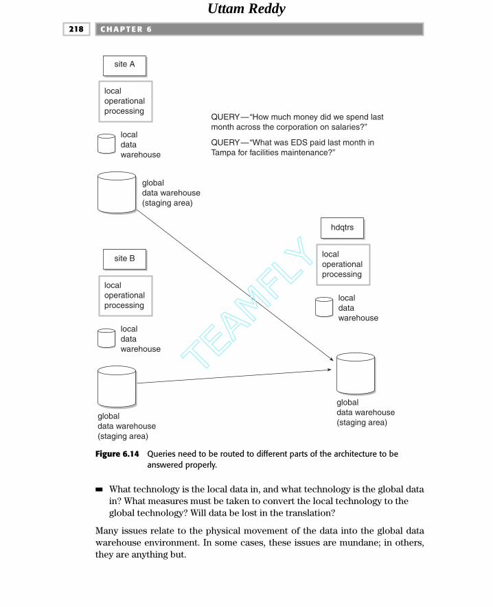
■■ What technology is the local data in, and what technology is the global datain? What measures must be taken to convert the local technology to theglobal technology? Will data be lost in the translation?

Many issues relate to the physical movement of the data into the global datawarehouse environment. In some cases, these issues are mundane; in others,they are anything but.

C H A P T E R 6218

QUERY—“How much money did we spend lastmonth across the corporation on salaries?”

QUERY—“What was EDS paid last month inTampa for facilities maintenance?”

site Asite A

localdatawarehouse



site Asite B

localdatawarehouse



site Ahdqtrs

localdatawarehouse



Figure 6.14 Queries need to be routed to different parts of the architecture to beanswered properly.

TEAMFLY

Team-Fly®

Uttam Reddy

A related yet separate issue not addressed in this chapter is global operationaldata. Thus far, this chapter has assumed that every local site has its own uniqueoperational data and processing. However, it is entirely possible that there is adegree of commonality between the operational systems found at each local site.In this case, some degree of corporate operational data and processing might bedesirable. For example, some customers may need to be handled globally, suchas large multinational corporations like Coca-Cola, McDonalds, IBM, and AT&T.Pricing considerations, size-of-order considerations, and delivery considerationsmay be treated differently globally than similar decisions are treated locally. Inthe case of global operational processing, that global operational data merelybecomes another source of data into the global data warehouse. But there is stillthe distinction between operational data and DSS informational data.

Underlying the whole issue of the distributed data warehouse is complexity. Ina simple central data warehouse environment, roles and responsibilities arefairly straightforward. In a distributed data warehouse environment, however,the issues of scope, coordination, meta data, responsibilities, transfer of data,local mapping, and more make the environment complex indeed.

One of the major considerations for a global data warehouse is whether thedata warehouse should be built centrally or globally. While tempting to say thata global data warehouse should be designed and built centrally, doing so ispatently a mistake. With a centralized construction of a global data warehouse,there is—at best—only a marginal local buy-in to the global data warehouse.This means that the definition of the mapping between the local systems andthe needs for global data is done centrally, not locally. To succeed, there mustbe local management and control of the mapping process. Stated differently,the single most difficult part of the building and population of the global datawarehouse is the mapping of the local data to the global data. And this mappingcannot be done centrally; it must be done locally.

For example, suppose the headquarters organization tries to map Brazilian datainto the global data warehouse. This poses the following problems:

■■ Portuguese is not the native tongue of the headquarters organization.

■■ Headquarters personnel do not understand local business practices andcustoms.

■■ Headquarters personnel do not understand local legacy applications.

■■ Headquarters personnel do not understand the local data warehouse.

■■ Headquarters personnel are not on hand to keep abreast of day-to-daychanges in local systems.

There are then a plethora of reasons why the mapping of local data into theglobal data warehouse environment cannot be done by centralized personnel.


Uttam Reddy

Therefore, the local organization must be a part of the building of the globaldata warehouse.

A final observation is that the local data needs to be in as flexible a form as pos-sible. This usually means that the local data must be organized relationally. Ifthe local data is organized in a star join multidimensional format, it will bedifficult to break apart and restructure for the global data warehouse.

The Technologically Distributed Data Warehouse

The spread of a company over multiple geographical locations or over manydifferent product lines is not the only reason why a distributed data warehouseis appealing. There are other rationales as well. One case for a different type ofa distributed warehouse is that of placing a data warehouse on the distributedtechnology of a vendor. Client/server technology fits this requirement nicely.

The first question is, can a data warehouse be placed on distributed technol-ogy? The answer is yes. The next question is, what are the advantages and dis-advantages of using distributed technology for a data warehouse? The firstadvantage of a technologically distributed data warehouse is that the entry costis cheap. In other words, the cost of hardware and software for a data ware-house when initially loaded onto distributed technology is much less than if thedata warehouse were initially loaded onto classical, large, centralized hard-ware. The second advantage is that there is no theoretical limit to how muchdata can be placed in the data warehouse. If the volume of data inside the ware-house begins to exceed the limit of a single distributed processor, then anotherprocessor can be added to the network, and the progression of adding data con-tinues in an unimpeded fashion. Whenever the data grows too large, anotherprocessor is added.

Figure 6.15 depicts a world in which there may be an infinite amount of data inthe data warehouse. This is appealing because a data warehouse will containmuch data (but not an infinite amount!).

There are, however, some considerations. As the data warehouse starts toexpand beyond a few processors (i.e., servers), an excessive amount of trafficstarts to appear on the network. The increased traffic appears when a requestfor data overlaps from one processor to another. For example, suppose oneprocessor holds data for the year 1998, another processor for 1999, another for2000, and yet another for 2001. When a request is made for data from 1998 to2001, the result set for that query must pass over the boundaries of the proces-sor that originally held the data. In this case, data from four processors mustbe gathered. In the process, data passes across the network and increases thetraffic.

C H A P T E R 6220

Uttam Reddy


A single server holds all thedata for the warehouse.

Now two servers hold thedata for the warehouse.

The number of servers that hold thewarehouse data can be expanded adinfinitum (at least in theory) for as muchdata as desired in the data warehouse.

day 1

day 2

day 3

Figure 6.15 The progression of adding more servers to hold the data warehouse data.

The issue arises not only of a query accessing data housed by multiple processors,but of a large amount of data needing to be transported from a single processor.For example, suppose a query wishes to access all 1999 data and all 2000 data.Such a query will pull data from one or the other processor. Figure 6.16 depicts aquery that wishes to access a large amount of data from multiple servers.

Techniques and approaches do of course exist to deal with a data warehousethat is technically distributed over multiple servers. Ironically, the problemsgrow with time, as the warehouse becomes fully populated and as the numberof servers grows. In the early days of a distributed data warehouse when thereis very little data and only a few servers, the problems discussed here are hardlyobvious. In the more mature days of a data warehouse, however, the data andthe processing environment become more difficult to manage.

The Independently EvolvingDistributed Data Warehouse

Yet a third flavor of distributed data warehouse is one in which independentdata warehouses are developed concurrently and in an uncontrolled manner.

The first step many corporations take in data warehousing is to put up a datawarehouse for a financial or marketing organization. Once success follows the

Uttam Reddy

initial warehouse effort, other parts of the corporation naturally want to build onthe successful first effort. In short order, the data warehouse architect has tomanage and coordinate multiple data warehouse efforts within the organization.

The Nature of the Development Efforts

The first issue facing the data architect who must manage multiple data ware-house development efforts is the nature of the development efforts. Unless thedata architect knows what kinds of efforts are occurring and how they relate tothe overall architecture, he or she will have a very difficult time managing andcoordinating them. Because the issues of development vary considerablydepending on the approach, different types of data warehouse developmentefforts require very different approaches to management.

Multiple data warehouse development efforts occur in four typical cases, asoutlined in Figure 6.17.

In the first, rare case shown in Figure 6.17, a corporation has totally separateand unintegrated lines of business for which data warehouses are being inde-pendently built by different development groups. The diverse lines of businessreport to the corporation, but other than sharing a company name, there is nobusiness integration or sharing of data within the company. Such a corporate

C H A P T E R 6222

datawarehouse

query

Figure 6.16 A query that accesses a large amount of data from multiple data ware-house servers.

Uttam Reddy

structure is not unknown, but it is not common. In this case, there is very littledanger that one data warehouse development effort will conflict with another.Accordingly, there is little or no need for cross-management and coordinationof data warehouse development efforts.


d/w Aline of business

A

d/w Bline of business

B

d/w Cline of business

C

d/w Dline of business

D

completely unintegrated lines of business each with their own data warehouses

northeastd/w

midwestd/w

westernd/w

southwestd/w

the same data warehouse but with distributed parts

lightlysummarized

OLAP

detaileddata

different levels of data within the same data warehouse

different non-distributed parts of the detailed level of the data warehouse

Figure 6.17 Four possible meanings to “multiple groups building the data warehouse,”each interpretation very different from the others.

Uttam Reddy

The second case of multiple data warehouse efforts occurring simultaneouslyhappens when a corporate distributed data warehouse is being built and variousdevelopment groups are creating different parts of the same data warehouse. Inthis case, the same detailed data is being built by different groups of developers,but the data is distributed across different locations. For example, suppose a carmanufacturer is building a manufacturing data warehouse in Detroit andanother manufacturing data warehouse in Canada. The same detailed data findsits way into the data warehouse in both places. Unless extraordinary measuresare taken, likely many conflicting analyses will occur. This case for multipledevelopment efforts is as common as the previous case is rare. Yet because thiscase is so common, it requires a great deal of attention. It requires discipline andclose coordination among the groups to achieve a collectively satisfying result.The danger of not coordinating this effort is that much waste may occur throughredundant storage and manipulation of massive amounts of data. If data is cre-ated redundantly, the resulting data warehouse may well be ineffective becausethere will be a classic spider web in the DSS environment.

The third case of multiple data warehouse development occurring simultane-ously happens when different groups are building different levels of data (i.e.,summarized data and detailed data) in the data warehouse environment. Likethe preceding case, this scenario is also very common. However, for a variety ofreasons, it is much easier to manage than either of the two previous cases.Because of the differences in the levels of data, there are different uses andexpectations. And coordination between the two groups is likely to be astraightforward exercise. For example, one group of people might be building adata warehouse to capture and analyze each bank transaction at the lowestlevel of detail. Another group of analysts might be creating customer recordssummarized up to the monthly level. The interface between the two groups issimple. The detailed transactions are summarized on a monthly basis to createthe aggregate/summary record for the customer.

The fourth case occurs when multiple groups are trying to build different partsof the current level of detail of the data warehouse environment in a nondis-tributed manner. This is a somewhat rare phenomenon, but when it occurs, itmandates special attention. There is much at stake in this last case, and the dataarchitect must be aware of what the issues are and how they relate to success.

Each of these cases are discussed in the following sections, along with theirissues, advantages, and disadvantages.

Completely Unrelated WarehousesThe building and operation of completely unrelated warehouses is shown inFigure 6.18. A corporation has four lines of business—golf course management,a steel mill, retail banking, and a fast-food franchise. There is no integration of

C H A P T E R 6224

Uttam Reddy

the businesses whatsoever. A customer of one business may be a customer ofanother business, and there is no desire to link the two relationships. The ongo-ing data warehouse efforts have no reason to be coordinated. All the way frommodeling to selection of base technology (i.e., platform, DBMS, access tools,development tools, etc.), each of the different businesses could operate as if itwere completely autonomous.

For all the autonomy of the lines of business, they are necessarily integrated atone level: the financial balance sheet. If the different lines of business report toa single financial entity, there must be integration at the balance-sheet level. Inthis situation, a corporate data warehouse might need to be built that reflectsthe corporate finances. Figure 6.19 shows a corporate financial data warehousesitting above the different businesses.

The financial corporate data warehouse contains simple (and abstract) entitiessuch as expenses, revenues, capital expenditures, depreciation, and the like.There is very little, if any, business data beyond that found on every balancesheet. (In other words, no attempt is made for a common corporate description


d/w Afast foodfranchise

d/w Bsteelmill

d/w Cretail

banking

d/w Dgolf course

management

Figure 6.18 Four totally independent enterprises where there is little or no integrationof data at the business level.


d/w Bsteelmill

d/w Cretail

banking

d/w Dgolf course

management

corporate financialdata model

Figure 6.19 Even the most disparate of business enterprises share common corporatefinancial data.

Uttam Reddy

of customer, product, sale, and so on in the financial data warehouse.) Ofcourse, the data feeding the corporate financial data warehouse depicted in Fig-ure 6.19 may come either from the “local” data warehouse or from the opera-tional systems found at the individual operating company level.

Meta data is vital at the local level. With a corporate financial data warehouse,it is also needed at the corporate financial level. However, in this case, becauseno real business integration exists, there is no need to tie any of the meta datatogether.

Distributed Data Warehouse Development

Unlike the case of the unrelated warehouses, most businesses have somedegree of integration among their disparate parts. Very few businesses are asautonomous as those depicted in Figure 6.19. A much more common scenariofor the development of multiple data warehouse efforts is shown in Figure 6.20.

In Figure 6.20 a corporation has different sites in different parts of the world—one in the United States and Canada, one in South America, one in the Far East,and one in Africa. Each site has its own unique data, with no overlap of data—particularly of detailed transaction data—from one site to the next. The com-pany wants to create a data warehouse for each of the disparate entities as afirst effort in achieving an architected environment. There is some degree ofbusiness integration among the different organizations. At the same time, it isassumed that distinct business practices are carried on in each locale. Such anorganization of corporate entities is common to many companies.

The first step many organizations make toward data warehousing is to create alocal data warehouse at each geographical entity. Figure 6.21 shows the cre-ation of a local data warehouse.

Each locale builds its own unique autonomous data warehouse according to itsneeds. Note that there is no redundant detailed data among the differentlocales, at least as far as transaction data is concerned. In other words, a unit of

C H A P T E R 6226

Africad/w

USd/w

Canadad/w

Far Eastd/w

South Americad/w

Figure 6.20 Logically the same data warehouse.

Uttam Reddy

data reflecting transactions that belongs in Africa would never be found in thelocal data warehouse for Europe.

There are several pros and cons to this approach to building the distributed cor-porate data warehouse. One advantage is that it is quick to accomplish. Eachlocal group has control over its design and resources. A sense of autonomy andcontrol may make each local organization happy. As such, the benefits of thedata warehouse can be proven throughout the corporation on a real-time basis.Within six months the local data warehouses can be up and running, and theorganization at the local level can be deriving the benefits. The disadvantage isthat if there is any commonality in the structure (not the content) of data acrossthe organization, this approach does nothing to recognize or rationalize thatcommonality.

Coordinating Development acrossDistributed Locations

An alternative approach is to try to coordinate the local data warehouse devel-opment efforts across the different local organizations. This sounds good in the-ory, but in execution it has not proved to be effective. The local developmentgroups never collectively move at the same pace, and the local groups look onthe central development group trying to coordinate the many local developmentefforts as a hindrance to progress. A separate data model is built to provide thefoundation of the data warehouse design for each of the separate locales.

One day, after the worth of data warehousing has been proven at the local level,the corporation decides to build a corporate data warehouse (see Figure 6.22).


Africad/w

USd/w

Canadad/w

Far Eastd/w

South Americad/w

Figure 6.21 Local data warehouses are built at each of the autonomous operating divi-sions.

Uttam Reddy

The corporate data warehouse will reflect the business integration across thedifferent divisions and locales. The corporate data warehouse will be related to,but still distinct from, the local data warehouses. The first step in building thecorporate data warehouse is to create a corporate data model for that portionof the business that will be reflected in the corporate data warehouse. As a gen-eral rule, the corporate data model that is built for the first iteration of the cor-porate data warehouse will be small and simple, and it will be limited to asubset of the business. Figure 6.23 illustrates the building of the corporate datamodel after which the corporate data warehouse will be shaped.

The Corporate Data Model—Distributed

The corporate data model reflects the integration of business at the corporatelevel. As such, the corporate data model may overlap considerably with por-tions of the local data models. Such an overlap is healthy and normal. In othercases, the corporate data model will be different from the local data models. Inany case, it is up to the local organization to determine how the fit is to be madebetween the corporate need for data and the local ability to provide it. The localorganization knows its own data better than anyone, and it is best equipped toshow how local data needs to be shaped and reshaped to meet the specifica-tions of the corporate design of data for the data warehouse.

C H A P T E R 6228

Africad/w

USd/w

Canadad/w

Far Eastd/w

South Americad/w

corporatedata warehouse

Figure 6.22 One day the decision is made to build a corporate data warehouse.

TEAMFLY

Team-Fly®

Uttam Reddy

While there may very well be overlap in the structural design of data from onelocal level to the next, there is no overlap to any great extent in the content ofdata. Figure 6.24 shows the building and population of the corporate data ware-house from the local levels.

The source of the data going to the corporate data warehouse can come fromthe local data warehouse or from the local operational systems. The determi-nation of the system of record should be a decision that is made entirely at thelocal level. Most certainly, several iterations of definition of the system ofrecord will be needed.

In addition, an important design issue is how to create and transport the localsystem of record data from the technology found at the local level into the tech-nology of the corporate data warehouse. In some cases, the official “staged”data is kept at the local level. In other cases, the staged data is passed on to thecorporate environment with no access at the local level.

As a rule, the data in the corporate data warehouse is simple in structure andconcept. Figure 6.25 shows that data in the corporate data warehouse appearsto be detailed data to the DSS analyst at the corporate level, and at the sametime it appears to be summary data to the DSS analyst at the local level. Thisapparent contradiction is reconciled by the fact that the appearance of summa-rization or detail is strictly in the eye of the beholder.


Africad/w

USd/w

Canadad/w

Far Eastd/w

South Americad/wcorporate

data warehouse

corporatedata model

Figure 6.23 The corporate data model is created.

Uttam Reddy

C H A P T E R 6230

Africad/w

USd/w

Canadad/w

Far Eastd/w

South Americad/w

corporatedata warehouse

Figure 6.24 The corporate data warehouse is loaded from the different autonomousoperating companies.

SouthAmerica

d/w

corporatedata

warehouse

summarydata

detaileddata

Figure 6.25 What is summary at one level is detailed at another.

Uttam Reddy

The corporate data warehouse of the distributed database can be contrastedwith the corporate financial data warehouse of the completely unrelated com-panies. Figure 6.26 makes this comparison.

In many ways, the data warehouse of the distributed corporation is very similarto the data warehouse of the unrelated companies. However, although there aresimilarities in design and operation, there is one major difference. The corpo-rate distributed data warehouse extends into the business itself, reflecting theintegration of customer, vendor, product, and so forth. As such, the corporate



d/w Bsteelmill

d/w Cretail

banking

d/w Dgolf course

management

corporate financialdata model

Africad/w

USd/w

Canadad/w

Far Eastd/w

SouthAmerica

d/w

corporatedata

warehousestrong similarities

Figure 6.26 The data warehouse of a distributed corporation can be very similar to thatof unrelated companies.

Uttam Reddy

distributed data warehouse represents the very fabric of the business itself.The corporate data warehouse for unrelated companies, though, is for financealone. The instant that there is a desire to use the corporate financial datawarehouse for anything other than the financial relationship of the differentparts of the corporation, there will be disappointment with the corporatefinancial data warehouse. The difference between the two data warehouses,then, is one of depth.

Meta Data in the Distributed Warehouse

Meta data plays a very important role across the distributed corporate datawarehouse. It is through meta data that the coordination of the structure ofdata is achieved across the many different locations where the data warehouseis found. Not surprisingly, meta data provides the vehicle for the achievementof uniformity and consistency.

Building the Warehouse on Multiple Levels

The third scenario of a company’s simultaneous data warehouse developmentoccurs when different development groups are building different levels of thedata warehouse, as seen in Figure 6.27. This case is very different from the caseof the distributed data warehouse development. In this case, Group A is build-ing the high level of summarization of data, Group B is building the middle levelof summarization, and Group C is building the current level of detail.

The scenario of multiple levels of data warehouse development is very com-mon. Fortunately, it is the easiest scenario to manage, with the fewest risks.

C H A P T E R 6232

detailed data

lightlysummarized

OLAP

developmentgroup A

developmentgroup B

developmentgroup C

Figure 6.27 Different development groups are developing different parts of the datawarehouse environment at different levels of the architecture.

Uttam Reddy

The primary concern of the data architect is to coordinate the efforts of thedifferent development teams, both in terms of the specification of content andstructure and in terms of the timing of development. For example, if Group A is significantly ahead of Group B or C, there will be a problem: When Group A is ready to populate its databases at the summary level, there may be nodetailed data to work with.

One of the interesting aspects of different groups building different levels ofsummarization of the same data warehouse is that it is the group that is build-ing the current level of detail that uses the data warehouse data model. Fig-ure 6.28 illustrates this relationship.

The data model for the data warehouse directly reflects the design and devel-opment effort by the group doing current-level detailed analysis and design. Ofcourse, indirectly the data warehouse data model reflects the needs of allgroups. But because other groups are summarizing from the data found at thecurrent level of detail, they have their own interpretation of what is needed. Inmost cases, the groups working on the higher levels of summarization havetheir own data models that reflect their own specialized needs.

One of the issues of managing multiple groups building different levels of sum-marization is the technological platforms on which the data warehouse levelsare built. Normally, different groups choose different technological platforms.In fact, for the different development groups to choose the same platformwould be very unusual. There are several reasons for this, though the primaryone is cost. The detailed level of data requires an industrial-strength platformbecause of the large volume of data that will have to be handled. The different


detailed data

lightlysummarized

OLAP

developmentgroup A

developmentgroup B

developmentgroup C

data model

Figure 6.28 The development organization that is developing the lowest level of detailis the organization that uses the data model.

Uttam Reddy

levels of summarization will require much less data, especially at the higher lev-els of summarization. It is overkill (and expensive) to place the higher levels ofsummarized data on the same platform as the detailed data (although it can bedone).

Another reason is that the alternative platforms offer a wide variety of special-ized software, much of which is not to be found on the monolithic platformsthat house detailed data. In any case, whether the different levels of data are ona single platform or on multiple platforms, meta data must be carefully storedand managed, so that continuity from one level of detail to the next can bemaintained.

Because different platforms are commonly used for the different levels of datathat are being developed by different groups, the issue of interconnectivityarises. Figure 6.29 shows the need for interconnectivity from one level to thenext.

Several aspects of interconnectivity need to be addressed. One issue is the com-patibility of access at the call level. In other words, is there compatible syntaxbetween the two technologies that make up the detailed and the summary databetween any two levels of the warehouse? If there is not at least some degree ofcompatibility, the interface will not be usable. Another aspect of the intercon-nectivity issue is the effective bandwidth of the interface. If very heavy traffic isbeing created by processing that occurs on either level of the data warehouse,the interface between the two environments can become a bottleneck.

However the groups that work on the data warehouse are coordinated, onerequirement remains clear: The group that manages the lower-level detail mustform a proper foundation of data for those groups that will be summarizing thedata and creating a new level. This need is depicted in Figure 6.30.

The coordination among the groups can be as simple as an agreement on a datamodel that satisfies the needs of all parties. Or the agreement can be muchmore elaborate, if circumstances warrant.

C H A P T E R 6234

detailed data

lightlysummarized

OLAP

Figure 6.29 Interconnectivity between the different levels of the data warehouse is animportant issue.

Uttam Reddy

The coordination of the development efforts is another matter. There must be atime-sequenced arrangement among the different development groups so thatno one group arrives at a point of needing data that has not yet been gatheredat a lower level.

Multiple Groups Building the Current Level of Detail

An infrequent set of circumstances occurs when multiple development groupsattempt to build the current level of detail in a data warehouse in a nondistrib-uted manner. Figure 6.31 illustrates this phenomenon.

As long as the groups that are developing the current level of detail are devel-oping mutually exclusive sets of data, there is little difficulty. In this case, if thedevelopment groups are working from a common data model and the differentgroups’ platforms are compatible, no problems should ensue. Unfortunately,mutually exclusive data sets are the exception rather than the rule. It is muchmore common for the multiple development groups to be designing and popu-lating some or all of the same data.

A series of problems arise when the groups overlap. The first problem is cost—in particular, the cost of storage and processing. The volumes of data that arefound at the current detailed level are such that any amount of redundancymust be questioned, much less wholesale redundancy. The cost of processingthe detail is likewise a major issue.

The second, more insidious issue is the introduction of the spider web into theDSS environment. With massive amounts of redundant detailed data, it isalmost axiomatic that misinterpretation of data caused by redundancy willoccur, where there is no effective reconcilability. Creating large amounts of


lightlysummarized

detailed data

detail

summary

Figure 6.30 The detailed level forms the foundation for the summary level of data.

Uttam Reddy

redundant detailed data is a very undesirable condition for the detailed level ofdata in the data warehouse and defeats its purpose. If multiple developmentgroups will be doing concurrent design and population in the current level ofdetail, great care must be taken to ensure that no redundant detailed data iscreated.

To ensure that no redundant data is developed, it is necessary to create a datamodel that reflects the common detailed data. Figure 6.32 shows that multipledevelopment groups have combined their interests to create a common datamodel. In addition to the currently active development groups, other groupsthat will have future requirements but who are not currently in a developmentmode may also contribute their requirements. (Of course, if a group knows itwill have future requirements but is unable to articulate them, then thoserequirements cannot be factored into the common detailed data model.) Thecommon detailed data model reflects the collective need among the differentgroups for detailed data in the data warehouse.

The data model forms the basis of the design for the data warehouse. Fig-ure 6.33 shows that the data model will be broken up into many tables as designprogresses, each of which physically becomes part of the warehouse.

Because the data model is broken into multiple physical tables at the momentof implementation, the development process for the data warehouse can pro-ceed in an iterative manner. There is no need to build all of the tables at once.In fact, a good reason to build only a few tables at a time is so that the end user

C H A P T E R 6236

developmentgroup A

developmentgroup B

developmentgroup C

developmentgroup D

developmentgroup E

Figure 6.31 Different development groups that are developing the current level ofdetail for the data warehouse.

Uttam Reddy


data unique todevelopment

group A


group B


group C


group D

commondata model

data common todevelopment

groups A, B, C, D

Figure 6.32 A data model identifies data that is common to all the developmentgroups.

customermovement

historysales

history

vendorhistory

partshistory

customersurveyhistory

substitutepart

history

customerhistory

salespricinghistory

shipmenthistory

customercomplaint

history

partsrejecthistory

shipmentarrivalhistory

shipmentbreakage

history

commondata model

Figure 6.33 The data warehouse is physically manifested over multiple physical tablesand databases.

Uttam Reddy

feedback can be factored into the modification of the table, if necessary, with aminimum of fuss. In addition, because the common data model is broken intomultiple tables, adding new tables at a later time to reflect requirements thatare now unknown is not a problem.

Different Requirements at Different Levels

Normally different groups have unique requirements (see Figure 6.34). Theserequirements result in what can be termed “local” current-level detail. The localdata is certainly part of the data warehouse. It is, however, distinctively differ-ent from the “common” part. The local data has its own data model, usuallymuch smaller and simpler than the common detailed data model.

There is, of necessity, nonredundancy of data across all of the detailed data.Figure 6.35 makes this point clear.

Of course, the nonredundancy of the data is restricted to nonkey data. Redun-dancy exists at the key level because a form of foreign key relationships is usedto relate the different types of data. Figure 6.36 shows the use of foreign keys.

The foreign keys found in the tables shown in Figure 6.36 are quite differentfrom the classical foreign key relationships that are governed by referentialintegrity. Because the data in the data warehouse is gathered by and stored in

C H A P T E R 6238


group A


group B


group Cdata unique todevelopment

group D

commondata model


groups A, B, C, D

local currentlevel detail

Figure 6.34 Just because data is not common to all development groups does notmean that it does not belong in the current-level detail of the data ware-house.

TEAMFLY

Team-Fly®

Uttam Reddy

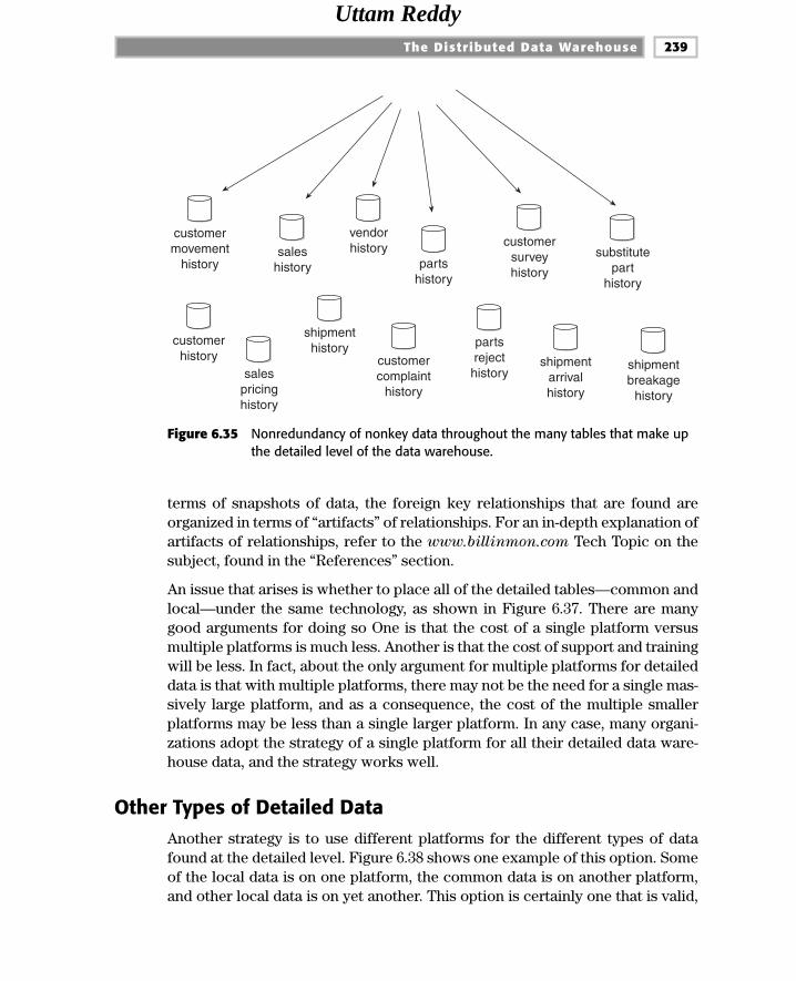
terms of snapshots of data, the foreign key relationships that are found areorganized in terms of “artifacts” of relationships. For an in-depth explanation ofartifacts of relationships, refer to the www.billinmon.com Tech Topic on thesubject, found in the “References” section.

An issue that arises is whether to place all of the detailed tables—common andlocal—under the same technology, as shown in Figure 6.37. There are manygood arguments for doing so One is that the cost of a single platform versusmultiple platforms is much less. Another is that the cost of support and trainingwill be less. In fact, about the only argument for multiple platforms for detaileddata is that with multiple platforms, there may not be the need for a single mas-sively large platform, and as a consequence, the cost of the multiple smallerplatforms may be less than a single larger platform. In any case, many organi-zations adopt the strategy of a single platform for all their detailed data ware-house data, and the strategy works well.

Other Types of Detailed DataAnother strategy is to use different platforms for the different types of datafound at the detailed level. Figure 6.38 shows one example of this option. Someof the local data is on one platform, the common data is on another platform,and other local data is on yet another. This option is certainly one that is valid,


customermovement

historysales

history

vendorhistory

partshistory

customersurveyhistory

substitutepart

history

customerhistory

salespricinghistory

shipmenthistory

customercomplaint

history

partsrejecthistory

shipmentarrivalhistory

shipmentbreakage

history

Figure 6.35 Nonredundancy of nonkey data throughout the many tables that make upthe detailed level of the data warehouse.

Uttam Reddy

and it often satisfies the different political needs of the organization. With thisoption each group doing development can feel that it has some degree of con-trol of at least its own peculiar needs. Unfortunately, this option has severalmajor drawbacks. First, multiple technologies must be purchased and sup-ported. Second, the end user needs to be trained in different technologies. Andfinally, the boundaries between the technologies may not be as easy to cross.Figure 6.39 illustrates this dilemma.

C H A P T E R 6240

key

..........

..........

..........

..........

foreign key

foreign key

vendorhistory

key

..........

..........

..........

..........

foreign key

shipmenthistory

key

..........

..........

..........

..........

foreign key

foreign key

saleshistory

key

..........

..........

..........

..........

foreign key

foreign key

partshistory

key

..........

..........

..........

..........

foreign key

customerhistory

Figure 6.36 Foreign keys in the data warehouse environment.

Uttam Reddy



group A


group B


group C data unique todevelopment

group D


groups A, B, C, D

common technological platform

Figure 6.37 The different types of data in the detailed level of the data warehouse allon a common platform.


group A


group B



group D


groups A, B, C, D

platform A

platform B

platform C

Figure 6.38 In this case, the different parts of the detailed level of the data warehouseare scattered across different technological platforms.

Uttam Reddy

If there are to be multiple technologies supporting the different levels of detailin the data warehouse, it will be necessary to cross the boundaries between thetechnologies frequently. Software that is designed to access data across differ-ent technological platforms is available. Some of the problems that remain areshown in Figure 6.40.

One problem is in the passage of data. If multi-interfaced technology is used forthe passage of small amounts of data, then there is no problem with perfor-mance. But if multi-interfaced technology is used to pass large amounts of data,then the software can become a performance bottleneck. Unfortunately, in aDSS environment it is almost impossible to know how much data will beaccessed by any one request. Some requests access very little data; otherrequests access large amounts of data. This problem of resource utilization andmanagement manifests itself when detailed data resides on multiple platforms.

C H A P T E R 6242


group A


group B



group D


groups A, B, C, D

platform A

platform B

platform C

data transfer

Figure 6.39 Data transfer and multiple table queries present special technological problems.

Uttam Reddy

Another related problem is “leaving” detailed data on one side of the data ware-house after it has been transported from the other side. This casual redeploy-ment of detailed data has the effect of creating redundancy of data at thedetailed level, something that is not acceptable.


platform B

platform A

platform C

bulk transfer of data

leaving data after analysis is complete

Figure 6.40 Some problems with interfacing different platforms.

customercomplaint

history

shipmenthistory

customermovement

historysales

history

vendorhistory

partshistory

customerhistory sales pricing

history

meta data

Figure 6.41 Meta data sits on top of the actual data contents of the data warehouse.

Uttam Reddy

Meta Data

In any case, whether detailed data is managed on a single technology or on mul-tiple technologies, the role of meta data is not diminished. Figure 6.41 showsthat meta data is needed to sit on top of the detailed data warehouse data.

Multiple Platforms for Common Detail Data

One other possibility worth mentioning is using multiple platforms for commondetail of data. Figure 6.42 outlines this scenario.

While such a possibility is certainly an option, however, it is almost never agood choice. Managing common current detailed data is difficult enough. Thevolumes of data found at that level present their own unique problems for man-agement. Adding the complication of having to cross multiple technologicalplatforms merely makes life more difficult. Unless there are very unusual miti-gating circumstances, this option is not recommended.

The only advantage of multiple platforms for the management of commondetail is that this option satisfies immediate political and organizational differ-ences of opinion.

C H A P T E R 6244

platform A platform B platform C

common data across manydevelopment groups

current detailed data

Figure 6.42 Common detailed data across multiple platforms-a real red flag in all cases.

Uttam Reddy

Summary

Most environments operate from a single centralized data warehouse. But insome circumstances there can be a distributed data warehouse. The three typesof distributed data warehouses are as follows:

■■ Data warehouses serving global businesses where there are local opera-tions and a central operation

■■ Technologically distributed data warehouses where the volume of data issuch that the data is spread over multiple physical volumes

■■ Disparate data warehouses that have grown separately through lack oforganizational or political alignment

Each type of distributed data warehouses has its own considerations.

The most difficult aspect of a global data warehouse is the mapping done at thelocal level. The mapping must account for conversion, integration, and differ-ent business practices. The mapping is done iteratively. In many cases, theglobal data warehouse will be quite simple because only the corporate data thatparticipates in business integration will be found in the global data warehouse.Much of the local data will never be passed to or participate in the loading ofthe global data warehouse. Access of global data is done according to the busi-ness needs of the analyst. As long as the analyst is focusing on a local businesspractice, access to global data is an acceptable practice.

The local data warehouses often are housed on different technologies. In addi-tion, the global data warehouse may be on a different technology than any ofthe local data warehouses. The corporate data model acts as the glue that holdsthe different local data warehouses together, as far as their intersection at theglobal data warehouse is concerned. There may be local data warehouses thathouse data unique to and of interest to the local operating site. There may alsobe a globally distributed data warehouse. The structure and content of the dis-tributed global data warehouse are determined centrally, whereas the mappingof data into the global data warehouse is determined locally.

The coordination and administration of the distributed data warehouse envi-ronment is much more complex than that of the single-site data warehouse.Many issues relate to the transport of the data from the local environment tothe global environment, including the following questions:

■■ What network technology will be used?

■■ Is the transport of data legal?

■■ Is there a processing window large enough at the global site?

■■ What technological conversion must be done?


Uttam Reddy

Uttam Reddy

Executive Information Systems and the Data Warehouse

C H A P T E R 7

Prior to data warehousing, there were executive information systems (EIS). EISwas a notion that computation should be available to everyone, not just theclerical community doing day-to-day transactions. EIS presented the executivewith a set of appealing screens. The idea was that the elegance of the screenpresentation would beguile the executive. While there certainly is merit to theidea that the world of computation should be open to the executive, thefounders of EIS had no concept of the infrastructure needed to get those num-bers to the executive. The entire idea behind EIS was presentation of informa-tion with no real understanding of the infrastructure needed to create thatinformation in the first place. When the data warehouse first appeared, the EIScommunity roundly derided it as a complex discipline that required getting thehands dirty. EIS was a high-minded, elegant discipline that was above the hardwork and management of complexity involved in a data warehouse. The EIScommunity decided that executives had better things to do than worry aboutsuch issues as sources of data, quality of data, currency of data, and so forth.And so EIS died for lack of an infrastructure. It hardly mattered that the pre-sentation to the executive was elegant if the numbers being presented wereunbelievable, inaccurate, or just plain unavailable.

This chapter first appeared just as EIS was on its way out. As originally written,this chapter was an attempt to appeal to the EIS community, based on the ratio-nality of the necessity of an infrastructure. But the wisdom of the EIS com-munity and its venture capital backers was such that there was to be no

247

Uttam Reddy

relationship between data warehousing and EIS. When it came to the infra-structure needed to support the grandiose plans of the EIS community, the EIScommunity and the venture capital community just didn’t get it.

EIS as it was known in its earliest manifestation has all but disappeared. But thepromises made by EIS are still valuable and real. Consequently EIS has reap-peared in many forms today—such as OLAP processing and DSS applicationssuch as customer relationship management (CRM)—and those more modernforms of EIS are very much related to data warehousing, unlike the earliestforms of EIS.

EIS—The Promise

EIS is one of the most potent forms of computing. Through EIS, the executiveanalyst can pinpoint problems and detect trends that are of vital importance tomanagement. In a sense, EIS represents one of the most sophisticated applica-tions of computer technology.

EIS processing is designed to help the executive make decisions. In manyregards, EIS becomes the executive’s window into the corporation. EIS pro-cessing looks across broad vistas and picks out the aspects that are relevant tothe running of the business. Some of the typical uses of EIS are these:

■■ Trend analysis and detection

■■ Key ratio indicator measurement and tracking

■■ Drill-down analysis

■■ Problem monitoring

■■ Competitive analysis

■■ Key performance indicator monitoring

A Simple Example

As an example of how EIS analysis might appear to an executive, consider Fig-ure 7.1, which shows information on policies offered by an insurance company.Quarter by quarter, the new life, health, and casualty policy sales are tracked.The simple graph shown in Figure 7.1 is a good starting point for an executive’sprobing into the state of the business. Once the executive has seen the overallinformation, he or she can probe more deeply, as shown by the trend analysis inFigure 7.2.

In Figure 7.2, the executive has isolated new casualty sales from new life salesand new health sales. Looking just at new casualty sales, the executive identi-

C H A P T E R 7248

TEAMFLY

Team-Fly®

Uttam Reddy

fies a trend: New casualty sales are dropping off each quarter. Having identifiedthe trend, the executive can investigate why sales are dropping.

Executive Information Systems and the Data Warehouse 249

1stqtr

2ndqtr

3rdqtr

4thqtr

1stqtr

2ndqtr

500

400

300

200

100

executives and EIS

totalpolicies

new life policiesnew health policiesnew casualty policies

Figure 7.1 A chart typical of EIS processing.

1stqtr

2ndqtr

3rdqtr

4thqtr

1stqtr

2ndqtr

400

300

200

100

new casualty policies

what do executives see in EIS.

Figure 7.2 Trends—new casualty policy sales are dropping off.

Uttam Reddy

The EIS analysis alerts the executive as to what the trends are. It is then up tohim or her to discover the underlying reasons for the trends.

The executive is interested in both negative and positive trends. If business isgetting worse, why, and at what rate? What can be done to remedy the situa-tion? Or, if business is picking up, who and what are responsible for the upturn?What can be done to accelerate and accentuate the success factors? Can thesuccess factors be applied to other parts of the business?

Trends are not the only type of analysis accommodated by EIS. Another type ofuseful analysis is comparisons. Figure 7.3 shows a comparison that might befound in an EIS analysis.

Looking at fourth-quarter data, first-quarter data, and second-quarter data inFigure 7.3, the question can be asked, “Why is there such a difference in sales ofnew health policies for the past three quarters?” The EIS processing alerts themanager to these differences. It is then the job of the EIS analyst to determinethe underlying reasons.

For the manager of a large, diverse enterprise, EIS allows a look at the activitiesof the enterprise in many ways. Trying to keep track of a large number of activ-

C H A P T E R 7250

1stqtr

2ndqtr

3rdqtr

4thqtr

1stqtr

2ndqtr

500

400

300

200

100

new life policiesnew health policiesnew casualty policies

comparisons

Figure 7.3 Why is there an extreme difference in sales of new health policies for thepast three quarters?

Uttam Reddy

ities is much more difficult than trying to keep track of just a few activities. Inthat sense, EIS can be used to expand the scope of control of a manager.

But trend analysis and comparisons are not the only ways that the manager canuse EIS effectively. Another approach is to “slice-and-dice.” Here the analysttakes basic information, groups it one way, and analyzes it, then groups itanother way and reanalyzes it. Slicing and dicing allows the manager to havemany different perspectives of the activities that are occurring.

Drill-Down Analysis

To do slicing and dicing, it is necessary to be able to “drill down” on data.Drilling down refers to the ability to start at a summary number and to breakthat summary into a successively finer set of summarizations. By being able toget at the detail beneath a summary number, the manager can get a feel for whatis happening, especially where the summary number is surprising. Figure 7.4shows a simple example of drill-down analysis.

In Figure 7.4, the manager has seen second-quarter summary results and wantsto explore them further. The manager then looks at the regions that have con-tributed to the summary analysis. The figures analyzed are those of the Westernregion, the Southeast region, the Northeast region, and the Central region. Inlooking at the numbers of each region, the manager decides to look moreclosely at the Northeast region’s numbers.


Western region

Southeast region

Northeast region

Central region

New York City

Albany

Schenectady

Long Island

Ithaca

White Plains

Poughkeepsie

Other

New York

Massachusetts

Connecticut

Pennsylvania

New Jersey

Virginia

Maine, RI, Vermont

2ndqtr

Figure 7.4 To make sense of the numbers shown by EIS, the numbers need to supporta drill-down process.

Uttam Reddy

The Northeast’s numbers are made up of totals from New York, Massachusetts,Connecticut, Pennsylvania, New Jersey, Virginia, Maine, Rhode Island, and Ver-mont. Of these states, the manager then decides to look more closely at thenumbers for New York state. The different cities in New York state that haveoutlets are then queried.

In each case, the manager has selected a path of going from summary to detail,then to a successively lower level. In such a fashion, he or she can determinewhere the troublesome results are. Once having identified the anomalies, themanager then knows where to look more closely.

Yet another important aspect of EIS is the ability to track key performance indi-cators. Although each corporation has its own set, typical key performanceindicators might be the following:

■■ Cash on hand

■■ Customer pipeline

■■ Length of sales cycle

■■ Collection time

■■ New product channel

■■ Competitive products

Each corporation has several key performance indicators that—in a single mea-surement—tell an important story about some aspect of the life of the corpora-tion. On their own, the key performance indicators say a lot about what is goingon in the corporation. Taken over time, the key performance indicators sayeven more because they indicate trends.

It is one thing to say that cash on hand is $X. It is even more powerful to say thattwo months ago cash on hand was $Z, one month ago cash on hand was $Y, andthis month cash on hand is $X. Looking at key performance indicators overtime is one of the most important things an executive can do, and EIS is idealfor this purpose.

There is plenty of very sophisticated software that can be used in EIS to presentthe results to a manager. The difficult part of EIS is not in the graphical presen-tation but in discovering and preparing the numbers that go into the graphics,as seen in Figure 7.5.

EIS is perfectly capable of supporting the drill-down process from the graphicalperspective as long as the data exists in the first place. However, if the data toanalyze does not exist, the drill-down process becomes very tedious and awk-ward, certainly not something the executive wants to do.

C H A P T E R 7252

Uttam Reddy

Supporting the Drill-Down Process

Creating the basis of data on which to perform drill-down analysis, then, is themajor obstacle to successfully implementing the drill-down process, as seen inFigure 7.6. Indeed, some studies indicate that $9 is spent on drill-down datapreparation for every $1 spent on EIS software and hardware.

Exacerbating the problem is the fact that the executive is constantly changinghis or her mind about what is of interest, as shown in Figure 7.7. On day 1, theexecutive is interested in the corporation’s financial activities. The EIS analystmakes a big effort to develop the underlying data to support EIS interest. Thenon day 2, there is an unexpected production problem, and management’s atten-tion turns there. The EIS analyst scurries around and tries to gather the dataneeded by the executive. On day 3, the EIS analyst is directed to the problemsthat have developed in shipping. Each day there is a new focus for the execu-tive. The EIS analyst simply cannot keep up with the rate at which the execu-tive changes his or her mind.

Management’s focus in the running of the business shifts with every new prob-lem or opportunity that arises. There simply is no predictable pattern for whatmanagement will be interested in tomorrow. In turn, the EIS analyst is at theend of a whip—the wrong end! The EIS analyst is forever in a reactive state.Furthermore, given the work that is required of the EIS analyst to build the baseof data needed for EIS analysis, the EIS analyst is constantly swamped.


EIS software and thedrill-down process

Figure 7.5 EIS software supports the drill-down process as long as the data that isneeded is available and is structured properly.

Uttam Reddy

The problem is that there is no basis of data from which the EIS analyst can eas-ily work. Each new focus of management requires an entirely different set of datafor the EIS analyst. There is no infrastructure to support the EIS environment.

The Data Warehouse as a Basis for EIS

It is in the EIS environment that the data warehouse operates in its most effec-tive state. The data warehouse is tailor-made for the needs of the EIS analyst.Once the data warehouse has been built, the job of the EIS is infinitely easierthan when there is no foundation of data on which the EIS analyst can operate.Figure 7.8 shows how the data warehouse supports the need for EIS data.

With a data warehouse, the EIS analyst does not have to worry about the fol-lowing:

■■ Searching for the definitive source of data

■■ Creating special extract programs from existing systems

■■ Dealing with unintegrated data

■■ Compiling and linking detailed and summary data and the linkage betweenthe two

■■ Finding an appropriate time basis of data (i.e., does not have to worryabout finding historical data)

■■ Management constantly changing its mind about what needs to be lookedat next

In addition, the EIS analyst has a rich supply of summary data available.

C H A P T E R 7254

Buying and installingthe EIS software is fast

and easy.

Figure 7.6 Creating the base of data on which to do EIS is the hard part.

Uttam Reddy


mgmt

mgmt

mgmt

Management is interested in financial activities.

day 1

day 2

There is aproductionproblem.

financial

day 3production

financialSuddenly there is ashipment problem.

Figure 7.7 The constantly changing interests of executives.

Uttam Reddy

In short, the data warehouse provides the basis of data-the infrastructure—thatthe EIS analyst needs to support EIS processing effectively. With a fully popu-lated data warehouse in place, the EIS analyst can be in a proactive stance—notan eternally reactive stance—with regard to answering management’s needs.The EIS analyst’s job changes from that of playing data engineer to that of doingtrue analysis, thanks to the data warehouse.

Yet another very important reason why the data warehouse serves the needs ofthe world of EIS is this: The data warehouse operates at a low level of granu-larity. The data warehouse contains—for lack of a better word—atomic data.The atomic data can be shaped one way, then another. When management hasa new set of needs for information that has never before been encountered inthe corporation, the very detailed data found in the data warehouse sits, wait-ing to be shaped in a manner suited to management’s needs. Because of thegranular atomic data that resides in the data warehouse, analysis is flexible andresponsive. The detailed data in the data warehouse sits and waits for futureunknown needs for information. This is why the data warehouse turns an orga-nization from a reactive stance to a proactive stance.

Where to Turn

The EIS analyst can turn to various places in the architecture to get data. In Fig-ure 7.9, the EIS analyst can go to the individual level of processing, the depart-

C H A P T E R 7256

mgmt

the unpredictable natureof management’s focus

data warehouse

Figure 7.8 The data warehouse supports management’s need for EIS data.

Uttam Reddy

mental (data mart) level of processing, the lightly summarized level of process-ing, or the archival/dormant level of data. In addition, there is a normalsequence or hierarchy in which the EIS analyst goes after data to serve man-agement’s needs (see Figure 7.9).

There is a very good reason for the order shown, as indicated in Figure 7.10. Bygoing from the individual level of processing to the archival/dormant level, theanalyst does de facto drill-down analysis. The most summarized data found inthe architected environment is at the individual level. The supporting level ofsummary for the individual level is the departmental (data mart) level. Sup-porting the summaries at the departmental (data mart) level is data at the datawarehouse lightly summarized level. Finally, the light summarization at the datawarehouse level is supported by archival/dormant data. The sequence of sum-maries just described is precisely what is required to support drill-down EISanalysis.

Almost by default, the data warehouse lays a path for drill-down analysis. At thedifferent levels of the data warehouse, and throughout the summarization


individualoper datawarehouse

dept(data mart)

1

lightlysummarized

3

4

truearchival

2

departmental

EIS

Figure 7.9 Where EIS goes to retrieve data.

Uttam Reddy

process, data is related by means of a key structure. The key structure itself, orthe derivations of the key structure, allow the data to be related so that drill-down analysis is easy and natural.

The ways that EIS is supported by the data warehouse are illustrated in Fig-ure 7.11.

The EIS function uses the following:

■■ The data warehouse for a readily available supply of summary data

■■ The structure of the data warehouse to support the drill-down process

■■ Data warehouse meta data for the DSS analyst to plan how the EIS systemis built

■■ The historical content of the data warehouse to support the trend analysisthat management wishes to see

■■ The integrated data found throughout the data warehouse to look at dataacross the corporation

Event Mapping

A useful technique in using the data warehouse for EIS processing is event map-ping. The simplest way to depict event mapping is to start with a simple trend line.

C H A P T E R 7258

1

lightlysummarized

3

4

truearchival

detaileddata

2

departmental

EIS

verysummarizeddata

repetitivesummarydata

Figure 7.10 In going from individual levels of processing to true archival data, the drill-down process is accommodated.

TEAMFLY

Team-Fly®

Uttam Reddy

Figure 7.12 shows that corporate revenues have varied by month, as expected.The trend has been calculated from data found in the data warehouse. Thetrend of revenues in and of itself is interesting but gives only a superficial viewof what is going on with the corporation. To enhance the view, events aremapped onto the trend line.

In Figure 7.13, three notable events have been mapped to the corporate revenuetrend line—the introduction of a “spring colors” line of products, the advent ofa sales incentive program, and the introduction of competition. Now the rela-tionship between corporate revenue and significant events begins to take on adifferent perspective. Looking at the diagram in Figure 7.13, one might draw theconclusion that the introduction of a new line of products and a new incentiveplan have boosted revenue and that competition is starting to have an effect inthe latter part of the year.

For some sorts of events, event mapping is the only way to measure the results.Some events and activities cannot be measured directly and have to be


metadata

1

2

3

4 5

drilldown

drilldown

historyintegration

EIS

drilldown

Figure 7.11 How EIS is supported by the data warehouse.

Uttam Reddy

measured in a correlative fashion. Cost justification and actual cost benefit can-not be measured any other way for some types of events.

Misleading conclusions can be drawn, though, by looking at correlative infor-mation. It often helps to look at more than one set of trends that relate to theevents at hand. As an example, Figure 7.14 shows that corporate revenues arematched against the consumer confidence index to produce a diagram packedwith even more perspective. Looking at the figure shown, the executive canmake up his or her own mind whether events that have been mapped haveshaped sales.

C H A P T E R 7260

corporate revenues

Jan Feb Mar Apr May Jun Jul Aug Sep Oct Nov

Figure 7.12 Simple trends.

corporate revenues


introduction of“spring colors”

options salesmen’snew incentive

plan

competition’s nextyear’s linepromotion

Figure 7.13 Mapping events against a trend line.

Uttam Reddy

The data warehouse can store both the internally generated revenue numbersand the externally generated consumer confidence numbers.

Detailed Data and EIS

Just how much detailed data do you need to run your EIS/DSS environment?One school of thought says that you need as much detail as possible. By storingas much data as possible, you can do any kind of analysis that might happenalong. Because the nature of DSS is delving into the unknown, who knows whatdetail you will need? To be on the safe side, you’d better keep all the detaileddata you can get your hands on. Furthermore, the more historical detailed datayou can get, the better, because you never can tell how far back you need to goto do a given DSS analysis.

The logic at the heart of the argument for the storage of massive amounts ofdetail for DSS processing is hard to argue with. Intellectually, it must be correctto say that you need as much detail as possible for DSS and EIS processing. But,


corporate revenues


introduction of“spring colors”

options salesmen’snew incentive

plan

competition’s nextyear’s linepromotion

consumer spending index—published monthly by the Bureau of Statistics

Figure 7.14 Superimposing another trend analysis over the existing one to gain anotherperspective.

Uttam Reddy

in some important ways, the argument suggests Zeno’s paradox. In Zeno’s para-dox, logic inescapably “proves” that a rabbit can never outrun a turtle as long asthe turtle has a head start on the rabbit. Of course, reality and our own obser-vations tell us something quite different, warning us that any conclusion basedpurely on logic is circumspect.

What, then, is so wrong with keeping all the detail in the world around whenyou are building a DSS/EIS environment? There are several things wrong. First,the amount of money required for both storage and processing costs can gosky-high. The sheer cost of storing and processing huge amounts of detaileddata prohibits the establishment of an effective EIS/DSS environment. Second,massive amounts of data form an obstacle to the effective use of analysis tech-niques. Given very large amounts of data to be processed, important trends andpatterns can hide behind the mask of endless records of detailed data. Third,with the detail, reuse of previous analysis is not fostered. As long as there is amassive amount of detail around, DSS analysts are encouraged to create newanalyses from scratch. Such a practice is wasteful and potentially harmful.When new analysis is not done in quite the same way as older analysis, verysimilar analyses are done and ironically conflicting results are obtained.

There is, then, a very real case for storing summary data as well as detaileddata. DSS and EIS processing ought to make as much use of summary data asthey do of detailed data. Summary data is much less voluminous and much eas-ier to manage than detailed data. From an access and presentation perspective,summary data is ideal for management. Summary data represents a foundationon which future analysis can build and for which existing analysis does nothave to be repeated. For these reasons alone, summary data is an integral partof the DSS/EIS environment.

Keeping Only Summary Data in the EIS

Some very real problems become evident with keeping just summary data.First, summary data implies a process—the summary is always created as aresult of the process of calculation. The calculation may be very simple or com-plex. In any case, there is no such thing as summary data that stands alone—summary data of necessity stands with its process. To effectively use summarydata, the DSS analyst must have access to and an understanding of the processthat has been used to shape it. As long as DSS and EIS understand this rela-tionship between process and summary data and as long as EIS and DSS canprofitably use the summary data that has resulted from the process of calcula-tion, then summary data constitutes an ideal foundation for EIS and DSS. How-ever, if the analysts that are doing EIS/DSS analysis do not understand that

C H A P T E R 7262

Uttam Reddy

process is intimately related to summary data, the results of the analysis can bevery misleading.

The second problem with summary data is that it may or may not be at theappropriate level of granularity for the analytical purpose at hand. A balanceneeds to be struck between the level of detail and the level of summarizationfor EIS and DSS processing.

Summary

There is a very strong affinity between the needs of the EIS analyst and the datawarehouse. The data warehouse explicitly supports all of the EIS analyst’sneeds. With a data warehouse in place, the EIS analyst can be in a proactiverather than a reactive position.

The data warehouse enables the EIS analyst to deal with the following manage-ment needs:

■■ Accessing information quickly

■■ Changing their minds (i.e., flexibility)

■■ Looking at integrated data

■■ Analyzing data over a spectrum of time

■■ Drilling down

The data warehouse provides an infrastructure on which the EIS analyst canbuild.


Uttam Reddy

Uttam Reddy

External/Unstructured Data and the Data Warehouse

C H A P T E R 8

Most organizations build their first data warehouse efforts on data whose sourceis existing systems (i.e., on data internal to the corporation). In almost everycase, this data can be termed internal, structured data. The data comes inter-nally from the corporation and has been already shaped into a regularly occur-ring format.

A whole host of other data is of legitimate use to a corporation that is not gen-erated from the corporation’s own systems. This class of data is called exter-nal data and usually enters the corporation in an unstructured, unpredictableformat. Figure 8.1 shows external and unstructured data entering the datawarehouse.

The data warehouse is the ideal place to store external and unstructured data.If external and unstructured data is not stored in a centrally located place, sev-eral problems are sure to arise. Figure 8.2 shows that when this type of dataenters the corporation in an undisciplined fashion, the identity of the source ofthe data is lost, and there is no coordination whatsoever in the orderly use ofthe data.

Typically, when external data is not entered into the data warehouse, it comesinto the corporation by means of the PC. There is nothing wrong per se withentering data at the PC level. But almost always, the data is entered manuallythrough a spreadsheet, and absolutely no attempt to is made capture informa-tion about its source. For example, in Figure 8.2 an analyst sees a report in the

265

Uttam Reddy

C H A P T E R 8266

existingsystems

datawarehouse

externaldata

unstructureddata

Figure 8.1 External and unstructured data both belong in the data warehouse.

Wall Street JournalBusiness Week

Fortune

Newsweek

Barron’sLos Angeles Times

Kiplinger

Forbes

Figure 8.2 Problems with unstructured data.

Uttam Reddy

Wall Street Journal. The next day, the analyst uses the data from the Wall Street

Journal as part of a report, but the original source of the data is lost as it isentered into the corporate mainstream of data.

Another difficulty with the laissez-faire approach to external data is that at alater time it is hard to recall the data. It is entered into the corporation’s sys-tems, used once, and then it disappears. Even a few weeks later, it is hard tofind and then reprocess the data for further use. This is unfortunate becausemuch of the data coming from external sources is quite useful over the spec-trum of time.

The types of data from external sources are many and diverse. Some typicalsources of interesting data include the following:

■■ Wall Street Journal

■■ Business Week

■■ Forbes

■■ Fortune

■■ Industry newsletters

■■ Technology reports

■■ Dun & Bradstreet (now D&B)

■■ Reports generated by consultants specifically for the corporation

■■ Equifax reports

■■ Competitive analysis reports

■■ Marketing comparison and analysis reports

■■ Sales analysis and comparison reports

■■ New product announcements

In addition, reports internal to the corporation are of interest as well:

■■ Auditor’s quarterly report

■■ Annual report

■■ Consultant reports

In a sense, the data generated by the Web-based ebusiness environment isunstructured. It is at such a low level of detail that the data must be reconsti-tuted before it is useful. This clickstream data then is merely a sophisticatedform of unstructured data.

External/Unstructured Data and the Data Warehouse 267

Uttam Reddy

External/Unstructured Data in the Data Warehouse

Several issues relate to the use and storage of external and unstructured data inthe data warehouse. One problem of unstructured data is the frequency of avail-ability. Unlike internally appearing data, there is no real fixed pattern of appear-ance for external data. This irregularity is a problem because constantmonitoring must be set up to ensure that the right data is captured. For someenvironments, such as the Internet, monitoring programs can be created andused to build automated alerts.

The second problem with external data is that it is totally undisciplined. To beuseful, and for placement in the warehouse, a certain amount of reformatting ofexternal data is needed to transform it into an internally acceptable and usableform. A common practice is to convert the external data as it enters the datawarehouse environment. External key data is converted to internal key data. Orexternal data is passed through simple edits, such as a domain check. In addi-tion, the data is often restructured so that it is compatible with internal data.

In some cases, the level of granularity of the external data will not match thatof the internal systems of the corporation. For example, suppose a corporationhas individual household information. Now suppose the corporation purchasesa list of income by zip code. The external list says that the average householdincome in the zip code is $X. The matching of the internal household informa-tion is done such that each household in a zip code is assigned the income spec-ified by the external file. (This means that some households will be assigned anincome level below their means and that other households will be assigned anincome level above their means. But, on average, the household income will beabout right.) Once this arbitrary assignment of income is done, the data can besliced and diced into many other patterns.

The third factor that makes external data hard to capture is its unpredictability.External data may come from practically any source at almost any time.

In addition to external data that might come from a magazine article or a con-sultant’s report, another whole class of data is just now able to be automated—unstructured data. The two most common types of unstructured data are imageand voice data. Image data is stored as pictures; voice data is stored digitallyand can be translated back into a voice format. The issues of image data andvoice data stem primarily from technology. The technology to capture andmanipulate image and voice data is not nearly as mature as more conventionaltechnology. In addition, even when image and voice data can be captured, theirstorage requires huge amounts of DASD, and their recall and display or play-back can be awkward and slow.

C H A P T E R 8268

TEAMFLY

Team-Fly®

Uttam Reddy

Nevertheless, there are many methods to capture and store unstructured infor-mation. One of the best ways is to place it on some bulk storage medium suchas near-line storage. With near-line storage the unstructured data is still acces-sible but it doesn’t cost huge amounts of money to store. Of course, extensiveindexing of the unstructured data can be done, and those indexes can be storedin both disk storage and near-line storage. In such a manner many requestsabout the unstructured data can be managed without actually having to go tothe unstructured data. In addition, some requests can be handled entirely insidethe index of the unstructured data itself. Also, if an extensive index of unstruc-tured data is created, the unstructured data can be tied to structured data. Theindex can then be used to determine what unstructured data to bring to diskstorage. In this case, only unstructured data that is prequalified and preselectedwould be brought to disk storage.

Another technique for handling unstructured data that is sometimes effective isto create two stores of unstructured data. One store contains all of the unstruc-tured data, and another, much smaller store contains only a subset. The subsetof unstructured data can be accessed and analyzed before the large, completeunstructured store is analyzed. When this is done, the potential to save on pro-cessing is huge.

The unstructured data becomes an adjunct to the data warehouse. The unstruc-tured data is connected to the data warehouse by means of an index, and theunstructured data is brought into the data warehouse only when there is a spe-cific, prequalified request for it.

Meta Data and External Data

As we’ve discussed, meta data is an important component of the data ware-house in any scenario, but it takes on an entirely different dimension in the faceof storing and managing external and unstructured data. Figure 8.3 shows therole of meta data.

Meta data is vital because through it external data is registered, accessed, andcontrolled in the data warehouse environment. The importance of meta data isbest understood by noting what it typically encompasses:

■■ Document ID

■■ Date of entry into the warehouse

■■ Description of the document

■■ Source of the document

■■ Date of source of the document

■■ Classification of the document


Uttam Reddy

■■ Index words

■■ Purge date

■■ Physical location reference

■■ Length of the document

■■ Related references

It is through the meta data that a manager determines much information aboutthe external data. In many instances, the manager will look at the meta datawithout ever looking at the source document. Scanning meta data eliminatesmuch work because it filters out documents that are not relevant or are out-of-date. Therefore, properly built and maintained meta data is absolutely essentialto the operation of the data warehouse-particularly with regard to externaldata.

In association with meta data is another type of data-notification data. Shownin Figure 8.4, notification data is merely a file created for users of the systemthat indicates classifications of data interesting to the users. When data isentered into the data warehouse and into the meta data, a check is made to seewho is interested in it. The person is then notified that the external data hasbeen captured.

C H A P T E R 8270

datawarehouse

unstructureddata

externaldata

meta data

metadata:• document ID• data of entry• description• source• classification(s)• index words• purge date• physical location reference• length• related references

Figure 8.3 Meta data takes on a new role in the face of external and unstructured data.

Uttam Reddy

Storing External/Unstructured Data

External data and unstructured data can actually be stored in the data ware-house if it is convenient and cost-effective to do so. But in many cases it will notbe possible or economical to store all external data in the data warehouse.Instead, an entry is made in the meta data of the warehouse describing wherethe actual body of external data can be found. The external data is then storedelsewhere, where it is convenient, as shown in Figure 8.5. External data may bestored in a filing cabinet, on fiche, on magnetic tape, and so on.

However it is done, storing external data and unstructured data requires con-siderable resources. By associating external data and unstructured data with adata warehouse, the external data and the unstructured data become availablefor all parts of the organization, such as finance, marketing, accounting, sales,engineering, and so forth. The implication is that once the data is captured andmanaged centrally, the organization has to undergo the expense of dealing withsuch data only once. But when external data and unstructured data is not asso-ciated with a data warehouse, then there is the very real chance that different


datawarehouse

unstructureddata

externaldata

meta data

notificationfile

Figure 8.4 Another nice feature of external data and meta data is the ability to create atailored notification file.

Uttam Reddy

parts of the organization will capture and store the same data. This duplicationof effort and resources is very wasteful and carries with it a very high price tag.

Different Components ofExternal/Unstructured Data

One of the important design considerations of external/unstructured data isthat it often contains many different components, some of which are of moreuse than others. As an example, suppose the complete manufacturing historyof a product is purchased. Certain aspects of production are very important,such as the length of time from first to final assembly. Another important pro-duction measurement is total cost of unassembled raw goods. But many otherunimportant pieces of information accompany the manufacturing informa-

C H A P T E R 8272

datawarehouse

unstructureddata

externaldata

meta data

A–G

H–P

Q–Z

fiche

filingcabinet

magnetictape

Figure 8.5 In every case, external/unstructured data is registered with meta data, butthe actual data may or may not be stored in the data warehouse based onthe size of the data and the probability of access.

Uttam Reddy

tion, such as actual date of production, shipment specification, and tempera-ture at production.

To manage the data, an experienced DSS analyst or industrial engineer needs todetermine what are the most important units of data. Then those units arestored in an online, easy-to-get-to location. There is efficiency of storage andefficiency of access. The remaining, less important detail is not discarded but isplaced in a bulk storage location. In such a manner, large amounts of unstruc-tured data can be efficiently stored and managed.

Modeling and External/Unstructured Data

What is the role of the data model and external data? Figure 8.6 reflects thedilemma. The normal role of the data model is the shaping of the environment,usually in terms of design. But external data and unstructured data are not mal-leable to any extent at all. Therefore, it appears that there is very little relation-ship between the data model and external data. About the best that can be doneis to note the differences between the data model and external data as far as theinterpretation of key phrases and words are concerned. Attempting to use thedata model for any serious reshaping of the external or unstructured data is a


datawarehouse

unstructureddata

externaldata

datamodel

Figure 8.6 There is only a faint resemblance of external data/unstructured data to adata model. Furthermore, nothing can be done about reshaping externaldata and unstructured data.

Uttam Reddy

mistake. The most that can be done is to create subsets of the data that are com-patible with the existing internal data.

Secondary Reports

Not only can primary data be put in the data warehouse, but when data is repet-itive in nature, secondary reports can be created from the detailed data overtime. For example, take the month-end Dow Jones average report shown in Fig-ure 8.7.

In the figure, Dow Jones information comes into the data warehouse environ-ment daily. The daily information is useful, but of even more interest are thelong-term trends that are formed. At the end of the month, the Dow Jones aver-age is shuffled off into a secondary report. The secondary report then becomespart of the store of external data contained in the data warehouse.

C H A P T E R 8274

Dow Jones Industrial Average

Jan Feb Mar Apr May Jun Jul Aug Sep Oct Nov Dec Jan Feb Mar

month-end DowJones average

Figure 8.7 Creating a summary report from daily or monthly recurring information.

Uttam Reddy

Archiving External Data

Every piece of information—external or otherwise—has a useful lifetime. Oncepast that lifetime, it is not economical to keep the information. An essential partof managing external data is deciding what the useful lifetime of the data is.Even after this is determined, there remains the issue of whether the datashould be discarded or put into archives. As a rule, external data may beremoved from the data warehouse and placed on less expensive storage. Themeta data reference to the external data is updated to reflect the new storageplace and is left in the meta data store. The cost of an entry into the meta datastore is so low that once put there, it is best left there.

Comparing Internal Data to External Data

One of the most useful things to do with external data is to compare it to inter-nal data over a period of time. The comparison allows management a uniqueperspective. For instance, being able to contrast immediate and personal activ-ities and trends against global activities and trends allows an executive to haveinsights that simply are not possible elsewhere. Figure 8.8 shows such acomparison.

When the comparison between external and internal data is made, the assump-tion is that the comparison is made on a common key. Any other assumptionand the comparison between external and internal data loses much of its use-fulness. Unfortunately, actually achieving a common-key basis between exter-nal and internal data is not easy.

To understand the difficulty, consider two cases. In one case, the commoditybeing sold is a large, expensive item, such as a car or a television set. For ameaningful comparison, sale by actual outlet needs to be measured. The actual


corporate sales(in millions)

industry sales(in billions)

1990 1991 1992 1993 1994 1995 1996

Figure 8.8 External data compared to internal data can be very elucidating.

Uttam Reddy

sales by dealer is the basis for comparison. Unfortunately, the key structureused for dealers by the external source of data is not the same key structureused by internal systems. Either the external source must be converted to thekey structure of the internal source or vice versa. Such a conversion is a non-trivial task.

Now consider the measurement of sales of a high-volume, low-cost item suchas colas. The internal sales figures of the company reflect the sale of colas. Butthe external sales data has mixed the sales of colas with the sales of other bev-erages such as beer. Making a comparison between the two types of sales datawill lead to some very misleading conclusions. For a meaningful comparison,there needs to be a “cleansing” of the external sales data to include only colas.In fact, if at all possible, colas only of the variety produced and sold by the bot-tler should be included. Not only should beer be removed from the externalsales data, but noncompeting cola types should be removed as well.

Summary

The data warehouse is capable of holding much more than internal, structureddata. There is much information relevant to the running of the company thatcomes from sources outside the company.

External data is captured, and information about the meta data is stored in thedata warehouse meta data. External data often undergoes significant editingand transformation as the data is moved from the external environment to thedata warehouse environment. The meta data that describes the external dataand the unstructured data serves as an executive index to information. Muchcan be done with the index information, such as placing it in both disk storageand near-line storage, creating a link between the data warehouse and unstruc-tured data, doing internal index processing, and so forth. In addition, a “notifi-cation” service is often provided whenever a new entry is made into the datawarehouse.

External and unstructured data may or may not actually be stored in the datawarehouse. By associating external and unstructured data with a data ware-house, the organization precludes the need to store the external and unstruc-tured data in multiple places. Because of the bulk of data that is associated withunstructured data, it is best to store at least part of the unstructured data on abulk storage medium such as near-line storage.

C H A P T E R 8276

Uttam Reddy

Migration to the Architected Environment

C H A P T E R 9

Any architecture that must be implemented all at once, in a big bang, is doomedto failure in today’s world. There simply is too much risk and too long a periodto wait until there is a payback. In addition, trying to freeze changes to considerany path that is revolutionary, rather than evolutionary is unrealistic.

It is very good news indeed that migrating to the architected data warehouseenvironment is a step-by-step activity that is accomplished one finite deliver-able at a time. The most successful implementations of the architected envi-ronment have been those in which the data warehouse has been built oneiteration at a time. In doing so, the data warehouse can be built for a minimumof employee resources and with absolutely minimal disruption to the existingapplications environment. Both the size and the speed of iterative developmentare important. Results must be delivered quickly.

In this chapter, a generic migration plan and a methodology for developmentare discussed. The methodology is described in detail in the appendix. Themigration plan has been successfully followed by a wide number of companies;it is anything but a fanciful flight. The approach has been gleaned from theexperiences of a number of companies. Of course, each company will have itsown diversions and permutations. But the migration plan and approach havemet with enough success in enough diverse companies to merit the confidenceof the general-purpose developer.

277

Uttam Reddy

A Migration Plan

The beginning point for the migration plan is a corporate data model. Thismodel represents the information needs of the corporation. Keep in mind thatit represents what the corporation needs, not necessarily what it currently has.In addition, it is built with no consideration of technology.

The corporate data model may be built internally, or it may have been generatedfrom a generic data model. The corporate data model needs to identify (at aminimum!) the following:

■■ Major subjects of the corporation

■■ Definition of the major subjects of the corporation

■■ Relationships between the major subjects

■■ Groupings of keys and attributes that more fully represent the major sub-jects, including the following:

■■ Attributes of the major subjects

■■ Keys of the major subjects

■■ Repeating groups of keys and attributes

■■ Connectors between major subject areas

■■ Subtyping relationships

In theory, it is possible to build the architected data-warehouse-centric envi-ronment without a data model; however, in practice, it is never done. Trying tobuild such an environment without a data model is analogous to trying to navi-gate without a map. It can be done, but like a person who has never been out-side of Texas landing at New York’s La Guardia airport and driving to midtownManhattan with no map or instructions, it is very prone to trial and error.

Figure 9.1 shows that building or otherwise acquiring a data model is the start-ing point for the migration process. As a rule, the corporate data model identi-fies corporate information at a high level. From the corporate data model alower-level model is built. The lower-level model identifies details that havebeen glossed over by the corporate data model. This midlevel model is builtfrom the subject areas that have been identified in the corporate data model,tone subject area at a time. It is not built on an all-at-once basis because suchdoing so takes too long.

Both the corporate data model and its associated midlevel model focus only onthe atomic data of the corporation. No attempt is made to include derived dataor DSS data in these models. Instead, derived data and DSS are deliberatelyexcluded from the corporate data model and the midlevel models.

C H A P T E R 9278

TEAMFLY

Team-Fly®

Uttam Reddy

Some reasons for excluding derived data and DSS data from the corporate datamodel and the midlevel model include the following:

■■ Derived data and DSS data change frequently.

■■ These forms of data are created from atomic data.

■■ They frequently are deleted altogether.

■■ There are many variations in the creation of derived data and DSS data.

Migration to the Architected Environment 279

2

1

existingsystems

environment

datamodel

3

existingsystems

environment

datamodel

“Best” data to represent the data model:

• most timely• most accurate• most complete• nearest to the external source• most structurally compatible

define the system of record

Figure 9.1 Migration to the architected environment.

Uttam Reddy

Because derived data and DSS data are excluded from the corporate datamodel and the midlevel model, the data model does not take long to build.

After the corporate data model and the midlevel models are in place, the nextactivity is defining the system of record. The system of record is defined interms of the corporation’s existing systems. Usually, these older legacy systemsare affectionately known as the “mess.”

The system of record is nothing more than the identification of the “best” datathe corporation has that resides in the legacy operational or in the Web-basedebusiness environment. The data model is used as a benchmark for determin-ing what the best data is. In other words, the data architect starts with the datamodel and asks what data is in hand that best fulfills the data requirementsidentified in the data model. It is understood that the fit will be less than per-fect. In some cases, there will be no data in the existing systems environment orthe Web-based ebusiness environment that exemplifies the data in the datamodel. In other cases, many sources of data in the existing systems environ-ment contribute data to the systems of record, each under different circum-stances.

The “best” source of existing data or data found in the Web-based ebusinessenvironment is determined by the following criteria:

■■ What data in the existing systems or Web-based ebusiness environment isthe most complete?

■■ What data in the existing systems or Web-based ebusiness environment isthe most timely?

■■ What data in the existing systems or Web-based ebusiness environment isthe most accurate?

■■ What data in the existing systems or Web-based ebusiness environment isthe closest to the source of entry into the existing systems or Web-basedebusiness environment?

■■ What data in the existing systems or Web-based ebusiness environmentconforms the most closely to the structure of the data model? In terms ofkeys? In terms of attributes? In terms of groupings of data attributes?

Using the data model and the criteria described here, the analyst defines the sys-tem of record. The system of record then becomes the definition of the sourcedata for the data warehouse environment. Once this is defined, the designer thenasks what are the technological challenges in bringing the system-of-record datainto the data warehouse. A short list of the technological challenges includesthe following:

■■ A change in DBMS. The system of record is in one DBMS, and the datawarehouse is in another DBMS.

C H A P T E R 9280

Uttam Reddy

■■ A change in operating systems. The system of record is in one operatingsystem, and the data warehouse is in another operating system,

■■ The need to merge data from different DBMSs and operating systems. Thesystem of record spans more than one DBMS and/or operating system.System-of-record data must be pulled from multiple DBMSs and multipleoperating systems and must be merged in a meaningful way.

■■ The capture of the Web-based data in the Web logs. Once captured, howcan the data be freed for use within the data warehouse?

■■ A change in basic data formats. Data in one environment is stored inASCII, and data in the data warehouse is stored in EBCDIC, and so forth.

Another important technological issue that sometimes must be addressed is thevolume of data. In some cases, huge volumes of data will be generated in thelegacy environment. Specialized techniques may be needed to enter them intothe data warehouse. For example, clickstream data found in the Web logs needsto be preprocessed before it can be used effectively in the data warehouseenvironment.

There are other issues. In some cases, the data flowing into the data warehousemust be cleansed. In other cases, the data must be summarized. A host of issuesrelate to the mechanics of the bringing of data from the legacy environment intothe data warehouse environment.

After the system of record is defined and the technological challenges in bring-ing the data into the data warehouse are identified, the next step is to design thedata warehouse, as shown in Figure 9.2.

If the data modeling activity has been done properly, the design of the datawarehouse is fairly simple. Only a few elements of the corporate data modeland the midlevel model need to be changed to turn the data model into a datawarehouse design. Principally, the following needs to be done:

■■ An element of time needs to be added to the key structure if one is notalready present.

■■ All purely operational data needs to be eliminated.

■■ Referential integrity relationships need to be turned into artifacts.

■■ Derived data that is frequently needed is added to the design.

The structure of the data needs to be altered when appropriate for the following:

■■ Adding arrays of data

■■ Adding data redundantly

■■ Further separating data under the right conditions

■■ Merging tables when appropriate


Uttam Reddy

Stability analysis of the data needs to be done. In stability analysis, data whosecontent has a propensity for change is isolated from data whose content is verystable. For example, a bank account balance usually changes its content veryfrequently-as much as three or four times a day. But a customer addresschanges very slowly-every three or four years or so. Because of the very dis-parate stability of bank account balance and customer address, these elementsof data need to be separated into different physical constructs.

C H A P T E R 9282

4existingsystems

environment

design the data warehouse

5

existingsystems

environment

design the data warehouse

extractintegrate

change time basis of datacondense data

efficiently scan data

Figure 9.2 Migration to the architected environment.

Uttam Reddy

The data warehouse, once designed, is organized by subject area. Typical sub-ject areas are as follows:

■■ Customer

■■ Product

■■ Sale

■■ Account

■■ Activity

■■ Shipment

Within the subject area there will be many separate tables, each of which is con-nected by a common key. All the customer tables will have CUSTOMER as akey, for example.

One of the important considerations made at this point in the design of the datawarehouse is the number of occurrences of data. Data that will have very manyoccurrences will have a different set of design considerations than data that hasvery few occurrences. Typically, data that is voluminous will be summarized,aggregated, or partitioned (or all of the above). Sometimes profile records arecreated for voluminous data occurrences.

In the same vein, data that arrives at the data warehouse quickly (which is usu-ally, but not always, associated with data that is voluminous) must be consid-ered as well. In some cases, the arrival rate of data is such that specialconsiderations must be made to handle the influx of data. Typical design con-siderations include staging the data, parallelization of the load stream, delayedindexing, and so forth.

After the data warehouse is designed, the next step is to design and build theinterfaces between the system of record-in the operational environment-andthe data warehouses. The interfaces populate the data warehouse on a regularbasis.

At first glance, the interfaces appear to be merely an extract process, and it istrue that extract processing does occur. But many more activities occur at thepoint of interface as well:

■■ Integration of data from the operational, application-oriented environment

■■ Alteration of the time basis of data

■■ Condensation of data

■■ Efficient scanning of the existing systems environment

Most of these issues have been discussed elsewhere in this book.

Note that the vast majority of development resources required to build a datawarehouse are consumed at this point. It is not unusual for 80 percent of the


Uttam Reddy

effort required to build a data warehouse to be spent here. In laying out thedevelopment activities for building a data warehouse, most developers overes-timate the time required for other activities and underestimate the timerequired for designing and building the operational-to-data-warehouse inter-face. In addition to requiring resources for the initial building of the interfaceinto the data warehouse, the ongoing maintenance of the interfaces must beconsidered. Fortunately, ETL software is available to help build and maintainthis interface.

Once the interface programs are designed and built, the next activity is to startthe population of the first subject area, as shown in Figure 9.3. The population

C H A P T E R 9284

6existingsystems

environment

Start to populate thefirst subject area.

7

existingsystems

environment

Continue populationand encouragedata mart departmentalusage.WARNING: If you wait for the

existing systems environment toget “cleaned up” before buildingthe data warehouse, you willNEVER build a data warehouse.

Figure 9.3 Iterative migration to the architected environment.

Uttam Reddy

is conceptually very simple. The first of the data is read in the legacy environ-ment; then it is captured and transported to the data warehouse environment.Once in the data warehouse environment the data is loaded, directories areupdated, meta data is created, and indexes are made. The first iteration of thedata is now ready for analysis in the data warehouse.

There are many good reasons to populate only a fraction of the data needed ina data warehouse at this point. Changes to the data likely will need to be made.Populating only a small amount of data means that changes can be made easilyand quickly. Populating a large amount of data greatly diminishes the flexibilityof the data warehouse. Once the end user has had a chance to look at the data(even just a sample of the data) and give feedback to the data architect, then itis safe to populate large volumes of data. But before the end user has a chanceto experiment with the data and to probe it, it is not safe to populate large vol-umes of data.

End users operate in a mode that can be called the “discovery mode.” End usersdon’t know what their requirements are until they see what the possibilities are.Initially populating large amounts of data into the data warehouse is dangerous-it is a sure thing that the data will change once populated. Jon Geiger says thatthe mode of building the data warehouse is “build it wrong the first time.” Thistongue-in-cheek assessment has a strong element of truth in it.

The population and feedback processes continue for a long period (indefi-nitely). In addition, the data in the warehouse continues to be changed. Ofcourse, over time, as the data becomes stable, it changes less and less.

A word of caution: If you wait for existing systems to be cleaned up, you willnever build a data warehouse. The issues and activities of the existing systems’operational environment must be independent of the issues and activities of thedata warehouse environment. One train of thought says, “Don’t build the datawarehouse until the operational environment is cleaned up.” This way of think-ing may be theoretically appealing, but in truth it is not practical at all.

One observation worthwhile at this point relates to the frequency of refresh-ment of data into the data warehouse. As a rule, data warehouse data should berefreshed no more frequently than every 24 hours. By making sure that there isat least a 24-hour time delay in the loading of data, the data warehouse devel-oper minimizes the temptation to turn the data warehouse into an operationalenvironment. By strictly enforcing this lag of time, the data warehouse servesthe DSS needs of the company, not the operational needs. Most operationalprocessing depends on data being accurate as of the moment of access (i.e.,current-value data). By ensuring that there is a 24-hour delay (at the least), thedata warehouse developer adds an important ingredient that maximizes thechances for success.


Uttam Reddy

In some cases, the lag of time can be much longer than 24 hours. If the data isnot needed in the environment beyond the data warehouse, then it may makesense not to move the data into the data warehouse on a weekly, monthly, oreven quarterly basis. Letting the data sit in the operational environment allowsit to settle. If adjustments need to be made, then they can be made there withno impact on the data warehouse if the data has not already been moved to thewarehouse environment.

The Feedback Loop

At the heart of success in the long-term development of the data warehouse isthe feedback loop between the data architect and the DSS analyst, shown inFigure 9.4. Here the data warehouse is populated from existing systems. TheDSS analyst uses the data warehouse as a basis for analysis. On finding newopportunities, the DSS analyst conveys those requirements to the data archi-tect, who makes the appropriate adjustments. The data architect may add data,delete data, alter data, and so forth based on the recommendations of the enduser who has touched the data warehouse.

C H A P T E R 9286

existing systems environment

data warehouse

data architect

DSS analyst

Figure 9.4 The crucial feedback loop between DSS analyst and data architect.

Uttam Reddy

A few observations about this feedback loop are of vital importance to the suc-cess of the data warehouse environment:

■■ The DSS analyst operates—quite legitimately—in a “give me what I want,then I can tell you what I really want” mode. Trying to get requirementsfrom the DSS analyst before he or she knows what the possibilities are isan impossibility.

■■ The shorter the cycle of the feedback loop, the more successful the ware-house effort. Once the DSS analyst makes a good case for changes to thedata warehouse, those changes need to be implemented as soon as possi-ble.

■■ The larger the volume of data that has to be changed, the longer the feed-back loop takes. It is much easier to change 10 gigabytes of data than 100gigabytes of data.

Failing to implement the feedback loop greatly short-circuits the probability ofsuccess in the data warehouse environment.

Strategic Considerations

Figure 9.5 shows that the path of activities that have been described addressesthe DSS needs of the organization. The data warehouse environment isdesigned and built for the purpose of supporting the DSS needs of the organi-zation, but there are needs other than DSS needs.

Figure 9.6 shows that the corporation has operational needs as well. In addi-tion, the data warehouse sits at the hub of many other architectural entities,each of which depends on the data warehouse for data.

In Figure 9.6, the operational world is shown as being in a state of chaos. Thereis much unintegrated data and the data and systems are so old and so patchedthey cannot be maintained. In addition, the requirements that originally shapedthe operational applications have changed into an almost unrecognizable form.

The migration plan that has been discussed is solely for the construction of thedata warehouse. Isn’t there an opportunity to rectify some or much of the oper-ational “mess” at the same time that the data warehouse is being built? Theanswer is that, to some extent, the migration plan that has been described pre-sents an opportunity to rebuild at least some of the less than aesthetically pleas-ing aspects of the operational environment.

One approach—which is on a track independent of the migration to the datawarehouse environment—is to use the data model as a guideline and make acase to management that major changes need to be made to the operational


Uttam Reddy

C H A P T E R 9288

existingsystems

data martdepartmental/individualsystems

system ofrecord

data warehousedata

warehouseinterfaceprograms

DSS

data model

Figure 9.5 The first major path to be followed is DSS.

existingsystems

system ofrecord

DSS

data model

data martdepartmental/individualsystemsdata

warehouse

operationalagents of change:• aging of systems• aging of technology• organizational upheaval• drastically changed requirements

Figure 9.6 To be successful, the data architect should wait for agents of change tobecome compelling and ally the efforts toward the architected environmentwith the appropriate agents.

TEAMFLY

Team-Fly®

Uttam Reddy

environment. The industry track record of this approach is dismal. The amountof effort, the amount of resources, and the disruption to the end user in under-taking a massive rewrite and restructuring of operational data and systems issuch that management seldom supports such an effort with the needed level ofcommitment and resources.

A better ploy is to coordinate the effort to rebuild operational systems withwhat are termed the “agents of change”:

■■ The aging of systems

■■ The radical changing of technology

■■ Organizational upheaval

■■ Massive business changes

When management faces the effects of the agents of change, there is no ques-tion that changes will have to be made—the only question is how soon and atwhat expense. The data architect allies the agents of change with the notion ofan architecture and presents management with an irresistible argument for thepurpose of restructuring operational processing.

The steps the data architect takes to restructure the operational environment—which is an activity independent of the building of the data warehouse—areshown in Figure 9.7.

First a “delta” list is created. The delta list is an assessment of the differencesbetween the operational environment and the environment depicted by thedata model. The delta list is simple, with very little elaboration.

The next step is the impact analysis. At this point an assessment is made of theimpact of each item on the delta list. Some items may have a serious impact;other items may have a negligible impact on the running of the company.

Next, the resource estimate is created. This estimate is for the determination ofhow many resources will be required to “fix” the delta list item.

Finally, all the preceding are packaged in a report that goes to information sys-tems management. Management then makes a decision as to what work shouldproceed, at what pace, and so forth. The decision is made in light of all the pri-orities of the corporation.

Methodology and Migration

In the appendix of this book, a methodology for building a data warehouse isdescribed. The methodology is actually a much larger one in scope in that it notonly contains information about how to build a data warehouse but also


Uttam Reddy

describes how to use the data warehouse. In addition, the classical activities ofoperational development are included to form what can be termed a data-driven methodology.

The methodology described differs from the migration path in several ways.The migration path describes general activities dynamically. The methodologydescribes specific activities, deliverables from those activities, and the order of the activities. The iterative dynamics of creating a warehouse are notdescribed, though. In other words, the migration plan describes a sketchy planin three dimensions, while the methodology describes a detailed plan in onedimension. Together they form a complete picture of what is required to buildthe data warehouse.

C H A P T E R 9290

existingsystems

system ofrecord

data model

1. delta list:how the data model differs fromexisting systems

2. impact analysis:how each delta item makesa difference

3. resource estimate:how much will it cost to “fix”the delta item

4. report to management:• what needs to be fixed• the estimate of resources required• the order of work• the disruption analysis

Figure 9.7 The first steps in creating the operational cleanup plan.

Uttam Reddy

A Data-Driven Development Methodology

Development methodologies are quite appealing to the intellect. After all,methodology directs the developer down a rational path, pointing out whatneeds to be done, in what order, and how long the activity should take. How-ever, as attractive as the notion of a methodology is, the industry track recordhas not been good. Across the board, the enthusiasm for methodologies (datawarehouse or any other) has met with disappointment on implementation.

Why have methodologies been disappointing? The reasons are many:

■■ Methodologies generally show a flat, linear flow of activities. In fact,almost any methodology requires execution in terms of iterations. In otherwords, it is absolutely normal to execute two or three steps, stop, andrepeat all or part of those steps again. Methodologies usually don’t recog-nize the need to revisit one or more activities. In the case of the data ware-house, this lack of support for iterations makes a methodology a veryquestionable subject.

■■ Methodologies usually show activities as occurring once and only once.Indeed, while some activities need to be done (successfully) only once,others are done repeatedly for different cases (which is a different casethan reiteration for refinement).

■■ Methodologies usually describe a prescribed set of activities to be done.Often, some of the activities don’t need to be done at all, other activitiesneed to be done that are not shown as part of the methodology, and soforth.

■■ Methodologies often tell how to do something, not what needs to be done.In describing how to do something, the effectiveness of the methodologybecomes mired in detail and in special cases.

■■ Methodologies often do not distinguish between the sizes of the systemsbeing developed under the methodology. Some systems are so small that arigorous methodology makes no sense. Some systems are just the right sizefor a methodology. Other systems are so large that their sheer size andcomplexity will overwhelm the methodology.

■■ Methodologies often mix project management concerns with design/devel-opment activities to be done. Usually, project management activitiesshould be kept separate from methodological concerns.


Uttam Reddy

■■ Methodologies often do not make the distinction between operational andDSS processing. The system development life cycles for operational andDSS processing are diametrically opposed in many ways. A methodologymust distinguish between operational and DSS processing and develop-ment in order to be successful.

■■ Methodologies often do not include checkpoints and stopping places in thecase of failure. “What is the next step if the previous step has not beendone properly?” is usually not a standard part of a methodology.

■■ Methodologies are often sold as solutions, not tools. When a methodologyis sold as a solution, inevitably it is asked to replace good judgment andcommon sense, and this is always a mistake.

■■ Methodologies often generate a lot of paper and very little design. Designand development activities are not legitimately replaced by paper.

Methodologies can be very complex, anticipating every possibility that mayever happen. Despite these drawbacks, there still is some general appeal formethodologies. A general-purpose methodology—applicable to the data-drivenenvironment—is described in the appendix, with full recognition of the pitfallsand track record of methodologies. The data-driven methodology that is out-lined owes much to its early predecessors. As such, for a much fuller explana-tion of the intricacies and techniques described in the methodology, refer to thebooks listed in the references in the back of this book.

One of the salient aspects of a data-driven methodology is that it builds on pre-vious efforts—utilizing both code and processes that have already been devel-oped. The only way that development on previous efforts can be achieved isthrough the recognition of commonality. Before the developer strikes the firstline of code or designs the first database, he or she needs to know what alreadyexists and how it affects the development process. A conscious effort must bemade to use what is already in place and not reinvent the wheel. That is one ofthe essences of data-driven development.

The data warehouse environment is built under what is best termed an iterativedevelopment approach. In this approach a small part of the system is built tocompletion, then another small part is completed, and so forth. That develop-ment proceeds down the same path repeatedly makes the approach appear tobe constantly recycling itself. The constant recycling leads to the term “spiral”development.

The spiral approach to development is distinct from the classical approach,which can be called the “waterfall” approach. In this approach all of one activ-ity is completed before the next activity can begin, and the results of one activ-ity feed another. Requirements gathering is done to completion before analysisand synthesization commence. Analysis and synthesization are done to com-pletion before design begins. The results of analysis and synthesization feed the

C H A P T E R 9292

Uttam Reddy

process of design, and so forth. The net result of the waterfall approach is thathuge amounts of time are spent making any one step complete, causing thedevelopment process to move at a glacial speed.

Figure 9.8 shows the differences between the waterfall approach and the spiralapproach.

Because the spiral development process is driven by a data model, it is oftensaid to be data driven.

Data-Driven Methodology

What makes a methodology data driven? How is a data-driven methodology anydifferent from any other methodology? There are at least two distinguishingcharacteristics of a data-driven methodology.

A data-driven methodology does not take an application-by-application approachto the development of systems. Instead, code and data that have been built pre-viously are built on, rather than built around. To build on previous efforts, thecommonality of data and processing must be recognized. Once recognized, datais built on if it already exists; if no data exists, data is constructed so that futuredevelopment may built on it. The key to the recognition of commonality is thedata model.

There is an emphasis on the central store of data—the data warehouse—as thebasis for DSS processing, recognizing that DSS processing has a very differentdevelopment life cycle than operational systems.


a classical waterfal development

approach to development

an iterative, or "spiral," approach to

development

Figure 9.8 The differences between development approaches, from a high level.

Uttam Reddy

System Development Life Cycles

Fundamentally, shaping the data-driven development methodology is the pro-found difference in the system development life cycles of operational and DSSsystems. Operational development is shaped around a development life cyclethat begins with requirements and ends with code. DSS processing begins withdata and ends with requirements.

A Philosophical Observation

In some regards, the best example of methodology is the Boy Scout and GirlScout merit badge system, which is used to determine when a scout is ready topass to the next rank. It applies to both country- and city-dwelling boys andgirls, the athletically inclined and the intellectually inclined, and to all geo-graphical areas. In short, the merit badge system is a uniform methodology forthe measurement of accomplishment that has stood the test of time.

Is there is any secret to the merit badge methodology? If so, it is this: The meritbadge methodology does not prescribe how any activity is to be accomplished;instead, it merely describes what is to be done with parameters for the mea-surement of the achievement. The how-to that is required is left up to the BoyScout or Girl Scout.

Philosophically, the approach to methodology described in the appendix of thisbook takes the same perspective as the merit badge system. The results of whatmust be accomplished and, generally speaking, the order in which things mustbe done is described. How the results required are to be achieved is left entirelyup to the developer.

Operational Development/DSS Development

The data-driven methodology will be presented in three parts: METH 1, METH2, and METH 3. The first part of the methodology, METH 1, is for operationalsystems and processing. This part of the methodology will probably be mostfamiliar to those used to looking at classically structured operational method-ologies. METH 2 is for DSS systems and processing—the data warehouse. Theessence of this component of the methodology is a data model as the vehiclethat allows the commonality of data to be recognized. It is in this section of theappendix that the development of the data warehouse is described. The thirdpart of the methodology, METH 3, describes what occurs in the heuristic com-

C H A P T E R 9294

Uttam Reddy

ponent of the development process. It is in METH 3 that the usage of the ware-house is described.

Summary

In this chapter, a migration plan and a methodology (found in the appendix)were described. The migration plan addresses the issues of transforming dataout of the existing systems environment into the data warehouse environment.In addition, the dynamics of how the operational environment might be orga-nized were discussed.

The data warehouse is built iteratively. It is a mistake to build and populatemajor portions of the data warehouse—especially at the beginning—becausethe end user operates in what can be termed the “mode of discovery.” The enduser cannot articulate what he or she wants until the possibilities are known.

The process of integration and transformation of data typically consumes up to80 percent of development resources. In recent years, ETL software has auto-mated the legacy-to-data-warehouse interface development process.

The starting point for the design of the data warehouse is the corporate datamodel, which identifies the major subject areas of the corporation. From thecorporate data model is created a lower-level “midlevel model.” The corporatedata model and the midlevel model are used as a basis for database design.After the corporate data model and the midlevel model have been created, suchfactors as the number of occurrences of data, the rate at which the data is used,the patterns of usage of the data, and more are factored into the design.

The development approach for the data warehouse environment is said to be aniterative or a spiral development approach. The spiral development approach isfundamentally different from the classical waterfall development approach.

A general-purpose, data-driven methodology was also discussed. The general-purpose methodology has three phases—an operational phase, a data ware-house construction phase, and a data warehouse iterative usage phase.

The feedback loop between the data architect and the end user is an importantpart of the migration process. Once the first of the data is populated into thedata warehouse, the data architect listens very carefully to the end user, mak-ing adjustments to the data that has been populated. This means that the datawarehouse is in constant repair. During the early stages of the development,repairs to the data warehouse are considerable. But as time passes and as thedata warehouse becomes stable, the number of repairs drop off.


Uttam Reddy

Uttam Reddy

The Data Warehouse and the Web

C H A P T E R 10

One of the most widely discussed technologies is the Internet and its associatedenvironment-the World Wide Web. Embraced by Wall Street as the basis for thenew economy, Web technology enjoys wide popular support among businesspeople and technicians alike. Although not obvious at first glance, there is avery strong affinity between the Web sites built by organizations and the datawarehouse. Indeed, data warehousing provides the foundation for the success-ful operation of a Web-based ebusiness environment.

The Web environment is owned and managed by the corporation. In somecases, the Web environment is outsourced. But in most cases the Web is a nor-mal part of computer operations, and it is often used as a hub for the integrationof business systems. (Note that if the Web environment is outsourced, itbecomes much more difficult to capture, retrieve, and integrate Web data withcorporate processing.)

The Web environment interacts with corporate systems in two basic ways. Oneinteraction occurs when the Web environment creates a transaction that needsto be executed-an order from a customer, for example. The transaction is for-matted and shipped to corporate systems, where it is processed just like anyother order. In this regard, the Web is merely another source for transactionsentering the business.

297

Uttam Reddy

But the Web interacts with corporate systems another way as well—throughthe collection of Web activity in a log. Figure 10.1 shows the capture of Webactivity and the placement of that activity in a log.

The Web log contains what is typically called clickstream data. Each time theInternet user clicks to move to a different location, a clickstream record is cre-ated. As the user looks at different corporate products, a record of what theuser has looked at, what the user has purchased, and what the user has thoughtabout purchasing is compiled. Equally important, what the Internet user hasnot looked at and has not purchased can be determined. In a word, the click-stream data is the key to understanding the stream of consciousness of theInternet user. By understanding the mindset of the Internet user, the businessanalyst can understand very directly how products, advertising, and promo-tions are being received by the public, in a way much more quantified and muchmore powerful than ever before.

But the technology required to make this powerful interaction happen is nottrivial. There are some obstacles to understanding the data that comes from theWeb environment. For example, Web-generated data is at a very low level ofdetail-in fact, so low that it is not fit for either analysis or entry into the datawarehouse. To make the clickstream data useful for analysis and the ware-house, the log data must be read and refined.

Figure 10.2 shows that Web log clickstream data is passed through softwarethat is called a Granularity Manager before entry into the data warehouseenvironment.

A lot of processing occurs in the Granularity Manager, which reads clickstreamdata and does the following:

■■ Edits out extraneous data

■■ Creates a single record out of multiple, related clickstream log records

C H A P T E R 10298

Figure 10.1 The activity of the Web environment is spun off into Web logs in recordscalled clickstream records.

TEAMFLY

Team-Fly®

Uttam Reddy

■■ Edits out incorrect data

■■ Converts data that is unique to the Web environment, especially key datathat needs to be used in the integration with other corporate data

■■ Summarizes data

■■ Aggregates data

As a rule of thumb, about 90 percent of raw clickstream data is discarded orsummarized as it passes through the Granularity Manager. Once passedthrough the manager into the data warehouse, the clickstream data is ready forintegration into the mainstream of corporate processing.

In summary, the process of moving data from the Web into the data warehouseinvolves these steps:

■■ Web data is collected into a log.

■■ The log data is processed by passing through a Granularity Manager.

■■ The Granularity Manager then passes the refined data into the datawarehouse.

The way that data passes back into the Web environment is not quite asstraightforward. Simply stated, the data warehouse does not pass data directlyback into the Web environment. To understand why there is a less-than-straight-forward access of data warehouse data, it is important to understand why theWeb environment needs data warehouse data in the first place.

The Web environment needs this type of data because it is in the data ware-house that corporate information is integrated. For example, suppose there’s

The Data Warehouse and the Web 299

Data

Warehouse

GM

Figure 10.2 Data passes through the Granularity Manager before entering the datawarehouse.

Uttam Reddy

a Web site dedicated to selling clothes. Now suppose the business analystdecides that it would be nice for a clothing customer become a customer forother goods the business sells, such as gardening tools, sports gear, travelaccessories, and costume jewelry. The analyst might decide to initiate a spe-cial promotion for fancy women’s dresses and upscale costume jewelry. Butwhere does the analyst turn to find which women customers have bought cos-tume jewelry in the past? Why, naturally, he or she turns to the data ware-house because that is where the historical information about customers isfound.

In another example, suppose the Web site is dedicated to selling cars. The ana-lyst would really like to know who has purchased the brand of car the companyis selling. Where is the historical information of this variety found? In the datawarehouse, of course.

The data warehouse then provides a foundation of integrated historical infor-mation that is available to the business analyst. This affinity between the datawarehouse and the Web is shown in Figure 10.3.

Figure 10.3 shows that data passes out of the data warehouse into the corporateoperational data store (ODS), where it is then available for direct access fromthe Web. At first glance, it may seem odd that the ODS sits between the datawarehouse and the Web. There are some very good reasons for this positioning.

C H A P T E R 10300

Web environment

data warehouse

ODS

Figure 10.3 Data is passed to the ODS before it goes to the Web.

Uttam Reddy

The ODS is a hybrid structure that has some aspects of a data warehouse andother aspects of an operational system. The ODS contains integrated data andcan support DSS processing. But the ODS can also support high-performancetransaction processing. It is this last characteristic of the ODS that makes it sovaluable to the Web.

When a Web site accesses the ODS, the Web environment knows that it willreceive a reply in a matter of milliseconds. This speedy response time makes itpossible for the Web to perform true transaction processing. If the Web were todirectly access the data warehouse, it could take minutes to receive a replyfrom the warehouse. In the world of the Internet, where users are highly sensi-tive to response time, this would be unacceptable. Clearly, the data warehouseis not designed to support online response time. However, the ODS is designedfor that purpose. Therefore, the direct input into the Web environment is theODS, as seen by Figure 10.4.

At first glance it may seem that there is a lot of redundant data between the datawarehouse and the ODS. After all, the ODS is fed from the data warehouse.(Note: The ODS being discussed here is a class IV ODS. For a complete descrip-tion of the other classes of ODS, refer to my book Building the Operational

Data Store, Second Edition (Wiley, 1999).

But in truth there is very little overlap of data between the data warehouse andthe ODS. The data warehouse contains detailed transaction data, while the ODS contains what can be termed “profile” data. To understand the differences


Web environment

ODS

Figure 10.4 The ODS provides fast response time.

Uttam Reddy

be-tween profile data and detailed transaction data, consider the data seen in Figure 10.5.

The data warehouse contains all sorts of transaction data about past interac-tions between the customer and the business. Detailed transaction data includesinformation about the following:

■■ Searches for men’s bicycles

■■ Searches for women’s red bathing suits

■■ Purchases of a women’s blue bathing suits

■■ Searches for Ray-Ban wraparounds

The data warehouse maintains a detailed log, by customer, of the transactionalinteractions the customer has had with the business, regardless of the source ofthe interaction. The interaction could have occurred on the Web, through a cat-

C H A P T E R 10302

Aug 13 entered as csmall, stayed 13 minutes - looked at bicycles, mens - looked at bathing suits, red - looked at cat litterAug 15 entered as csmall, stayed 26 minutes - looked at bathing suits, bikinis - bought blue bathing suit - looked at straw hats - looked at sunglassesAug 15 entered as csmall, stayed 1 minute - looked at Rayban wraparoundsAug 21 entered as csmall, stayed 12 minutes - looked at beach towels - bought picnic basket - looked at girls thong sandals - looked at sun tan lotionAug 22 entered as csmall, stayed 24 minutes - booked ticket to Bahamas - sent flowers to significant other ................................................................

last activity Dec 13activities - surfing - beach activities - snorkelingtastes - bikinis - Raybansplaces - Bahamas - Hawaii - Jamaicamarital status - singlefavorite stores - Nordstroms - Victoria's Secret - GAP

profile data

historical data

ODS

data warehouse

Figure 10.5 The ODS and the data warehouse hold different kinds of data.

Uttam Reddy

alog order, through a purchase at a retail store, and so forth. Typically, the timethe interaction occurred, the place of the interaction, and the nature of thetransaction are recorded in the data warehouse.

In addition, the data warehouse contains historical data. The transactions thatare found in the data warehouse go back as far as the business analyst thinks isuseful-a year, two years, or whatever length of time makes sense. This integratedhistorical data contains the raw transaction data with no intent to interpret thedata.

On the other hand, the ODS is full of interpretive data. Data has been read in thedata warehouse, analyzed, and turned into “profile” data, or profile records.The profile records reside in the ODS. Figure 10.7 shows that a profile recordhas been created based on reading all the historical, integrated data found inthe data warehouse. The profile record contains all sorts of information that iscreated as a result of reading and interpreting the transaction data. For exam-ple, for the customer shown for Figure 10.7, the profile record shows that thecustomer is all of the following:

■■ A beach-oriented person, interested in surfing, sun bathing, and snorkeling

■■ Likely to travel to places like the Bahamas, Hawaii, and Jamaica

■■ Single

■■ An upscale shopper who is likely to frequent places such as Nordstrom,Victoria’s Secret, and the Gap

In other words, the customer is likely to have the propensities and proclivitiesshown in the profile record seen in Figure 10.7. Note that the customer maynever have been to Hawaii. Nevertheless, it is predicted that the customerwould like to go there.

To create the profile data from the transaction data, a certain amount of analy-sis must be done. Figure 10.6 shows the reading of the transactional data inorder to produce profile data.

In Figure 10.6, the detailed integrated historical transaction data is read andanalyzed in order to produce the profile record. The analysis is done periodi-cally, depending on the rate of change of data and the business purpose behindthe analysis. The frequency of analysis and subsequent update of the profilerecord may occur as often as once a day or as infrequently as once a year. Thereis wide variability in the frequency of analysis.

The analytical program is both interpretive and predictive. Based on the pastactivity of the customer and any other information that the analytical programcan get, the analytical program assimilates the information to produce a very


Uttam Reddy

personal projection of the customer. The projection is predictive as well as fac-tual. Certain factual information is standard:

■■ Date of the last interaction with the customer

■■ Nature of the last interaction

■■ Size of the last purchase

Other information is not nearly as factual. The predictive aspect of the analysisincludes such information as the following:

■■ Whether the customer is upscale

■■ The customer’s sex

■■ The customer’s age

■■ Whether the customer is a frequent traveler

■■ Where the customer is likely to travel

The profile record then contains a thumbnail sketch of the customer that isavailable in the ODS in an instant. And in that instant, the Web environment isprovided with excellent response time and an integrated, interpretive view ofthe customer base that is being served.

C H A P T E R 10304

Aug 13 entered as csmall, stayed 13 minutes - looked at bicycles, mens - looked at bathing suits, red - looked at cat litterAug 15 entered as csmall, stayed 26 minutes - looked at bathing suits, bikinis - bought blue bathing suit - looked at straw hats - looked at sunglassesAug 15 entered as csmall, stayed 1 minute - looked at Rayban wraparoundsAug 21 entered as csmall, stayed 12 minutes - looked at beach towels - bought picnic basket - looked at girls thong sandals - looked at sun tan lotionAug 22 entered as csmall, stayed 24 minutes - booked ticket to Bahamas - sent flowers to significant other ................................................................

last activity Dec 13activities - surfing - beach activities - snorkelingtastes - bikinis - raybansplaces - Bahamas - Hawaii - Jamaicamarital status - singlefavorite stores - Nordstroms - Victoria's Secret - GAP

analysis

ODSdata warehouse

Figure 10.6 Periodically the detailed historical data is read, analyzed, and loaded intothe format required for the ODS.

Uttam Reddy

Of course, information other than customer information is available from thedata warehouse and the ODS. Typically, vendor information, product informa-tion, sales information, and the like are also available for the Web analyst.

Providing good response time and preanalyzed data are not the only roles thedata warehouse environment plays in supporting the Web. Another key role isthe management of large amounts of data.

Web processing generates very large amounts of information. Even when aGranularity Manager is used to maximum effectiveness, the Web site still spewsforth a mountain of data.

The first impulse of many Web designers is to store Web data in the Web envi-ronment itself. But very quickly the Web becomes swamped, and once that hap-pens, nothing works properly. Data becomes entangled in everything-in accessqueries, in loads, in indexes, in monitors, and elsewhere. Coming to the aid ofthe Web is the data warehouse itself, as well as the bulk storage overflow com-ponent of the data warehouse. Figure 10.7 shows that data is periodicallyoffloaded into the data warehouse from the Web environment. It is then peri-odically offloaded from the data warehouse to the overflow environment.


megabytes,gigabytes;hours' worthof data

100s of gigabytes;months' and a fewyears' worth of data

terabytes,petabytes;years, decades'worth of data

Figure 10.7 Volumes of data cascade down from the Web to the data warehouse toalternative storage.

Uttam Reddy

The Granularity Manager takes care of loading data from the Web to the datawarehouse on a daily or even an hourly basis, depending on the average amountof Web traffic. And data from the data warehouse is loaded monthly or quar-terly to the overflow storage environment. In so doing, there never is an unman-ageable amount of data at any level of the architecture.

Typically, the Web environment holds a day’s worth of data, while the datawarehouse might hold a year’s worth. And typically the overflow storage com-ponent holds as much as a decade’s worth of data. The data warehouse alsosupports the Web environment with the integration of data. Figure 10.8 showsthat normal operational systems feed data to the data warehouse, where itbecomes available for integrated processing. Data comes out of the GranularityManager to merge with previously integrated business data in the data ware-house. In so doing, the data warehouse becomes the single place where you canget an integrated view of all business data from the Web, from other systems,from anywhere.

Another important aspect of the data warehouse is its ability to support multi-ple Web sites. For a large corporation, multiple Web sites are a fact of life, andtheir support is essential for merging and integrating the data from all sites.

C H A P T E R 10306

Figure 10.8 The data warehouse is where Web data is integrated with other data fromthe corporation.

Uttam Reddy

Supporting the Ebusiness Environment

A final environment that is supported by the data warehouse is the Web-basedebusiness environment. Figure 10.9 shows the support of the Web environmentby the data warehouse.

The interface between the Web environment and the data warehouse is at thesame time both simple and complex. It is simple from the perspective that datamoved from the data warehouse back and forth to the Web environment. It iscomplex in that the movement is anything less than straightforward.

Moving Data from the Web to the Data Warehouse

Data in the Web environment is collected at a very, very low level of detail—toolow a level to be of use in the data warehouse. So, as the data passes from theWeb environment to the data warehouse, it must be conditioned and its level ofgranularity must be raised. The sorts of things that are done to the data in theWeb environment before becoming useful in the data warehouse are the fol-lowing:


Figure 10.9 The data warehouse can service more than one ebusiness.

Uttam Reddy

■■ Extraneous data is removed.

■■ Like occurrences of data are added together.

■■ Data is resequenced.

■■ Data is edited.

■■ Data is cleansed.

■■ Data is converted.

In short, the Web-based data goes through a rigorous cleansing/conversion/reduction exercise before it is fit for inclusion into the data warehouse.

The Web-based data usually comes through the Web logs that are created in theWeb environment. There is, as a rule of thumb, about a 90 percent reduction ofdata that occurs as the data from the Web is reduced.

The data coming from the Web passes through software that is often calledGranularity Management software. In many ways, the Granularity Managementsoftware is akin to the ETL software found in the movement of data from thelegacy environment to the data warehouse.

The data coming into the Web environment comes primarily from the click-stream processing that occurs in the Web environment. Clickstream processingis good for telling what has happened in the Web-based user sessions. To bereally useful, though, the clickstream data must be connected to the othermainstream data that passes through normal corporate systems. It is only whenclickstream data has been distilled and merged with normal corporate data thatthe full benefit of Web information can be felt.

Moving Data from the Data Warehouse to the Web

The Web environment is very sensitive to response time; it cannot be kept wait-ing more than a millisecond or two when it needs information. If the Web envi-ronment must wait longer than that, performance will be impacted. In manyregards, the Web environment is very similar to the OLTP environment, at leastas far as response-time sensitivity is concerned. It is for these reasons thatthere is no direct interface between the data warehouse and the Web environ-ment.

Instead, the interface between the two environments passes through the cor-porate ODS residing in the same environment as the data warehouse. The ODSis designed to provide millisecond response time; the data warehouse is not.

C H A P T E R 10308

TEAMFLY

Team-Fly®

Uttam Reddy

Therefore, data passes from the data warehouse to the ODS. Once in the ODSthe data waits for requests for access from the Web environment. The Web thenmakes a request and gets the needed information very quickly and very consis-tently.

The ODS contains profile information, unlike the data warehouse, which con-tains detailed historical information. In addition, the ODS contains truly corpo-ratewide information.

Once the data from the ODS passes into the Web environment, it can be used inany number of ways. The data can be used to shape the dialogues the Web haswith its users, for personalization, or for direct dialogue. In short, the data com-ing from the ODS/data warehouse can be used as the creativity of the Webdesigner demands.

Web Support

What exactly is it that the data warehouse provides for the Web-based ebusi-ness environment? The data warehouse provides several important capabili-ties:

■■ The ability to absorb huge amounts of data. Once the data warehouse isequipped with an overflow storage mechanism such as alternate/near-linestorage and once the Web data passes through a Granularity Manager, thedata warehouse is equipped to effectively handle an infinite amount ofdata. The data is quickly moved through the Web environment into the datawarehouse. In doing so, the volumes of data generated by the Web environ-ment are not an impediment to performance or availability in the Web envi-ronment.

■■ Access to integrated data. Web data by itself is naked and fairly useless.But once Web-generated data is combined with other corporate data, themixture is very powerful. Web data once put into the data warehouse isable to be integrated, and in doing so, very useful information is created.

■■ The ability to provide very good performance. Because the Web accessesthe ODS, not the data warehouse, good performance is consistentlyachieved.

These then are the important features that the data warehouse provides to theWeb-based ebusiness environment. The data warehouse provides the importantbackground infrastructure that the Web needs in order to be successful.


Uttam Reddy

Summary

We have seen that the Web environment is supported by the data warehouse ina variety of ways. The interface for moving data from the Web to the data ware-house is fairly simple. Web data is trapped in logs. The logs feed their click-stream information to the Granularity Manager. The Granularity Manager edits,filters, summarizes, and reorganizes data. The data passes out of the Granular-ity Manager into the data warehouse.

The interface for moving data from the warehouse to the Web is a little morecomplex. Data passes from the data warehouse into an ODS. In the ODS a pro-file record is created. The ODS becomes the sole point of contact between theWeb environment and the data warehouse for purposes of data flow from thedata warehouse to the Web environment. The reason for this is simple: The ODSis able to ensure that online transactions are processed quickly and consis-tently, which is essential for efficient Web processing.

In addition, the data warehouse provides a place where massive amounts ofdata can be downloaded from the Web environment and stored.

The data warehouse also provides a central point where corporate data can bemerged and integrated with data coming in from one or more Web sites into acommon single source.

C H A P T E R 10310

Uttam Reddy

ERP and the Data Warehouse

C H A P T E R 11

One of the most important advances in technology in the past 10 years has beenEnterprise Resource Planning (ERP), the applications and transaction process-ing built for a company. The applications and transactions—built and main-tained centrally by the vendor—cover the following corporate functions:

■■ Human resources

■■ Inventory management

■■ Financial management

■■ Supply chain management

■■ Logistics

■■ Manufacturing

■■ Distribution

■■ Customer service

ERP is led by such companies as SAP, PeopleSoft, JD Edwards, BAAN, OracleFinancials, and others. There are several reasons why organizations find ERPapplication software attractive. The primary reasons focus on the frustrationsin handling existing applications. These include the following:

Aging. Many organizations have applications that were written years ago.These applications represent the business of a quarter century ago and

311

Uttam Reddy

were written so that they are unable to be changed. They are undocu-mented ande fragile. The people who wrote them have long departed.

Unintegrated. Existing applications each take a narrow view of the business.And no two applications have the same definitions, the same calculations,the same encoding structure, the same key structure as any other applica-tion. When a corporate perspective of data is needed, there is none.

Incomplete. Existing applications do not take into account such importantevents as year 2000 and the movement of currency to the Euro.

ERP software encompasses the transaction component of the business. At thetransaction level the application governs the detailed interaction between thecustomer and the corporation. Payments are made, orders are entered, ship-ments are done, and products are manufactured.

ERP applications are at the heart of running any business. But with ERP, as withthe non-ERP environment, transactions are only the start of the informationprocess. There is still a need for a data warehouse.

ERP Applications Outside the Data Warehouse

Figure 11.1 shows the classical structuring of the data warehouse. This includesoperational applications that feed data to a transformation process, the datawarehouse, and DSS processes such as data marts, DSS applications, andexploration and data mining warehouses. The basic architecture of the datawarehouse does not change in the face of ERP.

C H A P T E R 11312

data marts

DSS applications

exploration warehouse

Figure 11.1 The data warehouse comes from operational applications and servicesother DSS components.

Uttam Reddy

The ERP environment contains the application processing, where transactionsoccur. It then feeds the data warehouse, just like any other application. Fig-ure 11.2 shows that ERP applications feed their data into a data warehouse.

The interface that takes data into the data warehouse is very similar to a non-ERP interface, with a few exceptions:

■■ The ERP interface has to deal with only the DBMS technologies that theERP supports. The non-ERP interface must deal with all interfaces.

■■ It has a much tighter grip on the data and structures that constitute theapplication environment because the ERP vendor owns and controls theinterface.

■■ The interface often has to go into the ERP environment and find the rightdata and “glue” it together in order to make it useful for the data ware-house environment.

Other than these differences, the ERP integration interface is the same as theinterface that integrates data into a warehouse for non-ERP data. The datawarehouse can be built in the ERP environment, as shown in Figure 11.2. Heredata is pulled out of the ERP environment and into an operating environmentcompletely unrelated to ERP. The data warehouse can be an Oracle, DB2, NTSQL Server, or other data warehouse. Once the data leaves the ERP environ-ment, the ERP environment simply becomes another source of data.

There are several advantages to pulling the data out of the ERP environmentand into a different operating environment. One is that the data warehouse is

ERP and the Data Warehouse 313

data marts

DSS applications


data warehouse

ERP

Figure 11.2 The ERP environment feeds the external data warehouse.

Uttam Reddy

free from any constraints that might be placed on it. Another is that the datawarehouse database designer is free to design the data warehouse environmenthowever he or she sees fit.

Building the Data Warehouse Inside the ERP Environment

The data warehouse can be built inside the confines of the ERP environmentfrom ERP sources, as shown in Figure 11.3. Such a proposition might be SAP’sBW or PeopleSoft’s EPM. In this case, the ERP vendor provides the applicationand the data warehouse as well.

There are some distinct advantages to this approach. The primary advantage isthat the ERP vendor provides the infrastructure. This saves the designer anenormous amount of work, and it saves the developer from having to deal withcomplexities of design and development. In short, the inclusion of the datawarehouse with ERP applications greatly simplifies the life of the data ware-house designer. In addition, the long-term issue of maintenance is alleviated.

Feeding the Data Warehouse Through ERP and Non-ERP Systems

The inclusion of the data warehouse with the ERP applications is a popularchoice because the customer has a solution. But there are other alternatives.

C H A P T E R 11314

data marts

DSS applications


Figure 11.3 The data warehouse can be built in the ERP environment.

Uttam Reddy

Figure 11.4 shows that a data warehouse is built outside the ERP environmentand that non-ERP applications contribute data to the data warehouse.

Figure 11.4 is a very common scenario because of the issue of integrating non-ERP data with ERP data. Most organizations do not have a completely ERPenvironment. There are almost always non-ERP applications; where this occursthe two types of data must be integrated.

There is a second mitigating factor in the appeal of the structure seen in Fig-ure 11.4. Often organizations build a data warehouse for their non-ERP data atthe same time that the ERP environment is being established. By the time theERP environment is complete (or at least functional), the non-ERP data ware-house is already established. When it comes time to put the ERP data in a datawarehouse, it is a simple matter to take the ERP data out of the ERP environ-ment and place it into the data warehouse.

But there is another alternative. Figure 11.5 shows that when the data ware-house is placed under the control of the ERP environment, external data can beplaced into the data warehouse.


data marts

DSS applications


Figure 11.4 Both ERP and non-ERP operational systems support the non-ERP datawarehouse.

Uttam Reddy

Once the non-ERP data is placed in the control of the data warehouse, the datacan take advantage of all the infrastructure built by the ERP vendor. Thisapproach is most advantageous when the ERP environment is built before anydata warehouse is built.

Putting all of the data in the ERP-controlled data warehouse does not mean thatall DSS processing done from the data warehouse must be done within the con-fines of the ERP data warehouse. ERP vendors go out of their way to put arobust amount of analytical processing inside the ERP environment, and that isone of the great appeals of a ERP data warehouse. There is nothing, however,that says that other DSS processing cannot be done outside the ERP data ware-house environment. Figure 11.6 shows that DSS processing that relies on thedata warehouse can be done either within or outside the ERP environment (or,for that matter, in both the ERP and non-ERP environments.)

There is yet another very common possibility for data warehousing in the ERP environment—a circumstance where there is both an ERP- and a non-

C H A P T E R 11316

data marts

DSS applications

exploration

warehouse

Figure 11.5 Both ERP and non-ERP operational systems support the ERP-based datawarehouse.

Uttam Reddy

ERP–based data warehouse, as shown in Figure 11.7. This possibility is quitelegitimate when there is little or no business integration between the two envi-ronments. For example, the non-ERP data warehouse may represent a line ofcosmetics, and the ERP-based data warehouse may represent the manufactureof motorcycles. Because there simply is no business relationship between cos-metics and motorcycles, it is quite acceptable to have separate data ware-houses for the two environments.

If the two environments must share data, such as financial information, then itmay be transferred from one warehouse to the other. For example, say that thecosmetics organization had quarterly profitability of $2,900,871 and the motor-cycle manufacturer had profitability for the quarter of $45,880,710. Becauseboth organizations share a bottom line, there may be integration of data. Butwith regard to customers, business practices, promotions, campaigns, and soforth, there is absolutely no business integration. In such a case separate datawarehouses make sense.


data marts

data marts

DSS

applications

DSS

applications

exploration

warehouse


Figure 11.6 The data mart, DSS application, and exploration warehouse processing canbe done inside or outside the ERP environment (or both) when the datawarehouse is constructed inside the ERP environment.

Uttam Reddy

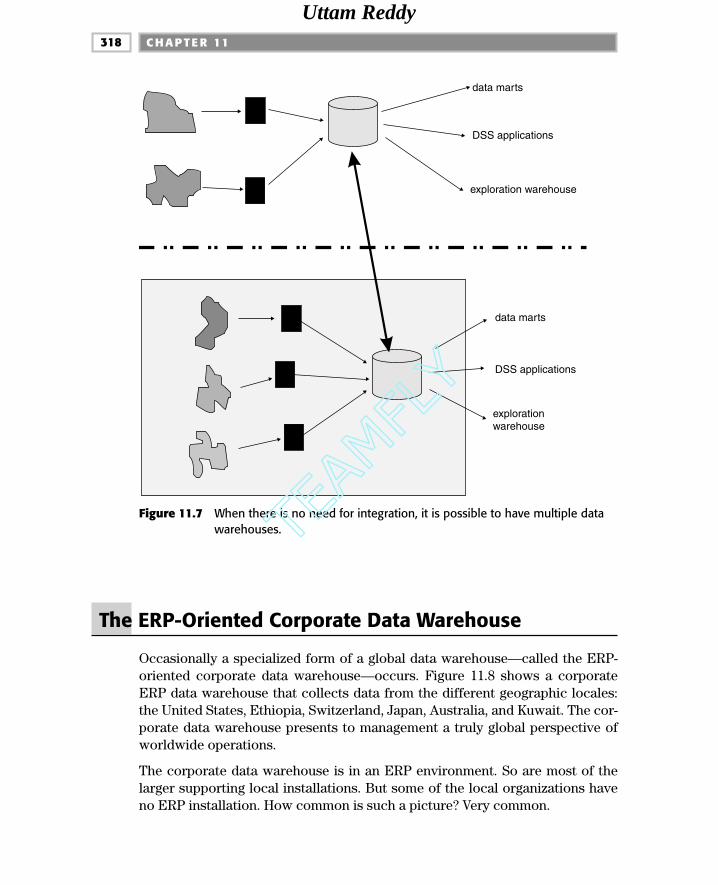
The ERP-Oriented Corporate Data Warehouse

Occasionally a specialized form of a global data warehouse—called the ERP-oriented corporate data warehouse—occurs. Figure 11.8 shows a corporateERP data warehouse that collects data from the different geographic locales:the United States, Ethiopia, Switzerland, Japan, Australia, and Kuwait. The cor-porate data warehouse presents to management a truly global perspective ofworldwide operations.

The corporate data warehouse is in an ERP environment. So are most of thelarger supporting local installations. But some of the local organizations haveno ERP installation. How common is such a picture? Very common.

C H A P T E R 11318

data marts

DSS applications

explorationwarehouse

data marts

DSS applications


Figure 11.7 When there is no need for integration, it is possible to have multiple datawarehouses. TE

AMFLY

Team-Fly®

Uttam Reddy

The first issue is getting data into the corporate ERP data warehouse. The dataneeds to be restructured and converted as it passes into the warehouse. Howeasy is the transition from the non-ERP installations to the corporate datawarehouse? Not particularly. And how easy is the passage of data from a localERP installation into the corporate ERP? Surprisingly difficult as well. The rea-son is that even though the local ERP installation may be in the same brand ofsoftware as the corporate ERP installation, there will nevertheless be many dif-ferences in the way the software has been implemented. Even if all of the localinstallations were in the same type of ERP, conversion to the headquartersinstallation would still be difficult.

Furthermore, one of the major challenges is keeping the headquarters datawarehouse in sync. Perhaps one day the rebels take over in Peru and lawschange. The headquarters data warehouse needs to be changed. The next day,a new discovery of oil is made in the Caribbean. More changes have to be madeto the corporate data warehouse. Next month, a new electronic device is madethat allows electricity generators to generate 10 times the power they once didwith no change in equipment. The headquarters data warehouse needs to be


corporateconsolidateddatawarehouse

U.S. ERP Ethiopianapplications Swiss

ERP

JapaneseERP Australian

ERPKuwaitiapplications(SAP) (SAP)

(SAP)

(PeopleSoft)

(BAAN)

Figure 11.8 An ERP-oriented rendition of the global data warehouse.

Uttam Reddy

changed again. Next month, there is an oil spill in Alaska, and the corporatedata warehouse needs to be changed yet again.

In short, there is a never-ending series of events that require the corporate datato be constantly changed. Building the corporate infrastructure to withstandthis eternal change is a significant challenge.

Summary

The ERP environment is an application-based environment found in manyplaces. Even with an ERP installation there is a need for a data warehouse. Thedeveloper has several choices, of which each have advantages and disadvan-tages:

■■ Move ERP data to a non-ERP data warehouse.

■■ Move ERP data to an ERP-based data warehouse.

■■ Move ERP data to an ERP-based data warehouse and move non-ERP datato a non-ERP–based data warehouse.

C H A P T E R 11320

Uttam Reddy

Data Warehouse Design Review Checklist

C H A P T E R 12

One of the most effective techniques for ensuring quality in the operational envi-ronment is the design review. Through design review, errors can be detectedand resolved prior to coding. The cost benefit of identifying errors early in thedevelopment life cycle is enormous.

In the operational environment, design review is usually done on completion ofthe physical design of an application. The types of issues around which an oper-ational design review centers are the following:

■■ Transaction performance

■■ Batch window adequacy

■■ System availability

■■ Capacity

■■ Project readiness

■■ User requirements satisfaction

Done properly in the operational environment, design review can save signifi-cant resources and greatly increase user satisfaction. Most importantly, whendesign review has been properly executed, major pieces of code do not have tobe torn up and rewritten after the system has gone into production.

321

Uttam Reddy

Design review is as applicable to the data warehouse environment as it is to theoperational environment, with a few provisos.

One proviso is that systems are developed in the data warehouse environmentin an iterative manner, where the requirements are discovered as a part of thedevelopment process. The classical operational environment is built under thewell-defined system development life cycle (SDLC). Systems in the data ware-house environment are not built under the SDLC. Other differences betweenthe development process in the operational environment and the data ware-house environment are the following:

■■ Development in the operational environment is done one application at atime. Systems for the data warehouse environment are built a subject areaat a time.

■■ In the operational environment, there is a firm set of requirements thatform the basis of operational design and development. In the data ware-house environment, there is seldom a firm understanding of processingrequirements at the outset of DSS development.

■■ In the operational environment, transaction response time is a major andburning issue. In the data warehouse environment, transaction responsetime had better not be an issue.

■■ In the operational environment, the input from systems usually comesfrom sources external to the organization, most often from interactionwith outside agencies. In the data warehouse environment, it usuallycomes from systems inside the organization where data is integrated froma wide variety of existing sources.

■■ In the operational environment, data is nearly all current valued (i.e., datais accurate as of the moment of use). In the data warehouse environment,data is time variant (i.e., data is relevant to some one moment in time).

There are, then, some substantial differences between the operational and datawarehouse environments, and these differences show up in the way designreview is conducted.

When to Do Design Review

Design review in the data warehouse environment is done as soon as a majorsubject area has been designed and is ready to be added to the data warehouseenvironment. It does not need to be done for every new database that goes up.Instead, as whole new major subject areas are added to the database, designreview becomes an appropriate activity.

C H A P T E R 12322

Uttam Reddy

Who Should Be in the Design Review?The attendees at the design review include anyone who has a stake in the devel-opment, operation, or use of the DSS subject area being reviewed.

Normally, this includes the following parties:

■■ The data administration (DA)

■■ The database administration (DBA)

■■ Programmers

■■ The DSS analysts

■■ End users other than the DSS analysts

■■ Operations

■■ Systems support

■■ Management

Of this group, by far the most important attendees are the end users and theDSS analysts.

One important benefit from having all the parties in the same room at the sametime is the opportunity to short-circuit miscommunications. In an everydayenvironment where the end user talks to the liaison person who talks to thedesigner who talks to the programmer, there is ample opportunity for miscom-munication and misinterpretation. When all the parties are gathered, direct con-versations can occur that are beneficial to the health of the project beingreviewed.

What Should the Agenda Be?The subject for review for the data warehouse environment is any aspect ofdesign, development, project management, or use that might prevent success.In short, any obstacle to success is relevant to the design review process. As a rule, the more controversial the subject, the more important that it beaddressed during the review.

The questions that form the basis of the review process are addressed in the lat-ter part of this chapter.

The ResultsA data warehouse design review has three results:

■■ An appraisal to management of the issues, and recommendations as to fur-ther action

Data Warehouse Design Review Checklist 323

Uttam Reddy

■■ A documentation of where the system is in the design, as of the moment ofreview

■■ An action item list that states specific objectives and activities that are aresult of the review process

Administering the ReviewThe review is led by two people—a facilitator and a recorder. The facilitator isnever the manager or the developer of the project being reviewed. If, by somechance, the facilitator is the project leader, the purpose of the review—frommany perspectives—will have been defeated.

To conduct a successful review, the facilitator must be someone removed fromthe project for the following reasons:

As an outsider, the facilitator provides an external perspective—a fresh look—at the system. This fresh look often reveals important insights that someoneclose to the design and development of the system is not capable of providing.

As an outsider, a facilitator can offer criticism constructively. The criticism thatcomes from someone close to the development effort is usually taken person-ally and causes the design review to be reduced to a very base level.

A Typical Data Warehouse Design Review

1. Who is missing in the review? Is any group missing that ought to be inattendance? Are the following groups represented?

■■ DA

■■ DBA

■■ Programming

■■ DSS analysts

■■ End users

■■ Operations

■■ Systems programming

■■ Auditing

■■ Management

Who is the official representative of each group?

ISSUE: The proper attendance at the design review by the proper people isvital to the success of the review regardless of any other factors. Easily, the

C H A P T E R 12324

Uttam Reddy

most important attendee is the DSS analyst or the end user. Managementmay or may not attend at their discretion.

2. Have the end-user requirements been anticipated at all? If so, to whatextent have they been anticipated? Does the end-user representative to thedesign review agree with the representation of requirements that has beendone?

ISSUE: In theory, the DSS environment can be built without interactionwith the end user—with no anticipation of end-user requirements. If therewill be a need to change the granularity of data in the data warehouse envi-ronment, or if EIS/artificial intelligence processing is to be built on top ofthe data warehouse, then some anticipation of requirements is a healthyexercise to go through. As a rule, even when the DSS requirements are antic-ipated, the level of participation of the end users is very low, and the endresult is very sketchy. Furthermore, a large amount of time should not beallocated to the anticipation of end-user requirements.

3. How much of the data warehouse has already been built in the data ware-house environment?

■■ Which subjects?

■■ What detail? What summarization?

■■ How much data—in bytes? In rows? In tracks/cylinders?

■■ How much processing?

■■ What is the growth pattern, independent of the project being reviewed?

ISSUE: The current status of the data warehouse environment has a greatinfluence on the development project being reviewed. The very first devel-opment effort should be undertaken on a limited-scope, trial-and-errorbasis. There should be little critical processing or data in this phase. In addi-tion, a certain amount of quick feedback and reiteration of developmentshould be anticipated.

Later efforts of data warehouse development will have smaller margins forerror.

4. How many major subjects have been identified from the data model? Howmany are currently implemented? How many are fully implemented? Howmany are being implemented by the development project being reviewed?How many will be implemented in the foreseeable future?

ISSUE: As a rule, the data warehouse environment is implemented one sub-ject at a time. The first few subjects should be considered almost as experi-ments. Later subject implementation should reflect the lessons learned fromearlier development efforts.


Uttam Reddy

5. Does any major DSS processing (i.e., data warehouse) exist outside thedata warehouse environment? If so, what is the chance of conflict or over-lap? What migration plan is there for DSS data and processing outside thedata warehouse environment? Does the end user understand the migrationthat will have to occur? In what time frame will the migration be done?

ISSUE: Under normal circumstances, it is a major mistake to have only partof the data warehouse in the data warehouse environment and other partsout of the data warehouse environment. Only under the most exceptionalcircumstances should a “split” scenario be allowed. (One of those circum-stances is a distributed DSS environment.)

If part of the data warehouse, in fact, does exist outside the data warehouseenvironment, there should be a plan to bring that part of the DSS world backinto the data warehouse environment.

6. Have the major subjects that have been identified been broken down intolower levels of detail?

■■ Have the keys been identified?

■■ Have the attributes been identified?

■■ Have the keys and attributes been grouped together?

■■ Have the relationships between groupings of data been identified?

■■ Have the time variances of each group been identified?

ISSUE: There needs to be a data model that serves as the intellectual heartof the data warehouse environment. The data model normally has threelevels—a high-level model where entities and relationships are identified; amidlevel where keys, attributes, and relationships are identified; and a lowlevel, where database design can be done. While not all of the data needs tobe modeled down to the lowest level of detail in order for the DSS environ-ment to begin to be built, at least the high-level model must be complete.

7. Is the design discussed in question 6 periodically reviewed? (How often?Informally? Formally?) What changes occur as a result of the review? Howis end-user feedback channeled to the developer?

ISSUE: From time to time, the data model needs to be updated to reflectchanging business needs of the organization. As a rule, these changes areincremental in nature. It is very unusual to have a revolutionary change.There needs to be an assessment of the impact of these changes on bothexisting data warehouse data and planned data warehouse data.

8. Has the operational system of record been identified?

■■ Has the source for every attribute been identified?

■■ Have the conditions under which one attribute or another will be thesource been identified?

C H A P T E R 12326

Uttam Reddy

■■ If there is no source for an attribute, have default values been identified?

■■ Has a common measure of attribute values been identified for thosedata attributes in the data warehouse environment?

■■ Has a common encoding structure been identified for those attributesin the data warehouse environment?

■■ Has a common key structure in the data warehouse environment beenidentified? Where the system of record key does not meet the condi-tions for the DSS key structure, has a conversion path been identified?

■■ If data comes from multiple sources, has the logic to determine theappropriate value been identified?

■■ Has the technology that houses the system of record been identified?

■■ Will any attribute have to be summarized on entering the data ware-house?

■■ Will multiple attributes have to be aggregated on entering the datawarehouse?

■■ Will data have to be resequenced on passing into the data warehouse?

ISSUE: After the data model has been built, the system of record is identi-fied. The system of record normally resides in the operational environment.The system of record represents the best source of existing data in supportof the data model. The issues of integration are very much a factor in defin-ing the system of record.

9. Has the frequency of extract processing—from the operational system ofrecord to the data warehouse environment—been identified? How will theextract processing identify changes to the operational data from the lasttime an extract process was run?

■■ By looking at time-stamped data?

■■ By changing operational application code?

■■ By looking at a log file? An audit file?

■■ By looking at a delta file?

■■ By rubbing “before” and “after” images together?

ISSUE: The frequency of extract processing is an issue because of theresources required in refreshment, the complexity of refreshment process-ing, and the need to refresh data on a timely basis. The usefulness of datawarehouse data is often related to how often the data warehouse data isrefreshed.

One of the most complex issues—from a technical perspective—is deter-mining what data is to be scanned for extract processing. In some cases, theoperational data that needs to pass from one environment to the next is


Uttam Reddy

straightforward. In other cases, it is not clear at all just what data should beexamined as a candidate for populating the data warehouse environment.

10. What volume of data will normally be contained in the DSS environment?If the volume of data is large,

■■ Will multiple levels of granularity be specified?

■■ Will data be compacted?

■■ Will data be purged periodically?

■■ Will data be moved to near-line storage? At what frequency?

ISSUE: In addition to the volumes of data processed by extraction, thedesigner needs to concern himself or herself with the volume of data actu-ally in the data warehouse environment. The analysis of the volume of datain the data warehouse environment leads directly to the subject of the gran-ularity of data in the data warehouse environment and the possibility of mul-tiple levels of granularity.

11. What data will be filtered out of the operational environment as extractprocessing is done to create the data warehouse environment?

ISSUE: It is very unusual for all operational data to be passed to the DSSenvironment. Almost every operational environment contains data that isrelevant only to the operational environment. This data should not bepassed to the data warehouse environment.

12. What software will be used to feed the data warehouse environment?

■■ Has the software been thoroughly shaken out?

■■ What bottlenecks are there or might there be?

■■ Is the interface one-way or two-way?

■■ What technical support will be required?

■■ What volume of data will pass through the software?

■■ What monitoring of the software will be required?

■■ What alterations to the software will be periodically required?

■■ What outage will the alterations entail?

■■ How long will it take to install the software?

■■ Who will be responsible for the software?

■■ When will the software be ready for full-blown use?

ISSUE: The data warehouse environment is capable of handling a largenumber of different types of software interfaces. The amount of break-intime and “infrastructure” time, however, should not be underestimated. TheDSS architect must not assume that the linking of the data warehouse envi-

C H A P T E R 12328

TEAMFLY

Team-Fly®

Uttam Reddy

ronment to other environments will necessarily be straightforward andeasy.

13. What software/interface will be required for the feeding of DSS departmen-tal and individual processing out of the data warehouse environment?

■■ Has the interface been thoroughly tested?

■■ What bottlenecks might exist?

■■ Is the interface one-way or two-way?

■■ What technical support will be required?

■■ What traffic of data across the interface is anticipated?

■■ What monitoring of the interface will be required?

■■ What alterations to the interface will there be?

■■ What outage is anticipated as a result of alterations to the interface?

■■ How long will it take to install the interface?

■■ Who will be responsible for the interface?

■■ When will the interface be ready for full-scale utilization?

14. What physical organization of data will be used in the data warehouse envi-ronment? Can the data be directly accessed? Can it be sequentiallyaccessed? Can indexes be easily and cheaply created?

ISSUE: The designer needs to review the physical configuration of the datawarehouse environment to ensure that adequate capacity will be availableand that the data, once in the environment, will be able to be manipulated ina responsive manner.

15. How easy will it be to add more storage to the data warehouse environ-ment at a later point in time? How easy will it be to reorganize data withinthe data warehouse environment at a later point in time?

ISSUE: No data warehouse is static, and no data warehouse is fully speci-fied at the initial moment of design. It is absolutely normal to make correc-tions in design throughout the life of the data warehouse environment. Toconstruct a data warehouse environment either where midcourse correc-tions cannot be made or are awkward to make is to have a faulty design.

16. What is the likelihood that data in the data warehouse environment willneed to be restructured frequently (i.e., columns added, dropped, orenlarged, keys modified, etc.)? What effect will these activities of restruc-turing have on ongoing processing in the data warehouse?

ISSUE: Given the volume of data found in the data warehouse environment,restructuring it is not a trivial issue. In addition, with archival data, restruc-turing after a certain moment in time often becomes a logical impossibility.


Uttam Reddy

17. What are the expected levels of performance in the data warehouse envi-ronment? Has a DSS service level agreement been drawn up either for-mally or informally?

ISSUE: Unless a DSS service-level agreement has been formally drawn up,it is impossible to measure whether performance objectives are being met.The DSS service level agreement should cover both DSS performance levelsand downtime. Typical DSS service level agreements state such things as thefollowing:

■■ Average performance during peak hours per units of data

■■ Average performance during off-peak hours per units of data

■■ Worst performance levels during peak hours per units of data

■■ Worst performance during off-peak hours per units of data

■■ System availability standards

One of the difficulties of the DSS environment is measuring performance.Unlike the operational environment where performance can be measured inabsolute terms, DSS processing needs to be measured in relation to thefollowing:

■■ How much processing the individual request is for

■■ How much processing is going on concurrently

■■ How many users are on the system at the moment of execution

18. What are the expected levels of availability? Has an availability agreementbeen drawn up for the data warehouse environment, either formally orinformally?

ISSUE: (See issue for question 17.)

19. How will the data in the data warehouse environment be indexed oraccessed?

■■ Will any table have more than four indexes?

■■ Will any table be hashed?

■■ Will any table have only the primary key indexed?

■■ What overhead will be required to maintain the index?

■■ What overhead will be required to load the index initially?

■■ How often will the index be used?

■■ Can/should the index be altered to serve a wider use?

ISSUE: Data in the data warehouse environment needs to be able to beaccessed efficiently and in a flexible manner. Unfortunately, the heuristic

C H A P T E R 12330

Uttam Reddy

nature of data warehouse processing is such that the need for indexes isunpredictable. The result is that the accessing of data in the data warehouseenvironment must not be taken for granted. As a rule, a multitieredapproach to managing the access of data warehouse data is optimal:

■■ The hashed/primary key should satisfy most accesses.

■■ Secondary indexes should satisfy other popular access patterns.

■■ Temporary indexes should satisfy the occasional access.

■■ Extraction and subsequent indexing of a subset of data warehouse datashould satisfy infrequent or once-in-a-lifetime accesses of data.

In any case, data in the data warehouse environment should not be stored inpartitions so large that they cannot be indexed freely.

20. What volumes of processing in the data warehouse environment are to beexpected? What about peak periods? What will the profile of the averageday look like? The peak rate?

ISSUE: Not only should the volume of data in the data warehouse environ-ment be anticipated, but the volume of processing should be anticipated aswell.

21. What level of granularity of data in the data warehouse environment willthere be?

■■ A high level?

■■ A low level?

■■ Multiple levels?

■■ Will rolling summarization be done?

■■ Will there be a level of true archival data?

■■ Will there be a living sample level of data?

ISSUE: Clearly, the most important design issue in the data warehouse envi-ronment is that of granularity of data and the possibility of multiple levels ofgranularity. In a word, if the granularity of the data warehouse environmentis done properly, then all other issues become straightforward; if the granu-larity of data in the data warehouse environment is not designed properly,then all other design issues become complex and burdensome.

22. What purge criteria for data in the data warehouse environment will therebe? Will data be truly purged, or will it be compacted and archived else-where? What legal requirements are there? What audit requirements arethere?

ISSUE: Even though data in the DSS environment is archival and of neces-sity has a low probability of access, it nevertheless has some probability of


Uttam Reddy

access (otherwise it should not be stored). When the probability of accessreaches zero (or approaches zero), the data needs to be purged. Given thatvolume of data is one of the most burning issues in the data warehouseenvironment, purging data that is no longer useful is one of the moreimportant aspects of the data warehouse environment.

23. What total processing capacity requirements are there:

■■ For initial implementation?

■■ For the data warehouse environment at maturity?

ISSUE: Granted that capacity requirements cannot be planned down to thelast bit, it is worthwhile to at least estimate how much capacity will berequired, just in case there is a mismatch between needs and what will beavailable.

24. What relationships between major subject areas will be recognized in thedata warehouse environment? Will their implementation do the following:

■■ Cause foreign keys to be kept up-to-date?

■■ Make use of artifacts?

What overhead is required in the building and maintenance of the relation-ship in the data warehouse environment?

ISSUE: One of the most important design decisions the data warehousedesigner makes is that of how to implement relationships between data inthe data warehouse environment. Data relationships are almost neverimplemented the same way in the data warehouse as they are in the opera-tional environment.

25. Do the data structures internal to the data warehouse environment makeuse of the following:

■■ Arrays of data?

■■ Selective redundancy of data?

■■ Merging of tables of data?

■■ Creation of commonly used units of derived data?

ISSUE: Even though operational performance is not an issue in the datawarehouse environment, performance is nevertheless an issue. Thedesigner needs to consider the design techniques listed previously whenthey can reduce the total amount of I/O consumed. The techniques listedpreviously are classical physical denormalization techniques. Because datais not updated in the data warehouse environment, there are very fewrestrictions on what can and can’t be done.

C H A P T E R 12332

Uttam Reddy

The factors that determine when one or the other design technique can beused include the following:

■■ The predictability of occurrences of data

■■ The predictability of the pattern of access of data

■■ The need to gather artifacts of data

26. How long will a recovery take? Is computer operations prepared to exe-cute a full data warehouse database recovery? A partial recovery? Willoperations periodically practice recovery so that it will be prepared in theevent of a need for recovery? What level of preparedness is exhibited bythe following:

■■ Systems support?

■■ Applications programming?

■■ The DBA?

■■ The DA?

For each type of problem that can arise, is it clear whose responsibility theproblem is?

ISSUE: As in operational systems, the designer must be prepared for theoutages that occur during recovery. The frequency of recovery, the length oftime required to bring the system back up, and the domino effect that canoccur during an outage must all be considered.

Have instructions been prepared, tested, and written? Have these instruc-tions been kept up-to-date?

27. What level of preparation is there for reorganization/restructuring of:

■■ Operations?



■■ The DBA?

■■ The DA?

Have written instructions and procedures been set and tested? Are they up-to-date? Will they be kept up-to-date?

ISSUE: (See issues for question 26.)

28. What level of preparation is there for the loading of a database table by:

■■ Operations?




Uttam Reddy

■■ The DBA?

■■ The DA?

Have written instructions and procedures been made and tested? Are theyup-to-date? Will they be kept up-to-date?

ISSUE: The time and resources for loading can be considerable. This esti-mate needs to be made carefully and early in the development life cycle.

29. What level of preparation is there for the loading of a database index by:

■■ Operations?



■■ The DBA?

■■ The DA?


30. If there is ever a controversy as to the accuracy of a piece of data in thedata warehouse environment, how will the conflict be resolved? Has own-ership (or at least source identification) been done for each unit of data inthe data warehouse environment? Will ownership be able to be establishedif the need arises? Who will address the issues of ownership? Who will bethe final authority as to the issues of ownership?

ISSUE: Ownership or stewardship of data is an essential component of suc-cess in the data warehouse environment. It is inevitable that at somemoment in time the contents of a database will come into question. Thedesigner needs to plan in advance for this eventuality.

31. How will corrections to data be made once data is placed in the data ware-house environment? How frequently will corrections be made? Will correc-tions be monitored? If there is a pattern of regularly occurring changes,how will corrections at the source (i.e., operational) level be made?

ISSUE: On an infrequent, nonscheduled basis, there may need to bechanges made to the data warehouse environment. If there appears to be apattern to these changes, then the DSS analyst needs to investigate what iswrong in the operational system.

32. Will public summary data be stored separately from normal primitive DSSdata? How much public summary data will there be? Will the algorithmrequired to create public summary data be stored?

ISSUE: Even though the data warehouse environment contains primitivedata, it is normal for there to be public summary data in the data warehouse

C H A P T E R 12334

Uttam Reddy

environment as well. The designer needs to have prepared a logical place forthis data to reside.

33. What security requirements will there be for the databases in the datawarehouse environment? How will security be enforced?

ISSUE: The access of data becomes an issue, especially as the detailed databecomes summarized or aggregated, where trends become apparent. Thedesigner needs to anticipate the security requirements and prepare the datawarehouse environment for them.

34. What audit requirements are there? How will audit requirements be met?

ISSUE: As a rule, system audit can be done at the data warehouse level, butthis is almost always a mistake. Instead, detailed record audits are best doneat the system-of-record level.

35. Will compaction of data be used? Has the overhead of compacting/decom-pacting data been considered? What is the overhead? What are the savingsin terms of DASD for compacting/decompacting data?

ISSUE: On one hand, compaction or encoding of data can save significantamounts of space. On the other hand, both compacting and encoding datarequire CPU cycles as data is decompacted or decoded on access. Thedesigner needs to make a thorough investigation of these issues and a delib-erate trade-off in the design.

36. Will encoding of data be done? Has the overhead of encoding/decodingbeen considered? What, in fact, is the overhead?


37. Will meta data be stored for the data warehouse environment?

ISSUE: Meta data needs to be stored with any archival data as a matter ofpolicy. There is nothing more frustrating than an analyst trying to solve aproblem using archival data when he or she does not know the meaning ofthe contents of a field being analyzed. This frustration can be alleviated bystoring the semantics of data with the data as it is archived. Over time, it isabsolutely normal for the contents and structure of data in the data ware-house environment to change. Keeping track of the changing definition ofdata is something the designer should make sure is done.

38. Will reference tables be stored in the data warehouse environment?


39. What catalog/dictionary will be maintained for the data warehouse envi-ronment? Who will maintain it? How will it be kept up-to-date? To whomwill it be made available?


Uttam Reddy

ISSUE: Not only is keeping track of the definition of data over time an issue,but keeping track of data currently in the data warehouse is important aswell.

40. Will update (as opposed to loading and access of data) be allowed in thedata warehouse environment? (Why? How much? Under what circum-stances? On an exception-only basis?)

ISSUE: If any updating is allowed on a regular basis in the data warehouseenvironment, the designer should ask why. The only update that shouldoccur should be on an exception basis and for only small amounts of data.Any exception to this severely compromises the efficacy of the data ware-house environment.

When updates are done (if, in fact, they are done at all), they should be runin a private window when no other processing is done and when there isslack time on the processor.

41. What time lag will there be in getting data from the operational to the datawarehouse environment? Will the time lag ever be less than 24 hours? If so,why and under what conditions? Will the passage of data from the opera-tional to the data warehouse environment be a “push” or a “pull” process?

ISSUE: As a matter of policy, any time lag less than 24 hours should be ques-tioned. As a rule, if a time lag of less than 24 hours is required, it is a sign thatthe developer is building operational requirements into the data warehouse.The flow of data through the data warehouse environment should always bea pull process, where data is pulled into the warehouse environment whenit is needed, rather than being pushed into the warehouse environmentwhen it is available.

42. What logging of data warehouse activity will be done? Who will haveaccess to the logs?

ISSUE: Most DSS processing does not require logging. If an extensiveamount of logging is required, it is usually a sign of lack of understanding ofwhat type of processing is occurring in the data warehouse environment.

43. Will any data other than public summary data flow to the data warehouseenvironment from the departmental or individual level? If so, describe it.

ISSUE: Only on rare occasions should public summary data come fromsources other than departmental or individual levels of processing. If muchpublic summary data is coming from other sources, the analyst should askwhy.

44. What external data (i.e., data other than that generated by a company’sinternal sources and systems) will enter the data warehouse environment?Will it be specially marked? Will its source be stored with the data? How

C H A P T E R 12336

Uttam Reddy

frequently will the external data enter the system? How much of it willenter? Will an unstructured format be required? What happens if the exter-nal data is found to be inaccurate?

ISSUE: Even though there are legitimate sources of data other than a com-pany’s operational systems, if much data is entering externally, the analystshould ask why. Inevitably, there is much less flexibility with the contentand regularity of availability of external data, although external data repre-sents an important resource that should not be ignored.

45. What facilities will exist that will help the departmental and the individualuser to locate data in the data warehouse environment?

ISSUE: One of the primary features of the data warehouse is ease of acces-sibility of data. And the first step in the accessibility of data is the initial loca-tion of the data.

46. Will there be an attempt to mix operational and DSS processing on thesame machine at the same time? (Why? How much processing? How muchdata?)

ISSUE: For a multitude of reasons, it makes little sense to mix operationaland DSS processing on the same machine at the same time. Only wherethere are small amounts of data and small amounts of processing shouldthere be a mixture. But these are not the conditions under which the datawarehouse environment is most cost-effective. (See my previous book Data

Architecture: The Information Paradigm [QED/Wiley, 1992] for an in-depthdiscussion of this issue.)

47. How much data will flow back to the operational level from the data ware-house level? At what rate? At what volume? Under what response timeconstraints? Will the flowback be summarized data or individual units ofdata?

ISSUE: As a rule, data flows from the operational to the warehouse level tothe departmental to the individual levels of processing. There are somenotable exceptions. As long as not too much data “backflows,” and as longas the backflow is done in a disciplined fashion, there usually is no problem.If there is a lot of data engaged in backflow, then a red flag should be raised.

48. How much repetitive processing will occur against the data warehouseenvironment? Will precalculation and storage of derived data save process-ing time?

ISSUE: It is absolutely normal for the data warehouse environment to havesome amount of repetitive processing done against it. If only repetitive pro-cessing is done, however, or if no repetitive processing is planned, thedesigner should question why.


Uttam Reddy

49. How will major subjects be partitioned? (By year? By geography? By func-tional unit? By product line?) Just how finely does the partitioning of thedata break the data up?

ISSUE: Given the volume of data that is inherent to the data warehouseenvironment and the unpredictable usage of the data, it is mandatory thatdata warehouse data be partitioned into physically small units that can bemanaged independently. The design issue is not whether partitioning is to bedone. Instead, the design issue is how partitioning is to be accomplished. Ingeneral, partitioning is done at the application level rather than the systemlevel.

The partitioning strategy should be reviewed with the following in mind:

■■ Current volume of data

■■ Future volume of data

■■ Current usage of data

■■ Future usage of data

■■ Partitioning of other data in the warehouse

■■ Use of other data

■■ Volatility of the structure of data

50. Will sparse indexes be created? Would they be useful?

ISSUE: Sparse indexes created in the right place can save huge amounts ofprocessing. By the same token, sparse indexes require a fair amount of over-head in their creation and maintenance. The designer of the data warehouseenvironment should consider their use.

51. What temporary indexes will be created? How long will they be kept? Howlarge will they be?

ISSUE: (See the issue for question 50, except as it applies to temporaryindexes.)

52. What documentation will there be at the departmental and individual lev-els? What documentation will there be of the interfaces between the datawarehouse environment and the departmental environment? Between thedepartmental and the individual environment? Between the data ware-house environment and the individual environment?

ISSUE: Given the free-form nature of processing in the departmental andthe individual environments, it is unlikely that there will be much in the wayof available documentation. A documentation of the relationships betweenthe environments is important for the reconcilability of data.

C H A P T E R 12338

TEAMFLY

Team-Fly®

Uttam Reddy

53. Will the user be charged for departmental processing? For individual pro-cessing? Who will be charged for data warehouse processing?

ISSUE: It is important that users have their own budgets and be charged forresources used. The instant that processing becomes “free,” it is predictablethat there will be massive misuse of resources. A chargeback system instillsa sense of responsibility in the use of resources.

54. If the data warehouse environment is to be distributed, have the commonparts of the warehouse been identified? How are they to be managed?

ISSUE: In a distributed data warehouse environment, some of the data willnecessarily be tightly controlled. The data needs to be identified up front bythe designer and meta data controls put in place.

55. What monitoring of the data warehouse will there be? At the table level? Atthe row level? At the column level?

ISSUE: The use of data in the warehouse needs to be monitored to deter-mine the dormancy rate. Monitoring must occur at the table level, the rowlevel, and the column level. In addition, monitoring of transaction needs tooccur as well.

56. Will class IV ODS be supported? How much performance impact will therebe on the data warehouse to support class IV ODS processing?

ISSUE: Class IV ODS is fed from the data warehouse. The data needed tocreate the profile in the class IV ODS is found in the data warehouse.

57. What testing facility will there be for the data warehouse?

ISSUE: Testing in the data warehouse is not the same level of importance asin the operational transaction environment. But occasionally there is a needfor testing, especially when new types of data are being loaded and whenthere are large volumes of data.

58. What DSS applications will be fed from the data warehouse? How muchvolume of data will be fed?

ISSUE: DSS applications, just like data marts, are fed from the data ware-house. There are the issues of when the data warehouse will be examined,how often it will be examined, and what performance impact there will bebecause for the analysis.

59. Will an exploration warehouse and/or a data mining warehouse be fedfrom the data warehouse? If not, will exploration processing be donedirectly in the data warehouse? If so, what resources will be required tofeed the exploration/data mining warehouse?


Uttam Reddy

ISSUE: The creation of an exploration warehouse and/or a data mining datawarehouse can greatly alleviate the resource burden on the data warehouse.An exploration warehouse is needed when the frequency of exploration issuch that statistical analysis starts to have an impact on data warehouseresources.

The issues here are the frequency of update and the volume of data thatneeds to be updated. In addition, the need for an incremental update of thedata warehouse occasionally arises.

60. What resources are required for loading data into the data warehouse onan ongoing basis? Will the load be so large that it cannot fit into the win-dow of opportunity? Will the load have to be parallelized?

ISSUE: Occasionally there is so much data that needs to be loaded into thedata warehouse that the window for loading is not large enough. When theload is too large there are several options:

■■ Creating a staging area where much preprocessing of the data to beloaded can be done independently

■■ Parallelizing the load stream so that the elapsed time required for load-ing is shrunk to the point that the load can be done with normal pro-cessing

■■ Editing or summarizing the data to be loaded so that the actual load issmaller

61. To what extent has the midlevel model of the subject areas been created?Is there a relationship between the different midlevel models?

ISSUE: Each major subject area has its own midlevel data model. As a rulethe midlevel data models are created only as the iteration of developmentneeds to have them created. In addition, the midlevel data models arerelated in the same way that the major subject areas are related.

62. Is the level of granularity of the data warehouse sufficiently low enough inorder to service all the different architectural components that will be fedfrom the data warehouse?

ISSUE: The data warehouse feeds many different architectural compo-nents. The level of granularity of the data warehouse must be sufficientlylow to feed the lowest level of data needed anywhere in the corporate infor-mation factory. This is why it is said that the data in the data warehouse is atthe lowest common denominator.

63. If the data warehouse will be used to store ebusiness and clickstream data,to what extent does the Granularity Manager filter the data?

C H A P T E R 12340

Uttam Reddy

ISSUE: The Web-based environment generates a huge amount of data. Thedata that is generated is at much too low a level of granularity. In order tosummarize and aggregate the data before entering the data warehouse, thedata is passed through a Granularity Manager. The Granularity Managergreatly reduces the volume of data that finds its way into the data ware-house.

64. What dividing line is used to determine what data is to be placed on diskstorage and what data is to be placed on alternate storage?

ISSUE: The general approach that most organizations take in the place-ment of data on disk storage and data on alternate storage is to place themost current data on disk storage and to place older data on alternate stor-age. Typically, disk storage may hold two years’ worth of data, and alternatestorage may hold all data that is older than two years.

65. How will movement of data to and from disk storage and alternate storagebe managed?

ISSUE: Most organizations have software that manages the traffic to andfrom alternate storage. The software is commonly known as a cross-mediastorage manager.

66. If the data warehouse is a global data warehouse, what data will be storedlocally and what data will be stored globally?

ISSUE: When a data warehouse is global, some data is stored centrally andother data is stored locally. The dividing line is determined by the use of thedata.

67. For a global data warehouse, is there assurance that data can be trans-ported across international boundaries?

ISSUE: Some countries have laws that do not allow data to pass beyondtheir boundaries. The data warehouse that is global must ensure that it is notin violation of international laws.

68. For ERP environments, has it been determined where the data warehousewill be located—inside the ERP software or outside the ERP environment?

ISSUE: Many factors determine where the data warehouse should beplaced:

■■ Does the ERP vendor support data warehouse?

■■ Can non-ERP data be placed inside the data warehouse?

■■ What analytical software can be used on the data warehouse if the datawarehouse is placed inside the ERP environment?

■■ If the data warehouse is placed inside the ERP environment, whatDBMS can be used?


Uttam Reddy

69. Can alternate storage be processed independently?

ISSUE: Older data is placed in alternate storage. It is often quite useful to beable to process the data found in alternate storage independently of any con-sideration of data placed on disk storage.

70. Is the development methodology that is being used for development a spi-ral development approach or a classical waterfall approach?

ISSUE: The spiral development approach is always the correct develop-ment approach for the data warehouse environment. The waterfall SDLCapproach is never the appropriate approach.

71. Will an ETL tool be used for moving data from the operational environmentto the data warehouse environment, or will the transformation be donemanually?

ISSUE: In almost every case, using a tool of automation to transform datainto the data warehouse environment makes sense. Only where there is avery small amount of data to be loaded into the data warehouse environ-ment should the loading of the data warehouse be done manually.

Summary

Design review is an important quality assurance practice that can greatlyincrease the satisfaction of the user and reduce development and maintenancecosts. Thoroughly reviewing the many aspects of a warehouse environmentprior to building the warehouse is a sound practice.

The review should focus on both detailed design and architecture.

C H A P T E R 12342

Uttam Reddy

Installing Custom Controls 343A P P E N D I X

DEVELOPING OPERATIONAL SYSTEMS—METH 1

M1—Initial Project Activities

PRECEDING ACTIVITY: Decision to build an operational system.

FOLLOWING ACTIVITY: Preparing to use existing code/data.

TIME ESTIMATE: Indeterminate, depending on size of project.

NORMALLY EXECUTED ONCE OR MULTIPLE TIMES: Once.

SPECIAL CONSIDERATIONS: Because of the ambiguity of this step, it tends todrag out interminably. As long as 90 percent (or even less) of the system isdefined here, the system development should continue into the next phase.

DELIVERABLE: Raw system requirements.

Interviews. The output of interviews is the “softcore” description of what thesystem is to do, usually reflecting the opinion of middle management. The for-mat of the output is very free-form. As a rule, the territory covered by inter-views is not comprehensive.

343

Uttam Reddy

Data gathering. The output from this activity may come from many sources.In general, requirements-usually detailed-that are not caught elsewhere aregathered here. This is a free-form, catchall, requirements-gathering activity, theresults of which fill in the gap for other requirements-gathering activities.

JAD (Joint Application Design) session output. The output from theseactivities is the group “brainstorm” synopsis. Some of the benefits of require-ments formulation in a JAD session are the spontaneity and flow of ideas, andthe critical mass that occurs by having different people in the same room focus-ing on a common objective. The output of one or more JAD sessions is a for-malized set of requirements that collectively represent the end users’ needs.

Strategic business plan analysis. If the company has a strategic businessplan, it makes sense to reflect on how the plan relates to the requirements ofthe system being designed. The influence of the strategic business plan canmanifest itself in many ways-in setting growth figures, in identifying new linesof business, in describing organizational changes, and so forth. All of these fac-tors, and more, shape the requirements of the system being built.

Existing systems shape requirements for a new system profoundly. If related,existing systems have been built, at the very least the interface between thenew set of requirements and existing systems must be identified.

Conversion, replacement, parallel processing, and so forth are all likely topics.The output of this activity is a description of the impact and influence of exist-ing systems on the requirements for the system being developed.

PARAMETERS OF SUCCESS: When done properly, there is a reduction inthe ambiguity of the system, the scope of the development effort is reasonablyset, and the components of the system are well organized. The political as wellas the technical components of the system should be captured and defined.

M2—Using Existing Code/Data

PRECEDING ACTIVITY: System definition.

FOLLOWING ACTIVITY: Sizing, phasing.

TIME ESTIMATE: Done very quickly, usually in no more than a week in eventhe largest of designs.


SPECIAL CONSIDERATIONS: This step is one of the best ways to ensure codereusability and data reusability. This step is crucial to the integration of theenvironment.

A P P E N D I X344

Uttam Reddy

In an architected environment, it is incumbent on every project to do the fol-lowing:

■■ Use as much existing code/data as possible.

■■ Prepare for future projects that will use code and data to be developed inthe current project. The output from this step is an identification of exist-ing code/data that can be reused and the steps that need to be taken forfuture processing.

If existing code/data is to be modified, the modifications are identified as a reg-ular part of the system development requirements. If existing code/data is to bedeleted, the deletion becomes a part of the specifications. If conversion ofcode/data are to be done, the conversion becomes a component of the devel-opment effort.

PARAMETERS OF SUCCESS: To identify code/data that already exists thatcan be built on; to identify what needs to be built to prepare for future efforts.

M3—Sizing, Phasing

PRECEDING ACTIVITY: Using existing code/data.

FOLLOWING ACTIVITY: Requirements formalization; capacity analysis.

TIME ESTIMATE: This step goes rapidly, usually in a day or two, even for thelargest of designs.

NORMALLY EXECUTED ONCE OR MULTIPLE TIMES: Once, then revisited foreach continuing phase of development.

DELIVERABLE: Identification of phases of development.

After the general requirements are gathered, the next step is to size them anddivide development up into phases. If the system to be developed is large, itmakes sense to break it into development phases. In doing so, development isparceled out in small, manageable units. Of course, the different developmentphases must be organized into a meaningful sequence, so that the second phasebuilds on the first, the third phase builds on the first and second, and so on.

The output from this step is the breakup of general requirements into doable,manageable phases, if the requirements are large enough to require a breakupat all.

PARAMETERS OF SUCCESS: To continue the development process inincrements that are both economic and doable (and within the political contextof the organization as well).

APPENDIX 345

Uttam Reddy

M4—Requirements Formalization

PRECEDING ACTIVITY: Sizing, phasing.

FOLLOWING ACTIVITY: ERD specification; functional decomposition.

TIME ESTIMATE: Indeterminate, depending on size of system, how well thescope of the system has been defined, and how ambiguous the design is up tothis point.

NORMALLY EXECUTED ONCE OR MULTIPLE TIMES: Once per phase ofdevelopment.

DELIVERABLE: Formal requirements specification.

Once the requirements have been gathered, sized, and phased (if necessary),the next step is to formalize them. In this step, the developer ensures the fol-lowing:

■■ The requirements that have been gathered are complete, as far as it is rea-sonably possible to gather them.

■■ The requirements are organized.

■■ The requirements are readable, comprehensible, and at a low enough levelof detail to be effective.

■■ The requirements are not in conflict with each other.

■■ The requirements do not overlap.

■■ Operational and DSS requirements have been separated.

■■ The output from this step is a formal requirements definition that is readyto go to detailed design.

PARAMETERS OF SUCCESS: A succinct, organized, readable, doable, quan-tified, complete, usable set of requirements that is also a document for devel-opment.

CA—Capacity Analysis

PRECEDING ACTIVITY: Sizing, phasing.

FOLLOWING ACTIVITY: ERD specification; functional decomposition.

TIME ESTIMATE: Depends on the size of the system being built, but with esti-mating tools and a focused planner, two or three weeks is a reasonable estimatefor a reasonably sized system.

A P P E N D I X346

Uttam Reddy


SPECIAL CONSIDERATIONS: The capacity planning function has a history ofconfusing issues and including extraneous factors that do not merit specialattention. It is important to keep the capacity planning portion of the develop-ment process focused and to the point. Otherwise, the exercise can become aroadblock to progress.

The gross amounts of resources to be consumed by the project being analyzedneed to be estimated in this early phase of development. In particular, the fol-lowing needs to be considered:

■■ DASD consumption

■■ Software requirements (including system software, utilities, special customcode, network software, interface software)

■■ CPU consumption

■■ I/O utilization

■■ Main memory requirements

■■ Network/channel utilization

Not only are raw requirements analyzed, but the arrival rate of transactions,peak-period processing, patterns of processing, response time requirements,availability requirements, and mean time to failure requirements are factored inas well.

In addition, if any hardware/software must be ordered, the lead time and the“burn in” time must be accounted for to ensure that proper resources will be inplace in time for the application being reviewed.

The output of this phase of development is the assurance that the resourcesneeded to be in place are, in fact, in place.

PARAMETERS OF SUCCESS: No surprises when it comes to resourcesbeing in place when needed, the lead time needed to acquire resources, and theamount of resources needed.

PREQ1—Technical EnvironmentDefinition

PRECEDING ACTIVITY: Establishment of the information processing environ-ment.

FOLLOWING ACTIVITY: Sizing, phasing.

APPENDIX 347

Uttam Reddy

TIME ESTIMATE: NA

NORMALLY EXECUTED ONCE OR MULTIPLE TIMES: NA

SPECIAL CONSIDERATIONS: On occasion, it is necessary to build an applica-tion system from scratch, including defining the technical environment. If thisis the case, the considerations of technical definition are outside the bound-aries of the data-driven development methodology.

In order to proceed, it is necessary that the technical environment be defined.If the technical environment is not defined at this point, the result will be much“thrashing.” Simply stated, detailed design cannot be meaningfully done untilthe technical environment is defined.

Certain elements of design beyond this point depend on one or the other of thetechnical cornerstones previously identified. At the least, the following shouldbe established:

■■ The hardware platform(s) that will be used

■■ The operating system(s) that will be used

■■ The DBMS(s) that will be used

■■ The network software to be used

■■ The language(s) to be used for development

In addition to whatever hardware, software, and networking will be used, it ishelpful to establish the following as well:

■■ Node residency definition (for network systems)

■■ Management of the system of record

PARAMETERS OF SUCCESS: A firm, workable, technical definition that willmeet the needs of the system being developed.

D1—ERD (Entity RelationshipDiagram)

PRECEDING ACTIVITY: Requirements formalization.

FOLLOWING ACTIVITY: Data item set specification.

TIME ESTIMATE: For even the largest of systems, two weeks suffice if thedesigners know what they are doing. If they don’t, the amount of time requiredhere is indeterminate.


DELIVERABLE: Identification of major subject areas.

A P P E N D I X348

TEAMFLY

Team-Fly®

Uttam Reddy

From the general set of formal requirements comes the need to identify themajor subjects that will make up the system and the relationship of those majorsubjects. As a rule, the major subject is at the highest level of abstraction.

Typical major subjects are CUSTOMER, PRODUCT, TRANSACTION, and soforth. The relationships of the major subjects are identified, as well as the car-dinality of the relationship.

The output of this step is the identification of the major subjects that will makeup the system, as well as their relationships to each other.

PARAMETERS OF SUCCESS: All major subjects are identified so that thereare no conflicts in domain; they are identified at the highest level of abstraction.

One major parameter of success is that only primitive data be modeled.Another parameter of success is that the scope of the model be defined prior tostarting the ERD modeling.

D2—DIS (Data Item Sets)

PRECEDING ACTIVITY: ERD definition.

FOLLOWING ACTIVITY: Performance analysis; data store definition.

TIME ESTIMATE: As long as one month per subject area.

NORMALLY EXECUTED ONCE OR MULTIPLE TIMES: Once for each subjectarea.

Each subject is further broken down-in terms of level of detail-into a dis (dataitem set). The dis contains attributes of data, the grouping of attributes, andkeys. In addition, “type of” data is identified. Other structures of data hereinclude connectors-representations of relationships-and secondary groupingsof data. The output from this step is the fleshing out of the subject areas identi-fied in D1.

PARAMETERS OF SUCCESS: All types of the major subject are identified;all connectors are correctly identified; all relationships are identified by a con-nector; all attributes are identified; all attributes are grouped with other attrib-utes that share the same relationship to the key of the grouping of data; allmultiply occurring groups of attributes are separated from singularly occurringgroups of attributes; all recursive relationships are designed in the most generalcase necessary. Only primitive data is found here. Derived data is identified,stored, and managed elsewhere.

APPENDIX 349

Uttam Reddy

D3—Performance Analysis

PRECEDING ACTIVITY: Data item set development.

FOLLOWING ACTIVITY: Physical database design.

TIME ESTIMATE: One week per subject area, unless the subject area is huge.

NORMALLY EXECUTED ONCE OR MULTIPLE TIMES: Once per subject area.

SPECIAL CONSIDERATIONS: This step does not need to be done in the case ofsmall amounts of data and/or small amounts of processing.

This step is performed if the volume of data, the volume of processing, the traf-fic over the network, the growth of data and processing, or the peak period ofprocessing will produce significant amounts of activity. If none of those factorswill occur, this step is not done.

In this step, the issue of physical denormalization of data is addressed. Specifi-cally, the design practices of merging tables, selective introduction of redun-dancy, creating popular pools of derived data, creating arrays of data, andfurther separation of data where there is a wide disparity in the probability ofits access are considered.

If this activity is done at all, the output reflects a much more streamlineddesign, with little or no loss of the benefits of normalization of data.

PARAMETERS OF SUCCESS: A design that will be efficient to access andupdate, in terms of both data and programs that access and update data. Doneproperly, this step ensures efficient resource utilization.

D4—Physical Database Design

PRECEDING ACTIVITY: Performance analysis.

FOLLOWING ACTIVITY: Pseudocode development.

TIME ESTIMATE: One day per table to be designed.

NORMALLY EXECUTED ONCE OR MULTIPLE TIMES: Once per table.

SPECIAL CONSIDERATIONS: If the input to this step is incorrect or ambigu-ous, the amount of work required here can be much more than that estimated.

DELIVERABLE: Tables, databases physically designed.

Now the output from D3 and/or D4 is used to produce a physical databasedesign. Some of the characteristics of the output include the following:

A P P E N D I X350

Uttam Reddy

■■ Indexing

■■ Physical attribution of data

■■ Partitioning strategies

■■ Designation of keys

■■ Clustering/interleaving

■■ Management of variable-length data

■■ NULL/NOT NULL specification

■■ Referential integrity

The output of this step is the actual specification of the database to the DBMSor whatever data management software/conventions are adopted.

PARAMETERS OF SUCCESS: Done properly, this stage of analysis trans-forms all the considerations of logical design of data, performance, update,access, availability, reorganization, restructuring of data, and so on, into aworkable database design.

P1—Functional Decomposition

PRECEDING ACTIVITY: Requirements formalization.

FOLLOWING ACTIVITY: Context level 0 specification.

TIME ESTIMATE: Depends on the size of the system and degree of ambiguity(and how firmly and unambiguously the scope has been established). As a rule,two weeks for a reasonably sized system is adequate.


From the requirements document comes the functional decomposition. Thefunctional decomposition merely takes the broad function accomplished by thesystem and breaks it down into a series of successively smaller functions(down to a level sometimes called the primitive level).

The output of this process is a large functional decomposition describing thedifferent activities to be performed from a high level to a low level.

PARAMETERS OF SUCCESS: Solely reflected in this section are the func-tions to be designed. Factored into the step are the considerations of otherfunctions that have served or will serve as building blocks. Done properly, thisstep produces a document that is comprehensible, organized, readable, andcomplete.

APPENDIX 351

Uttam Reddy

P2—Context Level 0

PRECEDING ACTIVITY: Functional decomposition.

FOLLOWING ACTIVITY: Context level 1-n specification.

TIME ESTIMATE: Three days.

NORMALLY EXECUTED ONCE OR MULTIPLE TIMES: Once per phase.

Context level 0 of the functional decomposition describes, at the highest levelof abstraction, the major activities to be developed. Context level 0 for processspecification corresponds to the ERD in data modeling.

PARAMETERS OF SUCCESS: Done correctly, only the major activities ofthe system and how they relate are identified in this document.

P3—Context Level 1-n

PRECEDING ACTIVITY: Context level 0 specification.

FOLLOWING ACTIVITY: DFD specification.

TIME ESTIMATE: One day per function.

NORMALLY EXECUTED ONCE OR MULTIPLE TIMES: Once per function.

DELIVERABLE: Complete functional decomposition. (Note: Multiple stepscontribute to this deliverable.)

The remaining levels of the functional decomposition describe the moredetailed activities that occur. Context levels 1-n correspond, in terms ofprocess design, to the data item set (dis) in terms of data design.

PARAMETERS OF SUCCESS: When this step has been done properly, allmajor activities are broken down to a primitive level. The breakdown is orderly,organized, complete, and in accordance with the flow of activity.

P4—Data Flow Diagram (dfd)

PRECEDING ACTIVITY: Context level 1-n specification.

FOLLOWING ACTIVITY: Algorithmic specification.

TIME ESTIMATE: One hour per activity (at a primitive level).

NORMALLY EXECUTED ONCE OR MULTIPLE TIMES: Once per activity.

DELIVERABLE: Data flow diagram for each process.

A P P E N D I X352

Uttam Reddy

At each context level n-the primitive level-a dfd is drawn. The dfd indicates theinput to a process, the output of a process, the data stores needed to establishthe process, and a brief description of the process. A dfd may be done for con-text levels higher than n if it turns out that a program or process is likely to bewritten for that context level.

PARAMETERS OF SUCCESS: The input and output for every primitive activ-ity is identified, and the flow of activity is identified as well. Data stores are out-lined, and the work to be done by each activity is specified.

P5—Algorithmic Specification;Performance Analysis

PRECEDING ACTIVITY: DFD specification.

FOLLOWING ACTIVITY: Pseudocode.

TIME ESTIMATE: Varies from five minutes to two days per activity at the prim-itive level that must be specified.


The processes that are defined by the dfd for primitives are further brokendown into detailed algorithmic specification. In other words, in this step, theactual processing to occur step by step is outlined.

In addition, if performance is to be an issue, the effect of performance on pro-gram design is factored in. Such design techniques as the following are consid-ered here:

■■ Breaking a long-running program into a series of shorter programs

■■ Requiring a program to access a smaller amount of data

■■ Shortening the time a unit of data is locked

■■ Changing a lock from update potential to access only

PARAMETERS OF SUCCESS: Algorithmic specification is done correctlywhen all details needed for specification are identified, and only details neededfor specification are identified, one step at a time, including all possibilities. Inaddition, conformance to the standard work unit (SWU) is ensured here.

P6—Pseudocode

PRECEDING ACTIVITY: Algorithmic specification; physical database design;data store design.

FOLLOWING ACTIVITY: Coding.

APPENDIX 353

Uttam Reddy

TIME ESTIMATE: Varies (see previous activity).

NORMALLY EXECUTED ONCE OR MULTIPLE TIMES: Once per activity (atthe primitive level).

The algorithms and program specifications are further refined intopseudocode. The designer ensures that all needed data for processing is avail-able. All variables used in calculations, transformations, updates, and so on areidentified here. Any loose ends are identified. Performance at the design level isconsidered here. The output of this activity is coding specifications ready foractual code.

PARAMETERS OF SUCCESS: The final pass at programming specificationincludes the following:

■■ Completeness

■■ Order of execution

■■ All required cases

■■ All contingencies, including error handling and exception conditions

■■ Structure of coding

P7—Coding

PRECEDING ACTIVITY: Pseudocode.

FOLLOWING ACTIVITY: Walkthrough.

TIME ESTIMATE: Depends, from one day per activity to two weeks per activity.


DELIVERABLE: Source code.

The pseudocode is translated into source code. If the data has been designedproperly, and if the specification of pseudocode has been thorough, this stepgoes smoothly. The output of this step is source code.

PARAMETERS OF SUCCESS: The complete and efficient translation ofpseudocode into code, including inline documentation. Done properly, allrequirements previously identified are satisfied by this point.

P8—Walkthrough

PRECEDING ACTIVITY: Coding.

FOLLOWING ACTIVITY: Compilation.

A P P E N D I X354

Uttam Reddy

TIME ESTIMATE: One hour per activity.


The walkthrough is the verbal explanation of code in front of peers. The intentis to find coding errors (or any other kind) before testing. The output of thisstep is code that has been publicly aired and is as free from error as possible.

PARAMETERS OF SUCCESS: The detection of errors prior to coding. Whenthis step has been done properly, there will be very few errors left to be foundby other means.

P9—Compilation

PRECEDING ACTIVITY: Walkthrough.

FOLLOWING ACTIVITY: Unit testing; stress testing.

TIME ESTIMATE: One hour or less per activity.

NORMALLY EXECUTED ONCE OR MULTIPLE TIMES: Until a clean compile isachieved.

Source code is run through the compiler. All errors found in compilation arecorrected. The output of this step is compiled code, ready to be tested.

PARAMETERS OF SUCCESS: Compiled code that is ready for testing.

P10—Unit Testing

PRECEDING ACTIVITY: Compilation.

FOLLOWING ACTIVITY: Implementation.

TIME ESTIMATE: Varies widely.

NORMALLY EXECUTED ONCE OR MULTIPLE TIMES: Varies.

Compiled code is tested. There are several levels of unit testing. The simplest(lowest) level of unit testing occurs when the compiled module is tested byitself, ensuring that the function it does is satisfactory. Next, the compiled codeis added to other code with which the compiled code will have to work. Newlevels of unit testing occur in order to ensure the integration of the compiledcode with other modules that will be interfaced. A third level of unit testingoccurs when major groups of modules are ready to be tested together.

The output of this step is tested code, ready for execution.

APPENDIX 355

Uttam Reddy

A P P E N D I X356

context level

pseudocodP

DIScontext level

data store

definition

design

review

requirements

formalization

context level 1-n

DFD (for each component)

algorithmic specs;

performance analysis

coding

walkthrough

compilation

testing

implementation

P1

P3

P4

P5

P7

P8

P9

P10

P11

PREQ1

M3

D2

D3

JA1

P2

ERDD1 high level

review

GA1

physical

database

design

D4

pseudocodeP6

GA2

M mainline

PREQ prerequisite

D data analysis

P process analysis

GA general activity

JA joint activity

ST stress test

CA capacity analysis

f

o

r

e

a

c

h

p

r

o

c

e

s

s

f

o

r

e

a

c

h

s

u

b

j

e

c

t

M4

interviews

data gathering

JAD sessions

strategic plan

existing systems

M1

M2use existing

code, data

capacity

analysis

CA

stress testST

technical

environment

established

sizing,

phasing

context level 0

functional

decomposition

performance

analysis

Figure A.1 METH 1.

Uttam Reddy

APPENDIX 357

PARAMETERS OF SUCCESS: When executed properly, the code that passeson to the next step has program logic correctly specified. Furthermore, all con-ditions are tested before code is passed to the next stage, including error andexception conditions.

P11—Implementation

PRECEDING ACTIVITY: Unit test; stress test.

FOLLOWING ACTIVITY: NA

TIME ESTIMATE: NA

DELIVERABLE: A system that satisfies specifications.

There are many activities in implementation. To some extent, implementationis an ongoing activity. Some of the typical activities of implementation arethese:

■■ Training, indoctrination

■■ Loading of programs

■■ Initial loading of data

■■ Conversions of data, if necessary

■■ Monitoring utilities established

■■ Writing documentation

■■ Recovery, reorg procedures established

The output of this step (if there really is an end to the step) is a satisfactorilyrunning system.

PARAMETERS OF SUCCESS: When this step is done, the result is a happyuser.

DATA WAREHOUSE DEVELOPMENT—METH 2

DSS1—Data Model Analysis

PRECEDING ACTIVITY: The commitment to build a data warehouse.

FOLLOWING ACTIVITY: Subject area analysis; breadbox analysis; data ware-house design.

Uttam Reddy

TIME ESTIMATE: Varies widely, depending on the status and quality of the datamodel.


At the outset, a data model needs to have been defined. The data model needsto have done the following:

■■ Identified the major subject areas

■■ Clearly defined boundaries of the model

■■ Separated primitive from derived data

The following need to be identified for each subject area:

■■ Keys

■■ Attributes

■■ Groupings of attributes

■■ Relationships among groupings of attributes

■■ Multiply occurring data

■■ “Type of” data

The output from this step is a confirmation that the organization has built asolid data model. If the model does not meet the criteria specified, thenprogress should be halted until the model is brought up to standards of quality.

PARAMETERS OF SUCCESS: The data model will have the following:

■■ Major subjects identified

■■ Each major subject with its own separate definition of data, including:

■■ Subtypes of data

■■ Attributes of data

■■ Clearly defined relationships of data

■■ Defined groupings of data

■■ Defined keys

In addition, each group of data that will go into the data warehouse will haveDSS data and operational-only data delineated. All DSS data will have its owntime-variant key specified, usually as the lower order of a higher key.

DSS2—Breadbox Analysis

PRECEDING ACTIVITY: Data model analysis.

FOLLOWING ACTIVITY: Data warehouse database design.

A P P E N D I X358

TEAMFLY

Team-Fly®

Uttam Reddy

TIME ESTIMATE: From one day to two weeks, depending on how well thescope has been defined, how well the data model has been defined, etc.


DELIVERABLE: Granularity analysis.

Once the model has been analyzed and brought up to a level of sufficient qual-ity, the next step is to do breadbox analysis. Breadbox analysis is a sizing-interms of gross estimates-of the DSS environment. If volume of data is going tobe a problem, it is important to know that at the outset. Breadbox analysis sim-ply projects-in raw terms-how much data the data warehouse will hold.

The output of breadbox analysis is simple-if the data warehouse is to containlarge amounts of data, then multiple levels of granularity need to be considered.If the data warehouse is not to contain a massive amount of data, then there isno need to plan the design for multiple levels of granularity.

PARAMETERS OF SUCCESS: An estimate of the amount of data-in terms ofnumber of rows-both on the one-year horizon and on the five-year horizon forthe entire data warehouse environment, is the result of the process. Based onthe results of the estimate, the issue of whether different levels of granularityare needed is decided. If multiple levels of granularity are needed, definingexactly what those levels are is a part of the output of this step.

DSS3—Technical Assessment

PRECEDING ACTIVITY: The commitment to build a data warehouse.

FOLLOWING ACTIVITY: Technical environment preparation.

TIME ESTIMATE: One week.


DELIVERABLE: Technical environment assessment.

The technical requirements for managing the data warehouse are very differentfrom the technical requirements and consideration for managing data and pro-cessing in the operational environment. That is why a separate, central store ofDSS data is so popular.

PARAMETERS OF SUCCESS: When executed properly, the technical defini-tion of the data warehouse satisfies the following criteria:

■■ Ability to manage large amounts of data

■■ Ability to allow data to be accessed flexibly

■■ Ability to organize data according to a data model

■■ Ability both to receive and to send data to a wide variety of technologies

APPENDIX 359

Uttam Reddy

■■ Ability to have data periodically loaded en masse

■■ Ability to access data a set at a time or a record at a time

DSS4—Technical EnvironmentPreparation

PRECEDING ACTIVITY: Technical assessment.

FOLLOWING ACTIVITY: Data warehouse design; population.

TIME ESTIMATE: One week to one month.


Once the architectural configuration for the data warehouse has been estab-lished, the next step is to technically identify how the configuration can beaccommodated. Some of the typical issues that must be addressed here are thefollowing:

■■ The amount of DASD required

■■ What link-either across the network or into the network-will be required

■■ The volume of processing anticipated

■■ How to minimize and/or alleviate conflicts of processing between compet-ing access programs

■■ The volume of traffic that will be generated from the technology that con-trols the data warehouse

■■ The nature of traffic-either short or long bursts-generated from the tech-nology that controls the data warehouse

PARAMETERS OF SUCCESS: When this step has been done properly, thereare no technical barriers to success. The technical components that shouldhave been installed, allocated, “burned in,” and ready to receive data includethe following:

■■ The network

■■ DASD

■■ The operating system managing DASD

■■ The interface to and from the warehouse

■■ The software used to manage the data warehouse

■■ The data warehouse

A P P E N D I X360

Uttam Reddy

DSS5—Subject Area Analysis

PRECEDING ACTIVITY: Data model analysis.

FOLLOWING ACTIVITY: Source system analysis.

TIME ESTIMATE: One day.

NORMALLY EXECUTED ONCE OR MULTIPLE TIMES: Once per populationproject.

DELIVERABLE: Which subject area to build next.

Now the subject area to be populated is selected. The first subject area to beselected must be large enough to be meaningful and small enough to be imple-mented. If by some chance a subject area is truly large and complex, a subset ofthe subject area may be chosen for implementation. The output from this stepis a scope of effort in terms of a subject.

PARAMETERS OF SUCCESS: The output from this phase when done cor-rectly is a definition of what data is to be populated next. In the first few popu-lations, small subjects are usually selected. In later populations, larger subjects,or even subsets of subjects, are selected. When properly done, the subjectselected for population meets the needs of the current stage of development ofthe data warehouse.

DSS6—Data Warehouse Design

PRECEDING ACTIVITY: Data model analysis; source system analysis; bread-box analysis.

FOLLOWING ACTIVITY: Program specification.

TIME ESTIMATE: One week to three weeks.


DELIVERABLE: Physical database design for the warehouse.

The data warehouse is designed based on the data model. Some of the charac-teristics of the ultimate design include the following:

■■ An accommodation of the different levels of granularity, if indeed there aremultiple levels of granularity

■■ An orientation of data to the major subjects of the corporation

■■ The presence of only primitive data and publicly derived data

APPENDIX 361

Uttam Reddy

■■ The absence of non-DSS data

■■ Time variancy of every record of data

■■ Physical denormalization of data where applicable (i.e., where perfor-mance warrants)

■■ Creation of data artifacts where data that once was in the operational envi-ronment is brought over to the data warehouse

The output of this step is a physical database design of the data warehouse.Note that not all of the data warehouse needs to be designed in detail at the out-set. It is entirely acceptable to design the major structures of the data ware-house initially, then fill in the details at a later point in time.

PARAMETERS OF SUCCESS: When this step is properly done, the result isa data warehouse that has a manageable amount of data that can be loaded,accessed, indexed, and searched in a reasonably efficient fashion.

DSS7—Source System Analysis

PRECEDING ACTIVITY: Subject area analysis.

FOLLOWING ACTIVITY: Program specification; data warehouse design.

TIME ESTIMATE: One week per subject area.

NORMALLY EXECUTED ONCE OR MULTIPLE TIMES: Once per subject area.

DELIVERABLE: Identification of the system of record.

Once the subject to be populated is identified, the next activity is to identify thesource data for the subject in the existing systems environment. It is absolutelynormal for there to be a variety of sources of data for DSS data. It is at this pointthat the issues of integration are addressed. The following represents the issuesto be addressed here:

■■ Key structure/key resolution as data passes from the operational environ-ment to the DSS environment

■■ Attribution

■■ What to do when there are multiple sources to choose from

■■ What to do when there are no sources to choose from

■■ What transformations-encoding/decoding, conversions, etc.-must bemade as data is selected for transport to the DSS environment

■■ How time variancy will be created from current value data

A P P E N D I X362

Uttam Reddy

■■ Structure-how the DSS structure will be created from the operationalstructure

■■ Relationships-how operational relationships will appear in the DSS envi-ronment

■■ The output of this step is the mapping of data from the operational envi-ronment to the DSS environment.

PARAMETERS OF SUCCESS: When done properly, the source system thatserves the needs of the data warehouse uses data that is timely, complete, accu-rate, near to the source, easy to access, and that conforms to the structure ofdata warehouse needs.

DSS8—Specifications

PRECEDING ACTIVITY: Source system analysis; data warehouse design.

FOLLOWING ACTIVITY: Programming.

TIME ESTIMATE: One week per extract/integration program.

NORMALLY EXECUTED ONCE OR MULTIPLE TIMES: Once for each programthat needs to be written.

Once the interface between the operational and the DSS environments hasbeen outlined, the next step is to formalize it in terms of program specifica-tions. Some of the major issues here include the following:

■■ How do I know what operational data to scan?

■■ Is the operational data time stamped?

■■ Is there a delta file?

■■ Are there system logs/audit logs that can be used?

■■ Can existing source code and data structure be changed to create a deltafile?

■■ Do before and after image files have to be rubbed together?

■■ How do I store the output, once scanned?

■■ Is the DSS data preallocated, preformatted?

■■ Is data appended?

■■ Is data replaced?

■■ Are updates in the DSS environment made?

The output from this step is the actual program specifications that will be usedto bring data over from the operational environment to the data warehouse.

APPENDIX 363

Uttam Reddy

PARAMETERS OF SUCCESS: When properly done, this step allows theextract and integration of data to be done as efficiently and as simply as possi-ble. (Seldom is this a smooth, simple process.)

DSS9—Programming

PRECEDING ACTIVITY: Specification.

FOLLOWING ACTIVITY: Population.

TIME ESTIMATE: One week per extract/integration program.

NORMALLY EXECUTED ONCE OR MULTIPLE TIMES: Once per program.

DELIVERABLE: Extract, integration, time-perspective program transforma-tion.

This step includes all the standard activities of programming, such as the fol-lowing:

■■ Development of pseudocode

■■ Coding

■■ Compilation

■■ Walkthroughs

■■ Testing-unit, stress-in its many forms

PARAMETERS OF SUCCESS: When done properly, code that is generatedout of this step is efficient, documented, able to be changed easily, accurate,and complete.

DSS10—Population

PRECEDING ACTIVITY: Programming; technical environment preparation.

FOLLOWING ACTIVITY: Usage of the data warehouse.

TIME ESTIMATE: NA

NORMALLY EXECUTED ONCE OR MULTIPLE TIMES: NA

DELIVERABLE: Usable data warehouse.

This step entails nothing more than the execution of the DSS programs previ-ously developed. The issues addressed here are the following:

■■ Frequency of population

■■ Purging populated data

A P P E N D I X364

Uttam Reddy

■■ Aging populated data (i.e., running tallying summary programs)

■■ Managing multiple levels of granularity

■■ Refreshing living sample data (if living sample tables have been built)

The output of this step is a populated, functional data warehouse.

PARAMETERS OF SUCCESS: When done properly, the result is an accessi-ble, comprehensible warehouse that serves the needs of the DSS community.

HEURISTIC PROCESSING—METH 3

The third phase of development in the architected environment is the usage ofdata warehouse data for the purpose of analysis. Once the data in the datawarehouse environment is populated, usage may commence.

There are several essential differences between the development that occurs atthis level and development in other parts of the environment. The first majordifference is that at this phase the development process always starts with data,that is, the data in the data warehouse. The second difference is that require-ments are not known at the start of the development process. The third differ-ence (which is really a byproduct of the first two factors) is that processing isdone in a very iterative, heuristic fashion. In other types of development, there

APPENDIX 365

DSS5

subjectarea

DSS7

sourcesystemanalysis

DSS8

specs

DSS9

programming

DSS10

populationdata modelanalysis

DSS1

breadboxanalysis

DSS2

data warehousedatabase design

DSS6

technicalassessment

DSS3

technicalenvironmentpreparation

DSS4

for each subject

Figure A.2 METH 2.

Uttam Reddy

is always a certain amount of iteration. But in the DSS component of develop-ment that occurs after the data warehouse is developed, the whole nature ofiteration changes. Iteration of processing is a normal and essential part of theanalytical development process, much more so than it is elsewhere.

The steps taken in the DSS development components can be divided into twocategories-the repetitively occurring analysis (sometimes called the “depart-mental” or “functional” analysis) and the true heuristic processing (the “indi-vidual” level).

Figure A.3 shows the steps of development to be taken after the data ware-house has begun to be populated.

HEURISTIC DSS DEVELOPMENT—METH 4

DEPT1-Repeat Standard Development-For repetitive analytical processing(usually called delivering standard reports), the normal requirements-drivenprocessing occurs. This means that the following steps (described earlier) arerepeated:

M1—interviews, data gathering, JAD, strategic plan, existing systems

A P P E N D I X366

IND2

program toextract data

IND4

analyze data

IND5

answerquestion

IND3

program tomerge,analyze,combine withother data

determine dataneeded

IND1

for each analysis

IND6

institutionalize?

– for departmental,repetitive reports

– for heuristic analyticalprocessing

standard requirementsdevelopment for reports

DEPT1

Figure A.3 METH 3.

Uttam Reddy

M2—sizing, phasing

M3—requirements formalization

P1—functional decomposition

P2—context level 0

P3—context level 1-n

P4—dfd for each component

P5—algorithmic specification; performance analysis

P6—pseudocode

P7—coding

P8—walkthrough

P9—compilation

P10—testing

P11—implementation

In addition, at least part of the following will occur at the appropriate time:

GA1—high-level review

GA2—design review

It does not make sense to do the data analysis component of developmentbecause the developer is working from the data warehouse.

The output of this activity are reports that are produced on a regular basis.

PARAMETERS OF SUCCESS: When done properly, this step ensures thatregular report needs are met. These needs usually include the following:

■■ Regulatory reports

■■ Accounting reports

■■ Key factor indicator reports

■■ Marketing reports

■■ Sales reports

Information needs that are predictable and repetitive are met by this function.

NOTE: For highly iterative processing, there are parameters of success, butthey are met collectively by the process. Because requirements are not defineda priori, the parameters of success for each iteration are somewhat subjective.

APPENDIX 367

Uttam Reddy

IND1—Determine Data Needed

At this point, data in the data warehouse is selected for potential usage in thesatisfaction of reporting requirements. While the developer works from an edu-cated-guess perspective, it is understood that the first two or three times thisactivity is initiated, only some of the needed data will be retrieved.

The output from this activity is data selected for further analysis.

IND2—Program to Extract Data

Once the data for analytical processing is selected, the next step is to write aprogram to access and strip the data. The program written should be able to bemodified easily because it is anticipated that the program will be run, modified,then rerun on numerous occasions.

DELIVERABLE: Data pulled from the warehouse for DSS analysis.

IND3—Combine, Merge, Analyze

After data has been selected, it is prepared for analysis. Often this means edit-ing the data, combining it with other data, and refining it.

Like all other heuristic processes, it is anticipated that this program be writtenso that it is easily modifiable and able to be rerun quickly. The output of thisactivity is data fully usable for analysis.

DELIVERABLE: Analysis with other relevant data.

IND4—Analyze Data

Once data has been selected and prepared, the question is “Do the resultsobtained meet the needs of the analyst?” If the results are not met, another iter-ation occurs. If the results are met, then the final report preparation is begun.

DELIVERABLE: Fulfilled requirements.

IND5—Answer Question

The final report that is produced is often the result of many iterations of pro-cessing. Very seldom is the final conclusion the result of a single iteration ofanalysis.

A P P E N D I X368

TEAMFLY

Team-Fly®

Uttam Reddy

IND6—Institutionalization

The final issue to be decided is whether the final report that has been createdshould be institutionalized. If there is a need to run the report repetitively, itmakes sense to submit the report as a set of requirements and to rebuild thereport as a regularly occurring operation.

Summary

How the different activities relate to each other and to the notion of data archi-tecture are described by the diagram shown in Figure A.4.

Selected Topics

The best way to describe the data-driven nature of the development methodol-ogy is graphically. Figure A.5 shows that the data model is at the heart of thedata-driven methodology.

The data model relates to the design of operational data, to the design of data inthe data warehouse, to the development and design process for operationaldata, and to the development and design process for the data warehouse. Fig-ure A.5 shows how the same data model relates to each of those activities anddatabases.

The data model is the key to identifying commonality across applications. Butone might ask, “Isn’t it important to recognize the commonality of processing aswell?”

The answer is that, of course, it is important to recognize the commonality ofprocessing across applications. But there are several problems with trying tofocus on the commonality of processes-processes change much more rapidlythan data, processes tend to mix common and unique processing so tightly thatthey are often inseparable, and classical process analysis often places an artifi-cially small boundary on the scope of the design. Data is inherently more stablethan processing. The scope of a data analysis is easier to enlarge than the scopeof a process model. Therefore, focusing on data as the keystone for recognizingcommonality makes sense. In addition, the assumption is made that if com-monality of data is discovered, the discovery will lead to a corresponding com-monality of processing.

For these reasons, the data model-which cuts across all applications andreflects the corporate perspective-is the foundation for identifying and unifyingcommonality of data and processing.

APPENDIX 369

Uttam Reddy

A P P E N D I X370

cont

ext l

evel

pseu

doco

dP

DIS

cont

ext l

evel

data

sto

re

defin

ition

desi

gn

revi

ew

requ

irem

ents

form

aliz

atio

n

cont

ext l

evel

1-n

DF

D (

for

each

com

pone

nt)

algo

rithm

ic s

pecs

;

perf

orm

ance

ana

lysi

s

codi

ng

wal

kthr

ough

com

pila

tion

test

ing

impl

emen

tatio

n

P1 P3

P4

P5

P7

P8 P9

P10 P11

PR

EQ

1

M3

D2

D3

JA1

P2

ER

DD

1hi

gh le

vel

revi

ew

GA

1

phys

ical

data

base

desi

gn

D4

pseu

doco

deP

6

GA

2

Mm

ainl

ine

PR

EQ

prer

equi

site

Dda

ta a

naly

sis

Ppr

oces

s an

alys

is

GA

gene

ral a

ctiv

ity

JAjo

int a

ctiv

ity

ST

stre

ss te

st

CA

capa

city

ana

lysi

s

f o r e a c h p r o c e s s

f o r e a c h s u b j e c t

M4inte

rvie

ws

data

gat

herin

g

JAD

ses

sion

s

stra

tegi

c pl

an

exis

ting

syst

ems

M1

M2

use

exis

ting

code

, dat

a

capa

city

anal

ysis

CA

stre

ss te

stS

T

tech

nica

l

envi

ronm

ent

esta

blis

hed

sizi

ng,

phas

ing

cont

ext l

evel

0

func

tiona

l

deco

mpo

sitio

n

perf

orm

ance

anal

ysis

DS

S5

subj

ect

area

DS

S7

sour

cesy

stem

anal

ysis

DS

S8

spec

s

DS

S9

prog

ram

min

g

DS

S10

popu

latio

nda

ta m

odel

anal

ysis

DS

S1

brea

dbox

anal

ysis

DS

S2

data

war

ehou

seda

taba

se d

esig

n

DS

S6

tech

nica

las

sess

men

t

DS

S3

tech

nica

len

viro

nmen

tpr

epar

atio

n

DS

S4

for

each

sub

ject

Op

erat

ion

al S

ecto

r

DA

TA-D

RIV

EN

DE

VE

LO

PM

EN

T M

ET

HO

DO

LO

GY

D

SS

Sec

tor

Dep

artm

enta

l

IND

2

prog

ram

toex

trac

t dat

a

IND

4

anal

yze

data

IND

5

answ

erqu

estio

n

IND

3

prog

ram

tom

erge

,an

alyz

e,co

mbi

ne w

ithot

her

data

dete

rmin

e da

tane

eded

IND

1

for

each

ana

lysi

s

IND

6

inst

itutio

naliz

e?

–fo

r de

part

men

tal,

repe

titiv

e re

port

s

–fo

r he

uris

tic a

naly

tical

proc

essi

ng

stan

dard

req

uire

men

tsde

velo

pmen

t for

rep

orts

DE

PT

1

Dat

a W

areh

ou

se

Uttam Reddy

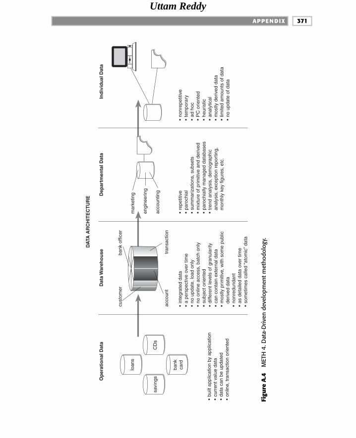
APPENDIX 371

Ind

ivid

ual

Dat

a

•no

nrep

etiti

ve•

tem

pora

ry•

ad h

oc•

PC

orie

nted

•he

uris

tic•

anal

ytic

al•

mos

tly d

eriv

ed d

ata

•lim

ited

amou

nts

of d

ata

•no

upd

ate

of d

ata

Dep

artm

enta

l Dat

a

•re

petit

ive

•pa

roch

ial

•su

mm

ariz

atio

ns, s

ubse

ts•

mix

ture

of p

rimiti

ve a

nd d

eriv

ed•

paro

chia

lly m

anag

ed d

atab

ases

•tr

end

anal

ysis

, dem

ogra

phic

anal

ysis

, exc

eptio

n re

port

ing,

mon

thly

key

figu

res,

etc

.

mar

ketin

g

engi

neer

ing

acco

untin

g

Dat

a W

areh

ou

se

•in

tegr

ated

dat

a•

a pe

rspe

ctiv

e ov

er ti

me

•no

upd

ate,

load

onl

y•

no o

nlin

e ac

cess

, bat

ch o

nly

•su

bjec

t orie

nted

•di

ffere

nt le

vels

of g

ranu

larit

y•

can

cont

ain

exte

rnal

dat

a•

mos

tly p

rimiti

ve, w

ith s

ome

publ

icde

rived

dat

a•

nonr

edun

dant

•as

det

aile

d da

ta o

ver

time

•so

met

imes

cal

led

“ato

mic

” dat

a

bank

offi

cer

tran

sact

ion

acco

unt

cust

omer

Op

erat

ion

al D

ata

•bu

ilt a

pplic

atio

n by

app

licat

ion

•cu

rren

t val

ue d

ata

•da

ta c

an b

e up

date

d•

onlin

e, tr

ansa

ctio

n or

ient

ed

savi

ngs

CD

s

loan

s

bank

card

DA

TA A

RC

HIT

EC

TU

RE

Figu

re A

.4M

ETH

4. D

ata-

Driv

en d

evel

opm

ent m

etho

dolo

gy.

Uttam Reddy

A P P E N D I X372

Dat

a W

areh

ou

se

•in

tegr

ated

dat

a•

a pe

rspe

ctiv

e ov

er ti

me

•no

upd

ate,

load

onl

y•

no o

nlin

e ac

cess

, bat

ch o

nly

•su

bjec

t orie

nted

•di

ffere

nt le

vels

of g

ranu

larit

y•

can

cont

ain

exte

rnal

dat

a•

mos

tly p

rimiti

ve, w

ith s

ome

publ

icde

rived

dat

a•

nonr

edun

dant

•as

det

aile

d da

ta o

ver

time

•so

met

imes

cal

led

“ato

mic

” dat

a

bank

offi

cer

tran

sact

ion

acco

unt

cust

omer

Op

erat

ion

al D

ata

•bu

ilt a

pplic

atio

n by

app

licat

ion

•cu

rren

t val

ue d

ata

•da

ta c

an b

e up

date

d•

onlin

e, tr

ansa

ctio

n or

ient

ed

savi

ngs

CD

s

loan

s

bank

card

data

mod

el

cont

ext l

evel

pseu

doco

dP

DIS

cont

ext l

evel

data

sto

re

defin

ition

desi

gn

revi

ew

requ

irem

ents

form

aliz

atio

n

cont

ext l

evel

1-n

DF

D (

for

each

com

pone

nt)

algo

rithm

ic s

pecs

;

perf

orm

ance

ana

lysi

s

codi

ng

wal

kthr

ough

com

pila

tion

test

ing

impl

emen

tatio

n

P1 P3

P4

P5

P7

P8 P9

P10 P11

PR

EQ

1

M3

D2

D3

JA1

P2

ER

DD

1hi

gh le

vel

revi

ew

GA

1

phys

ical

data

base

desi

gn

D4

pseu

doco

deP

6

GA

2

Mm

ainl

ine

PR

EQ

prer

equi

site

Dda

ta a

naly

sis

Ppr

oces

s an

alys

is

GA

gene

ral a

ctiv

ity

JAjo

int a

ctiv

ity

ST

stre

ss te

st

CA

capa

city

ana

lysi

s

f o r e a c h p r o c e s s

f o r e a c h s u b j e c t

M4inte

rvie

ws

data

gat

herin

g

JAD

ses

sion

s

stra

tegi

c pl

an

exis

ting

syst

ems

M1

M2

use

exis

ting

code

, dat

a

capa

city

anal

ysis

CA

stre

ss te

stS

T

tech

nica

l

envi

ronm

ent

esta

blis

hed

sizi

ng,

phas

ing

cont

ext l

evel

0

func

tiona

l

deco

mpo

sitio

n

perf

orm

ance

anal

ysis

DS

S5

subj

ect

area

DS

S7

sour

cesy

stem

anal

ysis

DS

S8

spec

s

DS

S9

prog

ram

min

g

DS

S10

popu

latio

nda

ta m

odel

anal

ysis

DS

S1

brea

dbox

anal

ysis

DS

S2

data

war

ehou

seda

taba

se d

esig

n

DS

S6

tech

nica

las

sess

men

t

DS

S3

tech

nica

len

viro

nmen

tpr

epar

atio

n

DS

S4

for

each

sub

ject

Figu

re A

.5M

ETH

5.

Uttam Reddy

APPENDIX 373

Deliverables

The steps of the data-driven development methodology include a deliverable. Intruth, some steps contribute to a deliverable with other steps. For the mostpart, however, each step of the methodology has its own unique deliverable.

The deliverables of the process analysis component of the development ofoperational systems are shown by Figure A.6.

Figure A.6 shows that the deliverable for the interview and data-gatheringprocess is a raw set of systems requirements. The analysis to determine whatcode/data can be reused and the step for sizing/phasing the raw requirementscontribute a deliverable describing the phases of development.

The activity of requirements formalization produces (not surprisingly) a formalset of system specifications. The result of the functional decomposition activi-ties is the deliverable of a complete functional decomposition.

The deliverable for the dfd definition is a set of dfds that describe the functionsthat have been decomposed. In general, the dfds represent the primitive level ofdecomposition.

The activity of coding produces the deliverable of programs. And finally, theactivity of implementation produces a completed system.

The deliverables for data analysis for operational systems are shown in FigureA.7.

The same deliverables discussed earlier are produced by the interview and datagathering process, the sizing and phasing activity, and the definition of formalrequirements.

The deliverable of the ERD activity is the identification of the major subjectareas and their relationship to each other. The deliverable of the dis activity isthe fully attributed and normalized description of each subject area. The finaldeliverable of physical database design is the actual table or database design,ready to be defined to the database management system(s).

The deliverables of the data warehouse development effort are shown in FigureA.8, where the result of the breadbox analysis is the granularity and volumeanalysis. The deliverable associated with data warehouse database design isthe physical design of data warehouse tables. The deliverable associated withtechnical environment preparation is the establishment of the technical envi-ronment in which the data warehouse will exist. Note that this environmentmay or may not be the same environment in which operational systems exist.

Uttam Reddy

A P P E N D I X374

P4DFD (for each component)

P5algorithmic specs;performance analysis

P6pseudocode

P7coding

P8walkthrough

P9compilation

P10testing

P11implementation

M1• interviews• data gathering• JAD sessions• strategic plan• existing systems

M2use existing code, data

M3sizing, phasing

M4requirements formalization

P1functional decomposition

P2context level 0

P3context level 1-n

raw systemrequirements

phases ofdevelopment

formal requirements

complete functionaldecomposition

DFDs

programs

completed system

Figure A.6 METH 6. Deliverables throughout the development life cycle.

Uttam Reddy

APPENDIX 375

On a repetitive basis, the deliverables of data warehouse population activitiesare represented by Figure A.9, which shows that the deliverable for subjectarea analysis-each time the data warehouse is to be populated-is the selectionof a subject (or possibly a subset of a subject) for population.

The deliverable for source system analysis is the identification of the system ofrecord for the subject area being considered. The deliverable for the program-

D4physical database design

M1• interviews• data gathering• JAD sessions• strategic plan• existing systems

M2use existing code, data

M3sizing, phasing

M4requirements formalization

D1ERD

D2DIS

D3performance analysis



formal requirements

midlevel detailed datamodel

major subject areas

tables, databasesphysically designed

Figure A.7 METH 7. Deliverables for operational data analysis.

Uttam Reddy

A P P E N D I X376

ming phase is the programs that will extract, integrate, and change data fromcurrent value to time variant.

breadbox analysis

DSS2

granularity analysis

technical environmentpreparation

DSS4

DSS technicalenvironment readyfor loading

data warehousedatabase design

physical databasedesign

DSS6

Figure A.8 METH 8. Preliminary data warehouse deliverables.

subjectarea

DSS5


DSS7

specs

DSS8

programming

DSS9

population

DSS10

whichsubjectarea tobuild

identification ofthe system ofrecord

extract,integration, timebasis, programtransformation

usable datawarehouse

Figure A.9 METH 9. Deliverables from the steps of data warehouse development.

Uttam Reddy

APPENDIX 377

The final deliverable in the population of the data warehouse is the actual pop-ulation of the warehouse. It is noted that the population of data into the ware-house is an ongoing activity.

Deliverables for the heuristic levels of processing are not as easy to define asthey are for the operational and data warehouse levels of development. Theheuristic nature of the analytical processing in this phase is much more infor-mal. However, Figure A.10 shows some of the deliverables associated withheuristic processing based on the data warehouse.

Figure A.10 shows that data pulled from the warehouse is the result of theextraction program. The deliverable of the subsequent analysis step is furtheranalysis based on data already refined. The deliverable of the final analysis ofdata is the satisfaction (and understanding) of requirements.

A Linear Flow of Deliverables

Except for heuristic processing, a linear flow of deliverables is to be expected.Figure A.11 shows a sample of deliverables that would result from the execu-tion of the process analysis component of the data-driven developmentmethodology.

It is true that within reason there is a linear flow of deliverables; however, thelinear flow shown glosses over two important aspects:

determinedata needed

IND1

program toextract data

IND2

analyze data

IND4

fulfilledrequirements

data pulledfrom thewarehouse

program tomerge, analyze,combine withother data

analysis withother relevantdata

IND3

Figure A.10 METH 10. Deliverables for the heuristic level of processing.

Uttam Reddy

A P P E N D I X378

■■ The deliverables are usually produced in an iterative fashion.

■■ There are multiple deliverables at any given level. In other words, deliver-ables at any one level have the capability of spawning multiple deliverablesat the next lower level, as shown by Figure A.12.

Figure A.12 shows that a single requirements definition results in three devel-opment phases. Each development phase goes through formal requirementsdefinition and into decomposition. From the decomposition, multiple activitiesare identified, each of which has a dfd created for it. In turn, each dfd createsone or more programs. Ultimately, the programs form the backbone of the com-pleted system.

completed system



formalrequirements


DFDs

programs

Figure A.11 METH 11. A linear flow of deliverables for operational process analysis.

TEAMFLY

Team-Fly®

Uttam Reddy

APPENDIX 379

Estimating Resources Required forDevelopment

Looking at the diagram shown in Figure A.12, it becomes apparent that once thespecifics of exactly how many deliverables are being spawned are designed,then an estimation of how many resources the development process will takecan be rationally done.

Figure A.13 shows a simple technique, in which each level of deliverables firstis defined so that the total number of deliverables is known. Then the time



formalrequirements


DFDs

programs

completed system

Figure A.12 METH 12. Deliverables usually spawn multiple deliverables at a lower level.

Uttam Reddy

A P P E N D I X380

required for the building of each deliverable is multiplied by each deliverable,yielding an estimate of the employee resources required.

SDLC/CLDS

Earlier discussions alluded to the fact that operational systems are built underone system development life cycle, and DSS systems are built under anothersystem development life cycle. Figure A.14 shows the development life cycleassociated with operational systems, where requirements are at the startingpoint. The next activities include analysis, design, programming, testing, inte-gration, implementation, and maintenance.

The system development life cycle associated with DSS systems is shown byFigure A.15, where DSS processing begins with data. Once data for analysis issecured (usually by using the data warehouse), programming, analysis, and soforth continue. The development life cycle for DSS data ends with an under-standing of the requirements.

no del × del = _______

no del × del = _______

no del × del = _______

no del × del = _______

no del × del = _______

no del × del = _______

Figure A.13 METH 13. stimating system development time.

Uttam Reddy

APPENDIX 381

context level

pseudocodP

DIScontext level

data store

definition

design

review

requirements

formalization

context level 1-n

DFD (for each component)

algorithmic specs;

performance analysis

coding

walkthrough

compilation

testing

implementation

P1

P3

P4

P5

P7

P8

P9

P10

P11

PREQ1

M3

D2

D3

JA1

P2

ERDD1 high level

review

GA1

physical

database

design

D4

pseudocodeP6

GA2

M mainline

PREQ prerequisite

D data analysis

P process analysis

GA general activity

JA joint activity

ST stress test

CA capacity analysis

f

o

r

e

a

c

h

p

r

o

c

e

s

s

f

o

r

e

a

c

h

s

u

b

j

e

c

t

M4

interviews

data gathering

JAD sessions

strategic plan

existing systems

M1

M2 use existing

code, data

capacity

analysis

CA

stress testST

technical

environment

established

sizing,

phasing

context level 0

functional

decomposition

performance

analysis

requirements

analysis

design

programming

testing

integration

implementation

maintenance

the classical system development lifecycle

Figure A.14 METH 14.

Uttam Reddy

APPENDIX 383

The data dictionary plays a central role in operational processing in the activi-ties of ERD development and documentation, DIS development, physical data-base design, and coding. The data dictionary plays a heavy role in data modelanalysis, subject area selection, source system selection (system of recordidentification), and programming in the world of data warehouse development.

What about Existing Systems?

In very few cases is development done freshly with no backlog of existing sys-tems. Existing systems certainly present no problem to the DSS component ofthe data-driven development methodology. Finding the system of record inexisting systems to serve as a basis for warehouse data is a normal event.

datamodel

analysis

subjectarea


specs

programming

ERD

DIS

performanceanalysis

physicaldatabase

design

pseudocode

coding

data dictionary

operationaldevelopment

the role of the data dictionaryin the development processfor data-driven development

Figure A.16 METH 16. Data warhouse development.

Uttam Reddy

A P P E N D I X384

A word needs to be said about existing systems in the operational environment.The first approach to existing operational systems is to try to build on them.When this is possible, much productivity is the result. But in many cases exist-ing operational systems cannot be built on.

The second stance is to try to modify existing operational systems. In somecases, this is a possibility; in most cases, it is not.

The third stance is to do a wholesale replacement and enhancement of existingoperational systems. In this case, the existing operational system serves as abasis for gathering requirements, and no more.

A variant of a wholesale replacement is the conversion of some or all of anexisting operational system. This approach works on a limited basis, where theexisting system is small and simple. The larger and more complex the existingoperational system, the less likelihood that the system can be converted.

Uttam Reddy

Installing Custom Controls 385G LO S S A RY

access the operation of seeking, reading, or writing data on a storage unit.

access method a technique used to transfer a physical record from or to amass storage device.

access pattern the general sequence in which the data structure is accessed(for example, from tuple to tuple, from record to record, from segment to seg-ment, etc.).

accuracy a qualitative assessment of freedom from error or a quantitativemeasure of the magnitude of error, expressed as a function of relative error.

ad hoc processing one-time-only, casual access and manipulation of data onparameters never before used, usually done in a heuristic, iterative manner.

after image the snapshot of data placed on a log on the completion of atransaction.

agent of change a motivating force large enough not to be denied, usuallyaging of systems, changes in technology, radical changes in requirements, etc.

algorithm a set of statements organized to solve a problem in a finite numberof steps.

alternate storage storage other than disk-based storage used to hold bulkamounts of relatively inactive storage.

385

Uttam Reddy

analytical processing using the computer to produce an analysis for man-agement decision, usually involving trend analysis, drill-down analysis, demo-graphic analysis, profiling, etc.

application a group of algorithms and data interlinked to support an organi-zational requirement.

application database a collection of data organized to support a specificapplication.

archival database a collection of data containing data of a historical nature.As a rule, archival data cannot be updated. Each unit of archival data is relevantto a moment in time, now passed.

artifact a design technique used to represent referential integrity in the DSSenvironment.

atomic (1) data stored in a data warehouse; (2) the lowest level of processanalysis.

atomic database a database made up of primarily atomic data; a data ware-house; a DSS foundation database.

atomic-level data data with the lowest level of granularity. Atomic-level datasits in a data warehouse and is time-variant (i.e., accurate as of some momentin time now passed).

attribute a property that can assume values for entities or relationships.Entities can be assigned several attributes (for example, a tuple in a relation-ship consists of values). Some systems also allow relationships to have attrib-utes as well.

audit trail data that is available to trace activity, usually update activity.

backup a file serving as a basis for the activity of backing up a database. Usu-ally a snapshot of a database as of some previous moment in time.

batch computer environment in which programs (usually long-running,sequentially oriented) access data exclusively, and user interaction is notallowed while the activity is occurring.

batch environment a sequentially dominated mode of processing; in batch,input is collected and stored for future, later processing. Once collected, thebatch input is transacted sequentially against one or more databases.

before image a snapshot of a record prior to update, usually placed on anactivity log.

bitmap a specialized form of an index indicating the existence or nonexis-tence of a condition for a group of blocks or records. Bitmaps are expensive tobuild and maintain but provide very fast comparison and access facilities.

GLOSSARY386

Uttam Reddy

blocking the combining of two or more physical records so that they arephysically located together. The result of their physical colocation is that theycan be accessed and fetched by a single execution of a machine instruction.

cache a buffer usually built and maintained at the device level. Retrievingdata out of a cache is much quicker than retrieving data out of a cylinder.

cardinality (of a relation) the number of tuples (i.e., rows) in a relation.

CASE computer-aided software engineering

checkpoint an identified snapshot of the database or a point at which thetransactions against the database have been frozen or have been quiesced.

checkpoint/restart a means of restarting a program at some point otherthan the beginning for example, when a failure or interruption has occurred. Ncheckpoints may be used at intervals throughout an application program. Ateach of those points, sufficient information is stored to permit the program tobe restored to the moment in time the checkpoint has been taken.

CLDS the facetiously named system development life cycle for analytical,DSS systems. CLDS is so named because, in fact, it is the reverse of the classi-cal systems development life cycle SDLC.

clickstream data data generated in the Web environment that tracks theactivity of the users of the Web site.

column a vertical table in which values are selected from the same domain. Arow is made up of one or more columns.

Common Business Oriented Language (COBOL) a computer languagefor the business world. A very common language.

commonality of data similar or identical data that occurs in different appli-cations or systems. The recognition and management of commonality of data isone of the foundations of conceptual and physical database design.

compaction a technique for reducing the number of bits required to repre-sent data without losing the content of the data. With compaction, repetitivedata are represented very concisely.

condensation the process of reducing the volume of data managed withoutreducing the logical consistency of the data. Condensation is essentially differ-ent from compaction.

contention the condition that occurs when two or more programs try toaccess the same data at the same time.

continuous time span data data organized so that a continuous definitionof data over a span of time is represented by one or more records.

GLOSSARY 387

Uttam Reddy

corporate information factory (CIF) the framework that exists that sur-rounds the data warehouse; typically contains an ODS, a data warehouse, datamarts, DSS applications, exploration warehouses, data mining warehouses,alternate storage, and so forth

CPU central processing unit.

CPU-bound the state of processing in which the computer can produce nomore output because the CPU portion of the processor is being used at 100 per-cent capacity. When the computer is CPU-bound, typically the memory andstorage processing units are less than 100 percent utilized. With modern DBMS,it is much more likely that the computer is I/O-bound, rather than CPU-bound.

CRM customer relationship management, a popular DSS applicationdesigned to streamline customer/corporate relationships.

cross-media storage manager software whose purpose is to move data toand from disk storage and alternate storage.

current value data data whose accuracy is valid as of the moment of execu-tion, as opposed to time-variant data.

DASD see direct access storage device.

data a recording of facts, concepts, or instructions on a storage medium forcommunication, retrieval, and processing by automatic means and presenta-tion as information that is understandable by human beings.

data administrator (DA) the individual or organization responsible for thespecification, acquisition, and maintenance of data management software andthe design, validation, and security of files or databases. The data model andthe data dictionary are classically the charge of the DA.

database a collection of interrelated data stored (often with controlled, lim-ited redundancy) according to a schema. A database can serve single or multi-ple applications.

database administrator (DBA) the organizational function charged withthe day-to-day monitoring and care of the databases. The DBA function is moreclosely associated with physical database design than the DA is.

database key a unique value that exists for each record in a database. Thevalue is often indexed, although it can be randomized or hashed.

database management system (DBMS) a computer-based software sys-tem used to establish and manage data.

data-driven development the approach to development that centersaround identifying the commonality of data through a data model and buildingprograms that have a broader scope than the immediate application. Data-driven development differs from classical application-oriented development.

GLOSSARY388

Uttam Reddy

data element (1) an attribute of an entity; (2) a uniquely named and well-defined category of data that consists of data items and that is included in arecord of an activity.

data item set (dis) a grouping of data items, each of which directly relatesto the key of the grouping of data in which the data items reside. The data itemset is found in the midlevel model.

data mart a departmentalized structure of data feeding from the datawarehouse where data is denormalized based on the department’s need forinformation.

data mining the process of analyzing large amounts of data in search of pre-viously undiscovered business patterns.

data model (1) the logical data structures, including operations and con-straints provided by a DBMS for effective database processing; (2) the systemused for the representation of data (for example, the ERD or relational model).

data structure a logical relationship among data elements that is designedto support specific data manipulation functions (trees, lists, and tables).

data warehouse a collection of integrated, subject-oriented databasesdesigned to support the DSS function, where each unit of data is relevant tosome moment in time. The data warehouse contains atomic data and lightlysummarized data.

decision support system (DSS) a system used to support managerial deci-sions. Usually DSS involves the analysis of many units of data in a heuristicfashion. As a rule, DSS processing does not involve the update of data.

decompaction the opposite of compaction; once data is stored in a com-pacted form, it must be decompacted to be used.

denormalization the technique of placing normalized data in a physical loca-tion that optimizes the performance of the system.

derived data data whose existence depends on two or more occurrences ofa major subject of the enterprise.

derived data element a data element that is not necessarily stored but thatcan be generated when needed (age, current date, date of birth).

design review the quality assurance process in which all aspects of a systemare reviewed publicly prior to the striking of code.

dimension table the place where extraneous data that relates to a fact tableis placed in a multidimensional table.

direct access retrieval or storage of data by reference to its location on a vol-ume. The access mechanism goes directly to the data in question, as is generallyrequired with online use of data. Also called random access or hashed access.

GLOSSARY 389

TEAMFLY

Team-Fly®

Uttam Reddy

direct access storage device (DASD) a data storage unit on which datacan be accessed directly without having to progress through a serial file such asa magnetic tape file. A disk unit is a direct access storage device.

dormant data data that is very infrequently used.

download the stripping of data from one database to another based on thecontent of data found in the first database.

drill-down analysis the type of analysis where examination of a summarynumber leads to the exploration of the components of the sum.

DSS application an application whose foundation of data is the data ware-house.

dual database the practice of separating high-performance, transaction-oriented data from decision support data.

dual database management systems the practice of using multiple data-base management systems to control different aspects of the database environ-ment.

dumb terminal a device used to interact directly with the end user where allprocessing is done on a remote computer. A dumb terminal acts as a device thatgathers data and displays data only.

estetbusiness commerce conducted based on Web interactions.

encoding a shortening or abbreviation of the physical representation of adata value (e.g., male � “M,” female � “F”).

enterprise resource planning (ERP) application software for processingtransactions.

entity a person, place, or thing of interest to the data modeler at the highestlevel of abstraction.

entity-relationship diagram (ERD) a high-level data model; the schematicshowing all the entities within the scope of integration and the direct relation-ship between those entities.

event a signal that an activity of significance has occurred. An event is notedby the information system.

Executive Information Systems (EIS) systems designed for the top exec-utive, featuring drill-down analysis and trend analysis.

extract/load/transformation (ETL) the process of taking legacy applica-tion data and integrating it into the data warehouse.

external data (1) data originating from other than the operational systemsof a corporation; (2) data residing outside the central processing complex.

GLOSSARY390

Uttam Reddy

exploration warehouse a structure specifically designed for statistical pro-cessing that searches for business patterns.

extract the process of selecting data from one environment and transportingit to another environment.

fact table the center of a star join table where data that has many occur-rences will be located.

flat file a collection of records containing no data aggregates, nestedrepeated data items, or groups of data items.

foreign key an attribute that is not a primary key in a relational system butwhose values are the values of the primary key of another relation.

fourth-generation language language or technology designed to allow theend user unfettered access to data.

functional decomposition the division of operations into hierarchical func-tions (activities) that form the basis for procedures.

global data warehouse a warehouse suited to the needs of headquarters ofa large corporation.

granularity the level of detail contained in a unit of data. The more detailthere is, the lower the level of granularity. The less detail there is, the higher thelevel of granularity.

granularity manager the software or processes that edit and filter Web dataas it flows into the data warehouse. The data that flows into the data warehouseenvironment from the Web environment is usually clickstream data that isstored in a Web log.

heuristic the mode of analysis in which the next step is determined by theresults of the current step of analysis. Used for decision support processing.

image copy a procedure in which a database is physically copied to anothermedium for the purposes of backup.

index the portion of the storage structure maintained to provide efficientaccess to a record when its index key item is known.

information data that human beings assimilate and evaluate to solve a prob-lem or make a decision.

integrity the property of a database that ensures that the data contained inthe database is as accurate and consistent as possible.

interactive a mode of processing that combines some of the characteristicsof online transaction processing and batch processing. In interactive process-ing, the end user interacts with data over which he or she has exclusive control.

GLOSSARY 391

Uttam Reddy

master file a file that holds the system of record for a given set of data (usu-ally bound by an application).

metadata (1) data about data; (2) the description of the structure, content,keys, indexes, etc., of data.

microprocessor a small processor serving the needs of a single user.

migration the process by which frequently used items of data are moved tomore readily accessible areas of storage and infrequently used items of data aremoved to less readily accessible areas of storage.

million instructions per second (mips) the standard measurement ofprocessor speed for minicomputers and mainframe computers.

multidimensional processing data mart processing based on a star joinstructuring of data.

near line storage data that is not stored on disk but is never the less stillaccessible; used to hold very large amounts of relatively inactive data.

online analytical processing (OLAP) departmental processing for thedata mart environment.

online storage storage devices and storage media where data can beaccessed in a direct fashion.

operational data data used to support the daily processing a company does.

operational data store (ODS) a hybrid structure designed to support bothoperational transaction processing and analytical processing.

operations the department charged with the running of the computer.

optical disk a storage medium using lasers as opposed to magnetic devices.Optical disk is typically write only, is much less expensive per byte than mag-netic storage, and is highly reliable.

overflow (1) the condition in which a record or a segment cannot be storedin its home address because the address is already occupied. In this case, thedata is placed in another location referred to as overflow; (2) the area of DASDwhere data is sent when the overflow condition is triggered.

ownership the responsibility for updating operational data.

page (1) a basic unit of data on DASD; (2) a basic unit of storage in mainmemory.

parameter an elementary data value used as a criterion for qualification, usu-ally of data searches or in the control of modules.

GLOSSARY 393

Uttam Reddy

repeating groups a collection of data that can occur several times within agiven record occurrence.

rolling summary a form of storing archival data where the most recent datahas the most details stored, and data that is older has fewer details stored.

scope of integration the formal definition of the boundaries of the systembeing modeled.

SDLC system development life cycle; the classical operational system devel-opment life cycle that typically includes requirements gathering, analysis,design, programming, testing, integration, and implementation.

sequential file a file in which records are ordered according to the values ofone or more key fields. The records can be processed in this sequence startingfrom the first record in the file, continuing to the last record in the file.

serial file a sequential file in which the records are physically adjacent, insequential order.

set-at-a-time processing access of data by groups, each member of whichsatisfies a selection criterion.

snapshot a database dump or the archiving of data out of a database as ofsome moment in time.

snowflake structure the result of joining two or more star joins.

spiral development iterative development, as opposed to waterfall develop-ment.

solutions database the component of a DSS environment where the resultsof previous decisions are stored. Solutions databases are consulted to helpdetermine the proper course of action in a current decision-making situation.

staging area a place where data in transit is placed, usually coming from thelegacy environment prior to entering the ETL layer of processing.

star join a data structure where data is denormalized to optimize the accessof the data; the basis of multidimensional data mart design.

storage hierarchy storage units linked to form a storage subsystem, inwhich some units are fast but small and expensive, and other units are large butslower and less expensive.

subject database a database organized around a major subject of the corpo-ration. Classical subject databases are for customer, transaction, product, part,vendor.

GLOSSARY 395

Uttam Reddy

Installing Custom Controls 397R E F E R E N C E S

Articles

Adelman, Sid. “The Data Warehouse Database Explosion.” DMR (December1996). A very good discussion of why volumes of data are growing as fast asthey are in the data warehouse environment and what can be done about it.

Kalman, David. “The Doctor of DSS.” DBMS Magazine (July 1994). An inter-view with Ralph Kimball.

Geiger, Jon. “Data Element Definition.” DMR (December 1996). A good descrip-tion of the definitions required in the system of record.

––––. “What’s in a Name.” Data Management Review (June 1996). A discussionof the implications of naming structures in the data warehouse environment.

Gilbreath, Roy, M.D. “Informational Processing Architecture for OutcomesManagement.” A description of data warehouse as it applies to health careand outcomes analysis. Under review.

Gilbreath, Roy, M.D., Jill Schilp, and Robert Pickton “Towards an OutcomesManagement Informational Processing Architecture.” HealthCare Informa-

tion Management 10, No. 1 (Spring 1996). A discussion of the architectedenvironment as it relates to healthcare.

397

Uttam Reddy

––––. “Managing the Data Warehouse: The Data Content card Catalog.” DMR

(December 1996). An introduction to the notion of a data content card cata-log, that is, the stratification of data content.

––––. “Managing the Data Warehouse Environment.” Data Management

Review (February 1996). Defining who the data warehouse administrator is.

––––. “Measuring Capacity in the Data Warehouse.” Enterprise Systems Jour-

nal (August 1996). A discussion of how capacity should be measured in thedata warehouse and DSS environment.

––––. “Monitoring the Data Warehouse Environment.” Data Management

Review (January 1996). What is a data monitor for the data warehouse envi-ronment and why would you need it.

––––. “Rethinking Data Relationships for Warehouse Design.” Sybase Server 5,No. 1 (Spring 1996). A discussion of the issues data warehouse data relation-ships.

––––. “SAP and the Data Warehouse.” DMR (July/Aug 1996). A description ofwhy the data warehouse is still needed in the face of SAP.

––––. “Security in the Data Warehouse: Data Privatization.” Enterprise Systems

Journal (March 1996). Data warehouse requires a very different approach tosecurity than the traditional VIEW-based approach offered by DBMS ven-dors.

––––. “Summary Data: The New Frontier.” Data Management Review (May1996). A description of the different types of summary data, includingdynamic summary data, static summary data, lightly summarized data, andhighly summarized data.

Inmon, W.H. “User Reaction to the Data Warehouse.” DMR (December 1996). Adescription of the different user types in data warehousing.

––––. “Virtual Data Warehouse: The Snake Oil of the ‘90s.” Data Management

Review (April 1996). A discussion of the virtual data warehouse and how theconcept tries to attach itself to the legitimacy of the data warehouse.

“In the Words of Father Inmon.” MIS (February 1996) An interview with BillInmon in November of 1995 in Australia.

Jordan, Arthur. “Data Warehouse Integrity: How Long and Bumpy the Road?”Data Management Review (March 1996). A discussion of the issues of dataquality inside the data warehouse.

Lambert, Bob. “Break Old Habits to Define Data Warehousing Requirements.”Data Management Review (December 1995). A description of how the enduser should be approached to determine DSS requirements.

––––. “Data Warehousing Fundamentals: What You Need to Know to Succeed.”Data Management Review (March 1996). Several significant strategies fordata warehousing to guide you through a successful implementation.

R E F E R E N C E S 399

Uttam Reddy

Dodge, Gary, and Tim Gorman. Oracle8i Data Warehousing. New York: JohnWiley & Sons. 2000.

Dyche, Jill. The CRM Handbook. Reading, MA: Addison Wesley. 2001.

––––. E-data: Turning Data into Information with Data Warehousing. Read-ing, MA: Addison Wesley. 2000.

English, Larry. Improving Data Warehouse and Business Information Qual-

ity. New York: John Wiley & Sons. 1999.

Hackathorn, Richard. Web Farming for the Data Warehouse, San Francisco:Morgan Kaufman. 1998.

Imhoff, Claudia, Lisa Loftis, and John Geiger. Building the Customer-Centric

Enterprise. New York: John Wiley & Sons. 2001.

Inmon, W.H. Building the Data Warehouse. New York: John Wiley & Sons. 1996.

––––. Building the Data Warehouse, Second Edition. New York: John Wiley &Sons. 1996.

––––. Building the Operational Data Store, Second Edition. New York: JohnWiley & Sons. 1999.

––––. Data Architecture: The Information Paradigm. New York: QED. 1993.

––––. Third Wave Processing: Database Machines and Decision Support Sys-

tems. New York: John Wiley & Sons. 1993.

Inmon, W.H. and Richard Hackathorn. Using the Data Warehouse. New York:John Wiley & Sons. 1994.

Inmon, W.H., Jon Geiger, and John Zachman. Data Stores, Data Warehousing

and the Zachman Framework. New York: McGraw Hill. 1997.

Inmon, W.H., Katherine Glassey, and J.D. Welch. Managing the Data Ware-

house. New York: John Wiley & Sons. 1996.

Inmon, W.H., Claudia Imhoff, and Ryan Sousa. Corporate Information Factory:Third Edition. New York: John Wiley & Sons. 2000.

Inmon, W.H. and Jeff Kaplan. Information Systems Architecture: Development

in the 90s. New York: John Wiley & Sons. 1993.

Inmon, W.H. and Chuck Kelley. RDB/VMS: Developing the Data Warehouse.Boston. QED Pub Group. 1993.

Inmon, W.H., Joyce Montanari, Bob Terdeman, and Dan Meers. Data Ware-

housing for E-Business. New York: John Wiley & Sons. 2001.

Inmon, W.H. and Sue Osterfelt. Understanding Data Pattern Processing. NewYork: QED. 1993.

Inmon, W.H., Ken Rudin, Christopher Buss, and Ryan Sousa. Data Warehouse

Performance. New York: John Wiley & Sons. 1998.


Uttam Reddy

Inmon, W.H. and R.H. Terdeman. Exploration Warehousing. New York: JohnWiley & Sons. 2000.

Kachur, Richard. Data Warehouse Management Handbook. Englewood Cliffs,NJ: Prentice Hall. 2000.

Kelly, Sean. Data Warehousing: The Key to Mass Customization. New York:John Wiley & Sons. 1996.

Kimball, Ralph, and Richard Merz. The Data Webhouse Toolkit. New York: JohnWiley & Sons. 2000.

Kimball, Ralph, Laura Reeves, Margy Ross, and Warren Thornthwaite. The Data

Warehouse Lifecycle Toolkit. New York: John Wiley & Sons. 1998.

Kimball, Ralph, and Margy Ross. The Data Warehouse Toolkit: Practical Tech-

niques for Building Dimensional Data Warehouses. New York: John Wiley& Sons. 2002.

Love, Bruce. Enterprise Information Technologies. New York: John Wiley &Sons. 1993.

Marco, David. Meta Data Repository. New York: John Wiley & Sons. 2000.

Parsaye, Kamran and Marc Chignell. Intelligent Database Tools and Applica-

tions. New York: John Wiley & Sons. 1989.

Silverston, Len. The Data Model Resource Book Volume I. New York: John Wiley& Sons. 2001.

Sullivan, Dan. Document Warehousing and Text Mining. New York: John Wiley& Sons. 2001.

Swift, Ron. Accelerating Customer Relationships. Englewood Cliffs, NJ: Pren-tice Hall. 2000.

Tannenbaum, Adrienne. Metadata Solutions. Reading, MA: Addison Wesley.2002.

White Papers

Available on www.billinmon.com

“Accessing Data Warehouse Data from the Operational Environment.” Mostdata flow is from the operational environment to the data warehouse envi-ronment, but not all. This Tech Topic discusses the “backward” flow of data.

“Building the Data Mart or the Data Warehouse First?” Although the data martis a companion to the data warehouse, data mart vendors try to encouragepeople to build the data mart without building the data warehouse. This TechTopic addresses the issues relevant to this important design decision.

R E F E R E N C E S402

Uttam Reddy

“Capacity Planning for the Data Warehouse.” This Tech Topic discusses theissue of capacity planning and projection for both disk storage and proces-sor resources for the data warehouse environment.

“Changed Data Capture.” The resources required for repeatedly scanning theoperational environment for the purpose of refreshing the data warehousecan be enormous. This briefing addresses an alternative way to accomplishthe same thing.

“Charge Back in the Data Warehouse DSS Environment.” Charge back is anextremely useful way to get the end user to take responsibility for theresources that are being consumed. This Tech Topic addresses the issues ofcharge back.

“Client/Server and Data Warehouse.” Client/server processing is quite able tosupport data warehouse processing. This Tech Topic addresses the issues ofarchitecture and design.

“Creating the Data Warehouse Data Model from the Corporate Data Model.”This paper outlines the steps you need to take to create the data warehousedata model from the corporate data model.

“Data Mining: An Architecture.” Using the data warehouse is an art. This TechTopic relates the underlying architecture of the data warehouse to thesophisticated way in which the data warehouse can be used.

“Data Mining: Exploring the Data.” Once the data is gathered and organized andthe architecture for exploitation has been built, the task remains to use thedata. This Tech Topic addresses how data can be mined once the architec-ture is built.

“Data Stratification in the Data Warehouse.” How do you tell someone what isinside a 1-terabyte data warehouse? How many customers? Of what type? Ofwhat age? Living where? Buying how much per year? This Tech Topicaddresses the technique of stratifying data in order to create a library “tableof contents” that describes the actual data content inside a data warehouse.

“Data Warehouse Administration.” With DSS and data warehouses comes theneed to manage the environment. A new organizational function has arisen:data warehouse administration. This Tech Topic addresses the charter ofdata warehouse administration and other important data managementissues.

“Data Warehouse Administration in the Organization.” Once the need for datawarehouse administration is recognized, there is the question, Where shouldthe DWA function be placed in the organization? This Tech Topic addressesthe issues of the organization placement of the DWA function.

“The Data Warehouse Budget.” This Tech Topic addresses the different patternsof spending and the rate at which funds are spent. In addition, some sugges-tions for minimizing expenses are included.


Uttam Reddy

uted metadata architecture that enables metadata to be simultaneously dis-tributed and managed autonomously.

“Monitoring Data Warehouse Activity.” Activity in the data warehouse needs tobe monitored for a variety of reasons. This Tech Topic describes monitoringtechniques and considerations, as well as a description of why activity mon-itoring needs to be done

“Monitoring Data Warehouse Data.” Although activity monitoring is very impor-tant, so is the monitoring of data itself in the data warehouse. The growth ofthe data, the quality of the data, and the actual content of the data are all atstake in this issue.

“OLAP and Data Warehouse.” Lightly summarized data has always been an inte-gral part of the data warehouse architecture. Today this construct is know asOLAP or a data mart. This Tech Topic addresses the relationship of OLAPand the detailed data found in the data warehouse.

“The Operational Data Store.” The operational counterpoint of the data ware-house is the operational data store (the ODS). The ODS is defined anddescribed in detail in this tech topic.

“Operational and DSS Processing from a Single Database: Separating Fact andFiction.” An early notion was that a single database should serve as the basisfor both operational processing and DSS analytical processing. This TechTopic explores the issues and describes why a data warehouse is the appro-priate foundation for DSS informational processing

“Parallel Processing in the Data Warehouse.” The management of volumes ofdata is the first and major challenge facing the data architect. Parallel tech-nology offers the possibility of managing much data. This Tech Topic is onthe issues of parallel technology in the data warehouse environment.

“Performance in the Data Warehouse Environment.” Performance is as impor-tant in the DSS data warehouse environment as it is in the OLTP environ-ment. However, performance plays a very different role. This Tech Topic isall about performance in the DSS data warehouse environment.

“Reengineering and the Data Warehouse.” Many organizations are not aware ofthe strong and positive relationship between reengineering and the datawarehouse. This topic identifies the relationship and discusses the ramifica-tions.

“Representing Data Relationships in the Data Warehouse: Artifacts of Data.”Design issues for the building of data relationships in the data warehouse

“Security in the Data Warehouse.” Security takes on a different dimension in thedata warehouse than in other data processing environment. This Tech Topicdescribes the issues. Tech Topics are available from PRISM Solutions.


TEAMFLY

Team-Fly®

Uttam Reddy

“Service Level Agreements in the Data Warehouse Environment.” One of thecornerstones of online operations is the service level agreement. Servicelevel agreements are applicable to the data warehouse, but are implementedquite differently.

“Snapshots of Data in the Warehouse.” A description of the different types ofsnapshots and the advantages and disadvantages of each.

“Summary Data in the Data Warehouse/Operational Data Store.” Summary datahas its own set of unique considerations. There is, for example, dynamicsummary data and static summary data. Both types of summary data requirevery different treatment from the designer and the end user. This Tech Topiccreates a taxonomy for summary data and relates the different types of sum-mary data to the data warehouse and the operational data store.

“Telling the Difference Between Operational and DSS.” In every shop, the issuearises: what is operational and what is DSS. This Tech Topic tells you how totell the difference between the two environments.

“Time-Dependent Data Structures.” A discussion of the different types of datastructures and their advantages and disadvantages

“Using the Generic Data Model.” Some corporations have a data model as apoint of departure for the design of their data warehouse; others do not. Thegeneric data model jump-starts the data warehouse design and developmenteffort.

“What Is a Data Mart?” Data marts are a natural emanation from the data ware-house. This Tech Topic outlines the salient characteristics of the data mart.

“What Is a Data Warehouse?” This Tech Topic defines what a data warehouse isand what its structure looks like. This is a basic discussion appropriate toanyone investigating the world of data warehouse.

For more white papers, refer to the Web site, www.billinmon.com.

R E F E R E N C E S406

Uttam Reddy

I N D E X

407

Aaccess of data, global and

local data warehouses,216–219

administering design reviews, 324

agenda, design reviews, 323airline commission

calculation system,130–131

algorithmic differential, 8alternate storage, design

reviews, 341analysis example, EIS,

248–250analytical program, 303application-level

partitions, 58architected environment

data integration, 19levels of data, 17migration, 277

architectural changes, naturally evolving architecture, 15

archival data, 74external data, 275operational window, 75

atomic data, 254attendees, design reviews,

323–324auditing, 64, 335

Bbackflow, 337banking systems,

granularity levels, 158,162–163

buildingcosts, 68–69data warehouse

in ERP structure, 314outside ERP

structure, 315business needs, design

reviews, 326

CCDC (changed data

capture), 196–197class IV ODS, design

reviews, 339CLDS, 21clickstream data, 298–299collectiive view of data, 47compaction, 47, 175, 335completely unrelated

warehouses, 224–225complex contextual

data, 194complexity of

transformation, 118components

external data, 272snapshots, 123unstructured data, 272

compound keys, 176connectors, DIS, 96contextual data, 192–194continuous files, 61coordinating development

among distributedlocations, 227

corporate data model, 89

distributed datawarehouses, 228, 231

migration plans, 278–279corporate information

factory, 17cost justification, 65–66cost of reports, 66–68creative indexes, 108creative profiles, 108credit scoring, 133cross media storage

managers, design reviews, 341

cumulative structures, 59cyclicity of data, 115

DDASD (direct access

storage device), 4, 39data

archival, 74compaction, 175contextual, 192–193corrections, design

reviews, 334direct access, 129heterogeneity, 69homogeneity, 69indirect access, 130integration, architected

environment, 19managing large

amounts, 167–169monitoring, 170parallel storage/

management, 171profiles, 26

Uttam Reddy

data (Continued)purges, 72relationships, design

reviews, 332replication, 196storage, design reviews,

341variable length, 176

data-driven developmentmethodologies, 291, 293

data levels, architected environment, 17

data mart level, 17data marts, star joins,

138-139, 142data mining, 53data models, 88-89, 92, 102

design reviews, 326external data, 273unstructured data, 273

data to information problems, naturallyevolving architecture,12–14

data warehouse design, 81,281

data model, 89, 92design models, 87field transformation, 83format of legacy

data, 83limiting operational data

scans, 85loading

archival data, 84current data, 85ongoing data changes,

85operational data, 82–83stability analysis, 90

data warehouse level, 17data warehouses

archival data, 74auditing, 64building costs, 68–69collective view of

data, 47

compaction, 47complexity of

transformation, 118continuous files, 61cost justification, 65–66cost of reports, 66–68cumulative

structures, 59cyclicity of data, 115data mining, 53day 1-day n

phenomenon, 41DBMS types, 179–180detail levels, 239, 242DSS analysts, 19encoding data, 33exploration, 53functionality of data

movement, 118–121granularity, 43–46hardware utilization, 23history of data, 33incorrect data, 76integration, 31interfaces, 283–284light summarization

data, 50living sample

databases, 53–55meta data, 113, 189–190monitoring

environment, 25–28multiple level, 232–235multiple storage

media, 189nonvolatility, 33partitions, 55–58physical tables, 36–38reference tables, 113–114refreshing, 195–196rolling summary

data, 59simple direct file, 61snapshots, 111standards manuals, 64storage media, 39

structure, 35subject areas, 283subject orientation,

31, 36time horizon, 34time variance, 34true archival level of

data, 51volume

management, 126databases, 4day 1-day n

phenomenon, 41DBMSs (database

managementsystems), 4

changing, 181multidimensional,

182–188types, 179–180

deliberate introduction ofredundant data, 105

delta lists, 289denormalization, 104–106departmental data level, 17derived data, 15design models, 87design reviews, 321

administering, 324agenda, 323alternate storage, 341attendees, 323–324auditing, 335changing business needs,

326class IV ODS, 339compaction, 335cross media storage

managers, 341data

corrections, 334models, 326ownership, 334relationships, 332storage, 341

dormancy rates, 339

I N D E X408

Uttam Reddy

end user requirements, 325

explorationwarehouses, 339

extent of development, 325

external data issues, 336extract processing, 327flowback, 337Granularity

Manager, 340granularity of data, 331indexing data, 330loading issues, 333locating data, 337logging, 336managing data

access, 331meta data storage, 335migration plans, 326outages, 333partitioning, 338physical data

organization, 329processing capacity

requirements, 332processing charges, 338processing volume, 331public summary

data, 334purge criteria, 331recovery times, 333reference tables, 335repetitive

processing, 337restructuring, 329SDLC, 322SLAs, 330software interfaces, 329sparse indexes, 338subject area midlevel

models, 340system of record, 327temporary indexes, 338time lag issues, 336updates, 336

volume of data, 328when to perform, 322

designing data warehouse, 81, 281

field transformation, 83format of legacy

data, 83limiting operational data

scans, 85loading

archival data, 84current data, 85ongoing data changes,

85operational data,

82–83, 86detail levels, 239, 242detailed data, EIS, 261developing distributed data

warehouses, 225–227development, 222–224development life cycle, 21direct data access, 129DIS (Data Item Set), 92–94

connectors, 96physical tables, 98primary grouping of

data, 95secondary grouping of

data, 96type-of data, 96–97

distributed data warehouses, 201–202

corporate data model,228, 231

developing, 225-227meta data, 232

dormancy rates, design reviews, 339

drill down analysis, EIS,251-253

DSS (decision support system), 2

analysts, 19monitoring system, 28

reports, 74response time, 27

dual levels of granularity, 49

Eebusiness, 307efficient index usage, 175EIS (executive information

systems), 19, 247analysis example,

248–250atomic data, 254detailed data, 261drill down analysis,

251–253event mapping, 258–260retrieving data, 256–257summary data, 262typical uses, 248

encoding data, 33end user requirements,

design reviews, 325ERD (Entity Relationship

Diagram), 92–93ERP (Enterprise Resource

Planning), 311–312building data

warehouses, 314–315corporate data

warehouse, 318–319operational

applications, 312–313ETL (extract/transform/

load), 122events

mapping, EIS, 258–260triggering snapshots, 122

exploration, 53exploration

warehouses, 339extent of development,

design reviews, 325external contextual

data, 194

INDEX 409

Uttam Reddy

external data, 265–267archiving, 275comparing to internal

data, 275components, 272data models, 273frequency of

availability, 268meta data, 269–270storage, 271

extract processing, designreviews, 327

extract program, 5

Ffast restore, 178feedback loops, 156, 286field transformation, data

warehouse design, 83flowback, 337format of legacy data, data

warehouse design, 83

frequency of availability,external data, 268

functionality of datamovement, 118–121

Gglobal data, intersection

with local data, 211–213global data warehouses,

202–209data access, 216–219redundancy with local

data, 214–215granularity, 43–46, 147

data access, 331data overflow, 151determining levels, 155

banking systems, 158,162–163

dual levels, 49feedback loops, 156levels, 47overflow storage,

151–154

planning process, 149raw estimates, 148–149

Granularity Manager, 298,306

clickstream data, 299design reviews, 340

Hhardware utilization, 22–23heterogenous data, 69historical data, 303history of data, 33homogeneous data, 69

Iimpact analysis, 289incorrect data, 76independently evolving

distributed data warehouses, 221

indexes, 170design reviews, 330efficient usage, 175processing, 178

indirect data access, 130indirect use of data, 136individual data level, 18information

processing, 1–5integration, 31interfaces, 170–171, 283–284Internet, 297

clickstream data, 298ebusiness, 307moving data to

warehouse, 307ODS, 300overflow storage, 306

interpretive data, 303iterative development, 102

Llanguage interfaces,

173–174levels

data, architectedenvironment, 17

detail, 239, 242granularity, 155

banking systems, 158,162–163

light summarization data, 50

limiting operational datascans, data warehousedesign, 85

living sample databases, 53–55

loadingarchival data, data

warehouse design, 84

current data, datawarehouse design,85

issues, design reviews, 333

ongoing data changes,data warehouse design, 85

local data, intersection withglobal data, 211–213

local data warehouses,202–205

data access, 216–219redundancy with global

data, 214–215locating data, design

reviews, 337lock management, 176logging, design

reviews, 336

Mmanaging

contextual data, 194data access, design

reviews, 331large data amounts,

167–169locks, 176meta data, 171–172

I N D E X410

Uttam Reddy

multiple media types, 169

volume, 126master files, 2media, managing multiple

types, 169meta data, 113, 189–190

distributed data warehouses, 232

external data, 269–270managing, 171–172storage, design

reviews, 335methodologies of

migration, 289–290data driven, 291–293spiral approach, 292

migration, 289–290plans, 278–279, 326to architected

environment, 277MIS (management

information systems), 4monitoring

data, 170data warehouse

environment, 25–28multidimensional DBMS,

17, 182–188multiple-level data

warehouses, 232–235,238

multiple profile records, 127

multiple storage media, 189

multiple technologyinterfaces, 170–171

Nnaturally evolving

architecture, 6changing architecture, 15inability to move from

data to information,12–14

lack of data credibility,6–8

productivity problems,9–11

near line storage, 269nonvolatility, 33normalization, 104–106

OODS (operational data

store), 144, 300–301OLTP (online transaction

processing), 4operational applications,

ERP, 312–313operational data, 16

data warehouse design,82–83

level, 17operational

development, 294operational

environment, 128operational reporting, 74operational system

changes, 287operational window, 74–75outages, design

reviews, 333overflow storage,

151–154, 306ownership of data, 334

Pparallel storage/

management of data,171

partitions, 55–58, 338PCs, 4physical data model, 99physical data

organization, 329physical model, 92physical tables, 36–38, 98planning process,

determininggranularity, 149

primary grouping of data,DIS, 95

primitive data, 15process model, 88processing

capacity requirements,332

charges, 338indexes only, 178volume, 331

productivity problems,naturally evolving architecture, 9, 11

profile data, 303profile records, 124, 127public summary data, 334purge criteria, 331purging data, 72

Qquick restore, 178

Rraw estimates,

determininggranularity, 148–149

recovery times, design reviews, 333

redundancy of data, globaland local datawarehouses, 214–215

redundant data, masterfiles, 2

reengineering, 23–24reference tables, 113–114,

335referential integrity, 109refreshing data

warehouses, 195–196repetitive processing, 337reports

costs, 66–68DSS, 74operational, 74secondary, 274

resource estimates, 289

INDEX 411

Uttam Reddy

response time, DSS, 27restructuring, design

reviews, 329Retail personalization

system, 132–133Retrieving data, EIS,

256–257ROI (return on

investment), 65rolling summary data, 59

Sscheduling design

reviews, 322scope of integration, 92–93SDLC (systems

development life cycle),21, 294, 322

secondary grouping ofdata, DIS, 96

secondary reports, 274simple contextual

data, 193simple direct file, 61SLAs (service-level

agreements), 330snapshots, 111

components, 123profile records, 124reference tables, 114triggering, 122

software interfaces, 329sparse indexes, 338spider web, 235

spiral developmentmethodologies, 292

stability analysis, 90, 282standards manuals, 64star joins, data marts,

137–139storage

external data, 271media, 39unstructured data, 271

stores of unstructured data,269

strategic issues, 287structure of data

warehouse, 35structures, cumulative, 59subject area midlevel

models, 340subject areas, 283–284subject orientation, 31, 36summary data, EIS, 262support options for

Internet, 309system of record, 280, 327

Ttechnologically

distributed data warehouses, 220–221

temporary indexes, 338testing environment, 198time horizon, 34time lag issues, 336time variance, 34transaction data, 302

triggering snapshots, 122true archival level of

data, 51type-of data, DIS, 96–97typical uses of EIS, 248

Uundisciplined external data,

268unpredictability of

external data, 268unstructured data, 265–267

components, 272data models, 273frequency of

availability, 268storage, 271

updates, design reviews, 336

Vvariable-length data, 176volume management, 126volume of data, design

reviews, 328

WWeb, 297

ebusiness, 307moving data to

warehouse, 307ODS, 300overflow storage, 306

wrinkle of time, 115

I N D E X412

Uttam Reddy

Documents

Uttam Reddy - dbmanagement.infodbmanagement.info/Books/MIX/W.H._Inmon_Building_the_Data_Wareh… · Exploration and Data Mining 53 Living Sample Database 53 Partitioning as a Design