USING THE CHAINS OF RECURRENCES ALGEBRA FOR DATA

DEPENDENCE TESTING AND INDUCTION VARIABLE

SUBSTITUTION

Name: Johnnie L. BirchDepartment: Department of Computer ScienceMajor Professor: Robert A. Van EngelenDegree: Master of ScienceTerm Degree Awarded: Fall, 2002

Optimization techniques found in today’s restructuring compilers for both

single-processor and parallel architectures are often limited by ordering relationships

between instructions that are determined during dependence analysis. Unfortunately,

the conservative nature of these algorithms combined with an inability to effectively

analyze complicated loop nestings, result in missed opportunities for identification of

loop independences. This thesis examines the use of chains of recurrences (CRs)

as a basis for performing induction expression recognition and loop dependence

analysis. Specifically, we develop efficient algorithms for generalized induction

variable substitution and non-linear dependence testing, which rely on analysis of

induction variables that satisfy linear, polynomial, and geometric recurrences.

THE FLORIDA STATE UNIVERSITY

COLLEGE OF ARTS AND SCIENCES

USING THE CHAINS OF RECURRENCES ALGEBRA FOR DATA

DEPENDENCE TESTING AND INDUCTION VARIABLE

SUBSTITUTION

By

JOHNNIE L. BIRCH

A thesis submitted to theDepartment of Computer Science

in partial fulfillment of therequirements for the degree of

Master of Science

Degree Awarded:Fall Semester, 2002

The members of the Committee approve the thesis of Johnnie L. Birch defended

on November 22 2002.

Robert A. Van EngelenProfessor Directing Thesis

Kyle GallivanCommittee Member

David WhalleyCommittee Member

Approved:

Sudhir Aggarwal, ChairDepartment of Computer Science

ACKNOWLEDGEMENTS

I would like to thank Dr. Robert A. Van Engelen, Dr. Kyle Gallivan, Dr. David

Whalley, Dr. Paul Ruscher, and Dr. Patricia Stith.

iii

TABLE OF CONTENTS

List of Tables . . . . . . . . . . . . . . . . . . . . . . . . . . . . . . . . . . . . . . . . . . . . . . . . . vi

List of Figures . . . . . . . . . . . . . . . . . . . . . . . . . . . . . . . . . . . . . . . . . . . . . . . . vii

Abstract . . . . . . . . . . . . . . . . . . . . . . . . . . . . . . . . . . . . . . . . . . . . . . . . . . . . . . ix

1. INTRODUCTION . . . . . . . . . . . . . . . . . . . . . . . . . . . . . . . . . . . . . . . . . 1

1.1 Program Optimization . . . . . . . . . . . . . . . . . . . . . . . . . . . . . . . . . . . . . 11.2 Research Motivation . . . . . . . . . . . . . . . . . . . . . . . . . . . . . . . . . . . . . . 31.3 Thesis Organization . . . . . . . . . . . . . . . . . . . . . . . . . . . . . . . . . . . . . . . 4

2. LITERATURE REVIEW . . . . . . . . . . . . . . . . . . . . . . . . . . . . . . . . . . . 6

2.1 Induction Variable Optimizations . . . . . . . . . . . . . . . . . . . . . . . . . . . . 62.1.1 Induction Variables . . . . . . . . . . . . . . . . . . . . . . . . . . . . . . . . . . . 62.1.2 Strength Reduction . . . . . . . . . . . . . . . . . . . . . . . . . . . . . . . . . . . 82.1.3 Code Motion . . . . . . . . . . . . . . . . . . . . . . . . . . . . . . . . . . . . . . . . 9

2.2 Induction Variable Recognition . . . . . . . . . . . . . . . . . . . . . . . . . . . . . . 102.2.1 Cocke’s Technique . . . . . . . . . . . . . . . . . . . . . . . . . . . . . . . . . . . . 112.2.2 Harrison’s Technique . . . . . . . . . . . . . . . . . . . . . . . . . . . . . . . . . . 112.2.3 Haghighat’s and Polychronopoulos’s Technique . . . . . . . . . . . . . . 12

2.3 Dependence Analysis . . . . . . . . . . . . . . . . . . . . . . . . . . . . . . . . . . . . . . 132.3.1 Dependence Types . . . . . . . . . . . . . . . . . . . . . . . . . . . . . . . . . . . . 132.3.2 Iteration Space . . . . . . . . . . . . . . . . . . . . . . . . . . . . . . . . . . . . . . 142.3.3 Dependence Distances . . . . . . . . . . . . . . . . . . . . . . . . . . . . . . . . . 162.3.4 Direction Vectors . . . . . . . . . . . . . . . . . . . . . . . . . . . . . . . . . . . . . 162.3.5 Dependence Equations . . . . . . . . . . . . . . . . . . . . . . . . . . . . . . . . . 17

2.4 Dependence Analysis Systems . . . . . . . . . . . . . . . . . . . . . . . . . . . . . . . 182.4.1 GCD Test . . . . . . . . . . . . . . . . . . . . . . . . . . . . . . . . . . . . . . . . . . 192.4.2 Extreme Value Test . . . . . . . . . . . . . . . . . . . . . . . . . . . . . . . . . . . 202.4.3 Fourier-Motzkin Variable Elimination . . . . . . . . . . . . . . . . . . . . . 222.4.4 Omega Test . . . . . . . . . . . . . . . . . . . . . . . . . . . . . . . . . . . . . . . . . 25

3. CHAINS OF RECURRENCES . . . . . . . . . . . . . . . . . . . . . . . . . . . . . . 26

3.1 Chains of Recurrences Notation . . . . . . . . . . . . . . . . . . . . . . . . . . . . . . 263.2 CR Rewrite Rules . . . . . . . . . . . . . . . . . . . . . . . . . . . . . . . . . . . . . . . . 29

iv

3.2.1 Simplification . . . . . . . . . . . . . . . . . . . . . . . . . . . . . . . . . . . . . . . . 293.2.2 CR Inverse . . . . . . . . . . . . . . . . . . . . . . . . . . . . . . . . . . . . . . . . . . 31

3.3 An Example of Exploitation . . . . . . . . . . . . . . . . . . . . . . . . . . . . . . . . 313.3.1 Exploitation . . . . . . . . . . . . . . . . . . . . . . . . . . . . . . . . . . . . . . . . . 31

3.4 A CR Framework . . . . . . . . . . . . . . . . . . . . . . . . . . . . . . . . . . . . . . . . . 343.4.1 CR Implementation Representation . . . . . . . . . . . . . . . . . . . . . . . 343.4.2 The Expression Rewriting System . . . . . . . . . . . . . . . . . . . . . . . . 363.4.3 A Driver . . . . . . . . . . . . . . . . . . . . . . . . . . . . . . . . . . . . . . . . . . . 36

4. A CHAINS OF RECURRENCES IVS ALGORITHM . . . . . . . . . . 38

4.1 Algorithm . . . . . . . . . . . . . . . . . . . . . . . . . . . . . . . . . . . . . . . . . . . . . . 384.1.1 Conversion to SSA form . . . . . . . . . . . . . . . . . . . . . . . . . . . . . . . 394.1.2 GIV recognition . . . . . . . . . . . . . . . . . . . . . . . . . . . . . . . . . . . . . . 404.1.3 Induction Variable Substitution . . . . . . . . . . . . . . . . . . . . . . . . . . 40

4.2 Testing the Algorithm . . . . . . . . . . . . . . . . . . . . . . . . . . . . . . . . . . . . . 424.2.1 TRFD . . . . . . . . . . . . . . . . . . . . . . . . . . . . . . . . . . . . . . . . . . . . . 424.2.2 MDG . . . . . . . . . . . . . . . . . . . . . . . . . . . . . . . . . . . . . . . . . . . . . . 49

5. THE EXTREME VALUE TEST BY CR’S . . . . . . . . . . . . . . . . . . . . 52

5.1 Monotonicity . . . . . . . . . . . . . . . . . . . . . . . . . . . . . . . . . . . . . . . . . . . . 525.1.1 Monotonicity of CR-Expressions . . . . . . . . . . . . . . . . . . . . . . . . . 54

5.2 Algorithm . . . . . . . . . . . . . . . . . . . . . . . . . . . . . . . . . . . . . . . . . . . . . . 545.3 Implementation . . . . . . . . . . . . . . . . . . . . . . . . . . . . . . . . . . . . . . . . . . 565.4 Testing the Algorithm . . . . . . . . . . . . . . . . . . . . . . . . . . . . . . . . . . . . . 575.5 IVS integrated with EVT . . . . . . . . . . . . . . . . . . . . . . . . . . . . . . . . . . 61

6. CONCLUSIONS . . . . . . . . . . . . . . . . . . . . . . . . . . . . . . . . . . . . . . . . . . . 65

6.1 Conclusions . . . . . . . . . . . . . . . . . . . . . . . . . . . . . . . . . . . . . . . . . . . . . 656.2 Future Work . . . . . . . . . . . . . . . . . . . . . . . . . . . . . . . . . . . . . . . . . . . . 65

APPENDICES

A. CONSTANT FOLDING . . . . . . . . . . . . . . . . . . . . . . . . . . . . . . . . . . . . 66

B. BOUNDS ANALYSIS . . . . . . . . . . . . . . . . . . . . . . . . . . . . . . . . . . . . . . 68

REFERENCES . . . . . . . . . . . . . . . . . . . . . . . . . . . . . . . . . . . . . . . . . . . . . . . . 72

BIOGRAPHICAL SKETCH . . . . . . . . . . . . . . . . . . . . . . . . . . . . . . . . . . . . 74

v

LIST OF TABLES

2.1 Table showing direction vectors . . . . . . . . . . . . . . . . . . . . . . . . . . . . . . . 17

3.1 Chains of Recurrences simplification rules. . . . . . . . . . . . . . . . . . . . . . . . 30

3.2 Chains of Recurrences inverse simplification rules. . . . . . . . . . . . . . . . . . 32

A.1 Constant Folding Rules. . . . . . . . . . . . . . . . . . . . . . . . . . . . . . . . . . . . . . 66

B.1 Bounds analysis rules. . . . . . . . . . . . . . . . . . . . . . . . . . . . . . . . . . . . . . . 68

vi

LIST OF FIGURES

1.1 The results of loop induction variable substitution transforms the arrayaccess represented by the linear expression k, with a non-affine subscriptexpression i2−i

2+ i + j. . . . . . . . . . . . . . . . . . . . . . . . . . . . . . . . . . . . . . . 4

2.1 Loop induction variables. . . . . . . . . . . . . . . . . . . . . . . . . . . . . . . . . . . . . 8

2.2 An example of strength reduction. . . . . . . . . . . . . . . . . . . . . . . . . . . . . . 9

2.3 An example of code motion. . . . . . . . . . . . . . . . . . . . . . . . . . . . . . . . . . . 10

2.4 An example of data dependences in sequentially executed code. . . . . . . 14

2.5 An example showing loop iteration spaces. Here Graph A shows theiteration dependences for array B, while Graph B shows the iterationdependences for array D. . . . . . . . . . . . . . . . . . . . . . . . . . . . . . . . . . . . . 15

2.6 An example showing normalized loop iteration spaces. Here Graph Ashows the iteration dependences for array B, while Graph B shows theiteration dependences for array D. . . . . . . . . . . . . . . . . . . . . . . . . . . . . . 16

2.7 Here a 2-dimensional polytope is defined by 3 linear equations. In thisexample we project the polytope along the y-axis and illustrate thedifference between real and dark shadows. Notice that dark shadow isa subset of the real shadow, as it corresponds to the part of the polytopeat least one unit thick. . . . . . . . . . . . . . . . . . . . . . . . . . . . . . . . . . . . . . . 19

3.1 SUIF2 Internal Representation for the CR notation . . . . . . . . . . . . . . . . 35

3.2 CR-Driver Main Menu . . . . . . . . . . . . . . . . . . . . . . . . . . . . . . . . . . . . . . 36

3.3 CR-Driver Simplification Options Menu . . . . . . . . . . . . . . . . . . . . . . . . . 37

4.1 Pseudocode for induction variable substitution (IVS) algorithm. HereS(L) denotes the loop body, i denotes the BIV of the loop, a denotesthe loop bound, and s denotes the stride of the loop. . . . . . . . . . . . . . . . 39

4.2 Shown here is Algorithm SSA, which is responsible for convertingvariable assignments to SSA form. . . . . . . . . . . . . . . . . . . . . . . . . . . . . . 41

4.3 Shown here is Algorithm MERGE, which is responsible for merging thesets of potential induction variables found in both the if and else partof an if-else statement. . . . . . . . . . . . . . . . . . . . . . . . . . . . . . . . . . . . . . . 42

vii

4.4 Shown here is Algorithm CR, which is responsible for convertingvariable-update pairs to CR form. . . . . . . . . . . . . . . . . . . . . . . . . . . . . . 43

4.5 Shown here is Algorithm HOIST, which is responsible for removing loopinduction variables and placing their closed-form outside of the loop. . . 44

4.6 The code segment from TRFD that we tested. . . . . . . . . . . . . . . . . . . . 45

4.7 The code segment from MDG that we tested . . . . . . . . . . . . . . . . . . . . . 50

5.1 Shown here is Algorithm EVT, which is responsible for merging thesets of potential induction variables found in both the if and else partof an if-else statement. . . . . . . . . . . . . . . . . . . . . . . . . . . . . . . . . . . . . . . 55

5.2 The original loop . . . . . . . . . . . . . . . . . . . . . . . . . . . . . . . . . . . . . . . . . . 57

5.3 The inner most loop is normalized. . . . . . . . . . . . . . . . . . . . . . . . . . . . . 58

5.4 Dependence testing of the innermost loop . . . . . . . . . . . . . . . . . . . . . . . 58

5.5 SUIF2 Internal Representation for the CR notation . . . . . . . . . . . . . . . . 59

5.6 Dependence test in (∗, ∗) direction of array a . . . . . . . . . . . . . . . . . . . . . 60

5.7 Dependence test for (<, ∗) direction of array a. . . . . . . . . . . . . . . . . . . . 61

5.8 Testing dependence in the (=, ∗) direction. . . . . . . . . . . . . . . . . . . . . . . 62

5.9 Testing for dependence in the (>, ∗) direction. . . . . . . . . . . . . . . . . . . . . 63

viii

ABSTRACT

Optimization techniques found in today’s restructuring compilers for both single-

processor and parallel architectures are often limited by ordering relationships

between instructions that are determined during dependence analysis. Unfortunately,

the conservative nature of these algorithms combined with an inability to effectively

analyze complicated loop nestings, result in missed opportunities for identification of

loop independences. This thesis examines the use of chains of recurrences (CRs)

as a basis for performing induction expression recognition and loop dependence

analysis. Specifically, we develop efficient algorithms for generalized induction

variable substitution and non-linear dependence testing, which rely on analysis of

induction variables that satisfy linear, polynomial, and geometric recurrences.

ix

CHAPTER 1

INTRODUCTION

1.1 Program Optimization

The challenge of developing algorithms that effectively optimize and parallelize

code has been approached by focusing on restructuring loops since time spent in

loops frequently dominate program execution time. The effectiveness of an algorithm

designed to restructure a loop, depends heavily on its knowledge of data dependences

within loops which restrict certain code transformations. Unfortunately, the accuracy

and effectiveness of dependence analysis techniques in use today, including the

popular GCD test, the I-Test, the Extreme Value Test (a.k.a. the Banerjee test),

and the Omega Test, have all been shown to be limited. Resent work by Psarris

and Kyriakopoulos[13], which focused on testing the accuracy and efficiency of data

dependence test on non-ziv data[8], yielded surprising results. When analyzing

inner-loop problems on data from the Perfect Club Benchmarks, the extreme value

test failed to return an exact result 76 percent of the time. When analyzing the

I-Test and Omega test those test returned exact results 54 and 48 percent of the time

respectively. Because compilers must be conservative and assume that dependences

exist when analysis results are inconclusive, overstatements on the number of

dependences unnecessarily limit the freedom of optimizing algorithms. Psarris and

Kyriakopoulos determined that limitations in handling non-linear expressions and

non-rectagular loops were the main reasons for inexact returns, with secondary issues

1

being analyzing if-then-else statements, dealing with coupled subscripts and dealing

with varying loop strides.

Effective dependence analysis forms the basis for any loop restructuring algorithm,

however it is only part of the challenge. Having an algorithm that performs induction

variable recognition is essential for efficient parallelization and vectorization of the

Perfect Club Benchmarks1 code as well as other real-world code. In addition, many

powerful loop optimizations, used also by sequential compilers, including strength

reduction, code motion and induction variable elimination, rely on knowledge of

both basic and generalized induction variables. Unfortunately, generalized induction

variables may be hard to recognize due to polynomial and geometric progressions

through loop iterations. Most of the ad-hoc techniques for finding induction variables

in use today are not able to detect these types of progressions and hence are unable to

recognize all generalized induction variables. Haghighat’s symbolic differencing[10],

is one of the most powerful induction variable recognition methods in use today. The

method can be used to find dependent induction variables but suffers from limitations

in evaluating higher degree polynomials which limit its use in real world application

because its findings may be incorrect and produce erroneous code[16].

The focus of this thesis is the presentation of the implementation of new ap-

proaches to dependence analysis and induction variable recognition. The basis of

these approaches is the exploitation of chains of recurrences (CRs)[3][15][22]. Using

the SUIF2 restructuring compiler system we have implemented a CR representation

module as well the mappings that transform the CR representation to a closed form

function and vice versa. With our CR-based algorithms and implementation of induc-

tion variable recognition and dependence analysis[15] we demonstrate improvements

to the state-of-the-art, as well as provide a foundation, through our self-contained

library for CR construction, simplification and evaluation, for future innovations.

1Perfect Club Benchmarksr is a trademark of the University of Illinois.

2

1.2 Research Motivation

The development of software systems to automatically or interactively identify

parallelism in programs and restructure them accordingly is required if parallel

systems are to be exploited by the general user community. These systems range

from large scale distributed systems to a single chip CPU with instruction level

parallelism. Obtaining optimal performance from code is not only important from

the standpoint of greater computing speeds and increased productivity, but meeting

the constraints of time and power use is essential for critical systems. In addition,

the number of digital signal applications have grown due to advances in hardware

technology further increasing the complexity of high level code. Specifically, advances

in compiler analysis are needed to deal with generalized induction variable recognition

and data dependence analysis of non-rectangular loops and non-linear symbolic

expressions. It is a misnomer that non-linear array access occur frequently in

code. Indeed even if non-linear array access are not explicitly put in code by the

programmer other compiler optimizations may introduce non-linear expressions, as

Figure 1.1 illustrates. In this example initially there is not a dependence between

the definitions and the uses associated with array A. After induction variable

substitution is performed however, there is a newly introduced non-linear expression

i2−i2

+ i+ j. Traditional dependence analysis test must assume there is a dependence

since they can’t properly analyze the expression. A vast amount of work has been

done in designing better dependence analysis systems, but most of these methods

are restricted to linear and affine subscript expressions. Likewise most of the work

done on induction variable recognition has brought forth methods limited to basic

induction variables that don’t represent those dependent induction variables whose

update expressions form complex progressions through loops, i.e. those that form

geometric progressions. A novel approach however, has been proposed by Van

Engelen to tackle these issues. In [15] Van Engelen proposes the use of an algebraic

3

Figure 1.1. The results of loop induction variable substitution transforms the arrayaccess represented by the linear expression k, with a non-affine subscript expressioni2−i

2+ i + j.

framework called chains of recurrences (CR) to significantly increase the accuracy

and efficiency of symbolic analysis.

The building of a system which uses symbolic evaluation with CR algebra would

not only provide the resource for an empirical study of the advantages of using a CR

infrastructure for dependence analysis and optimizations, but it would also lay the

ground work for future innovations.

1.3 Thesis Organization

The remainder of this thesis is organized as follows. In Chapter 2 we discuss

some current and past research related to dependence analysis and induction variable

recognition. In Chapter 3 we introduce the chains of recurrences formalism. In

Chapter 4 we analyze the generalized induction variable recognition algorithm based

on an exploitation of CR algebra. In Chapter 5 we analyze an array dependence

analyzes algorithm which is also based on the exploitation of CR algebra. In Chapter

6 we provide our concluding remarks as well as comment on future innovations

possible through the groundwork presented in this thesis.

4

CHAPTER 2

LITERATURE REVIEW

Part of the focus of this thesis is to analyze and contrast the optimizations and

dependence analysis methods utilizing our CR framework with current methods. To

attain a proper understanding of the advantages we must first survey the properties

of current optimization and dependence analysis techniques.

2.1 Induction Variable Optimizations

Because programs tend to spend most of their execution time in loops, loop

optimizations are instrumental in improving execution speed on sequential machines.

They work by reducing the amount of work done in a loop either by decreasing

the number of instructions in the loop, or replacing expensive operations with less

expensive ones. In addition to explicitly reducing the amount of work done in a loop,

some optimizations promote parallelization of code. This section will focus on those

loop optimizations involving induction variables.

2.1.1 Induction Variables

Induction variables are recurrences that occur in variable update operations in a

loop. In addition to the potential use in a parallelizing compiler, sequential computers

are often equipped with special-purpose hardware which is designed to take advantage

of linear recurrences such as those that take place in induction variable updates. In

general, induction variables are of two types, those with simple updates and those

with non-linear updates:

5

1. Basic Induction Variables, or BIV’s - Are variables who’s value is modified by

the same constant once per loop iteration, explicitly through each iteration of

the loop. BIV’s have linear updates, finding them in loops amounts to finding

the closed-form characteristic function:

χ(n) = χ(n− 1) + K

where n is the iteration number and K is some constant.

BIV’s lend themselves to simple parallelization. For example the statement

j = j +1 is written j = j0 + i, where i is the normalized loop induction variable

and j0 is the original value of j. The closed form expression of a BIV is easily

formed.

2. Generalized Induction Variables, or GIV’s - Are variables that have multiple

updates per loop iteration, variables who’s update value is not constant, and

variables who’s update value is dependent upon another induction variable.

Finding them loops amounts to finding the closed-form characteristic function:

χ(n) = ϕ(n) + arn

where n is the iteration number, ϕ represents a polynomial, and r and a are

loop invariant expressions.

In addition to these two classifications, we can be more specific in describing an

induction variable with the following terms:

1. Direct/Independent - Recurrence relation updates must not be derived from

another induction variable.

2. Derived/Dependent - Recurrence relation updates must be derived from at least

one other induction variable.

6

For (J = 0; J ≤ 10; ++J){

W = W + JQ = Q * QU = R + GFor (I = 0; I ≤ J; ++I){

G = G + IB = G + BL = L + 4 + VR = R × 4T = T + WS = S × T

}}

Basic Induction Variables - J, I,LGeneralized Induction Variables - W,Q,U,G,B,R,T,SDirect/Independent Induction Variables - J, I,Q,R,LDerived/Dependent Induction Variables - W,U,G,B,T,S

Figure 2.1. Loop induction variables.

In Figure 2.1 we provide examples of loop induction variables. Notice that a

generalized induction variables can either be direct or derived.

2.1.2 Strength Reduction

One of the most common optimizations performed on induction variables is

strength reduction. It is a well-known code improvement technique that works

by replacing costly operations with less expensive ones. Examples of this include

replacing multiplication by addition, or by transforming exponentiation to multi-

plication, significantly reducing execution time, especially when the reduced code

is to be repeated as is the case with loops. In Figure 2.2 we provide a simple of

example of strength reduction being used to replace several multiplication operations

by several additions. Strength reduction is a special case of finite differencing in

which a continuous function is replaced by piecewise approximations. In [1] Cocke

7

Before Strength Reduction:

For (J = 0; J < 1000; ++J){

M[J] = J * B}

After Strength Reduction:

temp = 0For (J = 0; J < 1000; ++J){

M[J] = temptemp = temp + B

}

Figure 2.2. An example of strength reduction.

and Kennedy derive a simple algorithm which performs strength reduction in strongly

connected regions. In [5] Allen and Cocke provide a series of applications for strength

reduction. In [6] Cooper, Simpson, and Vick, provide an alternative algorithm for

performing strength reduction in which the static single-assignment(SSA) form of a

procedure is used.

2.1.3 Code Motion

Code motion is a modification that works to improve the efficiency of a program

by avoiding unnecessary re-computations of a value at runtime. One application

of the optimization, called loop invariant code motion, focuses on removing loop

invariant code from loops. Two variants of code motion are busy code motion and lazy

code motion. Busy code motion is an optimization derived from partial redundancy

elimination [4], an optimization that finds and eliminates redundant expressions.

Lazy code motion [11] attempts to increase the effectiveness of busy code motion

by exposing more redundant variables and by suppressing any non-beneficial code

8

Before Code Motion:

For (I = 0; I < 300; ++I){

For (J = 0; J < T - 1000; ++J){

M[J + T*I] = J * T}

}

After Code Motion:

temp TMINUS = T - 1000For (I = 0; I < 300; ++I){

temp TI = T × IFor (J = 0; J < temp TMINUS; ++J){

M[J + temp TI] = J * T}

}

Figure 2.3. An example of code motion.

motion, thus reducing register pressure. An implementation-oriented algorithm for

lazy code motion is presented in [12]. In Figure 2.3 we show an example of code

motion being performed on a loop header and body.

2.2 Induction Variable Recognition

There are many compiler analysis methods designed to recognize linear induction

variables. This section focuses on three of those techniques, due to Harrison, Cocke,

and Haghighat et al. respectively.

9

2.2.1 Cocke’s Technique

Cocke defines an algorithm for finding induction variables which amounts to

weeding out those variables which are not defined to be induction variables, from

a set of instructions in a strongly connected region. The first task in Cocke’s scheme

is to determine the set of region constants, i.e. the set of variables whose values

are not changed in a strongly connected region. From here, noting that induction

variables must have the form:

x← x± y,

x← x± y ± z,

where y and z represent either region constants or other induction variables, through

process of elimination, those variables that are not induction variables are eliminated

from the set. Variables are eliminated if they satisfy one of the two following criteria:

1. If x← op(y, z) and op is not one of the operations store, negate, add, subtract,

then x is not an induction variable.

2. If x ← op(y, z) and y and z are not both elements of the set of induction

variables and not both elements of IV ∪RC where the IV is the set of induction

variables and RC is the set of region constants, then x is not an induction

variable.

Cocke’s complete algorithm can be found on [5, p852].

2.2.2 Harrison’s Technique

Harrison uses abstract interpretation and a pattern matching scheme to automat-

ically recognize induction variables in loops. The technique has two parts. In the first

part, abstract interpretation is used to construct a map that associates each stored

10

(updated) variable with a symbolic form of its update. To illustrate his technique he

defines a grammar as follows:

A Language:

Inst : Ide = Exp

| Ide (exp) = Exp

| if Exp then Inst1 else Inst2

| begin Inst1, Inst2 ... Instn end

| for (Ide = 1, Exp) Inst endfor

and a domain of abstract stores:

Abstract-Store = Ide->

(Exp|Exp x Exp)

An abstract store is thus a mapping from an identifier to an expression, or

subscript expression.

In the second part of Harrison’s method, the elements of the map explained above

are unified with patterns which describe recurrence relations. He defines a method for

mapping with arrays, conditionals, and iterations. Although it is not able to detect

GIVs, Harrison’s technique is fast and efficient, and works effectively in finding BIVs.

2.2.3 Haghighat’s and Polychronopoulos’s Technique

Haghighat and Polychronopoulos use symbolic analysis as a framework to attain

larger solution spaces for program analysis problems than traditional methods.

Running the Perfect Club Benchmarks suite through the Parafrase-2 parallelizing

compiler, they demonstrate improvement in the solution space for code restructuring

optimizations that promote parallelism. The basis of their approach is to use abstract

interpretation, i.e. semantic approximation, to execute programs in an abstract

domain allowing the discovery of properties to aid in the detection of generalized

11

induction variables1. They detect GIVs in loops by differencing the values of

each variable through symbolically executing loop iterations and using Newton’s

interpolation formula to find the closed form.

2.3 Dependence Analysis

The two types of dependences which can occur when executing code are control

dependences, and data dependences. Control dependences occur when flow of control

is contingent upon a particular statement such as an if-then-else statement. Data

dependence occur when there is flow of data between statements. The rest of this

section focuses on data dependence.

2.3.1 Dependence Types

There are four types of data dependences which are defined as follows:

1. Flow dependence or true dependence, occurs when a variable is assigned in one

statement and then used in a statement that is later executed. This type of

dependence is denoted by δf . In Figure 2.4 on page 14 we would write S1δfS2,

meaning statement S2 is flow dependent on statement S1.

2. Anti-dependence occurs when a variable is used in a statement and then

reassigned in a statement that is later executed. This type of dependence

is denoted by δa. In Figure 2.4 we would write S1δaS4, meaning statement S4

is anti-dependent on statement S1.

3. Output dependence occurs when a variable is assigned in one statement and

then reassigned in a statement that is later executed. This type of dependence

is denoted by δo. In Figure 2.4 S2δoS3, meaning that statement S4 is output

dependent upon statement S3.

1They also show how the technique aids in symbolic constant propagation, generalized inductionvariable substitution, global forward substitution, and detection of loop-invariant computations

12

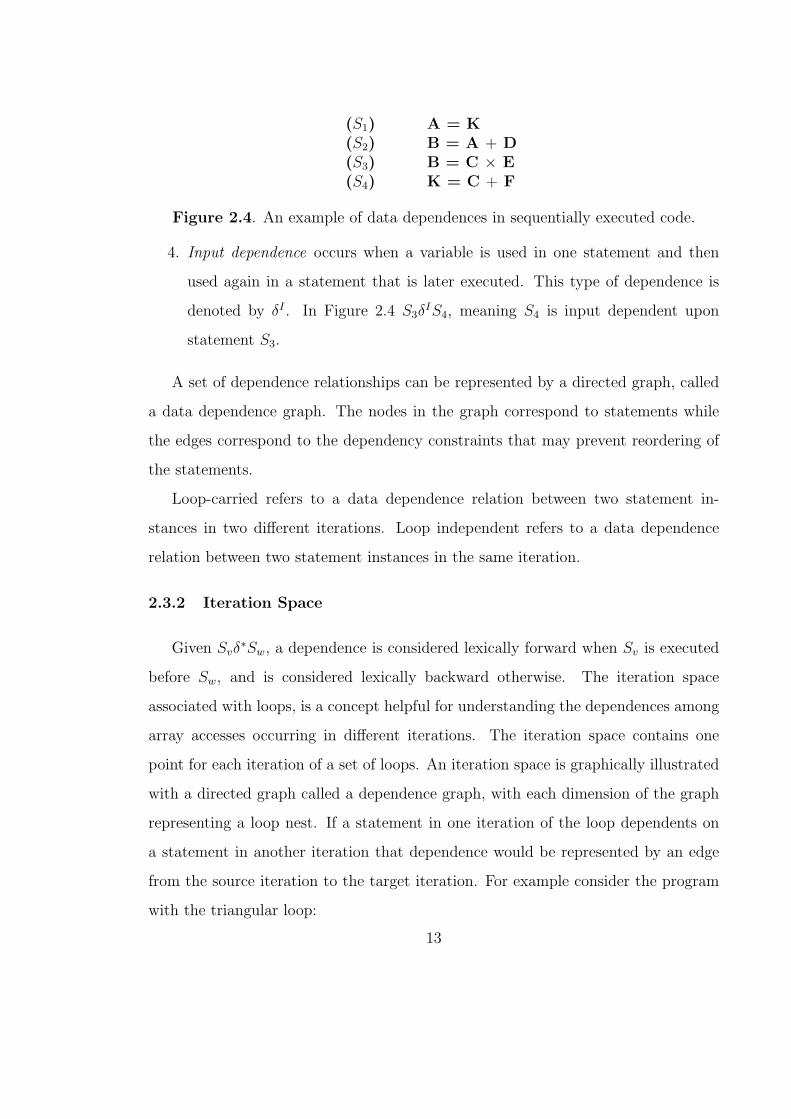
(S1) A = K(S2) B = A + D(S3) B = C × E(S4) K = C + F

Figure 2.4. An example of data dependences in sequentially executed code.

4. Input dependence occurs when a variable is used in one statement and then

used again in a statement that is later executed. This type of dependence is

denoted by δI . In Figure 2.4 S3δIS4, meaning S4 is input dependent upon

statement S3.

A set of dependence relationships can be represented by a directed graph, called

a data dependence graph. The nodes in the graph correspond to statements while

the edges correspond to the dependency constraints that may prevent reordering of

the statements.

Loop-carried refers to a data dependence relation between two statement in-

stances in two different iterations. Loop independent refers to a data dependence

relation between two statement instances in the same iteration.

2.3.2 Iteration Space

Given Svδ∗Sw, a dependence is considered lexically forward when Sv is executed

before Sw, and is considered lexically backward otherwise. The iteration space

associated with loops, is a concept helpful for understanding the dependences among

array accesses occurring in different iterations. The iteration space contains one

point for each iteration of a set of loops. An iteration space is graphically illustrated

with a directed graph called a dependence graph, with each dimension of the graph

representing a loop nest. If a statement in one iteration of the loop dependents on

a statement in another iteration that dependence would be represented by an edge

from the source iteration to the target iteration. For example consider the program

with the triangular loop:

13

Figure 2.5. An example showing loop iteration spaces. Here Graph A shows theiteration dependences for array B, while Graph B shows the iteration dependencesfor array D.

for (j = 2; j < 10; j = j + 2){

for (i = 0; i < j; ++i){

A[i] = B[i + 1]D[j, i + 1] = C[j] + F[j]B[i] = A[i] + D[j - 2, i]B[i] = C[j] * E[i]

}}

The directed dependence graph, associated with this code is shown in Figure 2.5.

The number of loop nest determine the dimensions of the graph. In this example,

with there being two nested loops, we need two dimensions in the dependence graph

to illustrate the iteration space. Notice that we have included two dependence graphs

in this example, one for dependences between array B and one for dependences for

array D.

14

Figure 2.6. An example showing normalized loop iteration spaces. Here GraphA shows the iteration dependences for array B, while Graph B shows the iterationdependences for array D.

2.3.3 Dependence Distances

Dependence distance is the vector difference between the iteration vectors of the

source and target iterations. The dependence distance will itself be a vector d,

called the distance vector, defined as d = it − is; where it is the target iteration

and is is the source iteration. It is important to note that the dependence distance

is not necessarily constant for all iterations. Figure 2.6 shows the iteration space

dependence graph with normalized iteration vectors. Many loop dependence analysis

test normalize iteration spaces in order to make dependence testing simpler.

2.3.4 Direction Vectors

Less precise than dependence distance are direction vectors. The symbols shown

in Table 2.1 are graphical symbols illustrating the ordering of vectors. For example

the ordering relation is < it indicates their is a lexically forward dependence between

the source and the target. The type of dependence is dependent on whether the

source is a def or a use, and on whether the target is a def or a use.

15

Table 2.1. Table showing direction vectors

< Crosses boundary forward= Doesn’t cross boundary> Crosses boundary backward≤ Occurs in the same iteration or forward≥ Occurs in the same iteration or backwards6= Cross an iteration boundary∗ Direction vector is unknown

2.3.5 Dependence Equations

A system of dependence equations is a system of linear equalities, or a system of

linear inequalities:

a11x1 + a12x2 + · · ·+ a1nxn � b1

a21x1 + a22x2 + · · ·+ a2nxn � b2

... =...

am1x1 + am2x2 + · · ·+ amnxn � bm

alternatively written in matrix notation as Ax � c, where � is either = or ≤, A is

the coefficient matrix composed of compile time constants, x is a vector of unknowns

composed of loop induction variables, and c is a vector of constants which represent

system constraints. In the case where the system is composed of linear inequalities,

when a variable appears with a positive coefficient, the inequality gives the upper

bound for the variable. Likewise, when a variable appears with a negative coefficient,

the inequality gives a lower bound for the variable. When a variable appears with

16

just a single nonzero coefficient, it is called a simple bounds. When a variable has

no upper bound or no lower bound it is called an unconstrained variable.

A system of linear inequalities describes a polytope. To solve a system of linear

inequalities, variables can be eliminated one at a time from the system by calculating

the shadow of the polytope when the polytope is projected along the dimension of

the variable we wish to eliminate. Later in this chapter we will look two techniques

for solving a system of linear inequalities Fourier-Motzkin variable elimination and

the Omega test, where Fourier-Motzkin variable elimination eliminates variables by

projecting real shadows, while the Omega test eliminates variables by projecting dark

shadows. There is an important difference in properties of real and dark shadows.

If a real shadow contains an integer point it doesn’t necessarily mean there is a

corresponding integer point located in the polytope described by the original system,

while if dark shadow contains an integer point, it will correspond to an integer point

located in the polytope described by the original system. Dark shadows are formed

from the part of the polytope which is at least one unit thick, while real shadows are

defined by no such constraints. As described in Wolfe[19] and Puge[14], the constraint

c2L ≤ c1U describes a real shadow, while the constraint c1U − c2L ≥ (c1− 1)(c2− 1)

defines a dark shadow, where c1 and c2 are the unknowns, U is the upper bound of

the shadow, and L is the lower bound of the shadow. Figure 2.7 provides a simple

illustration of dark and real shadows.

2.4 Dependence Analysis Systems

Compilers attempt to determine dependences by comparing subscript expressions

in loops. In order to do this the dependence analysis system must attempt to solve

a system of dependence equations and return its conservative findings. Essentially

there are three possible returns: has a solution, does not have a solution, or there

may be a solution. In this section, we will review four approaches to this problem.

17

Figure 2.7. Here a 2-dimensional polytope is defined by 3 linear equations. Inthis example we project the polytope along the y-axis and illustrate the differencebetween real and dark shadows. Notice that dark shadow is a subset of the realshadow, as it corresponds to the part of the polytope at least one unit thick.

We comment on each of their strengths and limitations. Also note that none of these

test are able to handle non-linear array indices when performing dependence analysis.

2.4.1 GCD Test

The Greatest Common Divisor(GCD) test is a well-known dependence analysis

test based on a theorem of elementary number theory which states that a linear

equation

a1x1 + a2x2 + a3x3 + . . . + anxn = b (2.1)

has an integer solution if and only if the greatest common divisor of the coefficients

a1, a2, a3, . . . , an, divides evenly into b. While the GCD test can detect independence,

when determining if there is a dependence, it returns inexact results in that it can

only determine if dependence is possible. Also the test indicates nothing about

18

dependence distances or direction. Furthermore, the greatest common divisor of all

the coefficients often turns out to be 1, in which case 1 will always divide evenly

into b. Despite these short comings however, it turns out determining the greatest

common divisor of two numbers is very inexpensive and easy to implement. For

this reason the GCD test often serves as a preliminary screening test to other more

complicated data dependence tests [9]. This screening is done to avoid analyzing

those array indices that could not possibly be dependent on one another such as the

following case illustrates:

for (i = 0; i < 10; i += 2){

A[i] = B[i + 1]D[i + 1] = A[i + 1]

}

Here the dependence equation would be 2id−2iu = 1. The GCD of the coefficients id

and iu is 2, which does not divided evenly into 1. In this example GCD determines

that there are no integer solutions and thus there can be no dependence.

2.4.2 Extreme Value Test

The extreme value test(EVT) is another well known dependence test. Sometimes

referred to as the Banerjee bounds test, it is based on the Intermediate Value Theorem

which states that if a continuous function takes on two values between two points, it

also takes on every value between those two points. This dependence test is inexact

because it can only determine if a real solution is possible but it is efficient and more

accurate than the GCD test. The test works by associating a lower and upper bound

for the left side of a dependence equation and then determining if dependence is

possible by determining if the value on right side of the equation lies between those

bounds. Traditionally in order to find the extreme value of a real number we use the

positive part r+ and r− of a number where:

19

r+ =

{0, r < 0r, r ≥ 0

r− =

{r, r ≤ 00, r > 0

hence in a dependence equation:

a1x1 + a2x2 + a3x3 + . . . + anxn = b (2.2)

the extreme values for the product of a variable and its coefficient, say for instance

a1x1 where L ≤ x ≤ U are represented by the lower bound:

a+1 L + a−1 U (2.3)

and the upper bound:

a+1 U + a−1 L (2.4)

as noted in [18].

In addition to determining if dependence is possible the EVT can also be used

to test for dependence in particular dependence directions. For instance as noted in

[17] to test for dependence in the direction id < iu where id represents a definition

of normalized induction variable i and iu represents a use of normalized induction

variable i, the upper bound for id can be replaced by iu − 1, or the lower bound for

iu can be replace by id + 1 with the algorithm followed as normal.

Essentially each equation has associated with it an upper bound and a lower

bound, and in order for dependence to be possible the constant on the right side

of the equation must lie between those bounds. In the case of an unknown having

no lower bound −∞ is the lower bound associated with equations containing the

unknown and likewise in the case of no upper bound for an unknown,∞ is the upper

bound associated with equations containing the unknown. Hence it is essential for

all unknowns to have at least one bound, whether it be upper or lower, associated

with it at compile time in order for this algorithm to be effective. Also note that with

20

triangular loop limits the test may return a false positive if there is a solution that

satisfies both the direction vector constraint and the loop limit constraint but not

both simultaneously. Here we show an example of using EVT to compute dependence

relations:

Consider the loop:

for (i = 0; i < 10; i += 1){

A[2i] = B[i + 6]D[i] = A[3i - 1]

}

With dependence equation:

2id − 3iu = −1

The upper bound and lower bound of both id and iu are computed as follows:

id = 2i iu = 3i= 2[0, 10] = 3[0, 10]= [0, 20] = [0, 30]

Which allow us to compute the upper and lower bounds for the dependence equation:

Lower Bound = 2id − 3iu Upper Bound = 2id − 3iu

= 2(0)− 3(30) = 2(20)− 3(0)= −90 = 40

Since -1 lies in the range of [-90,40] we know that dependence is a possibility.

2.4.3 Fourier-Motzkin Variable Elimination

Fourier-Motzkin Variable Elimination (FMVE), also Fourier-Motzkin Projection,

is a dependence analysis method that is often used as a basis for other dependence

analysis test. The test is able to determine if there are no real solutions for a system

of linear inequalities. The procedure works by systematically eliminating variables

21

from a system of inequalities until a contradiction occurs or all but a single variable

has been eliminated. For example, given a system of linear inequalities:

n∑j=1

aijxj ≥ bi, i = (1, . . . ,m) (2.5)

We can eliminate a variable xj by combining inequalities that describe its lower

bound and upper bound as follows:L ≤ c1xj

→ c2L ≤ c1Uc2xj ≤ U

(2.6)

Here L represents a lower bound for xj and U represents the upper bound and c1 and

c2 represents constants. Essentially FMVE works to find the n-1 dimensional real

shadow cast by an n dimensional object when variables are eliminated. By combining

the shadows of the intersection of each pair of upper and lower bounds a real shadow

of the original object is obtained.

The steps taken by the algorithm are listed below. Note that the steps are

repeated until all variables have been eliminated, or until a contradiction is reached.

1. A variable from the dependence equation is selected for elimination.

2. All inequalities of the dependence equations are rewritten in terms of the upper

and lower bounds for that variable.

3. New inequalities are derived that do not involve the variable selected for

elimination by comparing the lower bound with the upper bound for the

variable.

4. All the inequalities involving the variable are deleted, consequently the remain-

ing inequalities will be of one less variable.

If a contradiction is detected, or if there are no integer points in the real shadow

obtained, then dependence is not possible. If we are able to eliminate variables until

only one remains then dependence is possible.

22

When performing the algorithm as mentioned above it is useful to partition the

system of inequalities into three sets [7]:

D(x) : a′ix′i ≤ bi i = 1, . . . ,m1

E(x) : −x1 + a′jx′j ≤ bj, j = m1 + 1, . . . ,m2

F (x) : x1 + a′kx′k ≤ bk, k = m2 + 1, . . . ,m

(2.7)

where x’ is a vector containing all variables except that which is being eliminated,

a’ is a vector representing variable coefficients, and x1 is the variable which is being

eliminated. Each set D(x), E(x), and F (x) represents a partition of no bounds, lower

bounds, and upper bounds, respectively, for the variable x1. Equation 2.8 shows the

results of combining the lower and upper bounds of x1 to form new equations.

D(x) : a′i × x′ ≤ bi, i = 1, . . . ,m1a′j × x′ − bj ≤ bk − a′k × x′, j = m1 + 1, . . . ,m2

k = m2 + 1, . . . ,m(2.8)

Note that the process of FMVE can increase the number of inequalities exponentially

and is therefore at times not very efficient. Note also, with this test, the order in

which inequalities are eliminated makes a difference in exactness and performance.

Below we have include a simple example of FMVE using the equations shown in

Figure 2.7.

Consider the equations:

30y + x = 33027y − 7x = 84

27y − 10x = 81

We project out x, first expressing all inequalities as upper or lower bounds on x:

x ≤ −30y + 330−x ≤ −27

7y + 84

7

−x ≤ −2710

y + 8110

23

For any y, if there is an x that satisfies all the inequalities, then every lower bound

on x must be less than or equal to every upper bound on x. We eliminate x, and in

the process generate the following inequalities.

277y − 84

7≤ −30y + 330

2710

y − 8110≤ −30y + 330

Which leaves us with one unknown, y. The shadow of original region is given by

the line y ≤ 2394237

which is approximately 10, the tightest bound on y. Because we

have not run into any contradiction, we conclude that there are rational solutions to

the original system of inequalities, meaning dependence is a possibility.

2.4.4 Omega Test

The Omega test is an integer programming algorithm first introduced in [14]. It

is based on FMVE but it uses dark shadows, which are a subset of real shadows, to

determine if there is an integer solutions to a system of linear inequalities, and hence

is more accurate than FMVE. The main difference between the two tests is that

the Omega test works to find the shadows of the parts of the object thick enough,

i.e. at least one unit thick, to where there shadows must contain integer points

corresponding to the object the shadow is formed from. This change in technique

comes from the observation that there may be integer grid points in the shadow of

an object, even if though the object itself may contain no integer points.

24

CHAPTER 3

CHAINS OF RECURRENCES

Chains of Recurrences (CR’s) provide an efficient and compact means of repre-

senting functions on uniform grids. The formalism was first introduced as a means

to expedite the evaluation of closed-form functions at regular intervals. Polynomials,

rational functions, geometric series, factorials, trigonometric functions, and combi-

nations of the aforementioned are all efficiently represented by the CR notation.

In this Chapter we review the properties of CR’s as the CR notation provides the

mathematical basis for the induction variable substitution and dependence analysis

algorithms which we will present in subsequent chapters.

3.1 Chains of Recurrences Notation

Many compiler optimizations require the evaluation of closed-form functions at

various points within some interval. Specifically, given function F(x), starting point

x0, an increment h, and interval bounds i = 0, 1, . . . , n, we would like to find the value

for F(x0 + ih) over the range of i. Normally this type of evaluation is done recursively

where for each point on the grid represented by F(x), we must substitute in values

for all variables and evaluate the resulting expression, repeating the process from

scratch with each new point we wish to evaluate. Another more efficient approach to

this problem is instead of evaluating each point independently, take advantage of the

fixed relation defined between points on a regular grid and the value of the previous

point in order to compute the next. More specifically the function F can be rewritten

as a Basic Recurrence (BR) relation where:

25

f(i) =

{ι0, if i = 0f(i− 1)� g, if i > 0

(3.1)

with � ∈ {+, ∗}, g is a function defined over the natural numbers N, and ι0

representing an invariant. A more compact representation of equation 4.1 is

f(i) = {ι0,�, g}i (3.2)

where when substituting in the operators, + and ∗ for � we have the definitions,

{ι0, +, g}i = ι0 +i−1∑j=0

gj (3.3)

{ι0, ∗, g}i = ι0

i−1∏j=0

gj (3.4)

This BR notion is a simple representation of the first order linear recurrences shown

here:

f(0) = ι0

f(1) = ι0 � g(0)

f(2) = ι0 � g(0) � g(1)

f(3) = ι0 � g(0) � g(1) � g(2)...

f(i) = f(i-1) � g(i-1)

For all i > 0. This BR notion, which represents simple linear functions, can be

extended to represent more complex functions.

26

A closed-form function f can be rewritten as a mathematically equivalent

system of recurrence relations f0, f1, f2, . . . , fk, where the value of k depends on

the complexity of function f . Evaluating the function represented by fj for j =

0, 1, . . . , k − 1 within a loop with loop counter i, can be written as the recurrence

relation:

fj(i) =

{ιj, if i = 0fj(i− 1)�j+1 fj+1(i− 1), if i > 0

(3.5)

with �j+1 ∈ {+, ∗}, and ιj representing a loop invariant expression. Notice that

fk is not shown in equation 4.4; it is either a loop invariant expression or a similar

recurrence system. A more compact representation of equation 4.4 in which the BR

notation is extended is by writing g as a Chains of (Basic) Recurrences (CR’s) as

shown here:

Φi = {ι0,�1, {ι1,�2, . . . , {ιk−1,�k, g}i}i}i (3.6)

and also here flatten to a single tuple:

Φi = {ι0,�1, ι1,�2, . . . , ιk−1,�k, g}i (3.7)

Essentially BR’s are a simple case of CR’s in which g is represented by a constant

instead of another recurrence relation. CR’s are usually denoted by the Greek letter

Φ and that is the notation we will use throughout this thesis.

A CR Φ = {ι0,�1, ι1,�2, . . . ,�k, fk}i has the following properties:

- ι0, ι1, . . . , ιk are called the coefficients of Φ.

- k is called the length of Φ.

- if �j = + for all j = 1, 2, . . . , k, then Φ is called polynomial.

27

- if �j = ∗ for all j = 1, 2, . . . , k, then Φ is called exponential.

- if ik doesn’t not occur in the coefficients, then Φ is called regular.

- if Φ is regular and fk is a constant, then Φ is called simple.

3.2 CR Rewrite Rules

The CR formalism provides an efficient way of representing and evaluating

functions over uniform intervals. CRs and the expressions that contain them can be

manipulated through rewrite rules designed to either simplify the CR expression or

produce it’s equivalent closed form. These rewrite rules enable the development of an

algebra, such that the process of construction and simplification of CRs for arbitrary

closed-form functions can be automated within a symbolic computing environment

and hence are essential for algorithms we present later.

3.2.1 Simplification

The purpose of simplifying a CR expression is to produce an equivalent CR

expression that has the potential to be evaluated more efficiently. Bachmann[2]

categorizes CR simplification rules into the the four classes:

1. General - simplification rules that apply to all CR expressions.

2. Polynomial - simplification rules that apply to polynomial CR expressions.

3. Exponential - simplification rules that apply to exponential CR expressions.

4. Trigonometric - simplifications of CR expressions involving trigonometric

operators.

The simplification rules initially introduced in [20][21], given explicitly in [3] [22]

and then later extended in [2][15] are designed such that the rules enable the re-use of

28

Table 3.1. Chains of Recurrences simplification rules.

Expression Rewrite1. {ι0,+, 0}i =⇒ ι02. {ι0, ∗, 1}i =⇒ ι03. {0, ∗, f1}i =⇒ 04. −{ι0,+, f1}i =⇒ {−ι0,+,−f1}i5. −{ι0, ∗, f1}i =⇒ {−ι0, ∗, f1}i6. {ι0,+, f1}i ± E =⇒ {ι0 ± E,+, f1}i7. {ι0, ∗, f1}i ± E =⇒ {ι0 ± E,+, ι0 ∗ (f1 − 1), ∗, f1}i8. E ∗ {ι0,+, f1}i =⇒ {E ∗ ι0,+, E ∗ f1}i9. E ∗ {ι0, ∗, f1}i =⇒ {E ∗ ι0, ∗, f1}i10. E/{ι0,+, f1}i =⇒ 1/{ι0/E,+, f1/E}i11. E/{ι0, ∗, f1}i =⇒ {E/ι0, ∗, 1/f1}i12. {ι0,+, f1}i ± {ψ0,+, g1}i =⇒ {ι0 ± ψ0,+, f1 ± g1}i13. {ι0, ∗, f1}i ± {ψ0,+, g1}i =⇒ {ι0 ± ψ0,+, {ι0 ∗ (f1 − 1), ∗, f1}i ± g1}i14. {ι0,+, f1}i ∗ {ψ0,+, g1}i =⇒ {ι0 ∗ ψ0,+, {ι0,+, f1}1 ∗ g1+

{ψ,+, g1}i ∗ f1 + f1 ∗ g1}i15. {ι0, ∗, f1}i ∗ {ψ0, ∗, g1}i =⇒ {ι0 ± ψ0, ∗, f1 ∗ g1}i16. {ι0, ∗, f1}E =⇒ {ιE0 , ∗, fE1 }i17. {ι0, ∗, f1}{ψ0,+,g1}i

i =⇒ {ιψ00 , ∗, {ι0, ∗, f1}g1i ∗ f

{ψ0,+,g1}i1 ∗ fg11 }i

18. E{ι0,+,f1}i =⇒ {Eι0 , ∗, Ef1}i

19. {ι0,+, f1}ni =⇒{{ι0,+, f1}i ∗ {ι0,+, f1}n−1

i if n ∈ , n > 11/{ι0,+, f1}−ni if n ∈ , n < 0

20. {ι0,+, f1}i! =⇒

{{ι0!, ∗, (

∏f1j=1{ι0 + j,+, f1}i)}i if f1 ≥ 0

{ι0!, ∗, (∏|f1|j=1{ι0 + j,+, f1}i)−1}i if f1 < 0

21. {ι0,+, ι1, ∗, f1}i =⇒ {ι0, ∗, f2}i when ι1ι0 = f1 − 1

computational results obtained from previous evaluations. Mathematically speaking,

if we consider CRs as functions, then CR simplifications connect known algebraic

dependences of the domain values of CRs with dependences of the respective range

values. Table 3.1 shows the rewrite rules of interest as related to our implementations

of loop analysis and optimizations. Note that all the CR simplification rules are

applicable to CR’s representing both integer and floating point typed expressions.

29

3.2.2 CR Inverse

In [15], Van Engelen develops CR inverse rules (CR−1), designed to translate CR

expressions back to their equivalent closed-form. After application of the rules the

function that results must not contain any CRs as subexpressions. The CR inverse

system developed by Van Engelen can only derive a subset of closed form functions

corresponding to the CR expression since the mapping from closed form function

to CR is neither surjective nor one to one. However, mathematically speaking, the

mappings do return expressions equivalent to the domain of possible correct returns.

Table 3.2 shows the rewrite rules of interest as related to our implementations of loop

analysis and optimizations. Note as was the case with the CR simplification rules, all

the CR−1 rules are applicable to CR’s representing both integer and floating point

typed expressions. The transformation strategy for applying the CR−1 rules is to

reduce the innermost redexes first on nested CR tuples of the form equation 3. This

results in closed expressions for the increments in CR tuples which can be matched by

other rules. After the application of the inverse transformation CR−1, the resulting

closed form expression can be factorized to compress the representation.

3.3 An Example of Exploitation

Before we delve into any of the implementation details, we give an example

illustrating how CRs can be used to accelerate the evaluation of closed-form functions.

3.3.1 Exploitation

CRs afford an efficient method to accelerate the evaluation of closed-form func-

tions on regular grids by reusing values calculated at previous points. We consider

an iterative evaluation of a non-linear function over a number of regular points over

an interval.

30

Table 3.2. Chains of Recurrences inverse simplification rules.

Expression Rewrite1. {ι0,+, f1}i =⇒ ι0 + {0,+, f1}i2. {ι0, ∗, f1}i =⇒ ι0 ∗ {1, ∗, f1}i3. {0,+,−f1}i =⇒ −{0,+, f1}i4. {ι0,+, f1 + g1}i =⇒ {ι0,+, f1}i + {ι0,+, g1}i5. {ι0, ∗, f1 ∗ g1}i =⇒ f1 ∗ {ι0, ∗, g1}i6. {0,+, f i1}i =⇒ f i

1−1f1−1

7. {0,+, fg1+h11 }i =⇒ {0,+, fg11 ∗ f

h11 }i

8. {0,+, fg1∗h11 }i =⇒ {0,+, (fg11 )h1}i

9. {0,+, f1}i =⇒ i ∗ f1

10. {0,+, i}i =⇒ i2−i2

11. {0,+, in}i =⇒∑n

k=0(n+1

k )n+1 Bki

n−k+1

12. {1, ∗,−f1}i =⇒ (−1)i{1, ∗, f1}i13. {1, ∗, 1

f1}i =⇒ {1, ∗, f1}−1

i

14. {1, ∗, f1 ∗ g1}i =⇒ {1, ∗, f1}i ∗ {1, ∗, g1}i15. {1, ∗, fg11 }i =⇒ f

{1,∗,g1}i1

16. {1, ∗, gf11 }i =⇒ {1, ∗, g1}f1i17. {1, ∗, f1}i =⇒ f i118. {1, ∗, i}i =⇒ 0i

19. {1, ∗, i+ f1}i =⇒ (i+f1−1)!(f1−1)!

20. {1, ∗, f1 − 1}i =⇒ (−1)i ∗ (i−f1−1)!(−f1−1)!

Consider the polynomial:

p(x) = 2x3 + x2 + x + 9

which we would like to evaluate at the 21 points 0, .05, .10, . . . , .95, 1.00. In order

evaluate the polynomial, we generate the CR expression1:

Φ = 3 ∗ {0, +, .05}3 + {0, +, .05}2 + {0, +, .05}+ 9

Notice that Φ is similar to p, except that each occurrence of x in p is replaced by the

CR {0, +, .05}.1Algorithms for CR construction are described in [3], [22],[2]. In subsequent chapters we will

describe the algorithm given in [15] to be used in the induction variable substitution method

31

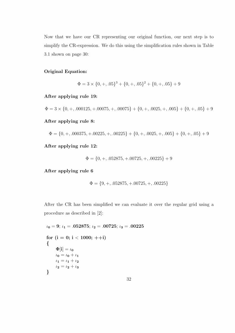
Now that we have our CR representing our original function, our next step is to

simplify the CR-expression. We do this using the simplification rules shown in Table

3.1 shown on page 30:

Original Equation:

Φ = 3× {0, +, .05}3 + {0, +, .05}2 + {0, +, .05}+ 9

After applying rule 19:

Φ = 3× {0, +, .000125, +.00075, +, .00075}+ {0, +, .0025, +, .005}+ {0, +, .05}+ 9

After applying rule 8:

Φ = {0, +, .000375, +.00225, +, .00225}+ {0, +, .0025, +, .005}+ {0, +, .05}+ 9

After applying rule 12:

Φ = {0, +, .052875, +.00725, +, .00225}+ 9

After applying rule 6

Φ = {9, +, .052875, +.00725, +, .00225}

After the CR has been simplified we can evaluate it over the regular grid using a

procedure as described in [2]:

ι0 = 9; ι1 = .052875; ι2 = .00725; ι3 = .00225

for (i = 0; i < 1000; ++i){

Φ[i] = ι0ι0 = ι0 + ι1ι1 = ι1 + ι2ι2 = ι2 + ι3

}32

Where Φi contains the values of p at the 21 points 0, .05, .10, . . . , .95, 1.00. Notice

that the computation of Φi requires just 3 additions per evaluation point where

normally we would of had to do an extra 21 multiplications. With any CR

Φi = {ι0,�1, ι1,�2, . . . , ιk−1,�k, g}i (3.8)

At most k additions or multiplications need to be performed at each loop iteration.

In later chapters we will see in detail how CR-expressions can be used to represent

recurrences and closed-form functions of loop induction variables to aid in induction

variable recognition and substitution, and dependence analysis.

3.4 A CR Framework

The exploitation of CRs in loop analysis and loop optimizations requires an

efficient and extensive framework based on the CR construct. The framework, in

turn, requires the implementation of CRs as an intermediate representation, the

implementation of a term rewriting system for both CR simplification and CR inverse,

and the development and implementation of various methods designed to aid in the

construction, simplification, and evaluation of CRs. We have used the second version

of Stanford University’s Intermediate Format (SUIF2) compiler infrastructure as our

reconstruction compiler. For our term rewriting system we choose to implement

functions in C in order to deal with compatibility and structural issues. For the

reminder of the this Chapter we examine our framework.

3.4.1 CR Implementation Representation

To avoid being too dependent upon any one compiler infrastructure, we use two

separate data structures to represent the CR notation. The first data structure

serves as an intermediate representation in SUIF2 and the second is written in C as

a conglomerate of structures and arrays.

33

#include "basicnodes/basic.hoof"

#include "suifnodes/suif.hoof"

module crexpr

{

include "basicnodes/basic.h";

include "suifnodes/suif.h";

include "pairsnodes/pairs.h";

import basicnodes;

import suifnodes;

import pairsnodes;

concrete CRSF : Expression

{

VariableSymbol * reference v;

int len;

int ref;

list<int> ops;

list<Expression * owner> coefficients;

};

}

Figure 3.1. SUIF2 Internal Representation for the CR notation

SUIF2, written in C++, is a modular based architecture, allowing for easy

extension of the intermediate representation. For our CR notation we wrote a simple

hoof2 file as seen in Figure 3.4.1, which created a CR expression module from the more

general expression already included in the SUIF2 infrastructure. Notice we have the

declarations, VariableSymbol v which represents the index variable of a CR, integer

len which represents the length of Φ, we have ref which is a simple flag indicating

if the CR is currently referenced, ops which is a list of �, where � ∈ {+, ∗}, and

coefficients which is a list of the coefficients Φ = {ι0,�1, ι1,�2, . . . ,�k, fk}i, where

k = len.

2For more information on the SUIF2 compiler infrastructure see ”The SUIF Programmer Guide”

34

CR-Driver Menu

------------------------------------------

1. Compute CR

2. Compute CR Inverse

3. Perform Induction Variable Substitution

4. Perform Dependence Anaylsis

5. Simple Bounds Checking

6. List Avaliable Input Files

7. Print Menu

8. Exit

Figure 3.2. CR-Driver Main Menu

For our C data structure representation of the CR notation we use arrays

encapsulated in structures to represent the ops and coefficients rather than linked

lists. The reason for this is to improve performance. Also two routines were

implemented, one that converts a CR expression written into a SUIF2 node, and

one that converts a CR SUIF2 node into a C expression.

3.4.2 The Expression Rewriting System

Our expression rewriting system is a mix of application of CR simplification rules

and constant folding. The CR simplification rules are the same as those seen in Table

3.1 and the constant folding rules are described in Appendix D.

3.4.3 A Driver

In order to test our framework we developed a small driver program ”CR-Driver”

as seen in Figure 3.2 and Figure 3.3. We use yacc and lex routines to scan and parse

input respectively.

35

Simplification Options

-----------------------

1. Verbose level ................ 1

2. Expanded Form ................ no

press ’x’ for exit or ’o’ for options.

-- to begin SIMPLIFY press enter.

Figure 3.3. CR-Driver Simplification Options Menu

36

CHAPTER 4

A CHAINS OF RECURRENCES IVS

ALGORITHM

Our implementation of the IVS algorithm was first presented by Van Engelen.

The algorithm recognizes both simple and generalized induction variables using the

CR framework, and then performs induction variable substitution. The algorithm

effectively removes all cross-iteration dependence induced by GIV updates, enabling

a loop to be parallelized. This Chapter presents the algorithm and and an imple-

mentation of it using the SUIF2 compiler system.

4.1 Algorithm

The CR based IVS algorithm is able to detect multiple induction variables in

loop hierarchies by using multivariate CRs. The algorithm, designed to be safe and

simple to implement, performs induction variable substitution on a larger class of

induction variables then existing ad hoc algorithms. Nine routines arranged in three

main components, make up the CR-based IVS algorithm. When analyzing loops the

algorithm supports sequences, assignments, if-then-else, do-loops, and while-loops.

The algorithm analyzes loop nests from the innermost to the outermost, removing

induction variable updates and replacing them with their closed forms. Pseudo-code

for the for the overall algorithm is shown in Figure 4.1. We discuss the routines,

SSA, CR, and HOIST, below.

37

Figure 4.1. Pseudocode for induction variable substitution (IVS) algorithm. HereS(L) denotes the loop body, i denotes the BIV of the loop, a denotes the loop bound,and s denotes the stride of the loop.

4.1.1 Conversion to SSA form

The first component of the IVS algorithm converts the body of every loop nest into

single-static assignment (SSA) form with assignments to scalar variables separated

from the body and stored in a set of variable-update pairs.

Figure 4.2 shows algorithm SSA. The algorithm defines a precedence relation on

variable-value pairs:

38

(U, Y ) � (V, X) if U 6= V and V occurs in Y

where U and V are the names of variables, in order to obtain a set of ordered

pairs taken from the loop body. The set of ordered pairs contain all the potential

induction variables of the loop, which are arranged in a directed acyclic graph for the

expressions of the pairs set. The algorithm saves space by storing the expressions in

such a way that common subexpressions share the same node in the graph. Notice in

the pseudo-code for the algorithm that both the if and else part of an if-else statement

are scanned for potential induction variables. Algorithm MERGE shown in Figure

4.3, merges the sets of potential induction variables. Notice also the algorithm fails

when � is not a partial order on the set of variable-value pairs. This occurs when

their are cyclic recurrences in the loop, something this algorithm cannot overcome.

4.1.2 GIV recognition

The second component of the IVS algorithm converts the expressions of the

variable-update pairs to CR-expressions so that the algorithm can detect BIV’s and

GIV’s. The algorithm utilizes the CR-simplification rules for CR construction of the

expressions.

Algorithm CR, shown in Figure 4.4 is constructs the CR for the expressions in the

variable-update pairs to obtain normalized CR-expressions. The CR’s are then used

to detect induction variables among the variable-update pairs. Notice the recognition

of wrap-around variables in the second else-if scope. Each use of a variable before its

definition is replaced by a CR-expression that represents the difference of value.

4.1.3 Induction Variable Substitution

The third component of the IVS algorithm performs the substitution of the

induction variable updates by their update’s closed forms. Algorithm Hoist shown

in Figure 4.5 hoist the induction variable assignments out of the loop and replaces

39

Figure 4.2. Shown here is Algorithm SSA, which is responsible for convertingvariable assignments to SSA form.

40

Figure 4.3. Shown here is Algorithm MERGE, which is responsible for merging thesets of potential induction variables found in both the if and else part of an if-elsestatement.

the induction variable expressions by their closed forms through the application of

CR-inverse rules.

4.2 Testing the Algorithm

Van Engelen created a prototype implementation of his IVS algorithm in the

CTADEL compiler system and illustrated its effectiveness with code segments from

MDG and TRFD, both of which are notorious for dependence between non-linear

expressions in different loop nest. We use the same code segments to test the

feasibility of a compiler implementation of the algorithm.

41

Figure 4.4. Shown here is Algorithm CR, which is responsible for convertingvariable-update pairs to CR form.

42

Figure 4.5. Shown here is Algorithm HOIST, which is responsible for removingloop induction variables and placing their closed-form outside of the loop.

4.2.1 TRFD

Certain code segments of TRFD from the Perfect Benchmark suite are difficult to

parallelize due to the presence of a number of coupled non-linear induction variables.

Figure 4.6 depicts the code segment of TRFD which we used to test the GIV

recognition method and the IVS algorithm.

The input for algorithm SSA is shown here:

Printing ForStatement Before ALGORITHM SSA 1

43

for (i = 0; i <= m; ++i)

{

for (j = 0; j <= i; ++j)

{

ij = ij + 1;

ijkl = ijkl + i - j + 1;

for (k = i + 1; k <= m; k++)

{

for (l = 1; l <= k; ++l)

{

ijkl = ijkl + 1;

xijkl[ijkl] = xkl[l];

}

}

ijkl = ijkl + ij + left;

}

}

Figure 4.6. The code segment from TRFD that we tested.

---------------------------------------------

for( l=1; l <= k; l+=1)

{

ijkl = (ijkl+1)

xijkl[ijkl] = xkl[l]

}

This is a code segment from the inner-most loop as the algorithm detects multi-

variant GIVs by working from the inner-most loop outward. The algorithm takes

the statement update for variable ijkl and stores it in the previously empty set of

variable-update pairs. The update to the array access of pointer xijkl is left to remain

in the loop as arrays are not candidates in our algorithm for induction variables.

However you may notice that the array indices has been transformed to its equivalent

CR form. The results of algorithm SSA:

44

Printing ForStatement Before ALGORITHM CR 1

--------------------------------------------

for( l=1; l <= k; l+=1)

{

xijkl[(ijkl+1)] = xkl[l]

}

Printing PairStruct Before ALGORITHM CR 1

------------------------------------------

0> ijkl = (ijkl+1)

serves as input to Algorithm CR. The CR algorithm converts the update expressions

in the set of variable-value pairs into normalized CR-expressions. This step detects

simple induction variable ijkl. Also the index expressions for xijkl and xkl are replaced

by their CR-expressions. The results of the CR algorithm are shown below:

Printing ForStatement Before ALGORITHM HOIST 1

-----------------------------------------------

for( l=1; l <= k; l+=1)

{

xijkl[{(1+ijkl),+,1}l] = xkl[{1,+,1}l]

}

Printing PairStruct Before ALGORITHM HOIST 1

------------------------------------------------

0> ijkl = {ijkl,+,1}l

Algorithm Hoist converts the CR-expressions in the set of variable-update pairs into

closed-form expressions by calling CR inverse. After algorithm Hoist, the variable

45

ijkl and its update are located outside of the original l loop. Notice that the

CR-expressions located in array indices are not touched until the final stage of the

IVS algorithm. The results of Algorithm Hoist are shown below:

Printing ForStatement After ALGORITHM Hoist 1

----------------------------------------------

for( l=0; l <= ((-1)+k); l+=1)

{

xijkl[{(1+ijkl),+,1}l] = xkl[{1,+,1}l]

}

ijkl = (ijkl+k)

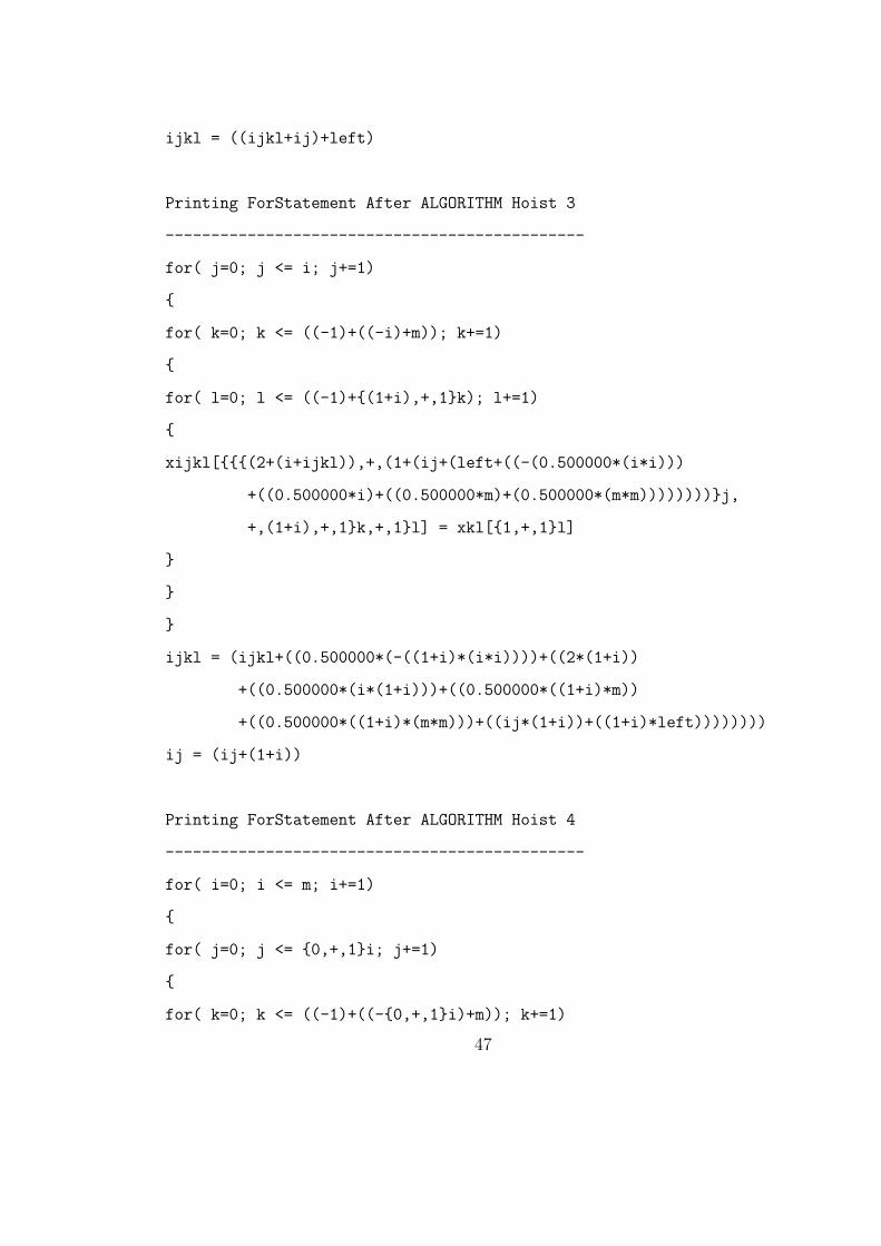
The algorithm then proceeds to analysis the next loop located beyond the one just

analyzed. Working further outwards the algorithm continues to hoist out GIVs. The

results seen below show the k, j, and i loop being analyzed respectively.

Printing ForStatement After ALGORITHM Hoist 2

----------------------------------------------

ij = (ij+1)

ijkl = (((ijkl+i)+(-j))+1)

for( k=0; k <= ((-1)+((-i)+m)); k+=1)

{

for( l=0; l <= ((-1)+{(1+i),+,1}k); l+=1)

{

xijkl[{{(1+ijkl),+,(1+i),+,1}k,+,1}l] = xkl[{1,+,1}l]

}

}

ijkl = (ijkl+((0.500000*((-i)+m))

+((0.500000*(((-i)+m)*((-i)+m)))+(i*((-i)+m)))))

46

ijkl = ((ijkl+ij)+left)

Printing ForStatement After ALGORITHM Hoist 3

----------------------------------------------

for( j=0; j <= i; j+=1)

{

for( k=0; k <= ((-1)+((-i)+m)); k+=1)

{

for( l=0; l <= ((-1)+{(1+i),+,1}k); l+=1)

{

xijkl[{{{(2+(i+ijkl)),+,(1+(ij+(left+((-(0.500000*(i*i)))

+((0.500000*i)+((0.500000*m)+(0.500000*(m*m))))))))}j,

+,(1+i),+,1}k,+,1}l] = xkl[{1,+,1}l]

}

}

}

ijkl = (ijkl+((0.500000*(-((1+i)*(i*i))))+((2*(1+i))

+((0.500000*(i*(1+i)))+((0.500000*((1+i)*m))

+((0.500000*((1+i)*(m*m)))+((ij*(1+i))+((1+i)*left))))))))

ij = (ij+(1+i))

Printing ForStatement After ALGORITHM Hoist 4

----------------------------------------------

for( i=0; i <= m; i+=1)

{

for( j=0; j <= {0,+,1}i; j+=1)

{

for( k=0; k <= ((-1)+((-{0,+,1}i)+m)); k+=1)

47

{

for( l=0; l <= ((-1)+{(1+{0,+,1}i),+,1}k); l+=1)

{

xijkl[{{{{(2+ijkl),+,(3+(ij+(left+((0.500000*m)

+((0.500000*(m*m))+(i*ij)))))),

+,(2+(ij+(left+((0.500000*m)+((0.500000*(m*m))

+(i*ij)))))),+,(ij+((i*ij)

+{(-3),+,(-3.000000)}i))}i,+,{(1+(ij+(left+((0.500000*m)

+(0.500000*(m*m)))))),+,1.000000}i}j,+,{1,+,1}i,+,1}k,+,1}l]

= xkl[{1,+,1}l]

}

}

}

}

ijkl = (ijkl+((-(0.125000*((1+m)*((1+m)*((1+m)*(1+m))))))

+((0.041667*(ij*((1+m)*(1+m))))+((0.041667*(ij*((1+m)

*((1+m)*((1+m)*(1+m))))))+((0.083333*(ij*((1+m)*((1+m)*(1

+m)))))+((0.250000*((1+m)*m))+((0.250000*(m*((1+m)*(1+m))))

+((0.250000*((1+m)*((1+m)*(1+m))))+((0.416667*(ij*((1+m)

*(1+m))))+((0.416667*((1+m)*ij))+((0.500000*((1+m)*left))

+((0.500000*((1+m)*(m*m)))+((0.500000*(left*((1+m)*(1+m))))

+((0.750000*(1+m))+((1.125000*((1+m)*(1+m)))+(((-(0.250000

*(1+m)))+(0.250000*((1+m)*(1+m))))*(m*m)))))))))))))))))

ij = (ij+((0.500000*(1+m))+(0.500000*((1+m)*(1+m)))))

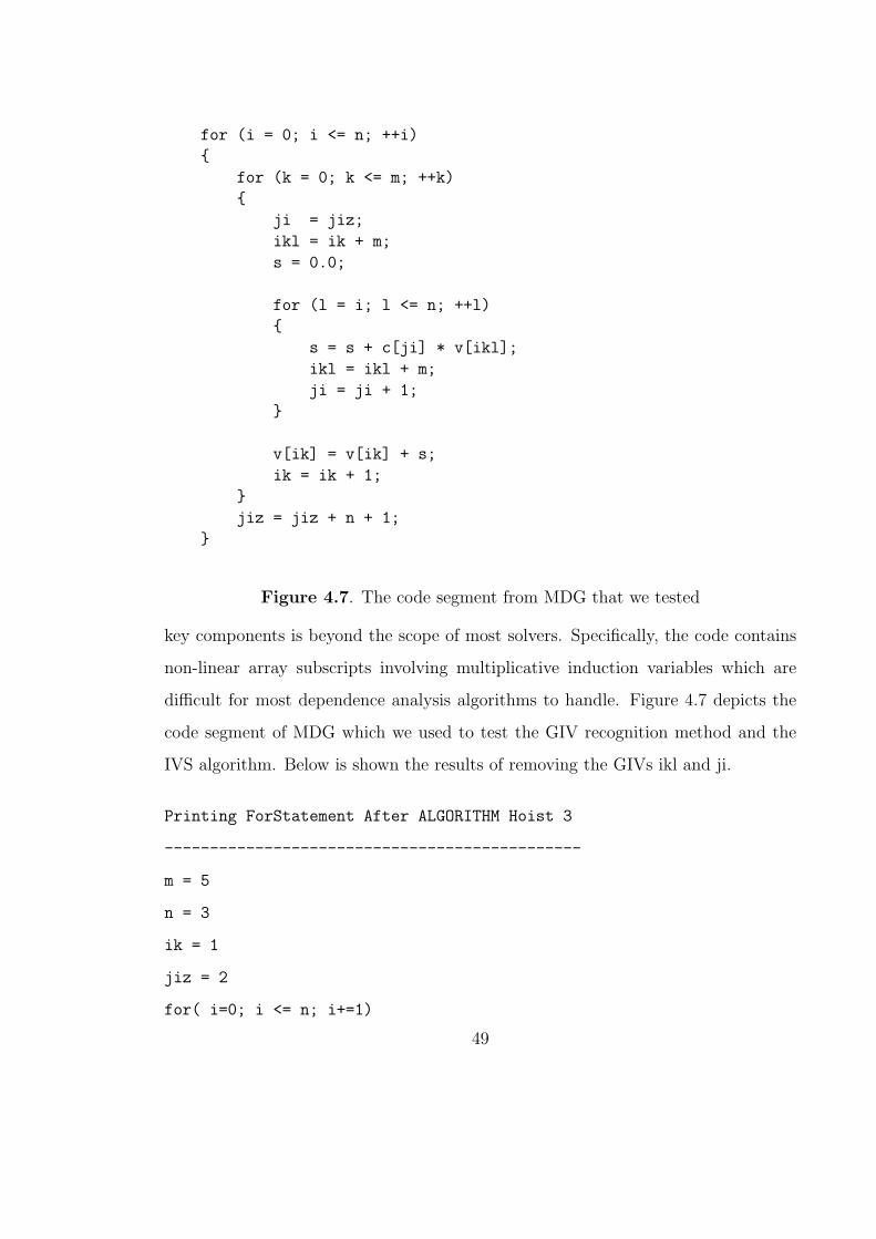
4.2.2 MDG

MDG from the Perfect Benchmarks suite contains key computational loops that

are safe to parallelize. Unfortunately performing proper dependence analysis on those

48

for (i = 0; i <= n; ++i)

{

for (k = 0; k <= m; ++k)

{

ji = jiz;

ikl = ik + m;

s = 0.0;

for (l = i; l <= n; ++l)

{

s = s + c[ji] * v[ikl];

ikl = ikl + m;

ji = ji + 1;

}

v[ik] = v[ik] + s;

ik = ik + 1;

}

jiz = jiz + n + 1;

}

Figure 4.7. The code segment from MDG that we tested

key components is beyond the scope of most solvers. Specifically, the code contains

non-linear array subscripts involving multiplicative induction variables which are

difficult for most dependence analysis algorithms to handle. Figure 4.7 depicts the

code segment of MDG which we used to test the GIV recognition method and the

IVS algorithm. Below is shown the results of removing the GIVs ikl and ji.

Printing ForStatement After ALGORITHM Hoist 3

----------------------------------------------

m = 5

n = 3

ik = 1

jiz = 2

for( i=0; i <= n; i+=1)

49

{

for( k=0; k <= m; k+=1)

{

s = 0.000000

for( l=0; l <= ((-{0,+,1}i)+n); l+=1)

{

s = (s+(c[{{jiz,+,(1+n)}i,+,1}l]*v[{({{ik,+,(1+m)}i,+,1}k+m),+,m}l]))

}

v[{{ik,+,(1+m)}i,+,1}k] = (s+v[{{ik,+,(1+m)}i,+,1}k])

}

}

ji = (1+((-n)+(jiz+(n+((1+n)*n)))))

jiz = ((1+n)+(jiz+((1+n)*n)))

ikl = ((-1)+((1+n)+(ik+((3*m)+(m*n)))))

ik = ((1+n)+(ik+((1+n)*m)))

Or testing shows that the algorithm is indeed able to cope with non-linear

expressions and improve upon the generalized induction variable recognition and

induction variable substitution algorithms.

50

CHAPTER 5

THE EXTREME VALUE TEST BY CR’S

CR’s afford an inexpensive method for determining the monotonicity of non-linear

functions. If monotonic analysis determines a function is increasing or decreasing

monotonically, efficient bounds analysis can be performed with the results utilized in

a non-linear dependence analysis test. In this Chapter we present the implementation

of a dependence analysis algorithm designed to take advantage of the efficiency

involved in analyzing the monotonic properties of a CR.

5.1 Monotonicity

A monotonic function is a function which is either entirely non-increasing or

nondecreasing. A characteristic of this type of function is that its first derivative

(which need not be continuous) does not change sign. If a function is known to be

monotonic, then value range analysis can be performed on the function and utilized

in non-linear dependence analysis test. For this reason monotonicity forms a basis

for non-linear dependence analysis.

If a function f(x) is known to be monotonically increasing, it has its greatest value

at the largest value of x and its lowest value at the smallest value of x. Conversely

if a function f(x) is known to be monotonically decreasing, it has its greatest value

at the smallest value of x and its lowest value at the smallest value of x. Traditional

methods used for determining maximum and minimum values deal strictly with linear

functions because determining the monotonicity of non-linear functions is expensive,

and more importantly can return incorrect results. For example consider value range

51

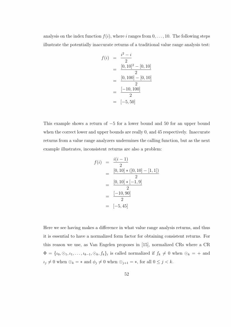
analysis on the index function f(i), where i ranges from 0, . . . , 10. The following steps

illustrate the potentially inaccurate returns of a traditional value range analysis test:

f(i) =i2 − i

2

=[0, 10]2 − [0, 10]

2

=[0, 100]− [0, 10]

2

=[−10, 100]

2

= [−5, 50]

This example shows a return of −5 for a lower bound and 50 for an upper bound

when the correct lower and upper bounds are really 0, and 45 respectively. Inaccurate

returns from a value range analyzers undermines the calling function, but as the next

example illustrates, inconsistent returns are also a problem:

f(i) =i(i− 1)

2

=[0, 10] ∗ ([0, 10]− [1, 1])

2

=[0, 10] ∗ [−1, 9]

2

=[−10, 90]

2

= [−5, 45]

Here we see having makes a difference in what value range analysis returns, and thus

it is essential to have a normalized form factor for obtaining consistent returns. For

this reason we use, as Van Engelen proposes in [15], normalized CRs where a CR

Φ = {ι0,�1, ι1, . . . , ιk−1,�k, fk}i is called normalized if fk 6= 0 when �k = + and

ιj 6= 0 when �k = ∗ and φj 6= 0 when �j+1 = ∗, for all 0 ≤ j < k.

52

5.1.1 Monotonicity of CR-Expressions

Determining the monotonicity of CRs is simple, efficient, and fast. If all the

coefficients of a CR are non-negative, the CR is considered positive and monotonically

increasing. Similarly if all the coefficients are negative the CR is considered negative

and monotonically decreasing. That is a CR

Φ = {ι0,�1, ι1,�2, . . . ,�k, fk}i (5.1)

has a positive monotonicity if for all j, where 0 ≤ j < k and fk ≥ 0, where fk

represents a CR. The lower bound L of a CR Φ = {ι0,�1, ι1,�2, . . . ,�k, fk}i is it’s

initial value ι0 if it is monotonically increasing. The upper bound U is obtained by

deriving the closed-form of the CR by applying the CR−1 rules.

5.2 Algorithm

The CR loop analysis method constructs CR-expressions for arbitrary index

expressions and simplifies them by using CR simplification rules. From the resulting

CRs, a fast and effective method of linear and non-linear index dependence testing

performs dependence analysis using direction vectors. The CR test, based on the

extreme value test, expands the former’s solution space by solving for both linear

and non-linear expressions in dependence equations.

The algorithm, pseudo code for which is seen in Figure 5.1, first seeks out an

outer most loop. The loop is then normalized. Next for each statement in the loop,

the loop induction variable is renamed to label it as begin used in conjunction with

a definition or a use. Next the algorithm constructs CR-expressions for the arbitrary

index expressions found in each statement of the loop. Then system of dependence

equations is formed by removing the CR-expressions from the array subscripts of

each statement, CR simplification is performed, and any remaining CR is moved

to the left side of the dependence equation with any remaining constants moving

53

Figure 5.1. Shown here is Algorithm EVT, which is responsible for merging thesets of potential induction variables found in both the if and else part of an if-elsestatement.

to the right. From here the algorithm determines the lower and upper bounds of

the CR-expressions and compares the result with the constant on the right side of

the equation. If the constant lies between the lower and upper bound range then

the algorithm determines dependence is possible and continues on to determine the

direction(s) in which it is possible by using the direction vector hierarchy. After the

algorithm finishes determining dependence with a loop it tries to see if it has any

inner loops and determines dependence based for low limits of both loops.

As is the case with the traditional extreme value test, our algorithm finds

the extreme values of an expression with unknowns located on the left side of a

dependence equations, then determines if dependence is possible by comparing the

expression’s range with the constant located on the right hand side of the dependence

54

equation. Also like the extreme value test a direction vector hierarchy is used to

determine the kind and direction of any possible dependences by applying direction

vector constraints.

5.3 Implementation

Needed for the CR loop analysis algorithm are two methods, one that determines

the lower bound of a CR-Expression and one that determines the upper bound.

In order for these methods to make definitive returns for CR-Expressions which

represent non-linear functions, another method which determines the monotonicity

of a CR is needed to cater to the lower and upper bound methods.

We implemented the routines for determining the lower bound, upper bound,

and monotonicity of a CR-expression in C, outside of SUIF2. With SUIF2 we simply

created a routine that find loops from the inner most outward, and pass them to

another function that would normalize the loop, labeling unknowns as defs or uses,

and then create a dependence equation. From here a routine test dependence based

on the direction vector hierarchy, only testing nodes in hierarchy who’s parents

indicated a possible dependence. Table B.1 in Appendix B shows the function

mappings for lower bound, upper bound, and monotonicity routines implemented

for the algorithm. Our CR monotonicity testing is performed in O(k) time, where k

is the degree of the polynomial.

To give you an idea of how the Min Max, and Monotonicity functions operate

the Table B.1 in appendix B shows their function mappings. A CR-expression with

annotated unknowns is passed to the Min and Max functions with a range for the

loop iteration variable, and they return the min and max of the those CR-expressions

respectively.

55

Orginal Loop

------------

for( I=1; I <= 10; I+=1)

{

for( J=1; J <= 10; J+=1)

{

a[((I*I)+J)] = 0

b[1] = a[(((I*10)+J)+(-1))]

b[3] = b[(I*3)]

}

}

Figure 5.2. The original loop

5.4 Testing the Algorithm

Testing the CR dependence algorithm to verify that its analysis range covers that

of both linear and non-linear subscript expressions, appropriate code was generated

and passed to the CREVT routine. The actions and results of the program executing

on that code are outlined in this section.

The original code is shown in Figure 5.2. The code was generated not only to

test the algorithms ability to handle non-linear subscripts such as the first statement

of the innermost loop, but also to test the algorithms ability to compute dependence

between subscripts with more than one unknown.

The loop dependence testing is performed on the inner most loop first, working

its way outward loop by loop. In the case of the loop in Figure 5.2 the loop with

induction variable j is passed to the CREVT routine first. From here Figure 5.3 shows

the results of the loop being normalized. Notice also it shows all the unknowns within

the loop have been renamed appropriately depending on whether it is located on the

left side (def) or the right side (use) of the equation. From this point dependence

equations with the unknowns encapsulated in CRs are defined as mentioned in the

algorithm above.

56

Normalized Loop

---------------

for( J=0; J <= 9; J+=1)

{

a[((I*I)+(J_def+1))] = 0

b[1] = a[(((I*10)+(J_use+1))+(-1))]

b[3] = b[(I*3)]

}

Figure 5.3. The inner most loop is normalized.

Dependence Testing

------------------

Loop: (J)

Direction: (*)

Testing Arrays: a[((I*I)+(J_def+1))] = a[(((I*10)+(J_use+1))+(-1))]

Dependence Equation: ({(1+(I*I)),+,1}J_def+{(-(10*I)),+,(-1)}J_use) = 0

Upperbound: Undefined

Lowerbound: Undefined

Possible Dependence: Yes

Direction: (*)

Testing Arrays: b[1] = b[(I*3)]

Dependence Equation: (1+(-(3*I))) = 0

Upperbound: Undefined

Lowerbound: Undefined

Possible Dependence: Yes

Direction: (*)

Testing Arrays: b[3] = b[(I*3)]

Dependence Equation: (3+(-(3*I))) = 0

Upperbound: Undefined

Lowerbound: Undefined

Possible Dependence: Yes

Figure 5.4. Dependence testing of the innermost loop

57

Normalized Loop

---------------

for( I=0; I <= 9; I+=1)

{

for( J=0; J <= 9; J+=1)

{

a[(((I_def+1)*(I_def+1))+(J_def+1))] = 0

b[1] = a[((((I_use+1)*10)+(J_use+1))+(-1))]

b[3] = b[((I_use+1)*3)]

}

}

Figure 5.5. SUIF2 Internal Representation for the CR notation

From this point, the J def and J use, have been annotated with there appropriate

lower and upper bounds based on the normalized loop index variable J, but the

variable I has been annotated with nothing as its bounds are unknown at this time1.

The algorithm precedes operating on limited information and tries to determine

dependence for each possible conflict between a set and a use, the results of which

are shown in Figure 5.4.

Figure 5.4 shows the algorithm returning that there is a possibility of dependence

between the three potential conflicts. This return however did not take into account

the bounds of the variable I. At this point the algorithm, the algorithm is obviously

returning conservative returns due to limited information. When the algorithm

reaches a point where it can analysis the outer most loop, the range of I will be known

and more accurate dependences will be shown, while traditional extreme value test

will still be forced to make a conservative return on the dependency involving the

access to array A, due to the non-linear expression associated with its dependence

equation.

1This can be done by annotating the symbol table with scope dependent bounds information,but this has not been done in our implementation

58

Direction: (*,*)

Testing Arrays: a[(((I_def+1)*(I_def+1))+(J_def+1))]

= a[((((I_use+1)*10)+(J_use+1))+(-1))]

Dependence Equation: ({0,+,(-1)}J_use+({0,+,(-10)}I_use

+({0,+,1}J_def+{0,+,3,+,2}I_def))) = 8

Upperbound: 40

Lowerbound: -99

Possible Dependence: Yes

Figure 5.6. Dependence test in (∗, ∗) direction of array a

After the J-loop has finished going through its dependence analysis the I-loop

is next in line for its turn. Figure 5.5 shows the results of this loop being

normalized, with loop induction variable I being replaced throughout the loop with

the appropriate I def and I use variables which are both annotated with lower and

upper bounds for I. Notice at this point the J def and J use variable remain and

remain annotated. The next step in the loop is to set up the dependence equations,

which again, is done as mentioned in the algorithm above.

Testing the dependence between reference to array a, we see from Figure 5.6 that

in the (∗, ∗) direction the algorithm was able to produce lower of -99 and an upper

bound of 40 for the non-linear equation on the left side of the dependence equation.

Since 8, the constant on the right, lies between 40 and -99, the algorithm return there

is a possible dependence and continues on deeper in the dependence hierarchy to try

and discover the direction of the dependence.

Figure 5.7 shows that in the (<, ∗) direction there is no dependence, and since

there is no dependence at this point in the hierarchy the direction vectors (<,<),

(<, =), and (<,>) need not be tested and the algorithm moves on to test other

direction vectors.

Figure 5.8 shows testing dependence in the (=, ∗) direction produces a possible

dependence return. So from here the algorithm tries to pinpoint the exact dependence

direction which is shown to be in (=, >) direction.

59

Direction: (<,*)

Testing Arrays: a[(((I_def+1)*(I_def+1))+(J_def+1))]

= a[((((I_use+1)*10)+(J_use+1))+(-1))]

Dependence Equation: ({0,+,(-1)}J_use+({0,+,(-10)}I_use

+({0,+,1}J_def+{0,+,3,+,2}I_def))) = 8

Upperbound: 3

Lowerbound: -99

Possible Dependence: NO

Figure 5.7. Dependence test for (<, ∗) direction of array a.

Figure 5.9 shows that dependence exist in all three directions (>,<), (>, =), and

(>,>). The reminder of the dependency checks done for array b, are not shown, but

they were also done.

From the above results we see how the monotonicity of CR’s allows for a fast and

efficient method of using the extreme value test to find dependences between array

indices even if those indices can non-linear expressions. The method expands the

solution space for the extreme value test.

5.5 IVS integrated with EVT

In the previous Chapter we saw how CR-expressions can be used to represent

recurrences and closed-form functions of loop induction variables to aid in induction

variable recognition and substitution. The IVS algorithm however, can be run as

an initial step to EVT analysis. The benefits of merging the two algorithm into one

is that by performing IVS first, we are able to minimize the amount of work that

needs to be done by EVT by removing updates and already having BIV’s, GIV’s

and potential multi-variant CR-expressions already in their CR forms. The following

code is used to illustrates this interaction:

The Original Code Segment:

60

Direction: (=,*)

Testing Arrays: a[(((I_def+1)*(I_def+1))+(J_def+1))]

= a[((((I_use+1)*10)+(J_use+1))+(-1))]

Dependence Equation: ({0,+,(-1)}J_use+{0,+,1}J_def) = 8

Upperbound: 9

Lowerbound: -9

Possible Dependence: YES

Direction: (=,<)

Testing Arrays: a[(((I_def+1)*(I_def+1))+(J_def+1))]

= a[((((I_use+1)*10)+(J_use+1))+(-1))]

Dependence Equation: ({0,+,(-1)}J_use+{0,+,1}J_def) = 8

Upperbound: -1

Lowerbound: -9

Possible Dependence: NO

Direction: (=,=)

Testing Arrays: a[(((I_def+1)*(I_def+1))+(J_def+1))]

= a[((((I_use+1)*10)+(J_use+1))+(-1))]

Dependence Equation: 0 = 8

Upperbound: 0

Lowerbound: 0

Possible Dependence: NO

Direction: (=,>)

Testing Arrays: a[(((I_def+1)*(I_def+1))+(J_def+1))]

= a[((((I_use+1)*10)+(J_use+1))+(-1))]

Dependence Equation: ({0,+,(-1)}J_use+{0,+,1}J_def) = 8

Upperbound: 9

Lowerbound: 1

Possible Dependence: YES

Figure 5.8. Testing dependence in the (=, ∗) direction.

61

Direction: (>,*)

Testing Arrays: a[(((I_def+1)*(I_def+1))+(J_def+1))]

= a[((((I_use+1)*10)+(J_use+1))+(-1))]

Dependence Equation: ({0,+,(-1)}J_use+({0,+,(-10)}I_use

+({0,+,1}J_def+{0,+,3,+,2}I_def))) = 8

Upperbound: 40

Lowerbound: -61

Possible Dependence: YES

Direction: (>,<)

Testing Arrays: a[(((I_def+1)*(I_def+1))+(J_def+1))]

= a[((((I_use+1)*10)+(J_use+1))+(-1))]

Dependence Equation: ({0,+,(-1)}J_use+({0,+,(-10)}I_use

+({0,+,1}J_def+{0,+,3,+,2}I_def))) = 8

Upperbound: 30

Lowerbound: -61

Possible Dependence: YES

Direction: (>,=)

Testing Arrays: a[(((I_def+1)*(I_def+1))+(J_def+1))]

= a[((((I_use+1)*10)+(J_use+1))+(-1))]

Dependence Equation: ({0,+,(-10)}I_use+{0,+,3,+,2}I_def) = 8

Upperbound: 31

Lowerbound: -52

Possible Dependence: YES

Direction: (>,>)

Testing Arrays: a[(((I_def+1)*(I_def+1))+(J_def+1))]

= a[((((I_use+1)*10)+(J_use+1))+(-1))]

Dependence Equation: ({0,+,(-1)}J_use+({0,+,(-10)}I_use

+({0,+,1}J_def+{0,+,3,+,2}I_def))) = 8

Upperbound: 40

Lowerbound: -51

Possible Dependence: YES

Figure 5.9. Testing for dependence in the (>, ∗) direction.

62

k = 0for (i = 0; i < 10; ++i){

for (j = 0; j < i; ++j){

A[k] = A[(10*i) + j]k = k + 1

}}

is given to the SSA algorithm. After performing generalized induction variable

recognition and substitution the following code is produce:

for (i = 0; i < 10; ++i){

for (j = 0; j < i; ++j){

A[{{0,+,1,+,1}i,+,1}j] = A[{{0,+,10}i,+,1}j]}

}

Notice here that we leave the expressions of the array access in CR notion. From

here the code produced by SSA can be passed to EVT to produce the code:

for (i = 0; i < 10; ++i){

for (j = 0; j < i; ++j){

A[{{0,+,1,+,1}i def,+,1}j def] = A[{{0,+,10}i use,+,1}j use]}

}

and the dependence equation for the (*,*) direction:

{{0,+,1,+,1}i def,+,1}j def + {{0,+,-10}i use,+,-1}j use = 0

in order to determine possible dependence.

63

CHAPTER 6

CONCLUSIONS

6.1 Conclusions

We have developed and implemented efficient and effective techniques to analyze

induction variables and data dependences, to transform code based on those analysis.

We have demonstrated on examples from the Perfect Club Benchmark Suite, and

toy examples containing non-affine functions, the enhanced capabilities of these

algorithms. Through the design and implementation of a self-contained library we

have demonstrated the feasibility of a restructuring system based on these techniques.

We conclude that the implementations of loop analysis techniques based on the

chains of recurrence representation are not only feasible and practical, but also highly

advantageous.

6.2 Future Work

We believe the CR representation will aid in future enhancements to loop

strength reduction, code motion, program equivalence testing, program correctness

verification, and worst case execution time (WCET). Through utilization of our

developed CR framework, we feel that many advance can be made high performance

and parallel computing.

64

APPENDIX A

CONSTANT FOLDING

The following transformations define our constant folding rules. X, Y , and Z arearbitrary expressions, while N , M , and K are all constants.

Table A.1: Constant Folding Rules.

Expression RewriteAddition Rules

1. 0 +X =⇒ X2. X + (−X) =⇒ 03. X +X =⇒ X4. (N ×X) +X =⇒ (K ×X) where K = N + 15. (N ×X) + (−X) =⇒ (K ×X) where K = N − 16. (N ×X) + (M ×X) =⇒ (K ×X) where K = N +M

Multiplication Rules7. (0×X) =⇒ 08. (X ×X) =⇒ X9. (X × (1/X)) =⇒ 110. (X ×X) =⇒ (X2)11. (XN ×X) =⇒ (XK) where K = N + 112. (XN × (1/X)) =⇒ (XK) where K = N − 113. (XN ×XM ) + (M ×X) =⇒ (XK) where K = N +M

Exponentiation Rules14. X1 =⇒ X15. X−1 =⇒ (1/X)16. X0 =⇒ 117. 0X =⇒ 018. 1X =⇒ X

19. 1/(XY ) =⇒ (X(−Y ))20. (1/X)Y =⇒ (X(−Y ))21. (XY )Z =⇒ (X(Y×Z))

CR Rules22. {X,�, Y,�, Z,�, . . . ,+, 0} =⇒ {X,�, Y,�, Z,�, . . .}

– Continued –65

Table A.1: – Continued –

23. {X,�, Y,�, Z,�, . . . ,×, 1} =⇒ {X,�, Y,�, Z,�, . . .}24. {0,�, Y,�, Z,�, . . .} =⇒ 025. −{X,�, Y,�, Z,�, . . .} =⇒ {−X,�,−Y,�,−Z,�, . . .}

Distributive Rules26. −(X + Y + Z + . . .) =⇒ (−X) + (−Y ) + (−Z) + . . .27. 1/(X × Y × Z × . . .) =⇒ 1/((1/X)× (1/Y )× (1/Z)× . . .)28. ((−X)× Y × Z × . . .) =⇒ −(X × Y × Z × . . .)29. (X × (Y × Z)) =⇒ (X × Y ) + (X × Z)

66

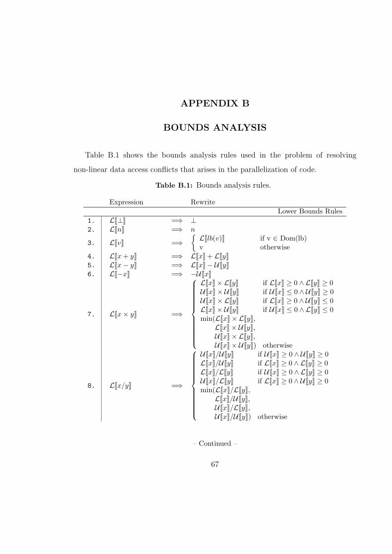
APPENDIX B

BOUNDS ANALYSIS

Table B.1 shows the bounds analysis rules used in the problem of resolving

non-linear data access conflicts that arises in the parallelization of code.

Table B.1: Bounds analysis rules.

Expression RewriteLower Bounds Rules

1. LJ⊥K =⇒ ⊥2. LJnK =⇒ n

3. LJvK =⇒{LJlb(v)K if v ∈ Dom(lb)v otherwise

4. LJx+ yK =⇒ LJxK + LJyK5. LJx− yK =⇒ LJxK− UJyK6. LJ−xK =⇒ −UJxK

7. LJx× yK =⇒

LJxK× LJyK if LJxK ≥ 0 ∧ LJyK ≥ 0UJxK× UJyK if UJxK ≤ 0 ∧ UJyK ≥ 0UJxK× LJyK if LJxK ≥ 0 ∧ UJyK ≤ 0LJxK× UJyK if UJxK ≤ 0 ∧ LJyK ≤ 0min(LJxK× LJyK,LJxK× UJyK,UJxK× LJyK,UJxK× UJyK) otherwise

8. LJx/yK =⇒

UJxK/UJyK if UJxK ≥ 0 ∧ UJyK ≥ 0LJxK/UJyK if LJxK ≥ 0 ∧ LJyK ≥ 0LJxK/LJyK if UJxK ≥ 0 ∧ LJyK ≥ 0UJxK/LJyK if LJxK ≥ 0 ∧ UJyK ≥ 0min(LJxK/LJyK,LJxK/UJyK,UJxK/LJyK,UJxK/UJyK) otherwise

– Continued –

67

Table B.1: – Continued –

9. LJxnK =⇒

LJxKn if n ≥ 0 ∧ LJxK ≥ 0UJxKn if n < 0 ∧ LJxK > 0UJxKn if n ≥ 0 ∧ n mod 2 = 0

∧ UJxK < 0LJxKn if n ≥ 0 ∧ n mod 2 = 1

∧ UJxK < 0LJxKn if n < 0 ∧ n mod 2 = 0

∧ UJxK < 0UJxKn if n < 0 ∧ n mod 2 = 1

∧ UJxK < 0min(LJxKn,UJxKn) otherwise

10. LJx÷ yK =⇒{

(LJxK− n+ 1)/n if n > 0UJxK/n if n < 0

11. LJx%nK =⇒{

0 if LJxK ≥ 01 - |n| otherwise

12. LJmax(x, y)K =⇒ max(LJxK,LJyK)13. LJmin(x, y)K =⇒ min(LJxK,LJyK)14. LJbxcK =⇒ LJxK− 115. LJdxeK =⇒ LJxK

16. LJΦK =⇒

LJι0K if LJMi(Φi)K ≥ 0LJCR−1

i (Φi)[i←U(i)]K if UJMi(Φi)K ≤ 0LJCR−1

i (Φi)K otherwiseUpper Bounds Rules

17. UJ⊥K =⇒ ⊥18. UJnK =⇒ n

19. UJvK =⇒{UJU(v)K if v ∈ Dom(U)v otherwise

20. UJx+ yK =⇒ UJxK + UJyK21. UJx− yK =⇒ UJxK− LJyK22. UJ−xK =⇒ −LJxK

23. UJx× yK =⇒

UJxK× LJyK if UJxK ≤ 0 ∧ LJyK ≥ 0LJxK× UJyK if LJxK ≥ 0 ∧ UJyK ≤ 0LJxK× LJyK if UJxK ≤ 0 ∧ UJyK ≤ 0UJxK× UJyK if LJxK ≥ 0 ∧ LJyK ≥ 0max(LJxK× LJyK,LJxK× UJyK,UJxK× LJyK,UJxK× UJyK) otherwise

– Continued –

68

Table B.1: – Continued –

24. UJx/yK =⇒

LJxK/UJyK if LJxK ≥ 0 ∧ UJyK < 0UJxK/UJyK if UJxK ≤ 0 ∧ LJyK > 0UJxK/LJyK if LJxK ≥ 0 ∧ LJyK > 0LJxK/LJyK if UJxK ≤ 0 ∧ UJyK < 0max(LJxK/LJyK,LJxK/UJyK,UJxK/LJyK,UJxK/UJyK) otherwise

25. UJxnK =⇒

LJxKn if n < 0 ∧ LJxK > 0UJxKn if n ≥ 0 ∧ LJxK ≥ 0LJxKn if n ≥ 0 ∧ n mod 2 = 0

∧ UJxK < 0UJxKn if n ≥ 0 ∧ n mod 2 = 1

∧ UJxK < 0LJxKn if n < 0 ∧ n mod 2 = 1

∧ UJxK < 0UJxKn if n < 0 ∧ n mod 2 = 0

∧ UJxK < 0max(LJxKn,UJxKn) otherwise

26. UJx÷ yK =⇒{UJxK/n if n > 0(LJxK− n+ 1)/n if n < 0

27. UJx%nK =⇒{

0 if UJxK ≤ 01 - |n| otherwise

28. UJmax(x, y)K =⇒ max(UJxK,UJyK)29. UJmin(x, y)K =⇒ min(UJxK,UJyK)30. UJbxcK =⇒ UJxK31. UJdxeK =⇒ UJxK + 1

32. UJΦK =⇒

UJι0K if UJMi(Φi)K ≤ 0UJCR−1

i (Φi)[i←U(i)]K if LJMi(Φi)K ≥ 0UJCR−1

i (Φi)K otherwiseMonotoncity Rules

33. Mi({ι0,+, f1}i) =⇒ f1

34. Mi({ι0, ∗, f1}i) =⇒

f1 − 1 if LJι0K ≥ 0 ∧ LJf1K > 01− f1 if LJι0K ≤ 0 ∧ LJf1K > 0⊥ otherwise

35. Mi({ι0,�1, f1}j) =⇒ Mi(ι0)

Here L represents the lowerbound function and U represents the upperbound

function. The Max and Min functions return respectively the maximum and

minimum values of an Expression or of a CR-Expression. Results returned are based

69

on induction variable extremes for monotonic functions and constant information.

The ⊥ symbol represents that a return value is unknown.

70

REFERENCES

[1] Allen, F., Cocke, J., and Kennedy, K. Reduction of operator strength.In Program Flow Analysis: Theory and Applications, S. Muchnick and N. Jones,Eds. Prentice-Hall Inc. Englewood Cliffs New Jersey, 1981, ch. 3, pp. 79–101.

[2] Bachmann, O. Chains of recurrences. PhD thesis, 1997.

[3] Bachmann, O., Wang, P. S., and Zima, E. V. Chains of recurrences -a method to expedite the evaluation of closed-form functions. In InternationalSymposium on Symbolic and Algebraic Computation (1994), pp. 242–249.

[4] Briggs, P., and Cooper, K. D. Effective partial redundancy elimination. InSIGPLAN Conference on Programming Language Design and Implementation(1994), pp. 159–170.

[5] Cocke, J., and Kennedy, K. An algorithm for reduction of operatorstrength. Communications of the ACM 20, 11 (1977), 850–856.

[6] Cooper, K. D., Simpson, L. T., and Vick, C. A. Operator strengthreduction. Programming Languages and Systems 23, 5 (2001), 603–625.

[7] George .B. Dantzig, B. C. E. Fourier-motzkin elimination and its dual.Journal of Combinatorial Theory 14, 14 (1973), 288–297.

[8] Goff, G., Kennedy, K., and Tseng, C.-W. Practical dependence testing.In Proceedings of the ACM SIGPLAN ’91 Conference on Programming LanguageDesign and Implementation (Toronto, Ontario, Canada, June 1991), vol. 26,pp. 15–29.

[9] Gupta, R., Pande, S., Psarris, K., and Sarkar, V. Compilationtechniques for parallel systems. Parallel Computing 25, 13–14 (1999), 1741–1783.

[10] Haghighat, M. R., and Polychronopoulos, C. D. Symbolic analysisfor parallelizing compilers. ACM Transactions on Programming Languages andSystems 18, 4 (July 1996), 477–518.

[11] Knoop, J., Ruething, O., and Steffen, B. Lazy code motion. InProceedings of the ACM SIGPLAN ’92 Conference on Programming Language

71

Design and Implementation (San Francisco, CA, June 1992), vol. 27, pp. 224–234.

[12] Knoop, J., Ruthing, O., and Steffen, B. Optimal code motion: Theoryand practice. ACM Transactions on Programming Languages and Systems 16,4 (July 1994), 1117–1155.

[13] Psarris, K., and Kyriakopoulos, K. Measuring the accuracy and effi-ciency of the data dependence tests. In International Conference on Paralleland Distributed Computing Systems (2001).

[14] Pugh, W. The omega test: a fast and practical integer programming algorithmfor dependence analysis. In Supercomputing (1991), pp. 4–13.

[15] van Engelen, R. Symbolic evaluation of chains of recurrences for loopoptimization, 2000.

[16] van Engelen, R. A. Efficient symbolic analysis for optimizing compilers.Lecture Notes in Computer Science 2027 (2001).

[17] Wolfe, M. High Performance Compilers for Parallel Computing. AddisonWesley, Redwood City, CA, 1996.

[18] Wolfe, M., and Banerjee, U. Data dependence and its application toparallel processing. International Journal of Parallel Programming 16, 2 (1987),137–178.

[19] Wolfe, M. J. Optimizing Supercompilers for Supercomputers. MIT Press,1990.

[20] Zima, E. V. Automatic construction of systems of recurrence relations.USSR Computational Mathematics and Mathematical Physics 24, 11-12 (1986),193–197.

[21] Zima, E. V. Recurrent relations and speed-up of computations using computeralgebra systems. In Proc. of DISCO, Bath, U.K., April 1992 (1992), pp. 152–161.

[22] Zima, E. V. Simplification and optimization transformations of chains of re-currences. In International Symposium on Symbolic and Algebraic Computation(1995), pp. 42–50.

72

BIOGRAPHICAL SKETCH

Johnnie L. Birch

Johnnie Birch graduated from Florida State University in the Fall of 1999 with a

B.S. degree in Meteorology. He worked for a educational outreach group in the

meteorology department until he went back to school in the Fall of 2000 to pursue

a Masters in Computer Science. While attending to earning his degree he became

a member of Upsilon Pi Epsilon, honor Society in the Computer Science, and a

member of ACM. Since 2001 he has been a research assistant for his major professor,

Dr. Robert Van Engelen.

73