USING INTERFEROMETRIC SYNTHETIC APERTURE RADAR DATA … · USING INTERFEROMETRIC SYNTHETIC APERTURE RADAR DATA TO ... Zebker is the best co-advisor a girl could ask for. ... Dan Aukes,

USING INTERFEROMETRIC SYNTHETIC

APERTURE RADAR DATA TO

IMPROVE ESTIMATES OF HYDRAULIC HEAD

IN THE SAN LUIS VALLEY, COLORADO

A DISSERTATION

SUBMITTED TO THE DEPARTMENT OF GEOPHYSICS

AND THE COMMITTEE ON GRADUATE STUDIES

OF STANFORD UNIVERSITY

IN PARTIAL FULFILLMENT OF THE REQUIREMENTS

FOR THE DEGREE OF

DOCTOR OF PHILOSOPHY

Jessica Anne Reeves

March 2013

ii

© Copyright by Jessica Reeves 2013

All Rights Reserved

iii

I certify that I have read this dissertation and that, in my opinion, it is fully

adequate in scope and quality as a dissertation of Doctor of Philosophy.

__________________________________

(Rosemary Knight) Principal Advisor



__________________________________

(Howard Zebker)



__________________________________

(Mark Zoback)

Approved for the University Committee on Graduate Studies.

__________________________________

iv

Abstract

Remotely sensed Interferometric Synthetic Aperture Radar (InSAR) deformation data

have recently been used to study confined aquifer systems in urban/arid areas. The

deformation measured at the surface by InSAR is a consequence of changes in hydraulic

head in the underlying confined aquifer system. Deformation in agricultural areas, such

as the San Luis Valley, Colorado, is difficult to measure using InSAR because changes in

the height of the vegetation can degrade the measurement by altering the positions of

individual radar scatterers. Nonetheless, agricultural areas like the San Luis Valley are of

great interest because of the link between the groundwater resources and the local

economy.

The San Luis Valley is an 8000 km2 valley, located mostly on the northern side of the

Colorado-New Mexico border. The valley has a vibrant agricultural economy that is

highly dependent on the effective management of limited water resources. State

regulation established that hydraulic head levels within the confined aquifer system

should be maintained within the range experienced in the years between 1978 and 2000.

v

Effective management of water resources in the San Luis Valley requires both seasonal

changes in hydraulic head as well long term trends during this time period.

In this study we had three main goals: 1) to determine if high quality InSAR data can be

collected in the San Luis Valley, 2) to determine the uncertainty of the InSAR

deformation measurements, and 3) to determine to what extent the InSAR deformation

data can be used to improve estimates of hydraulic head in the San Luis Valley.

We found that high quality InSAR data could be acquired from the San Luis Valley.

Many small areas, left unwatered by the center-pivot irrigation systems, yield high

quality InSAR data when processed using Small Baseline Subset analysis. The InSAR

deformation measurements showed the same seasonal periodicity as the hydraulic head

data from monitoring wells. Because no other ground-based deformation measurements

have been made in the San Luis Valley we decided to use InSAR data and aquifer test

data to estimate hydraulic head. We found good agreement between the estimated

hydraulic head values and the measured head values made at wells (within the error bars

of the head estimates). However, we acknowledge that using aquifer test data in the

analysis led to errors in the hydraulic head estimates that were too large to provide the

level of accuracy required for effective groundwater management.

The next step in our research was to more accurately determine the uncertainty in the

InSAR deformation measurements. Addressing the uncertainty in InSAR measured

deformation is critical if these data are to be used for groundwater applications as a basis

vi

for management decisions. We developed a novel algorithm that uses supplementary

hydrologic data to identify InSAR acquisitions whose measurements may have been

corrupted with uncertainty due to atmospheric phase effects. We then proceeded to

quantify the uncertainty in the InSAR deformation measurement due to decorrelation of

radar signals. Finally, we determined how to set Small Baseline Subset analysis

thresholds in order to achieve an acceptable level of uncertainty for a given application.

In this way groundwater managers can provide an ideal level of uncertainty and the

deformation data can be processed accordingly.

In the final chapter of this work we explored ways in which the relationship between

InSAR measured deformation and measurements of hydraulic head can be combined to

increase the spatial and temporal density of hydraulic head measurements in the confined

aquifer system. Unlike previously studied aquifer systems, where attempts were made to

match the deformation predicted by a transient groundwater flow models to the InSAR

measured deformation, we focused on estimating the parameter most important for

groundwater managers in the San Luis Valley, the hydraulic head. We showed how and

when we can improve the estimates of hydraulic head by exploring the relationship

between the spatially and temporally dense InSAR deformation data and the sparse

hydraulic head measurements. We found that at three well locations where the changes in

hydraulic head were sufficiently large and the aquifer sediments were relatively

compressible the InSAR deformation measurements can be reliably used to estimate

hydraulic head during times when no well measurements were acquired.

vii

Acknowledgments

Going to graduate school was hands down the best decision I ever made.

Not because of all the amazing groundbreaking science I have done, I use the word

groundbreaking loosely of course, but because of all the amazing people that have

helped me along the way. Stanford is a place of humans helping humans make

discoveries.

The one and only Rosemary Knight is to thank for making me the scientist I am

today. Although my writing skills are still in progress, as shown in this thesis, I can

only hope that some of her other amazing abilities have rubbed off on me. Howard

Zebker is the best co-advisor a girl could ask for. He has an amazing ability to tell

you that your work is completely wrong without making you feel terrible; a real

perk in an advisor. Willem Schreuder and Eric Harmon were the best collaborators

on Earth. They answer emails at all times of the day, any day of the week. I would

also like to say thanks to Mark Zoback, one of my committee members from the

beginning. Although Mark has very little experience in the world of hydrogeology

viii

he was always able to pick out the flaw in my scientific reasoning. And last but not

least, Peter Kitanidis, without your classes and help with the final chapter of this

thesis I am sure I would still be processing data right now, so thank you.

Almost more important than the technical support was the emotional support that

was provided by the people around me. Most importantly Katherine Dlubac and

Denys Grombacher, who always knew what I was going through better than

anyone. A special thanks to my past officemates Annemarie Baltay and Justin

Brown. Needless to say, best office ever. However, topping all the people at

Stanford are my dearest of friends: Dan Aukes, Mike Stern, Kristen Ericksson and

Zach Brown. Let me just say, stay classy and thanks for stopping by.

If anyone is to thank for me both starting and finishing this Ph.D. it is my parents.

They yelled at me until they were blue in the face to leave Toronto for California,

and luckily I went. They made me appreciate how lovely it is to work on

challenging and new problems every day. I would also like to un-thank my brother

David for beating me out of school, way to make an older sister feel bad. And

finally, thank you David Cameron. From day 1 to day 1944 you saw it all, and

made sure I toughed it out.

Funding for my research has come from a number of sources: the Stanford School

of Earth Sciences, the Nelson Award, and NASA. Thank you so much for making a

philosophical doctor out of me.

ix

Contents

Abstract iv

Acknowledgments vii

Contents ix

List of Figures xii

List of Tables xv

Chapter 1: Introduction 1

1.1 Problem definition, groundwater in the San Luis Valley 1

1.2 Motivation, the use of remotely sensed data 3

1.3 Objectives and contributions 6

Chapter 2: Theoretical background 8

2.1 InSAR background 8

2.1.1 InSAR imaging of deformation 8

2.1.2 Uncertainty in InSAR deformation measurement 14

2.1.3 Small Baseline Subset (SBAS) analysis 19

2.2 Aquifer deformation background 25

2.2.1 Theoretical definitions 25

2.2.2 Coupled hydromechanical systems 33

x

Chapter 3: Overview of available data 36

3.1 Introduction to field site 36

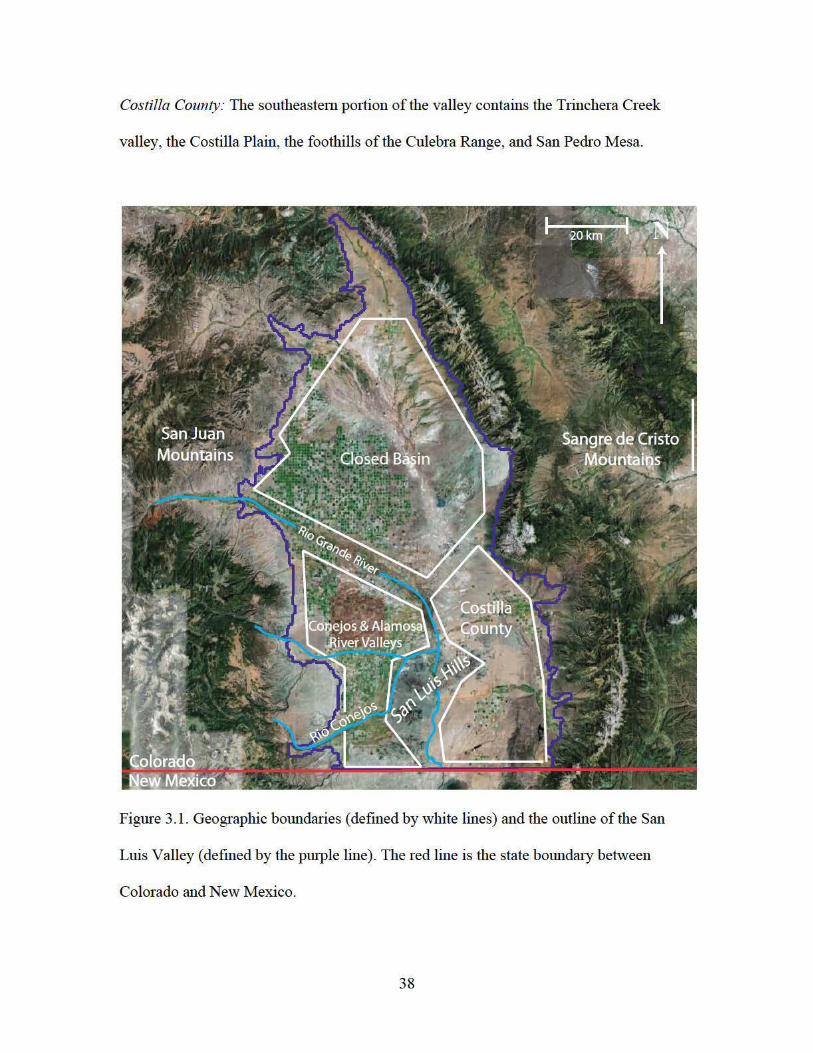
3.2 Hydrogeologic data 39

3.2.1 Hydrogeologic layers 39

3.2.2 Aquifer parameters 43

3.3 Hydraulic head data 44

3.4 Synthetic Aperture Radar (SAR) data 45

Chapter 4: Assessment of hydraulic head data 48

4.1 Review of hydraulic head data 48

4.1.1 Spatial sampling of hydraulic head data 49

4.1.2 Temporal sampling of hydraulic head data 52

4.2 Predicted deformation 54

Chapter 5: Assessment of InSAR deformation data 58

5.1 Introduction 58

5.2 Converting from deformation to hydraulic head 60

5.3 The Small Baseline Subset and interferograms 61

5.4 The mean coherence and SBAS thresholds 64

5.5 SBAS analysis modified for groundwater applications 67

5.6 Comparison of LOS time series and hydraulic head time series 69

5.7 Head estimates from InSAR deformation and aquifer test data 74

5.8 Conclusions 78

Chapter 6: Quantifying uncertainty in the InSAR measurement 81

6.1 Introduction 81

6.2 Atmospheric uncertainty in the SLV 85

6.2.1 Method 87

6.2.2 Results and discussion 88

6.3 Propagation of uncertainty due to decorrelation 92

6.3.1 Uncertainty in the interferometric phase 92

xi

6.3.2 Propagating uncertainty through SBAS analysis 93

6.3.3 Propagating the uncertainty of the SLV InSAR data 99

6.4 Uncertainty and SBAS analysis thresholds 104

6.4.1 Method 104

6.4.2 Results and discussion 105

6.5 Conclusions 109

Chapter 7: Improved estimates of hydraulic head 112

7.1 Introduction 112

7.2 Relationship between head and deformation around three wells 116

7.2.1 Linear regression analysis 117

7.2.2 Variability of Ske around wells: ALA6, ALA7 and ALA8 118

7.2.3 Uncertainty in the InSAR deformation measurements and R2 120

7.3 Spatial analysis of deformation data and hydraulic head data 123

7.3.1 Geostatistical definition of the variogram 124

7.3.2 Semi-variogram analysis of Δd 127

7.3.3 Semi-variogram analysis of Δh 137

7.4 Comparison of hydraulic head data and deformation data at wells 138

7.4.1 Performing Simple Kriging 139

7.4.2 Linear regression of kriged deformation data and head data 140

7.4.3 Predicting hydraulic head at wells ALA6, ALA7 and ALA8 147

7.5 Conclusions 149

Chapter 8: Conclusions 153

7.1 Summary of research 153

7.3 Future directions 157

References 161

xii

List of Figures

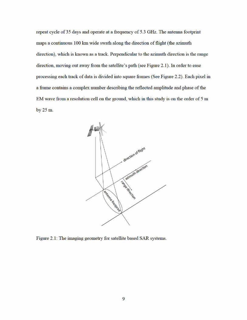
2.1 SAR satellite imaging geometry ............................................................................. 9

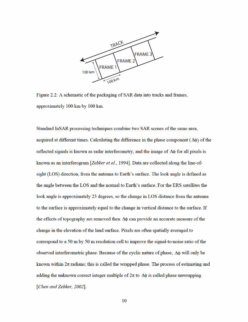
2.2 Schematic of SAR tracks and frames ................................................................... 10

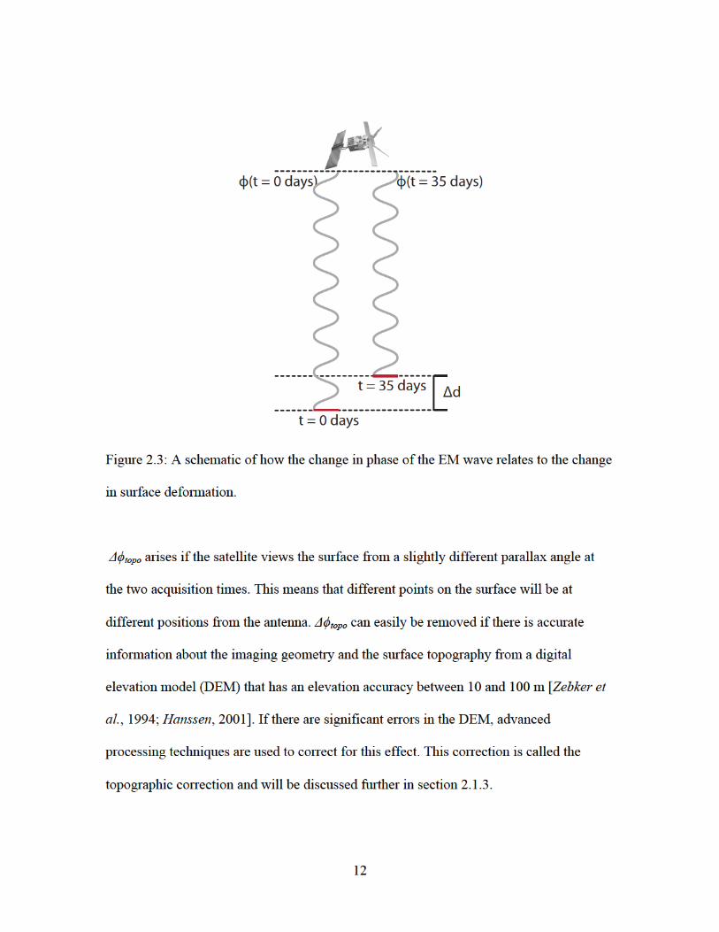
2.3 Change in phase of EM wave to deformation ...................................................... 12

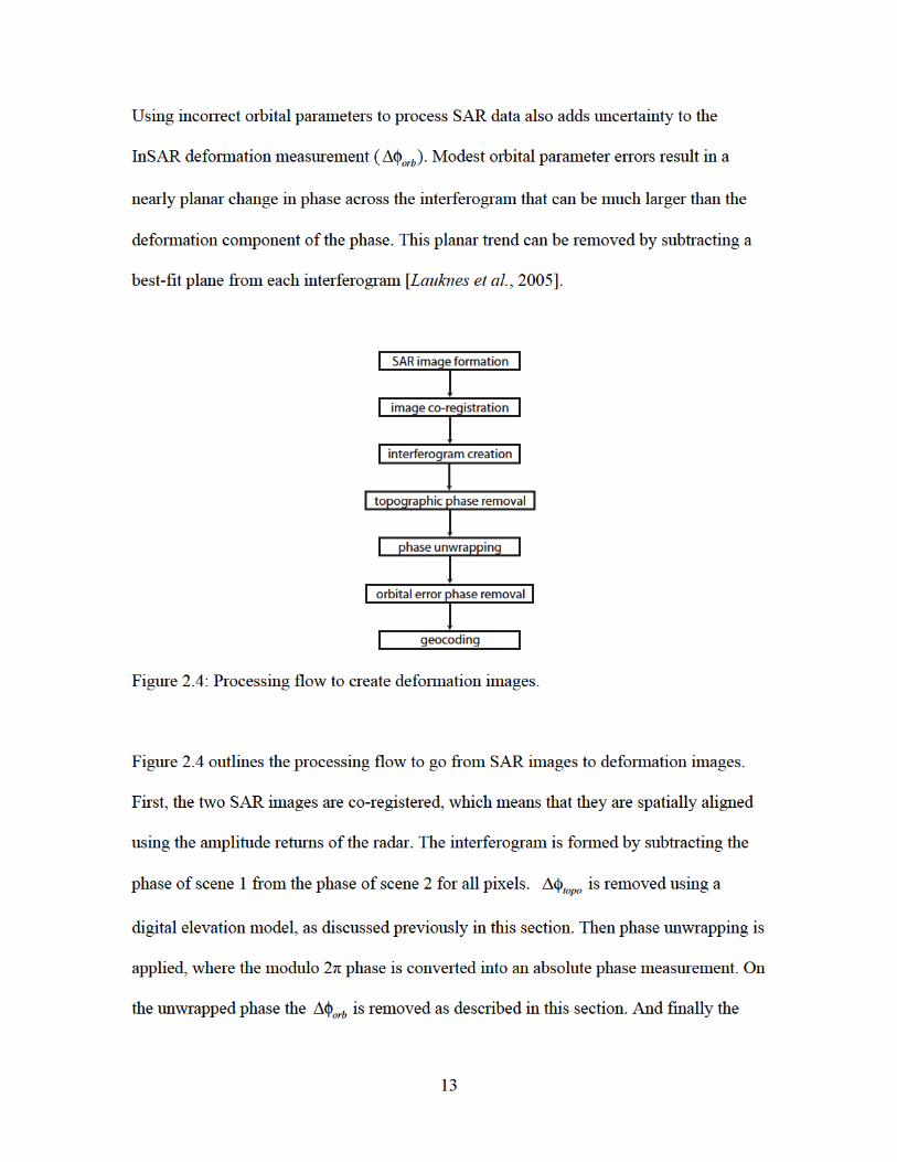
2.4 InSAR processing flow ......................................................................................... 13

2.5 SBAS example time-baseline plot ........................................................................ 20

2.6 Conventional SBAS analysis algorithm ............................................................... 24

2.7 Typical movement of water in valley aquifer system ........................................... 33

2.8 Schematic of flow when aquitard and aquifer equilibrated .................................. 34

2.9 Schematic of flow when aquitard and aquifer unequilibrated .............................. 35

3.1 Geographic boundaries of the SLV ...................................................................... 38

3.2 Schematic of variable geology in the SLV ........................................................... 39

3.3 Cross-section of hydrogeologic layers in the SLV ............................................... 42

3.4 Outline of SAR data in the SLV ........................................................................... 46

4.1 Location and quantity of hydraulic head data ...................................................... 50

4.2 Monitoring layers for hydraulic head data ........................................................... 51

4.3 Hydraulic head temporal filtering example .......................................................... 53

4.4 Location of 15 wells sampling confined aquifer system ...................................... 55

xiii

5.1 Time-baseline plot for ERS data in the SLV ........................................................ 62

5.2 Interferogram Nov. 1999 to July 2000 ................................................................. 63

5.3 Mean coherence over the entire SLV ................................................................... 65

5.4 Zoom in of mean coherence ................................................................................. 66

5.5 Hydraulic head time series for CON2 .................................................................. 68

5.6 Modified SBAS analysis for groundwater applications ....................................... 69

5.7 Line-of-sight deformation time-series and hydraulic head time-series ................ 71

5.8 Map of SLV showing locations of collocated wells and aquifer tests .................. 72

5.9 Estimated and measure hydraulic head time-series .............................................. 77

6.1 Quality of InSAR data in arid/urban areas vs. vegetated areas ............................ 82

6.2 Interpolated deformation with atmospheric phase effects .................................... 87

6.3 Example of algorithm used to remove atmospheric phase effects ....................... 88

6.4 Results from atmospheric algorithm with synthetic data ..................................... 90

6.5 Results from atmospheric algorithm with real data .............................................. 91

6.6 Coherence vs. standard deviation of interferometric phase ................................. 101

6.7 Line-of-sight deformation with propagated uncertainty ..................................... 101

6.8 Mean standard deviation of deformation over entire SLV ................................. 103

6.9 Standard deviation of deformation vs. mean coherence (vary # ints) ................ 106

6.10 Standard deviation of deformation vs. mean coherence (vary coh std) ….......... 107

6.11 Standard deviation of deformation vs. mean coherence (SLV data) .................. 108

7.1 Schematic of spatially variable deformation uncertainty in vegetated areas ...... 114

7.2 Schematic of kriged deformation estimates around a well ................................. 115

7.3 The spatial distribution of Ske estimates around wells ……………………......... 119

7.4 Relationship between R2, uncertainty and distance to well ALA6 …………...... 121



7.7 Schematic of a semi-variogram model ……………………………..…….......... 126

7.8 Experimental variogram and model for deformation data …………………....... 128

7.9 2D variogram for deformation data …………………………………..……....... 131

xiv

7.10 Semi-variograms and models for deformation data …………………….…....... 133




7.14 Semi-variograms for hydraulic head data ……………………………….…....... 137

7.15 Linear regression results for ALA6, ALA7 and ALA8 …………….….............. 142

7.16 Measured and estimated deformation at ALA6, ALA7 and ALA8 ………........ 148

xv

List of Tables

3.1 SAR acquisitions over the SLV ............................................................................ 47

4.1 Estimates of Sske for different lithologies .............................................................. 56

4.2 Predicted deformation at 15 confined aquifer well locations .............................. 57

7.1 Regression analysis results for 11 confined aquifer well locations ………..….. 144

1

Chapter 1

Introduction

1.1 Problem Definition, groundwater in the San Luis Valley

The San Luis Valley (SLV) is an 8000 km2 high-altitude valley, located mostly on

the northern side of the Colorado-New Mexico border. The Rio Grande River runs

through the center of the SLV to the downstream states of New Mexico and Texas. The

valley has a vibrant agricultural economy that is highly dependent on the effective

management of limited water resources. In addition to providing irrigation water to over

600,000 acres of productive cropland, the surface water and groundwater in the SLV

serve a variety of municipal and commercial interests, and provide invaluable ecological

benefits throughout the valley. Water management in the valley is further complicated by

the obligation to deliver a portion of the water in the Rio Grande River to New Mexico

and Texas each year, in compliance with the 1938 Rio Grande Compact. In 2006 the

Confined Aquifer Rules decision made by the State of Colorado held that the San Luis

basin was over-appropriated and that any new appropriations from the confined aquifer

2

must be fully augmented/replaced [Kuenhold, 2006]. Further, legislation passed in 2004

established that hydraulic head levels within the confined aquifer system should be

maintained within the range experienced in the years between 1978 and 2000. What is

required in the SLV is the ability to manage the various demands for water from the

confined aquifer system while ensuring long-term sustainability. For these reasons

groundwater managers in the SLV are interested in both seasonal changes in hydraulic

head as well long term trends during this time period.

The Colorado Water Conservation Board and the Colorado Division of Water Resources

have developed the Rio Grand Decision Support System (RGDSS), a project run by a

number of co-operating organizations including the Rio Grande Water Conservation

District (RGWCD) to quantitatively study the water resources in the SLV

(http://www.rgwcd.org/Index.htm). The RGDSS includes a hydrogeologic database and a

MODFLOW finite-difference groundwater flow model that can be used to evaluate

historic and proposed groundwater management practices, develop a groundwater budget,

and identify areas for future research. The groundwater model created for the RGDSS

was derived from detailed studies of the SLV by federal, state and local agencies that

span more than 100 years, and includes remote sensing data, site specific geophysical

data, aerial photography, hydrologic data and agricultural records. One of the main goals

of the RGDSS groundwater model is be able to predict hydraulic head in the confined

aquifer system. In doing so the model becomes a viable tool in terms of management and

regulation under the Confined Aquifer Rules decision.

3

The critical challenge for the RGDSS, and the main motivation for the research presented

here, is acquiring sufficiently dense data to characterize the spatially heterogeneous, time-

varying behavior of the hydraulic head in this large-scale (8000 km2) model. At present

the MODFLOW groundwater flow model is not able to predict hydraulic head

everywhere in the confined aquifer system due to a derth of calibration points, i.e.

hydraulic head measurements from monitoring wells [RGDSS, 2005]. With only 328

wells monitoring hydraulic head in the confined aquifer system it is easy to understand

why these data cannot supply enough information to fully characterize this 8000 km2

area.

1.2 Motivation, the use of remotely sensed InSAR data

Remote sensing data can provide measurements with high spatial and temporal

resolution over large areas. Of particular relevance to the characterization of groundwater

systems is Interferometric Synthetic Aperture Radar (InSAR), a remote sensing method

that maps the relative ground surface deformation. The deformation of the ground

surface, derived here from InSAR data, is directly related to changes in the thickness of

the confined aquifer due to recharge and withdrawal of groundwater. Synthetic Aperture

Radar (SAR) is a microwave imaging system, which uses a radar antenna mounted on an

airborne or satellite-based platform to transmit and receive electromagnetic (EM) waves.

The difference in the phase of the EM wave as measured between two acquisitions can be

related to deformation of Earth’s surface. The European Space Agency’s (ESA) ERS-1

and ERS-2 satellites collected data over the San Luis Valley (SLV) from 1992 to 2001

and again from 2005 to 2011. The final processed deformation measurements derived

4

from the ERS data have a spatial resolution of 50 m with a temporal sampling of 35 days.

The change in thickness of the confined aquifer system may be able to inform

groundwater managers in the SLV about groundwater levels in the confined aquifer

system during that important time period during the 1990’s.

InSAR has been used a number of times with the goal of investigating groundwater

problems in urban/arid areas [Galloway et al., 1998; Amelung et al., 1999; Watson et al.,

2002; Schmidt and Burgmann, 2003; Hoffmann et al., 2001; Hoffmann et al., 2003; Bell

et al., 2008; Wisely and Schmidt, 2010; Calderhead et al., 2011; Gonzalez et al., 2011].

The SLV is an agricultural area, where crop growth, irrigation, land erosion, and

harvesting cycles can all seriously degrade the InSAR data by perturbing the positions of

individual radar scatterers. Although it is important to understand hydraulic head changes

in urban areas, agricultural areas like the SLV are of great interest because of the link

between the groundwater resources and the local economy.

There are three main ways in which InSAR data have been previously used to address

groundwater problems: 1) to map the spatial extent of aquifer system deformation, 2) to

estimate aquifer compressibility parameters, and 3) to calibrate groundwater flow models.

Preliminary research on this topic began with the use of InSAR deformation

measurements to map aquifer system deformation [Galloway et al., 1998; Amelung et al.,

1999; Watson et al., 2002] as well as monitor deformation over time [Schmidt and

Burgmann, 2003]. The relationship between hydraulic head levels in a confined aquifer

and the thickness of a confined aquifer, which will be discussed in Section 2.2 ‘Aquifer

5

deformation background’, has been previously used to estimate aquifer compressibility

parameters [Hoffmann et al., 2001; Hoffmann et al., 2003; Bell et al., 2008; Wisely and

Schmidt, 2010]. These parameters are some of the necessary inputs to any transient

groundwater flow model.

A number of authors have used InSAR deformation data as added constraints for transient

groundwater flow models, with the goal of improving the predictability of the hydraulic

head [Hoffman, 2003; Calderhead, 2011; Gonzalez, 2011]. It is important to note that

these studies focused on areas where the authors observed permanent deformation due to

excessive groundwater extraction. In general the InSAR data were used to calibrate the

model-predicted permanent deformation. For example Hoffmann et al. (2003) calibrated a

MODFLOW finite difference groundwater flow model for the Antelope Valley,

California. The estimated aquifer compressibility parameters allowed the model to

reproduce leveling line surveys measuring surface deformation, but the ability of the

model to predict hydraulic head was not improved. Calderhead et al. (2011) used the

InSAR deformation measurements as additional calibration parameters in a regional scale

model of the Toluca Valley, Mexico. By using InSAR, they showed that these data can

provide spatially dense estimates of the aquifer compressibility parameters. Gonzalez et

al. (2011) observed long term inelastic deformation in the Guadalentín Basin, Spain.

They too modeled the deformation and incorporated the InSAR deformation data as

calibration parameters. However, in both Gonzalez et al. (2011) and Calderhead et al.

(2011) the authors did not discuss the predictive capabilities of the groundwater flow

model.

6

In our research we use an approach that does not involve developing a large over-

parameterized groundwater flow model. Rather, our goal is to use the direct relationship

between deformation and hydraulic head at the well locations to interpolate and

extrapolate the hydraulic head data both spatially and temporally.

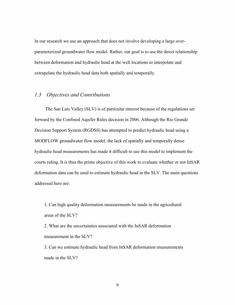
1.3 Objectives and Contributions

The San Luis Valley (SLV) is of particular interest because of the regulations set

forward by the Confined Aquifer Rules decision in 2006. Although the Rio Grande

Decision Support System (RGDSS) has attempted to predict hydraulic head using a

MODFLOW groundwater flow model, the lack of spatially and temporally dense

hydraulic head measurements has made it difficult to use this model to implement the

courts ruling. It is thus the prime objective of this work to evaluate whether or not InSAR

deformation data can be used to estimate hydraulic head in the SLV. The main questions

addressed here are:

1. Can high quality deformation measurements be made in the agricultural

areas of the SLV?

2. What are the uncertainties associated with the InSAR deformation

measurement in the SLV?

3. Can we estimate hydraulic head from InSAR deformation measurements

made in the SLV?

7

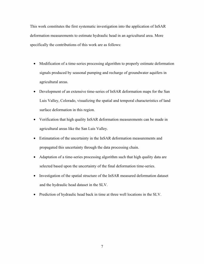
This work constitutes the first systematic investigation into the application of InSAR

deformation measurements to estimate hydraulic head in an agricultural area. More

specifically the contributions of this work are as follows:

• Modification of a time-series processing algorithm to properly estimate deformation

signals produced by seasonal pumping and recharge of groundwater aquifers in

agricultural areas.

• Development of an extensive time-series of InSAR deformation maps for the San

Luis Valley, Colorado, visualizing the spatial and temporal characteristics of land

surface deformation in this region.

• Verification that high quality InSAR deformation measurements can be made in

agricultural areas like the San Luis Valley.

• Estimatation of the uncertainty in the InSAR deformation measurements and

propagated this uncertainty through the data processing chain.

• Adaptation of a time-series processing algorithm such that high quality data are

selected based upon the uncertainty of the final deformation time-series.

• Investigation of the spatial structure of the InSAR measured deformation dataset

and the hydraulic head dataset in the SLV.

• Prediction of hydraulic head back in time at three well locations in the SLV.

8

Chapter 2

Theoretical Background

2.1 InSAR Background

In this section we outline the basics of Interferometric Synthetic Aperture Radar

(InSAR) processing, with specific reference to the measurement of deformation in the

San Luis Valley (SLV), Colorado. We begin by outlining the components of the

interferometric phase measurement and the InSAR processing flow. The different

components of the uncertainty in the deformation are outlined as the theoretical

background for Chapter 5. We end this section with an introduction to an advanced

processing technique known as Small Baseline Subset (SBAS) analysis, which we used to

process the data from the SLV.

2.1.1 InSAR imaging of deformation

Synthetic Aperture Radar (SAR) is a microwave imaging system, which uses a

radar antenna mounted on an airborne or satellite-based platform to transmit and receive

electromagnetic (EM) waves. The ERS-1 and ERS-2 satellites used in this study have a

11

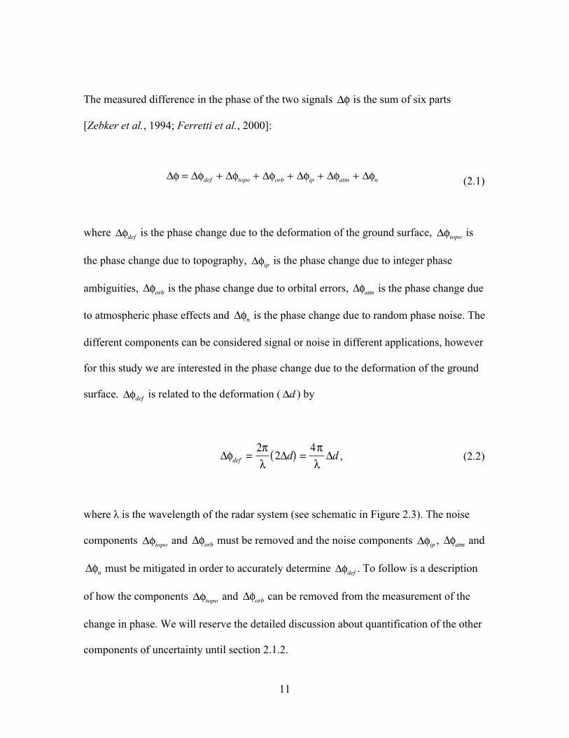
The measured difference in the phase of the two signals

�

Δφ is the sum of six parts

[Zebker et al., 1994; Ferretti et al., 2000]:

�

Δφ = Δφdef + Δφtopo + Δφorb + Δφip + Δφatm + Δφn (2.1)

where

�

Δφdef is the phase change due to the deformation of the ground surface,

�

Δφtopo is

the phase change due to topography,

�

Δφip is the phase change due to integer phase

ambiguities,

�

Δφorb is the phase change due to orbital errors,

�

Δφatm is the phase change due

to atmospheric phase effects and

�

Δφn is the phase change due to random phase noise. The

different components can be considered signal or noise in different applications, however

for this study we are interested in the phase change due to the deformation of the ground

surface.

�

Δφdef is related to the deformation (

�

Δd ) by

�

Δφdef =2πλ2Δd( ) =

4πλ

Δd , (2.2)

where λ is the wavelength of the radar system (see schematic in Figure 2.3). The noise

components

�

Δφtopo and

�

Δφorb must be removed and the noise components

�

Δφip ,

�

Δφatm and

�

Δφn must be mitigated in order to accurately determine

�

Δφdef . To follow is a description

of how the components

�

Δφtopo and

�

Δφorb can be removed from the measurement of the

change in phase. We will reserve the detailed discussion about quantification of the other

components of uncertainty until section 2.1.2.

14

result is geocoded, latitude and longitude co-ordinates are determined, so that the exact

location of the deformation at each pixel is known.

2.1.2 Uncertainty in the InSAR deformation measurement

Three major components remain and contribute to uncertainty in the measurement

of interferometric phase: integer phase ambiguities (

�

Δφ ip), atmospheric phase effects

(

�

Δφatm) and decorrelation of radar signals (

�

Δφn ). When we do not remove these

uncertainty components we can see in equation 2.3 that this uncertainty will propagate

through to an uncertainty in the InSAR deformation measurement:

�

Δd =λ4π

Δφ =λ4π

Δφdef + Δφip + Δφatm + Δφn( ). (2.3)

These components were discussed at length in Hanssen (2001). In Chapter 5 of this thesis

we will address two of these components: atmospheric phase effects and decorrelation of

radar signals, as we have found that these two components have the largest effect on the

uncertainty of the InSAR deformation measurement in the SLV. An outline of the theory

behind these two components is given in this section. The other component, integer phase

ambiguities, did not have a large effect on the uncertainty of the deformation in the SLV.

We will, however, discuss the theory behind this component in the paragraph to follow.

InSAR data processing includes a step called phase unwrapping, in which phases

measured modulo

�

2π are converted into a relative phase measurement by estimating and

15

adding the correct number of integer cycles of phase into the measurement. If there is a

considerable amount of noise in the data the algorithm will incorrectly estimate the phase

by some integer multiple of

�

2π , this is known as an integer phase ambiguity (

�

Δφip ). Usai

(2003) proposed a method for estimating this component of uncertainty by recognizing

the “closed-loop” condition of the change in phase in three interferograms:

�

φt1t2 + φt2t3 + φt3t1 = 0 , (2.4)

where

�

φti t j is the interferometric phase from scene i and scene j. However, using this

method with more interferograms is not simple and has not been attempted on datasets

with a large number of interferograms [Gonzalez and Fernandez, 2011]. As in Gonzalez

and Fernandez (2011), poor quality interferograms from the SLV were omitted, allowing

us to assume that this component of uncertainty is small.

If the atmospheric humidity, temperature, and pressure change significantly between the

two SAR scenes, the refractive index of the atmosphere will change. As the EM wave

passes through the atmosphere, the velocity of the EM wave will change and affect the

measured phase. The phase change due to atmospheric effects (

�

Δφatm ) is uncorrelated in

time, because the atmosphere changes randomly from one acquisition day to the next, but

correlated in space, because cloud cover, temperature, and pressure are continuous in

space over distances on the order of hundreds of meters [Hanssen, 1998; 2001]. For these

reasons it is common to use temporal and spatial filtering to remove this error component

[Zebker et al., 1997; Ferretti et al., 2001]. However, these atmospheric effects are highly

16

variable, often dominating the change in phase observed in interferograms. The limited

number of scenes used in any single analysis makes the associated uncertainty difficult to

quantify. Simons et al. (2002) estimated the uncertainty due to atmospheric phase effects

by looking at the root mean squared (RMS) difference between each interferogram and

all other interferograms in one data set. Because they knew that any surface deformation

in their study area was occurring slowly, they were able to attribute the RMS difference

to the uncertainty due solely to atmospheric phase effects. However, this method assumes

the same amount of uncertainty for every pixel in a given interferogram and does not

accurately represent the spatial variations in the uncertainty. Onn and Zebker (2006) used

Global Positioning System (GPS) estimates of water vapor to decrease the amount of

uncertainty in the InSAR deformation measurements, in some cases as much as 31%.

However, this analysis involves having a network of GPS measurements available, which

is not the case for many field sites.

A more recent study by Knospe and Jonsson (2010) investigated how atmospheric phase

effects vary spatially. In order to isolate the uncertainty due to atmospheric phase effects

they processed two interferograms that spanned a single day. They assumed that no

deformation was taking place over the time span of that day(

�

Δφdef = 0), and that

�

Δφ ip and

�

Δφn were also very small. This means that the measure phase change was all due to

changes in atmospheric conditions. They then created two variogram models that

quantified the spatial variability of the uncertainty. The variogram models were then used

to represent the uncertainty due to atmospheric phase effects for a synthetic data set. They

showed that the uncertainty in the final deformation estimates was less when the

17

variogram models were used to estimate the uncertainty due to atmospheric phase effects.

However, they stated that it is important to know which variogram model best represents

the uncertainty due to atmospheric phase effects for a given data set. Many applications

would not have a set of interferograms that span a single day, and hence would not

produce an appropriate variogram model of the uncertainty due to atmospheric phase

effects. In Chapter 5 we discuss how this component of uncertainty can be mitigated in

the data from the SLV.

The phase change due to phase noise (

�

Δφn) is caused by signal decorrelation and cannot

readily be compensated for without sacrificing spatial resolution. For a given pixel in an

interferogram the coherence is calculated as a quality measure for the phase difference

�

Δφn between two SAR scenes at that point. The complex coherence (γ) is defined as

follows:

(2.5)

where denotes the expected value, S1 and S2 are the complex values of SAR scene 1

and SAR scene 2, and and are the complex conjugates of SAR scene 1 and SAR

scene 2 for a small sample of pixels around the pixel in question. Often the magnitude of

the complex coherence is used, referred to as only the coherence, which can range from 0

to 1. An interferogram is described as coherent/well correlated, if many of the pixels have

coherence near 1; or as incoherent/decorrelated, if many of the pixels have coherence

near 0.

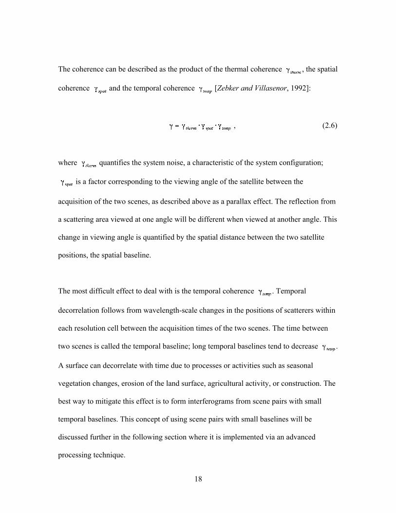
18

The coherence can be described as the product of the thermal coherence , the spatial

coherence and the temporal coherence [Zebker and Villasenor, 1992]:

, (2.6)

where quantifies the system noise, a characteristic of the system configuration;

is a factor corresponding to the viewing angle of the satellite between the

acquisition of the two scenes, as described above as a parallax effect. The reflection from

a scattering area viewed at one angle will be different when viewed at another angle. This

change in viewing angle is quantified by the spatial distance between the two satellite

positions, the spatial baseline.

The most difficult effect to deal with is the temporal coherence . Temporal

decorrelation follows from wavelength-scale changes in the positions of scatterers within

each resolution cell between the acquisition times of the two scenes. The time between

two scenes is called the temporal baseline; long temporal baselines tend to decrease .

A surface can decorrelate with time due to processes or activities such as seasonal

vegetation changes, erosion of the land surface, agricultural activity, or construction. The

best way to mitigate this effect is to form interferograms from scene pairs with small

temporal baselines. This concept of using scene pairs with small baselines will be

discussed further in the following section where it is implemented via an advanced

processing technique.

19

2.1.3 Small Baseline Subset (SBAS) analysis

The SLV is an agricultural area where crop growth, irrigation, land erosion and

harvesting cycles can all change the height of the imaged surface between the acquisition

of any two SAR scenes, leading to decorrelation of the signals. A recently developed

technique, small baseline subset (SBAS) analysis, combines the coherent areas in a series

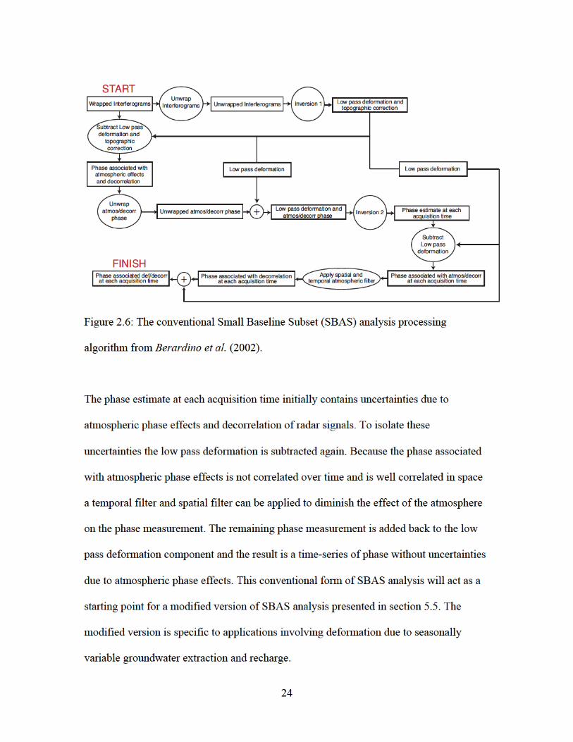
of interferograms to produce a map of deformation time-series [Berardino et al., 2002].

Phase decorrelation is minimized by imposing constraints on the temporal and spatial

baselines for each pair of scenes that are interfered.

The basic principle underlying SBAS is proper interferogram selection combined with a

least squares (LS) analysis of the phases in the resulting unwrapped interferograms.

Interferogram selection is illustrated in Figure 2.5, a plot of spatial versus temporal

baseline for all available SAR scenes from an area. Each scene is shown as a circle with

the spatial and temporal baselines plotted relative to the first scene. Lines, which signify

an interferogram, connect scenes if the spatial and temporal baselines are below some

selected threshold. In general, a smaller spatial baseline leads to better coherence,

therefore the goal is to minimize the spatial baseline threshold for the set of

interferograms. The temporal baseline threshold is dependent on how rapidly the height

of the vegetation changes with time in a given area and so, for example, could be 6 years

for areas in an arid climate, but a few months for vegetated areas. Each group of

connected scenes is known as a small baseline subset. As long as the subsets overlap for

some period of time, a singular value decomposition (SVD) can be used to solve for a

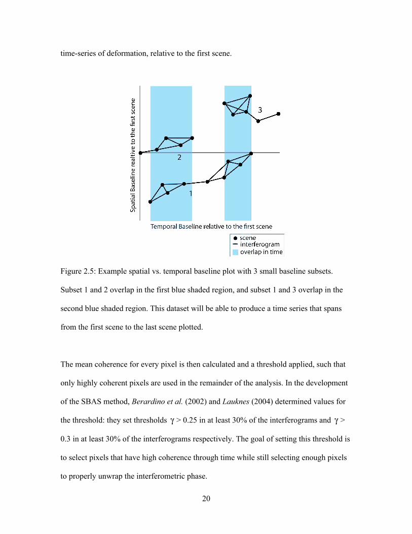
20

time-series of deformation, relative to the first scene.

Figure 2.5: Example spatial vs. temporal baseline plot with 3 small baseline subsets.

Subset 1 and 2 overlap in the first blue shaded region, and subset 1 and 3 overlap in the

second blue shaded region. This dataset will be able to produce a time series that spans

from the first scene to the last scene plotted.

The mean coherence for every pixel is then calculated and a threshold applied, such that

only highly coherent pixels are used in the remainder of the analysis. In the development

of the SBAS method, Berardino et al. (2002) and Lauknes (2004) determined values for

the threshold: they set thresholds

�

γ > 0.25 in at least 30% of the interferograms and

�

γ >

0.3 in at least 30% of the interferograms respectively. The goal of setting this threshold is

to select pixels that have high coherence through time while still selecting enough pixels

to properly unwrap the interferometric phase.

21

We will now review the mathematical formulation from Berardino et al. (2002) that

describes the SBAS technique as performed on the selected pixels. Let us consider N + 1

SAR scenes acquired at times (t0, t1,…, tN). Each scene must be able to interfere with one

other scene, so the minimum number for each subset is two scenes. If N is odd, the

number of different interferograms M is given by:

. (2.7)

If we consider the jth interferogram made with SAR scenes at tA and tB we can define the

change in phase measured at each pixel position in terms of range direction and azimuth

direction (x,r) as follows:

�

ΔΦ(x,r) = Φ(tB ,x,r)− Φ(tA,x,r)

≈ 4πλ

d(tB ,x,r)− d(tA,x,r)[ ], (2.8)

where d(tB,x,r) is the deformation at time tB relative to zero deformation at time t0 and

d(tA,x,r) is the deformation at time tA relative to zero deformation at time t0. If we look at

all deformation relative to the time t0 then the phase time series becomes

�

Φ(ti ,x,r) ≈ 4πd(ti ,x,r)/λ, for i = 1,…, N. For this initial description of the analysis we

ignore all phase change due to atmospheric effects, topographic effects and phase noise,

22

as our goal in processing is to remove all components of the signal not related to the

deformation. We also assume that the phase for each pixel is properly unwrapped. For the

remainder of the solution we will look at the deformation time series for one pixel, so the

(x,r) dependence drops out.

We have N unknowns for the phase which are needed to compute deformation relative to

t0:

�

ΦT = Φ(t1),...,Φ(tN )[ ] (2.9)

and we have M data points from the computed interferograms:

�

ΔΦT = ΔΦ1,...,ΔΦM[ ]. (2.10)

We relate our data to our unknowns with M equations as follows:

�

ΔΦ j = Φ(tBj)− Φ(tAj

) j = 1,...,M (2.11)

where

�

Φ(tAj ) is the phase at the time of scene A and

�

Φ(tBj ) is the phase at the time of

scene B. This gives us a system of M equations and N unknowns with the matrix

representation:

�

AΦ = ΔΦ. (2.12)

23

The matrix

�

A outlines the set of interferograms from the available data. We can solve for

�

Φ in equation 2.11 by inverting the matrix

�

A , i.e. performing a SVD of

�

A . The

formulation given with equations 2.7 – 2.12 is the basic least squares inversion problem.

In practice there are other steps that account for prior information about the type of

deformation, the topographic correction, and atmospheric effects. For thoroughness we

outline the steps of what we call ‘conventional SBAS analysis’, which is based upon the

processing flow described in Berardino et al. (2002).

The processing flow for conventional SBAS analysis is shown in Figure 2.6. Square

boxes are used to define objects and circles to define actions performed on those objects.

In Berardino et al. (2002) prior information about the deformation is used to define a

low-pass deformation model that can capture the low frequency component of the

deformation. This model is often chosen to be a simple linear, quadratic or sine function.

The authors start by unwrapping the interferometric phases and then apply ‘Inversion 1’,

shown in Figure 2.6. ‘Inversion 1’ estimates the parameters of the low-pass deformation

model and the topographic correction. The phase associated with these two components is

then subtracted from the wrapped interferometric phases. The remaining phase is

associated with atmospheric phase effects and decorrelation. This phase is unwrapped

and then added back to the phase associated with the low pass deformation model. On

these data ‘Inversion 2’ is applied, yielding a phase estimate at each acquisition time.

25

2.2 Aquifer deformation background

In this section we outline the basics of aquifer deformation theory. We begin by

reviewing the analytical equations that relate changes in hydraulic head in confined

aquifer systems to aquifer system deformation. We finish this section with a short review

of coupled hydromechanical systems that will be considered at the field site in the San

Luis Valley (SLV), Colorado.

2.2.1 Theoretical definitions

An aquifer is a geologic system, often taking the form of a permeable sedimentary

unit, from which economical amounts of water can be pumped. Aquifers can be

unconfined, if the system is exposed to atmospheric pressure, or confined, if the system is

kept at a pressure higher than atmospheric. Aquitards or confining layers are low

permeability layers that confine fluid pressures in the underlying confined aquifers. The

low permeability material of the confining layer is generally clay or silt. We review

below a summary of aquifer deformation theory as it applies to InSAR deformation data

[Hoffmann, 2003].

The theory of aquifer deformation was first formalized in terms of Terzaghi’s theory of

poroelasticity [Terzaghi, 1925]:

(2.13)

26

where the , effective stress, is equal to , the total stress on the aquifer system, minus

�

p, the pore pressure. One can express a change in pore pressure,

�

Δp, as a change in

hydraulic head, , which can be measured from wells that are sampling the aquifer

system [Fetter, 2001]:

(2.14)

where is acceleration due to gravity and ρ is the density of water. In confined aquifer

systems one assumes that the total stress does not change (

�

Δσ = 0 ), i.e. the stress induced

by the overburden is not changing. However, stress change occurs as water is withdrawn

from the pore space (

�

−Δh ). The decrease in pore water pressure results in an effective

stress increase (

�

Δ ′ σ ), which is born by the aquifer system skeleton

. (2.15)

It is the change in effective stress that causes the deformation of sediments.

Terzaghi’s theory was expanded upon by Biot (1941) to investigate the effects of 3D

deformation. If the following assumptions are made: a) down into Earth is one of the

principle stress directions and b) the lateral extent of the aquifer is much greater than the

vertical extent, then only the vertical portion of the effective stress ( ) is relevant. The

partial differential equation that results from combining Darcy’s Law for fluid flow with

the continuity equation is known as the one dimensional diffusion equation:

27

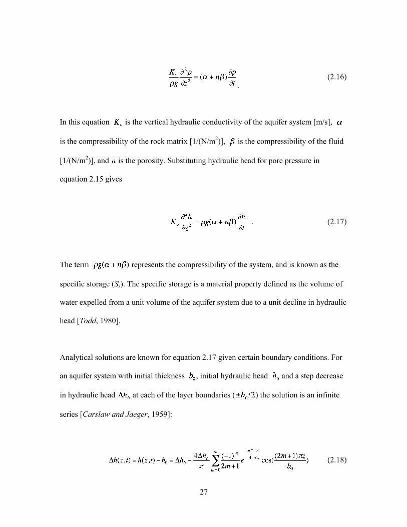
. (2.16)

In this equation is the vertical hydraulic conductivity of the aquifer system [m/s],

is the compressibility of the rock matrix [1/(N/m2)], is the compressibility of the fluid

[1/(N/m2)], and is the porosity. Substituting hydraulic head for pore pressure in

equation 2.15 gives

. (2.17)

The term represents the compressibility of the system, and is known as the

specific storage (Ss). The specific storage is a material property defined as the volume of

water expelled from a unit volume of the aquifer system due to a unit decline in hydraulic

head [Todd, 1980].

Analytical solutions are known for equation 2.17 given certain boundary conditions. For

an aquifer system with initial thickness , initial hydraulic head and a step decrease

in hydraulic head at each of the layer boundaries ( ) the solution is an infinite

series [Carslaw and Jaeger, 1959]:

(2.18)

28

where .

All of the terms in this series are not necessary to get a good estimate of the change in

hydraulic head as a function of depth and time. A value of particular interest is the time

constant associated with the first term in the series;

�

τ(m=0) = τ0 .

�

τ0 is the deformation time

constant and represents the time after which the hydraulic head in the layer is 93%

equilibrated with the boundary conditions [Scott, 1963; Riley, 1969].

Given this solution of the flow equation the link can be made between the change in

hydraulic head and the change in aquifer thickness. In a confined aquifer system water is

derived both from reduction of pore space ( ) and expansion of the pore water ( ).

(2.19)

where Ssk is the skeletal specific storage and Ssw is the specific storage of water. Ssk is

responsible for most of the water production as it is generally two to three orders of

magnitude larger than Ssw (water is essentially an incompressible fluid).

We now show the derivation of the analytical solution for the equivalent change in

aquifer thickness caused by a symmetric decrease in hydraulic head. The definition of

according to Fetter (2001) is:

29

(2.20)

where is the change in total volume (thickness) and is the original total volume.

Looking at only the vertical displacements:

(2.21)

where is the change in thickness of a given volume and is the rock matrix

compressibility in the vertical direction. Substituting the change in effective stress in the

vertical direction, from equation 2.13 into equation 2.19 gives:

. (2.22)

We rearrange equation 2.22 and substitute the relation for Ssk from equation 2.19 to get

�

Sskb0 = ΔbΔh

. (2.23)

30

The skeletal storage coefficient is a new parameter equal to the product of the

compressibility of the aquifer system and the initial thickness of the aquifer system,

. Defining things in this way shows that, for a given aquifer system, there is a

linear relationship between the change in thickness and the change in stress of a given

unit that is governed by the skeletal storage coefficient.

We next substitute

�

Δh from equation 2.18 into equation 2.23 and calculate the integral

over the total height of the aquifer system. The thickness changes as a function of time as

follows

. (2.24)

This equation is not entirely applicable to real aquifer systems as time variant boundary

conditions complicate this simple solution. However, it is possible now to identify the

approximately linear relationship between hydraulic head and aquifer system compaction.

Up until now the discussion has involved lumped aquifer and aquitard properties for any

aquifer system. However, the two types of hydrogeologic units, aquifers and aquitards,

deform in one of two ways: ‘elastically’ or ‘inelastically’, depending on the stress history

and the current state of stress. Poland et al. (1975) describe the difference between elastic

and inelastic deformation as follows. Aquifers deform primarily elastically at the depths

of typical groundwater production. However, aquitards require two skeletal storage terms

31

�

Ssk =Sske → ′ σ z < ′ σ z(max)Sskv → ′ σ z ≥ ′ σ z(max)

⎧ ⎨ ⎩

. (2.25)

If the effective stress is less than any previously experienced effective stress, known as

the maximum effective stress ( ), then the aquitards will deform elastically and all

deformation is recoverable. However, if is exceeded the aquitards will begin to

deform inelastically and there will be permanent non-recoverable deformation. Often

is referred to as a minimum preconsolidation head ( ). In many cases linearizing

equation 2.24 can approximate elastic deformation

. (2.26)

Lab tests have shown that the relation for inelastic deformation in fine-grained sediments

is approximately logarithmic [Jorgensen, 1980]. If, however, the changes in effective

stress are small,

�

Δh less than 100 m, then a linear equation arises as well [Leake and

Prudic, 1991]:

. (2.27)

It is important to remember that in equations 2.26 and 2.27 we assume that the head

throughout the layer has equilibrated with the hydraulic head at the boundaries. The time

scale for this realization is which, from equation 2.18, is proportional to the skeletal

storage term. Because values of are generally ten to one hundred times larger than

32

values of , the time constant for elastic deformation is on the order of days while the

time constant for inelastic deformation can be on the order of years or decades [Ireland et

al., 1984; Riley, 1998]. For a typical aggregate thickness of an aquifer system, of the

aquitards is so large that it can be assumed to represent the inelastic storage coefficient

for the entire aquifer system [Poland et al., 1975].

The analytical solution for the 1-D diffusion equation discussed above shows that there is

a time scale for equilibrating the hydraulic head throughout a layered aquifer system.

This time scale will vary based on stress conditions and aquifer material properties. In the

next section we will discuss how this theory may be applied to a complex aquifer system

like the SLV.

2.2.2 Coupled hydromechanical systems

The assumptions made during the analytical formulation of equation 2.26 may not

be valid for the hydro-mechanical model that has been created for the SLV. In general it

is not true that a symmetric change in head occurs at each boundary of the aquifer system

(see assumptions for solution of equation 2.17). Figure 2.7 is a simple sketch of the

movement of water in a valley type confined aquifer system. The confined aquifer system

is kept under pressure by an aquitard or confining layer, and recharged from the edges of

the valley floor by water runoff. This stored water is then extracted from irrigation wells

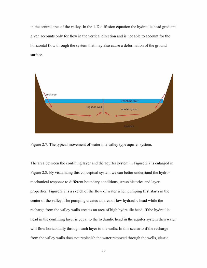
33

in the central area of the valley. In the 1-D diffusion equation the hydraulic head gradient

given accounts only for flow in the vertical direction and is not able to account for the

horizontal flow through the system that may also cause a deformation of the ground

surface.

Figure 2.7: The typical movement of water in a valley type aquifer system.

The area between the confining layer and the aquifer system in Figure 2.7 is enlarged in

Figure 2.8. By visualizing this conceptual system we can better understand the hydro-

mechanical response to different boundary conditions, stress histories and layer

properties. Figure 2.8 is a sketch of the flow of water when pumping first starts in the

center of the valley. The pumping creates an area of low hydraulic head while the

recharge from the valley walls creates an area of high hydraulic head. If the hydraulic

head in the confining layer is equal to the hydraulic head in the aquifer system then water

will flow horizontally through each layer to the wells. In this scenario if the recharge

from the valley walls does not replenish the water removed through the wells, elastic

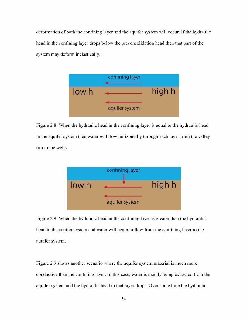
34

deformation of both the confining layer and the aquifer system will occur. If the hydraulic

head in the confining layer drops below the preconsolidation head then that part of the

system may deform inelastically.

Figure 2.8: When the hydraulic head in the confining layer is equal to the hydraulic head

in the aquifer system then water will flow horizontally through each layer from the valley

rim to the wells.

Figure 2.9: When the hydraulic head in the confining layer is greater than the hydraulic

head in the aquifer system and water will begin to flow from the confining layer to the

aquifer system.

Figure 2.9 shows another scenario where the aquifer system material is much more

conductive than the confining layer. In this case, water is mainly being extracted from the

aquifer system and the hydraulic head in that layer drops. Over some time the hydraulic

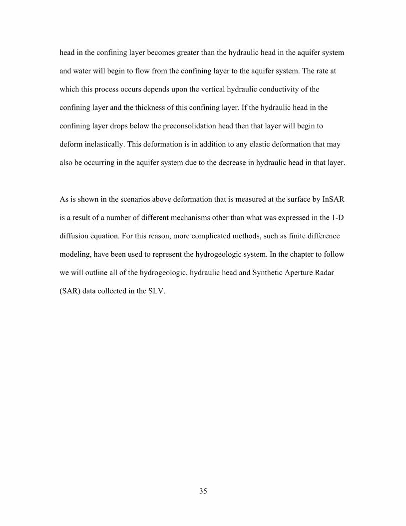
35

head in the confining layer becomes greater than the hydraulic head in the aquifer system

and water will begin to flow from the confining layer to the aquifer system. The rate at

which this process occurs depends upon the vertical hydraulic conductivity of the

confining layer and the thickness of this confining layer. If the hydraulic head in the

confining layer drops below the preconsolidation head then that layer will begin to

deform inelastically. This deformation is in addition to any elastic deformation that may

also be occurring in the aquifer system due to the decrease in hydraulic head in that layer.

As is shown in the scenarios above deformation that is measured at the surface by InSAR

is a result of a number of different mechanisms other than what was expressed in the 1-D

diffusion equation. For this reason, more complicated methods, such as finite difference

modeling, have been used to represent the hydrogeologic system. In the chapter to follow

we will outline all of the hydrogeologic, hydraulic head and Synthetic Aperture Radar

(SAR) data collected in the SLV.

36

Chapter 3

Overview of available data

There are two main goals for this chapter: 1) to introduce the field site, 2) to outline

all of the available data in the San Luis Valley (SLV). We will first discuss the

geographic regions of the SLV, which will become pertinent when we introduce the

complex hydrogeology. We will summarize the work of the Rio Grande Decision Support

System (RGDSS) to build hydrogeologic layer maps and parameter zones for aquifer

properties. Then we will introduce the Synthetic Aperture Radar (SAR) and hydraulic

head data.

3.1 Introduction to the field site

The San Luis Valley (SLV) is a rift valley in south-central Colorado bounded by

igneous, metamorphic, and sedimentary bedrock of the Sangre de Cristo and San Juan

mountain ranges. The basin has a graben structure, known as the Baca graben, and

contains valley fill that consists of interbedded deposits of sand, clay, gravel, and some

37

layers of volcanic rocks [Hearne and Dewey, 1988]. The boundary of the SLV is defined

by the extent of the sediments that fill the San Luis Basin which extends down into New

Mexico [Emery et al., 1973].

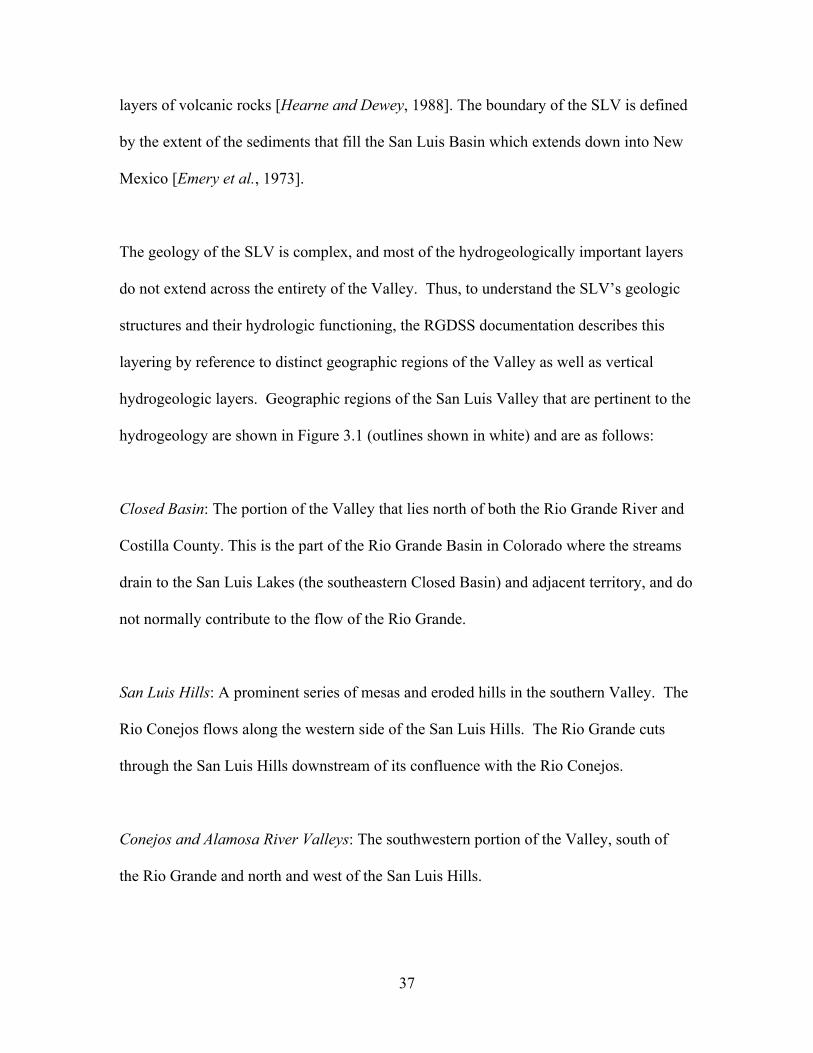
The geology of the SLV is complex, and most of the hydrogeologically important layers

do not extend across the entirety of the Valley. Thus, to understand the SLV’s geologic

structures and their hydrologic functioning, the RGDSS documentation describes this

layering by reference to distinct geographic regions of the Valley as well as vertical

hydrogeologic layers. Geographic regions of the San Luis Valley that are pertinent to the

hydrogeology are shown in Figure 3.1 (outlines shown in white) and are as follows:

Closed Basin: The portion of the Valley that lies north of both the Rio Grande River and

Costilla County. This is the part of the Rio Grande Basin in Colorado where the streams

drain to the San Luis Lakes (the southeastern Closed Basin) and adjacent territory, and do

not normally contribute to the flow of the Rio Grande.

San Luis Hills: A prominent series of mesas and eroded hills in the southern Valley. The

Rio Conejos flows along the western side of the San Luis Hills. The Rio Grande cuts

through the San Luis Hills downstream of its confluence with the Rio Conejos.

Conejos and Alamosa River Valleys: The southwestern portion of the Valley, south of

the Rio Grande and north and west of the San Luis Hills.

40

confined aquifer system (layers 3 – 5). They determined the relative thickness of the

layers by creating a database of driller’s logs. The lithologic data came from three

sources: the RGDSS piezometer logs, the State Engineer’s Office (SOE) reports and

various geophysical logs. The Department of Defense Groundwater Modeling System

(GMS) was used to interpolate between the various lithologic data using a kriging

method.

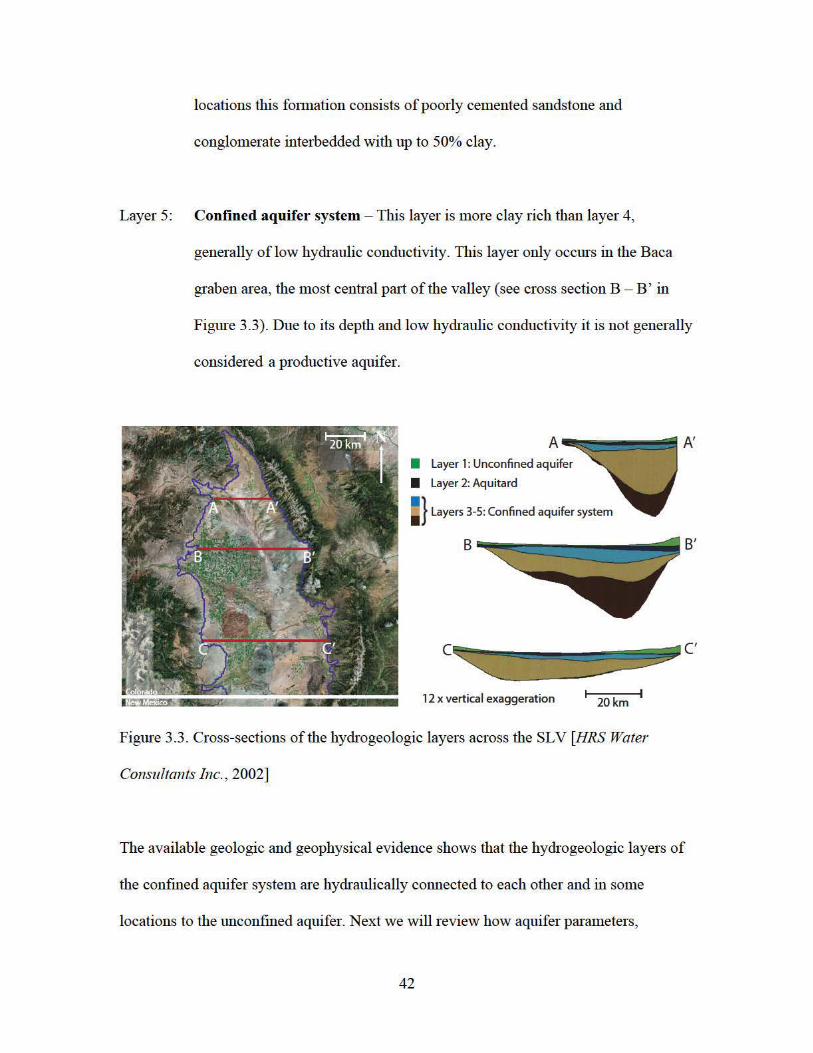
Three cross sections of the hydrogeologic layers are given in Figure 3.3. We can see that

the thickness of the layers varies significantly from north to south in the valley. It is

important to note that the lithology of these layers also varies from north to south. Below

we provide a generalized geologic description of the layers (beginning with the top

layer):

Layer 1: Unconfined aquifer – This layer contains mainly sand, gravel, and cobbles,

with minor thin (<10 ft.) clay units. The layer thickness ranges from 15 to 150

m.

Layer 2: Aquitard – This layer contains lacustrine sediments, clay dominated with

generally less than 25% sand or gravel content. It is known as the ‘blue clay’

layer in some areas of the valley and in other areas it appears as unfractured

volcanic rocks [Emery et al., 1973; Hearne and Dewey, 1988]. Considered as

a whole this layer acts as an aquitard to confine deeper layers. However, the

sand layers within this clay-dominated series do still constitute an aquifer in

41

some parts of the SLV. This layer is over 120 m thick in the center of the

Closed Basin and 1 m thick near the edges of the valley (see cross section B –

B’ in Figure 3.3). In Costilla County this layer does not exist, rather a series

of discontinuous clay and sand layers act as the aquitard (see cross section C

– C’ in Figure 3.3).

Layer 3: Confined aquifer system – In the northern portion of the SLV this layer

contains mainly sand, although clay layers do still appear. Sand or sandstone

layers make up at least 50% of the interval (see Figure 3.2). This is generally

interpreted to be the most productive portion of the confined aquifer system.

In the southern portion of the SLV layer 3 is composed of the Hinsdale and

Servilleta Basalts (see Figure 3.2). In the Conejos and Alamosa River valleys

it is interbedded with the Hinsdale Formation basalt lava flows. In Costilla

County this layer contains the Servilleta Formation, consisting primarily of

basalt lava flows located south of the San Luis Hills. These lava-flow layers

vary from thin and highly fractured to very thick and unfractured. The thick

and unfractured lava flows form a confining layer or aquitard. In some areas

the permeability is very high, and hence this layer is considered a productive

portion of the confined aquifer system.

Layer 4: Confined aquifer system – This layer is predominantly sand and gravel with

up to 50% clay in most areas of the SLV. In Costilla County, this layer also

contains volcanic/volcaniclastic rocks. Evidence indicates that in some

43

collected by performing aquifer tests, were assigned to the different hydrogeologic layers.

3.2.2 Aquifer parameters

There were 148 and 151 aquifer tests for the unconfined aquifer and the confined

aquifer system respectively. Estimates of aquifer parameters were made by performing

aquifer tests and using traditional curve-matching methods of data analysis [Harmon,

2001]. These parameters were then assigned to the hydrogeologic layers described in the

previous section. Because the hydrogeology in the SLV is so variable from north to south

and east to west, HRS Water Consultants created parameter zones that honor these

changes in the horizontal plane. The estimates of aquifer parameters were then parsed

directly into these different zones.

An aquifer test involves pumping water out of the aquifer system at a pumping well and

inducing a drawdown of the hydraulic head at monitoring wells some distance away. The

well that the water is pumped from is referred to as the aquifer test well. Once pumping is

finished the hydraulic head levels rebound. During this rebound the hydraulic head

change through time is measured at the aquifer test well. This measurement is compared

to an analytical solution of the hydraulic head change (e.g. Theis equation or Hantush-

Jacob formula). The transmissivity (T) and the storage coefficient (S) are the estimated

aquifer parameters that allow the analytical solution to match the measurements. For an

accurate measure of S at least one other well must be monitored other than the aquifer test

well.

44

The estimated aquifer test parameters were assigned to the hydrogeologic layers based on

the interval of the aquifer system screened at the aquifer test well. Once all the aquifer

parameters were assigned to a hydrogeologic layer they were distributed the horizontal

place by interpolating, through kriging, the estimated parameters within a parameter

zone. The combined use of kriging with parameter zones ensures the exact value of the

aquifer parameter is honored at the measurement location, while maintaining the general

distribution of geologic materials.

3.3 Hydraulic head

Hydraulic head measurements in the SLV are either made in open wells or using

piezometers. For most open wells the well casing is effectively attached to the aquifer

material for the entire screened interval. The casing has a part that extends beyond the

height of the ground surface, this is known as the 'stickup'. The depth to water (DTW) is

measured from the stickup to the water level in the well. That value is then referenced to

the height of the ground surface, which has been surveyed or taken from a topographic

map. If the height of the ground surface is taken from a topographic map then it is

generally known to within a foot.

Each RGDSS piezometer has a 4-inch diameter screened interval where gravel was

packed in the annulus between screen and borehole. The intervening 4-inch diameter

casing intervals were filled with Portland cement. Above the uppermost screened interval

the annulus between casing and borehole was filled with Portland cement. The casing and

screen are locked into place along the entire length of the piezometer by the friction

45

between borehole and gravel pack (or Portland cement), and by the friction between

casing/screen and cement or gravel pack. It is expected that the casing expands and

contracts synchronously with the compression and rarefaction of the aquifer/aquitard. The

hydraulic heads at the piezometer locations are also measured against a stickup and

referenced to the height of the ground surface.

The RGDSS database contains information about the well network with tables that are

linked to the location, position of the screened interval and the ground level elevation of

each well. There are over 1200 wells in the SLV, but at only 328 wells are there hydraulic

head measurements in the confined aquifer system. In the chapter to follow we will

review the hydraulic head data to determine which of the 328 wells can be used in

conjunction with the InSAR deformation data.

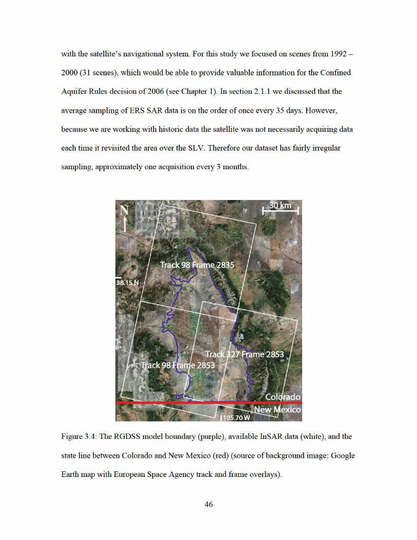
3.4 Synthetic Aperture Radar (SAR) data

SAR data for the SLV were acquired from two sources: the Western North

American Interferometric Synthetic Aperture Radar Consortium (WInSAR) and the

European Space Agency (ESA). In this study data from the ERS-1 and ERS-2 satellites

were used, covering the period from 1992 to 2000. Figure 3.4 shows the RGDSS model

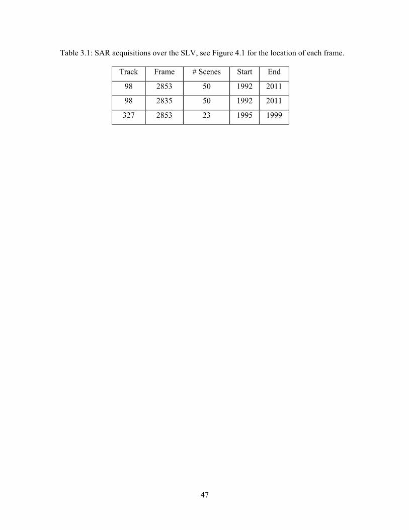
boundary and the spatial extent of available scenes. Table 3.1 shows the number of

scenes that were acquired over the SLV.

This study focused on track 98 and frame 2853, which has 50 scenes with good spatial

coverage of the valley. Scenes from 2001-2005 could not be used because of problems

47

Table 3.1: SAR acquisitions over the SLV, see Figure 4.1 for the location of each frame.

Track Frame # Scenes Start End

98 2853 50 1992 2011

98 2835 50 1992 2011

327 2853 23 1995 1999

48

Chapter 4

Assessment of hydraulic head data

In this chapter we will first investigate the spatial and temporal sampling of the

hydraulic head data at wells in the confined aquifer system (see section 4.1). Next we

need to ensure that the amount of deformation caused by changes in hydraulic head in the

San Luis Valley can accurately be measured using InSAR. We calculate the average

seasonal hydraulic head change at each well location and use estimates of Ske to predict

the amount of deformation we expect to see at the surface (see section 4.2).

4.1 Review of hydraulic head data

Of the 328 wells sampling the confined aquifer system only 69 wells had

hydraulic head measurements from 1992 – 2000 (time span of InSAR data) and were

located within the SAR scene (track 98 frame 2853 introduced section 3.4). An initial

assessment of the data found that 19 wells had ≤ 2 hydraulic head measurements from

1992 – 2000. Because of the low temporal sampling at these 19 well locations the

49

hydraulic head data were not used for further analysis. In the sections to follow we

discuss the spatial and temporal sampling of the hydraulic head data at the remaining 50

wells.

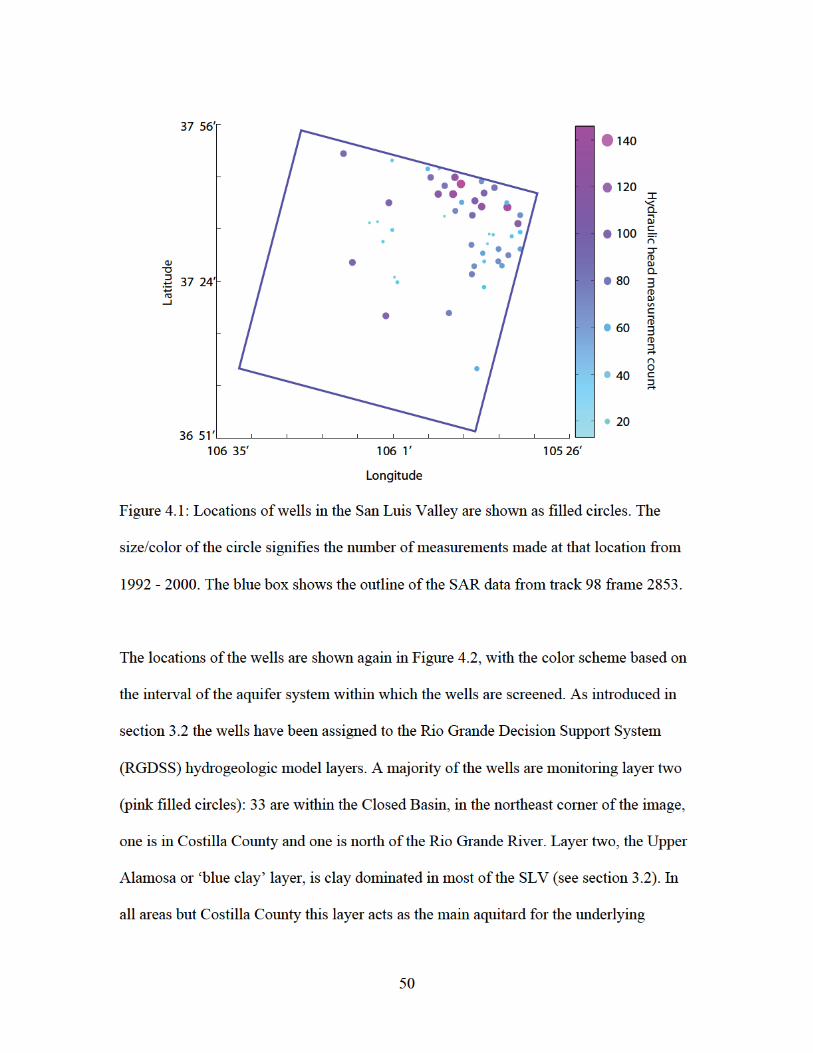
4.1.1 Spatial sampling of hydraulic head data

The locations of the 50 wells are shown as filled circles in Figure 4.1, with the

outline of track 98 frame 2853 shown as a blue box. The size/color of the circle signifies

the number of hydraulic head measurements made at that location. A majority of the

wells (33) are located within the Closed Basin area of the SLV (northeast corner of the

Figure 4.1).

An important piece of information about the hydraulic head data that is relevant for our

study is that the wells are monitoring specific intervals of the groundwater system, while

the deformation measured by InSAR is for the entire system. Therefore, an important step

in any analysis of InSAR deformation and hydraulic head should be to determine the

hydrogeologic interval the wells are monitoring. In the SLV information on well

construction, which would provide the depth and extent of the screened interval, was not

collected for all wells. Most of the wells in the SLV were initially drilled to extract water

at a high flow rate. It is common that once the drillers encounter a high flowing interval

drilling is stopped [Willem Schreuder personal communication, 2011]. Consequently, we

assume that the lowest unit in the well is the interval of the aquifer being monitored.

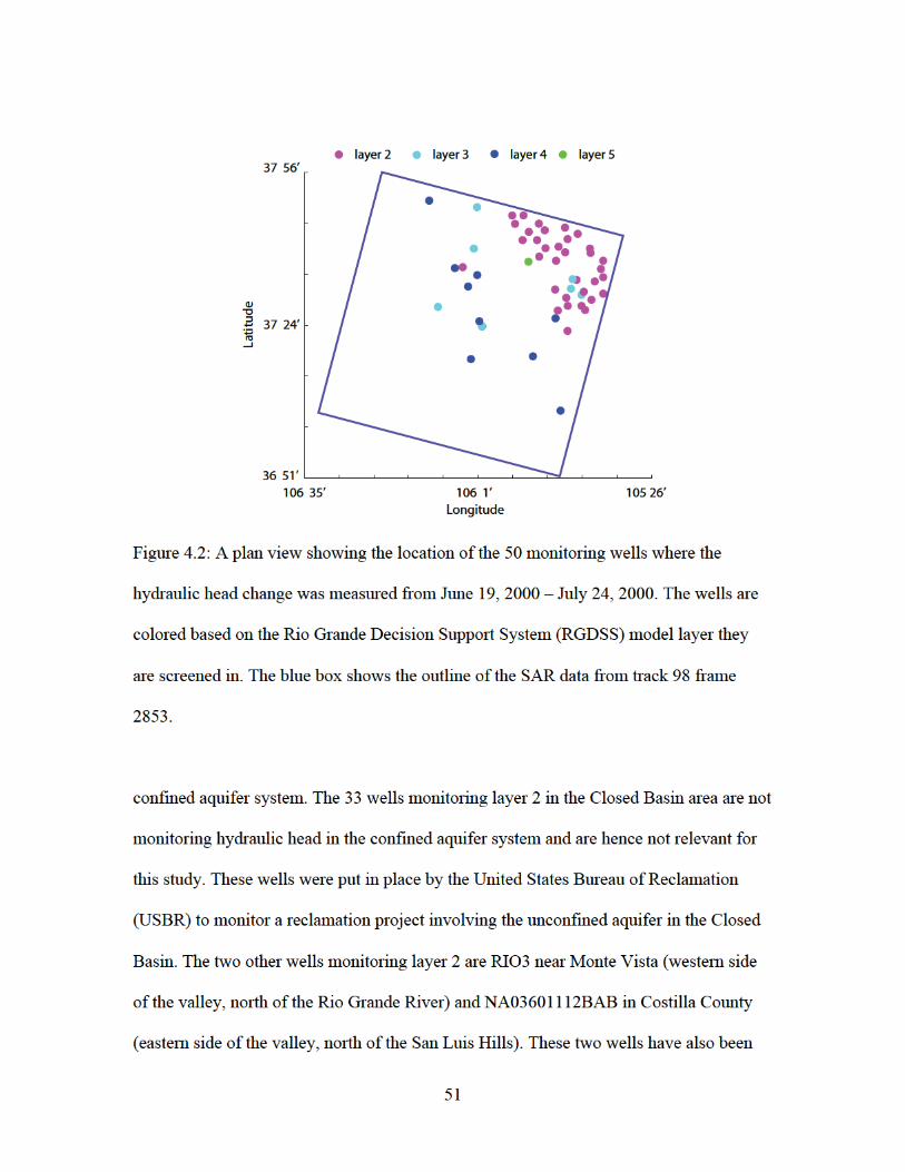
52

removed from the analysis to follow as they may be in areas where layer 2 is still the

confining unit (see section 3.2 for more information on the continuity of the confining

unit in the SLV). The remaining 15 wells were used for further analysis in this chapter.

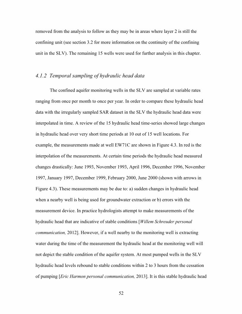
4.1.2 Temporal sampling of hydraulic head data

The confined aquifer monitoring wells in the SLV are sampled at variable rates

ranging from once per month to once per year. In order to compare these hydraulic head

data with the irregularly sampled SAR dataset in the SLV the hydraulic head data were

interpolated in time. A review of the 15 hydraulic head time-series showed large changes

in hydraulic head over very short time periods at 10 out of 15 well locations. For

example, the measurements made at well EW71C are shown in Figure 4.3. In red is the

interpolation of the measurements. At certain time periods the hydraulic head measured

changes drastically: June 1993, November 1993, April 1996, December 1996, November

1997, January 1997, December 1999, February 2000, June 2000 (shown with arrows in

Figure 4.3). These measurements may be due to: a) sudden changes in hydraulic head

when a nearby well is being used for groundwater extraction or b) errors with the

measurement device. In practice hydrologists attempt to make measurements of the

hydraulic head that are indicative of stable conditions [Willem Schreuder personal

communication, 2012]. However, if a well nearby to the monitoring well is extracting

water during the time of the measurement the hydraulic head at the monitoring well will

not depict the stable condition of the aquifer system. At most pumped wells in the SLV

hydraulic head levels rebound to stable conditions within 2 to 3 hours from the cessation

of pumping [Eric Harmon personal communication, 2013]. It is this stable hydraulic head

53

that the RGDSS model aims to model, and hence we must evaluate to what extent InSAR

deformation data can inform these measurements.

To remove the effects of these rapid perturbations in the hydraulic head time-series (blue

markers are highlighted with arrows in Figure 4.3) a moving window average was

applied to the interpolated data. The window length of the temporal filter was varied until

an optimal value was found. A window length of 90 days allowed for the mitigation of

these rapid perturbations without removing the entirety of the seasonal groundwater

signal (see the green dashed line in Figure 4.3). The same moving window average was

applied to the hydraulic head data from all 15 wells.

Figure 4.3: Hydraulic head measured at well EW71C shown with blue markers. The

arrows signify hydraulic head measurements that may be affected by instrument errors or

pumping at nearby wells.

Jun92 Jun93 Jun94 Jun95 Jun96 Jun97 Jun98 Jun99 Jun00!16

!14

!12

!10

!8

!6

!4

!2

Hyd

raul

ic h

ead

(ft)

measurementsinterpolatedinterpolated with moving window

54

4.2 Predicted deformation

The goal for this section is to predict the seasonal magnitude of the deformation

that we expect to see at each of the remaining 15 well locations (shown in Figure 4.4). In

order to do so we first assume that the deformation occurring in the SLV is elastic. This

allows us to rearrange equation 2.26 as follows:

(4.1)

where Δd is the predicted deformation at the surface, Sske is the skeletal elastic storage

coefficient, b* is the thickness of the producing aquifer unit, and Δh is the change in

hydraulic head. We can see that if the product of Sske, b* and Δh is small the deformation

at the surface will not be large enough to be accurately measured using InSAR. For this

analysis we will assume that the uncertainty in the InSAR measurement is approximately

5 mm [Hoffman et al., 2002]. This means that predicted deformations of less that 1 cm

will not be accurately determined by InSAR.

In order to simplify the analysis we created an aggregate variable, seasonal hydraulic

head change (Δhs), which is the average seasonal peak-to-trough change in hydraulic

head. We used upper and lower bounds for Sske from the literature (see Table 4.1). Where

the producing lithology was not known we used the Sske values for sand, as it is most

likely that an aquifer is producing water from a sandy lithologic unit in the San Luis

Valley. We note that there are cases for solid rock where Sske can be less than 3.3E-6, but

for the analysis given below we will only consider the fissured/jointed rock case. Most of

€

Δd = Sskeb*Δh

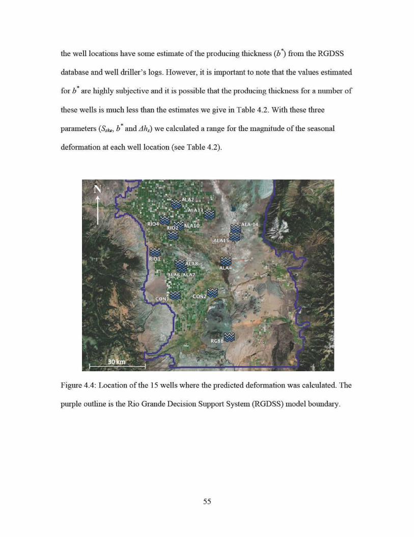
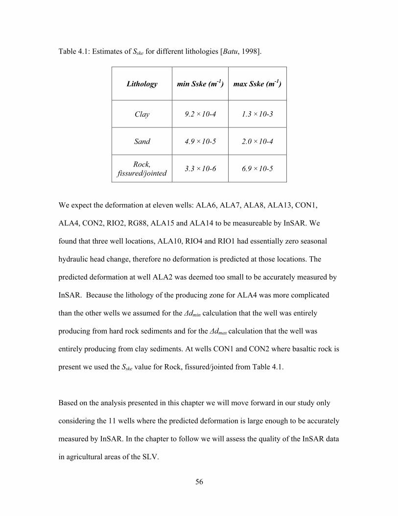
56

Table 4.1: Estimates of Sske for different lithologies [Batu, 1998].

Lithology min Sske (m-1)

max Sske (m-1)

Clay

9.2 ×10-4

1.3 ×10-3

Sand 4.9 ×10-5

2.0 ×10-4

Rock, fissured/jointed

3.3 ×10-6

6.9 ×10-5

We expect the deformation at eleven wells: ALA6, ALA7, ALA8, ALA13, CON1,

ALA4, CON2, RIO2, RG88, ALA15 and ALA14 to be measureable by InSAR. We

found that three well locations, ALA10, RIO4 and RIO1 had essentially zero seasonal

hydraulic head change, therefore no deformation is predicted at those locations. The

predicted deformation at well ALA2 was deemed too small to be accurately measured by

InSAR. Because the lithology of the producing zone for ALA4 was more complicated

than the other wells we assumed for the Δdmin calculation that the well was entirely

producing from hard rock sediments and for the Δdmax calculation that the well was

entirely producing from clay sediments. At wells CON1 and CON2 where basaltic rock is

present we used the Sske value for Rock, fissured/jointed from Table 4.1.

Based on the analysis presented in this chapter we will move forward in our study only

considering the 11 wells where the predicted deformation is large enough to be accurately

measured by InSAR. In the chapter to follow we will assess the quality of the InSAR data

in agricultural areas of the SLV.

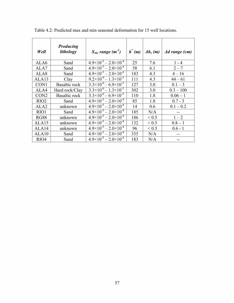
57

Table 4.2: Predicted max and min seasonal deformation for 15 well locations.

Well

Producing lithology

Sske range (m-1)

b* (m)

Δhs (m)

Δd range (cm)

ALA6 Sand 4.9×10-5 – 2.0×10-4 25 7.6 1 - 4 ALA7 Sand 4.9×10-5 – 2.0×10-4 58 6.1 2 – 7 ALA8 Sand 4.9×10-5 – 2.0×10-4 183 4.3 4 – 16 ALA13 Clay 9.2×10-4 – 1.3×10-3 111 4.3 44 – 61 CON1 Basaltic rock 3.3×10-6 – 6.9×10-5 127 3.0 0.1 – 3 ALA4 Hard rock/Clay 3.3×10-6 – 1.3×10-3 302 3.0 0.3 – 100 CON2 Basaltic rock 3.3×10-6 – 6.9×10-5 110 1.8 0.06 – 1 RIO2 Sand 4.9×10-5 – 2.0×10-4 85 1.8 0.7 - 3 ALA2 unknown 4.9×10-5 – 2.0×10-4 14 0.6 0.1 – 0.2 RIO1 Sand 4.9×10-5 – 2.0×10-4 185 N/A -- RG88 unknown 4.9×10-5 – 2.0×10-4 186 < 0.5 1 – 2

ALA15 unknown 4.9×10-5 – 2.0×10-4 132 < 0.5 0.8 – 1 ALA14 unknown 4.9×10-5 – 2.0×10-4 96 < 0.5 0.6 - 1 ALA10 Sand 4.9×10-5 – 2.0×10-4 335 N/A -- RIO4 Sand 4.9×10-5 – 2.0×10-4 183 N/A --

58

Chapter 5

Assessment of InSAR deformation data

5.1 Introduction

The goal of this thesis is to use InSAR deformation data to estimate hydraulic head

in the San Luis Valley (SLV), Colorado. The first step, and the focus of the present

chapter, is to determine whether high quality InSAR data can be obtained in the SLV.

The work completed in this chapter of the thesis was published in the journal Water

Resource Research [Reeves et al., 2011].

The SLV is an agricultural area, where crop growth, irrigation, land erosion, and

harvesting cycles can all seriously degrade the InSAR data by perturbing the positions of

individual radar scatterers. In contrast, the studies outlined below have been conducted

in: a) urban areas or b) arid to semi-arid climate regions. In both urban areas and arid

regions vegetation does not greatly interfere with the InSAR measurements.

59

A group of papers, beginning with the work done by Galloway et al. (1998), used InSAR

data to identify where deformation due to groundwater extraction was occurring

[Galloway et al., 1998; Amelung et al., 1999; Hoffmann et al., 2001; Bawden, 2002; Bell,

2002; Watson et al., 2002; Hoffmann et al., 2003; Schmidt and Burgmann, 2003; Canuti

et al., 2006; Chatterjee, 2006; Sneed et al., 2007; Anderssohn et al., 2008; Hung et al.,

2010; Wisely and Schmidt, 2010; Calderhead et al., 2011]. In many of these papers the

authors attempted to understand the hydrogeologic structure of the subsurface from the

InSAR deformation data. In most cases, in order to validate the data, the authors

compared the InSAR deformation measurements to those made with Global Positioning

Systems (GPS), leveling line surveys or extensometers.

However, in the SLV we do not have another surface deformation measurement to

validate the InSAR data. This was also the case for two other studies, in the Arno River

Basin, Italy by Canuti et al. (2006) and in the San Bernadino Basin, California by Wisely

and Schmidt (2010). In both of these studies the authors compared the InSAR

deformation measurements to seasonal trends in hydraulic head measurements for

validation. We will validate the InSAR deformation data collected from the SLV by:

evaluating the raw interferograms, quantifying the mean coherence of the deformation

data and comparing InSAR derived hydraulic head estimates to hydraulic head

measurements made in wells. We will use Small Baseline Subset (SBAS) analysis, as

described in section 2.1.2, to process the InSAR data. First, the individual interferograms

will be inspected for evidence of subsidence bowls due to seasonal grounwater pumping.

Then, the mean coherence (a proxy for the quality of the data) will be calculated for all of

60

the pixels in the SLV. The final line of sight (LOS) deformation time-series will be

compared to hydraulic head data at specific well locations. This comparison aims to

identify similar seasonal trends in the two datasets. Finally, the work presented here will

go a step farther than previous research, and attempt to predict hydraulic head from the

InSAR deformation data at specific well locations using compressibility parameters

derived from aquifer tests. In the short background section to follow we outline how

deformation measurements and aquifer tests measurements can be used to predict

hydraulic head.

5.2 Relating deformation to hydraulic head

The deformation of the ground surface, which is derived here from InSAR data, is

directly related to changes in the thickness of the confined aquifer due to recharge and

withdrawal of groundwater. We rearrange Equation 2.26 to show that the change in

aquifer thickness Δb is governed by the change in hydraulic head Δh and the elastic

skeletal storage coefficient Ske, a parameter that characterizes the skeletal compressibility

of the aquifer system [Riley, 1969]:

. (5.1)

This relationship is valid when the aquifer system is deforming elastically/recoverably. In

order for an aquifer system to be deforming elastically the effective stress must be less

than the preconsolidation stress, or equivalently the hydraulic head must be above the

minimum historical hydraulic head. We assume that Δb is equal to the deformation of the

61

ground surface as measured by InSAR, that Δh is the change in head measured in

monitoring wells, and that Ske is obtained from an aquifer test (as described in Section

3.2.2).

The storage coefficient, S, that is obtained from an aquifer test has two components:

, (5.2)

the elastic skeletal storage (Ske) and the component of storage due to the compaction of

water (Sw). In general Sw is small compared to Ske, so we are able to assume that Ske = S,

an assumption made throughout this study.

5.3 The Small Baseline Subset and interferograms

Given the challenges of working in an agricultural area discussed in section 2.1.3,

we implemented a version of Small Baseline Subset (SBAS) analysis that is specific to

groundwater applications. In some agricultural areas stable patches have been found

around farmed fields yielding InSAR data with high coherence [Meyer et al., 1996;

Massonnet and Feigl, 1998]. However, previous to this work no one has used SBAS

analysis to investigate a time-series of deformation from an agricultural area. In this

study the initial processing of the SAR data, up to and including phase unwrapping, was

computed using the Generic SAR (GSAR) software package developed by NORUT

[Larsen et al., 2005]. We used GSAR to create the spatial versus temporal baseline plot

by iteratively selecting the optimal thresholds. The thresholds were initially set low in

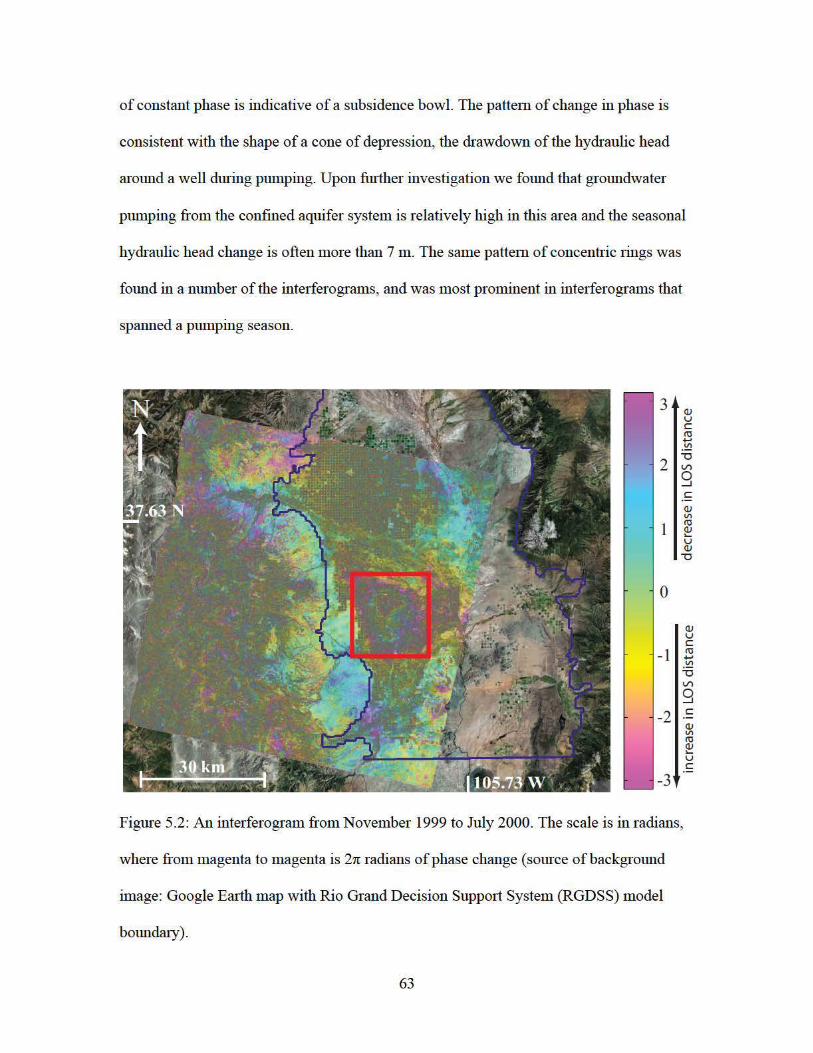
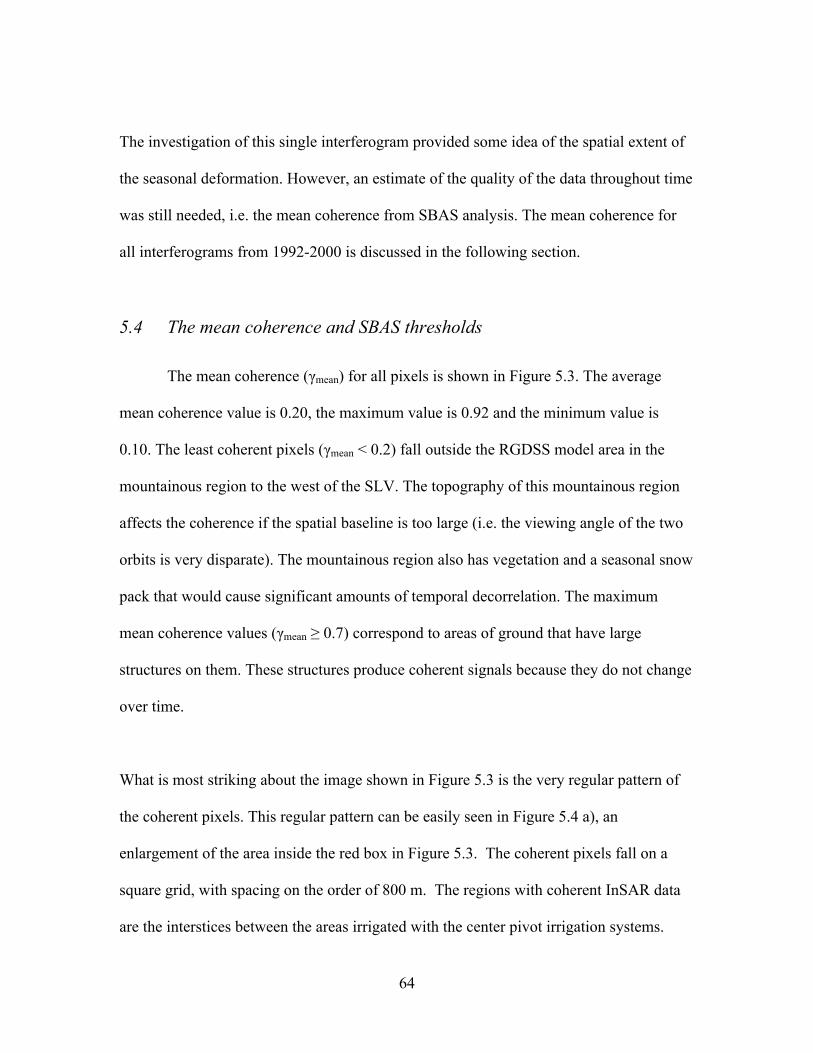
64

The investigation of this single interferogram provided some idea of the spatial extent of

the seasonal deformation. However, an estimate of the quality of the data throughout time

was still needed, i.e. the mean coherence from SBAS analysis. The mean coherence for

all interferograms from 1992-2000 is discussed in the following section.

5.4 The mean coherence and SBAS thresholds

The mean coherence (γmean) for all pixels is shown in Figure 5.3. The average

mean coherence value is 0.20, the maximum value is 0.92 and the minimum value is

0.10. The least coherent pixels (γmean < 0.2) fall outside the RGDSS model area in the

mountainous region to the west of the SLV. The topography of this mountainous region

affects the coherence if the spatial baseline is too large (i.e. the viewing angle of the two

orbits is very disparate). The mountainous region also has vegetation and a seasonal snow

pack that would cause significant amounts of temporal decorrelation. The maximum

mean coherence values (γmean ≥ 0.7) correspond to areas of ground that have large

structures on them. These structures produce coherent signals because they do not change

over time.

What is most striking about the image shown in Figure 5.3 is the very regular pattern of

the coherent pixels. This regular pattern can be easily seen in Figure 5.4 a), an

enlargement of the area inside the red box in Figure 5.3. The coherent pixels fall on a

square grid, with spacing on the order of 800 m. The regions with coherent InSAR data

are the interstices between the areas irrigated with the center pivot irrigation systems.

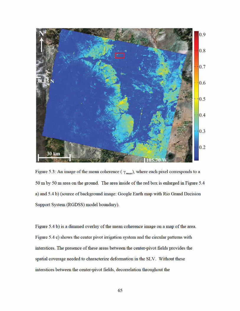
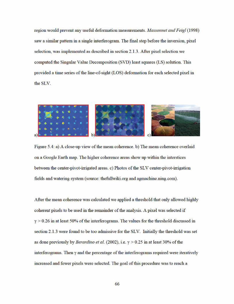
67

threshold that would require high coherence while still selecting pixels across the entire

SLV. The next section we describe how we modified conventional SBAS analysis for

groundwater applications in the SLV.

5.5 SBAS analysis modified for groundwater applications

Conventional SBAS analysis was discussed in section 2.1.3. As described in

Berardino et al. (2002) conventional SBAS analysis requires some prior information

about the deformation (low-pass deformation model), and that this deformation can be

expressed as a simple linear, quadratic or sinusoidal function. Some previous work

applying InSAR data to groundwater studies has used a sinusoidal function to capture the

seasonal deformation signal [Schmidt and Burgmann, 2003; Bell et al., 2008; Wisely and

Schmidt, 2010]. This prior information can be provided by GPS measurements, leveling

line surveys or extensometer measurements. These measurements are not available in the

SLV during the time of InSAR data acquisition, so a reliable low-pass model does not

exist. As is the case in many agricultural areas, the only data that exist in the SLV are

hydraulic head measurements made in wells screened in the confined aquifer system.

Figure 5.5 shows the hydraulic head as measured in well CON2 in the SLV. The seasonal

changes in head are due to variability groundwater pumping by agricultural water users

from one year to the next. Farmers in agricultural areas initially rely on surface water

resources to fulfill their irrigation needs. However, as precipitation levels vary from year

to year in some instances farmers need to extract more groundwater to sustain their crops.

If elastic deformation is assumed, the hydraulic head measurements in Figure 5.5 imply

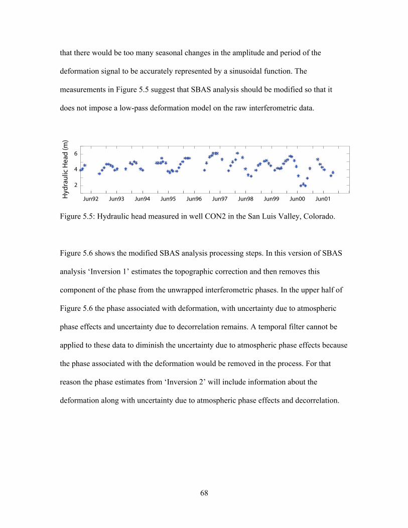
68

that there would be too many seasonal changes in the amplitude and period of the

deformation signal to be accurately represented by a sinusoidal function. The

measurements in Figure 5.5 suggest that SBAS analysis should be modified so that it

does not impose a low-pass deformation model on the raw interferometric data.

Figure 5.5: Hydraulic head measured in well CON2 in the San Luis Valley, Colorado.

Figure 5.6 shows the modified SBAS analysis processing steps. In this version of SBAS

analysis ‘Inversion 1’ estimates the topographic correction and then removes this

component of the phase from the unwrapped interferometric phases. In the upper half of

Figure 5.6 the phase associated with deformation, with uncertainty due to atmospheric

phase effects and uncertainty due to decorrelation remains. A temporal filter cannot be

applied to these data to diminish the uncertainty due to atmospheric phase effects because

the phase associated with the deformation would be removed in the process. For that

reason the phase estimates from ‘Inversion 2’ will include information about the

deformation along with uncertainty due to atmospheric phase effects and decorrelation.

Jun92 Jun93 Jun94 Jun95 Jun96 Jun97 Jun98 Jun99 Jun00 Jun01

2

4

6

Hyd

raul

ic H

ead

(m)

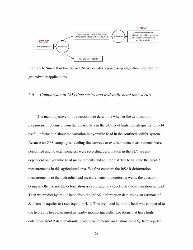
69

Figure 5.6: Small Baseline Subset (SBAS) analysis processing algorithm modified for

groundwater applications.

5.6 Comparison of LOS time series and hydraulic head time series

The main objective of this section is to determine whether the deformation

measurement obtained from the InSAR data in the SLV is of high enough quality to yield

useful information about the variation in hydraulic head in the confined aquifer system.

Because no GPS campaigns, leveling line surveys or extensometers measurements were

performed and no extensometers were recording deformation in the SLV we are

dependent on hydraulic head measurements and aquifer test data to validate the InSAR

measurements in this agricultural area. We first compare the InSAR deformation

measurements to the hydraulic head measurements in monitoring wells; the question

being whether or not the deformation is capturing the expected seasonal variation in head.

Then we predict hydraulic head from the InSAR deformation data, using an estimate of

Ske from an aquifer test (see equation 4.1). This predicted hydraulic head was compared to

the hydraulic head measured in nearby monitoring wells. Locations that have high

coherence InSAR data, hydraulic head measurements, and estimates of Ske from aquifer

Unwrapped phase

Topographic correction

Phase estimate at eachacquisition time, with uncertainty

due to atmospheric e!ectsand decorrelation

Inversion 1

Inversion 2Phase associated with deformation,

atmospheric e!ects and decorrelation

START

FINISH

70

tests, are needed to perform this analysis.

In the following paragraph we describe how we determined appropriate locations at

which to make the comparison between predicted and measured hydraulic head. As

discussed in section 4.2, there are only 11 wells where we predict that the deformation

will be large enough to be accurately measured by InSAR. There have been 151 aquifer

tests in the confined aquifer system, however, only 17 of them provide estimates of S.

There were six monitoring well/aquifer test well pairs that were collocated within 2 km of

each other. However, upon further inspection we found that three of the monitoring wells

either: a) did not exhibit seasonal pumping and recharge, or b) were not sampling the

same portion of the aquifer system as the aquifer test wells. Therefore, the final dataset

for comparison is: hydraulic head measurements from three monitoring wells and three

aquifer test wells with estimates of S. The highest coherence pixel within 1 km of the

monitoring well was selected to be the location of the LOS deformation measurements.

At each of the three monitoring well locations the background phase gradient was low

enough to justify a separation of 1 km. For these specific well locations this is a

reasonable assumption, however in Chapter 6 we will revisit this issue for all wells in the

SLV.

Figure 5.7, plots A), C) and E) show the LOS deformation time series for the three high

coherence pixels (red markers). The location of each of the deformation time series is

labeled as a cyan marker on Figure 5.8. The error in the InSAR measurement was

estimated to be ~ 6 mm (shown as error bars in Figure 5.7). In general little attention is

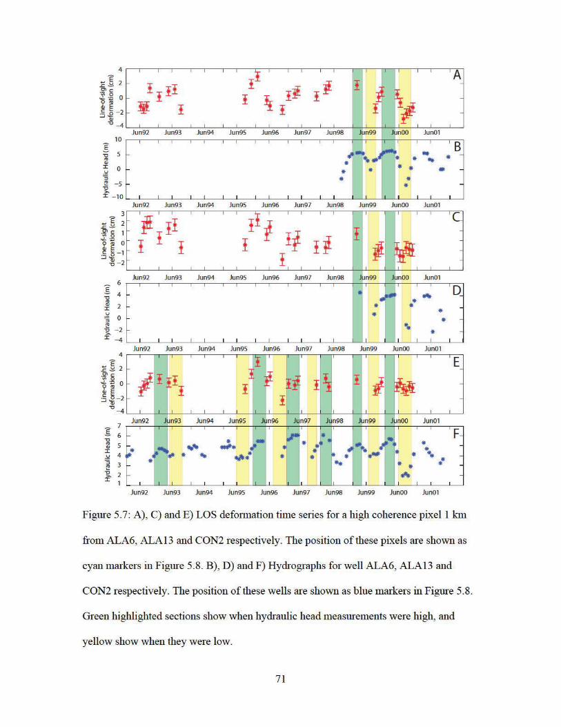
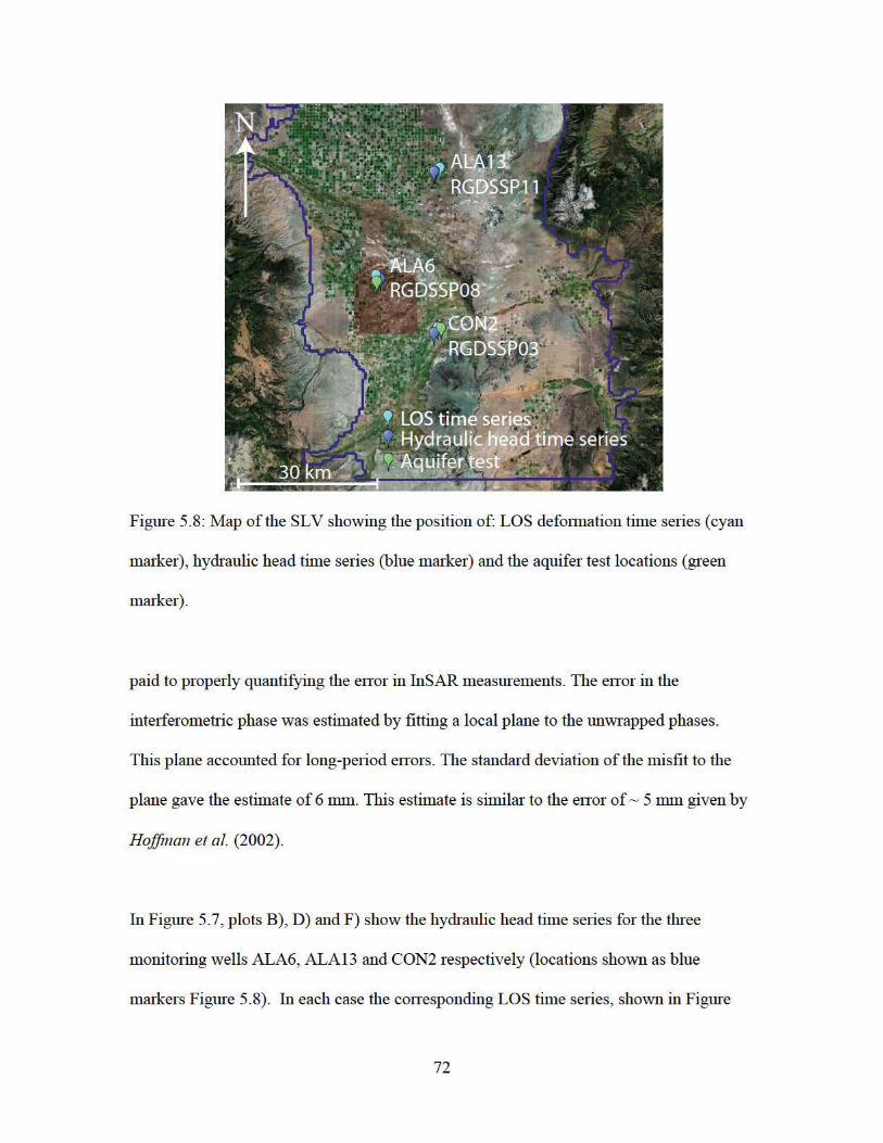
73

5.7 plots A), C), and E), are from the pixels with the highest coherence, within 1 km of

the monitoring wells. The deformation and hydraulic head should be linearly related via

the skeletal elastic storage coefficient Ske (Equation 5.1). Figure 5.7 shows that the two

time series appear to be linearly related.

We highlighted in green the times of the year when the hydraulic head in the monitoring

well is high, and in yellow the times when the hydraulic head is low, see Figure 5.7. We

compared hydraulic head and deformation only during time periods when both data were

acquired. For all but a few occasions we can see that when the hydraulic head is high, the

deformation indicates an upward movement of the ground surface, and when the

hydraulic head is low the deformation indicates a downward movement. In general, the

agreement of the two time-series is better at well ALA6 than at wells ALA13 and CON2.

This may be a result of both the hydraulic head change and the deformation exhibiting a

larger changes at this well location. Overall the periodicities of the measurements are in

good agreement, suggesting that the deformation we are measuring with InSAR in the

SLV is recording the seasonal changes in the hydraulic head in the confined aquifer

system. This in itself is very useful information that could be used in a qualitative way to

indicate when and where significant changes in head occur. In addition, as can be seen in

Figure 5.7, InSAR provides us with data at times before head measurements were being

made in many of the wells in the SLV. This longer period of monitoring is valuable for

assessing long-term changes in the aquifer. For example, one important observation that

can be made is the absence of a significant negative linear trend in the deformation in

74

Figure 5.7 A), C), and E). This supports the assumption that only elastic deformation is

occurring in these regions of the SLV.

For each of the 11 wells described in section 4.2 (ALA6, ALA13 and CON2 inclusive)

we estimated the linear trend in the deformation time-series. We found that all of the

linear trends were negative, with a mean of approximately -0.07 cm/year. The linear trend

at well RG88 was the largest (-0.15 cm/year). However, both the mean and the maximum

value are both small enough to conclude that the deformation occurring at these well

locations is elastic. This is a particularly important result, as it is at these well locations

that we expected the deformation to be the largest, according to our initial calculations in

Chapter 4.

5.7 Head estimates from InSAR deformation and aquifer test data

As a final validation of the deformation data, we estimated hydraulic head, derived

from InSAR deformation data, and compared it to the measured Δh at the three

monitoring wells (ALA6, ALA13, CON2). However, in order to make this comparison

Δb (InSAR data) and Ske (aquifer test well data) are required at the monitoring well

locations (see Equation 5.1). As previously stated in section 5.6, we assumed that the

deformation measured at the high coherence pixel is approximately the same as the

deformation at the monitoring well (~1 km away). The aquifer test wells are: RGDSSP08,

RGDSSP11 and RGDSSP03 (locations shown as green markers in Figure 5.8). The

distance between aquifer test wells and monitoring wells is as follows: RGDSSP08 is 300

m from ALA6, RGDSSP11 is 100 m from ALA13 and RGDSSP03 is 2 km from CON2.

75

In order to use the estimates of

�

S from the aquifer tests at the monitoring well locations

the thickness of the producing zone, i.e. the thickness of the aquifer from which water is

being withdrawn, for each well needs to be known.

During an aquifer test the obtained value of

�

S depends upon the producing zone

thicknesses (

�

b*) at the aquifer test well:

, (5.2)

where Ss is the specific storage. The monitoring well and aquifer test well pairs were all

producing from similar hydrogeologic units, and hence should exhibit similar values of

Ss. However, the thickness of the producing zone varied because the wells were screened

over different intervals. In order to use the value of

�

S from the aquifer test well at the

monitoring well location this disparity needed to be corrected for. The screened interval

was used as the producing zone thickness at the aquifer test wells based on the

assumption that flow into the well is horizontal: 23.8 m at RGDSSP08, 75.3 m at

RGDSSP11 and 150.9 m at RGDSSP03. This producing zone thickness was used to

calculate the specific storage, Ss = S / b*. Using Ss and the producing zone thickness at the

monitoring wells: 25.3 m at ALA6, 111.3 m at ALA13 and 110.0 m at CON2,

�

S was

calculated at the monitoring wells: S =1.4 × 10-3 for ALA6, S =7.8 × 10-4 for ALA13 and

S =1.7 × 10-3 for CON2. As discussed in section 5.2 the storage from the expansion and

contraction of water (Sw) was assumed to be small, such that S can act as a proxy for Ske.

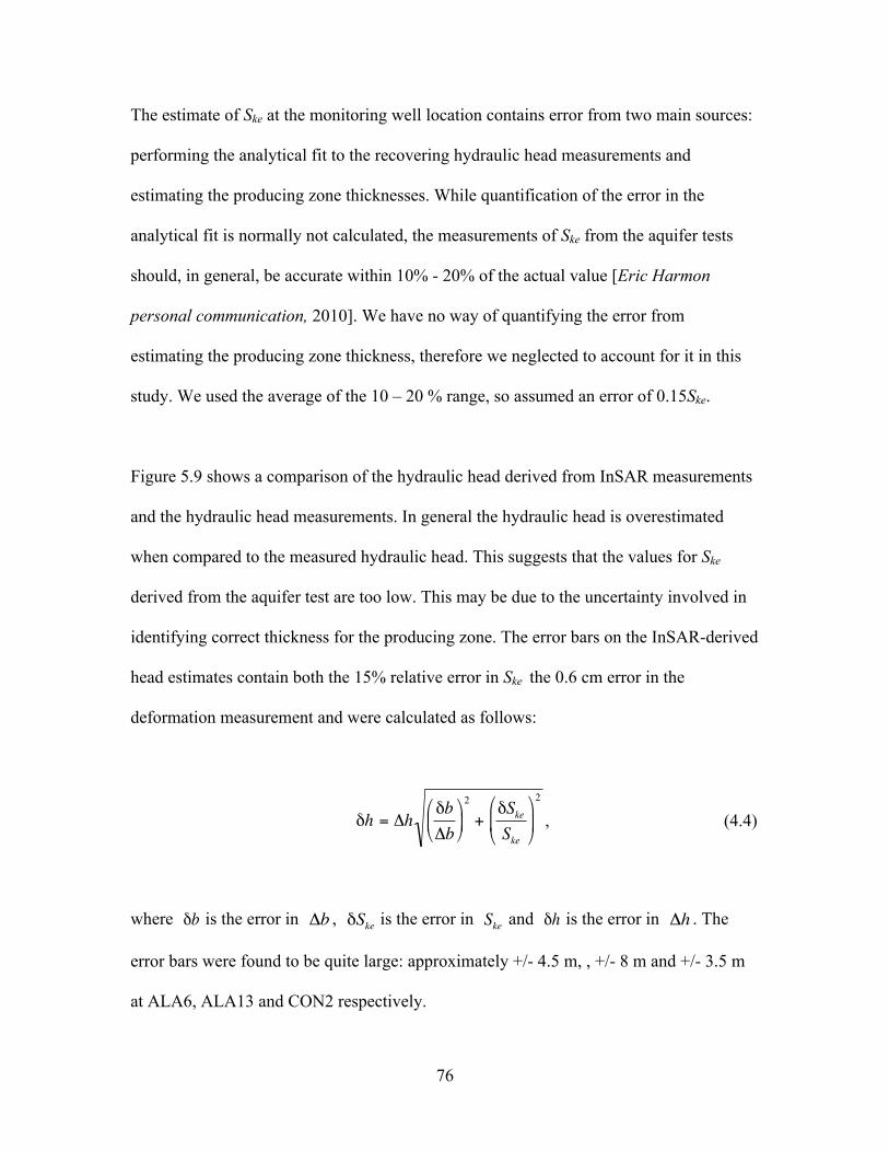
76

The estimate of Ske at the monitoring well location contains error from two main sources:

performing the analytical fit to the recovering hydraulic head measurements and

estimating the producing zone thicknesses. While quantification of the error in the

analytical fit is normally not calculated, the measurements of Ske from the aquifer tests

should, in general, be accurate within 10% - 20% of the actual value [Eric Harmon

personal communication, 2010]. We have no way of quantifying the error from

estimating the producing zone thickness, therefore we neglected to account for it in this

study. We used the average of the 10 – 20 % range, so assumed an error of 0.15Ske.

Figure 5.9 shows a comparison of the hydraulic head derived from InSAR measurements

and the hydraulic head measurements. In general the hydraulic head is overestimated

when compared to the measured hydraulic head. This suggests that the values for Ske

derived from the aquifer test are too low. This may be due to the uncertainty involved in

identifying correct thickness for the producing zone. The error bars on the InSAR-derived

head estimates contain both the 15% relative error in Ske the 0.6 cm error in the

deformation measurement and were calculated as follows:

, (4.4)

where is the error in , is the error in and is the error in . The

error bars were found to be quite large: approximately +/- 4.5 m, , +/- 8 m and +/- 3.5 m

at ALA6, ALA13 and CON2 respectively.

€

δh = ΔhδbΔb$

% &

'

( ) 2

+δSkeSke

$

% &

'

( )

2

€

δb

€

Δb

€

δSke

€

Ske

€

δh

€

Δh

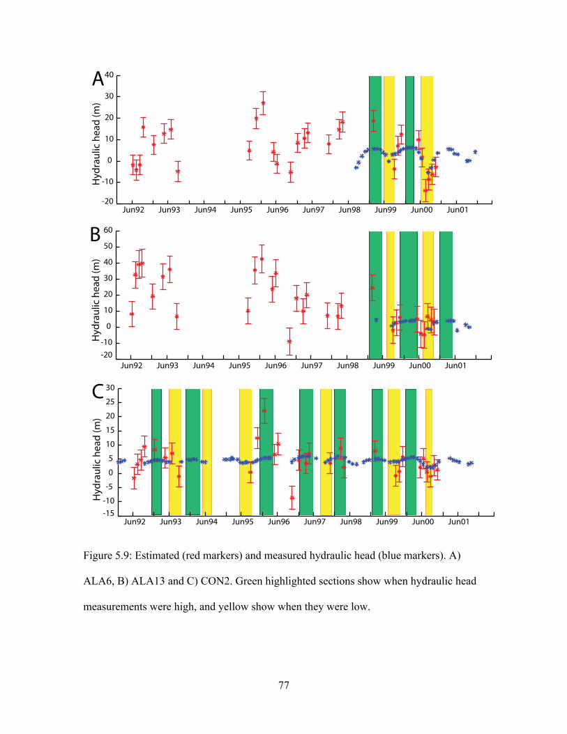
77

Figure 5.9: Estimated (red markers) and measured hydraulic head (blue markers). A)

ALA6, B) ALA13 and C) CON2. Green highlighted sections show when hydraulic head

measurements were high, and yellow show when they were low.

Hyd

raul

ic h

ead

(m)

Hyd

raul

ic h

ead

(m)

A

C

B

-20-10

0

10

20

30

40

50

60

-15-10

-5

0

5

10

15

20

25

30

Hyd

raul

ic h

ead

(m)

Jun92 Jun93 Jun94 Jun95 Jun96 Jun97 Jun98 Jun99 Jun00 Jun01-20

-10

0

10

20

30

40



78

In many instances, as shown in Figure 5.9, the measured hydraulic head falls within the

error bars of the estimated hydraulic head values. At well ALA6, five of the ten InSAR-

derived head estimates fall within the error bars of the measured values; at ALA13, 9 of

10 agree; and at well CON 2, 20 of 31 agree. However, as discussed earlier, the error bars

calculated were very large compared to the hydraulic head changes measured in the

monitoring wells. Future research should focus on improving our ability to accurately

determine the uncertainty in both from aquifer tests as well as from the InSAR

measurements. Only then will the method described above become a viable tool for

predicting hydraulic head.

A number of spurious points occur in the InSAR-derived hydraulic head estimates: in

February 1996 a large amount of upward deformation occurred and in November 1996 a

large amount of downward deformation occurred. These outliers could have been caused

by atmospheric phase effects. As described in section 5.5 the LOS deformation time-

series was not filtered temporally to remove atmospheric phase effects.

5.8 Conclusions

Our first finding of significance in this thesis was the discovery that many of the

small areas, left unwatered by the center-pivot irrigation systems, yielded high quality

InSAR data when processed using SBAS methods. The InSAR deformation

measurements showed the same seasonal periodicity as the hydraulic head data from

monitoring wells. We also found that only elastic deformation was occurring from 1992 –

2000 at the 11 well locations identified in Chapter 4. This is a significant result in itself,

79

as it speaks towards the sustainability of groundwater extraction from the confined

aquifer system.

When hydraulic head was estimated from the InSAR data, we found good agreement

between the estimated hydraulic head and the measured head values (within the error

bars). However, we acknowledge that the errors are so large that these hydraulic head

estimates would not provide the level of accuracy required for the RGDSS. The

uncertainty in the hydraulic head estimates is dependent on the uncertainty in Ske and the

uncertainty in the InSAR deformation measurements. It is clear that more research is

required to understand how best to predict head from InSAR data. Can this be done using

the field measurements of Ske if we can improve the accuracy of the measurement? Or

should we assume that the use of InSAR data to obtain head estimates will always require

calibration, with wells in selected regions instrumented specifically for this purpose? In

either case an improved understanding of the uncertainty in the InSAR deformation

measurement is necessary before these data can be used for groundwater applications.

Therefore, Chapter 6 will focus on quantifying the spatially variable uncertainty in the

InSAR deformation measurement. In Chapter 7 of this thesis we will revisit the issue of

calibration by investigating the relationship between deformation and hydraulic head at

the 11 confined aquifer wells from Chapter 4.

Despite the fact that we cannot yet accurately obtain hydraulic head estimates from the

InSAR data, we conclude that we can obtain high quality InSAR data from the SLV, and

that these data capture useful information about the seasonal variability in head. Once we

80

determine how to accurately obtain hydraulic head from InSAR data, it is easy to see

from Figure 5.9 that a host of new data will become available to water managers. For

example, at ALA6 and ALA13, where hydraulic head data have only been collected since

1999 the InSAR data will be able to provide estimates of hydraulic head back to 1992.

The hope is that InSAR data from this region can also be used going forward as an

integral part of hydrogeologic modeling and monitoring in the valley.

81

Chapter 6

Quantifying uncertainty in the InSAR measurement

6.1 Introduction

In the previous chapter we showed that Interferometric Synthetic Aperture Radar

(InSAR) deformation measurements exhibit seasonal trends similar to hydraulic head

levels in the confined aquifer system of an agricultural area. However, when we

attempted to obtain hydraulic head from the InSAR deformation measurements we found

that our estimate of the uncertainty of these measurements was not sufficiently accurate.

Moreover, for our initial analysis of InSAR data quality in Chapter 5 we used the closest

high quality pixel to the well location to make the comparison with hydraulic head.

Figure 6.1a) shows high quality InSAR data from an urban/arid area and Figure 6.1b)

shows the sparse high quality data from vegetated areas like the San Luis Valley (SLV).

Because we know that the quality of the data, i.e. the coherence, is changing from pixel to

pixel in vegetated areas of the SLV it would be ideal to determine the exact uncertainty at

each pixel before we revisit the relationship between deformation and hydraulic head

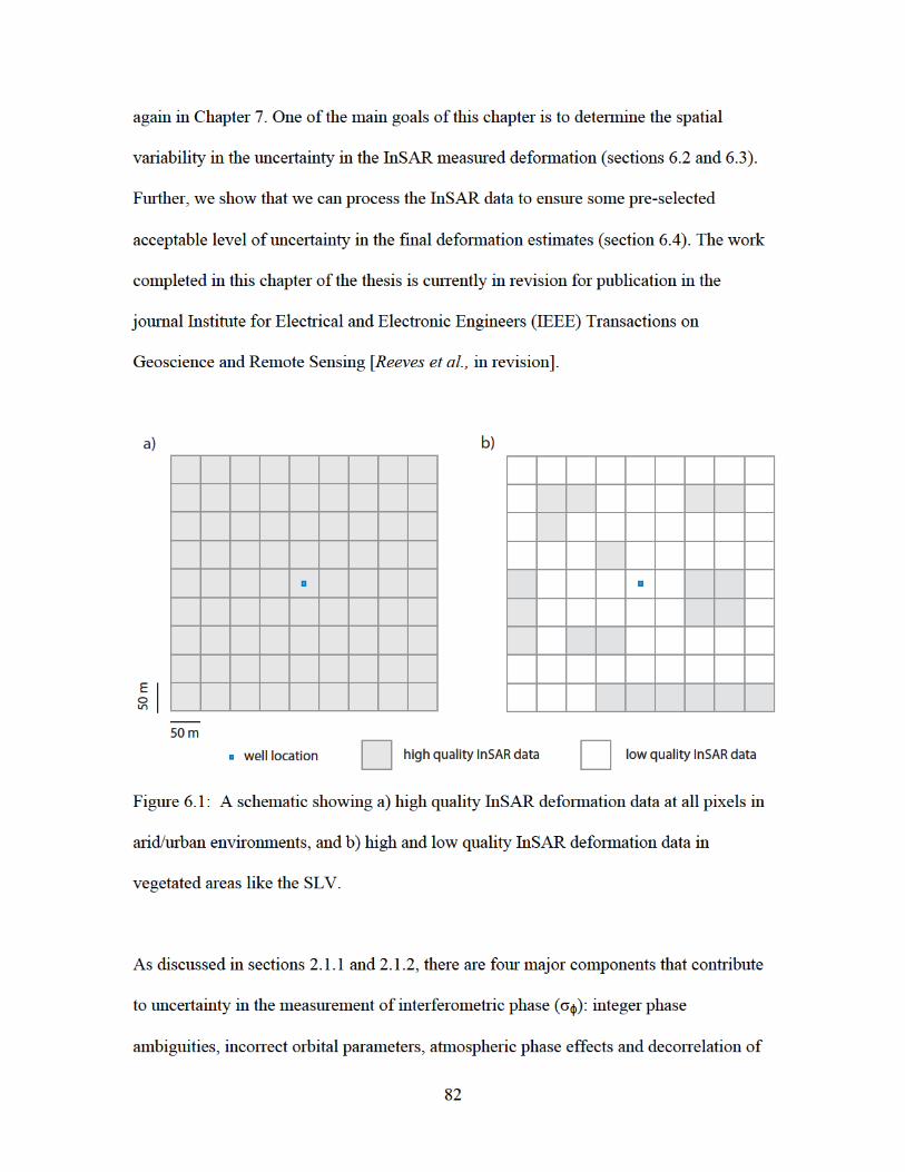
83

radar signals. These components were discussed at length in Hanssen (2001). In this

chapter we address two of these components: atmospheric phase effects and decorrelation

of radar signals, as we have found that these two components have the largest effect on

the uncertainty of the InSAR deformation measurement in the SLV. The other two

components, integer phase ambiguities and incorrect orbital parameters, do not have a

large effect on the uncertainty in the SLV and were previously discussed in section 2.1.1

and 2.1.2.

As discussed in section 2.1.2 a number of studies have attempted to quantify the

uncertainty due to atmospheric phase effects (Onn and Zebker, 2006; Knospe and

Jonsson, 2010). Instead of directly modeling the uncertainty due to this component, as

done in the two studies mentioned above, we propose using supplementary hydrologic

data from the SLV in order to identify which scenes may contain large amounts of

atmospheric phase effects and then eliminating them from our analysis. In section 6.2 of

this chapter we demonstrate our proposed methodology, first on a synthetic data set and

then on data from the SLV.

Once we reduce the uncertainty due to atmospheric phase effects by eliminating the

noisiest scenes, the dominant remaining component of uncertainty is associated with the

decorrelation of radar signals. Two seminal studies, Zebker and Villasenor (1992) and

Hanssen (2001) have quantified the uncertainty in the interferometric phase due to

decorrelation. However, in studies where the data are being used to better understand a

physical process (e.g., an earthquake, a volcanic eruption, or groundwater extraction)

84

most authors avoid propagating this component of uncertainty through the InSAR

processing chain. Propagating these uncertainties is computationally intensive and often

Global Positioning System (GPS) measurements are instead used to validate the data.

Also, in general, most studies have looked at large magnitude deformation that was well

understood and easily modeled. In the SLV we are measuring smaller seasonal signals

that take place over short timescales. In our case the uncertainty due to decorrelation may

have a large impact on our results. A few studies applying multi-temporal techniques

(small baseline subset (SBAS) analysis or persistent scatterer (PS) analysis) have

considered propagating uncertainty due to decorrelation through the processing chain

[Hooper et al., 2004; Kwoun et al., 2006; Guarnieri and Tebaldini, 2007; Rocca, 2007;

Anderssohn et al., 2009; Gonzalez and Fernandez, 2011].

In this chapter we use SBAS analysis to process our InSAR data. In non-urban terrains,

like the SLV, the scattering mechanism for the EM waves is described as distributed. For

distributed scattering all scattering elements in a resolution cell reflect the EM wave with

the same strength. SBAS analysis is an appropriate technique for processing data in areas

where a distributed scattering mechanism dominates [Agram, 2010]. In section 6.3 we

take a similar approach and propagate the uncertainty due to decorrelation through the

SBAS analysis processing chain for all 1.5 million pixels in the SLV. In order to do so we

use the modified SBAS analysis presented in section 5.5 to accommodate signal

characteristics specific to groundwater applications and we describe mathematically how

uncertainty propagates through this processing chain. This methodology provides a

measure of uncertainty for each deformation estimate at each acquisition time.

85

There are two decision points during SBAS analysis processing where we answer the

following questions: a) what should the spatial and temporal baseline thresholds be, and

b) what is an acceptable threshold for the decorrelation of a pixel? Setting the thresholds

for the spatial and temporal baselines limits the number of interferograms used in SBAS

analysis, and setting the threshold for the decorrelation limits the number of pixels

selected for further processing. These thresholds have previously been set in a fairly ad

hoc manner [Berardino et al., 2002; Lauknes, 2004]. In section 6.4 we determine

appropriate threshold parameters in order to meet some predetermined level of

uncertainty in the final deformation time-series.

The ultimate goal of our research is to find a way to use InSAR deformation

measurements to obtain hydraulic head in confined aquifer systems. Quantifying the

spatial variability of the uncertainty in the deformation measurement is an important step

in this process. We begin our study by outlining an algorithm that uses additional

hydrologic data to diminish the amount of uncertainty due to atmospheric phase effects.

6.2 Atmospheric Uncertainty in the SLV

Quantifying the uncertainty in the InSAR deformation estimate due to

atmospheric phase effects can be very complicated. The structure of the atmosphere used

to model these effects is often oversimplified and model results do not accurately

represent the atmospheric phase signal seen in real data. Because this component of the

uncertainty is difficult to quantify, we have decided to use supplementary hydrologic data

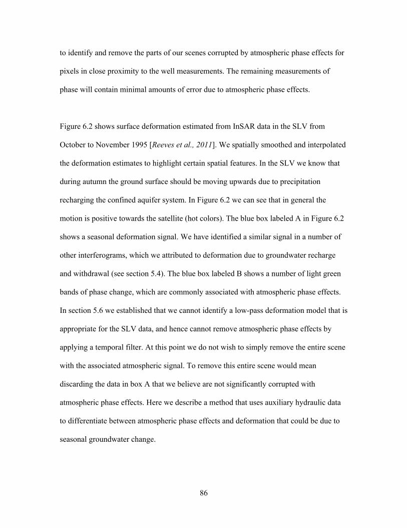
86

to identify and remove the parts of our scenes corrupted by atmospheric phase effects for

pixels in close proximity to the well measurements. The remaining measurements of

phase will contain minimal amounts of error due to atmospheric phase effects.

Figure 6.2 shows surface deformation estimated from InSAR data in the SLV from

October to November 1995 [Reeves et al., 2011]. We spatially smoothed and interpolated

the deformation estimates to highlight certain spatial features. In the SLV we know that

during autumn the ground surface should be moving upwards due to precipitation

recharging the confined aquifer system. In Figure 6.2 we can see that in general the

motion is positive towards the satellite (hot colors). The blue box labeled A in Figure 6.2

shows a seasonal deformation signal. We have identified a similar signal in a number of

other interferograms, which we attributed to deformation due to groundwater recharge

and withdrawal (see section 5.4). The blue box labeled B shows a number of light green

bands of phase change, which are commonly associated with atmospheric phase effects.

In section 5.6 we established that we cannot identify a low-pass deformation model that is

appropriate for the SLV data, and hence cannot remove atmospheric phase effects by

applying a temporal filter. At this point we do not wish to simply remove the entire scene

with the associated atmospheric signal. To remove this entire scene would mean

discarding the data in box A that we believe are not significantly corrupted with

atmospheric phase effects. Here we describe a method that uses auxiliary hydraulic data

to differentiate between atmospheric phase effects and deformation that could be due to

seasonal groundwater change.

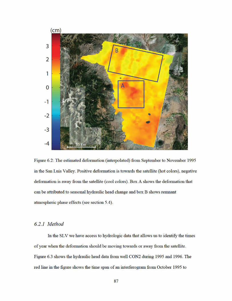
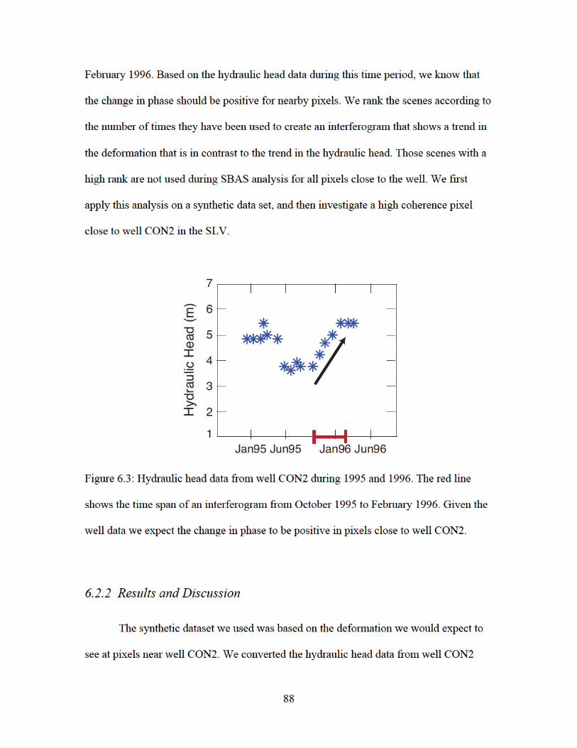
89

into deformation by assuming elastic deformation (equation 5.1). We assumed that Δb is

equal to the deformation of the ground surface as measured by InSAR and that Ske ≈

0.003, a reasonable value for this area of the SLV [RGDSS, 2005]. We added Gaussian

white noise such that the signal to noise ratio (SNR) of the synthetic dataset was ~ 20 dB.

We converted the deformation measurements into phase measurements based on ERS-1

and ERS-2 system parameters. In Figure 6.4 the solid blue line shows the synthetic data,

phase as a function of time.

To generate the synthetic data,we randomly selected 30 acquisition times, and added a

phase delay simulating atmospheric phase effects to three random scenes (December

1999, December 2000, and September 2001). We assigned random spatial baselines to

the scenes and created interferograms for scene pairs with a perpendicular baseline of less

than 400 m and a temporal baseline of less than 4 years. We then applied the algorithm as

described in section 6.2.1, the result of which is a list of ranked scenes. We removed the

scene with the highest rank, and repeated the algorithm iteratively. The algorithm was

finished when the scenes remaining were those which had been used in only one

interferogram showing deformation opposite to the trend predicted from the head

measurements.

We then removed the scenes that the algorithm identified as containing significant

atmospheric phase effects and solved for the phase at each acquisition time. Figure 6.4

shows the phase estimates in red, when we used all the scenes, including the ones

containing atmospheric phase effects, and phase estimates in blue when we removed

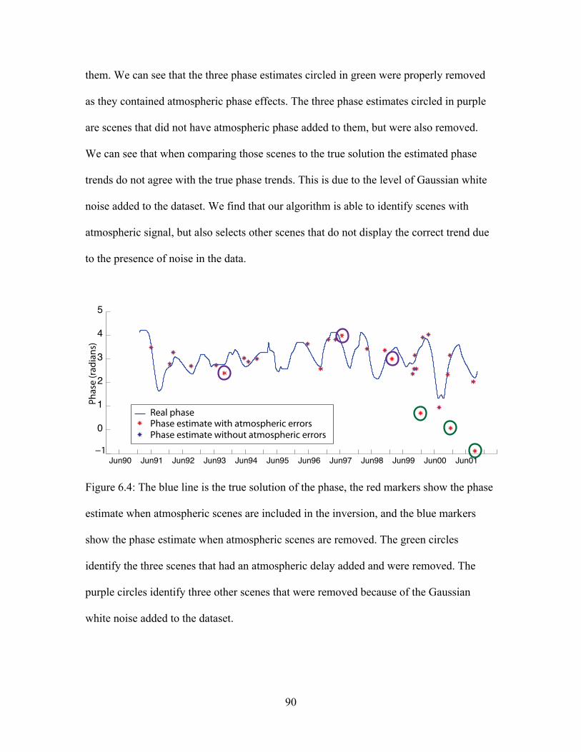
90

them. We can see that the three phase estimates circled in green were properly removed

as they contained atmospheric phase effects. The three phase estimates circled in purple

are scenes that did not have atmospheric phase added to them, but were also removed.

We can see that when comparing those scenes to the true solution the estimated phase

trends do not agree with the true phase trends. This is due to the level of Gaussian white

noise added to the dataset. We find that our algorithm is able to identify scenes with

atmospheric signal, but also selects other scenes that do not display the correct trend due

to the presence of noise in the data.

Figure 6.4: The blue line is the true solution of the phase, the red markers show the phase

estimate when atmospheric scenes are included in the inversion, and the blue markers

show the phase estimate when atmospheric scenes are removed. The green circles

identify the three scenes that had an atmospheric delay added and were removed. The

purple circles identify three other scenes that were removed because of the Gaussian

white noise added to the dataset.

Jun90 Jun91 Jun92 Jun93 Jun94 Jun95 Jun96 Jun97 Jun98 Jun99 Jun00 Jun01!1

0

1

2

3

4

5

Phas

e (ra

dian

s)

Real phasePhase estimate with atmospheric errorsPhase estimate without atmospheric errors

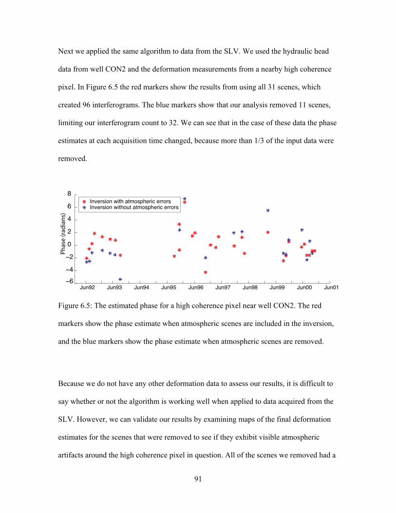
91

Next we applied the same algorithm to data from the SLV. We used the hydraulic head

data from well CON2 and the deformation measurements from a nearby high coherence

pixel. In Figure 6.5 the red markers show the results from using all 31 scenes, which

created 96 interferograms. The blue markers show that our analysis removed 11 scenes,

limiting our interferogram count to 32. We can see that in the case of these data the phase

estimates at each acquisition time changed, because more than 1/3 of the input data were

removed.

Figure 6.5: The estimated phase for a high coherence pixel near well CON2. The red

markers show the phase estimate when atmospheric scenes are included in the inversion,

and the blue markers show the phase estimate when atmospheric scenes are removed.

Because we do not have any other deformation data to assess our results, it is difficult to

say whether or not the algorithm is working well when applied to data acquired from the

SLV. However, we can validate our results by examining maps of the final deformation

estimates for the scenes that were removed to see if they exhibit visible atmospheric

artifacts around the high coherence pixel in question. All of the scenes we removed had a

Jun92 Jun93 Jun94 Jun95 Jun96 Jun97 Jun98 Jun99 Jun00 Jun01!6!4!202468

Phas

e (ra

dian

s)

Inversion with atmospheric errorsInversion without atmospheric errors

92

pattern structure that resembled atmospheric phase effects near well CON2. However, it

is also important to note that patterns that show atmospheric phase effects can take many

different forms [Knospe and Johnsson, 2010]. Both scenes that were used to create the

deformation in Figure 6.2 were removed, September 1995 and November 1995. This

technique shows an inherent trade off between the amount of atmospheric signal that

remains in the final time series and adequate sampling of the final time series. Although

we are not able to quantify the uncertainty due to atmospheric phase effects we are at

least able to remove the scenes, on a pixel-by-pixel basis, that may contain large amounts

of uncertainty in measured deformation due to atmospheric phase effects.

6.3 Propagation of uncertainty due to decorrelation

Now that we have proposed a method to reduce the uncertainty due to

atmospheric phase effects we can continue our investigation by propagating the

uncertainty in the interferometric phase through the SBAS analysis processing chain. In

section 6.1 we stated that we could only quantify the uncertainty due to decorrelation,

which is quantified by the coherence. The sections to follow will focus solely on this

component of the uncertainty.

6.3.1 Uncertainty in the interferometric phase

We define the uncertainty in the interferometric phase measurement as its

standard deviation (σ):

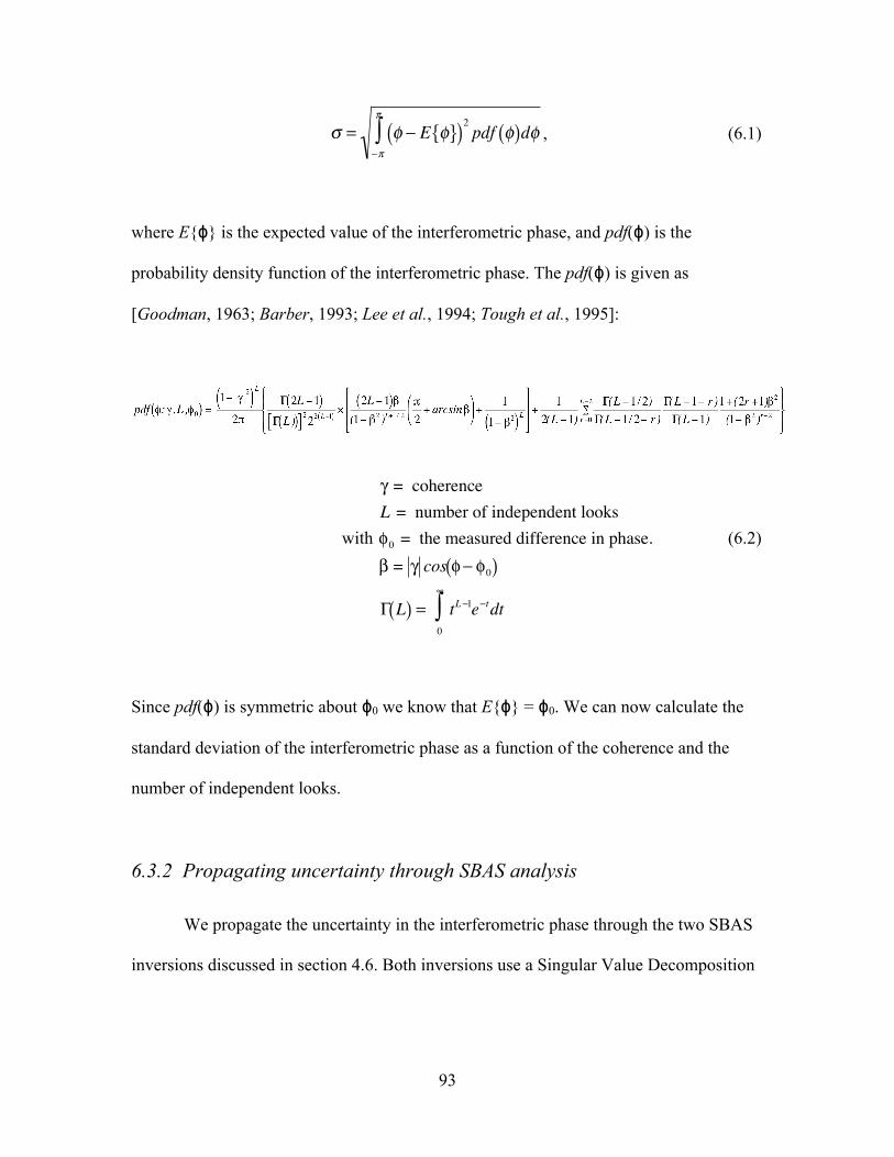
93

�

σ = φ − E φ{ }( )2 pdf φ( )dφ−π

π

∫ , (6.1)

where E{ϕ} is the expected value of the interferometric phase, and pdf(ϕ) is the

probability density function of the interferometric phase. The pdf(ϕ) is given as

[Goodman, 1963; Barber, 1993; Lee et al., 1994; Tough et al., 1995]:

with

�

γ = coherenceL = number of independent looksφ0 = the measured difference in phaseβ = γ cos φ− φ0( )

Γ L( ) = tL−1e−tdt0

∞

∫

. (6.2)

Since pdf(ϕ) is symmetric about ϕ0 we know that E{ϕ} = ϕ0. We can now calculate the

standard deviation of the interferometric phase as a function of the coherence and the

number of independent looks.

6.3.2 Propagating uncertainty through SBAS analysis

We propagate the uncertainty in the interferometric phase through the two SBAS

inversions discussed in section 4.6. Both inversions use a Singular Value Decomposition

94

(SVD) to calculate the generalized inverse (Ggen) of the design matrix (G). Using Ggen

and the data covariance matrix (Σd) we can calculate the model covariance as follows:

�

Σm = GgenΣd Ggen( )T . (6.3)

Below we will outline how to create the

�

Σd for both ‘Inversion 1’ and ‘Inversion 2’ from

Figure 5.6.

In ‘Inversion 1’ we estimate the topographic correction (Δz). We will need the data

covariance matrix (Σd) for the interferometric phases in order to propagate the uncertainty

through this inversion. Along the diagonal of Σd are interferometric phase variances, σ2.

However, interferograms that are made using a common scene have an associated data

covariance; these appear as off diagonal values in Σd. In the calculations to follow we will

show how we arrived at the data covariance for two interferograms that are formed with a

common scene.

The measured phase for a single scene is denoted by

�

ψ. This phase has a deterministic

component (d) and a stochastic component (r), such that ψ = d + r. The interferometric

phase (ϕ) for an interferogram formed between two scenes at time 1 and time 2 is as

follows:

. (6.4)

€

φ12 =ψ1 −ψ2

95

If we also have an interferogram formed between a scene at time 2 and a scene at time 3,

then the interferometric phase would be given by:

. (6.5)

Because the measurement ψ2 is a component of both ϕ12 and ϕ23 we suggest that the two

interferometric phases are correlated. More formally, we need to find the covariance of

two interferometric phase measurements, in this example ϕ12 and ϕ23:

. (6.6)

We can then substitute ψ1 = d1 + r1, ψ2 = d2 + r2, and ψ3 = d3 + r3 into the first four terms

of the above equation:

. (6.7)

If we expand the first four terms we can remove the terms involving E(dmrn) or E(rmrn)

because they are not correlated and their expected value will be zero. This leaves the

following:

€

φ23 =ψ2 −ψ3

€

Cov(φ12,φ23 ) = E(φ12φ23 ) − E(φ12 )E(φ23 ) = E((ψ1 −ψ2 )(ψ2 −ψ3 ))− (d1 − d2 )(d2 − d3 ) = E(ψ1ψ2 ) − E(ψ1ψ3 ) − E(ψ2ψ2 ) + E(ψ2ψ3 ) − d1d2 + d1d3 + d2d2 − d2d3

€

Cov(φ12,φ23 ) = E((d1 + r1)(d2 + r2 )) − E((d1 + r1)(d3 + r3 )) − E((d2 + r2 )(d2 + r2 ))+ E((d2 + r2 )(d3 + r3 ))... ...− d1d2 + d1d3 + d2d2 − d2d3

96

. (6.8)

If we know the variance of ϕ12 then we can show that:

. (6.9)

If we assume that Var(r1) = Var(r2), then Var(ϕ12) = 2E(r22), and we can calculate the

covariance given above. A similar calculation yields Var(ϕ23) = 2E(r22). However,

because we know that the coherence changes for each interferogram we infer that

Var(ϕ12) is not equal to Var(ϕ23). In order to reconcile this difference we use the average

of Var(ϕ12) and Var(ϕ23) for the expectation. In doing so, we achieve physically plausible

results, although we know that there are other unidentified systematic errors that are

neglected in our analysis. We find that this is the best way to honor the data covariance

between interferograms without knowing the joint probability density functions for the

measured phases. Therefore the final estimate of the covariance is as follows:

�

Cov(φ12,φ23 ) = −E(r22 ) = −

Var(φ12 ) +Var(φ23 )2

⎛ ⎝ ⎜

⎞ ⎠ ⎟ .

(6.10)

€

Cov(φ12,φ23 ) = E(d1d2 ) − E(d1d3 ) − E(d2d2 ) − E(r2r2 ) + E(d2d3 ) − d1d2 + d1d3 + d2d2 − d2d3 = −E(r2

2 )

97

Σd has the interferometric phase variances along the diagonal and covariances for

interferograms derived from a common scene for all non-zero off diagonal elements.

Using equation 6.3 we calculate Σm, which gives us the variance of the topographic

correction Var(Δz).

Once we estimate Δz from ‘Inversion 1’ we need to remove this component of the phase

from the measured interferometric phase:

�

ΔφD = Δφ − cΔz (6.11)

where Δϕd are the components of the phase measurement due to deformation and Δϕ are

the measured interferometric phases. The matrix c describes how Δz, estimated in

meters, can be converted into phase

�

c =4πBperp

λr sinθ, (6.12)

where λ is the wavelength, Bperp is the perpendicular component of the baseline between

satellite locations at acquisition, r is the range distance and θ is the incidence angle with

respect to Earth’s surface [Berardino et al., 2002]. Although recent research suggests that

using the difference between Bperp(scene1,reference) and Bperp(scene2,reference) is more

accurate, during initial synthetic studies we found that using Bperp for the interferogram

was sufficient for our analysis [Fattahi and Amelung, 2013]. Δϕd are the data for

‘Inversion 2’ in Figure 5.6. We now need to construct the data covariance matrix for Δϕd.

98

We can calculate the variance of the phase measurement due to deformation for

interferogram 1 (ΔϕD1 ) as follows:

. (6.13)

We know that

�

Δˆ z = c−1Δφ from ‘Inversion 1’, where c-1 is the generalized inverse of c

and Δϕ is the vector containing the interferometric phases. If we substitute that into the

second term in equation 6.11 and simplify we get:

. (6.14)

The covariance is calculated in a similar way. We can use the example of

ΔϕD1 = Δϕ1 – c(1,1) Δz and ΔϕD2 = Δϕ2 – c(2,1) Δz :

.(6.15)

Σd has the variances of ΔϕD along the diagonal and the covariances of ΔϕD for

interferograms that were made using a common scene for all non-zero off diagonal

elements. Once again, using equation 6.3 we can calculate Σm, which gives us the

€

Var(ΔφD1) = E(ΔφD12) − E(ΔφD1)

2

= E((Δφ1 − c(1,1)Δz)2) − E(Δφ1 − c(1,1)Δz)2

= E(Δφ12) − 2c(1,1)E(Δφ1Δz) + c(1,1)2E(Δz2) − (E(Δφ1) − c(1,1)E(Δz))2

€

Var(ΔφD1) = E(Δφ12) − 2c(1,1) ⋅ c −1E(Δφ1Δφ ) + c(1,1)2E(Δz2) − (E(Δφ1) − c(1,1)E(Δz))2

= Var(Δφ1) − 2c(1,1) ⋅ c −1Cov(Δφ1,Δφ ) + c(1,1)2Var(Δz)

99

variance of the estimated phase at each acquisition time Var(ϕ). We have now shown

how to propagate the uncertainty from the data covariance matrix for the interferometric

phases to the variance of the phase estimated at each acquisition time. In the section to

follow we implement this routine using data acquired from the SLV.

6.3.3 Propagating the uncertainty of the SLV InSAR data

We propagated the uncertainty in the interferometric phase for the same data as

described in section 3.5 (31 scenes from the ERS-1 and ERS-2 satellites). In order use

equations 6.1 and 6.2 to relate the standard deviation of the interferometric phase to the

coherence we first need to quantify the number of independent looks for the ERS

satellites. The number of independent looks L is given by the following formula:

(6.16)

where N is the number of averaged pixels. In this study we averaged 2 pixels in range and

8 in azimuth, making N = 16. The pixel area is calculated by multiplying the pixel size in

the azimuth direction (

�

Δ a− p ) by the pixel size in the range direction (

�

Δ r− p ):

�

Δ a− p = v / PRF = 4 mΔ r− p = c / 2 f s = 20 m

pixel area = Δ a− p ⋅ Δ r− p = 80 m2

(6.17)

€

L =pixel area

resolution cell area×N

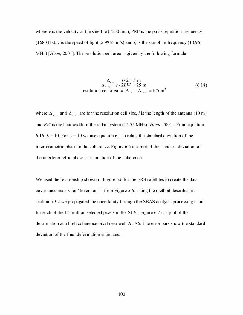
100

where v is the velocity of the satellite (7550 m/s), PRF is the pulse repetition frequency

(1680 Hz), c is the speed of light (2.99E8 m/s) and fs is the sampling frequency (18.96

MHz) [Hoen, 2001]. The resolution cell area is given by the following formula:

�

Δ a−rc = l / 2 = 5 mΔ r−rc = c / 2BW = 25 m

resolution cell area = Δ a−rc ⋅ Δ r−rc = 125 m2

(6.18)

where

�

Δ a−rc and

�

Δ a−rc are for the resolution cell size, l is the length of the antenna (10 m)

and BW is the bandwidth of the radar system (15.55 MHz) [Hoen, 2001]. From equation

6.16, L = 10. For L = 10 we use equation 6.1 to relate the standard deviation of the

interferometric phase to the coherence. Figure 6.6 is a plot of the standard deviation of

the interferometric phase as a function of the coherence.

We used the relationship shown in Figure 6.6 for the ERS satellites to create the data

covariance matrix for ‘Inversion 1’ from Figure 5.6. Using the method described in

section 6.3.2 we propagated the uncertainty through the SBAS analysis processing chain

for each of the 1.5 million selected pixels in the SLV. Figure 6.7 is a plot of the

deformation at a high coherence pixel near well ALA6. The error bars show the standard

deviation of the final deformation estimates.

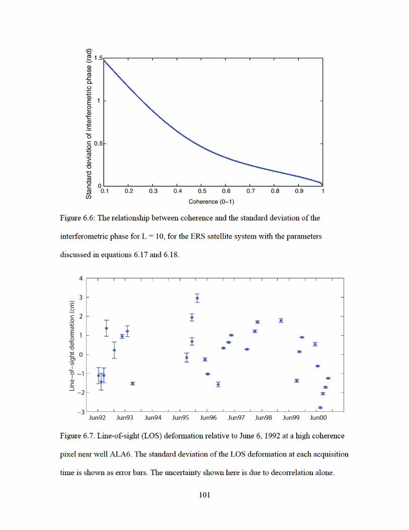
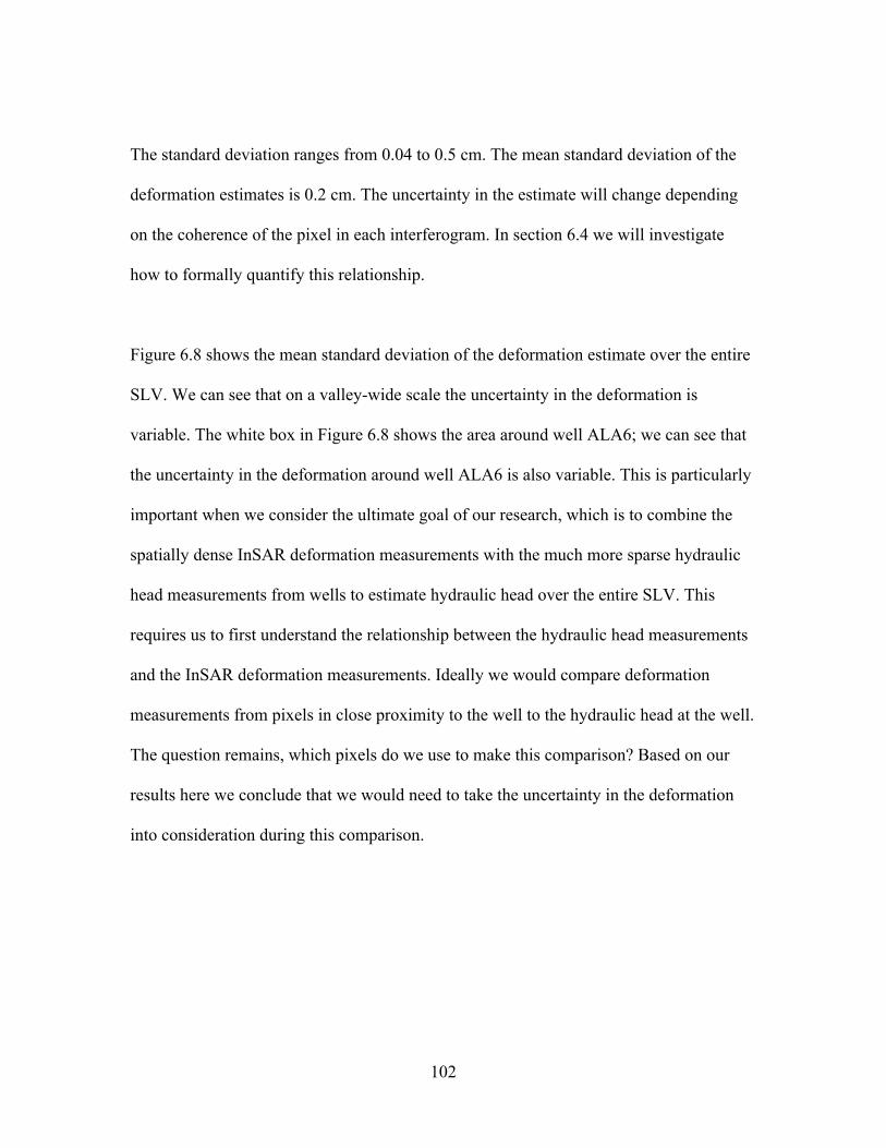
102

The standard deviation ranges from 0.04 to 0.5 cm. The mean standard deviation of the

deformation estimates is 0.2 cm. The uncertainty in the estimate will change depending

on the coherence of the pixel in each interferogram. In section 6.4 we will investigate

how to formally quantify this relationship.

Figure 6.8 shows the mean standard deviation of the deformation estimate over the entire

SLV. We can see that on a valley-wide scale the uncertainty in the deformation is

variable. The white box in Figure 6.8 shows the area around well ALA6; we can see that

the uncertainty in the deformation around well ALA6 is also variable. This is particularly

important when we consider the ultimate goal of our research, which is to combine the

spatially dense InSAR deformation measurements with the much more sparse hydraulic

head measurements from wells to estimate hydraulic head over the entire SLV. This

requires us to first understand the relationship between the hydraulic head measurements

and the InSAR deformation measurements. Ideally we would compare deformation

measurements from pixels in close proximity to the well to the hydraulic head at the well.

The question remains, which pixels do we use to make this comparison? Based on our

results here we conclude that we would need to take the uncertainty in the deformation

into consideration during this comparison.

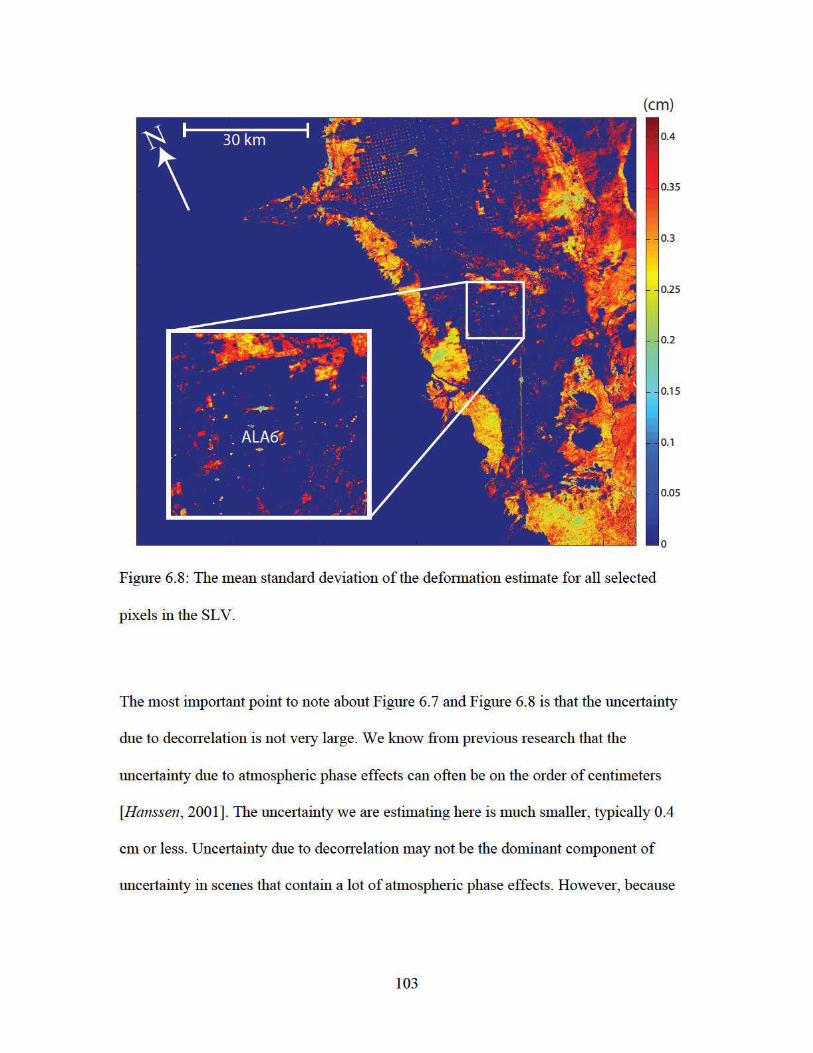
104

we do not have a way to quantify how the uncertainty due to atmospheric phase effects

varies spatially, the analysis presented in this section is still important.

6.4 Uncertainty and SBAS analysis thresholds

In the previous sections we removed scenes whose deformation measurements

were interpreted to be corrupted with atmospheric phase effects and propagated the

uncertainty due to decorrelation in the InSAR deformation measurement through the

SBAS analysis processing chain. In SBAS analysis there are a number of decision points

where we determine whether: a) there are enough interferograms, and b) the pixels have

adequate coherence. Berardino et al. (2002) required that γ > 0.26 in 50% of the

interferograms for a pixel to be selected for the processing. However, the selection of this

threshold is ad-hoc. The coherence and the uncertainty of the deformation due to

decorrelation are related, as discussed in the previous section. In this section we quantify

this relationship for our version of SBAS and the dataset in the SLV.

6.4.1 Method

We study the effects of the decision points in a controlled manner by creating a

synthetic data set. We let the time span of investigation be 8 years, the same time span as

the hydraulic head measurements at well CON2 (1992-2000), with 30 randomly selected

acquisition times. This is similar to the sampling rate for InSAR data from the ERS-1 and

ERS-2 satellites in the SLV. Each scene is assigned a randomly selected orbital position.

We apply the spatial and temporal baseline threshold to create a set of interferograms. We

vary the spatial and temporal baseline thresholds to investigate the effect of number of

105

interferograms on the uncertainty of the final deformation estimates. We next assign a

coherence value to each interferogram. The coherence values are drawn from a Gaussian

distribution, the mean and the standard deviation of which also varied. These coherence

values are used to quantify the uncertainty in the interferometric phase, which is then

propagated through the SBAS analysis processing chain to determine the uncertainty in

each deformation estimate.

6.4.2 Results and Discussion

Using the synthetic data described in section 6.4.1 we investigated the effects of

number of interferograms, mean coherence and standard deviation of the coherence on

the standard deviation of the deformation estimate. In section 6.3.3 we found that the

uncertainty in the deformation estimated at each acquisition time is different. For this

reason we created an aggregate variable for each pixel, the mean standard deviation of the

estimated deformation, which is the mean of the standard deviation for all acquisition

times.

We first investigated the relationship between the mean coherence and the mean standard

deviation of the estimated deformation while varying the number of interferograms used

in the SBAS analysis: 70 - 80, 80 - 100, 100 - 200 and 200 - 300. Figure 6.9 shows that

the number of interferograms used in our version of SBAS analysis does not appear to

greatly affect the resulting standard deviation of the deformation estimate. This implies

that changing the spatial and temporal baseline thresholds to include more interferograms

does not significantly decrease the uncertainty due to decorrelation. These results agree

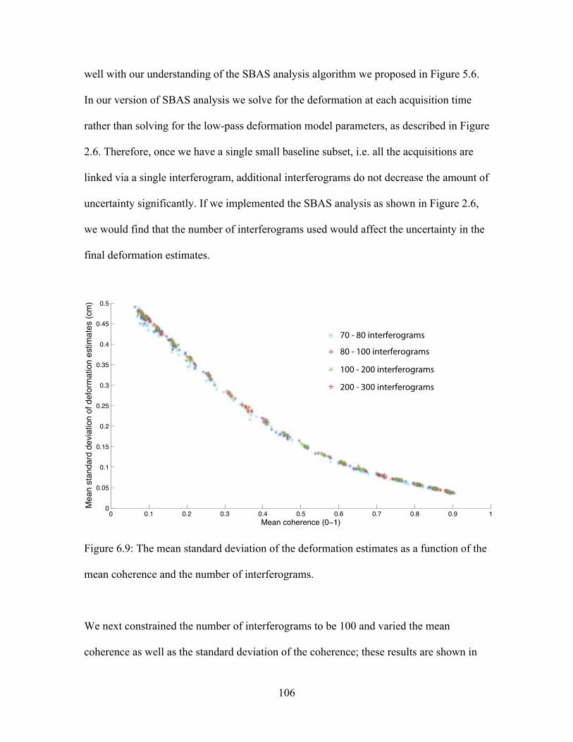
106

well with our understanding of the SBAS analysis algorithm we proposed in Figure 5.6.

In our version of SBAS analysis we solve for the deformation at each acquisition time

rather than solving for the low-pass deformation model parameters, as described in Figure

2.6. Therefore, once we have a single small baseline subset, i.e. all the acquisitions are

linked via a single interferogram, additional interferograms do not decrease the amount of

uncertainty significantly. If we implemented the SBAS analysis as shown in Figure 2.6,

we would find that the number of interferograms used would affect the uncertainty in the

final deformation estimates.

Figure 6.9: The mean standard deviation of the deformation estimates as a function of the

mean coherence and the number of interferograms.

We next constrained the number of interferograms to be 100 and varied the mean

coherence as well as the standard deviation of the coherence; these results are shown in

0 0.1 0.2 0.3 0.4 0.5 0.6 0.7 0.8 0.9 10

0.05

0.1

0.15

0.2

0.25

0.3

0.35

0.4

0.45

0.5

Mean coherence (0!1)

Mean

stan

dard

dev

iation

of d

efor

matio

n es

timat

es (c

m)

80 - 100 interferograms




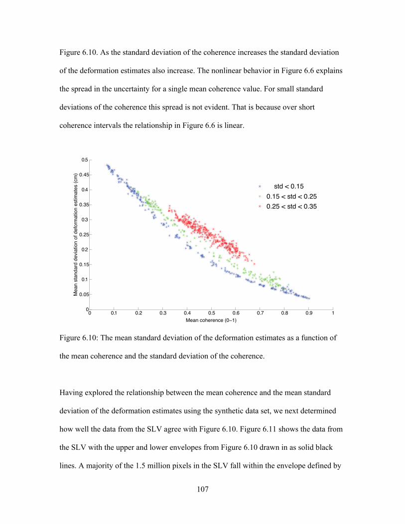
107

Figure 6.10. As the standard deviation of the coherence increases the standard deviation

of the deformation estimates also increase. The nonlinear behavior in Figure 6.6 explains

the spread in the uncertainty for a single mean coherence value. For small standard

deviations of the coherence this spread is not evident. That is because over short

coherence intervals the relationship in Figure 6.6 is linear.

Figure 6.10: The mean standard deviation of the deformation estimates as a function of

the mean coherence and the standard deviation of the coherence.

Having explored the relationship between the mean coherence and the mean standard

deviation of the deformation estimates using the synthetic data set, we next determined

how well the data from the SLV agree with Figure 6.10. Figure 6.11 shows the data from

the SLV with the upper and lower envelopes from Figure 6.10 drawn in as solid black

lines. A majority of the 1.5 million pixels in the SLV fall within the envelope defined by

0 0.1 0.2 0.3 0.4 0.5 0.6 0.7 0.8 0.9 10

0.05

0.1

0.15

0.2

0.25

0.3

0.35

0.4

0.45

0.5

Mean coherence (0!1)

Mean

stan

dard

devia

tion o

f defo

rmati

on es

timate

s (cm

)

std < 0.15

0.25 < std < 0.350.15 < std < 0.25

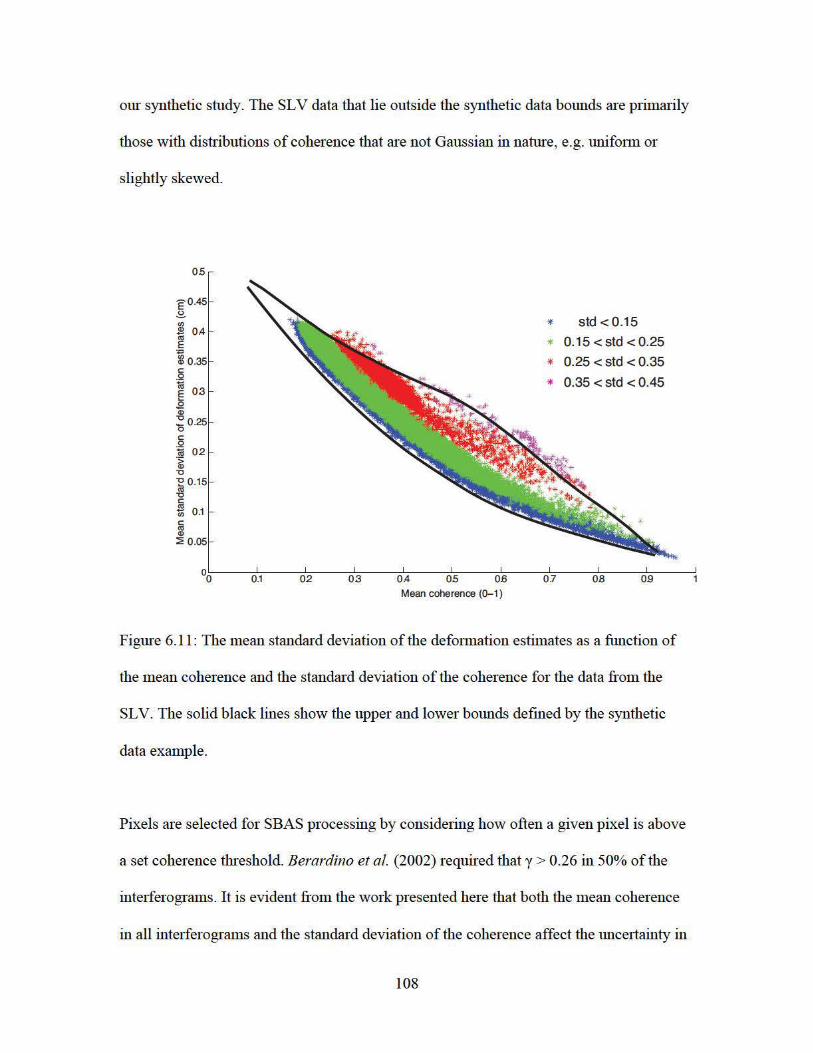
109

the deformation estimate, both in the synthetic dataset and in the data from the SLV. If

there is some acceptable uncertainty in the final deformation estimates understanding this

relationship will allow us to set the appropriate thresholds for SBAS analysis.

6.5 Conclusions

Addressing the uncertainty of InSAR-measured deformation is critical if these data

are to be used for groundwater applications as a basis for management decisions. In the

work presented in Chapter 6 we investigated the efficacy of a novel algorithm that uses

supplementary hydrologic data to identify scenes whose phase measurements may have

been corrupted with atmospheric phase effects. We also quantified the uncertainty in the

InSAR deformation measurement due to decorrelation of radar signals.

When InSAR deformation measurements are being used for a specific application, we

have shown how to set SBAS analysis thresholds in order to achieve an acceptable level

of uncertainty (section 6.4). More specifically, we determined that the number of

interferograms does not have a large effect on the uncertainty of the InSAR deformation

measurements for our version of SBAS analysis used on the data from the SLV. This

means that if researchers are evaluating possible study areas to apply our version of

SBAS analysis they should consider that the number of interferograms available would

not greatly affect the uncertainty in their final results. We also quantified the relationship

between the mean coherence, the standard deviation of the coherence and the standard

deviation of the estimated deformation. For example, if the mean coherence of a pixel is

0.5 and the standard deviation of the mean coherence is 0.25 then the uncertainty in the

110

deformation estimate will be somewhere between 0.21 cm – 0.27 cm. These results will

allow researchers to estimate the uncertainty of a dataset before performing all of the

SBAS analysis processing steps.

In section 6.3 we showed how to propagate the uncertainty due to decorrelation through

the InSAR processing chain. We now have an estimate of the uncertainty in the

deformation on a pixel-by-pixel basis. In future work, when we are comparing the

deformation and hydraulic head datasets, we will be able to compare the two based on a)

the distance from the deformation measurement to the well and b) the uncertainty in the

deformation measurement. Although it was important that we investigate how the

uncertainty due to decorrelation varies spatially, we determined that this component is

small compared to the possible uncertainty due to atmospheric phase effects.

Given the possible magnitude of the uncertainty due to atmospheric phase effects we

needed a practical solution for our specific application. In section 6.2 we showed that the

algorithm developed to identify pixels affected by atmospheric phase effects works well

with synthetic data. However, a tradeoff exists between data quality and data sampling

when being applied to real datasets. We were not able to directly evaluate the

performance of our algorithm because no other deformation measurements have been

made in the SLV during this time period.

We note that our algorithm for reducing atmospheric effects can be modified and applied

to aquifer systems that contain producing clay sediments. In our analysis we considered

111

only a linear relationship between the hydraulic head and the deformation. However, if

the hydraulic head change in the aquifer system caused changes in hydraulic head in

underlying or overlying units that contain clay, there would be some delay between the

change in hydraulic head and the deformation. In order to overcome this issue one would

first identify the periodicity of the two datasets, to determine if there is a delay. If so, one

would need to correct for it before applying our algorithm.

The algorithm as presented here is limited by the fact that we can only apply it to the

deformation time-series at pixels around the well where we have hydraulic head

measurements. However, because our algorithm only requires trends in the hydrologic

data we can use pumping data instead of, or in addition to, the hydraulic head

measurements. Pumping rates can indicate times of year that the ground surface should

be moving downward. This is especially important, as hydraulic head measurements are

often not reported to groundwater management agencies, while the reporting of well

pumping rates is becoming more common.

In Chapter 6 we showed the value of quantifying the spatially variable uncertainty in the

InSAR deformation measurements if these data are to be applied to groundwater

problems. In the chapter to follow we will use these uncertainty estimates to better

understand the relationship between deformation and hydraulic head across the entire

SLV.

112

Chapter 7

Improved estimates of hydraulic head

7.1 Introduction

In this chapter we explore ways in which the relationship between InSAR

measured deformation and measurements of hydraulic head can be utilized to increase the

spatial and temporal density of hydraulic head measurements in the confined aquifer

system of the San Luis Valley (SLV), Colorado. In Chapter 5 the relationship between

the InSAR measured deformation and hydraulic head was investigated at three well

locations. We found that the two datasets showed similar seasonality. The hydraulic head

values, derived from InSAR measured deformation and skeletal elastic storage estimates

from nearby aquifer tests, agreed with measured hydraulic head values 67% of the time.

However, the uncertainty in the InSAR derived values was on the order of meters, which

is too large for these values to be useful for groundwater applications. The uncertainty is

caused by uncertainty in the InSAR deformation measurements and the skeletal elastic

storage estimates. This led to the work in Chapter 6 where the uncertainty in the

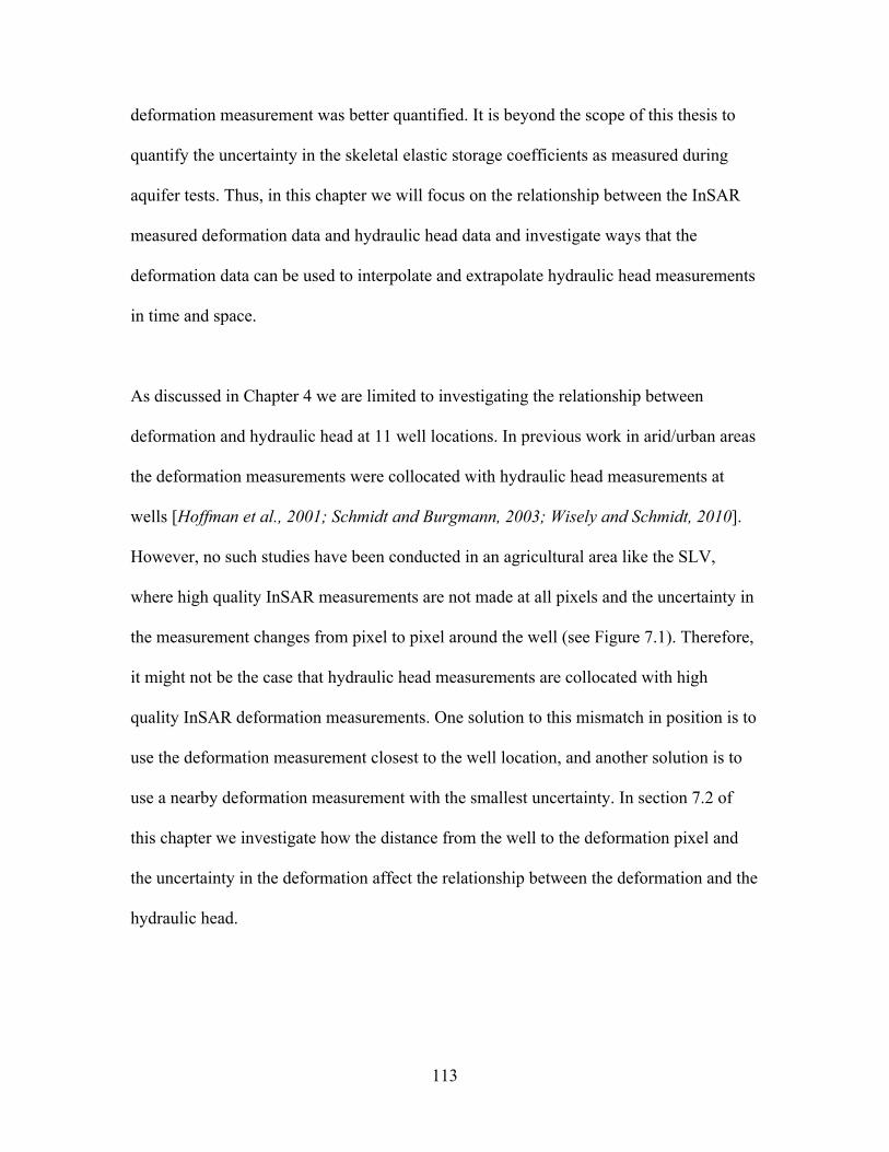
113

deformation measurement was better quantified. It is beyond the scope of this thesis to

quantify the uncertainty in the skeletal elastic storage coefficients as measured during

aquifer tests. Thus, in this chapter we will focus on the relationship between the InSAR

measured deformation data and hydraulic head data and investigate ways that the

deformation data can be used to interpolate and extrapolate hydraulic head measurements

in time and space.

As discussed in Chapter 4 we are limited to investigating the relationship between

deformation and hydraulic head at 11 well locations. In previous work in arid/urban areas

the deformation measurements were collocated with hydraulic head measurements at

wells [Hoffman et al., 2001; Schmidt and Burgmann, 2003; Wisely and Schmidt, 2010].

However, no such studies have been conducted in an agricultural area like the SLV,

where high quality InSAR measurements are not made at all pixels and the uncertainty in

the measurement changes from pixel to pixel around the well (see Figure 7.1). Therefore,

it might not be the case that hydraulic head measurements are collocated with high

quality InSAR deformation measurements. One solution to this mismatch in position is to

use the deformation measurement closest to the well location, and another solution is to

use a nearby deformation measurement with the smallest uncertainty. In section 7.2 of

this chapter we investigate how the distance from the well to the deformation pixel and

the uncertainty in the deformation affect the relationship between the deformation and the

hydraulic head.

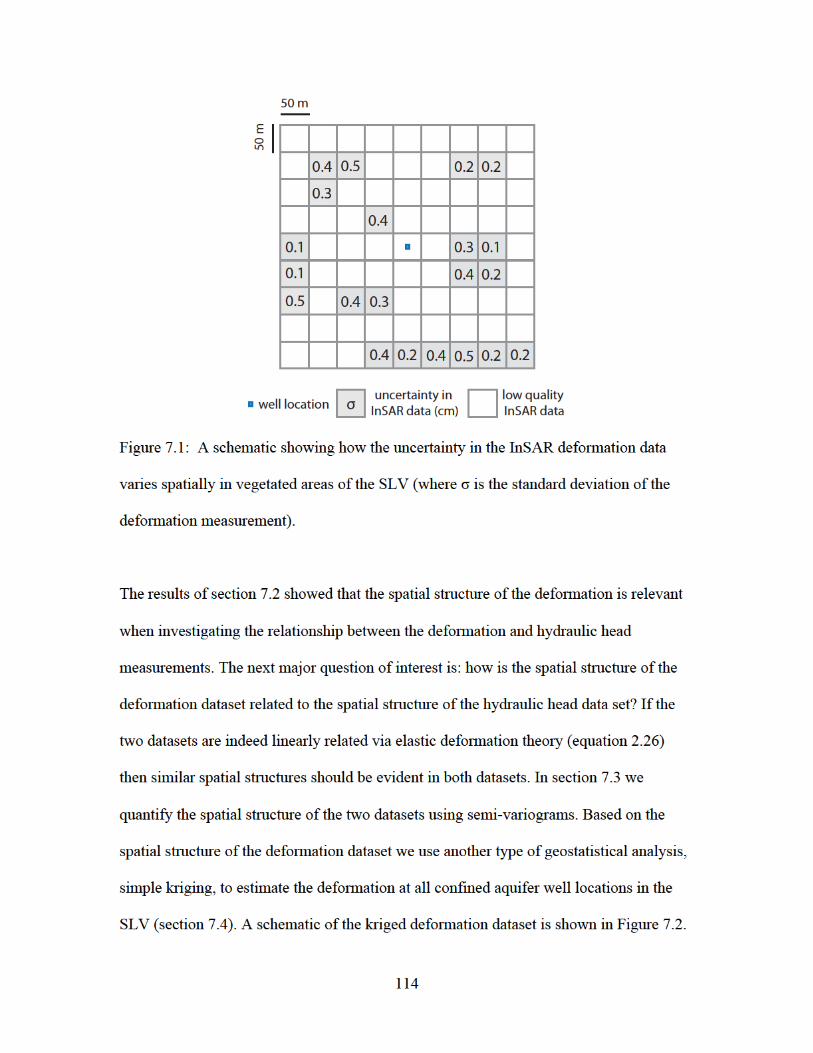
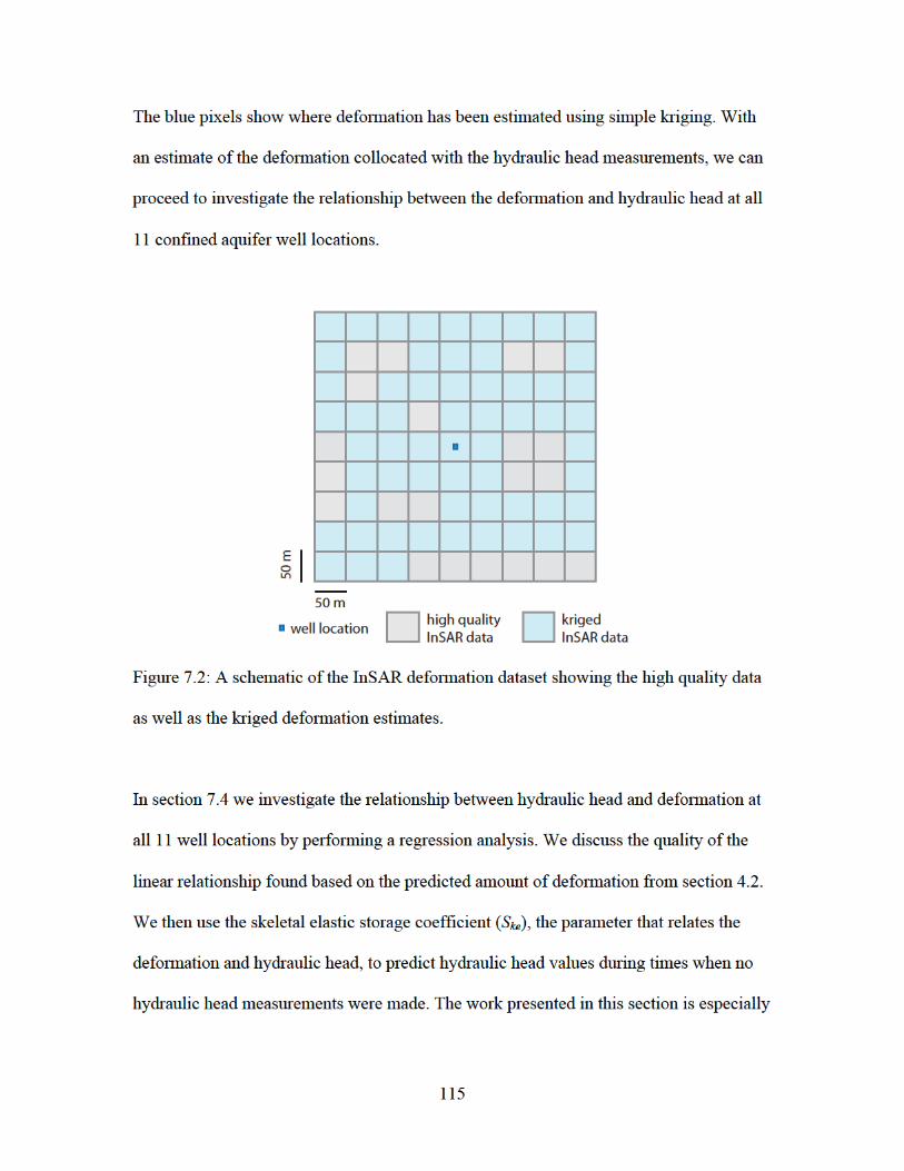
116

relevant for agricultural areas where temporal gaps in hydraulic head time series can be

estimated using InSAR deformation data.

We begin this chapter by investigating the relationship between the hydraulic head and

the deformation for a number of pixels around specific well locations (Section 7.2). This

works leads to the comparison of the spatial structures of the deformation dataset and the

hydraulic head dataset (Section 7.3). Once we understand how the deformation dataset

varies spatially we use simple kriging to estimate the deformation directly at confined

aquifer well locations. This allows us to determine the relationship between the hydraulic

head measurements and deformation measurements at the well locations and predict

hydraulic head back in time using the estimates of Ske (section 7.4).

7.2 The relationship between head and deformation around three wells

The first step towards understanding the relationship between InSAR deformation

measurements and hydraulic head measurements is to investigate how this relationship

varies from pixel to pixel around a single well (see Figure 7.1). In this section we

compare the deformation and head datasets at three well locations: ALA6, ALA7 and

ALA8. These wells were selected for this initial analysis because they are all located

within the large subsidence bowl observed in a number of the raw interferograms. This

large visible deformation signal is indicative of an area with a large signal to noise ratio.

The deformation data used in this chapter is the same high quality dataset (see section

3.4) used in Chapters 5 and 6, with 31 SAR acquisitions from 1992 – 2000.

117

The work in this section assumes, a) all the deformation measured at the surface (Δd) is

indeed caused by aquifer compaction (Δb), i.e. Δb =Δd in equation 2.26, b) only elastic

deformation is occurring, i.e. no clay drainage is occurring within the confined aquifer

system or from the overlying confining unit. Given these assumptions the two datasets

are linearly related through the skeletal elastic storage coefficient (Ske). The main

question of this section is, how does this linear relationship change for deformation

measurements made around a well? The section to follow describes the linear regression

analysis used to quantitatively assess this relationship.

7.2.1 Linear regression analysis

The linear regression analysis of the deformation and hydraulic head data takes

into account the changing uncertainty in the deformation measurements as determined in

Chapter 6 [York et al., 2004]. The uncertainty in the hydraulic head measurements is

estimated to be +/- 10 cm [Eric Harmon personal communication, 2012]. The slope of

the linear best fit, between the Δh and Δd, provides an estimate of the elastic skeletal

storage coefficient (Ske) at each pixel location within 1 km of the well. The goodness of

fit is evaluated at each pixel location by calculating the coefficient of determination ( )

using the following set of equations:

�

SStot = yi − y ( )2i∑

SSerr = yi − ˆ y ( )2i∑

R2 ≡1− SSerr

SStot

, (7.1)

€

R2

118

where y is the dependent variable (the deformation as measured by InSAR), is the

mean value of the dependent variable and is the estimated value of the dependent

variable given the regression parameters. is the total sum of squares and is the

residual sum of squares. In the sections to follow we will investigate first how the

estimate of Ske varies spatially around the wells, and then how the average uncertainty in

the InSAR deformation measurement affects the goodness of fit between deformation and

hydraulic head.

7.2.2 Variability of Ske around wells: ALA6, ALA7 and ALA8

Figure 7.3 shows the spatial distribution of Ske estimates around the wells at the

locations of the high quality deformation measurements. The spatial patterns seen Figure

7.3 are solely a product of the location of the high quality deformation measurements as

determined in section 5.4. The axes of latitude and longitude in each plot have slightly

different scales, and it should be noted that neighboring pixels are approximately 50 m

apart. Ske varies from 0.0034 – 0.0086, which are reasonable values for the sediments

found in the aquifer system in the SLV. We can see that Ske is more variable around well

ALA7 (0.0057 – 0.0085), than around ALA6 (0.0031 – 0.0047) and ALA8 (0.0055 –

0.0068).

€

y

€

ˆ y

€

SStot

€

SSerr

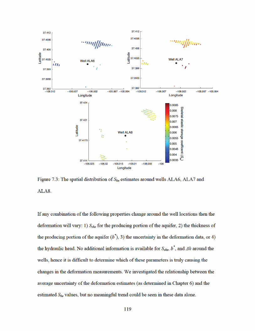
120

7.2.3 Average uncertainty in the InSAR deformation measurements and R2

In this section we investigate how the average uncertainty of the deformation

estimates (as estimated in Chapter 6) affect the linear relationship between the InSAR

measured deformation and hydraulic head. The goodness of fit parameter (R2) was used

to quantify the linearity of the relationship. The left plot in Figure 7.4 shows R2 as a

function of distance from the pixel to well ALA6, and the right hand plot shows a plan

view of the pixels around well ALA6. The colors define the average uncertainty of the

deformation estimates at a given pixel, where red is low uncertainty and blue is high

uncertainty. It is clear that at this well location the pixels closest to the well provide the

best fit between the deformation data and the hydraulic head data, regardless of the

uncertainty in the deformation measurements. However, no simple relationship can be

drawn from the plots in Figures 7.4 to link R2 with the average uncertainty of the

deformation measurements.

Figure 7.5 shows the same plots for well ALA7. However, at this well location the

regression of Δh and Δd at the pixels closest to the well do not produce the highest R2

values. In fact, 90% of the regressions around well ALA7 produce R2 values between 0.8

and 0.86. At this well location the pixels proximity to the well does not appear to

systematically affect the linear relationship between Δh and Δd, contrary to what was

observed at well ALA6. Similarly to ALA6, no simple relationship can be drawn between

the distance from the pixel to the well, the uncertainty and R2 (see Figure 7.5).

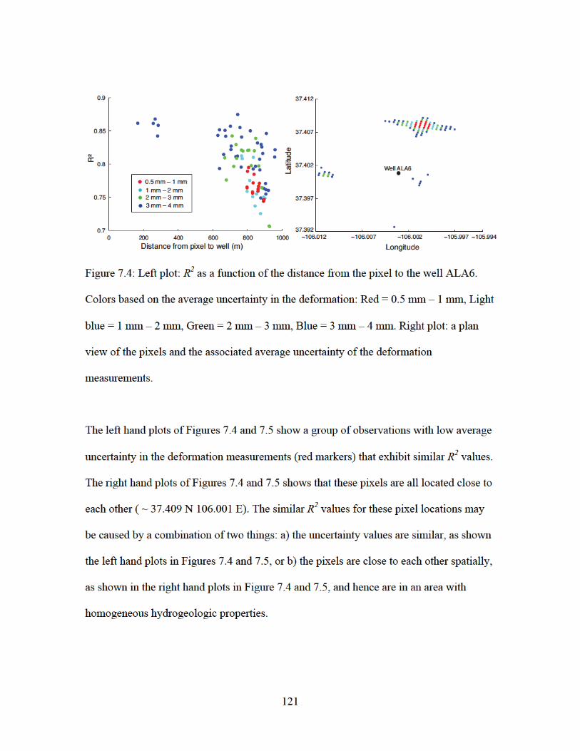
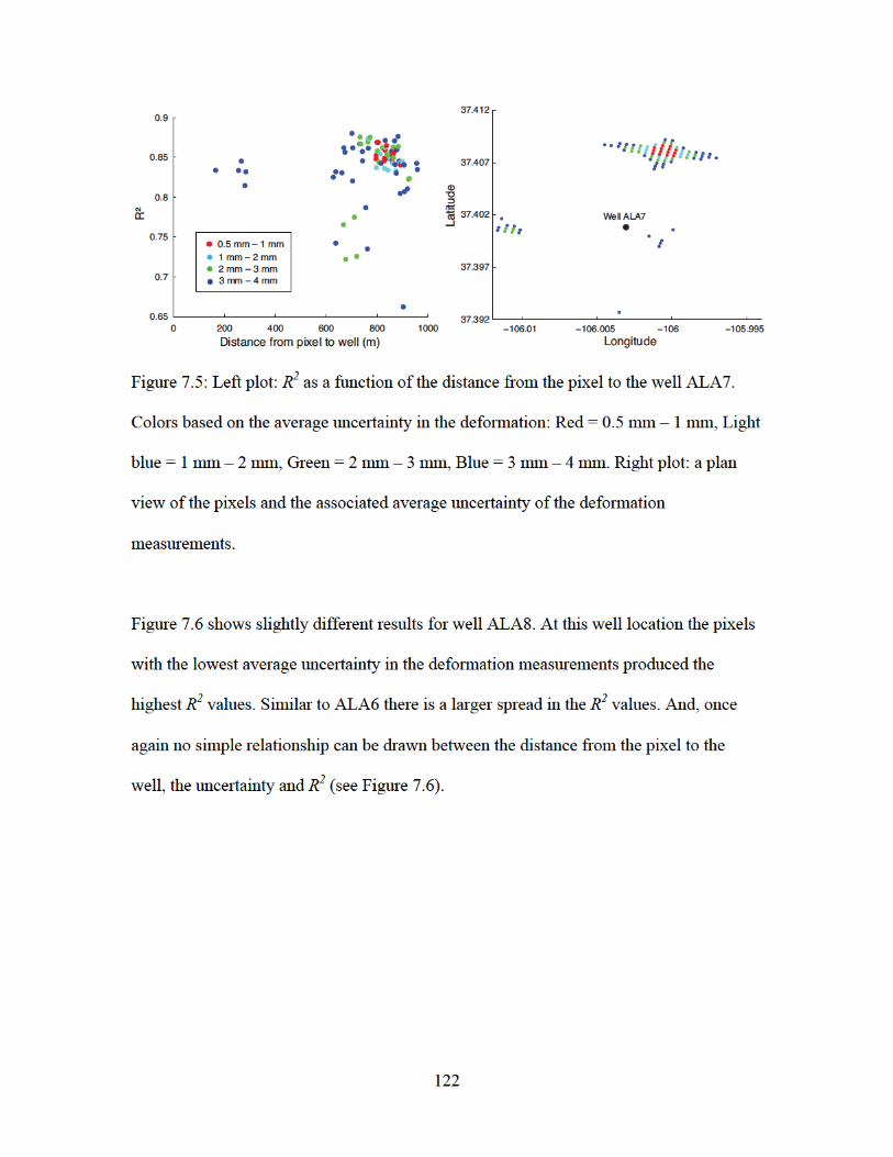
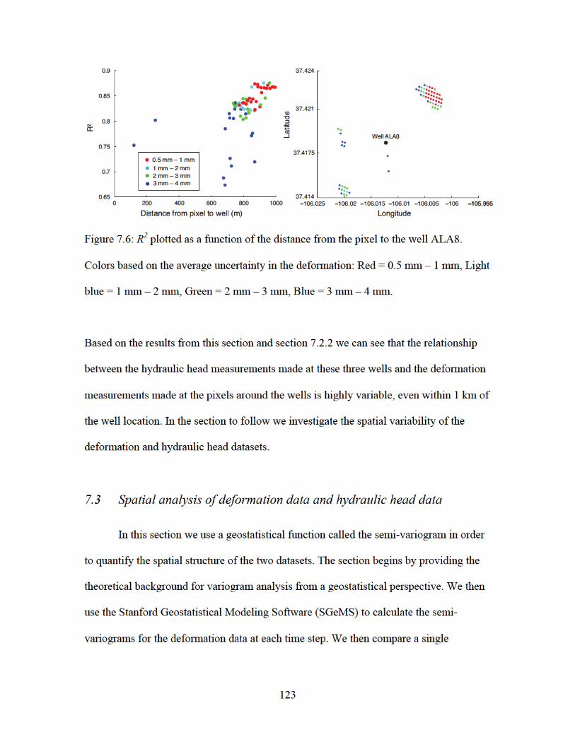
124

deformation semi-variogram to the hydraulic head semi-variogram from the same time

period in order to investigate the spatial similarities of the two datasets.

7.3.1 Geostatistical definition of the variogram

The main geostatistical calculation that we use in this section is known as the

semi-variogram (γ). For some random variable z at some spatial location u, the semi-

variogram is an average of the squared differences of the variable at location u to location

u plus some lag vector h. If we calculate the semi-variogram for all lag distances then we

have the following formula:

, (7.2)

where N is the number of measurement pairs with a given lag distance h. The semi-

variogram is a measure of the average dissimilarity of a random variable at specific lag

distances. It is important to note that this definition is appropriate when the data are

equally spaced. However, when the data are irregularly spaced or sparse, it becomes

important to include what is known as a lag tolerance. This means that lag distances plus

or minus the tolerance are averaged together. If the direction of the lag vector is not

considered in the calculation then the semi-variogram is called omni-directional.

If some anisotropy is expected in the spatial data then directional semi-variograms should

be calculated. For practical purposes directional variograms are usually calculated with

€

γ(h) =12N

z(ui + h) − z(ui )[ ]2i=1

N

∑

125

some angular tolerance for the lag vector. If the directional variogram is calculated for all

angles from 0 – 180 degrees then we can create what is known as a 2D variogram map.

The directional variograms are plotted on a color scale along the angle of the lag vector.

The variability in the color for a set lag distance across all angles can highlight important

anisotropic spatial structures.

When analyzing semi-variograms it is often useful to fit the different structures in the

semi-variogram with different models. In doing so, semi-variograms can be compared

quantitatively. In the work completed in the following section we either use an

exponential model or a linear model to characterize the different structures observed. The

exponential model has the following form:

, (7.3)

and is characterized by the sill (c), the range (a), and the nugget (n). Figure 7.7 shows a

schematic of an exponential semi-variogram model. For longer lag distances the

exponential semi-variogram model levels out, the semi-variogram value where this

occurs is called the sill. The lag distance where the semi-variogram model reaches 95%

of the sill value is known as the range. The range describes the scale at which the two

measurements of the variable become practically uncorrelated and provides an intrinsic

correlation length. Theoretically the semi-variogram value at the origin should be zero.

But, because of random observation error and variability below the sampling scale of the

€

γ(h) = (c × (1 - exp-ha

$

% &

'

( ) )) + n

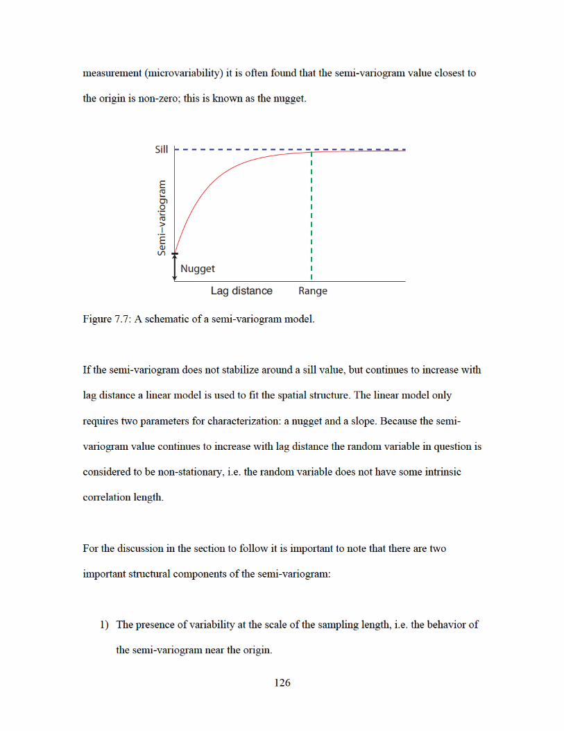
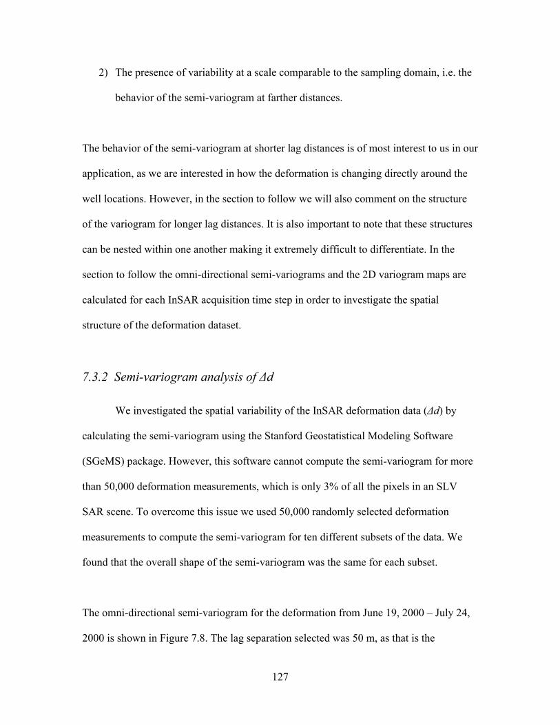
127

2) The presence of variability at a scale comparable to the sampling domain, i.e. the

behavior of the semi-variogram at farther distances.

The behavior of the semi-variogram at shorter lag distances is of most interest to us in our

application, as we are interested in how the deformation is changing directly around the

well locations. However, in the section to follow we will also comment on the structure

of the variogram for longer lag distances. It is also important to note that these structures

can be nested within one another making it extremely difficult to differentiate. In the

section to follow the omni-directional semi-variograms and the 2D variogram maps are

calculated for each InSAR acquisition time step in order to investigate the spatial

structure of the deformation dataset.

7.3.2 Semi-variogram analysis of Δd

We investigated the spatial variability of the InSAR deformation data (Δd) by

calculating the semi-variogram using the Stanford Geostatistical Modeling Software

(SGeMS) package. However, this software cannot compute the semi-variogram for more

than 50,000 deformation measurements, which is only 3% of all the pixels in an SLV

SAR scene. To overcome this issue we used 50,000 randomly selected deformation

measurements to compute the semi-variogram for ten different subsets of the data. We

found that the overall shape of the semi-variogram was the same for each subset.

The omni-directional semi-variogram for the deformation from June 19, 2000 – July 24,

2000 is shown in Figure 7.8. The lag separation selected was 50 m, as that is the

128

approximate distance between pixel centers. To accommodate variability in the distance

between pixel centers a tolerance of 5 m was included in the calculation. The semi-

variogram value at the first lag calculation is not at the origin; this indicates that the data

either contain some microvariability or significant uncertainty. The semi-variogram

shows a nested structure: for lag distances up to 1850 m the data appear to fit an

exponential model (shown as a red line), and for lag distances greater than 1850 m the

semi-variogram shows a linear structure. The short length scale structure is particularly

important as it helps us understand how the deformation is varying around specific well

locations. If we assume that the deformation and the change in hydraulic head are linearly

related then on average the changes in hydraulic head that are more than ~ 2 km apart are

also not spatially related to one another.

Figure 7.8: Experimental variogram for lag spacing 50 m, and tolerance 5 m. The red line

shows a schematic of an exponential variogram model.

0 5 10 15 20 250

0.05

0.1

0.15

0.2

0.25

0.3

0.35

Lag distance (km)

Semi

-vario

gram

semi-variogramexponential model

129

This result in itself has large implications for the way that the hydraulic head data are

being used in the SLV. As discussed in Chapter 1 the Rio Grande Decision Support

System (RGDSS) uses a MODFLOW groundwater flow model to predict hydraulic head

change given certain pumping and recharge conditions for the confined aquifer system.

However there are not sufficient observations of hydraulic head for the model to properly

calibrate. In the model the confined aquifer system is made up of three hydrogeologic

layers that are designed as continuous layers with specific boundary conditions set by

estimated recharge rates around the rim of the SLV. Given the continuous layer model

one expects the changes in hydraulic head to be related over large distances, whereas here

the deformation data infer that the changes in hydraulic head are not related over large

distances.

Another important note to make about the semi-variogram of the deformation data in

Figure 7.8, is that the deformation data may still contain a large amount of uncertainty

due to atmospheric phase effects. We are not able to ameliorate this uncertainty, as in

many other studies implementing SBAS analysis, because of the nature of the hydraulic

head time-series in the SLV (see Figure 5.5 in Section 5.5). Because we observe a nested

structure in the semi-variogram in Figure 7.8, it may be possible that one of those

structures is caused by the deformation and the other is caused by the uncertainty due to

atmospheric phase effects. Note that the variogram is often referred to as a structure

function in this field of study. Theoretical studies have estimated the shape of the

structure function based on specific atmospheric parameters for sites in the mid-latitudes

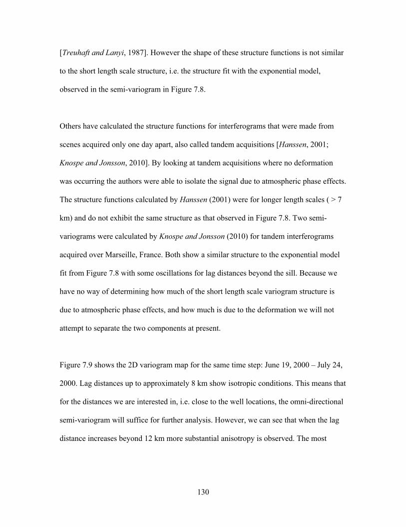
130

[Treuhaft and Lanyi, 1987]. However the shape of these structure functions is not similar

to the short length scale structure, i.e. the structure fit with the exponential model,

observed in the semi-variogram in Figure 7.8.

Others have calculated the structure functions for interferograms that were made from

scenes acquired only one day apart, also called tandem acquisitions [Hanssen, 2001;

Knospe and Jonsson, 2010]. By looking at tandem acquisitions where no deformation

was occurring the authors were able to isolate the signal due to atmospheric phase effects.

The structure functions calculated by Hanssen (2001) were for longer length scales ( > 7

km) and do not exhibit the same structure as that observed in Figure 7.8. Two semi-

variograms were calculated by Knospe and Jonsson (2010) for tandem interferograms

acquired over Marseille, France. Both show a similar structure to the exponential model

fit from Figure 7.8 with some oscillations for lag distances beyond the sill. Because we

have no way of determining how much of the short length scale variogram structure is

due to atmospheric phase effects, and how much is due to the deformation we will not

attempt to separate the two components at present.

Figure 7.9 shows the 2D variogram map for the same time step: June 19, 2000 – July 24,

2000. Lag distances up to approximately 8 km show isotropic conditions. This means that

for the distances we are interested in, i.e. close to the well locations, the omni-directional

semi-variogram will suffice for further analysis. However, we can see that when the lag

distance increases beyond 12 km more substantial anisotropy is observed. The most

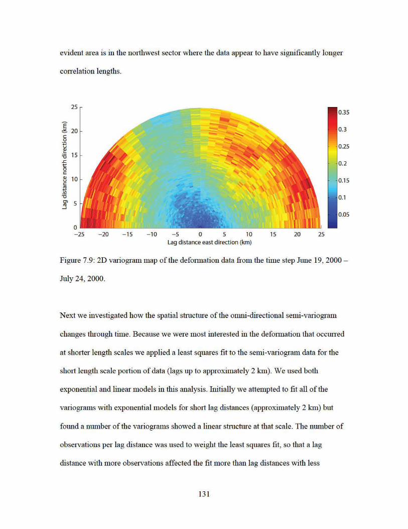
132

observations. The semi-variograms for all the acquisition times are shown in Figures 7.10

– 7.13.

The structure of these variograms changes significantly from one acquisition time to the

next. We fit four of the variograms with linear models, and 26 with exponential models.

The exponential models show a lot of variability in the best-fit parameters. The mean

range for the variograms fit with an exponential model was 3.9 km, with a standard

deviation of 2.5 km. This implies that the deformation estimates vary spatially on a

number of different length scales, which is dependent on the surface deformation and the

atmospheric conditions at that acquisition time. The mean nugget equals 0.0253, with a

standard deviation of 0.0221. This indicates that a lot of variability exists in either: a) the

microvariability of the data, or b) the uncertainty from one acquisition time to the next.

Since we have already observed that the uncertainty in the deformation data changes from

one acquisition time to the next due to changes in coherence (see Chapter 5), this is the

most likely source for the variability in the size of the nugget. In the next section we

proceed with an analysis of the spatial variability of the hydraulic head data.

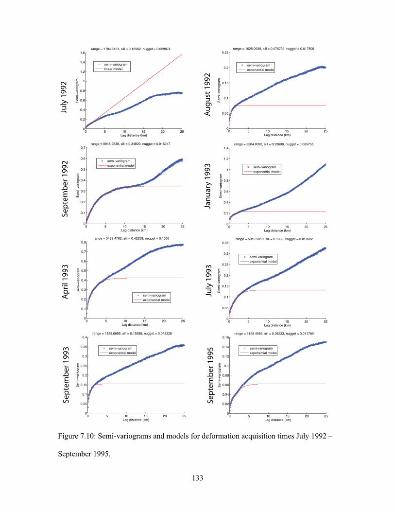
133

Figure 7.10: Semi-variograms and models for deformation acquisition times July 1992 –

September 1995.

0 5 10 15 20 250

0.2

0.4

0.6

0.8

1

1.2

1.4

1.6

Lag distance (km)

Semi

!var

iogra

m

range = 1784.5161, sill = 0.10982, nugget = 0.029874

semi-variogramlinear model

0 5 10 15 20 250

0.05

0.1

0.15

0.2

0.25

Lag distance (km)

Semi

!var

iogra

m



0 5 10 15 20 250

0.1

0.2

0.3

0.4

0.5

0.6

0.7

Lag distance (km)

Semi

!var

iogra

m


0 5 10 15 20 250

0.2

0.4

0.6

0.8

1

1.2

1.4

Lag distance (km)

Semi

!var

iogra

m


0 5 10 15 20 250

0.1

0.2

0.3

0.4

0.5

0.6

0.7

0.8

Lag distance (km)

Semi

!var

iogra

m


0 5 10 15 20 250

0.05

0.1

0.15

0.2

0.25

0.3

0.35

Lag distance (km)

Semi

!var

iogra

m


0 5 10 15 20 250

0.05

0.1

0.15

0.2

0.25

0.3

0.35

0.4

Lag distance (km)

Semi

!var

iogra

m


0 5 10 15 20 250

0.02

0.04

0.06

0.08

0.1

0.12

0.14

0.16

Lag distance (km)

Semi

!var

iogra

m


July

199

2

Augu

st 1

992

Janu

ary

1993

Sept

embe

r 199

2

July

199

3

April

199

3

Sept

embe

r 199

5

Sept

embe

r 199

3







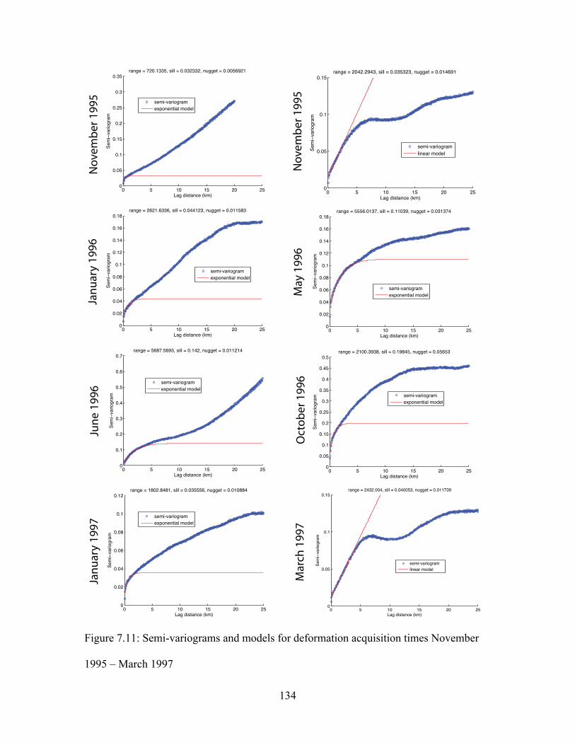
134

Figure 7.11: Semi-variograms and models for deformation acquisition times November

1995 – March 1997

0 5 10 15 20 250

0.05

0.1

0.15

0.2

0.25

0.3

0.35

Lag distance (km)

Semi

!var

iogra

m


0 5 10 15 20 250

0.05

0.1

0.15

Lag distance (km)

Semi

!var

iogra

m



0 5 10 15 20 250

0.02

0.04

0.06

0.08

0.1

0.12

0.14

0.16

0.18

Lag distance (km)

Semi

!var

iogra

m


0 5 10 15 20 250

0.02

0.04

0.06

0.08

0.1

0.12

0.14

0.16

0.18

Lag distance (km)

Semi

!var

iogra

m


0 5 10 15 20 250

0.1

0.2

0.3

0.4

0.5

0.6

0.7

Lag distance (km)

Semi

!var

iogra

m


0 5 10 15 20 250

0.05

0.1

0.15

0.2

0.25

0.3

0.35

0.4

0.45

0.5

Lag distance (km)

Semi

!var

iogra

m


0 5 10 15 20 250

0.02

0.04

0.06

0.08

0.1

0.12

Lag distance (km)

Semi

!var

iogra

m


0 5 10 15 20 250

0.05

0.1

0.15

Lag distance (km)

Sem

i!var

iogra

m



Mar

ch 1

997

Janu

ary

1997

Oct

ober

199

6

June

199

6

May

199

6

Janu

ary

1996

Nov

embe

r 199

5

Nov

embe

r 199

5 semi-variogramexponential model






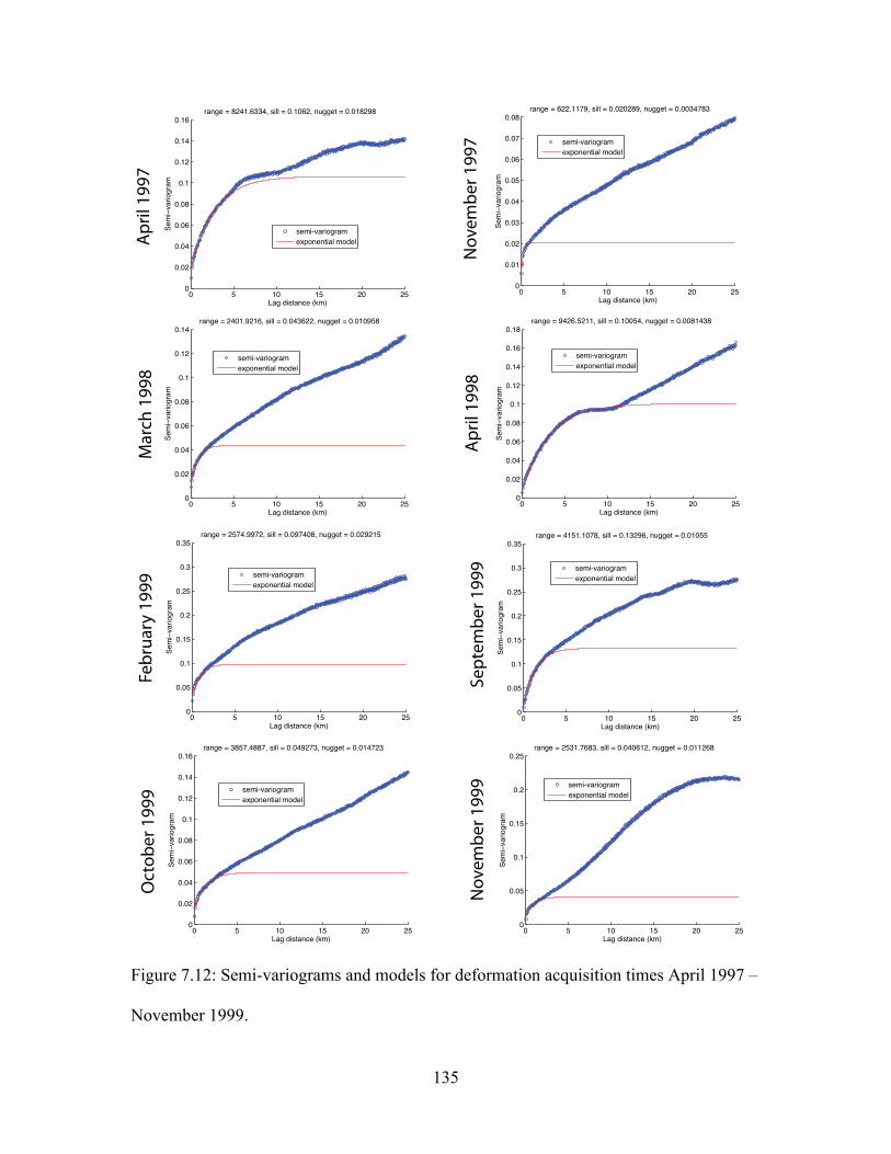
135

Figure 7.12: Semi-variograms and models for deformation acquisition times April 1997 –

November 1999.

0 5 10 15 20 250

0.01

0.02

0.03

0.04

0.05

0.06

0.07

0.08

Lag distance (km)

Semi

!var

iogra

m


0 5 10 15 20 250

0.02

0.04

0.06

0.08

0.1

0.12

0.14

0.16

Lag distance (km)

Semi

!var

iogra

m


0 5 10 15 20 250

0.02

0.04

0.06

0.08

0.1

0.12

0.14

Lag distance (km)

Semi

!var

iogra

m


0 5 10 15 20 250

0.02

0.04

0.06

0.08

0.1

0.12

0.14

0.16

0.18

Lag distance (km)Se

mi!v

ariog

ram


0 5 10 15 20 250

0.05

0.1

0.15

0.2

0.25

0.3

0.35

Lag distance (km)

Semi

!var

iogra

m


0 5 10 15 20 250

0.05

0.1

0.15

0.2

0.25

0.3

0.35

Lag distance (km)

Semi

!var

iogra

m


0 5 10 15 20 250

0.02

0.04

0.06

0.08

0.1

0.12

0.14

0.16

Lag distance (km)

Semi

!var

iogra

m


0 5 10 15 20 250

0.05

0.1

0.15

0.2

0.25

Lag distance (km)

Semi

!var

iogra

m


April

199

7

Nov

embe

r 199

7

Mar

ch 1

998

April

199

8

Febr

uary

199

9

Sept

embe

r 199

9

Oct

ober

199

9

Nov

embe

r 199

9







semi-variogramexponential modelsemi-variogram

exponential model

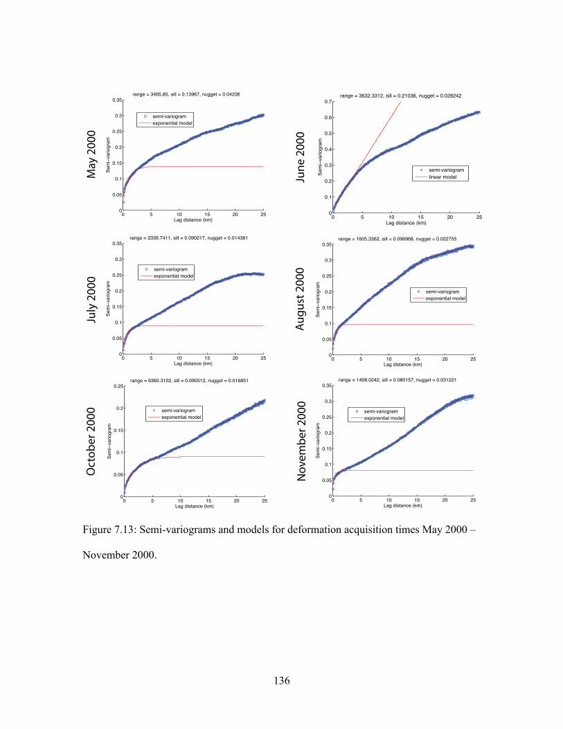
136

Figure 7.13: Semi-variograms and models for deformation acquisition times May 2000 –

November 2000.

0 5 10 15 20 250

0.05

0.1

0.15

0.2

0.25

0.3

0.35

Lag distance (km)

Semi

!var

iogra

m


0 5 10 15 20 250

0.1

0.2

0.3

0.4

0.5

0.6

0.7

Lag distance (km)

Semi

!var

iogra

m



0 5 10 15 20 250

0.05

0.1

0.15

0.2

0.25

0.3

0.35

Lag distance (km)

Semi

!var

iogra

m


0 5 10 15 20 250

0.05

0.1

0.15

0.2

0.25

0.3

0.35

Lag distance (km)

Semi

!var

iogra

m


0 5 10 15 20 250

0.05

0.1

0.15

0.2

0.25

Lag distance (km)

Semi

!var

iogra

m


0 5 10 15 20 250

0.05

0.1

0.15

0.2

0.25

0.3

0.35

Lag distance (km)

Semi

!var

iogra

m


May

200

0

June

200

0

July

200

0

Augu

st 2

000

Oct

ober

200

0

Nov

embe

r 200

0






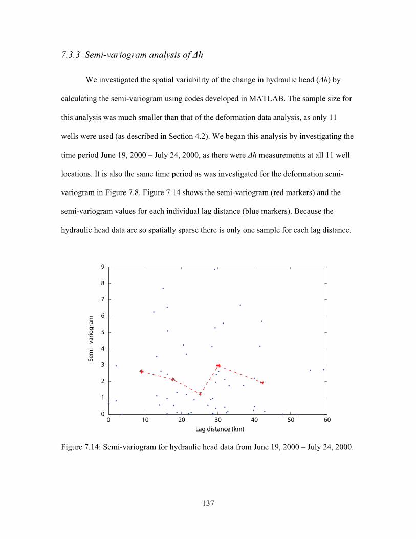
137

7.3.3 Semi-variogram analysis of Δh

We investigated the spatial variability of the change in hydraulic head (Δh) by

calculating the semi-variogram using codes developed in MATLAB. The sample size for

this analysis was much smaller than that of the deformation data analysis, as only 11

wells were used (as described in Section 4.2). We began this analysis by investigating the

time period June 19, 2000 – July 24, 2000, as there were Δh measurements at all 11 well

locations. It is also the same time period as was investigated for the deformation semi-

variogram in Figure 7.8. Figure 7.14 shows the semi-variogram (red markers) and the

semi-variogram values for each individual lag distance (blue markers). Because the

hydraulic head data are so spatially sparse there is only one sample for each lag distance.

Figure 7.14: Semi-variogram for hydraulic head data from June 19, 2000 – July 24, 2000.

0 10 20 30 40 50 600

1

2

3

4

5

6

7

8

9

Sem

i!va

riogr

am

Lag distance (km)

138

The semi-variogram in Figure 7.14 shows no distinct trend to suggest any specific spatial

structure. Often variograms of hydraulic head data fit a quadratic model, such that wells

close together show very similar hydraulic head values over some distinct distance

[Kitanidis, 1997]. There is no evidence of this typical quadratic structure in this dataset. It

is important to note that variograms are aimed at capturing the average spatial structure of

a set of measurements. In this instance, only 11 measurements were available over large

spatial scales (10’s of kilometers), and hence the semi-variogram did not show any

structure that is comparable to the structures observed in the deformation data. This

highlights an inherent benefit of using InSAR deformation data for groundwater

problems; the deformation data show finer spatial structures that are often not captured by

hydraulic head data. These finer scale spatial structures contain important information

about how the hydraulic head or subsurface geology is changing spatially. However, it

also shows an inherent drawback to the analysis in the SLV; the deformation data need to

be validated by the hydraulic head data that has a much lower spatial resolution. Because

of this low spatial resolution, as seen in the semi-variogram in Figure 7.14, it is

impossible to make a comparison of the spatial structure of these two datasets.

7.4 Comparison of hydraulic head data and deformation data at wells

The spatial variability of the deformation dataset allowed us to understand why

the relationship between the hydraulic head measured at the well and the deformation

measurements around wells ALA6, ALA7 and ALA8 was so variable. The short scale

spatial structure in the deformation dataset showed that on average the deformation

changes significantly within a 1 km radius of the wells. If we refer back to equation 2.26

139

this implies that either the hydraulic head is changing, the producing thickness is

changing,

�

Sske is changing, or that the data contain atmospheric phase effects. In this

section we will estimate the deformation directly at the well locations using the semi-

variograms calculated in the previous section and a geostatistical technique called simple

kriging.

7.4.1 Simple kriging of deformation data

SGeMS was used to perform the kriging of the deformation data. Kriging is a

form of generalized linear regression that provides an optimal spatial estimator by

minimizing the mean-squared-error between measured data and the estimated data at a

given location [Deutsch and Journel, 1992]. Semi-variogram models, which characterize

the spatial structure of the system, provide the optimal spatial estimator, which can then

be used to estimate the variable in question at locations where it is unknown. i.e. at the

well locations. In the Earth sciences many variants of kriging have been implemented,

however the most basic form is known as simple kriging. We have chosen to use simple

kriging over other more complicated forms because the technique implies that a valid

mean for the dataset can be calculated, and because the deformation dataset is spatially

dense this is a valid assumption.

Simple kriging, as implemented in SGeMS, does not incorporate the uncertainty of the

data into the kriging algorithm. However, the kriged estimate of the deformation at the

well location should be influenced by the uncertainty of the deformation at surrounding

pixels. Therefore, a stochastic technique was implemented in order to incorporate this

140

uncertainty. For a single acquisition of deformation data, at a single selected pixel

location, we randomly assigned a deformation from a Gaussian distribution. The

Gaussian distribution was created with a mean equal to deformation measurement and a

standard deviation equal to the uncertainty in the deformation measurement (as calculated

in Chapter 6). We repeated this procedure 30 times, i.e. 30 realizations of the deformation

datum. We found that the mean value of the 30 realizations was within 10% of the

measured deformation. This process was repeated for all selected pixels within 2 km of

the well location and all acquisition times. By using this method the kriged deformation

will have an associated uncertainty that is influenced by both the uncertainty in the

deformation data itself as well as the uncertainty associated with the kriging algorithm.

We applied this process to the deformation data surrounding all 11 wells.

7.4.2 Linear regression of kriged deformation data and head data

In this section we apply the same linear regression, as described in section 7.2.1,

on the hydraulic head data and the kriged deformation data at the 11 well locations. We

begin by discussing the linear regression results at the three well investigated in section

7.2: ALA6, ALA7 and ALA8. We then discuss the results of the linear regression

analysis for the remaining 8 wells .

The results of the linear regression of Δh and Δd at well ALA6 are shown in the left plot

of Figure 7.15A. The deformation and the hydraulic head appear to be linearly related at

this location (R2 = 0.875). The grey circles signify the uncertainty in the InSAR

measurement as calculated from the stochastic analysis previously described. The slope

141

of the regression line (Ske = 4.44 ×10-3 +/- 2.64 ×10-4) was then used to estimate the

hydraulic head from the deformation measurements, shown in the plot on the right. We

can see that the interpolated hydraulic head data are within the error bars of the estimated

hydraulic head data 40% of the time (right plot Figure 7.15A). The uncertainty in the

hydraulic head estimates is approximately +/- 0.5 m, which is much less than the

uncertainty in the hydraulic head estimate from Chapter 5 (+/- 5 m at ALA6) when

aquifer test parameters were used. As discussed in Chapter 5 an aquifer test was

performed 300 m away from well ALA6 which resulted in an estimate of S = 1.4 ×10-3

+/- 2.8 ×10-4. If we assume that S is a proxy for Ske, i.e. the storage change due to the

expansion and contraction of water is small (Sw), then we can compare these two results.

We find that Ske from the regression analysis is larger than S from the aquifer test. This

could be due to a number of factors, e.g. uncertainty in the depth of the producing zone,

spatial variability of S, and uncertainty due to atmospheric phase effects in the

deformation data. However, it is encouraging that S and Ske are the same order of

magnitude.

The left plot of Figure 7.15B shows a linear relationship between the Δh and Δd data at

ALA7 (R2 = 0.846). The slope of the regression line is Ske = 7.95 ×10-3 +/- 5.50 ×10-4.

Wells ALA6 and ALA7 are at the same location but are sampling different depths of the

aquifer system. We also find that the estimated hydraulic head agrees with the

interpolated hydraulic head at ALA7 60% of the time (see right plot of Figure 7.15B).

The seasonality of both the estimated hydraulic head and the interpolated hydraulic head

is the same.

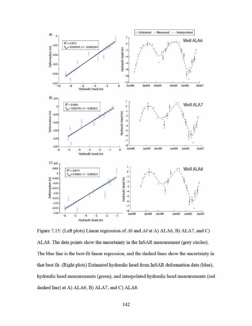
143

Well ALA8 is also located in the subsidence bowl area as seen in the raw interferograms,

but approximately 2 km northwest of the ALA6/ALA7 wells. The regression of Δh and

Δd in Figure 7.15C shows a linear relationship at well ALA8 (R2 = 0.814). The slope of

the regression line is Ske = 6.50 ×10-3 +/- 5.3 ×10-4, and we see that the estimated

hydraulic head agrees with the measured hydraulic head 40% of the time (right plot

7.15C). We can see that the agreement between the estimated hydraulic head and the

interpolated hydraulic head is worse during time periods with few hydraulic head

measurements (see January 2000 – January 2001).

The results of the regression analysis for all 11 wells are shown in Table 7.1. In the work

to follow we discuess how the quality of the linear relationship between the hydraulic

head and the deformation varies based on magnitude of Δh, Sske and b* (see equation

2.26). If these variables are small at the well in question we do not expect the

deformation to be large enough to be accurately measured by InSAR (see discussion in

section 4.2).

Table 7.1 shows the aggregate variable, seasonal hydraulic head change (

�

Δhs), which is

the average seasonal peak-to-trough change in hydraulic head (used previously in section

4.2). The three wells at the top of Table 7.1 (ALA6, ALA7 and ALA8) show large

seasonal hydraulic head change and the regression analysis suggested a linear relationship

between the deformation and the hydraulic head, as predicted in section 4.2. However,

contrary to our predictions in section 4.2 the 8 other pairs of hydraulic head and

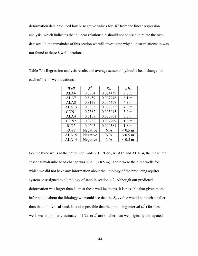
144

deformation data produced low or negative values for from the linear regression

analysis, which indicates that a linear relationship should not be used to relate the two

datasets. In the remainder of this section we will investigate why a linear relationship was

not found at these 8 well locations.

Table 7.1: Regression analysis results and average seasonal hydraulic head change for

each of the 11 well locations.

Well R2 Ske Δhs ALA6 0.8754 0.004439 7.6 m ALA7 0.8459 0.007946 6.1 m ALA8 0.8137 0.006497 4.3 m ALA13 0.0865 0.000655 4.3 m CON1 0.2382 0.003045 3.0 m ALA4 0.0157 0.000961 3.0 m CON2 0.0732 0.002299 1.8 m RIO2 0.0205 0.000381 1.8 m RG88 Negative N/A < 0.5 m

ALA15 Negative N/A < 0.5 m ALA14 Negative N/A < 0.5 m

For the three wells at the bottom of Table 7.1, RG88, ALA15 and ALA14, the measured

seasonal hydraulic head change was small (< 0.5 m). These were the three wells for

which we did not have any information about the lithology of the producing aquifer

system so assigned to a lithology of sand in section 4.2. Although our predicted

deformation was larger than 1 cm at these well locations, it is possible that given more

information about the lithology we would see that the Sske value would be much smaller

than that of a typical sand. It is also possible that the producing interval (b*) for these

wells was improperly estimated. If Sske or b* are smaller than we originally anticipated

€

R2

145

then it is possible that the amount of deformation occurring at these well locations is too

small to be accurately measured by InSAR.

There remain five wells, ALA13, CON1, ALA4, CON2 and RIO2, where Δhs is large

enough to result in accurate measurements of Δd, but a linear relationship is not observed

between the deformation and the hydraulic head. At these five well locations Sske and b*

may be smaller than we estimated in section 4.2. This result would affect the amount of

deformation that occurred at the surface and the quality of the linear relationship between

Δh and Δd.

Driller’s logs and geophysical logs from wells CON2, ALA4 and CON1 show that these

wells may be producing water from hard rock sediments, which have very low values for

Sske. The lower bound predictions of the deformation at these three well locations were

below the sensitivity of the InSAR measurement (see section 4.2). The driller’s log for

well CON2 show that it is producing water from a zone of fractured volcanics, which

generally have

�

Sske of zero. The driller’s log for well ALA4 shows that the main

production layers contain mainly hard rock materials, or hard packed sand/gravel at

depths of over 1000 ft, also exhibiting low

�

Sske values. The driller’s log for well CON1

also shows volcanics with low

�

Sske values. However, the geophysical logs identify the

producing zones of the aquifer and do not indicate that the well was actually producing

from the volcanic layers. Therefore, it is possible that at these three well locations the

deformation is not large enough to be accurately measured by InSAR.

146

The final two wells for discussion in Table 7.1 are ALA13 and RIO2. Both wells are very

deep, 1784 ft and 1396 ft respectively. ALA13 is located in the Closed Basin section of

the SLV. In the Closed Basin water is being pumped from the unconfined aquifer into the

Rio Grande River to meet the demands of the Rio Grande Compact. It was likely drilled

deep in order to avoid the over 900 ft of blue clay sediments recorded in the driller’s log.

Even at the producing depth there are many thick intervals of what is known as “tan clay”

in the SLV. For this reason we hypothesize that the relationship between deformation and

hydraulic head at ALA13 is non–linear, i.e. the deformation may be experiencing a time

lag in relation to the hydraulic head change (equation 2.18). The hydraulic head data were

only recorded from 1999 – 2012, which coincides with only seven SAR acquisition times

over the span of the 1999 – 2000 year. Therefore, a rigorous analysis of the time lag

associated with the elastic deformation of the clays is not likely to produce useful results,

and we did not attempt it.

The driller’s log for well RIO2 does not show the same thick sequence of clay units, as it

is located in the western part of the SLV near the Rio Grande River. However, it is

possible that the estimates of Sske and b* that we provided in section 4.2 were too large. It

is also true that the lower bound of the predicted deformation from section 4.2 was below

the accuracy of the InSAR deformation measurement.

It is important to note that we have not discussed atmospheric phase effects as a factor

that may affect the relationship between Δh and Δd at some of the well locations. Because

our version of SBAS analysis does not include atmospheric temporal filtering (introduced

147

in Section 2.1.2), there will likely be a significant, unaccounted for, amount of

atmospheric phase in each deformation time-series. However, given the results observed

at wells ALA6, ALA7 and ALA8, it appears that given large changes in hydraulic head,

and favorable hydrogeologic conditions (the magnitude of Sske and b*) the InSAR data

and hydraulic head data can exhibit a reliable linear relationship.

7.4.3 Predicting hydraulic head at wells ALA6, ALA7 and ALA8

We used the linear fit between the hydraulic head data and kriged deformation

data to predict hydraulic head at three of the well locations, ALA6, ALA7 and ALA8, for

the entire InSAR data time span (1992 – 2000). Once again, we assumed elastic

compaction, so that the slope of the regression line is an estimate of the elastic skeletal

storage coefficient (Ske) (equation 2.26). Figure 7.16 shows the predicted hydraulic head

at the three well locations.

At each of the three well locations we can see that a seasonal trend in the predicted

hydraulic head values does exist back to 1992. In the winter of 1996 we can see that the

hydraulic head was predicted to be particularly high at all three wells. It is possible that

the phase measured at the January 1996 acquisition time contains uncertainty due to

atmospheric phase effects. Although no precipitation data were available through the

RGDSS, we did investigate three well locations where hydraulic head was collected

during 1996. At wells, SAG7, CON1 and ALA2 the measured hydraulic heads exhibited

a larger high in 1996 than in 1992 – 1995 and 1997 – 2000.

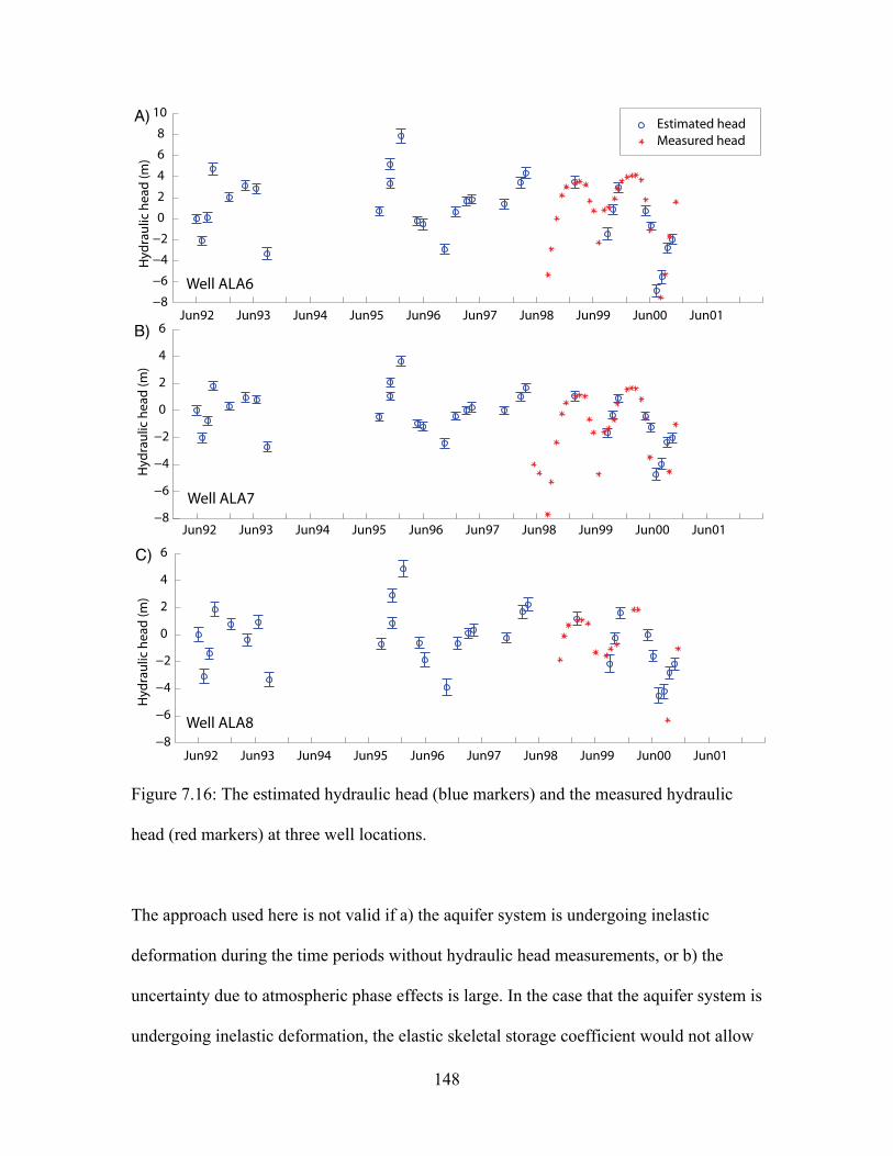
148

Figure 7.16: The estimated hydraulic head (blue markers) and the measured hydraulic

head (red markers) at three well locations.

The approach used here is not valid if a) the aquifer system is undergoing inelastic

deformation during the time periods without hydraulic head measurements, or b) the

uncertainty due to atmospheric phase effects is large. In the case that the aquifer system is

undergoing inelastic deformation, the elastic skeletal storage coefficient would not allow

!8!6!4!202468

10

Hyd

raul

ic h

ead

(m)

Estimated headMeasured head

Jun92 Jun93 Jun94 Jun95 Jun96 Jun97 Jun98 Jun99 Jun00 Jun01!8

!6

!4

!2

0

2

4

6

!8

!6

!4

!2

0

2

4

6

Well ALA6

Well ALA7

Well ALA8

A)

B)

C)

Hyd

raul

ic h

ead

(m)

Hyd

raul

ic h

ead

(m)



149

for the prediction of hydraulic head back in time, and more hydraulic head data would be

needed in order to understand the inelastic relationship. Also, if the unused InSAR

deformation data in the regression analysis (from 1992 – 1998 in the SLV dataset)

contain significant uncertainty due to atmospheric phase effects, the estimates of the

hydraulic head would also be incorrect. However, as discussed in the previous paragraph,

if nearby hydraulic head data are available it is possible to use those data to differentiate

outliers due to atmospheric phase effects from periods with large changes in hydraulic

head.

Although a spatially exhaustive valley wide comparison was not possible, the estimated

hydraulic head at these three well locations provides information about the hydrologic

system through time. The InSAR data have enabled us to look back through the 1990s, an

important time for the management of the confined aquifer system in the SLV, and

determine that the hydraulic head did not exhibit a negative linear trend at these locations

from 1992 - 2000. This has implications for improving the estimation of hydraulic head at

wells in other areas, agricultural or otherwise, with incomplete or sparsely sampled

hydraulic head time series.

7.5 Conclusions

In this chapter we investigated how the relationship between InSAR deformation

measurements and hydraulic head measurements can be used to interpolate and

extrapolate the hydraulic head measurements in the San Luis Valley, Colorado through

time. Initially we focused on the relationship between the hydraulic head measurements

150

and the deformation measurements around a given well location. In order to better

understand how the relationship varied around a well we also investigated the spatial

structure of the two datasets. Based on this analysis we were able to apply simple kriging

to the deformation data, investigate the relationship directly at 15 well locations, and

predict the hydraulic head change during a time when no hydraulic head data were

measured at 3 well locations.

The spatial variability in the hydraulic head dataset was discussed in section 7.3.3. The

variogram analysis showed that with only 11 hydraulic head measurements over 10,000

km2, there was no identifiable spatial structure for the SLV hydraulic head dataset. In

order for this type of research to be applied on a valley wide scale, it is critical that the

hydraulic head dataset exhibit some spatial structure, i.e. the variogram analysis should

show that the hydraulic head measurements made at the wells are spatially related.

We investigated the spatial structure of the InSAR deformation dataset in section 7.3.2. In

Chapter 5, for the purposes of a preliminary analysis, we assumed that the deformation

did not vary on scales < 1 km around three well locations. However, the variogram

analysis in this chapter showed that on average the deformation does vary on scales < 1

km. The spatial structure of the deformation was also found to vary with time. The type

of deformation we are trying to measure, i.e. rapid seasonally variable deformation due to

groundwater pumping and recharge, makes it difficult to process the data and remove

uncertainty due to atmospheric phase effects. Hence, it is difficult to determine which

component of the spatial structure is due to deformation and which component is due to

151

atmospheric phase effects. If the data are sampled more regularly, on the order of two or

three times per month, a processing technique could be developed to differentiate the

seasonal deformation signal from the signal due to atmospheric phase effects.

The results of the deformation spatial analysis allowed for the kriging of the deformation

data at the well locations. The kriged deformation estimates were then compared with

hydraulic head measurements at 11 well locations, and showed a linear relationship at the

three wells with the highest seasonal hydraulic head change (ALA6, ALA7 and ALA8).

Wells with low seasonal changes in hydraulic head, low rock compressibility conditions

or high clay content, did not exhibit a linear relationship between the InSAR deformation

data and the hydraulic head data (as predicted by equations 2.18 and 2.26). These factors

affect the amount of deformation at the surface that can be accurately measured using

InSAR. Given that the two datasets do not agree at a majority of the well locations, it

would be difficult to conduct a valley wide analysis of the deformation and hydraulic

head in the SLV. However, in other aquifer systems that contain more compressible

sediments and/or exhibit larger changes in hydraulic head, a regional-scale analysis might

be possible.

At specific well locations the deformation data were used to fill in the temporal gaps in

the hydraulic head dataset, see section 7.4.3. For wells ALA6, ALA7 and ALA8 this

analysis showed that for the period 1992 – 2000 the hydraulic head did not decrease

linearly with time. These results are especially important for the management of

groundwater in the SLV, where the Confined Aquifer Rules decision requires that

152

hydraulic head levels remain above those measured from 1970 – 2000. Similarly, in other

agricultural areas where irrigation uses groundwater from confined aquifers, the use of

InSAR data at specific well locations may be able to provide information needed for

better management.

153

Chapter 8

Conclusions

8.1 Summary of research

The overall goal of this thesis was to determine to what extent InSAR deformation

data could be used to improve estimates of hydraulic head in the San Luis Valley,

Colorado. The studies in Chapters 5 and 6, where we determined the quality and

uncertainty in the InSAR deformation measurements, positioned us to answer this

question in Chapter 7. Below is a restatement of the contributions of this thesis:

• Modification of a time-series processing algorithm to properly estimate deformation

signals produced by seasonal pumping and recharge of groundwater aquifers in

agricultural areas.

• Development of an extensive time-series of InSAR deformation maps for the San

Luis Valley, Colorado, visualizing the spatial and temporal characteristics of land

154

surface deformation in this region.

• Verification that high quality InSAR deformation measurements can be made in

agricultural areas like the San Luis Valley.

• Estimatation of the uncertainty in the InSAR deformation measurements and

propagated this uncertainty through the data processing chain.

• Adaptation of a time-series processing algorithm such that high quality data are

selected based upon the uncertainty of the final deformation time-series.

• Investigation of the spatial structure of the InSAR measured deformation dataset

and the hydraulic head dataset in the SLV.

• Prediction of hydraulic head back in time at three well locations in the SLV.

In Chapter 5 we determined that the InSAR deformation data in the SLV was of high

quality. We altered the standard SBAS processing algorithm to accommodate short-term

seasonal changes in the deformation due to groundwater pumping and recharge. In

altering the SBAS analysis algorithm we found that our data were more predisposed to

contain atmospheric phase effects, which could add uncertainty into the InSAR

deformation measurement. We determined that many of the small areas, left unwatered

by the center-pivot irrigation systems, yield high quality InSAR data when processed

using SBAS analysis. The InSAR deformation measurements showed the same seasonal

periodicity as the hydraulic head data from monitoring wells. When hydraulic head was

estimated from the InSAR data (with error bars on the order of meters), we found good

agreement with the measured head values. However, we acknowledged that the errors are

so large that these hydraulic head estimates would not provide the level of accuracy

155

required by the RGDSS. Hence, the next component of our research was to focus on the

uncertainty in the InSAR deformation measurement.

In Chapter 6 we quantified the uncertainty in the InSAR deformation measurement due to

decorrelation of radar signals. We found that the uncertainty due to decorrelation was

small when compared to the uncertainty due to atmospheric phase effects. That being the

case, we also investigated the efficacy of an algorithm that uses hydrologic data to

identify scenes whose phase measurements may have been corrupted with atmospheric

phase effects. Although the algorithm worked well with a synthetic dataset, we did not

have a supplementary deformation dataset to validate the algorithm in the SLV. Finally,

we investigated how we can achieve a set level of uncertainty in our InSAR deformation

measurements by predetermining appropriate coherence thresholds for SBAS analysis.

We quantified the relationship between the mean coherence, the standard deviation of the

coherence and the standard deviation of the estimated deformation. These results will

allow researchers to estimate the uncertainty of a dataset before performing all of the

SBAS analysis processing steps. Quantifying the uncertainty in the InSAR measured

deformation is critical if these data are to be used for groundwater applications as a basis

for management decisions.

Groundwater sustainability in the SLV is of utmost importance to groundwater managers,

as is the case in many agricultural areas. The managers in the SLV want to know: a) if

inelastic deformation was occurring in the confined aquifer system, and b) the extent to

which InSAR could be used to satisfy the requirements of the Confined Aquifer Rules

156

Decision. When evaluating the deformation time-series at the 11 wells where we

predicted the highest magnitude of deformation, we concluded that no inelastic

deformation was being detected from 1992 – 2000 (section 5.6). Having satisfied the first

request of the groundwater managers we turned our focus on the problem of using the

InSAR deformation data to improve our understanding of hydraulic head in the confined

aquifer system.

In Chapter 7 we used the relationship between InSAR deformation measurements and

hydraulic head measurements to temporally interpolate and extrapolate hydraulic head in

the confined aquifer system of the San Luis Valley, Colorado. Given that the only

validation for the deformation data was hydraulic head measurements made at wells, we

began by attempting to understand how the relationship varied around three different

wells. We found that the deformation was varying on a scale less than 1 km around the

well locations. We proceeded to investigate the spatial structure of both the deformation

and hydraulic head datasets. The deformation dataset exhibited spatial structures that

could be captured by analytical semi-variogram models. However, the hydraulic head

dataset was too sparsely sampled spatially to draw any conclusions about spatial

structure. We were then able to apply simple kriging to the deformation data using the

semi-variogram models previously calculated. The relationship between hydraulic head

and deformation was explored directly at 11 well locations. Based on these results and the

known uncertainty of the InSAR deformation measurements we investigated the

conditions under which we were able to observe a linear relationship between InSAR

measured deformation and hydraulic head. Given that the two datasets did not show a

157

linear relationship at a majority of the well locations, it was impossible to perform a

valley wide analysis of the deformation and hydraulic head in the SLV. However, in

other aquifer systems that contain more compressible sediments and/or exhibit larger

changes in hydraulic head, a regional-scale analysis would be possible.

At three specific well locations, ALA6, ALA7 and ALA8, we were able to achieve the

overall goal for this thesis. The InSAR measured deformation data were used to fill in

temporal gaps in the hydraulic head dataset. We see InSAR data as providing a new way

to complement expensive and spatially sparse groundwater monitoring wells with a more

economical method of collecting field data. The incorporation of InSAR data could be an

affordable way to centralize systems for the monitoring of groundwater aquifers.

8.2 Opportunities for future research

Although a number of researchers have investigated groundwater problems using

InSAR deformation data, there are still many avenues for future research.

At the most basic level it is important that research continues in agricultural areas.

Although the data are of lower quality than in urban/arid areas, groundwater management

in these areas is of utmost importance. A number of satellites are now collecting SAR

data at longer wavelengths, which is more ideal for vegetated areas. In this thesis we have

shown that by altering processing techniques and using subsidiary data we can process

even the shorter wavelength data and achieve accurate results.

158

There still exist many components of the SBAS analysis algorithm that could be

improved to facilitate the use of InSAR data for groundwater applications. In agricultural

areas where the amplitude of the seasonal signal changes from year to year,

differentiating seasonal signals from phase change due to atmospheric phase effects

becomes difficult. However, as mentioned briefly in Chapter 6 it may be possible to use

pumping data, i.e. extraction rates or volume of water extracted, as prior information

when applying the low-pass deformation model. The pumping data could be used to

determine when the onset of seasonal subsidence should occur each year. Using pumping

data would also be advantageous because it is often more readily available to

groundwater managers than hydraulic head data.

Although we were able to predict hydraulic head at a number of locations in the SLV, the

overall goal of this research was to be able to do so for the entire SLV. We believe that

future research should focus on data driven applications rather than working with large

over parameterized groundwater flow models. It is possible that given the right dataset,

where the deformation was large enough and you had enough hydraulic head

measurements for calibration, that a large-scale analysis could be performed. A number

of stochastic techniques employ a data driven approach, e.g. Bayesian Maximum Entropy

and Artificial Neural Networks, and could be used to interpolate between the hydraulic

head measurements made in wells. These techniques would work well whether elastic or

inelastic deformation was taking place.

159

The spatial analysis of the InSAR deformation data and hydraulic head data was a

component of the thesis that could be improved upon given more spatially dense

hydraulic head measurements. Alternatively, some simple synthetic studies investigating

the semi-variogram models for phase change due to atmospheric phase effects and

deformation due to hydraulic head change would be very useful during the

implementation of the stochastic methods described above. Characterizing correlation

lengths for specific areas of aquifer systems may even be able to differentiate spatial

changes in hydrogeologic facies. This too could be investigated through a number of

simple synthetic examples.

This thesis focused directly on the link between deformation and hydraulic head in order

to satisfy the requirements of the Confined Aquifer Rules Decision. However, as was

discovered during the process of evaluating the hydraulic head data, the quantity of data

available was quite small. In the SLV and in many other agricultural areas with

groundwater management issues, local and state governments have begun to regulate

groundwater withdrawals. Because of these regulations monitoring devices have been

placed on wells in order to determine the extraction rates. If we know that the main cause

for the hydraulic head change seasonally is due to the extraction of water then it might be

possible to avoid the middle parameter (hydraulic head change) and calibrate directly to

the forcing function (the pumping of the well). If it could be shown that this type of

calculation is simpler and legally easier to regulate then it is possible that groundwater

management policy could change. Instead of the Confined Aquifer Rules decision

160

requiring that the hydraulic head remain between levels measured from 1970 – 2000, it

could describe some sustainable extraction rate for each well.

As recently done in California with the passage of Senate Bill 6, it is likely that

legislation will be put in place in many western states with requirements to monitor and

report hydraulic head or extraction rates. With further development, we are optimistic

that InSAR could provide the measurements to cost effectively meet the needs of such

legislation, thus facilitating the implementation and adoption of the legislation. If we are

to use monitoring of groundwater aquifers to effectively meet the global challenge of

managing our water resources, we need robust, reliable, cost-effective forms of

monitoring. We believe that InSAR and other satellite-based methods of data acquisition

have great potential to address this need, thus leading to improved methods of

groundwater management.

161

References

Agram, P. S. (2010), Persistent scatterer interferometry in natural terrain, Stanford

University.

Amelung, F., D. L. Galloway, J. W. Bell, H. A. Zebker, and R. J. Laczniak (1999),

Sensing the ups and downs of Las Vegas: InSAR reveals structural control of land

subsidence and aquifer-system deformation, Geo, 27(6), 483-486.

Anderssohn, J., H. U. Wetzel, T. R. Walter, M. Motagh, Y. Djamour, and H. Kaufmann

(2008), Land subsidence pattern controlled by old alpine basement faults in the

Kashmar Valley, northeast Iran: results from InSAR and levelling, GeoJI, 174(1),

287-294.

Anderssohn, J., M. Motagh, T. R. Walter, M. Rosenau, H. Kaufmann, and O. Oncken

(2009), Surface deformation time series and source modeling for a volcanic

complex system based on satellite wide swath and image mode interferometry:

The Lazufre system, central Andes, RSEnv, 113, 2062-2075, DOI:

10.1016/j.rse.2009.05.004.

162

Barber, B. C. (1993), The phase statistics of a multichannel radar interferometer, Waves

in Random Media, 3(4), 257-266.

Batu, V. (1998). Aquifer hydraulics: a comprehensive guide to hydrogeologic data

analysis. Wiley-Interscience.

Bawden, G. W., W. Thatcher, R. S. Stein, K. W. Hudnut, and G. Peltzer (2001), Tectonic

contraction across Los Angeles after removal of groundwater pumping effects,

Natur, 412(6849), 812-815.

Bell, J. W., F. Amelung, A. Ferretti, M. Bianchi, and F. Novali (2008), Permanent

scatterer InSAR reveals seasonal and long-term aquifer-system response to

groundwater pumping and artificial recharge, WRR, 44(W02407), DOI:

10.1029/2007WR006152.

Berardino, P., G. Fornaro, R. Lanari, and E. Sansosti (2002), A New Algorithm for

Surface Deformation Monitoring Based on Small Baseline Differential SAR

Interferograms, ITGRS, 40(11), 2375-2383.

Biot, M. A. (1941), General theory of three-dimensional consolidation, JAP, 12, 155-164.

Canuti, P., N. Casagli, P. Farina, A. Ferretti, F. Marks, and G. Menduni (2006), Analysis

of subsidence phenomena in the Arno river basin using radar interferometry,

Giornale di Geologia Applicata 4, 131-136.

Calderhead, A. I., R. Therrien, A. Rivera, R. Martel, J. Garfias (2011), Simulating

pumping-induced regional land subsidence with the use of InSAR and field data

in the Toluca Valley, Mexico, Advances in Water Resources, 34, 83-97.

163

Carslaw, H. S., and J. C. Jaeger (1959), Conduction of heat in solids. , edited, Oxford at

the Clarendon Press, London.

Chatterjee, R., B. Fruneau, J. Rudant, P. Roy, P. L. Frison, R. Lakhera, V. Dadhwal, and

R. Saha (2006), Subsidence of Kolkata (Calcutta) City, India during the 1990s as

observed from space by differential synthetic aperture radar interferometry (D-

InSAR) technique, RSEnv, 102(1), 176-185.

Chen, C. W., and H. Zebker (2002), Phase Unwrapping for Large SAR Interferograms:

Statistical Segmentation and Generalized Network Models, ITGRS, 40(8), 1709-

1719.

Deutsch, C. V., & Journel, A. G. (1992). Geostatistical software library and user&s

guide (Vol. 1996). New York: Oxford university press.

Emery, P. A., R. J. Snipes, J. M. Dumeyer, and J. M. Klein (1973), Water in the San Luis

Valley, south-central Colorado, Colorado Water Resources Circular, 18, 27.

Fattahi, H., and F. Amelung (2013), DEM Error Correction in InSAR Time Series,

Geoscience and Remote Sensing, IEEE Transactions on, PP(99), 1-11, DOI:

10.1109/tgrs.2012.2227761.

Ferretti, A., C. Prati, and F. Rocca (2000), Nonlinear subsidence rate estimation using

permanent scatterers in differential SAR interferometry, ITGRS, 38(5), 2202-

2212.

Ferretti, A., C. Prati, and F. Rocca (2001), Permanent Scatterers in SAR Interferometry,

ITGRS, 39(1), 8-20.

164

Fetter, C. W. (2001), Applied Hydrogeology. , edited, Prentice-Hall Inc., Upper Saddle

River, New Jersey.

Galloway, D. L., K. W. Hudnut, S. E. Ingebritsen, S. P. Phillips, and G. Peltzer (1998),

Detection of aquifer system compaction and land subsidence using interferometric

synthetic aperture radar, Antelope Valley, Mojave Desert, California, WRR,

34(10), 2573-2585.

Gonzalez, P., J., and J. Fernandez (2011), Error estimation in multitemporal InSAR

deformation time series, with application to Lanzarote, Canary Islands, JGR,

116(B10404), DOI: 10.1029/2011JB008412.

Goodman, N. R. (1963), Statistical Analysis Based on a Certain Multivariate Complex

Gaussian Distribution (An Introduction), The Annals of Mathematical Statistics,

34(1), 152-177.

Guarnieri, A. M., and S. Tebaldini (2007), Hybrid Cramer-Rao Bounds for Crustal

Displacement Field Estimators in SAR Interferometry, Signal Processing Letters,

IEEE, 14(12), 1012-1015, DOI: 10.1109/lsp.2007.904705.

Hanssen, R. F. (1998), Assessment of the role of atmospheric heterogeneities in ERS

tandem SAR interferometry, Delft University, Delft, Netherlands.

Hanssen, R. F. (2001), Radar Interferometry – Data Interpretation and Error Analysis,

Kluwer Academic Publishers.

Harmon, E. (2001), RGDSS Ground Water, Task 28 – Confined Aquifer Testing

Piezometer no. 5, Three S Ranch well 15926R, HRS Water Consultants Inc.

165

Hearne, G. A., and J. D. Dewey (1988), Hydrologic analysis of the Rio Grande Basin

north of Embudo, New Mexico, Colorado and New Mexico, U.S. Geological

Survey Water-Resources Investigations Report, 86–4113, 244.

Hoen, W. (2001), A Correlation-based Approach to Modeling Interferometric Radar

Observations of the Greenland Ice Sheet, Stanford University, Stanford.

Hoffmann, J., H. Zebker, D. Galloway, and F. Amelung (2001), Seasonal subsidence and

rebound in Las Vegas Valley, Nevada, observed by synthetic aperture radar

interferometry, WRR, 37(6), 1551-1566.

Hoffmann, J. (2003), The Application of Satellite Radar Interferometry to the Study of

Land Subsidence over Developed Aquifer Systems, 229 pp, Stanford University,

Stanford.

Hoffmann, J., D. L. Galloway, and H. A. Zebker (2003), Inverse modeling of interbed

storage parameters using land subsidence observations, Antelope Valley,

California, WRR, 39(2), 1031-1043, DOI: 10.1029/2001WR001252.

Hooper, A., H. Zebker, P. Segall, and B. Kampes (2004), A new method for measuring

deformation on volcanoes and other natural terrains using InSAR persistent

scatterers, GeoRL, 31(L23611), DOI: 10.1029/2004GL021737.

HRS Water Consultants Inc., (2002), Task 32 Hydrogeologic Database Refresh Final

Memorandum, Map 35. For Rio Grande Decision Support System, Colorado

Water Conservation Board and Colorado Division of Water Resources.

166

Hung, W. C., C. Hwang, C. P. Chang, J. Y. Yen, C. H. Liu, and W. H. Yang (2010),

Monitoring severe aquifer-system compaction and land subsidence in Taiwan

using multiple sensors: Yunlin, the southern Choushui River Alluvial Fan,

Environmental Earth Sciences, 59(7), 1535-1548.

Ireland, R. L., J. F. Poland, and F. S. Riley (1984), Land subsidence in the San Joaquin

Valley, California, as of 1980, U.S. Geological Survey Professional Paper, 437-I,

93, 1984.

Jorgensen, D. G. (1980), Relationships between basic soils – engineering equations and

basic ground-water flow equations, Water-Supply Paper U.S. Geological Survey,

2064.

Kitanidis, P. K. (1997). Introduction to geostatistics: applications in hydrogeology.

Cambridge University Press.

Knospe, S., and S. Jonsson (2010), Covariance Estimation for dInSAR Surface

Deformation Measurements in the Presence of Anisotropic Atmospheric Noise,

IEE Transactions on Geoscience and Remote Sensing, 48(4), DOI:

10.1109/TGRS.2009.2033937.

Kuenhold, O. J. (2006), Confined Aquifer New Use Rules for Division 3: Findings of

Fact, Conclusions of Law, Judgement and Decree, edited, District Court, Water

Division No. 3, Colorado.

167

Kwoun, O.-l., L. Zhong, C. Neal, and C. Wicks (2006), Quiescent deformation of the

Aniakchak Caldera, Alaska, mapped by InSAR, Geo, 34(1), 5-8, DOI:

10.1130/G22015.1.

Larsen, Y., G. Engen, T. R. Lauknes, E. Malnes, and K. A. Hogda (2005), A generic

differential InSAR processing system, with applications to land subsidence and

SWE retrieval, paper presented at Advances in SAR Interferometry from

ENVISAT and ERS missions (Fringe 2005), ESA ESRIN, Frascati, Italy,

November 28 - December 2, 2005.

Lauknes, T. R. (2004), Long-Term Surface Deformation Mapping using Small-Baseline

Differential SAR Interferograms, 100 pp, University of Tromso, Tromso.

Lauknes, T. R., J. Dehls, A. Hogda, Y. Larsen, and D. J. Weydahl (2005), A comparison

of SBAS and PS ERS InSAR for subsidence monitoring in Oslo, Norway, In

Proc. FRINGE-2005 Workshop, Frascati, 28 Nov–2 Dec.

Leake, S. A., and D. E. Prudic (1991), Documentation of a computer program to simulate

aquifer-system compaction using the modular finite-difference ground-water flow

model, USGS Techniques of Water-Resources Investigations, 6(A2), 68.

Lee, J., A. R. Miller, and K. W. Hoppel (1994), Statistics of phase difference and product

magnitude of multi-look processed Gaussian signals, Waves in Random Media,

4(3), 307-319.

Massonnet, D., and K. L. Feigl (1998), Radar interferometry and its application to

changes in the Earth’s surface, RvGeo, 36(4), 441-500.

168

Meyer, B., R. Armijo, D. Massonnet, J. B. d. Chabalier, C. Delacourt, J. C. Ruegg, J.

Achache, P. Briole, and D. Papanastassiou (1996), The 1995 Grevena (Northern

Greece) Earthquake: Fault model constrained with tectonic observations and SAR

interferometry, GeoRL, 23(19), 2677-2680.

Onn, F., and H. Zebker (2006), Correction for interferometric synthetic aperture radar

atmospheric phase artifacts using time series of zenith wet delay observations

from a GPS network, JGR, 111(B09102), 16, DOI: 10.1029/2005JB004012

Poland, J. F., B. E. Lofgren, R. L. Ireland, and R. G. Pugh (1975), Land Subsidence in the

San Joaquin Valley, California, as of 1972, U.S. Geological Survey Professional

Paper 437-H, 78.

Reeves, J. A., R. J. Knight, H. Zebker, W. A. Schreüder, P. S. Agram, and T. R. Lauknes

(2011), High quality InSAR data linked to seasonal change in hydraulic head for

an agricultural area in the San Luis Valley, Colorado, WRR, 47, DOI:

10.1029/2010WR010312.

Reeves, J.A., R. Knight, H.A. Zebker, (in revision for IEEE Geoscience and Remote

Sensing), An analysis of the uncertainty in InSAR deformation measurements for

groundwater applications.

RGDSS (2005), Rio Grande Decision Support System Groundwater Model as of July 29,

2005, Principia Mathematica, Lakewood, Colorado.

Riley, F. S. (1969), Analysis of borehole extensometer data from central California,

International Association of Scientific Hydrology Publication, 89, 423-431.

169

Riley, F. S. (1998), Mechanics of aquifer systems – The scientific legacy of Dr. Joseph F.

Poland, in Borchers, J.W., ed., Land subsidence case studies and surrent research:

Proceedings of the Dr. Joseph F. Poland Symposium on Land Subsidence,

Association of Engineering Geologists Special Publication, 8(13-27).

Rocca, F. (2007), Modeling Interferogram Stacks, Geoscience and Remote Sensing, IEEE

Transactions on, 45(10), 3289-3299, DOI: 10.1109/tgrs.2007.902286.

Schmidt, D. A., and R. Burgmann (2003), Time-dependent land uplift and subsidence in

the Santa Clara valley, California, from a large interferometric synthetic aperture

radar data set, JGR, 108(B9), 2416-2428, DOI: 10.1029/2002JB002267.

Scott, R. F. (1963), Principles of soil mechanics, IV: Settlement and consolidation od

clay, Engineering News-Record, 95(22), 874-878.

Simons, M., Y. Fialko, and L. Rivera (2002), Coseismic Deformation from the 1999 Mw

7.1 Hector Mine, California, Earthquake as Inferred from InSAR and GPS

Observations, Bulletin of the Seismological Society of America, 92(4), 1390-1402.

Sneed, M., J. T. Brandt, and C. V. W. District (2007), Detection and Measurement of

Land Subsidence Using Global Positioning System Surveying and Interferometric

Synthetic Aperture Radar, Coachella Valley, California, 1996-2005, US

Department of the Interior, US Geological Survey.

Terzaghi, K. (1925), Structure and volume of voids in soils, translated from

Erdbaummechanik auf Bodenphysikalischer Grundlage, in From Theory to

Practice in Soil Mechanics, John Wiley and Sons, New York.

170

Todd, D. K. (1980), Groundwater Hydrology, 2nd ed., John Wiley, New York.

Tough, R. J. A., D. Blacknell, and S. Quegan (1995), A Statistical Description of

Polarimetric and Interferometric Synthetic Aperture Radar Data, Mathematical

and Physical Sciences, 449(1937), 567-589.

Treuhaft, R. N., & Lanyi, G. E. (1987). The effect of the dynamic wet troposphere on

radio interferometric measurements. Radio Science, 22(2), 251-265.

Usai, S. (2003), A Least Squares Database Approach for SAR Interferometric Data,

ITGRS, 41(4), 753-760, DOI: 10.1109/TGRS.2003.810675.

Watson, K. M., Y. Bock, and D. T. Sandwell (2002), Satellite interferometric

observations of displacements associated with seasonal groundwater in the Los

Angeles basin, JGR, 107(B4), DOI: 10.1029/2001JB000470.

Wiley, B. A., and D. A. Schmidt (2010), Deciphering vertical deformation and

poroelastic parameters in a tectonically active fault-bound aquifer using InSAR

and well level data, San Bernardino basin, California, GeoJI, 181, 1185 - 1200,

DOI: 10.1111/j.1365-246X.2010.04568.x

Wisely, B. A., and D. A. Schmidt (2010), Deciphering vertical deformation and

poroelastic parameters in a tectonically active fault-bound aquifer using InSAR

and well level data, San Bernardino basin, California, GeoJI, 181, 1185 - 1200,

DOI: 10.1111/j.1365-246X.2010.04568.x

Zebker, H., and J. Villasenor (1992), Decorrelation in interferometric radar echoes,

ITGRS, 30(5), 950-959.

171

York, D., Evensen, N. M., Martínez, M. L., & Delgado, J. D. B. (2004). Unified

equations for the slope, intercept, and standard errors of the best straight

line.American Journal of Physics, 72, 367.

Zebker, H., C. L. Werner, P. A. Rosen, and P. Hensley (1994), Accuracy of topographic

maps derived from ERS-1 interferometric radar, ITGRS, 32(4), 823-836.

Zebker, H., P. A. Rosen, and P. Hensley (1997), Atmospheric effects in interferometric

synthetic aperture radar surface deformation and topographic maps, JGR,

102(B4), 7547-7563.

Documents

USING INTERFEROMETRIC SYNTHETIC APERTURE RADAR DATA … · USING INTERFEROMETRIC SYNTHETIC APERTURE RADAR DATA TO ... Zebker is the best co-advisor a girl could ask for. ... Dan Aukes,