Using context information in structured document retrieval: an approach based on influence diagrams

Information Processing and Management 40 (2004) 829–847

www.elsevier.com/locate/infoproman

Using context information in structured document retrieval:an approach based on influence diagrams q

Luis M. de Campos, Juan M. Fern�andez-Luna *, Juan F. Huete

Departamento de Ciencias de la Computaci�on e Inteligencia Artificial, E.T.S.I. Inform�atica,Universidad de Granada, C.P. 18071, Granada, Spain

Available online 4 June 2004

Abstract

In this paper we present an Information Retrieval System (IRS) which is able to work with structured document

collections. The model is based on the influence diagrams formalism: a generalization of Bayesian Networks that

provides a visual representation of a decision problem. These offer an intuitive way to identify and display the essential

elements of the domain (the structured document components and their usefulness) and also how these are related to

each other. They have also associated quantitative knowledge that measures the strength of the interactions. By means

of this approach, we shall present structured retrieval as a decision-making problem. Two different models have been

designed: SID (Simple Influence Diagram) and CID (Context-based Influence Diagram). The main difference between

these two models is that the latter also takes into account influences provided by the context in which each structural

component is located.

� 2004 Elsevier Ltd. All rights reserved.

Keywords: Bayesian networks; Influence diagrams; Structured documents; Retrieval model; Decision theory

1. Introduction

Documents such as textbooks, scientific articles, technical manuals, etc. have two main characteristics:

on the one hand, the set of terms used to describe their contents, and on the other, a well-defined structure

to organize these contents comprehensibly and improve readability for the user. Since both characteristics

are quite important and must be taken into account when writing a document, it is natural to develop tools

capable of representing these documents properly. New formalisms to manage documents, such as HTML,

XML or MPEG-7, have been designed to tackle this problem, being capable of representing both the

content and the structure of a document.

qThis work has been jointly supported by the Spanish Fondo de Investigaci�on Sanitaria and Consejer�ıa de Salud de la Junta de

Andaluc�ıa, under Projects PI021147 and 177/02, respectively.* Corresponding author.

E-mail addresses: [email protected] (L.M. de Campos), [email protected] (J.M. Fern�andez-Luna), [email protected] (J.F.

Huete).

0306-4573/$ - see front matter � 2004 Elsevier Ltd. All rights reserved.

doi:10.1016/j.ipm.2004.04.014

mail to: [email protected]

830 L.M. de Campos et al. / Information Processing and Management 40 (2004) 829–847

In general, when a document is represented by means of content and also structure, it is called a

structured document, in contrast to the (plain) classical representation of a document. Nowadays, these

formalisms are widely used to manage electronic documents and, as a result, more and more structured

documents have become available. This structural knowledge can be exploited when designing an Infor-mation Retrieval System (IRS) (Chiaramella, 2001) in order to obtain a more intelligent performance and

therefore one which better satisfies the user’s needs. The aim of the system is therefore to retrieve the set of

document components which are most relevant to a query (not necessarily an entire document). In order to

achieve this aim, it is necessary to design and implement models and tools to index, retrieve, and present

documents according to the given structure.

Classical IRSs consider each document as an atomic item of information, which is handled in isolation.

For example, a probabilistic IRS ranks the documents by considering their probability of relevance to a

given query. These values are usually computed without taking into account the rest of the documents inthe collection. Therefore, the action of presenting (or not presenting) a document to the user is independent

of the action of presenting (or not presenting) any other document.

Although this procedure is valid for classical document collections, it cannot be applied properly when

dealing with structured documents. Now, the situation is different: rather than being interested in retrieving a

whole document, we might be interested in retrieving document units or components. Once the relevance

probability of each structural unit has been computed and a ranking with all of these has been generated,

the user can retrieve redundant information. For example, let us suppose that the top of the ranking of

units is composed of the three subsections of a section from the same article, and the fourth item is thesection itself. The system should detect this situation and decide to show either these three subsections or

only the section, but not the four units. In this case, it would probably be better to retrieve only the whole

section. It is clear that the decision to show a document unit affects the retrieval of other units.

One possible solution to these problems is to make a decision about what to retrieve, depending not only

on the probability of relevance of the units but also in terms of the usefulness of these units for the user and

what has been previously retrieved. For instance, if a user is interested in the Runge–Kutta method for

numerical integration of ordinary differential equations, they would not be interested in either a whole book

being retrieved or only the five equations defining the method being returned. What the user would beinterested in, however, would be certain parts of the book where the formulas themselves were accompanied

by additional information so that they could be understood (notation, description of the method, etc.). In

other words, what it is being pursued is to provide an IRS with the capacity to automatically select those

more appropriate units (the best entry points to the relevant documents).

In an attempt to solve these problems, we propose a model which is capable of making decisions, i.e. the

system should be able to determine those units to be retrieved, not only depending on the probability of

relevance, but also on the utility of these units for the user (possibly taking into account the user’s own

preferences). This will be carried out by means of an Influence diagram (Jensen, 2001), a generalization ofthe well founded Bayesian network formalism (Pearl, 1988). Bayesian networks have been successfully

applied for dealing with classical Information Retrieval (IR) (de Campos, Fern�andez-Luna, & Huete,

2003a; Ribeiro-Neto & Muntz, 1996; Turtle & Croft, 1990) and also for structured Information Retrieval

(Crestani, de Campos, Fern�andez-Luna, & Huete, 2003; Graves & Lalmas, 2002; Myaeng, Jang, Kim, &

Zhoo, 1998; Piwowarski, Faure, & Gallinari, 2002). Influence diagrams can show the structure of a decision

problem, since they are an intuitive, effective formalism for representing, understanding and explaining the

decision models, and have a high expressive power.

In this paper, Section 2 introduces basic concepts about influence diagrams and the type of documentsthat we are going to work with. In Section 3, we present the two proposed influence diagram models: SID

(simple influence diagram) and CID (context-based influence diagram). Section 4 shows how an influence

diagram can be solved and how to apply the results obtained after this process to structured IR. The

experimental results will be discussed in Section 5 and finally, Section 6 presents the conclusions of the paper.

L.M. de Campos et al. / Information Processing and Management 40 (2004) 829–847 831

2. Preliminaries

2.1. Influence diagrams

An influence diagram (Jensen, 2001; Shachter, 1988) provides a simple notation for creating decision

models by clarifying the qualitative issues of the factors which need to be considered and how they are

related, i.e. an intuitive representation of the model. They also have associated an underlying quantitative

representation in order to measure the strength of the relationships: we can quantify uncertain interactions

between random variables and also the decision maker’s options and preferences. The model is used to

determine the optimal decision policy.

More formally, an influence diagram is an acyclic directed graph containing three types of nodes

(decision, chance, and value nodes) and two types of arcs (influence and informative arcs).Nodes in an influence diagram represent various types of variables.

• Decision nodes. Usually drawn as rectangles, these represent variables that the decision maker controls

directly. These variables model the decision alternatives available for the decision maker.

• Chance nodes. Usually drawn as circles, these represent random variables, i.e. uncertain quantities that

are relevant to the decision problem and cannot be controlled directly. They are quantified by means of

conditional probability distributions, identical to those used in Bayesian networks. 1 Predecessors (par-

ents) of chance nodes that are decision nodes act in exactly the same way as those predecessors that arechance nodes––they index the conditional probability tables of the child node.

• Utility nodes. Usually drawn as diamonds, these represent utility, i.e. they express the profit or the pref-

erence degree of the consequences derived from the decision process. They are quantified by the utility of

each of the possible combinations of outcomes of their parent nodes.

There are also different types of arcs in an influence diagram, which generally represent influence. The

arcs between chance nodes represent probabilistic dependences (as occurs in Bayesian networks). The arcs

from a decision node to a chance node or to a utility node establish that the future decision will affect thevalue of the chance node or the profit obtained, respectively. Arcs between a chance node and a decision

node (also called informative) only say that the value of the chance node will be known at the moment of

making the decision. Finally, arcs from a chance node to a utility node will represent the fact that the profit

depends on the value that this chance node takes. The absence of an arc between two nodes specifies

(conditional) independence relationships. It should be noted that the absence of an arc is a stronger

statement than the presence of an arc, which only indicates the possibility of dependence.

Some arcs in influence diagrams clearly have a causal meaning. In particular, a directed path from a

decision node to a chance node means that the decision will influence that chance node, in the sense ofchanging its probability distribution.

A simple example of an influence diagram appears in Fig. 1. It has two chance nodes, F and W , rep-

resenting, the weather forecast in the morning (sunny, cloudy or rainy), and whether it actually rains during

the day (rain or no-rain), respectively. It has one decision node U , take an umbrella (with possible values

true or false). The utility node measures the decision maker’s satisfaction.

With each chance node X in the graph, the quantitative part of an influence diagram associates a set of

conditional probability distributions pðX jpaðX ÞÞ, one for each configuration paðX Þ from the parent set of Xin the graph, PaðX Þ, i.e. for each allocation of values to all the variables in the parent set of X . If X has no

1 In fact, the subset of an influence diagram that consists only of chance nodes is a Bayesian network, i.e., an influence diagram can

also be viewed as a Bayesian network enlarged with decision and utility nodes.

Take UmbrellaP(weather = rain) = 0.2

forecast(F)

weather(W)(U)

P(F=sunny|W=rain) =0.1P(F=cloudy|W=rain)=0.4P(F=rainy|W=rain)=0.5P(F=sunny|W=no-rain) =0.7P(F=cloudy|W=no-rain)=0.2P(F=rainy|W=no-rain)=0.1

P(weather = no-rain) = 0.8

Utility(W=no-rain, U=T) =10Utility(W=no-rain, U=F) = 20Utility(W=rain, U=T) = 70Utility(W=rain, U=F) = 0

Utility

Fig. 1. An example of an influence diagram.


parents (PaðX Þ ¼ ;), then pðX jpaðX ÞÞ equals pðX Þ. For each utility node V , a set of utility values vðpaðV ÞÞ is

associated, specifying for each combination of values for the parents of V , a number expressing the

desirability of this combination for the decision maker.The goal of influence diagram modeling is to choose the decision alternative that will lead to the highest

expected gain (utility), i.e. to find the optimal policy (Shachter, 1986; Zhang, 1998). In order to compute the

solution, for each sequence of decisions, the utilities of its uncertain consequences are weighted with the

probabilities that these consequences will occur.

2.2. The document sources

In this section, we introduce the type of structured documents that we shall consider. We start with a

document collection comprising N documents, D ¼ fD1; . . . ;DNg, and the set T ¼ fT1; . . . ; TMg of the Mterms or concepts used to index these documents (the glossary of the collection). AðDiÞ will denote the

subset of terms in T that are used to index the document Di.

We shall assume that each document D is composed of a hierarchical structure of ‘D abstraction levels,L1, L2; . . . ;L‘D , each representing a structural association of elements in the document. For instance,

sections, subsections, and paragraphs in the context of a collection of structured scientific articles, or scenes,

shots, and frames in MPEG-7 videos. Each level contains a set of structural units of a given degree of

specificity (such as Sections 3, 3.2, or paragraph 3.2.15). The level in which the document itself is included

will be denoted by level 1 (L1), and the more specific level by L‘D . In order to simplify the notation, we

assume that the number of levels, ‘D, is the same for all the documents in the collection (‘D ¼ ‘).Each structural unit will be denoted by Ui;j, where i is the identifier of that unit in the level j. The number

of structural units contained in each level Lj is represented by jLjj. Therefore, Lj ¼ fU1;j; . . . ;UjLjj;jg. Theunits are organized according to the current structure of the document: every unit Ui;j at level j, except the

unit at level j ¼ 1 (i.e. the complete document Di ¼ Ui;1), is related to only one unit Uzði;jÞ;j�1 of the lower

level j� 1. 2 As the text (the whole set of terms) associated to Ui;j is part of the text associated to Uzði;jÞ;j�1,

using notation, we shall note this relation as Ui;j Uzði;jÞ;j�1.

Each term Tk 2 AðDiÞ, originally indexing a document Di, will be assigned to those units in level L‘

containing it which are associated with Di. Therefore, only the units in level L‘ will be indexed, having

associated several terms describing their content. Consequently, each structured document may be repre-

sented as a tree (Fig. 2 shows an example).

2 zði; jÞ is a function that returns the index of the unit in level j� 1 to which the unit with index i in level j belongs.

Fig. 2. Structured representation of a document.


3. The influence diagram-based retrieval model for structured documents

An influence diagram consists of a qualitative and a quantitative part. The qualitative part, represented

by a directed acyclic graph, with nodes representing the variables of the decision problem to solve, and arcs

indicating causality, relevance, dependence or influence relationships between the variables. The quanti-

tative component is encoded by means of both conditional probability distributions and utility values. In

order to describe our model, we shall therefore present each of these parts.

3.1. The qualitative component: representing variables and influences

First, the different types of nodes to be used:

• Chance nodes. Our influence diagram will contain two different sets of chance nodes: those associated to

structural units, U ¼ [‘j¼1Lj; and those related to terms, T. Each node represents a binary random var-

iable: Ui;j takes its values in the set fu�i;j; uþi;jg, representing that the unit is not relevant and is relevant,

respectively; 3 Ti takes its values from the set ft�i ; tþi g, where in this case t�i stands for ‘the term Ti is

not relevant’, and tþi represents ‘the term Ti is relevant’. 4 In order to denote a generic, unspecified value

of a term variable Ti or a unit variable Ui;j, we shall use lower-case letters, ti and ui;j. It should be noted

that we employ the notation Ti (Ui;j, respectively) to refer to the term (unit, respectively) and also to its

associated variable and corresponding node.• Decision nodes. These nodes model the decision variables, representing the possible alternatives available

to the decision maker. In our case, we consider one decision node, Ri;j, for each structural unit Ui;j 2 Lj,

8j ¼ 1; . . . ; ‘, 8i ¼ 1; . . . ; jLjj. Ri;j represents the decision variable related to whether or not to show the

content of Ui;j to the user. The two different values for Ri;j are rþi;j and r�i;j, meaning ‘retrieve Ui;j’ and ‘do

not retrieve Ui;j’, respectively.

• Utility nodes. We shall also consider one utility node, Vi;j, for each structural unit Ui;j 2 Lj, 8j ¼ 1; . . . ; ‘,8i ¼ 1; . . . ; jLjj. Vi;j will measure the value of utility of the corresponding decision.

We shall also consider a utility node that represents the joint utility of the whole model. This node will bedenoted by

P, representing the fact that we are assuming an additive behavior of the model.

3 A unit is relevant for a given query if it satisfies the user’s information need expressed by means of this query.4 A term is relevant in the sense that the user believes that this term will appear in relevant documents.


In order to complete the qualitative component, it is necessary to describe the topology of the model, i.e.

the set of arcs used to represent the relationships between the variables described above.

• Arcs pointing to chance nodes. These arcs encode the dependences between the represented statistical vari-ables. The absence of an arc between two nodes means that the corresponding variables do not influence

each other directly and hence are (conditionally) independent.

In our case, we shall consider that there is an arc from a given chance node (either a term or structural

unit) to the particular structural unit node it belongs to. In this case, we are expressing the fact that the

probability of relevance of a given structural unit to the query will depend on the relevance values of the

different elements (units or terms) that comprise it. It should be noted that with this criteria, term nodes

have no parents, i.e. they are root nodes, expressing the fact that they are the most specific items of

information in the model. We do not include arcs from decision nodes to chance nodes, since these arcsexpress an influence on the chance node exerted by the decision maker. In our case, the degree of rel-

evance for a structural unit is independent of the possible decision about whether this unit should be

retrieved or not.

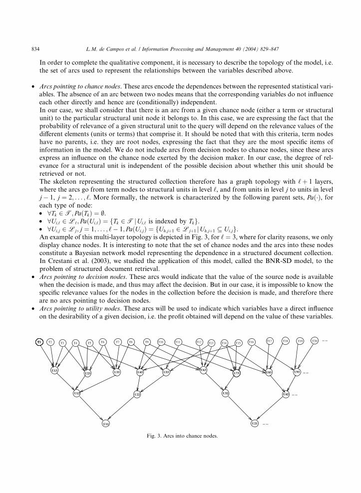
The skeleton representing the structured collection therefore has a graph topology with ‘þ 1 layers,

where the arcs go from term nodes to structural units in level ‘, and from units in level j to units in level

j� 1, j ¼ 2; . . . ; ‘. More formally, the network is characterized by the following parent sets, Pað�Þ, for

each type of node:

• 8Tk 2 T; PaðTkÞ ¼ ;.• 8Ui;‘ 2 L‘; PaðUi;‘Þ ¼ fTk 2 T jUi;‘ is indexed by Tkg.• 8Ui;j 2 Lj; j ¼ 1; . . . ; ‘� 1; PaðUi;jÞ ¼ fUh;jþ1 2 Ljþ1 jUh;jþ1 Ui;jg.An example of this multi-layer topology is depicted in Fig. 3, for ‘ ¼ 3, where for clarity reasons, we only

display chance nodes. It is interesting to note that the set of chance nodes and the arcs into these nodes

constitute a Bayesian network model representing the dependence in a structured document collection.

In Crestani et al. (2003), we studied the application of this model, called the BNR-SD model, to the

problem of structured document retrieval.

• Arcs pointing to decision nodes. These arcs would indicate that the value of the source node is availablewhen the decision is made, and thus may affect the decision. But in our case, it is impossible to know the

specific relevance values for the nodes in the collection before the decision is made, and therefore there

are no arcs pointing to decision nodes.

• Arcs pointing to utility nodes. These arcs will be used to indicate which variables have a direct influence

on the desirability of a given decision, i.e. the profit obtained will depend on the value of these variables.

U11 U21

U22

U13 U33 U53U63

U32 U42

U23

U12

U73 U83 U93U43

... ...

... ...

... ...

... ...

T1T1T1T1 T3 T4 T5 T6 T7 T8T2 T9 T10 T11 T12 T13 T14 T15 T16 T17 T18 T19 T20

Fig. 3. Arcs into chance nodes.


We shall consider two different set of arcs, which will consistently generate two different influence dia-

grams models:

(1) Simple influence diagram (SID). We shall only take into account arcs from chance nodes Ui;j and

decision nodes Ri;j to the utility nodes Vi;j, 8j ¼ 1; . . . ; ‘, 8i ¼ 1; . . . ; jLjj. These arcs mean thatthe utility function of Vi;j obviously depends on the decision made and the relevance value of the

structural unit considered.

Finally, the utility nodeP

has all the utility nodes Vi;j as its parents. These arcs represent the fact that

the joint utility of the model will depend on the values of the individual utilities of each structural unit.

(2) Context-based influence diagram (CID). In this case, the model inherits all the arcs from the SID, but

also includes new arcs to consider context information. In particular, arcs from Uzði;jÞ;j�1 (the unique

structural unit containing Ui;j) to Vi;j, 8j ¼ 2; . . . ; ‘, 8i ¼ 1; . . . ; jLjj will be added. These arcs mean

that the utility of the decision as to whether or not to retrieve a unit Ui;j also depends on the rele-vance of the unit which contains it. The units in level 1 (the whole documents), which are not con-

tained in any other unit, are an exception.

This kind of arc is very important since it allows us to represent the context-based information and

can avoid redundant information being shown to the user. For instance, we could express the fact

that on the one hand, if Ui;j is relevant and Uzði;jÞ;j�1 is not, then the utility of retrieving should be

large (and the one of not retrieving null). On the other hand, if Uzði;jÞ;j�1 is relevant, even if Ui;j were

also relevant, the utility of retrieving Ui;j should be small, because in this case, it would be preferable

to retrieve the largest unit as a whole, instead of retrieving each of its components separately.The utility node

Pwill have the same set of parents as in the SID model.

Fig. 4 shows an example of both influence diagram models: the SID (left-hand side) and the CID

(right-hand side).

Once the topology of the influence diagram has been established, the quantitative information must be

specified. We need to assess the set of (conditional) probabilities for chance nodes (terms and structural

units) and the utility functions associated to each utility node.

3.2. The quantitative component: probabilities in chance nodes

For each chance node X in the graph, we need to define a set of conditional probability distributions

pðx jpaðX ÞÞ, one for each configuration paðX Þ of the parent set of X in the graph, PaðX Þ.

V13

R13

R12

V12

V13

R13

R12

V12

R23 R33

V23 V33

R23 R33

V23 V33

R43

V43

R22

V22

U11

U22

U13U43U23

U12

U33 R43

V43

R22

V22

U11

U22

U13U43U23

U12

U33R13

V11

R11R11

V11

T1T1T1T1T1T1T1T1 T3 T4 T5 T6 T7 T8T2 T9 T10 T11 T3 T4 T5 T6 T7 T8T2 T9 T10 T11

Fig. 4. Influence diagrams for the SID and CID models.


• Term nodes Tk. Since term nodes do not have parents, PaðTkÞ ¼ ;, hence pðtk jpaðTkÞÞ equals pðtkÞ. There-

fore, they store marginal probabilities. We assume that these probabilities are identical for all the term

nodes, pðtþk Þ ¼ p0 and pðt�k Þ ¼ 1 � p0, 8Tk 2 T. The parameter p0 used in this paper is p0 ¼ 0:5.

• Structural units Ui;j. We must consider two different situations: the structural units at level ‘, having asubset of terms as their parents, and the structural units at level j, j 6¼ ‘, having other structural units

as their parents. We must therefore assess pðui;‘ jpaðUi;‘ÞÞ and pðui;j jpaðUi;jÞÞ, j 6¼ ‘. For each situation,

the following canonical model is considered:

pðuþi;‘ jpaðUi;‘ÞÞ ¼X

Tk2RðpaðUi;‘ÞÞwðTk;Ui;‘Þ; ð1Þ

pðuþi;j jpaðUi;jÞÞ ¼X

Uh;jþ12RðpaðUi;jÞÞwðUh;jþ1;Ui;jÞ; ð2Þ

where wðTk;Ui;‘Þ is a weight associated to each term Tk indexing the unit Ui;‘, wðUh;jþ1;Ui;jÞ is a weight

measuring the importance of the unit Uh;jþ1 within Ui;j, with wðTk;Ui;‘ÞP 0 and wðUh;jþ1;Ui;jÞP 0. In

either case, RðpaðUÞÞ is the subset of parents of U (terms for j ¼ ‘, units in level jþ 1 for j 6¼ ‘) that are

instantiated as relevant in the configuration paðUÞ, i.e. RðpaðUi;‘ÞÞ ¼ fTk 2 PaðUi;‘Þ j tþk 2 paðUi;‘Þg and

RðpaðUi;jÞÞ ¼ fUh;jþ1 2 PaðUi;jÞ juþh;jþ1 2 paðUi;jÞg. Therefore, the greater the number of relevant parents

in U , the greater the relevance probability of U . For example, for the unit U1;3 in the model displayed in

Fig. 4, PaðU1;3Þ ¼ fT1; T2; T3; T4; T7g; if the configuration paðU1;3Þ ¼ ftþ1 ; t�2 ; tþ3 ; t�4 ; t�7 g, then pðuþ1;3 jpaðU1;3ÞÞ ¼ wðT1;U1;3Þ þ wðT3;U1;3Þ.

Before defining the weights wðTk;Ui;‘Þ and wðUh;jþ1;Ui;jÞ in Eqs. (1) and (2), let us introduce some

additional notation: for any unit Ui;j 2 U, let AðUi;jÞ ¼ fTk 2 T jTk is an ancestor of Ui;jg, i.e., AðUi;jÞ is

the set of terms that are included in the unit Ui;j.5 For example, for the model displayed in Fig. 4,

AðU1;2Þ ¼ fT1; T2; T3; T4; T5; T6; T7g and AðU2;3Þ ¼ fT3; T4; T5; T6g. Let tfk;C be the frequency of the term Tk(number of times that Tk occurs) in the set of terms C and idfk be the inverse document frequency of Tk in the

whole collection. We shall use the weighting scheme qðTk;CÞ ¼ tfk;C � idfk. We define

5 Tw

terms

8Ui;‘ 2 L‘; 8Tk 2 PaðUi;‘Þ; wðTk;Ui;‘Þ ¼qðTk;AðUi;‘ÞÞP

Th2AðUi;‘Þ qðTh;AðUi;‘ÞÞ; ð3Þ

8j ¼ 1; . . . ; ‘� 1; 8Ui;j 2 Lj; 8Uh;jþ1 2 PaðUi;jÞ;

wðUh;jþ1;Ui;jÞ ¼P

Tk2AðUh;jþ1Þ qðTk;AðUh;jþ1ÞÞPTk2AðUi;jÞ qðTk;AðUi;jÞÞ

: ð4Þ

It should be observed that the weights in Eq. (3) are only the classical tfidf weights, normalized to sum one

up. The weights wðUh;jþ1;Ui;jÞ in Eq. (4) measure, to a certain extent, the proportion of the content of the

unit Ui;j which can be attributed to each one of its components.

3.3. The quantitative component: utilities in utility nodes

For each node Vi;j, the associated utility functions must be defined. We shall always consider normalized

utility values for these nodes, i.e. all the values will belong to the interval ½0; 1�. The reason for this is that

o things should be noted: first, that although a unit Ui;j in level j 6¼ ‘ is not connected directly to any term, it does contain all the

indexing structural units in level ‘ that are included in Ui;j; and secondly, AðUi;‘Þ ¼ PaðUi;‘Þ.


the result of evaluating an influence diagram is invariable with respect to changes in the scale of the utilities.

Previously, we shall discuss the utility values at nodeP

, common to both models. Since we have assumed

that the joint utility of the model is additive, this value shall be computed as the sum of the individual

utilities associated to each node Vi;j.

(1) Utility nodes in SID. For each node Vi;j, we need to assess a numeric value that represents the utility for

the corresponding combination of the decision node Ri;j and the chance node representing the structural

component Ui;j. Table 1 displays the four values required to specify the utility function for Vi;j.We shall present general guidelines that can be used to assign these utility values. For a given unit Ui;j,

the best situation is clearly for a relevant unit to be retrieved, and the worst situation, for a relevant unit

to be hidden. We therefore fix vðrþi;j juþi;jÞ ¼ 1 and vðr�i;j juþi;jÞ ¼ 0. If Ui;j is not relevant, it is obvious that

not showing it is better than showing it. Then vðr�i;j ju�i;jÞP vðrþi;j ju�i;jÞ. Therefore, a complete ordering forthe utilities is

Table

Utility

Vi;j

Ui;j

uþi;ju�i;j

1 ¼ vðrþi;j juþi;jÞP vðr�i;j ju�i;jÞP vðrþi;j ju�i;jÞP vðr�i;j juþi;jÞ ¼ 0: ð5Þ

(2) Utility nodes in CID. We shall distinguish between the levels s 6¼ 1 and level 1. Focusing our attention

on any node Vi;s from level s 6¼ 1, the utility of decision Ri;s for the corresponding combination of rel-

evance values of Ui;s and Uzði;sÞ;s�1, must be determined (a total of eight numerical values are required to

specify the utility function of Vi;s). The utility nodes Vi;1, associated to the units in level 1 (representing

the whole documents), have only two parents Ri;1 and Ui;1, so that in this situation, we shall proceed in asimilar way to the one used in the SID model. Table 2 displays the values defining the utilities in the

CID model.

In the following paragraphs, some guidelines to assign numerical values to the utilities, for units Ui;s that

do not belong to level 1, are presented. For utilities in level 1, we can proceed as in the SID model. In order

to do so, let us determine the most and the least desirable situations. In what follows, Uj;s�1 will denote the

unit that contains Ui;s (i.e., j ¼ zði; sÞ). It seems obvious that the most preferable situation is to show a unit

Ui;s when it is relevant but the unit that contains it, Uj;s�1, is not. In this case, relevant information in acontext which is not, must be retrieved without showing this context. The decision not to show Ui;s in these

conditions, on the other hand, is the least preferable since it hides relevant information from the user.

Therefore, we shall fix

vðrþi;s juþi;s; u�j;s�1Þ ¼ 1 and vðr�i;s juþi;s; u�j;s�1Þ ¼ 0:

Let us now consider the case where Ui;s is not relevant; we must distinguish between two different sit-

uations: Uj;s�1 is relevant, or Uj;s�1 is not relevant. In both cases, it is clear that it is more useful not toretrieve Ui;s than it is to retrieve it, but is it more preferable not to show Ui;s when the context in which it is

contained is also irrelevant or when it is relevant? We believe that not retrieving Ui;s in the first case is more

justified than in the second, as this unit is not even placed near the relevant information. Therefore

vðr�i;s ju�i;s; u�j;s�1ÞP vðr�i;s ju�i;s; uþj;s�1ÞP vðrþi;s ju�i;s; uþj;s�1ÞP vðrþi;s ju�i;s; u�j;s�1Þ:

1

table for Vi;j in the SID model

Ri;j

rþi;j r�i;j

vðrþi;j juþi;jÞ vðr�i;j juþi;jÞvðrþi;j ju�i;jÞ vðr�i;j ju�i;jÞ

Table 2

Utility tables for Vi;sðs 6¼ 1Þ and Vi;1 in the CID model

Vi;s, s 6¼ 1 Ri;s

Ui;s Uj;s�1 rþi;s r�i;s

uþi;s uþj;s�1 vðrþi;s juþi;s; uþj;s�1Þ vðr�i;s juþi;s; uþj;s�1Þuþi;s u�j;s�1 vðrþi;s juþi;s; u�j;s�1Þ vðr�i;s juþi;s; u�j;s�1Þu�i;s uþj;s�1 vðrþi;s ju�i;s; uþj;s�1Þ vðr�i;s ju�i;s; uþj;s�1Þu�i;s u�j;s�1 vðrþi;s ju�i;s; u�j;s�1Þ vðr�i;s ju�i;s; u�j;s�1Þ

Vi;1 Ri;1

Ui;1 rþi;1 r�i;1

uþi;1 vðrþi;1 juþi;1Þ vðr�i;1 juþi;1Þu�i;1 vðrþi;1 ju�i;1Þ vðr�i;1 ju�i;1Þ

Uj;s�1 denotes the unit that contains Ui;sðj ¼ zði; sÞÞ.


Let us now assume that Uj;s�1 is not relevant. Is it more desirable to show the relevant information

(retrieving Ui;s when it is relevant), or not to show the irrelevant information (not retrieving Ui;s when it is

not relevant)? We believe that it is more important not to lose information which is useful for the user than

it is to show useless information, 6 so we shall suppose that

6 R

vðrþi;s juþi;s; u�j;s�1ÞP vðr�i;s ju�i;s; u�j;s�1Þ and vðrþi;s ju�i;s; u�j;s�1ÞP vðr�i;s juþi;s; u�j;s�1Þ:

Let us imagine that Uj;s�1 is relevant (i.e. the context is relevant). In this case, it seems clear that showing

relevant information is more useful than showing irrelevant information, and hiding relevant information is

less useful than hiding irrelevant information. This means that

vðrþi;s juþi;s; uþj;s�1ÞP vðrþi;s ju�i;s; uþj;s�1Þ and vðr�i;s ju�i;s; uþj;s�1ÞP vðr�i;s juþi;s; uþj;s�1Þ:

Finally, we shall deal with the case where both the context and the considered unit are relevant. Is it

more preferable to retrieve Ui;s than not to do so? If we made the first decision, the same reasoning wouldforce us to also retrieve Uj;s�1, (regardless of whether the unit containing Uj;s�1 is relevant or not), thereby

showing redundant information. It therefore seems reasonable under these circumstances not to show Ui;s,

and to show Uj;s�1 instead. Therefore, it shall be assumed that

vðr�i;s juþi;s; uþj;s�1ÞP vðrþi;s juþi;s; uþj;s�1Þ:

Combining all these previous inequalities, a complete ordering of all the utilities is obtained:

1 ¼ vðrþi;s juþi;s; u�j;s�1ÞP vðr�i;s ju�i;s; u�j;s�1ÞP vðr�i;s ju�i;s; uþj;s�1ÞP vðr�i;s juþi;s; uþj;s�1ÞP vðrþi;s juþi;s; uþj;s�1ÞP vðrþi;s ju�i;s; uþj;s�1ÞP vðrþi;s ju�i;s; u�j;s�1ÞP vðr�i;s juþi;s; u�j;s�1Þ ¼ 0: ð6Þ

Setting up an ordering of all the possible alternatives is useful but insufficient, since it is essential to assign

numerical values to each of the parameters. The results will be different depending on the specific values

used and the users’ preferences.

3.3.1. Assessing the utility values

One easy way to simplify the task of assessing the utility values is to assume that these values do not

depend on the specific structural unit being considered, i.e.

ecall is being rewarded against precision.

7 A


vðri;j jui;jÞ ¼ vðri0 ;j0 jui0 ;j0 Þ; 8i; i0; 8j; j0 ¼ 1; . . . ; ‘ ð7Þ
for the SID model, and
vðri;1 jui;1Þ ¼ vðri0 ;1 jui0;1Þ 8i; i0;vðri;s jui;s; uzði;sÞ;s�1Þ ¼ vðri0 ;s0 jui0 ;s0 ; uzði0;s0Þ;s0�1Þ 8i; i0; 8s; s0 ¼ 2; . . . ; ‘

ð8Þ

for the CID model. The only objective of this assumption is to reduce the number of parameters that must

be assessed. In this way, only four parameters are required in the SID model and eight for the CID. In the

experiments in Section 5, we shall try to determine values of these parameters offering a good retrieval

performance. Another more complex option, for example, would be to use different utility values for dif-

ferent levels (reflecting user preferences about the desirability of more or less complex structural units) and

the same values within each level.

A different proposal (one which we shall also explore experimentally in Section 5) is to consider a dif-

ferent information source to define the utility values: the query itself. We could say that a given structuralunit Ui;s will be more useful (with respect to a query Q) as more terms indexing Ui;s also belong to Q. More

formally, let us consider the sum of the inverted document frequencies of those terms indexing a unit Ui;s

that also belong to the query Q, normalized by the sum of the idfs of the terms contained in the query:

nidfQðUi;sÞ ¼P

Tk2AðUi;sÞ\Q idfkPTk2Q idfk

: ð9Þ

These values nidfQðUi;sÞ will be used as a correction factor of the previously defined utility values, for each

utility node Vi;s

v�ðri;s jui;sÞ ¼ vðri;s jui;sÞ � nidfQðUi;sÞ;v�ðri;s jui;s; uj;s�1Þ ¼ vðri;s jui;s; uj;s�1Þ � nidfQðUi;sÞ:

ð10Þ

4. Inference: evaluation of the influence diagram

In order to solve an influence diagram, the expected utility of each possible decision (for those situations

of interest) is determined, in order to make decisions which maximize the expected utility. In our context,

there is only one of these situations, corresponding to the query Q formulated by a user to the IRS. In this

case, each term Ti occurring in the query is instantiated to tþi (relevant), 7 and we then wish to compute the

expected utility of each decision given the query. As we have assumed a global additive utility model, andthe different decision variables Vi;s are not directly linked to each other, we can process each independently.

4.1. Inference with the SID model

The expected utility for each structural unit Ui;j in the SID model can be computed by means of

EUðrþi;j jQÞ ¼X

ui;j2fuþi;j;u�i;jg

vðrþi;j jui;jÞpðui;j jQÞ;

EUðr�i;j jQÞ ¼X

ui;j2fuþi;j;u�i;jg

vðr�i;j jui;jÞpðui;j jQÞ:ð11Þ

similar approach has been used with the BNR-SD model (Crestani et al., 2003).


In order to compute the expected utility, we therefore need to compute the posterior probabilities pðui;j jQÞ.Since in the designed influence diagram, a chance node only has as its parent set some chance nodes (terms

or structural units), the computation of these probabilities can be performed using ordinary inference in

Bayesian networks, known as evidence propagation.There are different algorithms (Jensen, 2001; Pearl, 1988) that perform the propagation process effi-

ciently, although generally speaking, the problem of evidence propagation is NP-Hard (Cooper, 1990).

However, in view of the large number of variables involved and the complex topology of the influence

diagram, general purpose inference algorithms cannot be applied. In our case, considering that (1) all the

conditional probabilities have been assessed using a specific canonical model, (2) the multi-layered topology

of the network (arcs only go from nodes in one level to nodes in the previous one), and (3) that only term

nodes are instantiated (so that only a top-down inference is required), we can use a specific inference

process designed for a non-structured document Bayesian network retrieval model (de Campos et al.,2003a), which has also been applied to structured document collections (see Crestani et al., 2003). With this

methodology, the inference process can be carried out very efficiently in the following way:

• For the structural units in level L‘

P ðuþi;‘ jQÞ ¼X

Tk2PaðUi;‘Þ\QwðTk;Ui;‘Þ þ p0

X

Tk2PaðUi;‘ÞnQwðTk;Ui;‘Þ ð12Þ

or equivalently (taking into account the fact that the weights wðTk;Ui;‘Þ are normalized)

pðuþi;‘ jQÞ ¼ p0 þ ð1 � p0ÞX

Tk2PaðUi;‘Þ\QwðTk;Ui;‘Þ: ð13Þ

• For the structural units in level Lj, j 6¼ ‘

P ðuþi;j jQÞ ¼X

Uh;jþ12PaðUi;jÞwðUh;jþ1;Ui;jÞ � pðuþh;jþ1 jQÞ: ð14Þ

If we define the weight wðTk;Ui;jÞ of a term Tk in a structural unit of level j 6¼ ‘ analogously to the weight

of Tk in a unit of level ‘ (Eq. (3)), i.e.

wðTk;Ui;jÞ ¼qðTk;AðUi;jÞÞP

Th2AðUi;jÞ qðTh;AðUi;jÞÞ; ð15Þ

then an expression equivalent to Eq. (14) is

pðuþi;j jQÞ ¼ p0 þ ð1 � p0ÞX

Tk2AðUi;jÞ\QwðTk;Ui;jÞ: ð16Þ

We can therefore compute the required probabilities on a level-by-level basis, starting from level ‘ and

going down to level 1.

4.2. Inference with the CID model

In this case, we need to differentiate between the nodes in level s 6¼ 1 and the nodes in level 1. For each

level s 6¼ 1, as well as for each structural unit belonging to that level, Ui;s 2 Ls, let Uj;s�1 2 Ls�1 be the unit

from level s� 1 which contains it (i.e. Ui;s 2 PaðUj;s�1Þ and j ¼ zði; sÞ). The expected utility of retrieving thestructural unit Ui;s, given a query Q, can be computed by means of the following expression:


EUðrþi;s jQÞ ¼X

ui;s2fuþi;s;u�i;sg

uj;s�12fuþj;s�1;u�j;s�1

g

vðrþi;s jui;s; uj;s�1Þpðui;s; uj;s�1 jQÞ: ð17Þ

Analogously, the expected utility of not retrieving the same unit can be calculated as follows:

EUðr�i;s jQÞ ¼X

ui;s2fuþi;s;u�i;sg

uj;s�12fuþj;s�1;u�j;s�1

g

vðr�i;s jui;s; uj;s�1Þpðui;s; uj;s�1 jQÞ: ð18Þ

Regarding the expected utilities of units Ui;1 from level 1, these may be computed using

EUðrþi;1 jQÞ ¼X

ui;12fuþi;1;u�i;1g

vðrþi;1 jui;1Þpðui;1 jQÞ;

EUðr�i;1 jQÞ ¼X

ui;12fuþi;1;u�i;1g

vðr�i;1 jui;1Þpðui;1 jQÞ:ð19Þ

To put this model into practice, it is therefore necessary to assess the bi-dimensional posterior probabilities,

corresponding to each structural unit Ui;s from level s and the unit Uj;s�1 where it is contained, for each level

s 6¼ 1, pðui;s; uj;s�1 jQÞ. To obtain these values may be a time consuming process, because of the greatamount of calculations required on retrieval time. This is the reason because we propose to use a first

approximation assuming that both units are independent given the query, i.e.,

pðui;s; uj;s�1 jQÞ ¼ pðui;s jQÞpðuj;s�1 jQÞ: ð20Þ

Therefore, we only have to compute the relevance values for each structural unit given a query Q, using

Eqs. (12) and (14).

4.3. Decision-making

In the context of a typical decision-making problem, once the expected utilities have been computed, thedecision with the greatest utility is chosen. In our case, however, this would mean retrieving the structural

unit Ui;s (i.e. to show it to the user) if EUðrþi;s jQÞPEUðr�i;s jQÞ, and not retrieving it otherwise. Yet our

purpose is not only to make decisions about what to retrieve but also to rank these units, showing them in

decreasing order of utility. Consequently, one very important question is what technique to use in order to

sort the units by taking into account their expected utilities.

We shall now discuss three different alternatives in order to rank each unit. These measures will be

generically called Re-ranking Utility Measures (RUM)

RUM-u: The most natural way is to rank the units according to the expected utility of retrieving each unit,

RUMuðUi;sÞ ¼ EUðrþi;s jQÞ, although this method does not consider the utilities of not retrieving the

units, EUðr�i;s jQÞ.RUM-q: Another reasonable choice is to use RUMuðUi;sÞ ¼ EUðrþi;s jQÞ=EUðr�i;s jQÞ, i.e. the quotient be-

tween utilities.RUM-d: The difference between both expected utilities, RUMuðUi;sÞ ¼ EUðrþi;s jQÞ � EUðr�i;s jQÞ, can also be

applied.

It is interesting to note that the CID model can mimic the behavior of the SID if the utilitiesvðri;s jui;s; uj;s�1Þ are defined appropriately. More precisely, if these utilities are defined in such a way that

vðrþi;s juþi;s; uþj;s�1Þ ¼ vðrþi;s juþi;s; u�j;s�1Þ, vðrþi;s ju�i;s; uþj;s�1Þ ¼ vðrþi;s ju�i;s; u�j;s�1Þ, vðr�i;s juþi;s; uþj;s�1Þ ¼ vðr�i;s juþi;s; u�j;s�1Þ and


vðr�i;s ju�i;s; uþj;s�1Þ ¼ vðr�i;s ju�i;s; u�j;s�1Þ, then the expected utilities EUðrþi;s jQÞ and EUðr�i;s jQÞ computed by the

SID and the CID are the same, and therefore the corresponding RUM measures are also equal.

Let us now consider the situation where the utility values are the same for all the structural units. In this

case, it can be easily seen that if the utility values verify the ordering established in Eq. (5), then the rankingof the structural units obtained by the SID model using any of the three RUM measures is exactly the same

as the one produced by the BNR-SD model (which ranks the units in decreasing order of their posterior

probabilities of relevance), i.e. RUMðUi;sÞPRUMðUi0;s0 Þ () pðuþi;s jQÞP pðuþi0 ;s0 jQÞ. We can therefore say

that the SID subsumes the BNR-SD model.

This observation is important because ranking structural units using only the probabilities of relevance

has one shortcoming: if we analyze the expressions that compute these probabilities (Eq. (14)), we can

observe that the probability of relevance of a unit Ui;s at level s 6¼ ‘ is always less than or equal to the

relevance probability of one of the units in level sþ 1 being contained in Ui;s (since the weights wðUh;sþ1;Ui;sÞare normalized). There is therefore a tendency to consider that the structural units which are more specific

and reduced (such as paragraphs) are more relevant than the larger units (such as chapters or complete

documents). This is due to the fact that the relevance probability of a structural unit Ui;s in our model is

essentially defined in terms of the number of terms that Ui;s and the query Q have in common, as Eqs. (13)

and (16) clearly reveal. As the weights used in these equations are normalized with respect to the number of

terms in Ui;s, the relevance probabilities do not take into account the number of terms that belong to Q but

do not belong to Ui;s. In this way, a unit with a small number of terms, 8 most of which appear in Q, may

become more relevant than a larger unit which shares many more terms with Q.This leads us to introduce the modified utility values v� defined in Eq. (10). These values use information

about the terms that belong to the query and do not belong to the structural unit Ui;s, by means of the factor

nidfQðUi;sÞ. It should be noted that the larger the number of terms in Q that do not belong to Ui;s, the small

the value nidfQðUi;sÞ. It should also be observed that if Uj;s�1 is the unit containing Ui;s, then

nidfQðUi;sÞ6 nidfQðUj;s�1Þ, and therefore the bias of the BNR-SD model in favoring small structural units

may be compensated.

The computation of the new expected utilities, EU �, obtained by using the utilities v�, is very simple:

8 In

terms.9 It

EU �ðrþi;s jQÞ ¼ EUðrþi;s jQÞ � nidfQðUi;sÞ; ð21Þ

EU �ðr�i;s jQÞ ¼ EUðr�i;s jQÞ � nidfQðUi;sÞ: ð22Þ

The corresponding RUM measures can also easily be computed: 9

RUM�u ðUi;sÞ ¼ RUMuðUi;sÞ � nidfQðUi;sÞ;

RUM�d ðUi;sÞ ¼ RUMdðUi;sÞ � nidfQðUi;sÞ;

RUM�q ðUi;sÞ ¼ RUMqðUi;sÞ:

ð23Þ

5. Experimentation

The model has been tested using a collection of structured documents, marked up in XML, containing

the 37 plays of William Shakespeare (Kazai, Lalmas, & Reid, 2001). A play is considered to be structured inacts, scenes and speeches (so that ‘ ¼ 4), and may also contain epilogues and prologues. Speeches have been

the experimental collection that we shall use in Section 5 there is a large number of units which are indexed by only one or two

should be noted that RUM�q does not represent anything new, because the factor nidfQ cancels out.


the only structural units indexed using the Lemur Retrieval Toolkit (available at http://www-2.cs.cmu.edu/

~lemur/). The total number of unique terms contained in these units is 14 019, and the total number of

structural units taken into account is 32 022. With respect to the queries, the collection is distributed with 43

queries, with their corresponding relevance judgements. From these 43 queries, the 35 which are content-only queries were selected for our experiments.

Our aim in this section is to determine the contribution of the used utility values to the ranking of

structural units. In each experiment, all the structural units have been simultaneously considered. Thus,

after a first stage where the posterior probabilities of each unit, pðuþi;s jQÞ, are computed, in a second phase

the expected utilities are calculated and ranked according to each RUM. In order to measure the effec-

tiveness of the retrieval, our methodology will be based on recall and precision estimates (van Rijsbergen,

1979; Salton & McGill, 1983); more precisely, we use the mean precision for the 11 standard recall points

(Salton & McGill, 1983), AVP-11.

5.1. Experimentation with the SID model

In this case we need to discuss two alternatives: the first where we use the same utility values for all thestructural unit (Eq. (7)), and the second where we use the utilities v� (Eq. (10)). In the first case, and

assuming the ordering of the utility values displayed in Eq. (5), the SID model obtains the same results as

the BNR-SD model (Crestani et al., 2003) with an AVP-11 equal to 0.0653. This value will be used as a

baseline for all the experimentation, so that in the subsequent tables of results we shall also display the

percentage of change (%C) with respect to this baseline.

We shall now discuss the results obtained when using the utility values v� ¼ v � nidfQ. Since given a query

Q, the nidfQ value is automatically computed, we shall study the effects on the performance when con-

sidering different v values. Following the discussion in Section 3.3, we set the utility of retrieving a relevantdocument to the maximum, i.e. vðrþ juþÞ ¼ 1, and the utility of not retrieving a relevant document to the

minimum, vðr� juþÞ ¼ 0. In this way, we only need to experiment with the utility values of vðrþ ju�Þ and

vðr� ju�Þ. The results are displayed in Table 3.

The panel A presents the results obtained when we use RUMu. In this case, we only need to consider the

value vðrþ ju�Þ, i.e. the utility of retrieving a non-relevant document. We consider values in the interval

½0; 1�, with a 0.1 step. The best results are obtained when using vðrþ ju�Þ ¼ 0:0, although the performance is

quite similar in all cases (it only starts to degrade for values greater than 0.4). These results are coherent

Table 3

Results of the experiments carried out with the SID model

RUMu (Panel A) RUMd : Max (Panel B) RUMd : fixed vþ� (Panel C)

vþ� AVP-11 %C vþ� v�� AVP-11 v�� vþ� ¼ 0:0 vþ� ¼ 0:5

0.0 0.1808 176.8 0.0 0.0 0.1808 0.0 0.1808 0.1795

0.1 0.1798 175.3 0.1 0.1 0.1808 0.1 0.1790 0.1802

0.2 0.1794 174.7 0.2 0.2 0.1808 0.2 0.1770 0.1805

0.3 0.1805 176.4 0.3 0.3 0.1808 0.3 0.1729 0.1794

0.4 0.1802 175.9 0.4 0.4 0.1808 0.4 0.1700 0.1798

0.5 0.1795 174.9 0.5 0.5 0.1808 0.5 0.1646 0.1808

0.6 0.1790 174.1 0.6 0.6 0.1808 0.6 0.1534 0.1790

0.7 0.1786 173.5 0.7 0.7 0.1808 0.7 0.1332 0.1770

0.8 0.1782 172.9 0.8 0.8 0.1808 0.8 0.1143 0.1729

0.9 0.1781 172.7 0.9 0.9 0.1808 0.9 0.0984 0.1700

1.0 0.1677 156.8 1.0 1.0 0.1808 1.0 0.0811 0.1646

vþ� ¼ vðrþ ju�Þ and v�� ¼ vðr� ju�Þ.

http://www-2.cs.cmu.edu/~lemur/

http://www-2.cs.cmu.edu/~lemur/


with the interpretation of the parameter vðrþ ju�Þ. The high increment in retrieval performance obtained in

comparison with the model that uses fixed utilities (more than 176%) is particularly remarkable.

The panel B, labeled with ‘RUMd : Max’ presents the maximum values obtained when using RUMd . As the

number of alternatives is small, we have considered all the possible combinations of the values for vðrþ ju�Þand vðr� ju�Þ, taking values from 0 to 1 with an increment of 0.1. In this case, the system performance is

better when these two values are equal (a situation where RUMd reduces to RUMu with vðrþ ju�Þ ¼ 0).

The panel C is used to illustrate the performance of RUMd when we fix vðrþ ju�Þ. In this case, the

behavior is quite similar for all the experiments (we only show the results for the values vðrþ ju�Þ ¼ 0:0 and

vðrþ ju�Þ ¼ 0:5). It is interesting to note the decrease in performance that occurs when vðr� ju�Þ separates

from vðrþ ju�Þ.Finally, with respect to the system’s time efficiency, the mean time used by the SID to process the 35

queries was 7.3 s.

5.2. Experimentation with the CID model

Our objective here is also to determine, if possible, patterns that offer a good performance, using severalcombinations of RUMs and utilities.

We will start with the case where the utilities are the same for all the structural units. In this case, we need

to assess eight utility values. Once again following the ideas set out in Section 3.3, two of these will be fixed:

vðrþ juþ;w�Þ ¼ 1 and vðr� juþ;w�Þ ¼ 0, where u denotes any structural unit and w the single structural unit

containing u. In any case, even considering six utility values, the number of possible combinations is huge.

Consequently, we have used a greedy approach to search for the best combination of values. Roughly

speaking, this approach consists of a series of steps where in each one we fix five parameters and look for

the best utility value 10 for the sixth.Table 4 shows the results of these experiments. The first three rows show the maximum AVP-11 values

obtained when the utilities are forced to satisfy the ordering suggested by Eq. (7), combined with the three

proposed RUMs. For RUMu, we only present the four values vðrþ ju;wÞ (those necessary to compute

EUðrþ jQÞ). In general, we can observe an improvement in the system’s performance with respect to the

corresponding experiment with the SID model (AVP-11¼ 0.0653), with percentages of change greater than

100%.

The last three rows in Table 4 show the results obtained when we do not take into account the restriction

in the ordering imposed by Eq. (7). The best performance for RUMu is obtained by the same previous utilityvalues. The value vðrþ juþ;wþÞ ¼ 0:5 for RUMu seems to point towards a slightly conservative strategy

(probably recall-enhancing), where it is useful to retrieve a relevant unit even if its context is also relevant.

The other measures, RUMq and RUMd , scarcely improve the previous results (an increase in the average

precision of around 1%). In these cases, only one of the order restrictions in Eq. (7) is violated:

vðr� juþ;wþÞivðr� ju�;wþÞ.Finally, we have also carried out experiments with the CID model using the utility values v� ¼ v � nidfQ.

The first two rows in Table 5 show the best combination of utility values v found verifying the ordering in

Eq. (7), using RUMu and RUMd (it should be remembered that in this case it is pointless to use RUMq). Thelast two rows show the results when this restriction is removed. Once again, we observe a considerable

increase in retrieval performance with respect to the same model using fixed utilities. We believe that some

of the ‘anomalous’ utility values found in the experiments (in the sense of not completely verifying the

ordering established in Eq. (7)) may be due to the relevance judgments provided with the collection: these

are not oriented to determine the best entry points to the documents. Therefore, if a relevant unit comprises

10 The values are in the range ½0; 1�, with an increment of 0.005.

Table 4

Results of the experiments with the CID model using the same utilities for all the structural units

RUM v�þ� vþ�� vþ�þ vþþþ v�þþ v��þ v�� vþþ� AVP-11 %C

RUMu – 0.0 0.1 0.5 – – – 1.0 0.1387 112.4

RUMq 0.0 0.0 0.48 0.95 0.95 0.95 0.95 1.0 0.1402 114.7

RUMd 0.0 0.0 0.0 0.0 0.65 0.70 0.72 1.0 0.1372 110.1

RUMu – 0.0 0.1 0.5 – – – 1.0 0.1387 112.4

RUMq 0.0 0.0 0.20 0.81 0.90 0.57 1.0 1.0 0.1412 116.2

RUMd 0.0 0.0 0.0 0.0 0.65 0.35 0.70 1.0 0.1386 112.3

v�þ� ¼ vðr� juþ;w�Þ, vþ�� ¼ vðrþ ju�;w�Þ, vþ�þ ¼ vðrþ ju�;wþÞ, vþþþ ¼ vðrþ juþ;wþÞ, v�þþ ¼ vðr� juþ;wþÞ, v��þ ¼ vðr� ju�;wþÞ,v�� ¼ vðr� ju�;w�Þ and vþþ� ¼ vðrþ juþ;w�Þ.

Table 5

Results of the experiments with the CID model using the utility values v�

RUM v�þ� vþ�� vþ�þ vþþþ v�þþ v��þ v�� vþþ� AVP-11 %C

RUMu – 0.9 0.9 0.9 – – – 1.0 0.1878 187.6

RUMd 0.0 0.0 0.0 0.0 0.0 0.01 0.025 1.0 0.1650 152.7

RUMu – 0.0 0.9 0.1 – – – 1.0 0.1984 203.8

RUMd 0.0 0.0 0.15 0.30 0.0 0.0 0.70 1.0 0.1899 190.8


units which are also relevant, all of these are considered equally by the evaluation process (although in thiscase, as we discussed, it would be preferable to retrieve the larger unit). With respect to the time efficiency of

the CID, the mean time required to process all the queries was 15.2 s.

Two clear conclusions emerge from the analysis of the experimental results. The first is that the use of the

utility values v�, which combine a fixed component v, equal for all the structural units, and a variable

component nidfQ, specific for each unit and query, is much better than using only the uniform and static

utility values v, in terms of retrieval effectiveness. The second conclusion is that the CID model obtains

better results than the SID, which supports the idea that context information is important and can be used

to improve the performance of a structured document retrieval system. Nevertheless, the differences be-tween the CID and the SID are not very pronounced (the increment in the average precision of the CID

with respect to the SID is less than 10%). We believe that this may be due to the extremely simplistic (and

unrealistic) assumption of independence between structural units made (Eq. (20)), in order to efficiently

compute the bi-dimensional probabilities of relevance that the CID requires. We speculate that a more

precise estimation of these probabilities would produce greater differences between these two models.

6. Conclusions and further research

In this paper, we have introduced a new retrieval model for structured documents based on influence

diagrams, a generalization of Bayesian networks. Not only does this model present a solid foundation but it

is also computationally tractable. Although a lot of work has been done on IR based on Bayesian networks,

some of this dealing with structured documents, as far as we know the approach to structured document

retrieval as a decision-making problem and, in particular, the application of influence diagrams, is totally

new. The two models proposed, the SID and the CID, show promising experimental results. The SID is

more efficient, although the CID (in the simplified form discussed in this paper) is somewhat more effective.

There are many ways in which this work could be improved. For instance, instead of simplifying the CIDmodel by assuming that each unit is (conditionally) independent on the one where it is contained, a method


could be developed to compute the exact posterior probability of a unit and its container, given the query.

This task could be very time and resource consuming, so perhaps the search for another approximate

computation might also be interesting, thereby reducing the required time without losing too much

accuracy in the results. After this stage, the model will be tested with other larger, more complex collections,such as INEX (Initiative for the Evaluation of XML Retrieval). 11

We must also improve the selection of utility functions. Using different utility configurations for each

type of structural unit would produce a more flexible model (this could be adapted to user preferences and

collection types), and would not cause a problem from either the theoretical or the implementational point

of view.

Among the possible model modifications or extensions that we plan to put in practice, the following

should be mentioned:

• Until now, the structure of documents has been very rigid, with each unit from level s 6¼ 1 being con-

tained in another in level s� 1. However, we could consider less homogeneous documents, where it is

possible to establish relationships between units from different (non-consecutive) levels. For instance,

a book divided into chapters, where some are divided into sections which, in turn, are divided into para-

graphs, and other chapters containing no structure but paragraphs. It is not difficult to deal with this

kind of structure since all the formulas developed in this paper could be applied directly.

• Another limitation of the model is that only the units from level ‘ have indexing terms. Nevertheless, it

would be extremely easy to consider other units from different levels that could have indexing terms as-signed, such as for example, the title of a chapter. The modification of the model to deal with this situ-

ation is also very easy if we allow relationships between non-consecutive structural units.

• Certain structural units (e.g. title or abstract) could be more representative of the content of a document

than another. Therefore, it might be interesting to give different weights to the structural units that com-

prise another larger unit, which would reflect the relative importance of each type of unit. In this way, the

same term appearing in two different units would contribute to the relevance of these units differently

(e.g. a term in the title of a paper may be more important than the same term appearing in a section).

• Regarding the kind of query that our model can deal with, in this paper content-only queries have beenconsidered. We also plan to extend the model to accept structure-only and content-and-structure queries.

• Finally, another feature which we would like to introduce into our model is the direct relationship be-

tween terms, as in de Campos et al. (2003a) and de Campos, Fern�andez-Luna, and Huete (2003b) for

non-structured retrieval. Direct relationships between documents (Acid, de Campos, Fern�andez-Luna,

& Huete, 2003) are also interesting, and are particularly important when applying our model to the Web.

References

Acid, S., de Campos, L. M., Fern�andez-Luna, J. M., & Huete, J. F. (2003). An information retrieval model based on simple Bayesian

networks. International Journal of Intelligent Systems, 18, 251–265.

Chiaramella, Y. (2001). Information retrieval and structured documents. In Lecture notes in computer science (Vol. 1980, pp. 291–314).

Cooper, G. (1990). The computational complexity of probabilistic inference using Bayesian belief networks. Artificial Intelligence, 42,

393–405.

Crestani, F., de Campos, L. M., Fern�andez-Luna, J. M., & Huete, J. F. (2003). A multi-layered Bayesian network model for structured

document retrieval. In Lecture notes in artificial intelligence (Vol. 2711, pp. 74–86).

de Campos, L. M., Fern�andez-Luna, J. M., & Huete, J. F. (2003a). The BNR model: foundations and performance of a Bayesian

network-based retrieval model. International Journal of Approximate Reasoning, 34, 265–285.

11 http://www.is.informatik.uni-duisburg.de/projects/inex/index.html.en

http://www.is.informatik.uni-duisburg.de/projects/inex/index.html.en


de Campos, L. M., Fern�andez-Luna, J. M., & Huete, J. F. (2003b). Two term-layers: an alternative topology for representing term

relationships in the Bayesian network retrieval model. In J. Ben�ıtez, O. Cord�on, F. Hoffmann, & R. Roy (Eds.), Advances in soft

computing––engineering, design and manufacturing (pp. 213–224). Berlin: Springer Verlag.

Graves, A., & Lalmas, M. (2002). Video retrieval using an MPEG-7 based inference network. In Proceedings of the 25th ACM–SIGIR

conference (pp. 339–346). New York: ACM.

Jensen, F. (2001). Bayesian networks and decision graphs. Berlin: Springer Verlag.

Kazai, G., Lalmas, M., & Reid, J. (2001). The Shakespeare test collection.

Myaeng, S., Jang, D., Kim, M., & Zhoo, Z. (1998). A flexible model for retrieval of SGML documents. In Proceedings of the 21st

ACM–SIGIR conference (pp. 138–145). New York: ACM.

Pearl, J. (1988). Probabilistic reasoning in intelligent systems: Networks of plausible inference. San Mateo, CA: Morgan and Kaufmann.

Piwowarski, B., Faure, G., & Gallinari, P. (2002). Bayesian networks and INEX. In Proceedings of the INEX workshop (pp. 7–12).

Ribeiro-Neto, B. A., & Muntz, R. R. (1996). A belief network model for IR. In H. Frei, D. Harman, P. Sch€able, & R. Wilkinson

(Eds.), Proceedings of the 19th ACM–SIGIR conference (pp. 253–260). New York: ACM.

Salton, G., & McGill, M. J. (1983). Introduction to modern information retrieval. New York: McGraw-Hill.

Shachter, R. (1986). Evaluating influence diagrams. Operations Research, 34, 871–882.

Shachter, R. (1988). Probabilistic inference and influence diagrams. Operations Research, 36(5), 527–550.

Turtle, H. R., & Croft, W. B. (1990). Inference networks for document retrieval. In Proceedings of 13th international ACM–SIGIR

conference (pp. 1–24). New York: ACM.

van Rijsbergen, C. (1979). Information retrieval (2nd ed.). London, UK: Butter Worths.

Zhang, N. (1998). Probabilistic inference in influence diagrams. Computational Intelligence, 14, 475–497.