Embed Size (px)
Citation preview
USI O&M HVAC Controls Optimization Workshop
Low-cost Tactics to Optimize System Efficiency
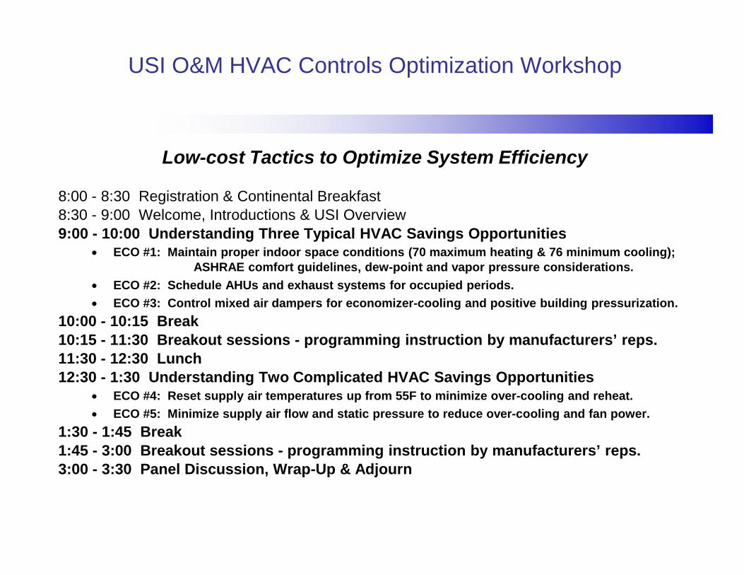
8:00 - 8:30 Registration & Continental Breakfast8:30 - 9:00 Welcome, Introductions & USI Overview9:00 - 10:00 Understanding Three Typical HVAC Savings Opportunities
• ECO #1: Maintain proper indoor space conditions (70 maximum heating & 76 minimum cooling); ASHRAE comfort guidelines, dew-point and vapor pressure considerations.
• ECO #2: Schedule AHUs and exhaust systems for occupied periods.• ECO #3: Control mixed air dampers for economizer-cooling and positive building pressurization.
10:00 - 10:15 Break10:15 - 11:30 Breakout sessions - programming instruction by manufacturers’ reps.11:30 - 12:30 Lunch 12:30 - 1:30 Understanding Two Complicated HVAC Savings Opportunities
• ECO #4: Reset supply air temperatures up from 55F to minimize over-cooling and reheat.• ECO #5: Minimize supply air flow and static pressure to reduce over-cooling and fan power.
1:30 - 1:45 Break1:45 - 3:00 Breakout sessions - programming instruction by manufacturers’ reps. 3:00 - 3:30 Panel Discussion, Wrap-Up & Adjourn
USI O&M HVAC Controls Optimization WorkshopHVAC ECO #1: 70-76 Thermostat Range
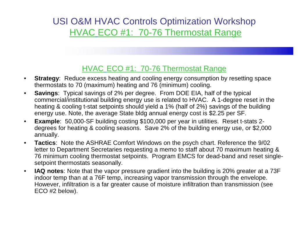
HVAC ECO #1: 70-76 Thermostat Range• Strategy: Reduce excess heating and cooling energy consumption by resetting space
thermostats to 70 (maximum) heating and 76 (minimum) cooling.• Savings: Typical savings of 2% per degree. From DOE EIA, half of the typical
commercial/institutional building energy use is related to HVAC. A 1-degree reset in the heating & cooling t-stat setpoints should yield a 1% (half of 2%) savings of the building energy use. Note, the average State bldg annual energy cost is $2.25 per SF.
• Example: 50,000-SF building costing $100,000 per year in utilities. Reset t-stats 2-degrees for heating & cooling seasons. Save 2% of the building energy use, or $2,000 annually.
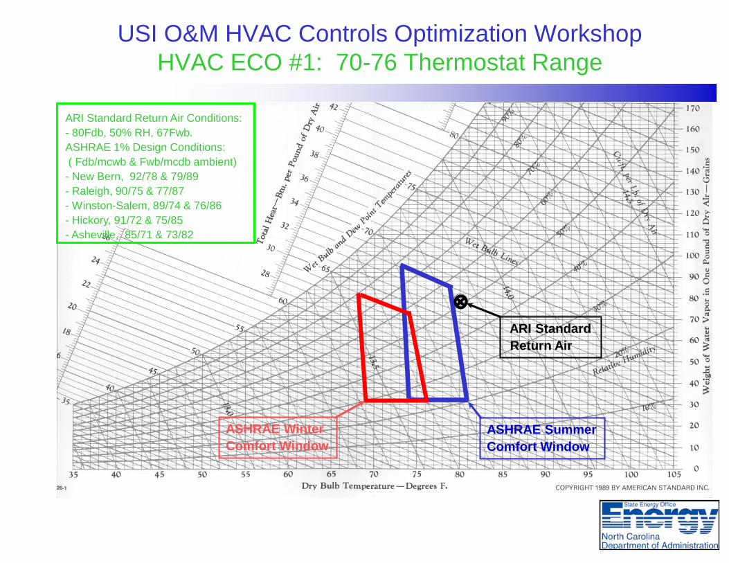
• Tactics: Note the ASHRAE Comfort Windows on the psych chart. Reference the 9/02 letter to Department Secretaries requesting a memo to staff about 70 maximum heating & 76 minimum cooling thermostat setpoints. Program EMCS for dead-band and reset single-setpoint thermostats seasonally.
• IAQ notes: Note that the vapor pressure gradient into the building is 20% greater at a 73F indoor temp than at a 76F temp, increasing vapor transmission through the envelope. However, infiltration is a far greater cause of moisture infiltration than transmission (see ECO #2 below).
USI O&M HVAC Controls Optimization WorkshopHVAC ECO #1: 70-76 Thermostat Range
ARI StandardReturn Air
ASHRAE SummerComfort Window
ASHRAE WinterComfort Window
ARI Standard Return Air Conditions:- 80Fdb, 50% RH, 67Fwb.ASHRAE 1% Design Conditions:( Fdb/mcwb & Fwb/mcdb ambient) - New Bern, 92/78 & 79/89- Raleigh, 90/75 & 77/87- Winston-Salem, 89/74 & 76/86- Hickory, 91/72 & 75/85- Asheville, 85/71 & 73/82
USI O&M HVAC Controls Optimization WorkshopHVAC ECO #2: Schedule Exhaust Fans
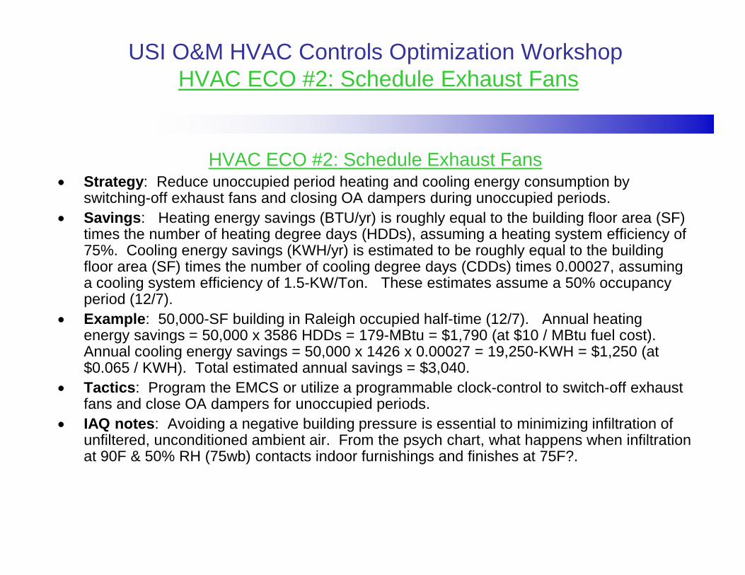
HVAC ECO #2: Schedule Exhaust Fans• Strategy: Reduce unoccupied period heating and cooling energy consumption by
switching-off exhaust fans and closing OA dampers during unoccupied periods.• Savings: Heating energy savings (BTU/yr) is roughly equal to the building floor area (SF)
times the number of heating degree days (HDDs), assuming a heating system efficiency of 75%. Cooling energy savings (KWH/yr) is estimated to be roughly equal to the building floor area (SF) times the number of cooling degree days (CDDs) times 0.00027, assuming a cooling system efficiency of 1.5-KW/Ton. These estimates assume a 50% occupancy period (12/7).
• Example: 50,000-SF building in Raleigh occupied half-time (12/7). Annual heating energy savings = 50,000 x 3586 HDDs = 179-MBtu = $1,790 (at $10 / MBtu fuel cost). Annual cooling energy savings = 50,000 x 1426 x 0.00027 = 19,250-KWH = $1,250 (at $0.065 / KWH). Total estimated annual savings = $3,040.
• Tactics: Program the EMCS or utilize a programmable clock-control to switch-off exhaust fans and close OA dampers for unoccupied periods.
• IAQ notes: Avoiding a negative building pressure is essential to minimizing infiltration of unfiltered, unconditioned ambient air. From the psych chart, what happens when infiltration at 90F & 50% RH (75wb) contacts indoor furnishings and finishes at 75F?.

USI O&M HVAC Controls Optimization WorkshopAnnual Heating and Cooling Degree Days for ECO #2
County Number County Name
Annual CDDs
Annual HDDs
County Number County Name
Annual CDDs
Annual HDDs
County Number County Name
Annual CDDs
Annual HDDs
County Number County Name
Annual CDDs
Annual HDDs
1 ALAMANCE 1292 3816 26 CUMBERLAN 1708 2851 51 JOHNSTON 1526 3140 76 RANDOLPH 1374 36202 ALEXANDER 979 4316 27 CURRITUCK 1542 3180 52 JONES 1678 2947 77 RICHMOND 1512 33443 ALLEGHANY 583 4988 28 DARE 1542 3180 53 LEE 1374 3140 78 ROBESON 1708 28514 ANSON 1512 3344 29 DAVIDSON 1374 3620 54 LENOIR 1678 2900 79 ROCKINGHA 1292 38165 ASHE 583 4988 30 DAVIE 1374 4141 55 LINCOLN 1512 3344 80 ROWAN 1374 36206 AVERY 682 4988 31 DUPLIN 1708 2900 56 MACON 781 4339 81 RUTHERFOR 1146 38417 BEAUFORT 1678 2947 32 DURHAM 1292 3816 57 MADISON 781 4339 82 SAMPSON 1708 29008 BERTIE 1542 3180 33 EDGECOMBE 1542 3180 58 MARTIN 1542 3180 83 SCOTLAND 1708 28519 BLADEN 1708 2851 34 FORSYTH 938 4141 59 MCDOWELL 781 4339 84 STANLY 1512 3344
10 BRUNSWICK 1708 2851 35 FRANKLIN 1417 3816 60 MECKLENBU 1512 3344 85 STOKES 938 440211 BUNCOMBE 781 4339 36 GASTON 1512 3344 61 MITCHELL 682 4339 86 SURRY 938 440212 BURKE 682 4316 37 GATES 1542 3180 62 MONTGOMER 1512 3344 87 SWAIN 781 433913 CABARRUS 1512 3344 38 GRAHAM 781 4339 63 MOORE 1512 3344 88 TRANSYLVAN 781 433914 CALDWELL 682 4316 39 GRANVILLE 1292 3816 64 NASH 1417 3180 89 TYRRELL 1542 318015 CAMDEN 1542 3180 40 GREENE 1678 2947 65 NEW HANOV 1708 2851 90 UNION 1512 334416 CARTERET 1678 2947 41 GUILFORD 1292 3816 66 NORTHAMPT 1542 3180 91 VANCE 1292 381617 CASWELL 1292 3816 42 HALIFAX 1417 3180 67 ONSLOW 1708 2851 92 WAKE 1526 314018 CATAWBA 1374 4316 43 HARNETT 1587 3140 68 ORANGE 1292 3816 93 WARREN 1292 381619 CHATHAM 1374 3620 44 HAYWOOD 781 4339 69 PAMLICO 1678 2947 94 WASHINGTO 1542 318020 CHEROKEE 781 4339 45 HENDERSON 781 4339 70 PASQUOTAN 1542 3180 95 WATAUGA 583 498821 CHOWAN 1542 3180 46 HERTFORD 1542 3180 71 PENDER 1708 2851 96 WAYNE 1678 290022 CLAY 781 4339 47 HOKE 1708 2851 72 PERQUIMAN 1542 3180 97 WILKES 583 498823 CLEVELAND 1146 3841 48 HYDE 1678 2947 73 PERSON 1292 3816 98 WILSON 1531 306424 COLUMBUS 1708 2851 49 IREDELL 1374 3620 74 PITT 1678 2947 99 YADKIN 938 414125 CRAVEN 1678 2947 50 JACKSON 781 4339 75 POLK 781 4339 100 YANCEY 781 4339

USI O&M HVAC Controls Optimization WorkshopHVAC ECO #2: Schedule Exhaust Fans
ARI StandardReturn Air
ASHRAE SummerComfort Window
ASHRAE WinterComfort Window
Note what happens when warm (90Fdb, 50% RH) infiltration contacts cool indoor finishes and furnishings:- infiltration cools,- RH increases towards saturation,- fungi amplify causing mildew,- IAQ deteriorates.

USI O&M HVAC Controls Optimization WorkshopHVAC ECO #3: 65F Economizer Setpoint
HVAC ECO #3: 65F Economizer Setpoint• Strategy: Reduce cooling energy consumption by using ambient air more often for free-
cooling.• Savings: Displacing 1,000-CFM of return air (at 65Fwb) with 60Fwb OA will reduce the
coil cooling load by 1.3-Tons (see the psych chart: 4.5 x 3.5 x 1000 / 12000 BTUs per Ton-hr = 1.3 Tons). In Raleigh, there are roughly 1,600 hours between 55 and 65F ambient (average 60F). Assuming a cooling system efficiency of 1.5-KW / Ton, roughly 3,000-KWHs could be saved annually (with a 24/7 building occupancy).
• Example: 50,000-SF building in Raleigh occupied half-time (12/7). Assume 1-CFM / SF or 50,000-CFM return airflow. Annual savings per 1,000-CFM is 3,000-KWHs (from above) for continuous occupancy (24/7), so divide by 2 for this building. Total estimated annual savings = 50 x 3,000 / 2 = 75,000-KWHs = $4,875 (at $0.065 / KWH).
• Tactics: Program the EMCS to increase the economizer setpoint to 65F ambient (without disabling the CHW valve between 55 and 65). If no mixed air damper controls are present, then provide damper operators, dry-bulb t-stats and programmable controller to fully-open OA dampers between 55 & 65F ambient (and modulate below 55 as needed for cooling).
• IAQ notes: Ensuring a positive building pressure is essential to minimizing infiltration of unfiltered, unconditioned ambient air. Introducing ventilation air at the AHU is preferable to infiltration. Refer to the above summer infiltration scenario.

USI O&M HVAC Controls Optimization WorkshopAnnual Hours Between 55 & 65 for ECO #3
Annual hours between 55 & 65Fdb ambient
Cherry Point 1,620
Elizabeth City 1,596
Goldsboro 1,536
Fayetteville 1,516
Raleigh 1,610
Greensboro 1,594
Charlotte 1,591

USI O&M HVAC Controls Optimization WorkshopHVAC ECO #3: 65F Economizer Setpoint
ARI StandardReturn Air
ASHRAE SummerComfort Window
ASHRAE WinterComfort Window
OA dampers open between 55& 65F- Assume present setpoint is 55F.-1610 hrs/yr between 55 & 65 Raleigh-1.3 Ton average load reduction per1000 CFM of RA displaced with OA.-3000 KWH / yr potential savings at1.5 KW/Ton cooling sys’m efficiency.
USI O&M HVAC Controls Optimization WorkshopHVAC ECO #4: Reset Supply Air Temperature
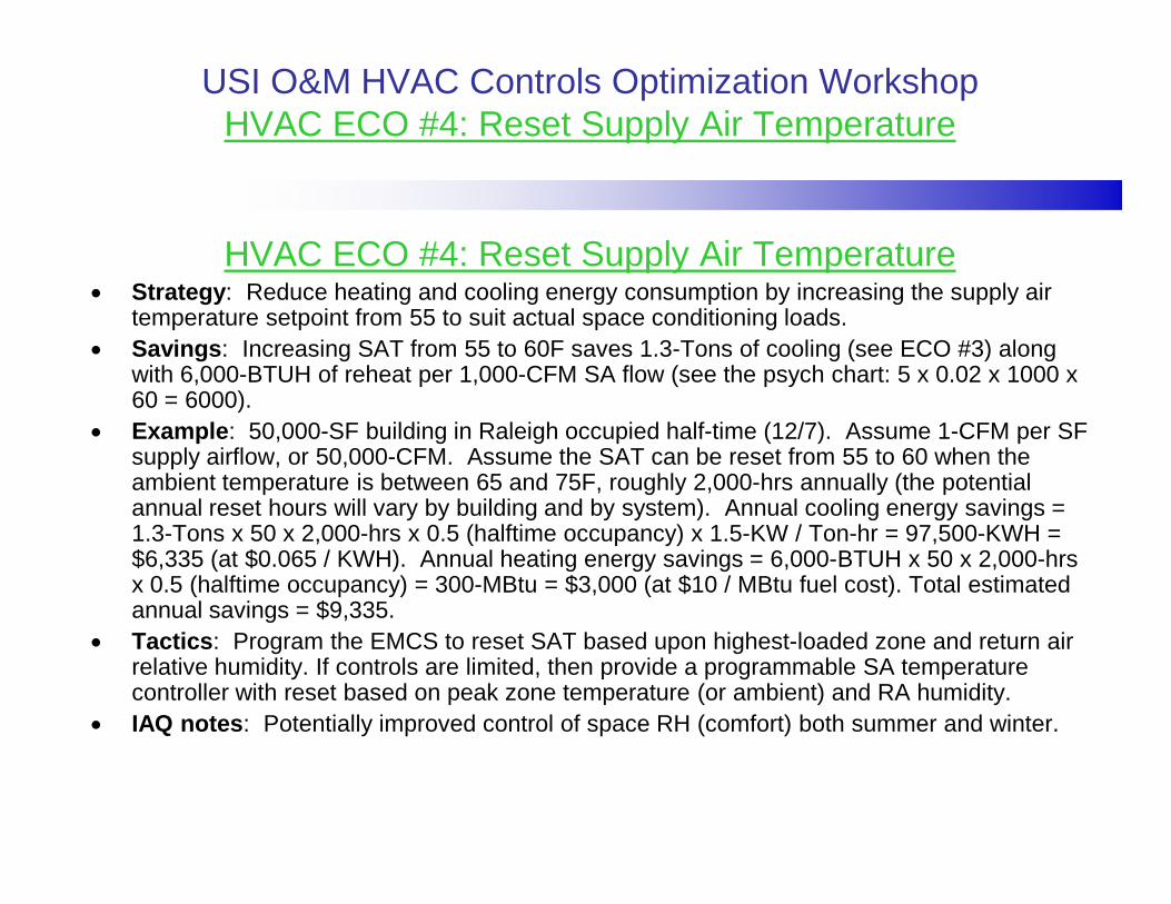
HVAC ECO #4: Reset Supply Air Temperature• Strategy: Reduce heating and cooling energy consumption by increasing the supply air
temperature setpoint from 55 to suit actual space conditioning loads.• Savings: Increasing SAT from 55 to 60F saves 1.3-Tons of cooling (see ECO #3) along
with 6,000-BTUH of reheat per 1,000-CFM SA flow (see the psych chart: 5 x 0.02 x 1000 x 60 = 6000).
• Example: 50,000-SF building in Raleigh occupied half-time (12/7). Assume 1-CFM per SF supply airflow, or 50,000-CFM. Assume the SAT can be reset from 55 to 60 when the ambient temperature is between 65 and 75F, roughly 2,000-hrs annually (the potential annual reset hours will vary by building and by system). Annual cooling energy savings = 1.3-Tons x 50 x 2,000-hrs x 0.5 (halftime occupancy) x 1.5-KW / Ton-hr = 97,500-KWH = $6,335 (at $0.065 / KWH). Annual heating energy savings = 6,000-BTUH x 50 x 2,000-hrs x 0.5 (halftime occupancy) = 300-MBtu = $3,000 (at $10 / MBtu fuel cost). Total estimated annual savings = $9,335.
• Tactics: Program the EMCS to reset SAT based upon highest-loaded zone and return air relative humidity. If controls are limited, then provide a programmable SA temperature controller with reset based on peak zone temperature (or ambient) and RA humidity.
• IAQ notes: Potentially improved control of space RH (comfort) both summer and winter.

USI O&M HVAC Controls Optimization WorkshopAnnual Hours Between 65 & 75 for ECO #4
Annual hours between 65 & 75Fdb ambient
Cherry Point 2,156
Elizabeth City 2,016
Goldsboro 2,100
Fayetteville 2,184
Raleigh 2,024
Greensboro 2,100
Charlotte 2,023

USI O&M HVAC Controls Optimization WorkshopHVAC ECO #4: Reset Supply Air Temperature
ARI StandardReturn Air
ASHRAE SummerComfort Window
ASHRAE WinterComfort Window
Reset Supply Air Temp from 55 to 60when ambient is between 65 & 75F.-2,000 hrs/yr between 65 & 75 Raleigh-Save 1.3-Tons cooling plus6000-BTUH reheat per 1000 CFM SA.-Save 97,500 KWH cooling plus 300-MBTU annually for 50% occ’y.

USI O&M HVAC Controls Optimization WorkshopHVAC ECO #5: Reduce Supply Air Flow and Fan Speed
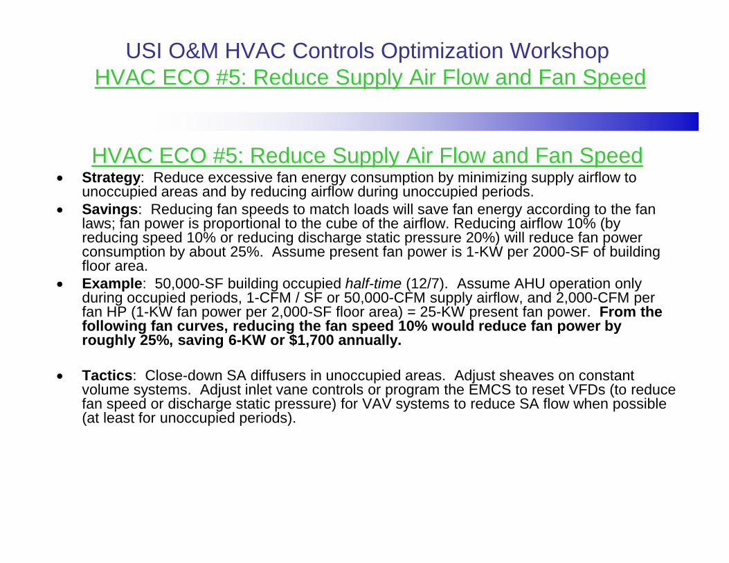
HVAC ECO #5: Reduce Supply Air Flow and Fan Speed• Strategy: Reduce excessive fan energy consumption by minimizing supply airflow to
unoccupied areas and by reducing airflow during unoccupied periods.• Savings: Reducing fan speeds to match loads will save fan energy according to the fan
laws; fan power is proportional to the cube of the airflow. Reducing airflow 10% (by reducing speed 10% or reducing discharge static pressure 20%) will reduce fan power consumption by about 25%. Assume present fan power is 1-KW per 2000-SF of building floor area.
• Example: 50,000-SF building occupied half-time (12/7). Assume AHU operation only during occupied periods, 1-CFM / SF or 50,000-CFM supply airflow, and 2,000-CFM per fan HP (1-KW fan power per 2,000-SF floor area) = 25-KW present fan power. From the following fan curves, closing-off SA dampers in unoccupied spaces to effectively reduce total SA flow by 10% would reduce fan power by only roughly 3% by riding the fan curve, saving 0.75-KW or 3,285-KWH or $215 annually.
• Tactics: Close-down SA diffusers in unoccupied areas. Adjust sheaves on constant volume systems. Adjust inlet vane controls or program the EMCS to reset VFDs (to reduce fan speed or discharge static pressure) for VAV systems to reduce SA flow when possible (at least for unoccupied periods).

USI O&M HVAC Controls Optimization WorkshopHVAC ECO #5: Reduce SA Flow and Fan Speed
Initial Operating Point
13.7-BHP

USI O&M HVAC Controls Optimization WorkshopHVAC ECO #5: Reduce Flow to Unoccupied Areas by 10%
New Operating Point
New 13.3-BHP is 3% less
22,500-CFM is 90% of initial flow
NEW
13.7-BHP at initial flow
USI O&M HVAC Controls Optimization WorkshopHVAC ECO #5: Reduce Supply Air Flow and Fan Speed
HVAC ECO #5: Reduce Supply Air Flow and Fan Speed• Strategy: Reduce excessive fan energy consumption by minimizing supply airflow to
unoccupied areas and by reducing airflow during unoccupied periods.• Savings: Reducing fan speeds to match loads will save fan energy according to the fan
laws; fan power is proportional to the cube of the airflow. Reducing airflow 10% (by reducing speed 10% or reducing discharge static pressure 20%) will reduce fan power consumption by about 25%. Assume present fan power is 1-KW per 2000-SF of building floor area.
• Example: 50,000-SF building occupied half-time (12/7). Assume AHU operation only during occupied periods, 1-CFM / SF or 50,000-CFM supply airflow, and 2,000-CFM per fan HP (1-KW fan power per 2,000-SF floor area) = 25-KW present fan power. From the following fan curves, reducing the fan speed 10% would reduce fan power by roughly 25%, saving 6-KW or $1,700 annually.
• Tactics: Close-down SA diffusers in unoccupied areas. Adjust sheaves on constant volume systems. Adjust inlet vane controls or program the EMCS to reset VFDs (to reduce fan speed or discharge static pressure) for VAV systems to reduce SA flow when possible (at least for unoccupied periods).

USI O&M HVAC Controls Optimization WorkshopHVAC ECO #5: Reduce Fan Speed 10%
13.7 BHP at full speed
10-BHP at 90% speed
Full speed fan curve
90% speed fan curve
NewOperatingPoint
SAME
USI O&M HVAC Controls Optimization WorkshopHVAC ECO #5: Reduce Supply Air Flow and Fan Speed
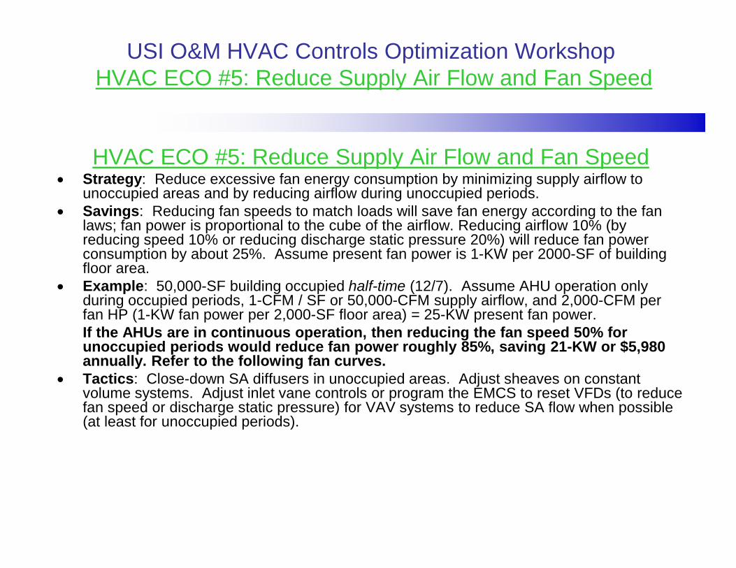
HVAC ECO #5: Reduce Supply Air Flow and Fan Speed• Strategy: Reduce excessive fan energy consumption by minimizing supply airflow to
unoccupied areas and by reducing airflow during unoccupied periods.• Savings: Reducing fan speeds to match loads will save fan energy according to the fan
laws; fan power is proportional to the cube of the airflow. Reducing airflow 10% (by reducing speed 10% or reducing discharge static pressure 20%) will reduce fan power consumption by about 25%. Assume present fan power is 1-KW per 2000-SF of building floor area.
• Example: 50,000-SF building occupied half-time (12/7). Assume AHU operation only during occupied periods, 1-CFM / SF or 50,000-CFM supply airflow, and 2,000-CFM per fan HP (1-KW fan power per 2,000-SF floor area) = 25-KW present fan power.If the AHUs are in continuous operation, then reducing the fan speed 50% for unoccupied periods would reduce fan power roughly 85%, saving 21-KW or $5,980 annually. Refer to the following fan curves.
• Tactics: Close-down SA diffusers in unoccupied areas. Adjust sheaves on constant volume systems. Adjust inlet vane controls or program the EMCS to reset VFDs (to reduce fan speed or discharge static pressure) for VAV systems to reduce SA flow when possible (at least for unoccupied periods).

USI O&M HVAC Controls Optimization WorkshopHVAC ECO #5: Reduce Fan Speed 50% for Unocc’d Periods
13.3 BHP at full speed
10-BHP at 90% speed
Full speed fan curve
90% speed fan curve
NewOperatingPoint
Initial Operating Point
1.7-BHP at 50% speed and flow
13.7-BHP at full speed
50% speed fan curve
Full speed fan curve
SAME

USI O&M HVAC Controls Optimization WorkshopHVAC ECO #5: Reduce Supply Air Flow and Fan Speed
HVAC ECO #5: Reduce Supply Air Flow and Fan Speed• Strategy: Reduce excessive fan energy consumption by minimizing supply airflow to
unoccupied areas and by reducing airflow during unoccupied periods.• Savings: Reducing fan speeds to match loads will save fan energy according to the fan
laws; fan power is proportional to the cube of the airflow. Reducing airflow 10% (by reducing speed 10% or reducing discharge static pressure 20%) will reduce fan power consumption by about 25%. Assume present fan power is 1-KW per 2000-SF of building floor area.
• Example: 50,000-SF building occupied half-time (12/7). Assume AHU operation only during occupied periods, 1-CFM / SF or 50,000-CFM supply airflow, and 2,000-CFM per fan HP (1-KW fan power per 2,000-SF floor area) = 25-KW present fan power.If the AHUs are in continuous operation, then closing inlet vanes to 25% for unoccupied periods to reduce flow 50% would reduce fan power roughly 50%, saving 12-KW or $3,400 annually.
• Tactics: Close-down SA diffusers in unoccupied areas. Adjust sheaves on constant volume systems. Adjust inlet vane controls or program the EMCS to reset VFDs (to reduce fan speed or discharge static pressure) for VAV systems to reduce SA flow when possible (at least for unoccupied periods).
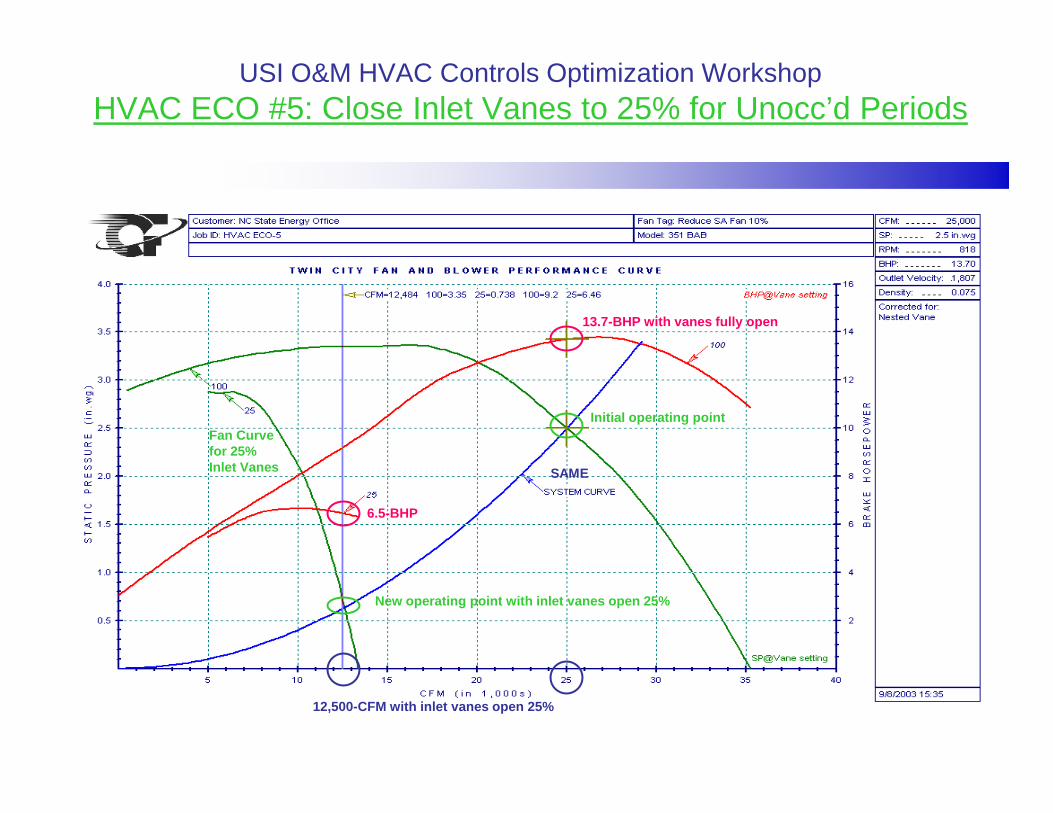
USI O&M HVAC Controls Optimization WorkshopHVAC ECO #5: Close Inlet Vanes to 25% for Unocc’d Periods
13.3 BHP at full speed
10-BHP at 90% speed
Full speed fan curve
90% speed fan curve
NewOperatingPoint
New operating point with inlet vanes open 25%
6.5-BHP
13.7-BHP with vanes fully open
Initial operating point
12,500-CFM with inlet vanes open 25%
Fan Curvefor 25%Inlet Vanes SAME