User Association in Massive MIMO HetNetsszm0001/papers/Yi_SystemJ_2017.pdf · 2020-04-13 · femtocell HetNet as a dynamic matching game and derived the optimal user association

IEEE SYSTEMS JOURNAL, VOL. 11, NO. 1, MARCH 2017 7

User Association in Massive MIMO HetNetsYi Xu, Student Member, IEEE, and Shiwen Mao, Senior Member, IEEE

Abstract—Massive multiple-input–multiple-output (MIMO) andsmall cell are both recognized as key technologies for the futurefifth-generation wireless systems. In this paper, we investigate theproblem of user association in a heterogeneous network (HetNet)with massive MIMO and small cells, where the macro base station(BS) is equipped with a massive MIMO, and the picocell BSsare equipped with regular MIMOs. We first develop centralizeduser association algorithms with proven optimality, consideringvarious objectives such as rate maximization, proportional fair-ness, and joint user association and resource allocation. We thendevelop a repeated game model, which leads to distributed userassociation algorithms with proven convergence to the Nash equi-librium. We demonstrate the efficacy of these optimal schemes bycomparing with several greedy algorithms through simulations.

Index Terms—Game theory, heterogeneous networks (HetNets),massive multiple input multiple output (MIMO), small cells, uni-modularity, user association.

I. INTRODUCTION

EXISTING and future wireless networks are facing thegrand challenge of a 1000-time increase in mobile data in

the near future [1]. To boost wireless capacity, two technologieshave gained most attention from both industry and academia.The first one is massive multiple input multiple output (MIMO;a.k.a., large-scale MIMO, full-dimension MIMO, or hyperMIMO) [2], [3]. The idea is to equip a base station (BS) withhundreds, thousands, or even tens of thousands of antennas,hereby providing an unprecedented level of degrees of freedom(DoFs) for mobile users. The massive MIMO concept hasbeen successfully demonstrated in recent studies [4], [5]. Thesecond technology is small cell, which is reshaping the future ofcellular networks [7]. A great benefit of deploying small cells isthat the distance of the user–BS link can be greatly shortened,leading to reduced transmit power, higher data rate, enhancedcoverage, and better spatial reuse of spectrum. Both massiveMIMO and small cells are recognized as key technologies ofthe future fifth-generation wireless systems [6].

In this paper, we consider a heterogeneous network (HetNet)with massive MIMO and small cells. Specifically, we considera HetNet where the macrocell BS (MBS) is equipped with amassive number of antennas and the picocell BSs (PBSs) areequipped with a regular amount of antennas. To fully harvest

Manuscript received December 20, 2014; revised May 16, 2015 and June 29,2015; accepted August 30, 2015. Date of publication September 22, 2015;date of current version March 10, 2017. This work was supported in part bythe National Science Foundation under Grant CNS-1247955 and Grant CNS-1320664 and in part by the Wireless Engineering Research and EducationCenter at Auburn University.

The authors are with the Department of Electrical and Computer Engi-neering, Auburn University, Auburn, AL 36849 USA (e-mail: [email protected]; [email protected]).

Digital Object Identifier 10.1109/JSYST.2015.2475702

the benefits promised by massive MIMO and small cells inan integrated HetNet system, it is critical to investigate theuser association problem, i.e., how to assign active users to theBSs such that the system-wide capacity can be maximized andusers’ experience can be enhanced.

There are already several recent studies moving forward inthis direction. In [8]–[11], the authors considered the problemof user association in massive MIMO systems operated inthe frequency-division duplexing mode. These papers focusedon a macrocell without small cells. In [12], user associa-tion in time-division duplexing (TDD) massive MIMO systemwas addressed, where fractional user association was allowed.Bayat et al. in [13] modeled the problem of user association in afemtocell HetNet as a dynamic matching game and derived theoptimal user association. In [14], near-optimal user associationschemes were proposed for HetNet with WiFi and conven-tional cellular networks. However, massive MIMO was notconsidered in these studies. In [15], the authors investigated theproblem of user association with conventional MIMO BSs andproposed a simple bias-based selection criterion to approximatemore complex selection rules. Björnson et al. [16] consideredimproving energy efficiency without sacrificing the quality ofservice of users in a massive MIMO and small cell HetNet.

Motivated by these interesting studies, we consider the userassociation problem in a TDD massive MIMO HetNet in thispaper. We take into consideration the practical constraints,such as the limited load capacity at each BS, without allowingfractional user association. The main goal is to maximizethe system capacity while enhancing user experience. Morespecifically, this paper contains two parts: centralized user as-sociation and distributed user association. For centralized userassociation, we investigate the problems of rate maximization,rate maximization with proportional fairness, and joint resourceallocation and user association. We prove the unimodularity ofour formulated problem and develop optimal user associationalgorithms to the problems of rate maximization and rate maxi-mization with proportional fairness. We then propose a seriesof primal decomposition and dual decomposition algorithmsto solve the problem of joint resource allocation and userassociation and prove the optimality of the proposed scheme.For distributed user association, we model the behavior and in-teraction between the service provider (who owns the BSs) andusers as repeated games. We consider two types of operations:1) the service provider sets the price and the users decide whichBS to connect to and 2) the users bid for connection opportu-nities. We prove that, in both cases, the proposed algorithmsconverge to the respective Nash equilibrium (NE).

In the remainder of this paper, Section II introduces thesystem model and preliminaries. Optimal centralized and dis-tributed user association schemes are presented in Sections III

1937-9234 © 2015 IEEE. Personal use is permitted, but republication/redistribution requires IEEE permission.See http://www.ieee.org/publications_standards/publications/rights/index.html for more information.

Authorized licensed use limited to: Auburn University. Downloaded on April 13,2020 at 02:19:45 UTC from IEEE Xplore. Restrictions apply.

8 IEEE SYSTEMS JOURNAL, VOL. 11, NO. 1, MARCH 2017

and IV, respectively. Section V presents the simulation study,and Section VI concludes this paper. Throughout this paper, aboldface upper (lower) case symbol denotes a matrix (vector),a normal symbol denotes a scalar, (·)H denotes the Hermitianof a matrix, and (·)T denotes the transpose of a matrix.

II. SYSTEM MODEL AND PRELIMINARIES

The system considered in this paper consists of K usersand J BSs inside a macro cell. There is a single MBS with amassive MIMO and (J − 1) PBSs, each with a regular amountof antennas. Following [19], the channel model we consideris hj,k,n = gj,k,nlj,k, where hj,k,n is the channel of antennan at BS j to user k, gj,k,n represents the small-scale fadingcoefficient between antenna n of BS j and user k, and lj,kstands for the large-scale fading coefficient between BS j anduser k. To obtain the channel vector hj,k between BS j anduser k, we could concatenate all the channel coefficients fromall the antennas of BS j as hj,k = [hj,k,1, hj,k,2, . . . , hj,k,n].For the channel coefficient matrix of signals transmitted fromBS j, we could obtain it by concatenating channel vector hj,k

as Hj = [hj,1,hj,2, . . . ,hj,k].Let yj denote the signals received by the users connecting to

BS j, Wj the precoding matrix of BS j, and dj the data sentfrom BS j. We have

yj = HjWjdj + nj (1)

where nj is the zero-mean circulant symmetric complexGaussian noise vector.

Each active user has the options to connect to either the MBSor a PBS. For a user k, define user association index variablexkj

as

xkj=

{1, if user k is connected to BS j

0, otherwise.(2)

Let the achievable rate of user k connecting to BS j be Rkj. We

define ηkj= xkj

Rkjand the overall data rate of user k to be

ηk, where

ηk =∑j

ηkj=

∑j

xkjRkj

. (3)

For users connecting to a massive MIMO BS j (i.e., the MBS),their achievable rate can be approximated with the followingdeterministic rate [12]:

Rkj= log

(1 +

Mj − Lj + 1

Lj

Pj lj,k1 +

∑j′ �=j Pj′ lj′,k

)(4)

where Mj is the number of antennas at the BS, Lj is theprefixed load parameter of the BS indicating how many usersit could serve, and Pj is the transmit power from the MBS.Note that there is no small-scale fading factor in (4). Thisapproximation has been proven to be accurate in [12].

As shown in [17], there are various sources of interferencesin a HetNet. However, among the PBSs, intercell interferencecoordination could be effectively performed according to [18].

We hereby ignore the intercell interference and only considerthe intracell interference. The achievable rate of a user kconnecting to PBS j can be then represented as follows:

R̃kj= log

⎛⎜⎝1 +Pj

∣∣∣hHj,kwj,k

∣∣∣21 +

∑k′ �=k Pj

∣∣∣hHj,kwj,k′

∣∣∣2⎞⎟⎠ (5)

where wj,k is the kth column of BS j’s precoding matrix Wj ,and | · | represents the absolute value. There are many precodingdesigns for conventional MIMO BSs, such as matched filter(MF) precoding, zero-forcing (ZF) precoding, and regularizedZF precoding [19]. Without loss of generality, we adopt MFprecoding with Wj = (1/

√ϕ)HH

j , where ϕ is a power nor-malization factor. The signal received by all the users connect-ing to PBS j can be rewritten as follows:

yj =

⎛⎜⎜⎝hHj,1hj,1d1 + hH

j,1hj,2d2 + · · ·+ hHj,1hj,kdk

hHj,2hj,1d1 + hH

j,2hj,2d2 + · · ·+ hHj,2hj,kdk

· · ·hHj,khj,1d1 + hH

j,khj,2d2 + · · ·+ hHj,khj,kdk

⎞⎟⎟⎠ . (6)

Thus, the achievable rate for user k with regard to PBS j can beobtained as follows:

ηkj= log

⎛⎜⎝1 +Pj

∣∣∣xkjhHj,khj,k

∣∣∣21 +

∑k′ �=k Pj

∣∣∣xk′jhHj,khj,k′

∣∣∣2⎞⎟⎠ . (7)

III. CENTRALIZED USER ASSOCIATION

Here, we consider the problem of centralized user asso-ciation. We assume that the BSs have all the channel stateinformation (CSI) via uplink training. We adopt the followingtwo utility functions for each user k with achievable rate ηk:

U(ηk) = ηk U(ηk) ={log(ηk), if ηk > 0

0, if ηk = 0.(8)

Maximizing the sum of the first utility yields the maximizationof the sum rate. Maximizing the sum of the second utility yieldsthe maximization of the geometric mean rate (i.e., achievingproportional fairness). Our goal is to maximize the systemutility by configuring the user–BS association.

A. Sum Rate Maximization

We first investigate the problem of maximizing the systemsum rate, i.e., with utility function U(ηk) = ηk. The problemcan be formulated as follows:

P1− 1 : max{xkj

}

K∑k=1

ηk

s.t.∑k

xkj≤ Lj ≤ Mj , j = 1, 2, . . . , J∑

j

xkj≤ 1, k = 1, 2, . . . ,K

Constraints (2), (3), (4), (7). (9)


XU AND MAO: USER ASSOCIATION IN MASSIVE MIMO HetNets 9

Note that the first constraint requires the number of usersconnecting to a BS to be no more than its prefixed load Lj ,which should, in turn, be no more than the number of antennasit has. This is because, theoretically, BS j can provide at mostMj DoFs. Assuming that the Lj are already chosen to satisfyLj ≤ Mj , we drop this constraint in the remainder of thispaper. The second constraint simply enforces that each user canconnect to at most one BS at a time.

A key observation is that, due to the binary xkj, if xkj

= 0,ηkj

= 0; if xkj= 1, ηkj

is a logarithm function. Thus, we canpull xkj

out of the log() function and rewrite (7) as

ηkj= xkj

log

⎛⎜⎝1 +Pj

∣∣∣hHj,khj,k

∣∣∣21 +

∑k′ �=k Pj


∣∣∣2⎞⎟⎠ . (10)

The R̃kjterm in (5) can be redefined as

R̃kj= log

⎛⎜⎝1 +Pj

∣∣∣hHj,khj,k

∣∣∣21 +

∑k′ �=k Pj


∣∣∣2⎞⎟⎠ . (11)

In (11), R̃kjalso depends on other users’ choices xk′

j, for

all k �= k′, as well. To make the problem tractable, we adoptthe worst case approximation by assuming that the users withinthe coverage of BS j (denoted by Gj ) all connect to BS j withperfect channels. This way, (11) can be approximated as

R̃kj= log

⎛⎜⎝1 +Pj

∣∣∣hHj,khj,k

∣∣∣21 + (|Gj | − 1)Pj

⎞⎟⎠ . (12)

Note here that |Z| stands for the absolute value. It also repre-sents the cardinality if Z is a set.

Define auxiliary variables ckjas follows:

ckj=

{Rkj

in (4), if BS j is the MBS

R̃kjin (12), if BS j is a PBS.

(13)

The sum rate maximization problem can be reformulated as

P1− 2 : max{xkj

}

K∑k=1

J∑j=1

xkjckj

s.t.∑k

xkj≤ Lj, j = 1, 2, . . . , J

∑j

xkj≤ 1, k = 1, 2, . . . ,K

Constraints (2), (13). (14)

Since the variables xkjare binary, problem P1− 2 falls into

the category of multiple knapsack problems, which is one ofthe 21 NP-complete problems of Karp [20]. Although a greedyalgorithm could be developed to compute suboptimal solutions,we show that problem P1− 2 can actually be optimally solvedby taking advantage of its special structure.

Let X be a matrix with entries xkj, k = 1, 2, . . . ,K ,

j = 1, 2, . . . , J . We first convert X to a vector x by con-catenating the rows of X and taking a transpose as x =[x11x21 , . . . , xK1

, . . . , x1J , . . . , xKJ]T and simplify the nota-

tion as x = [x1x2, . . . , xKJ]T . We then apply the same conver-

sion to the matrix comprising ckjand obtain vector c. Problem

P1− 2 can be rewritten as

P1− 3 : maxx

cTx

s.t.K∑

k=1

x(j−1)K+k ≤ Lj, j = 1, 2, . . . , J

J∑j=1

xk+(j−1)K ≤ 1, k = 1, 2, . . . ,K


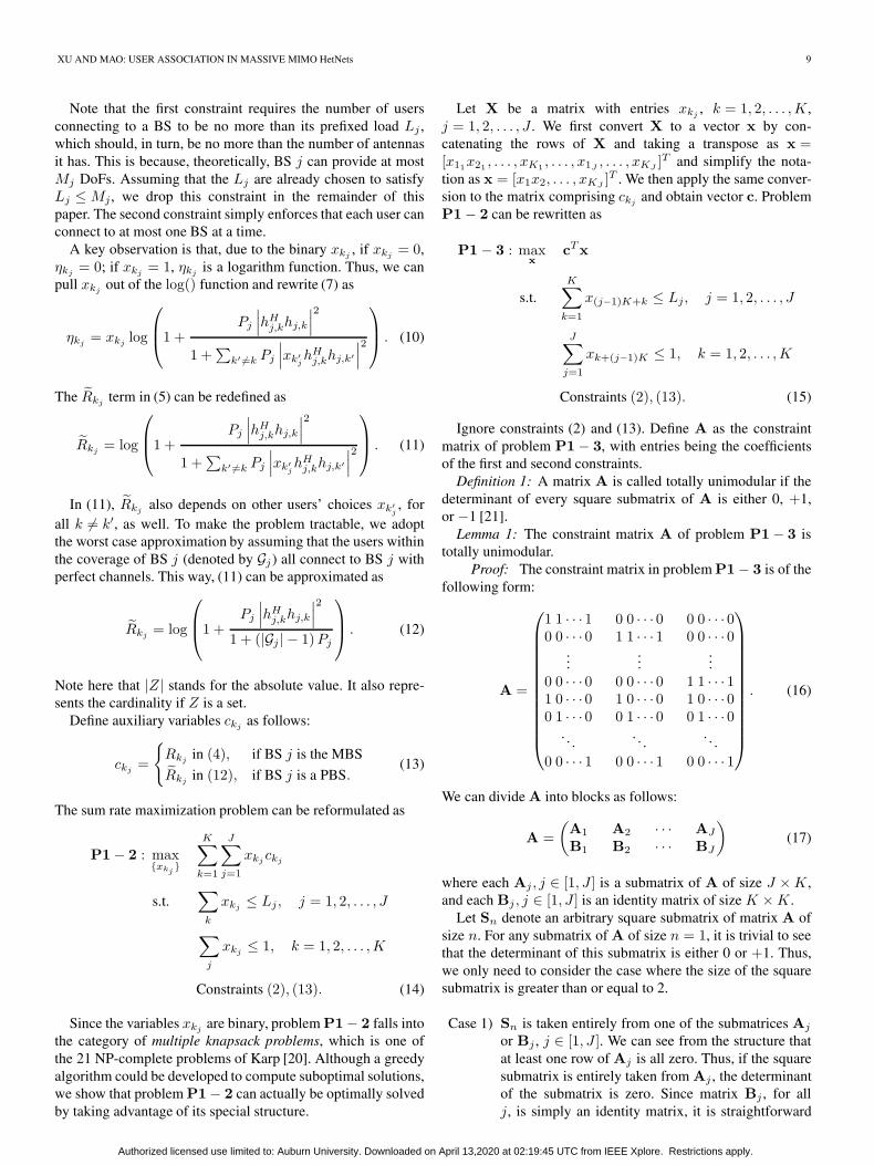
Ignore constraints (2) and (13). Define A as the constraintmatrix of problem P1− 3, with entries being the coefficientsof the first and second constraints.

Definition 1: A matrix A is called totally unimodular if thedeterminant of every square submatrix of A is either 0, +1,or −1 [21].

Lemma 1: The constraint matrix A of problem P1− 3 istotally unimodular.

Proof: The constraint matrix in problem P1− 3 is of thefollowing form:

A =

⎛⎜⎜⎜⎜⎜⎜⎜⎜⎜⎜⎜⎜⎝

1 1 · · · 1 0 0 · · · 0 0 0 · · · 00 0 · · · 0 1 1 · · · 1 0 0 · · · 0

......

...0 0 · · · 0 0 0 · · · 0 1 1 · · · 11 0 · · · 0 1 0 · · · 0 1 0 · · · 00 1 · · · 0 0 1 · · · 0 0 1 · · · 0

. . .. . .

. . .0 0 · · · 1 0 0 · · · 1 0 0 · · · 1

⎞⎟⎟⎟⎟⎟⎟⎟⎟⎟⎟⎟⎟⎠. (16)

We can divide A into blocks as follows:

A =

(A1 A2 · · · AJ

B1 B2 · · · BJ

)(17)

where each Aj , j ∈ [1, J ] is a submatrix of A of size J ×K ,and each Bj , j ∈ [1, J ] is an identity matrix of size K ×K .

Let Sn denote an arbitrary square submatrix of matrix A ofsize n. For any submatrix of A of size n = 1, it is trivial to seethat the determinant of this submatrix is either 0 or +1. Thus,we only need to consider the case where the size of the squaresubmatrix is greater than or equal to 2.

Case 1) Sn is taken entirely from one of the submatrices Aj

or Bj , j ∈ [1, J ]. We can see from the structure thatat least one row of Aj is all zero. Thus, if the squaresubmatrix is entirely taken from Aj , the determinantof the submatrix is zero. Since matrix Bj , for allj, is simply an identity matrix, it is straightforward



that the determinant of any square submatrix of Bj iseither 0 or +1.

Case 2) Sn is not entirely taken from any one of the subma-trices Aj or Bj , j ∈ [1, J ]. In this case, the squaresubmatrix must be taken from 2n (n = 1, . . . , J)submatrices of the submatrix set (Aj ∪Bj , j ∈1, . . . , J). We next proceed with our proof by apply-ing induction method.

For the base case n = 1, the square submatrix to be examinedis of size 2. Since the entries can be only 0 or +1, the deter-minant can be only 0,+1, or−1. Now, assuming that any squaresubmatrix of size (n−1) has determinant 0, +1, or −1, we needto check if the same conclusion holds for any square submatrixof size n.

We first notice that each column of A has exactly two +1 s.Moreover, exactly one of them is in Aj , and the other is in Bj .Let q∗ = argminq

∑i Sni,q

, where Sni,qis the (i, q)th entry of

Sn. That is, column q∗ has the minimum number of 1 s amongall the columns of Sn.

Let ζq∗ =minq∑

i Sni,q. ζq∗ can only be 0, 1, or 2. If ζq∗ =0,

then all the entries of the q∗th column of Sn are 0, which resultsin det(Sn) = 0, where det is short for determinant.

If ζq∗ = 1, then we could calculate det(Sn) by expandingthe q∗th column and obtain det(Sn) = det(S(n−1)). Sincedet(S(n−1)) is 0, 1, or −1 by our induction hypothesis, weconclude that det(Sn) is 0, 1, or −1.

If ζq∗ = 2, we could first negate all the entries taken from Bj

and then add all the rows in Bj to any nonzero row in Aj . Afterthis procedure, if that nonzero row in Aj is still nonzero, addthat row to any other nonzero row in Aj . Repeat this processuntil we get a zero row in Aj . This process always yields an all-zero row because we have equal number of +1 s in Aj and Bj .Since any basic row operation does not change the determinantand we finally get an all-zero row, we have det(Sn) = 0. Thatcompletes our induction. �

Fact 1: For a linear programming problem, if its constraintmatrix satisfies total unimodularity, then it has all integralvertex solutions [21].

Fact 2: For a linear programming problem, if it has feasibleoptimal solutions, then at least one of them occurs at a vertexof the polyhedron defined by its constraints [22].

Given the facts and Lemma 1, we have the following theo-rem. The proof is straightforward and omitted.

Theorem 1: The optimal solution of problem P1 can be ob-tained by solving a relaxed problem where the binary variablesxkj

are allowed to take real values between [0,1].With Theorem 1, we can obtain the optimal solution ofP1 by

solving the relaxed problem, termed NP1, using an LP solver[21] with an average complexity of O(J2K2).

B. Proportional Fairness

Here, we take proportional fairness among user achievablerates into consideration. The goal is to maximize

∑k U(ηk).

Since if ηk = 0 we define U(ηk) = 0, and negative utility willbe excluded from the maximization, we actually maximize

∑k max{log(

∑Jj=1 xkj

ckj), 0}. The problem can be formu-

lated as follows:

P2− 1 : max{xkj

}

K∑k=1

max

⎧⎨⎩log

⎛⎝ J∑j=1

xkjckj

⎞⎠ , 0

⎫⎬⎭s.t.

K∑k=1

xkj≤ Lj , j = 1, 2, . . . , J

J∑j=1

xkj≤ 1, k = 1, 2, . . . ,K

Constraints (2) (13). (18)

Problem P2− 1 is a nonlinear integer programming prob-lem, which is generally NP-hard. To get a better understandingof the problem, we examine its equivalent problem as follows:

P2− 2 : maxxkj

K∏k=1

⎛⎝ J∑j=1

xkjckj

⎞⎠s.t. same constraints as in (18). (19)

Problem P2− 2 is a geometric programming problem withbinary variables. The objective function is a polynomial func-tion with JK terms. Conventionally, to solve geometric pro-gramming problems, we need to introduce new variables suchas y = log(x) so that geometric programming can be solvedvia convex programming. However, here, xkj

are binary. Sincelog(0) = −∞, we could not apply these techniques. Anotherheuristic scheme is to first sort these JK coefficients and thenfind the Lj largest coefficients for each BS. However, even sort-ing these JK coefficients could be computationally prohibitiveeven for a small system, which requires O(JK log(JK))operations.

A key observation about the logarithm function is thatlog(

∑i τi) ≤

∑i log(τi), for all τi ≥ 2. Therefore, in prac-

tice,1 the optimal value of problem P2− 1 is upper boundedby that of the following problem:

NP2 : maxxkj

K∑k=1

J∑j=1

xkjlog(ckj

)

s.t. same constraints as in (18). (20)

We have the following results for the transformed problems.Lemma 2: Problems P2− 1 and NP2 are equivalent.

Proof: Recall that, if ηk = 0, we define U(ηk) = 0. Thesecond constraint

∑Jj=1 xkj

≤1 enforces that each user connect

to at most one BS. Consequently,max{log(∑J

j=1 xkjckj

), 0} =∑j xkj

log(ckj). Furthermore, we have

∑k

∑j xkj

log(ckj)=∑

k max{log(∑J

j=1 xkjckj

), 0}. Therefore, we conclude thatproblems P2− 1 and NP2 are equivalent. �

1Recall that ckjis the achievable rate of user k connecting to BS j. ckj

≥2

is generally satisfied in current wireless systems with a sufficiently largebandwidth and sufficiently high transmission power.



Comparing problem NP2 with P1− 2, we find that theyare equivalent as well. Thus, we can obtain the optimal value ofP2− 1 by applying the same technique used to solve problemP1− 2.

For comparison purposes, we propose two suboptimal greedyalgorithms, i.e., Algorithm 1 and Algorithm 2, as bench-marks. They can be directly used for comparison with problemP1− 1. Note that there are many other algorithms that canbe used to solve this problem, such as genetic algorithm [23]and swarm optimization [24]. However, these techniques havenot been applied in the context of mass MIMO systems. Wechose simple greedy algorithms to compare their performancewith the optimal solutions. To compare with problem P2− 1,in Algorithm 1, we need to change steps 7 and 8 as “while∃j, Lj �= 0 & maxk,j log(ck,j) > 0 do” and “Find (k∗, j∗) =argmaxk,j{log(ck,j)},” respectively. In Algorithm 2, we needto change steps 8 and 9 as “while Lj �= 0 & maxk log(ck,j) >0” and “Find (k∗, j) = argmaxk log(ck,j),” respectively.

The complexity of both greedy algorithms is O(KJ).

C. Joint Resource Allocation and User Association

Here, we take resource allocation into account. Consider amassive MIMO orthogonal frequency-division multiple access(OFDMA) HetNet. In OFDMA systems, such as long-termevolution, the time–frequency resource is divided into resourceblocks (RBs). A typical RB consists of 12 subcarriers (180 kHz)in the frequency domain and seven OFDMA symbols in thetime domain (0.5 ms). Thus, the system may have up to several

hundreds of RBs. We normalize it to be a unit number. A user kconnecting to a BS j gets a portion βkj

of the overall resource.The goal is to maximize the system utility considering bothresource allocation and user association.

Considering the logarithm rate utility and defining Φj ={k | xkj

= 1}, the problem is formulated as follows:

P3− 1 : max{xkj

,βkj}

K∑k=1

log

⎛⎝ J∑j=1

xkjckj

βkj

⎞⎠s.t.

∑k∈Φj

βkj≤ 1, j = 1, 2, . . . , J

J∑j=1

xkj≤ 1, k = 1, 2, . . . ,K∑

k∈Φj

βkj≤ 1, j = 1, 2, . . . , J


To solve problem P3− 1, we need to do the following: selectusers for each BS to serve and allocate resources to the asso-ciated users at each BS. We next propose a series of primaldecomposition and dual decomposition to optimally solve theproblem.

Due to binary variables xkjand real variables βkj

, problemP3− 1 is a mixed-integer nonlinear programming problem,which is generally NP-hard. However, next, we propose analgorithm to obtain its optimal solution.

Note that what we actually maximize is∑Kk=1 max{log(

∑Jj=1 xkj

ckjβkj

), 0}. For easier notation, theobjective function has been simplified. Since xkj

take binary

values and∑J

j=1 xkj≤1, we have

∑Kk=1log(

∑Jj=1 xkj

ckjβkj

)=∑Kk=1

∑Jj=1 xkj

log(ckjβkj

). Thus, problem P3− 1 can bereformulated as

P3− 2 : max{xkj

,βkj}

K∑k=1

J∑j=1

xkjlog

(ckj

βkj

)s.t. same constraints as problem P3− 1. (22)

The choices of βkjrely on the values of xkj

. Given thesecoupled variables, we first apply the primal decompositionmethod [25] to decompose problem P3− 2 into the followingtwo levels of problems. Fixing variables xkj

, we have the lowerlevel problem as

max{βkj

}

K∑k=1

J∑j=1

xkjlog

(ckj

βkj

)s.t.

∑k∈Φj

βkj≤ 1, j = 1, 2, . . . , J. (23)

When βkjare fixed, the higher level problem (or, the master

problem) is given by

max{xkj

}

K∑k=1

J∑j=1

xkjlog(ckj

βkj)

s.t. same constraints as problem P2− 1. (24)



Since there are no couplings among the subproblems, thelower level problem (23) can be further decomposed into Lsubproblems as follows:

max{βkj

}

K∑k=1

xkjlog(ckj

βkj)

s.t.K∑

k∈Φj

βkj≤ 1, j = 1, 2, . . . , J. (25)

Defining Lagrange multiplier λ, the Lagrangian of problem(25) is defined as

L =

K∑k=1

xkjlog(ckj

βkj) + λ

(1−

K∑k=1

βkj

). (26)

Applying Karush–Kuhn–Tucker conditions [26], the optimalsolution can be obtained as follows:

βkj=

xkj∑Kk=1 xkj

. (27)

Substituting (27) into the master problem, the objective func-tion becomes

K∑k=1

J∑j=1

xkjlog

(ckj∑K

k=1 xkj

). (28)

Note that we have dropped one xkjterm in (28), since, due to

the definition in (2), we have (xkj)2 = xkj

. Since∑K

k=1 xkjis

in the denominator, problem (28) has coupled objectives. Themain idea of addressing the coupled objective is to introduceauxiliary variables and additional equality constraints so thatthe coupling in the objective function is transferred to couplingin the constraint [25]. We thus introduce a new variable, whichis defined as

Ξj =

K∑k=1

xkj. (29)

To solve the aforementioned problem, we relax xkjto a real

number in [0, 1]. However, we will show later that, even ifwe have relaxed the variables, we could still find the optimalsolution to the original problem. The relaxed problem to besolved is

max{xkj

}

K∑k=1

J∑j=1

xkjlog

(ckj

Ξj

)s.t. Ξj ≤ Lj , j = 1, 2, . . . , J

J∑j=1

xkj≤ 1, k = 1, 2, . . . ,K

0 ≤ xkj≤ 1, for all k, j

Constraints (13), (29). (30)

Problem (30) is a convex optimization problem. DefiningLagrange multipliers for the equality constraints (29), problem

(30) can be solved with the dual decomposition method. Alter-natively, we propose Algorithm 3 to obtain the optimal solutionof problem (30) [10], [11], [27]. In Algorithm 3, δ(t) is the stepsize at the tth iteration given by

δ(t) =ϑ

t+ γ(31)

where ϑ and γ are positive numbers.Theorem 2: Algorithm 3 optimally solves problem (30).

Proof: Let x(t)k denote the solution produced by

Algorithm 3 at step t. Let ∂U(x(t)k ) be the subgradient of the

objective function in problem (30) at step t. It can be easilyverified that the updated direction in step 16 of Algorithm 3is the subgradient direction. Since Ξj is upper bounded by Lj

and K and∑K

k=1 xkjis upper bounded by K , ∂U(x(t)

k ) is alsobounded.

DenoteUa as the final result produced by Algorithm 3 and U∗

as the optimal solution of problem (30). We prove the theoremby contradiction. Assume that Ua is not optimal. Then theremust exist an ε > 0 such that Ua + 2ε < U∗. Then there mustbe a solution x̂k so that

Ua + 2ε < U(x̂k). (32)

Let t0 be sufficiently large so that, for any t > t0, we have

U(x(t)k

)≤ Ua + ε. (33)

Combining (32) and (33), we have U(x(t)k ) + ε < U(x̂k).

Let κ be a positive number that satisfies κ ≤inf{‖∂U(x(t)

k )‖}, for all t. It follows that∥∥∥x(t+1)k − x̂k

∥∥∥2 =∥∥∥x(t)

k − δ(t)∂U (t) − x̂k

∥∥∥2=

∥∥∥x(t)k − x̂k

∥∥∥2

+(δ(t)

)2 ∥∥∥∂U (t)∥∥∥2

− 2δ(t)(∂U (t)

)H (x(t)k − x̂k

)≥

∥∥∥x(t)k − x̂k

∥∥∥2

+(δ(t)

)2 ∥∥∥∂U (t)∥∥∥2

− 2δ(t)(U(x(t)k

)− U(x̂k)

)≥

∥∥∥x(t)k − x̂k

∥∥∥2

+(δ(t)

)2

κ2 + 2δ(t)ε

≥∥∥∥x(t)

k − x̂k

∥∥∥2

+ 2δ(t)ε ≥ · · ·

≥∥∥∥x(t0)

k − x̂k

∥∥∥2 + 2ε

t∑j=t0

δ(j). (34)

Note that the first inequality is due to the property of subgradi-ent. Thus, we finally have ‖x(t+1)

k − x̂k‖2 ≥ ‖x(t0)k − x̂k‖2 +

2ε∑t

j=t0δ(j), which cannot hold for sufficiently large t. Thus,

Algorithm 3 optimally solves problem (30). �



Theorem 3: The optimal solution to problem (30) is alsofeasible and optimal to problem (28).

Proof: From problem (28)–(30), the following change hasbeen applied:

xkj∈ B → xkj

∈ F (35)

where B = {0, 1} is set containing only 0 and 1, and F = [0, 1]is the set containing all the fractions from 0 to 1, inclusive of 0and 1. That is, we relax the variables from binary to real.

On one hand, since the set F contains much more numbersthan the set B, the optimal value to problem (30) provides anupper bound to that of problem (28). Denote the optimal utilityin (28) as U1 and the optimal utility in (30) as U2, we have

U2 ≥ U1. (36)

On the other hand, it can be observed from Algorithm 3 that

x(t)k∗j= 1 x

(t)k∗j= 0. (37)

That means that the solutions to problem (30) are 0 s and 1 s,which fall into B. Therefore, we have

U1 ≥ U2. (38)

With (37) and (38), we conclude that U1 = U2. Thus, al-though we transform problem (28) to problem (30), the optimalsolution is not affected by the transformation. �

To sum up, the optimal solution to problem (28) can besolved with Algorithm 3. For comparison purposes, we alsopropose two greedy algorithms as benchmarks, which are pre-sented in Algorithm 4 and Algorithm 5. The main idea of thegreedy algorithms is to first identify the most desirable user–BSpair and then to allocate all the resource to that user. This isrepeated until convergence is reached.

The complexity of both greedy algorithms is O(JK). Foreach iteration of Algorithm 3, the complexity is O(JK). Thus,the overall complexity of Algorithm 3 is higher than that ofAlgorithm 4 and Algorithm 5. However, we will show later thatthe complexity cost pays off. The optimal solution achieves agreat performance gain over the greedy algorithms.

IV. DISTRIBUTED USER ASSOCIATION

In the previous section, we assume a central controller thathas global information and assigns users to the BSs. Here, weconsider distributed user association. We still assume that theBSs have all the CSI via uplink training. We further assumethat all the BSs belong to the same service provider. Each usermakes its own decision based on the broadcast and local in-formation. Throughout this section, we do not allow fractionalconnection. We omit constraint (2) in the problem formulation,which is, however, enforced when solving the problem.

We model the behavior and interactions among the serviceprovider and users using repeated game theory. The first keyproblem is to determine whether the game will converge. Thesecond key problem is to analyze whether both sides are satis-factory about the outcome of the game, i.e., existence of the NE.

A. Service Provider Sets the Price

The players of the repeated game include the service providerand the users. During each round of the game, the serviceprovider determines the price of the connection service. The



users decide whether to connect, and if to connect, to whichBS. The strategy of the service provide is to set the price pkj

ofeach BS j for each user k, whereas the strategy of each user kis to set xkj

to either 0 or 1 for j ∈ J .The utility of the service provider is defined as UB =∑Kk=1

∑Jj=1 xkj

pkj. Since each BS is constrained by its max-

imum load capacity Lj , the service provider aims to solve thefollowing problem:

max{pkj

}UB =

K∑k=1

J∑j=1

xkjpkj

s.t.∑k

xkj≤ Lj, j = 1, 2, . . . , J. (39)

The utility of each user is the data rate achieved minus itspayment. Thus, each user aims to solve the following problem:

max{xkj

}Uk = max

⎧⎨⎩ωk log

⎛⎝ J∑j=1

xkjckj

⎞⎠−J∑

j=1

xkjpjk , 0

⎫⎬⎭s.t.

∑j

xkj≤ 1 (40)

where the logarithmic function represents the satisfaction levelof a user k toward its achievable rate, and ωk is a weight usedto tradeoff rate satisfaction and monetary payment. We assumethat the weightωk of each user is drawn from a finite set W with|W| elements. This assumption is true in real-world practice.For instance, $30 for a wireless service with a 60-Mb/s data rateis considered to be cheap, $45 is considered to be reasonable,$60 would be acceptable, $80 would be expensive for mostpeople, $100 would be too expensive, and $150 or above wouldnot be an option for most people. Thus, the weight of theusers has generally finite choices of values based on commonsense and is typically in a range = (0,WM ), where WM is themaximum possible value for ωk.

The repeated game is played as follows. Initially, the serviceprovider sets a price for each BS for each user and broadcaststhe prices to the users. Knowing the prices, the users willfeedback the service provider of their choices based on theirown calculations. Then, the service provider updates the pricesand broadcasts them to the users. Users again inform the serviceprovider of their choices, and so forth. The process is repeateduntil both the service provider and users are all satisfied withthe price.

Given the players and their strategies and utilities, we havethe following definition for the NE of the user association game.

Definition 2: A strategy set {p∗kj, x∗

kj}, for all k, j, is an NE

of the repeated game if UB(p∗kj, x∗

kj) ≥ UB(pkj

, x∗kj), for all

pkj, and Uk(p

∗kj, x∗

kj) ≥ Uk(p

∗kj, xkj

), for all k, xkj.

Due to the constraint that each user can only connect to oneBS, ωk log(

∑Jj=1 xkj

ckj) =

∑Jj=1 xkj

ωk log(ckj). Therefore,

the objective function of problem (40) becomes

Uk = max

⎧⎨⎩J∑

j=1

xkjωk log(ckj

)−J∑

j=1

xkjpjk , 0

⎫⎬⎭ . (41)

For the reformulated problem (41), the constraint∑

j xkj≤ 1

indicates that a user may choose not to connect to any of theBSs. On the other hand, if we restrict

∑j xkj

= 1, then, evenif the service provider sets the prices to infinity, each user willstill connect to a BS, which is clearly unreasonable.

Given the utility function (41) and the constraint in (40), theoptimal solution for each user can be derived as

j∗ = argmaxj∈J

[ωk log(ckj

)− pjk]

(42)

xkj=

{1, if j = j∗ and ωk log

(ck∗

j

)≥ pj∗k

0, otherwise.(43)

Such users’ decision can be interpreted this way. A user willchoose the best connection based on its own evaluation. If itsevaluation of the connection is greater than or equal to the price,it will connect to this BS. Otherwise, the user will not connectto the BS. Thus, we readily have the following result.

Lemma 3: The highest profit the service provider can obtainfrom a user k toward BS j is the user’s evaluation.

The service provider aims to solve problem (39) by tun-ing variables pkj

, k = 1, 2, . . . ,K , j = 1, 2, . . . , J . How-ever, the constraint

∑k xkj

≤ Lj is implicitly coupledwith all pkj

, since, according to the user’s choice, j∗ =

argmaxj∈J[ωk log(ckj

)− pjk]. The service provider prob-

lem is actually with the following form:

max{pkj

}UB =

K∑k=1

J∑j=1

xkjpkj

s.t.∑k

xkj(pkj)≤ Lj, j = 1, 2, . . . , J. (44)

Since problem (44) has coupling constraints, one may try tointroduce Lagrange multipliers to the constraint and solve theresulting problem using dual decomposition. However, sincepkj

is implicitly contained in the constraint, the gradient andsubgradient are difficult to find. Next, we propose Algorithm 6for the service provider and then prove that the algorithmachieves optimal utility for the service provider and the users.Note that, in Algorithm 6, |Fk| is the feedback size of user k.

Theorem 4: If the service provider adopts Algorithm 6, thegame converges, and the NE can be achieved.

Proof: We first notice that the service provider has pri-ority over the users. The users always make decisions basedupon the service provider’s price settings. Basically, the serviceprovider controls when the repeated game terminates.

In Algorithm 6, the service provider tests out the weightof each user using binary search with O(log2(|W|)) steps.Once the service provider obtains ωk, k = 1, 2, . . . ,K , it thenestimates the users’ price evaluation matrix V as follows:

vkj= ckj

ωk (45)

where vkjis the entry of matrix V at row j and column k.

Following Lemma 3, the service provider can obtain its optimal



price strategy by first selecting users for each BS and solvingthe following problem:

maxxkj

K∑k=1

J∑j=1

xkjvkj

s.t.∑k

xkj≤ Lj , j = 1, 2, . . . , J∑

j

xkj≤ 1, k = 1, 2, . . . ,K


The optimal solution x∗kj

to the preceding problem can besolved in a similar way as solving problem P1− 2. Then,the optimal prices for the service provider can be obtained asfollows:

p∗kj=

{vkj

, if x∗kj

= 1

vkj+ ε, otherwise

(47)

where ε is an arbitrary positive number.

Therefore, by adopting Algorithm 6, the optimal utility(highest) can be reached for the service provider. Meanwhile,we could see that all the users’ utility must be 0 due to theoptimal price setting (i.e., each user’s rate satisfaction matchesits monetary payment). That means that all the users achieve

the optimal utility given the price setting as well. Therefore, thegame converges to the NE. �

Note that it is possible that the optimal utility of the serviceprovider will be lower than the maximum utility during thegame, because the load capacity constraint may be violated dueto the distributed operation. The complexity of each iteration ofAlgorithm 6 is O(KJ).

B. User-Bidding-Based Approach

We next consider a bidding approach to the problem. Beforeservice starts, users bid to the service provider according totheir predicted satisfaction toward each BS. In addition, serviceprovider determines whether to accept a user’s bid and feedbackthe decisions to users. Then, the users make another roundof bids according to its predicted satisfaction and the serviceprovider’s decision history. The service provider again decideswhether to accept a user’s bid and feedback the decision, andso forth.

Assuming date-intensive users that strive for as high data rateas possible, each user solves the following problem:

max{pkj

}Uk = max

⎧⎨⎩J∑

j=1

xkjωk log(ckj

), 0

⎫⎬⎭s.t.

∑j

xkj(pkj) ≤ 1. (48)

On the other hand, the service provider aims to maximize itsutility, i.e., the total payment made by all the users, i.e.,

max{xkj

}UB =

K∑k=1

J∑j=1

xkjpkj

s.t.∑k

xkj≤ Lj , j = 1, 2, . . . , J. (49)

Note that the decision variables in these two problems aredifferent from those in problems (39) and (40), respectively.

We assume the general case that K ≥∑J

j=1 Lj (i.e., not allthe users can be served). In order to achieve the greatest levelof satisfaction, each user makes the highest possible payment.Thus, the optimal solution for each user is

pkj= max

⎧⎨⎩J∑

j=1

xkjωk log(ckj

), 0

⎫⎬⎭ . (50)

The optimal strategy for the service provider is summarized inAlgorithm 7.



During the first stage of the game, each user offers a price toits most desirable BS. Algorithm 7 is used to check if each BSj receives more than Lj bids. The service provider only puts Lj

top users on BS j’s waiting list based on the offered prices andrejects all other users. If BS j receives no more than Lj bids,all these users will be put on BS j’s waiting list.

At the second stage, if a user is in a BS’s waiting list, itwill keep on bidding the same BS with the same price toguarantee the highest utility. However, if a user gets rejectedin the previous round, as being selfish, it will exclude the BSsthat have rejected it and offers a price to its most desirable BSamong the remaining ones. For the service provider, it adoptsthe same strategy. If the number of bids received for a BSoutnumbers the load capacity of that BS, the service provideronly keeps the Lj most desirable users on the waiting list andrejects the others. It keeps all users on the waiting list if thenumber of offers received is less than a BS’s load capacity.These two stages repeat until convergence is achieved. Thecomplexity of each iteration of Algorithm 7 is O(J).

Lemma 4: The sequence of bids made by a user is nonin-creasing in the user’s preference list.

Proof: Before a user makes an offer, it computes thesatisfaction of all the BSs to obtain a preference list. Since auser aims to maximize its utility, it first proposes to the BSwith the highest satisfaction. If it is rejected by the BS, it willpropose to the BS with the second highest satisfaction, and soforth. Note that, even if a user may be on the waiting list of aBS, it may be removed from that waiting list at a later stage.If that happens, this user will start bidding to other BS. A userwill repeat this procedure until it is finally in a BS’s serving listor rejected by all BSs. This concludes the proof. �

Lemma 5: The sequence of bids a BS put on the waiting listis nondecreasing in its preference list.

Proof: Given the fact any BS has a finite load capacityand K ≥

∑Jj=1 Lj , all the BSs will have at least one user

bidding to it at some stage of the game. Since a BS aims tomaximize its utility, it puts all the users who make an offeron the waiting list. On the condition that there are too manyusers, it will reject the users who it will never serve. In thenext round of game, the BS will often have more or at leastthe same amount of bids compared with its current waiting list.This means that the BS has more choices. The BS again onlykeeps the most profitable ones and reject or remove the othersfrom the waiting list. Thus, the sequence of bids a BS put onthe list is nondecreasing in its preference list. �

Theorem 5: The repeated bidding game converges.Proof: We prove this theorem using contradiction as

follows. Based on Lemma 4 and Lemma 5, we prove thistheorem by contradiction. Suppose that this repeated game doesconverge. Then there must be a stage of the game that 1) thereis a user k and a BS j pair so that user k is connected to anotherBS j ′ or is not connected to any BS, 2) user k prefers BS j toBS j ′ or prefers to be not connected, and 3) BS j prefers user kto a user k′ who is on its serving list.

Consider the case where user k is served by BS j ′. Since thesequence of bids made by a BS is nondecreasing, it must bethe case that user k has never bidden to BS j during the game.Otherwise, if user k has bidden to BS j, BS j would not have

ended up with choosing k′ over k. In this case, user k wouldnever have bidden to BS j ′ either, since user k prefers j to j ′

and the bids (see Lemma 4). However, user k is now served byBS j ′, user k must have bidden to BS j ′, which contradicts thatuser k would never have bidden to BS j ′.

The same reasoning holds for the case when user k is notconnected to any BS. If BS j prefers k to k′ on the serving list,BS j would never reject user k while keeping user k′.

Therefore, the game converges when every user is either on awaiting list or has been rejected by every BS, and the game willconverge. �

From the proof, we can actually see that the game terminateswhen the least popular BS becomes fully loaded.

Theorem 6: The outcome of the repeated bidding game isoptimal for both the users and the service provider.

Proof: We prove this theorem using contradiction as fol-lows. Suppose that the outcome of the game is not optimal fora user k, who is connected to BS j. Then there must be anotherBS j ′, which has higher ranking than BS j in the preferencelist of user k and has a serving list of users {j ′1, j ′2, . . . , j ′Lj′

}.

Since BS j ′ serves these users, it means that BS j ′ prefers themto user k and BS j ′ is at the top of the preference lists of theseusers. If, at some stage, user k is in the waiting list of BS j (orit is inserted by force), the game must have not terminated.

Since user k is in the waiting list, then one of the final usersj ′1, j

′2, . . . , j

′Lj′

must be currently off the list, for example, user

j ′Lj′. Then user j ′Lj′

will immediately bid for BS j ′, since BS j ′

is at the top of its preference list among all the remaining BSs.In addition, BS j ′ will remove user k from its waiting list, sinceuser k has a lowest ranking in the preference list of BS j ′. Thus,when the repeated game terminates, the outcomes are optimalfor each user. It is obvious that the outcome is also optimal forthe service provider as well. �

From Theorem 5 and Theorem 6, we conclude that the gameconverges to the NE when the game terminates.

V. SIMULATION STUDY

We validate the proposed schemes with MATLAB simula-tions. The same random seeds were used for different algo-rithms for a fair comparison. For user location, we randomlygenerated their locations 1000 times. For each user generation,we randomly generate channel coefficients 2000 times. Thus,the result presented is the average of 2 000 000 simulations.

Throughout the simulations, we assume lj,k = 1/(1 +(dj,k/40)

3.5) for the path loss between a user and the massiveMIMO BS and lj,k = 1/(1 + (dj,k/40)

4) for the path lossbetween a user and a small cell BS [12]. We assume that thepower of small-scale fading follows a uniform distribution in[0.8,1]. We fix the location of the massive MIMO BS at thecenter of the cell. The other BSs are randomly placed acrossin the cell. Users are randomly placed in the area. The otherparameter settings are listed in Table I. The error bars in theplots are 95% confidence intervals.

Table II presents a comparison of rate maximization withthe optimal solution and the two proposed greedy algorithms.Table III shows a comparison of rate maximization consideringproportional fairness with the optimal solution and the two



TABLE ISYSTEM CONFIGURATION

TABLE IIRATE MAXIMIZATION OF CENTRALIZED CONTROL

TABLE IIILOG RATE UTILITY OF CENTRALIZED CONTROL

TABLE IVJOINT RESOURCE ALLOCATION AND USER ASSOCIATION

proposed greedy algorithms. We can see from both tables thatthe optimal solution achieves the highest network utility. Wealso notice that, as the number of users increases, the gapsbetween the optimal utility and the greedy solutions becomenarrower. This is because, as there are more users, the userdiversity effect becomes stronger. Thus, the greedy algorithmsand the optimal user association algorithm tend to produce sim-ilar solutions. Comparing greedy Algorithm 1 and Algorithm 2,we find that, in each step, Greedy Algorithm 1 always choosesthe globally best user–BS pair, whereas Greedy Algorithm 2chooses the best user for each BS sequentially. This is whyGreedy Algorithm 1 always achieves better performance thanGreedy Algorithm 2.

Table IV presents a comparison of the optimal joint resourceallocation and user association algorithm and the two proposedgreedy algorithms. We find that the optimal scheme achievesthe highest utility. Moreover, the gap between the optimalscheme and the greedy schemes is quite large. We also con-sider the equality constraint problem as a benchmark for thecomparison. For a fair comparison, we set the sum capacityof this system equal to the number of users. Thus, there are atotal of K = 50 active users in the system. The optimal solutionof problem P3− 2 achieves a network utility of −59.8462,whereas the optimal solution of problem (21) has a networkutility of 29.5433. We also found that if we connect every user,some edge users will be harmful for the network utility.

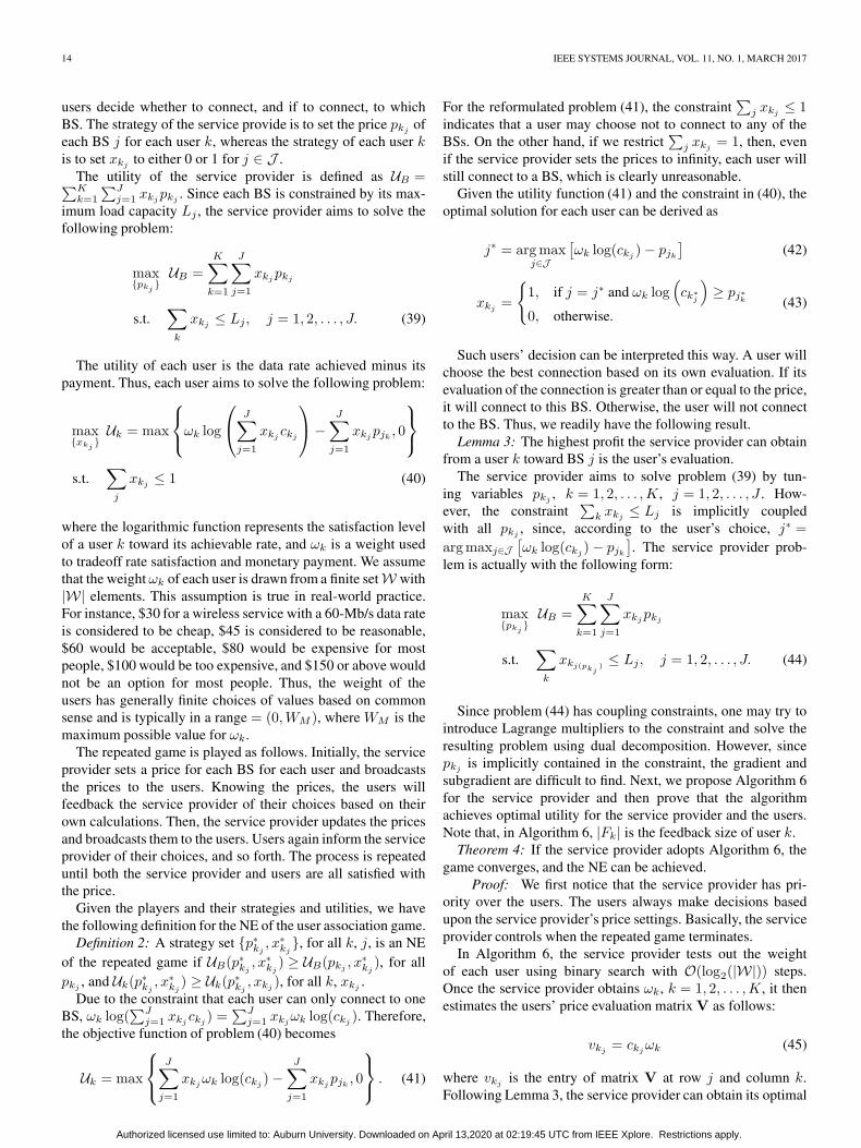
Fig. 1. Convergence of the repeated game when the service provider sets theprice and K = 100.

Fig. 2. Utility of the service provider, utility of the users, and the number ofrounds for convergence for systems with various numbers of users.

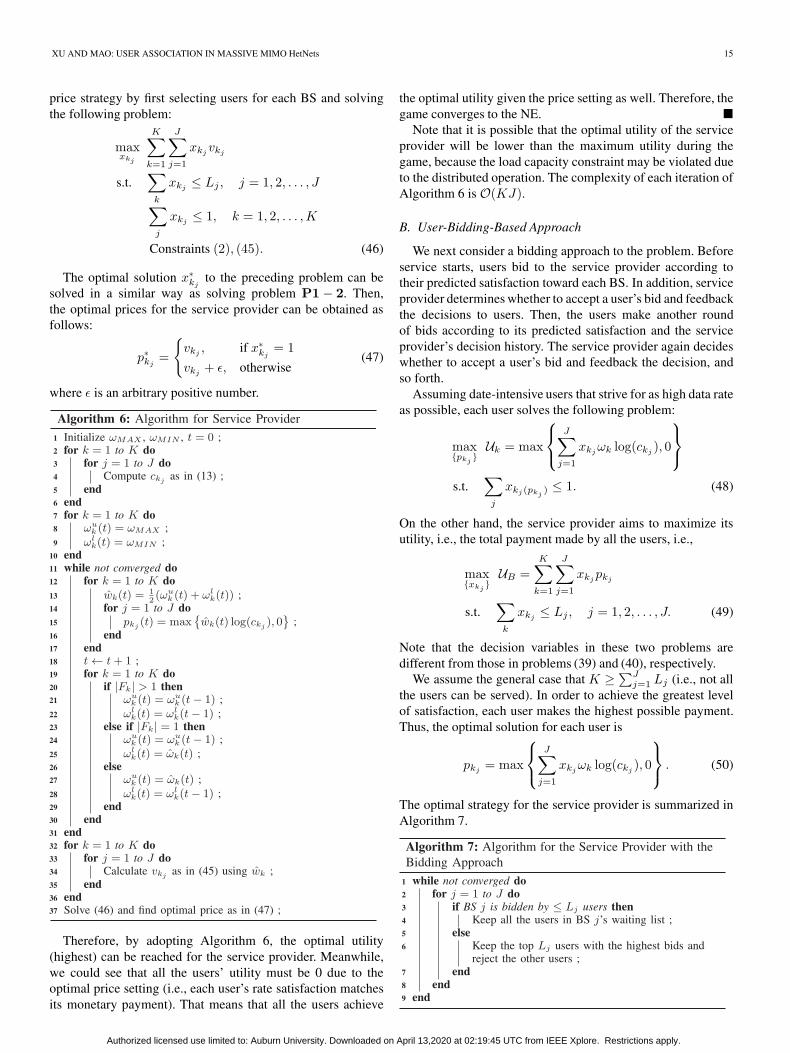
Fig. 1 shows the utility of the service provider and all userswhen the service provider sets the price (as in Section IV-A).It can be seen that the repeated game converges after eightrounds. Furthermore, the utility of all users is monotonicallydecreasing. That is because once a user’s evaluation is knownto the service provider, the service provider will set prices forthe highest profit, which results in 0 utility for that user. Asdiscussed, the utility for the service provider is not monoton-ically increasing, since, during the game, the load capacityconstraint may be violated. Since it is not the final result ofthe game, the capacity constraint could be violated for the timebeing. Since the loading capacity is violated, the utility of theservice provider could be very high. However, that actuallycould not be achieved after the game converges. Thus, the utilityafter the game converges could be lower than that during therepetition process of the game. Fig. 2 plots the utilities of theservice provider and users versus the number of users. Wecan see that, as the number of user increases, the utility ofthe service provider also increases. This is mainly due to theeffect of multiuser diversity. We can also observe that the gameterminates after about eight rounds no matter how many usersare active.



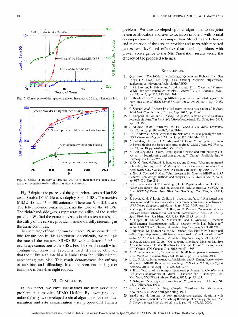
Fig. 3. Convergenceof the repeated game with respect toBSload when usersbid.

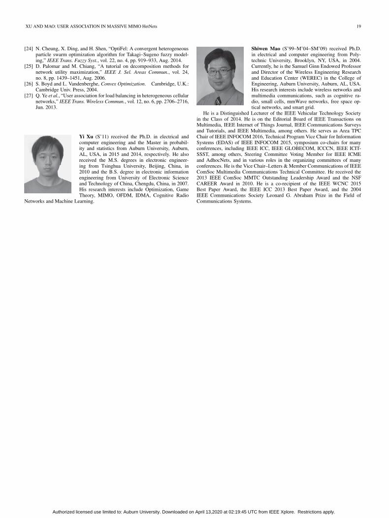
Fig. 4. Utility of the service provider with or without rate bias and conver-gence of the games under different numbers of users.

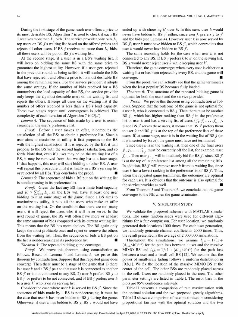
Fig. 3 depicts the process of the game when users bid for BSs(as in Section IV-B). Here, we deploy J = 41 BSs. The massiveMIMO BS has M = 400 antennas. There are K = 350 users.The left-hand-side y-axis represents the load of the 41 BSs.The right-hand-side y-axis represents the utility of the serviceprovider. We find the game converges in about ten rounds, andthe utility of the service provider is monotonically increasing asthe game continues.

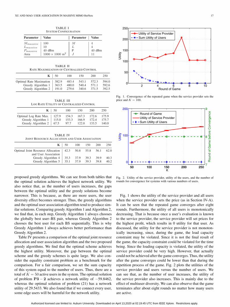
To encourage offloading from the macro BS, we consider ratebias for the BSs in this experiment. Specifically, we multiplethe rate of the massive MIMO BS with a factor of 0.5 toencourage connection to the PBSs. Fig. 4 shows the result whenconfiguration shown in Table I is used. It can be observedthat the utility with rate bias is higher than the utility withoutconsidering rate bias. This result demonstrates the efficacyof rate bias and offloading. It can be seen that both gamesterminate in less than eight rounds.

VI. CONCLUSION

In this paper, we have investigated the user associationproblem in a massive MIMO HetNet. By leveraging totalunimodularity, we developed optimal algorithms for rate max-imization and rate maximization with proportional fairness

problems. We also developed optimal algorithms to the jointresource allocation and user association problem with primaldecomposition and dual decomposition. Modeling the behaviorand interaction of the service provider and users with repeatedgames, we developed effective distributed algorithms withproven convergence to the NE. Simulation results verify theefficacy of the proposed schemes.

REFERENCES

[1] Qualcomm, “The 1000x data challenge,” Qualcomm Technol., Inc., SanDiego, CA, USA, Tech. Rep., 2014. [Online]. Available: https://www.qualcomm.com/invention/technologies/1000x

[2] E. G. Larsson, F. Tufvesson, O. Edfors, and T. L. Marzetta, “MassiveMIMO for next generation wireless systems,” IEEE Commun. Mag.,vol. 52, no. 2, pp. 185–195, Feb. 2014.

[3] F. Rusek et al., “Scaling up MIMO opportunities and challenges withvery large arrays,” IEEE Signal Process. Mag., vol. 30, no. 1, pp. 40–60,Jan. 2013.

[4] C. Shepard et al., “Argos: Practical many-antenna base stations,” in Proc.ACM MobiCom, Istanbul, Turkey, Aug. 2012, pp. 53–64.

[5] C. Shepard, H. Yu, and L. Zhong, “ArgosV2: A flexible many-antennaresearch platform,” in Proc. ACM MobiCom, Miami, FL, USA, Sep. 2013,pp. 163–165.

[6] J. Andrews et al., “What will 5G be?” IEEE J. Sel. Areas Commun.,vol. 32, no. 6, pp. 1065–1082, Jun. 2014.

[7] J. G. Andrews, “Seven ways that HetNets are a cellular paradigm shift,”IEEE Commun. Mag., vol. 51, no. 3, pp. 136–144, Mar. 2013.

[8] A. Adhikary, J. Nam, J.-Y. Ahn, and G. Caire, “Joint spatial divisionand multiplexing-the large-scale array regime,” IEEE Trans. Inf. Theory,vol. 59, no. 10, pp. 6441–6463, Oct. 2013.

[9] A. Adhikary and G. Caire, “Joint spatial division and multiplexing: Op-portunistic beamforming and user grouping.” [Online]. Available: http://arxiv.org/abs/1305.7252

[10] Y. Xu, G. Yue, N. Prasad, S. Rangarajan, and S. Mao, “User grouping andscheduling for large scale MIMO systems with two-stage precoding,” inProc. IEEE ICC, Sydney, NSW, Australia, Jun. 2014, pp. 5208–5213.

[11] Y. Xu, G. Yue, and S. Mao, “User grouping for Massive MIMO in FDDsystems: New design methods and analysis,” IEEE Access, vol. 2, no. 1,pp. 947–959, Sep. 2014.

[12] D. Bethanabhotla, O. Y. Bursalioglu, H. C. Papadopoulos, and G. Caire,“User association and load balancing for cellular massive MIMO,” inProc. IEEE Inf. Theory Appl. Workshop, San Diego, CA, USA, Feb. 2014,pp. 1–10.

[13] S. Bayat, R. H. Y. Louie, Z. Han, B. Vucetic, and Y. Li, “Distributed userassociation and femtocell allocation in heterogeneous wireless networks,”IEEE Trans. Commun., vol. 62, no. 8, pp. 3027–3043, Aug. 2014.

[14] Y. Zhang, D. Bethanabhotla, T. Hao, and K. Psounis, “Near-optimal user-cell association schemes for real-world networks,” in Proc. Inf. TheoryAppl. Workshop, San Diego, CA, USA, Feb. 2015, pp. 1–10.

[15] A. Gupta, H. Dhillon, S. Vishwanath, and J. Andrews, “Downlinkmulti-antenna heterogeneous cellular network with load balancing,”arXiv:1310.6795v2. [Online]. Available: http://arxiv.org/abs/1310.6795

[16] E. Björnson, M. Kountouris, and M. Debbah, “Massive MIMO and smallcells: Improving energy efficiency by optimal soft-cell coordination,”arXiv:1304.0553v3. [Online]. Available: http://arxiv.org/abs/1304.0553

[17] Y. Xu, S. Mao, and X. Su, “On adopting Interleave Division MultipleAccess to two-tier femtocell networks: The uplink case,” in Proc. IEEEICC, Ottawa, ON, Canada, Jun. 2012, pp. 591–595.

[18] A. Damnjanovic et al., “A survey on 3GPP heterogeneous networks,”IEEE Wireless Commun. Mag., vol. 18, no. 3, pp. 10–21, Jun. 2011.

[19] L. Lu, G. Li, A. Swindlehurst, A. Ashikhmin, and R. Zhang, “An overviewof massive MIMO: Benefits and challenges,” IEEE J. Sel. Topics SignalProcess., vol. 8, no. 5, pp. 742–758, Oct. 2014.

[20] R. Karp, “Reducibility among combinatorial problems,” in Complexity ofComputer Computations, R. Miller, J. Thatcher, and J. Bohlinger, Eds.New York, NY, USA: Springer-Verlag, 1972, pp. 85–103.

[21] A. Schrijver, Theory of Linear and Integer Programming. Hoboken, NJ,USA: Wiley, Jun. 1998.

[22] C. Berenstein and R. Gay, Complex Variables: An Introduction.New York, NY, USA: Springer-Verlag, 1997.

[23] Yandra and H. Tamura, “A new multiobjective genetic algorithm withheterogeneous population for solving flowshop scheduling problems,” Int.J. Comput. Integr. Manuf., vol. 20, no. 5, pp. 465–477, Jul. 2007.



[24] N. Cheung, X. Ding, and H. Shen, “OptiFel: A convergent heterogeneousparticle swarm optimization algorithm for Takagi–Sugeno fuzzy model-ing,” IEEE Trans. Fuzzy Syst., vol. 22, no. 4, pp. 919–933, Aug. 2014.

[25] D. Palomar and M. Chiang, “A tutorial on decomposition methods fornetwork utility maximization,” IEEE J. Sel. Areas Commun., vol. 24,no. 8, pp. 1439–1451, Aug. 2006.

[26] S. Boyd and L. Vandenberghe, Convex Optimization. Cambridge, U.K.:Cambridge Univ. Press, 2004.

[27] Q. Ye et al., “User association for load balancing in heterogeneous cellularnetworks,” IEEE Trans. Wireless Commun., vol. 12, no. 6, pp. 2706–2716,Jun. 2013.

Yi Xu (S’11) received the Ph.D. in electrical andcomputer engineering and the Master in probabil-ity and statistics from Auburn University, Auburn,AL, USA, in 2015 and 2014, respectively. He alsoreceived the M.S. degrees in electronic engineer-ing from Tsinghua University, Beijing, China, in2010 and the B.S. degree in electronic informationengineering from University of Electronic Scienceand Technology of China, Chengdu, China, in 2007.His research interests include Optimization, GameTheory, MIMO, OFDM, IDMA, Cognitive Radio

Networks and Machine Learning.

Shiwen Mao (S’99–M’04–SM’09) received Ph.D.in electrical and computer engineering from Poly-technic University, Brooklyn, NY, USA, in 2004.Currently, he is the Samuel Ginn Endowed Professorand Director of the Wireless Engineering Researchand Education Center (WEREC) in the College ofEngineering, Auburn University, Auburn, AL, USA.His research interests include wireless networks andmultimedia communications, such as cognitive ra-dio, small cells, mmWave networks, free space op-tical networks, and smart grid.

He is a Distinguished Lecturer of the IEEE Vehicular Technology Societyin the Class of 2014. He is on the Editorial Board of IEEE Transactions onMultimedia, IEEE Internet of Things Journal, IEEE Communications Surveysand Tutorials, and IEEE Multimedia, among others. He serves as Area TPCChair of IEEE INFOCOM 2016, Technical Program Vice Chair for InformationSystems (EDAS) of IEEE INFOCOM 2015, symposium co-chairs for manyconferences, including IEEE ICC, IEEE GLOBECOM, ICCCN, IEEE ICIT-SSST, among others, Steering Committee Voting Member for IEEE ICMEand AdhocNets, and in various roles in the organizing committees of manyconferences. He is the Vice Chair–Letters & Member Communications of IEEEComSoc Multimedia Communications Technical Committee. He received the2013 IEEE ComSoc MMTC Outstanding Leadership Award and the NSFCAREER Award in 2010. He is a co-recipient of the IEEE WCNC 2015Best Paper Award, the IEEE ICC 2013 Best Paper Award, and the 2004IEEE Communications Society Leonard G. Abraham Prize in the Field ofCommunications Systems.


Documents

User Association in Massive MIMO HetNetsszm0001/papers/Yi_SystemJ_2017.pdf · 2020-04-13 · femtocell HetNet as a dynamic matching game and derived the optimal user association