USA · Range of Oregon, USA ... (Noss, 1983; Harris, 1984 ... natural forest matrix were digitally recorded as polygons for both the 1972 and 1987 data

Biolo_icctl Conservation 57 { 199 l ) 73-88 N95- 24096

Measuring Forest Landscape Patterns in the Cascade

Range of Oregon, USA

William J. Ripple

Environmental Remote Sensing Applications Laboratory, Department of Forest Resources.

Oregon State University, Corvallis, Oregon 97331, USA

G. A. Bradshaw

Environmental Remote Sensing Applications Laboratory and Department of Forest Science.

Oregon State University, Corvallis, Oregon 97331, USA

&

Thomas A. Spies

USDA Forest Service, Pacific Northwest Research Station and

Oregon State University, Corvallis, Oregon 97331. USA

{Received 24 April 1990; revised version received and accepted 8 October 1990)

.->

- 5 --._

(/i

]/y,/ _'

A BSTRA CT

This paper describes the use of a set of spatial statistics to quantify the

landscape pattern caused by the patchwork of clearcuts made over a 15-year

period in the western Cascades of Oregon. Fifteen areas were selected at

random to represent a diversity of landscape fragmentation patterns.

Managed forest stands (patches) were digitized and analysed to produce both

tabular and mapped information describing patch size, shape, abundance and

spacing, and matrix characteristics of a given area. In addition, a GIS

fragmentation index was developed which was found to be sensitive to patch

abundance and to the spatial distribution of patches. Use of the GIS-derived

index provides an automated method of determining the level of forest

fragmentation and can be used to facilitate spatial analysis of the landscape

for later coordination with field and remotely sensed data. A comparison of

the spatial statistics calculated for the two years indicates an increase in forest

fragmentation as characterized by an increase in mean patch abundance and a

decrease in interpatch distance, amount of interior natural forest habitat, and

73

Biol. Conserv. 0006-3207/91/$03"50 © 1991 Elsevier Science Publishers Ltd, England. Printedin Great Britain

https://ntrs.nasa.gov/search.jsp?R=19950017676 2018-07-10T09:32:43+00:00Z

74 William J. Ripple, G. A. Bradshaw, Thomas A. Spies

the GIS fragmentation index. Such statistics capable of quantifying patch

shape and spatial distribution may prove important in the evaluation of the

changing character of interior and edge habitats for wildlife.

INTRODUCTION

The Douglas-fir Pseudotsuga menziesii (Mirb.) Franco forests of western

Oregon have been cut extensively during the past 40 years. In these forests,clearcuts, new plantations, and second-growth stands now exist on the

landscape formerly dominated by extensive old-growth forests and younger

forests resulting from fire disturbance (Spies & Franklin, 1988). Con-

sequently, the landscape has become more spatially heterogeneous. Some ofthe effects of this newly created landscape on the forest ecosystem are

immediately apparent. For example, the amount of old-growth foresthabitat for interior species such as the northern spotted owl Strix

occidentalis caurina is altered with forest harvesting practices. Less well

understood are the long-term and more subtle interactive effects on

ecosystem processes (e.g. changes in species diversity and abundance,

nutrient cycling and primary forest productivity), which may occur as aresult of the changed forest mosaic. It is generally accepted that wildlife

ecology and behavior may be strongly dependent on the nature and patternof landscape elements (Forman & Godron, 1986), but few precisemeasurements relating these changes to landscape spatial alteration have

been made. Properties of forested landscapes such as patch size, the amount

of edge, the distance between habitat areas, and the connectedness of habitat

patches have a direct influence on the flora and fauna (Thomas, 1979; Harris,1984; Franklin & Forman, 1987; Ripple & Luther, 1987). For these reasons,models and monitoring schemes are urgently needed for prescribing the

location, size, and shape of future harvest units and old-growth habitat

patches. With proper design, these forest landscapes should be able toachieve desired habitat values and maintain biological diversity (Noss, 1983;

Harris, 1984; Franklin & Forman, 1987).As a first step to studying forest landscape pattern, the spatial character of

the landscape must be quantified to relate ecological processes to landscape

configuration. Numerous methods and indices have been proposed for these

purposes (e.g. Forrnan & Godron, 1986; Milne, 1988; O'Neill et al., 1988).Landscape pattern can be quantified using statistics in terms of the

landscape unit itself (e.g. patch size, shape, abundance, and spacing) as well

as the spatial relationship of the patches and matrix comprising the

landscape (e.g. nearest-neighbor distance and amount of contiguous matrix).A selection of these measures can therefore describe the several aspects of

fragmentation which occur as the result of forest harvesting practices.

Forest landscape patterns in Oregon 75

Because spatial analyses are often cumbersome due to large amounts ofdata, it is desirable that the analysis be automated. Furthermore, it should be

amenable for study at various scales in concert with a variety of data types.

Automated systems such as geographical information systems (GIS) address

such needs (Ripple, 1987, 1989). With the development of GIS, the ability to

readily measure spatial characteristics of landscapes in conjunction with

field and remotely sensed data has become possible.

The overall goal of the present study was to test the feasibility of

measuring forest landscape patterns accurately using a set of spatial

statistics and a GIS. Specifically, we set out to apply a set of statistics to a

series of forested landscapes in the Cascade Range of western Oregon to (t)

assess the sensitivity of these statistics to characterize landscape pattern: (2)

develop and test a GIS-derived index to measure fragmentation: and (3)

quantify the change and types of forest fragmentation through time in our

study area. The results of this pilot study are intended to aid the forester,

wildlife biologist, and land manager in assessing change in wildlife habitat

and alteration in ecosystem processes as a result of forest fragmentation.

STUDY AREA

The study area consisted of the Blue River and Sweet Home ranger districts

of the Willamette National Forest. According to Franklin and Dyrness

(1973), these ranger districts lie primarily in the western hemlock Tsuga

heterophylla and pacific silver fir Abies amabilis vegetation zone, with the

major forest tree species consisting of Douglas-fir, western hemlock, pacific

silver fir, noble fir Abies procera, and western redcedar Thuja plicata. The

climate can be characterized as maritime with wet, mild winters and dry,

warm summers. Under natural conditions, Douglas-fir is the seral dominant

at elevations below 1000 m, where it typically develops nearly pure, even-

aged stands after fire. Large areas are covered by old-growth Douglas-fir/

western hemlock forests in which Douglas-firs are over 400 years old. Fires

during the past 200 years have created a complex mosaic of relatively even-aged natural stands throughout the study area. Superimposed on this

natural mosaic is a second component of pattern complexity resulting from

timber harvesting over the last 40 years.

METHODS

Data acquisition

Landscapes were classified in terms of managed and natural elements.

Managed forest stands (typically young forest plantations of up to


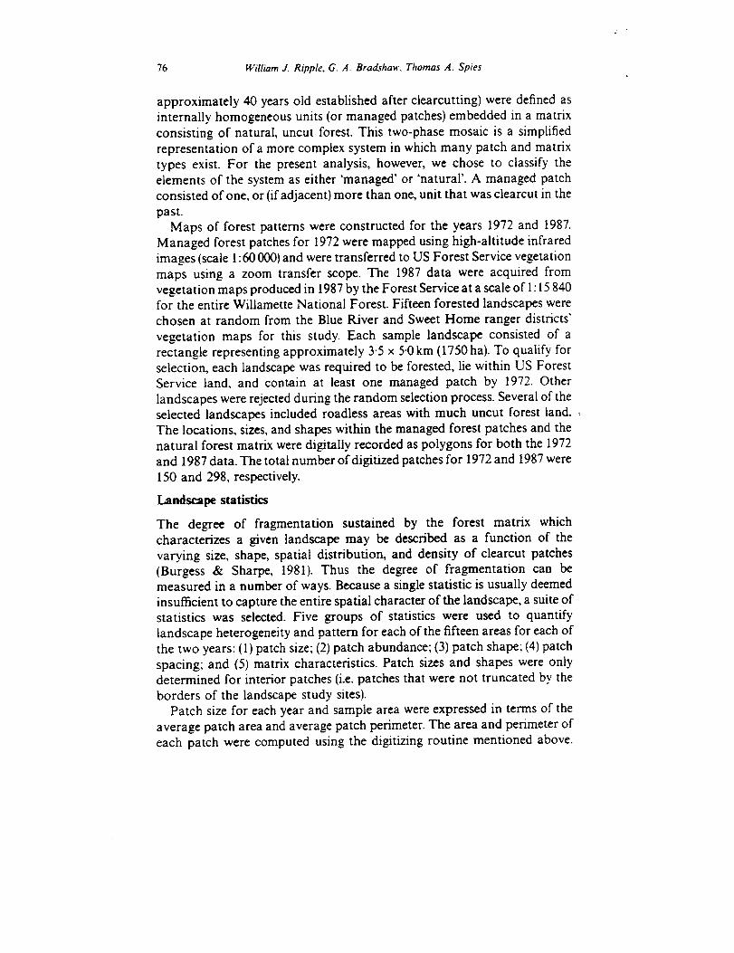
approximately 40 years old established after clearcutting) were defined as

internally homogeneous units (or managed patches) embedded in a matrix

consisting of natural, uncut forest. This two-phase mosaic is a simplified

representation of a more complex system in which many patch and matrix

types exist. For the present analysis, however, we chose to classify the

elements of the system as either 'managed' or 'natural'. A managed patch

consisted of one, or (if adjacent) more than one, unit that was clearcut in the

past.Maps of forest patterns were constructed for the years 1972 and 1987.

Managed forest patches for 1972 were mapped using high-altitude infrared

images (scale 1: 60 000) and were transferred to US Forest Service vegetation

maps using a zoom transfer scope. The 1987 data were acquired from

vegetation maps produced in 1987 by the Forest Service at a scale of 1:15 840for the entire Willamette National Forest. Fifteen forested landscapes were

chosen at random from the Blue River and Sweet Home ranger districts'

vegetation maps for this study. Each sample landscape consisted of a

rectangle representing approximately 3.5 x 5-0 km (1750 ha). To qualify for

selection, each landscape was required to be forested, lie within US ForestService land, and contain at least one managed patch by 1972. Other

landscapes were rejected during the random selection process. Several of the

selected landscapes included roadless areas with much uncut forest land. :The locations, sizes, and shapes within the managed forest patches and the

natural forest matrix were digitally recorded as polygons for both the 1972

and 1987 data. The total number ofdigitized patches for 1972 and 1987 were

150 and 298, respectively.

Landscape statistics

The degree of fragmentation sustained by the forest matrix which

characterizes a given landscape may be described as a function of the

varying size, shape, spatial distribution, and density of clearcut patches

(Burgess & Sharpe, 1981). Thus the degree of fragmentation can bemeasured in a number of ways. Because a single statistic is usually deemed

insufficient to capture the entire spatial character of the landscape, a suite ofstatistics was selected. Five groups of statistics were used to quantify

landscape heterogeneity and pattern for each of the fifteen areas for each of

the two years: (1) patch size; (2) patch abundance; (3) patch shape; (4) patch

spacing; and (5) matrix characteristics. Patch sizes and shapes were onlydetermined for interior patches (i.e. patches that were not truncated by the

borders of the landscape study sites).

Patch size for each year and sample area were expressed in terms of the

average patch area and average patch perimeter. The area and perimeter of

each patch were computed using the digitizing routine mentioned above.


The means of the patch areas and perimeters for each landscape for each

year were also calculated. The second set of statistics, 'patch abundance',

includes a measure of the patch density (expressed as the number of

managed forest patches present per landscape study area) and percent in

patches (the percent of the total landscape area occupied by managed

patches). Means of these two statistics were calculated for each landscapeand year. Because patch shape and patch spacing statistics can involve more

than one variable in their calculation, some background discussion of the

equations is included.

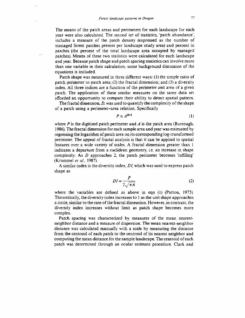
Patch shape was measured in three different ways: (1) the simple ratio of

patch perimeter to patch area; (2) the fractal dimension; and (3) a diversity

index. All three indices are a function of the perimeter and area of a given

patch. The application of these similar measures on the same data set

afforded an opportunity to compare their ability to detect spatial pattern.

The fractal dimension, D, was used to quantify the complexity of the shape

of a patch using a perimeter-area relation. Specifically

P -_ A D/z (1)

where P is the digitized patch perimeter and A is the patch area (Burrough,

1986). The fractal dimension for each sample area and year was estimated by

regressing the logarithm of patch area on its corresponding log-transformed

perimeter. The appeal of fractal analysis is that it can be applied to spatial

features over a wide variety of scales. A fractal dimension greater than 1

indicates a departure from a euclidean geometry, i.e. an increase in shape

complexity. As D approaches 2, the patch perimeter becomes 'infilling'(Krummel et aL, 1987).

A similar index is the diversity index, DI, which was used to express patch

shape as

P

Ol = 2_ (2)

where the variables are defined as above in eqn (I) (Patton, 1975).

Theoretically, the diversity index increases to 1 as the unit shape approachesa circle, similar to the case of the fractal dimension. However, in contrast, the

diversity index increases without limit as patch shape becomes morecomplex.

Patch spacing was characterized by measures of the mean nearest-

neighbor distance and a measure of dispersion. The mean nearest-neighbor

distance was calculated manually with a scale by measuring the distance

from the centroid of each patch to the centroid of its nearest neighbor and

computing the mean distance for the sample landscape. The centroid of each

patch was determined through an ocular estimate procedure. Clark and

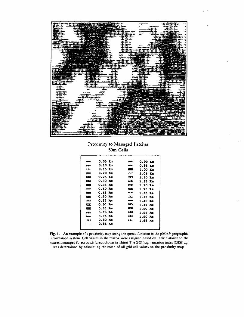
Proximity to ManagedPatches50m Cells

0.05 lr,m _ 0.9O Km,v,Jet 0.10 _ '_ 0.95 Ir_'_'. 0.15 Xm mm 1.00 It,j=

0.20 ]g.m /// 1.05 Fan0.25 _ m 1.10 lra

4mL 0.30 _ L'_'_ 1.15 ]r,mmm 0.35 Km _ 1.20 Ka

0.40 Km _ 1.25 Xml 0.4.5 Km '*°' 1.30 K"_

0.S0 ]ran _ 1.35 1_0.55 l,,m _ 1.40 Km0.60 Km Xl= 1.45 Km

na_ 0.65 _u _ 1.50 XmoH 0.70 _ _ 1.55 lr__(. 0.75 Km ur 1.60 Km_,0-. 0.80 Km ,,r** 1.65 Tan--. 0.85 Km

Fig. 1. An example of a proximity map using the spread function in the pMAP geographicinformation system. Cell values in the matrix were assigned based on their distance to the

nearest managed forest patch (areas shown in white). The GIS fragmentation index (GISfrag)

was determined by calculating the mean of all grid cell values on the proximity map.


Evans (1954) developed a measure of dispersion of patches using the equation

R = 2p1'2_ (3)

where R is dispersion, _ is the mean nearest-neighbor distance, and p is the

mean patch density (number of patches per unit area; see also Pielou, 1977,

p. 155). Dispersion is a measure of the non-randomness of the patch

arrangement. In a random population, R= 1; R less than I indicates

aggregation of the patches, while R greater than 1 indicates that the patch

population forms a regular dispersed pattern or spacing.A fifth group of statistics was calculated which predominantly reflects the

character of the matrix (in this case, natural forested land) as opposed to

managed patch configuration (clearcut areas): namely, a GIS-derived index

(christened GISfrag), matrix contiguity, interior habitat, and total patch

edge. To determine contiguity, a mylar sheet with an 8 x 8 grid consisting of

64 ceils each with a size of 27 ha was overlaid on the sample landscape maps.

The largest contiguous natural forest area (i.e. the largest number of

contiguous grid cells) in the sample landscape was recorded. Using this 8 x 8

grid, the contiguity index could potentially range from 0 (a landscape with

no natural forest patches greater than 27 ha, i.e. highly fragmented) to 64 la

landscape with no managed stands, and hence no fragmentation). A 27-ha

cell size was chosen because it was considered to be a viable habitat patchsize and fits within the structure of the existing landscape.

The GIS fragmentation index (GISfrag) was computed by first producing

a proximity map using the SPREAD function in the pMAP GIS software

(Spatial Information Systems, 1986). This procedure assigned cell values

based on the distance to the managed forest patches (i.e. a distance of one cell

away from a managed patch was equal to 50m, a distance of two cells was

equal to 100m, and so forth; see Fig. 1 for an example of a digital map

illustrating all matrix distances to managed patches). A GISfrag was

computed as the mean value of all the grid cell values on the proximity map,

including the managed patches which were assigned values of zero. Large

mean values reflected a low degree of forest fragmentation while maximumfragmentation occurred when the mean values approach zero.

The spread function in pMAP was also used to calculate the amount ofinterior forest habitat. Interior forest was defined as the amount of natural

forest remaining after removing an edge zone of 100 m (approximately two

tree heights) into the natural forest matrix (Fig. 2). The mean total edge was

simply the average of the total managed patch edges for each landscape. A

non-parametric test (Wilcoxon rank sum) for the difference between mean

values was performed for each landscape and year for each of the variables

listed above to assess the ability of these variables to reflect landscapechange.


InteriorForestHabitat

50m Ceils

S_.v-mbol Label

'.! ;":",i!'!;!:i ,'_::r': ]7:,i_',:,_!__!_'_ InteriorHabitat 57.73

Edge Effect (lOOm) 21.87

Managed Forest 20.40

Fig. 2. An example of an interior forest habitat map generated by pMAP. The interior

forest habitat is defined here as the amount of natural forest remaining after removing an

edge zone of 100m into the natural forest.


RESULTS AND DISCUSSION

Landscape structure

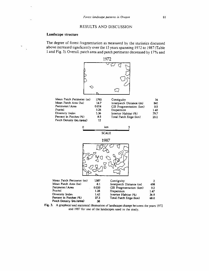
The degree of forest fragmentation as measured by the statistics discussed

above increased significantly over the 15 years spanning 1972 to 1987 (Table

1 and Fig. 3). Overall, patch area and patch perimeter decreased by 17% and

t',

Mean Patch Perimeter (m) 1793 34

Mean Patch Area (ha) 14.7 841

Perimeter/Area 0.014 0.5

Fractal 1.26 1.40

Diversity Index 1.36 79.7

Percent in Patches (%) 8.5 20.2

Patch Density (no./area) 12

1972

Nd

Contiguity

Interpatch Distance (m)

GIS Fragmentation (km)

DispersionInterior Habitat (%)

Total Patch Edge (kin)

0 km 5I I

SCALE

1987

Mean Patch Perimeter (m)

Mean Patch Area (ha)

Perimeter / AreaFractal

Diversity IndexPercent in Patches (%)

Patch Density h'mdarea)

Fig. 3.

1387 Contiguity 28.1 Interpatch Distance (m) 498

0.020 GIS Fragmentation (km) 0.21.28 Dispersion 1.471.42 Interior Habitat (%) 36.8

27.3 Total Patch Edge (km) 68.038

A graphical and statistical illustration of landscape change between the years 1972

and 1987 for one of the landscapes used in the study.

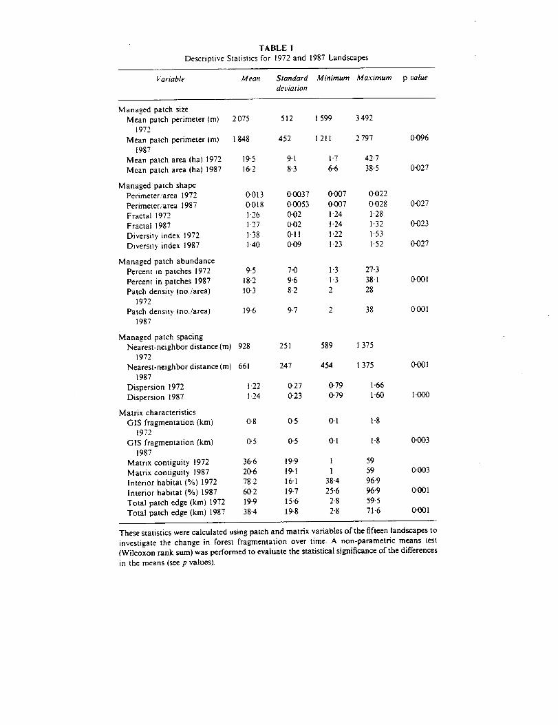
TABLE !

Descriptive Statistics for 1972 and 1987 Landscapes

Variable Mean Standard Minimum Maximum p value

deviation

Managed patch size

Mean patch perimeter (m) 2075 512

1972

Mean patch perimeter (m) 1 848 452

1987

Mean patch area {ha) 1972 19.5 9.1

Mean patch area (ha) 1987 16.2 8-3

Managed patch shape

Perimeter:area 1972 0.013

Perimeter:area 1987 00.18

Fractal 1972 1-26

Fractal 1987 1-27

Diversity index 1972 1-38

Diversity index 1987 1.40

Managed patch abundance

Percent in patches 1972 9-5 7-0

Percent in patches 1987 18.2 9'6

Patch density (no./area) 10"3 8-2

1972

Patch density (no./area) 19.6 9-7

1987

Managed patch spacing

Nearest-neighbor distance(m) 928 251

1972

Nearest-neighbor distance(m) 661 247

1987

Dispersion 1972 1"22

Dispersion 1987 1-24

Matrix characteristics

GIS fragmentation (km) 0-8 0-5

1972

GIS fragmentation (km) 0-5 0-5

1987

Matrix contiguity 1972 36-6 19-9

Matrix contiguity 1987 20-6 19-1

Interior habitat (%) 1972 78.2 16-I

Interior habitat (%) 1987 60.2 19-7

Total patch edge (kin) 1972 19-9 15-6

Total patch edge (km) 1987 38"4 19-8

I 599 3 492

1 211 2797 0.096

1.7 42.7

6-6 38.5 0.027

0-0037 0-007 0.022

0-0053 0-007 0.028 0.027

0-02 1-24 1"28

0-02 1-24 1.32 0.023

0-11 1.22 1-53

0-09 1-23 1.52 0.027

1-3 27-3

1-3 38-I

2 28

0.001

589

2 38 0-001

1 375

454 1 375 0-001

0-27 0-79 1-66

0-23 0-79 1-60 1-000

0.1 1-8

0.1 1-8 0-003

1 59

! 59 0.003

38.4 96'9

25"6 96"9 0-001

2"8 59.5

2-8 71-6 0-001

These statistics were calculated using patch and matrix variables of the fifteen landscapes to

investigate the change in forest fram'nentation over time. A non-parametric means test

(Wilcoxon rank sum) was performed to evaluate the statistical significance of the differences

in the means (see p values).


11% or from 19-5 to 16"2 ha and 2075 to 1848 m, respectively. Although some

1972 patches 'grew' by 1987 as a result of the coalescence of two or more

managed patches, individual managed patch size on the whole decreased.

The fractal dimension, the perimeter-to-area ratio, and diversity index

indicate a statistically significant increase in patch complexity over time. A

contributing factor to this increased complexity may be attributed to the

linking of several smaller managed patches which often produces an

irregularly shaped patch. The fractal dimension and diversity index appear

to be fairly robust measures of an "average' patch shape and may be capable

of discerning subtle changes in patch configuration which are difficult to

assess by visual inspection alone. In contrast, because it is not scale-

invariant, the perimeter-to-area ratio must be interpreted carefully.

Patch density increased over the 15 years by 98%. The percent of the

landscape in managed patches nearly doubled in the 15-year period from

9"5% to 18-2%. The mean of the index of contiguity decreased by 44% by

1987, reflecting the increased number of clearcuts made in the area. Not

surprisingly, the mean nearest-neighbor distance also decreased significantly

from 928 to 661 m. Dispersion, however, did not register the change in

spatial distribution of patches over time. There was no difference in

dispersion from 1972 to 1987 (1-22 versus 1"24), which represents a regular,

dispersed spacing pattern for both dates. Since dispersion is a function of

/1.8 km (36 cells) 1.4 k.,m (28 cells) 0.9 ka-n (19 ceils)

0 k.m 5

SCAI.E

0.7 km (14 ceils) 0.3 krn 16cells) 0.1 krn (2 cells)

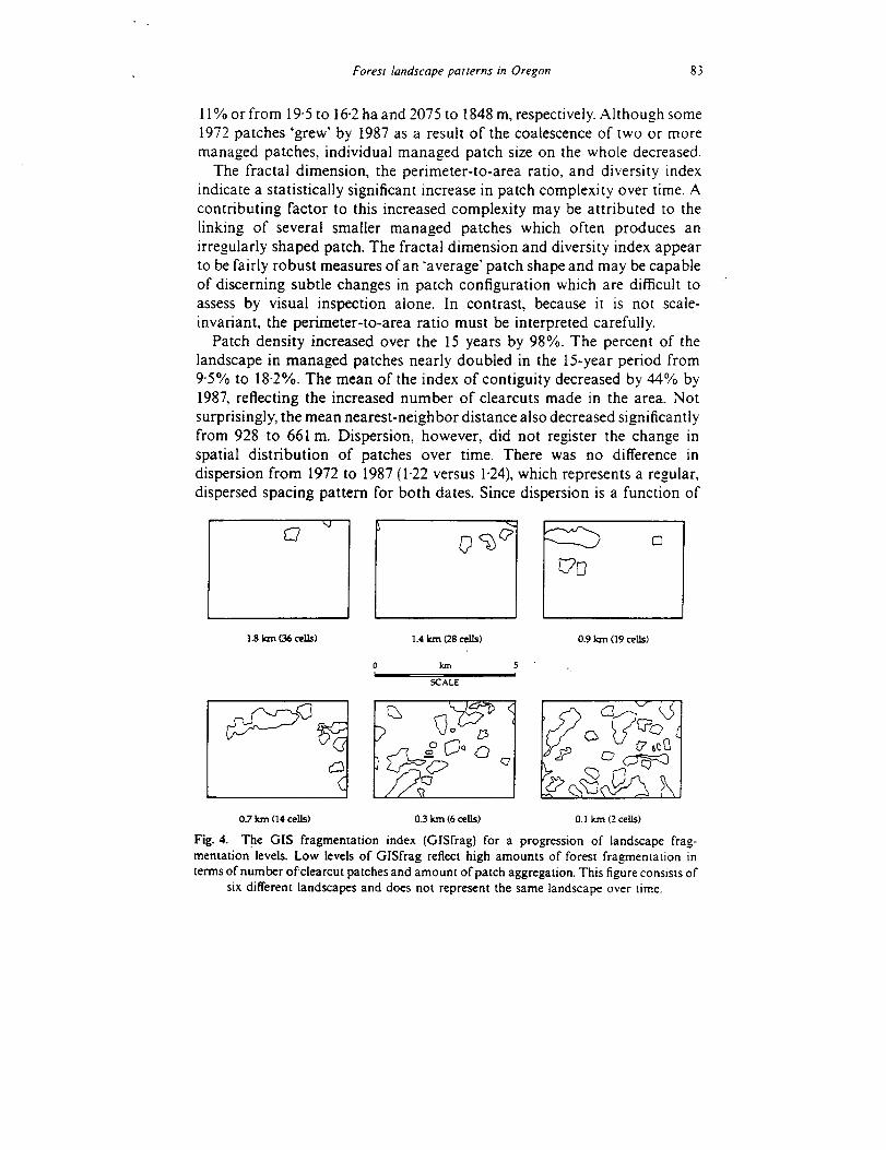
Fig. 4. The GIS fragmentation index (GISfrag) for a progression of landscape frag-

mentation levels. Low levels of GISfrag reflect high amounts of forest fram'nentation in

terms of number ofclearcut patches and amount of patch aggregation. This figure consists of

six different landscapes and does not represent the same landscape over time.

84 William J. Rtpple, G. A. Bradshaw, Thomas A. Spies

both patch density and interpatch distance, we expected it to change because

these other variables were statistically different over time. However, the

mean change in these two variables was in opposite directions, i.e. patch

density increased while nearest-neighbor distance decreased. We concludethat their combined effects canceled one another. The amount of interior

forest habitat decreased from 78-2% in 1972 to 60.2% in 1987. This decrease

in interior habitat (18% loss) was approximately twice the areal increase in

managed patches (8.7%).

The GISfrag mean decreased by 0-3 km in 1987, indicating an increase in

forest fragmentation (Table 1). Figure 4 shows the GISfrag for a progressionof landscape fragmentation levels. The GISfrag seems to be sensitive to the

abundance of patches and the amount of unfragmented contiguous natural

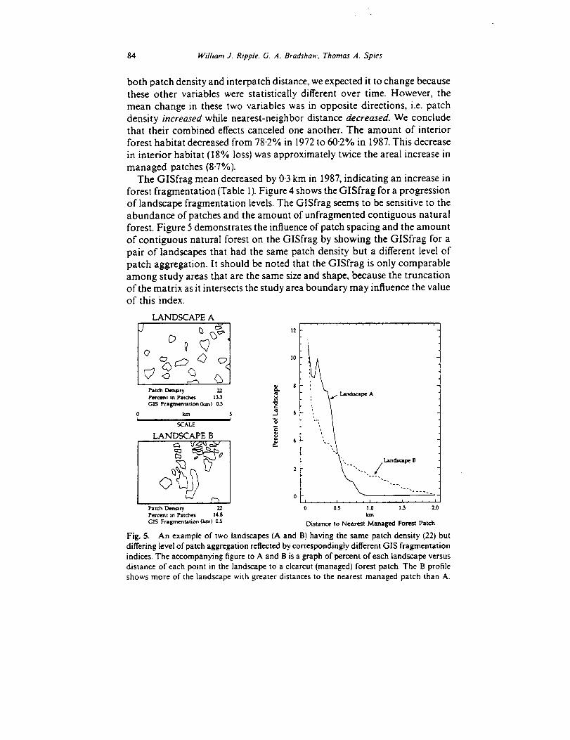
forest. Figure 5 demonstrates the influence of patch spacing and the amount

of contiguous natural forest on the GISfrag by showing the GISfrag for a

pair of landscapes that had the same patch density but a different level of

patch aggregation. It should be noted that the GISfrag is only comparable

among study areas that are the same size and shape, because the truncationof the matrix as it intersects the study area boundary may influence the valueof this index.

LANDSCAPE A

(3/Patch Density 22.

P_-'Imt in Patches 13.3

GI$ Fragmamtation(km) 03

0 kam 5I t

LANDSCAPE B

_-z_ =:_-/ I

Patch Den_ty 22

Percent in Patches 14.8

G1S Fragmentation (k.m) 0.5

scape A

I , - * * i .... i .... J .... t

0.5 1.0 1.5 2.0

kln

Distance to Nearest Managed Fort_t Patch

Fig, 5. An example of two landscapes (A and B) having the same patch density (22) but

differing level of patch aggregation reflected by correspondingly different GIS fragmentation

indices. The accompanying figure to A and B is a graph of percent of each landscape versus

distance of each point in the landscape to a clearcut (managed) forest patch. The B profile

shows more of the landscape with greater distances to the nearest managed patch than A.


Ecological and management implications

An examination of the results reveals the varying ability ofeach analysis to

describe change in patch and matrix characteristics. The nature and amount

of change detected by these different landscape statistics have significance to

the ecology and management of forest landscapes. Changes that wereevident in patch-level characteristics indicate a trend toward smaller units

and a slight trend toward more irregular units. These changes may reflect the

increased cutting on steeper, more irregular terrain, more careful "fitting' of

the cutting units as the available cutting area decreased, an effort to optimize

big game habitat by increasing the number ofcuts, and/or an effort to reduce

the visual impact of clearcutting.

The increase in the number of young, managed stand patches and the total

amount of edge has implications for habitat potential of the landscapes.Although conclusive information on the effect of edges on vertebrates in

western coniferous forest landscapes is not yet available, an increase in edge

can benefit some species but prove detrimental to others (Yahner, 1988). For

example, it has been observed that big game animals show an affinity for

edges (Brown, 1985) and that some bird species occur more frequently on

edges than in forest interiors (Rosenberg & Raphael, 1986). The fact that

edge density increased in the present study areas over the past 15 years

suggests that the habitat potential has increased for such species as elk,

which can successfully utilize the edge environment. The increased dispersal

of small clearcuts into the matrix of forest cover provides a corresponding

increase in the amount of hiding cover close to forage areas used by the elk

(Brown, 1985).

Conversely, a number of other vertebrate species, such as the northern

spotted owl, Townsend's warbler Dendroica townsendi, and pileated

woodpecker Dryocopus pileatus, may avoid edges (Bull, 1975; Brown, 1985;

Rosenberg & Raphael, 1986). The increase in edge density indicates that

habitat conditions for such species favoring interior forest have probably

declined markedly. Specifically, the decrease in the mean distance of matrixto managed patch (as measured by GISfrag) and interior forest area are

evidence of the decline in interior species habitat conditions. The manner

and degree to which the decline affects interior species populations in the

study areas are difficult to assess. Although Rosenberg and Raphael (1986)

did not find a strong response of vertebrate communities in northern

Californian landscapes which sustained a mean percent clearcut of 18%

(roughly the same as the present study), the authors warned that the

fragmentation in the region is a relatively recent phenomenon. Long-term

vertebrate responses were not yet discernible.

The continued use of dispersed clearcutting increases fragmentation of


forest landscapes at a rate more rapid than the rate ofcutting on a per areabasis. Given that the present cutting patterns are decreasing potential

interior habitat at a rapid rate, alternative cutting patterns should beconsidered to reduce the loss of interior habitat and retain the area of large

forested patches. Alternative models which aggregate cutting (Franklin &Forman, 1987) are available and may not require altering current standards

and guidelines.

CONCLUSIONS

In an attempt to describe forest fragmentation, five groups of statistics were

employed: patch abundance, patch shape, patch size, patch spacing, and

matrix characteristics. By comparing two sets of data representing two dates

over a 15-year period, we found that patch abundance, patch spacing

measures, and matrix characteristics were most useful in capturing the

amount of forest fragmentation over time. Patch size and shape statistics

contribute information on specific characteristics of the individual patches

and may be useful for applications designed to study specific interior and

edge habitats or for the prescription of new clearcuts. In addition, a GIS

fragmentation index was developed which proved sensitive to both the

quantity and spacing of patches. The GIS provides an automated method of

quantifying forest fragmentation to aid in forest and wildlife managementdecisions, and a means by which field and image data may be used in concert.

Current concerns over forest fragmentation are typically related to a

landscape condition in which forest islands occur in a matrix of managed

forest plantations. This study suggests that on many Forest Service lands inthe Cascade Range this condition is not yet realized, in contrast to many

privately owned landscapes in the Cascades in which the matrix is theharvested area and the patches are the natural forest. Consequently, in

characterizing fragmentation in some landscapes, characteristics of the

matrix (the unmanaged forest) may be of more interest than characteristics

of the patches (the managed plantations). Where the matrix is ofinterest, the

interior area, the total edge, and the mean distance to the nearest managed

patch (GISfrag) will be the useful descriptors of fragmentation. Additionalresearch is needed to document and substantiate the relationship between

forest landscape pattern and the subsequent wildlife/ecosystem response.

ACKNOWLEDGEMENTS

This project was funded in part by NASA grant number NAGW-1460. Theauthors would like to thank Robert Gaglioso for assisting in the patch


mapping and digitization, and Miles Hemstrom, E. Charles Meslow and

David H. Johnson for providing valuable suggestions on an earlier version

of the manuscript.

REFERENCES

Brown, E. R. (1985). Management of Wildlife and Fish Habitats in Forests Of WesternOregon and Washington. US Forest Service, Pacific Northwest Region,Portland, Oregon.

Bull, E. L. (1975). Habitat utilization of the pileated woodpecker, Blue Mountains,Oregon. MS thesis, Oregon State University.

Burgess, R. L. & Sharpe, D. M. (eds) (1981). Forest Island Dynamics in Man-dominated Landwapes. Springer-Ver[ag, New York.

Burrough, E A. (1986). Principles of geographic information systems for landresources assessment. Monographs on Soil and Resources Survey, No. 12.Oxford University Press, Oxford.

Clark, P. J. & Evans, E C. (1954). Distance to nearest neighbor as a measure of

spatial relationships in populations. Ecolog), 35, 445-53.Forman, R. T. T. & Godron, M. (1986). Landscape Ecology. John Wiley, Chichester.Franklin, J. E & Dyrness, C. T. (1973). Natural Vegetation of Oregon and

Washington. Oregon State University Press, Oregon.Franklin, J. E & Forman, R. T. T. (1987). Creating landscape patterns by cutting:

ecological consequences and principles. Landscape Ecol., 1, 5-18.

Harris, L. D. (1984). The Fragmented Forest. University of Chicago Press, Chicago.Krummel, J. R., Gardner, R. H., Sugihara, G., O'Neill, R. V. & Coleman, P. R. (1987).

Landscape patterns in a disturbed environment. Oikos, 48, 321-4.

Milne, B. T. (1988). Measuring the fractal geometry of landscapes. Appl. Math.Comput., 27, 67-79.

Noss, R. E (1983). A regional landscape approach to maintain diversity. BioScience,3, 7OO-6.

O'Neill, R. V., Krummel, J. R., Gardner, R. H., Sugihara, G., Jackson, B., DeAngelis,D. L., Milne, B. T., Turner, M. G., Zygmunt, B., Christensen, S. W., Dale, V. H.

& Graham, R. L. (1988). Indices of landscape pattern. Landscape Ecol., 1.153-62.

Patton, D. R. (1975). A diversity index for quantifying habitat 'edge'. Wildl. Soc.Bull., 3, 171-3.

Pielou, E. C. (1977). Mathematical Ecology. Wiley, New York.Ripple, W. J. (ed.) (1987). Geographic Information Systems for Resource

Management: A Compendium. American Society for Photogrammetry andRemote Sensing, Bethesda, Maryland.

Ripple, W. J. (ed.) (1989). Fundamentals of Geographic Information Systems: ACompendium. American Society for Photogrammetry and Remote Sensing,Bethesda, Maryland.

Ripple, W. J. & Luther, T. (1987). The Use of Digital Landsat Data for WildlifeManagement on the Warm Springs Indian Reservation of Oregon. Proc. Ann.Convention Amer. Soc. Photogramm. & Remote Sensing, Baltimore, Maryland,pp. 266--74.

Rosenberg, K. V. & Raphael, M. G. (1986). Effects of forest fragmentation on

88 William J. Rtpple, G. A. Bradshaw, Thomas A. Spies

vertebrates in Douglas-fir forests. In 14,71dlife 2000, ed. J. Verner, M.L.Morrison & C. J. Ralph. University of Wisconsin Press, Madison, Wisconsin.

pp. 263-72.Spatial Information Systems (1986). pMAP: A Software Svstern for Analysis of

Spatial Information. Omaha, Nebraska.Spies. T. A. & Franklin, J. F. (1988). Old growth and forest dynamics in the Douglas-

fir region of western Oregon and Washington. Natural Areas Joffrnal, 8,190-201.

Thomas, J. W. (ed.) (1979). Wildlife habitats in managed forests--the Blue

Mountains of Oregon and Washington. USDA For. Serv. Agric. Hdbk, No. 53.Portland, Oregon.

Yahner, R. H. (I 988). Changes in wildlife communities near edges. Conserv. Biol., 2,333-9.

Documents

USA · Range of Oregon, USA ... (Noss, 1983; Harris, 1984 ... natural forest matrix were digitally recorded as polygons for both the 1972 and 1987 data