FEDERAL RESERVE BANK OF SAN FRANCISCO

WORKING PAPER SERIES

U.S. Monetary Policy and Fluctuations of International Bank Lending

Stefan Avdjiev Bank for International Settlements

Galina Hale

Federal Reserve Bank of San Francisco

January 2018

Working Paper 2018-02

http://www.frbsf.org/economic-research/publications/working-papers/2018/02/

Suggested citation:

Avdjiev, Stefan, Galina Hale. 2018. “U.S. Monetary Policy and Fluctuations of International Bank Lending” Federal Reserve Bank of San Francisco Working Paper 2018-02. https://doi.org/10.24148/wp2018-02 The views in this paper are solely the responsibility of the authors and should not be interpreted as reflecting the views of the Federal Reserve Bank of San Francisco or the Board of Governors of the Federal Reserve System.

U.S. monetary policy and fluctuations of international bank lendingI

Stefan Avdjiev1

Bank for International Settlements

Galina Hale2

Federal Reserve Bank of San Francisco

January 11, 2018

Abstract

There is no consensus in the empirical literature on the direction in which U.S. monetary policy

affects cross-border bank lending. We find robust evidence that the impact of the U.S. federal

funds rate on cross-border bank lending in a given period depends on the prevailing international

capital flows regime and on the level of the two main components of the federal funds rate: macro

fundamentals and monetary policy stance. During episodes in which bank lending from advanced

to emerging economies is booming, the relationship between the federal funds rate and cross-

border bank lending is positive and mostly driven by the macro fundamentals component, which

is consistent with a search-for-yield behavior by internationally-active banks. In contrast, during

episodes of stagnant growth in bank lending from advanced to emerging economies, the relationship

between the federal funds rate and bank lending is negative, mainly due to the monetary policy

stance component of the federal funds rate. The latter set of results is driven by the lending to

emerging markets, which is consistent with the international bank-lending channel and flight-to-

quality behavior by internationally-active banks.

Keywords: Monetary policy spillovers, Capital flows, Bank lending

JEL codes: F21, F32, F34

IWe are grateful to Bat-el Berger, Julia Bevilaqua, and Eric Tallman for excellent research assistance. We receivedhelpful comments from Carmen Reinhart, Jonathan Ostry, Sebnem Kalemli-Ozcan, Jason Wu, and the participantsof the CUHK conference on international finance in Shenzhen, the IM-TCD-ND Workshop on International Macroe-conomics and Capital Flows in Dublin, Ireland , the Asia Pacific Policy Conference at the Federal Reserve Bank ofSan Francisco, the NES and the Moscow State University conferences in Moscow. All errors are ours. The viewspresented in this paper are solely of the authors and do not necessarily represent the views of the Federal ReserveSystem or the Bank for International Settlements.

1stefan.avdjiev@bis.org2galina.b.hale@sf.frb.org

1. Introduction

The business cycle that followed the global financial crisis demonstrated how sensitive the world

economy is to changes in U.S. monetary policy. Most countries, regardless of the exchange rate

regime, are susceptible to changes in U.S. monetary policy, unless their borders are completely

closed to international capital flows (Miranda-Agrippino and Rey, 2015). The discussion left the

purely academic domain and entered the realm of policymaking.3 Two sets of events illustrated

this quite clearly. The first one occurred in 2013, when Chairman Bernanke’s announcement of a

potential tapering of the Fed’s quantitative easing program led to sudden stops in capital flows to

emerging market economies — the episode dubbed the “taper tantrum.”4 The second set of events

took place in 2015, when a number of emerging economies raised interest rate either preemptively

or immediately following Fed’s lift–off of interest rates. Is this heightened post–crisis sensitivity to

U.S. monetary policy an anomaly, a new normal, or an old story? In this paper, we address this

question by studying the time-varying response of international bank lending to changes in U.S.

macroeconomic fundamentals and Fed’s monetary policy stance.

Our analysis differs from the large literature on U.S. monetary policy spillovers along a number

of dimensions. First, using the most comprehensive bilateral data on international bank lend-

ing available, we observe that the correlation between the federal funds rate and international

bank lending fluctuates dramatically, from highly negative to highly positive, over time.5 Using a

Markov switching regression, we identify two distinct regimes in international bank lending: (i) a

boom regime, characterized by high growth rates of lending from advanced to emerging economies

(“North–South flows”) and (ii) a stagnation regime, characterized by low or negative growth rates

of lending from advanced to emerging economies. We conduct separate sets of analyses for these

two regimes and find substantial differences between them in terms of the relationship between

international bank flows and the federal funds rate. Second, we recognize that the federal funds

rate has two distinct components — a component driven by macroeconomic fundamentals and a

component determined by the Fed’s discretionary decisions. Thus, in addition to the effects of the

federal funds rate, we analyze the effects of a Taylor rule-implied rate (the “macro fundamentals

component”) and the difference between the federal funds rate and the one implied by the Taylor

rule (the “monetary policy stance component”). Third, taking advantage of the bilateral nature of

the BIS international banking statistics, we allow for cross-border lending originating from banks

located in the U.S. to be affected differently than lending originating from outside the U.S. Fourth,

we attempt to maximize the data sample by not relying on “pull factors” — country-specific fun-

3See, for example, Powell (2013).4See Bernanke (2013) for the full text of Chairman Bernanke testimony, and Nechio (2014); Eichengreen and

Gupta (2015) for the discussion of its effects on international capital flows.5In a paper complementary to ours, Friedrich and Guerin (2016) evaluate regime switching for equity and bond

flows using EPFR data, but only going back to 2000.

2

damentals that affect capital inflows. Instead, we show that our results hold if we control for

borrower-lender fixed effects and total borrowing and total lending to each country in our sample

in each quarter.

There exists a large literature that examines the importance of global factors in driving interna-

tional capital flows in general and cross-border bank flows in particular.6 It is also well-established

that these capital flows transmit global shocks to real performance of individual economies.7 The

literature tends to distinguish global (push) factors from borrowing country-specific (pull) factors

that drive international bank lending (Spiegel, 2009; Fratzscher, 2012; Forbes and Warnock, 2012;

Burger et al., 2015).8 Two global factors have consistently emerged across empirical studies as

being important drivers: (i) global risk aversion, typically approximated by the VIX (Forbes and

Warnock, 2012; Miranda-Agrippino and Rey, 2015; Bruno and Shin, 2015b), and (ii) monetary

policy in developed countries, usually measured using policy rates in advanced economies (Milesi-

Ferretti and Tille, 2011; Shin, 2012; Rey, 2015).

The direction of the impact of global risk aversion on cross-border bank flows is generally clear:

there is abundant evidence that increases in global risk aversion lead to declines in cross-border

bank flows. Virtually all papers on the subject in the existing literature have documented that

the impact of the VIX on cross-border bank flows is negative and statistically significant.9 In our

analysis, we also find that lower risk appetite, measured by higher credit spreads or higher realized

stock market volatility, are associated with lower cross-border lending overall, and especially to

emerging markets.

In contrast to risk aversion, there is no conclusive empirical evidence regarding the direction

of the effect that advanced economies’ monetary policies have on cross-border bank flows, as doc-

umented in the survey by Koepke (2015). Several studies have found a negative and statistically

significant relationship between the two variables. For example, using data from the BIS locational

banking statistics for the 1995-2007 period, Bruno and Shin (2015a), find that U.S. interest rates

have a negative impact on cross-border bank lending. They argue that banks financing costs are

closely tied to central bank policy rates, and hence affect banks willingness to lend internationally,

including to banks in emerging economies. Ghosh et al. (2014) also use the BIS locational banking

statistics and find similar results for a larger sample of 76 advanced and emerging countries.

Several other studies, however, find the opposite, or at least mixed, results. Jeanneau and

Micu (2002) find a positive relationship between higher global interest rates and banking flows

to emerging markets, using semi-annual data from the BIS consolidated banking statistics for

6Recent papers include Fratzscher (2012); Cerutti et al. (2015); Miranda-Agrippino and Rey (2015); Byrne andFiess (2016); ?); Avdjiev et al. (2017b); Ha et al. (2017).

7See, for example, Chen and Tsang (2016); Avdjiev et al. (2017a).8For the most recent analysis of push and pull factors, see Cerutti et al. (2017b); Avdjiev et al. (2017c).9See, for example, Jeanneau and Micu (2002); Ferrucci et al. (2004); Takats (2010); Herrmann and Mihaljek

(2013); Bruno and Shin (2015a,b); Baskayay et al. (2017).

3

the 1985-2000 period. The authors argue that higher interest rates in mature economies reflect

stronger economic conditions that result in improved confidence of international lenders, which

ends up stimulating cross-border bank lending. Using micro-level U.S. banking data for the 1984-

2000 period, Goldberg (2002) obtains mixed results, with the sign of the coefficient depending on

the model specification and with different results for U.S. bank lending to Latin America compared

to emerging Asia. Cerutti et al. (2017a) also present mixed evidence for a sample of 77 (advanced

and emerging) countries. They find that cross-border bank flows are positively related to short-term

U.S. real interest rates, but are negatively affected by the U.S. term premium.

One possible explanation for the lack of conclusive empirical evidence in the above empirical

literature is that the relationship between the U.S. monetary policy and international bank lending

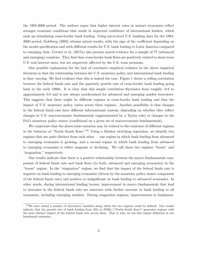
is time–varying. We find evidence that this is indeed the case. Figure 1 shows a rolling correlation

between the federal funds rate and the quarterly growth rate of cross-border bank lending going

back to the early 1980s. It is clear that this simple correlation fluctuates from roughly -0.8 to

approximately 0.8 and is not always synchronized for advanced and emerging market borrowers.

This suggests that there might be different regimes in cross-border bank lending and that the

impact of U.S. monetary policy varies across these regimes. Another possibility is that changes

in the federal funds rate have different informational content, depending on whether they reflect

changes in U.S. macroeconomic fundamentals (approximated by a Taylor rule) or changes in the

Fed’s monetary policy stance (conditional on a given set of macroeconomic fundamentals).

We conjecture that the above time-variation may be related to the existence of different regimes

in the behavior of “North–South flows.”10 Using a Markov switching regression, we identify two

regimes that are quite distinct from each other — one regime in which bank lending from advanced

to emerging economies is growing, and a second regime in which bank lending from advanced

to emerging economies is either stagnant or declining. We call these two regimes “boom” and

“stagnation,” respectively.

Our results indicate that there is a positive relationship between the macro fundamentals com-

ponent of federal funds rate and bank flows (to both, advanced and emerging economies) in the

“boom” regime. In the “stagnation” regime, we find that the impact of the federal funds rate is

negative on bank lending to emerging economies (driven by the monetary policy stance component

of the federal funds rate) and positive or insignificant on bank lending to advanced economies. In

other words, during international lending booms, improvement in macro fundamentals that lead

to increases in the federal funds rate are associate with further increase in bank lending to all

economies, including emerging markets. During stagnation regimes, improvements in fundamen-

10We have tested a number of alternative variables along which the two regimes could be defined. Our resultsindicate that the growth rate of bank lending from AEs to EMEs (“North–South flows”) generates regimes withthe most distinct impact of the federal funds rate across them. That is why, we use this regime definition in ourbenchmark estimates.

4

tals have a similar, albeit weaker effect, whereas a tightening of the monetary policy stance leads

to a decline in bank lending to emerging markets, sometimes accompanied by an increase in lend-

ing to advanced economies. Thus, the impact of macroeconomic fundamentals on cross-borer bank

lending is not regime-dependent — improvement in macro fundamentals are always associated with

higher growth in cross-border bank flows, regardless of the regime. In contrast, the impact of the

U.S. monetary policy stance on bank lending to emerging market borrowers is regime-dependent

- it is insignificant during the boom regime, but negative (and statistically significant) during the

stagnation regime.

To understand the intuition behind these results, it is useful to focus on two types of investors’

behavior. The first one, described as “return chasing,” is a high-risk-tolerance behavior charac-

terized by a propensity to allocate funds across assets primarily based on expected returns, while

paying only secondary attention to the associated risk. Classical carry trades are a good example

of such behavior. The other type of investor behavior, frequently referred to as “flight to quality,”

is a low-risk-tolerance behavior that involves moving funds into safe assets even if they offer very

low returns. During the global financial crisis, we saw a number of flight-to-quality examples. Sim-

ilarly, flight-to-quality describes well the aforementioned 2013 taper tantrum episode. If investors’

risk tolerance is time-varying, as Miranda-Agrippino and Rey (2015) has shown to be the case, we

might see time-varying response of investors to the same shock, such as a change in U.S. monetary

policy.

The story is complicated by two additional factors. First, a standard bank-lending channel of

monetary policy would also imply that an increase in cost of funds may lead to reduced risk-taking

of financial institutions and the effect of this channel can be more or less pronounced depending

on the degree of risk appetite in markets. Second, balance sheet effects create time-varying credit-

worthiness of borrowers with currency mismatches on their balance sheets depending on whether

the U.S. dollar is on the up- or down-swing, as shown by Bruno and Shin (2015a), Bruno and Shin

(2015b), Avdjiev et al. (2016), and Cesa-Bianchi et al. (2017).11

During periods of low risk tolerance or appreciating U.S. dollar, the flight-to-quality effect and

the bank lending channel are likely to dominate. During these periods, a tightening monetary

policy stance is likely to exacerbate flight-to-quality dynamics and lead to a reduction in capital

flows to emerging economies. The effect on flows to advanced economies is ambiguous and depends

on whether these countries are viewed as safe or risky and on the degree of currency mismatches

in these countries. Macroeconomic fundamentals, reflected in the Taylor rule-implied federal funds

rate, are likely to have a smaller negative effect, as improving fundamentals themselves are likely

11Of course there are other aspects of investors’ behavior that might affect their reaction to changes in U.S.monetary policy. Among those brought forth by recent literature: diversification motives, risk aversion, balance sheetcosts, portfolio composition, as well as a variety of other financial frictions. We abstract from these to keep our storytractable.

5

to increase risk tolerance.

During periods of high risk tolerance or a depreciating U.S. dollar, search-for-yield behavior is

likely to dominate. An increase in the federal funds rate, especially when driven by fundamentals,

is likely to be read by the markets as a signal of an ongoing global economic expansion. This will

improve the balance sheets of borrowers with currency mismatches, fuel market exuberance, and

intensify return-chasing, leading to increased capital flows to emerging economies despite rising cost

of funds.

One potential concern is that we use the same data to identify the regimes as the series that

are the focus of our analysis. To alleviate this concern, we construct a predicted measure of the

growth rate of bank flows from advanced to emerging economies. The explanatory variables used for

the prediction regression include global push factors as well as emerging-market-specific indicators.

The regression explains over 40 percent of the variation in the growth rate of these ”north-south”

banking flows. We then construct our regimes on the basis of these predicted flows and repeat our

analysis. We find that the results are qualitatively the same as with our benchmark analysis.

Taken together, our results paint the following picture. A higher federal funds rate tends to be

associated with higher growth of cross-border bank lending to advanced economies. This, seem-

ingly counter-intuitive, effect is driven by two factors: a) an improvement in U.S. macroeconomic

fundamentals leads to an increase in federal funds rate (via its Taylor rule component) and at the

same time increases cross-border lending worldwide; b) a tightening of the U.S. monetary policy

stance, for a given level of macro fundamentals, is associated with a re-balancing of bank lending

away from emerging markets and towards advanced economies.

The relationship between the federal funds rate and cross-border bank lending to emerging mar-

kets is regime-dependent. During booms, a higher Taylor rule-implied federal funds rate signals an

improvement in U.S. macroeconomic fundamentals, and, all else the same, better growth prospects

for emerging markets (whose growth is positively correlated with U.S. growth). This leads to in-

creases in cross-border bank lending to both AEs and EMEs. Meanwhile, the pure monetary policy

stance component of the federal funds rate only has a small effect during booms. During stagna-

tion periods, the effect of the U.S. macroeconomic fundamentals component is small. Conversely,

a higher monetary policy stance component of the federal funds rate is associated with a decline in

bank lending to emerging markets.

Despite the fact that the question we address is not new, we believe our results make an

important step towards improving our understanding of international monetary policy spillovers.

For emerging market especially, cross-border bank lending flows play a very important role in

economic fluctuations. Being able to predict their response to policy changes in the U.S. is crucial

for policymakers in these countries. Until now, making such a prediction was difficult, because of

the lack of consensus in the existing literature even on the sign of the effect. Understanding that the

impact of U.S. monetary policy on bank lending varies over time across two well–defined regimes

6

and critically depends on the drivers of the changes in the US federal funds rate, makes the above

response much more predictable. Moreover, we show evidence that supports what might seem

like contradictory or unrelated mechanisms: lending booms, cost-of-funding effects, bank-lending

channel effects, balance sheet effects, and flight-to-quality effects. All these are observed in the

data, but not at all times and not across all regions. Understanding these distinctions is crucial for

reconciling the seemingly contradicting findings of the existing literature.

The rest of this paper is organized as follows. Section 2 describes our data. Section 3 goes

over the overall trends and regime changes in the data. Section 4 presents our empirical analysis.

Section 5 concludes.

2. Data

Our data on cross-border bank lending flows is obtained from the International Banking Statis-

tics (IBS) of the Bank for International Settlements (BIS). In addition, we obtain effective federal

funds rate from FRED. 12 The Taylor rule-implied federal funds rate is obtained from Hofmann

and Bogdanova (2012). We supplement these data with broad U.S. dollar index from FRED, S&P

500 from Bloomberg, and BAA spreads from Moody’s.

Since our analysis spans almost 40 years, we do not explicitly analyze the effects of uncon-

ventional monetary policy actions, which is a more recent phenomenon.13 We do, however, use

the shadow policy rate from Wu and Xia (2016), which incorporates the effects of unconventional

monetary policy on the term structure of interest rates. We do not explicitly account for any an-

nouncement affects that were not accompanied by either a change in the federal funds rate or the

change in the shadow rate. Nevertheless, events such as the “taper tantrum” testimony are captured

in our empirical analysis via their impact on the shadow policy rate, which reflects fluctuations in

long-term interest rates.

Countries are grouped into “advanced” and “developing” according to the definitions used in

the BIS International Banking Statistics.14

We construct our bank flows series by using data from the BIS Locational Banking Statistics

by Residence (LBSR), which is the most comprehensive cross-border bank lending dataset. It

contains quarterly series from Q1 1978 to Q1 2015, which include free, restricted and confidential

observations. The data points in the latter category can only be accessed on BIS premises.

The LBSR capture the outstanding claims and liabilities of internationally active banks located

in reporting countries against counterparties residing in more than 200 countries. Banks record

their positions on an unconsolidated basis, including intragroup positions between offices of the

same banking group. The data are compiled following principles that are consistent with balance

12Publicly available at https://research.stlouisfed.org/fred2/series/FEDFUNDS.13For such analysis, see recent papers by Ammer et al. (2016); Forbes et al. (2016).14The complete lists are publicly available at http://www.bis.org/statistics/bankstats.htm.

7

of payments statistics and capture around 95 percent of all cross-border interbank business (Bank

for International Settlements, 2015).

In addition to providing a geographical breakdown of reporting banks’ cross-border claims and

liabilities, the LBSR also provide information about the currency composition and the counterparty

sector of banks’ cross-border positions. The availability of a currency breakdown in the LBSR,

coupled with the reporting of breaks in series arising from changes in methodology, reporting

practices or reporting population, enables the BIS to calculate break- and exchange rate- adjusted

changes in amounts outstanding. Such adjusted changes approximate underlying flows during a

quarter.15

On the borrowing side, we focus on a set of 114 countries, including both, Advanced Economies

(AEs) and Emerging Market Economies (EMEs).16 We use quarterly data which cover the period

from Q1 1978 to Q1 2015.

3. Overall trends and regime changes

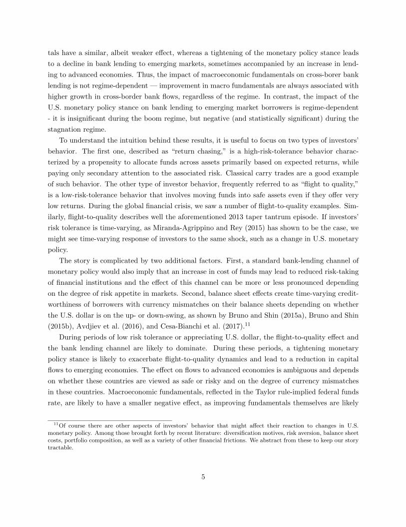
At the global level, the growth rate of cross-border bank flows varies quite a bit over time.

Figure 2 shows the quarterly growth rate of global cross-border bank claims from the LBSR. It

displays a clear cyclical pattern at low and medium frequencies. Over the past several decades,

cross-border bank lending has switched back and forth between high-growth periods and episodes

characterized by slow-downs or even outright contractions. On balance, however, we observe mostly

positive growth rates prior to 2008, reflecting a steady globalization trend.

3.1. Correlation with federal funds rate

We next turn to the analysis of the relationship between the federal funds rate and cross-border

bank flows. More specifically, we compute 12-quarter rolling correlations between the level of the

federal funds rate in quarter t and the average growth rate of several types of international bank

flows between t and t+ 7.

For the full sample of borrowers, the correlation between cross-border bank flows and the federal

funds rate exhibits a very high degree of time variation (Figure 1). It repeatedly fluctuates from

very negative values (reaching -0.8) to very positive values (reaching 0.8) over the entire time

window that we examine. Furthermore, these fluctuations do not follow a uniform pattern across

borrowing regions. Most notably, in several instances the correlation for cross-border bank flows

to EMEs deviates considerably from the respective correlation for flows to advanced economies.

15Adjusted changes may over- or underestimate underlying flows because adjusted changes may also be affected bychanges in valuations, writedowns, the underreporting of breaks, and differences between the exchange rate on thetransaction date and the quarterly average exchange rate used by the BIS to convert non-dollar amounts into USdollars.

16The complete country lists are available in Appendix A.

8

3.2. Regime changes

The cyclical pattern observed in overall cross-border flows as well as the fluctuating correlations

with federal funds rate suggest that there might be different regimes of international bank lending.

We are not the first to notice this. In a recent paper, Amiti et al. (2017) identify boom and bust

patterns in international banking and analyze demand and supply drivers of these cycles. This

cyclical pattern underscores the importance of using long time series for the analysis. The BIS

LBSR allow us to work with series that go as far back as 1978, giving us close 150 quarters of

data.17

We consider specifically changes in flows from advanced economies (AEs) to emerging market

economies (EMEs), so-called North-South flows. For these flows we observe periods of general

high growth and high volatility that are distinct from periods of either stagnation, or outright

retrenchment, and low volatility. To formally identify these regimes, we estimate a simple Markov

switching regression for quarterly growth rate of overall flows of bank lending from advanced to

emerging economies, where we allow both average level and volatility of capital flows to vary by

regime.18 For this analysis, we use the LBSR data because they provide us with the longest time

series and the cleanest growth rates, which, as discussed above, are adjusted for exchange rate

valuation effects and breaks in series. Our measure of growth rate is valuation–adjusted flows from

all advanced to all emerging economies in quarter t divided by the stock of such claims in quarter

t− 1.

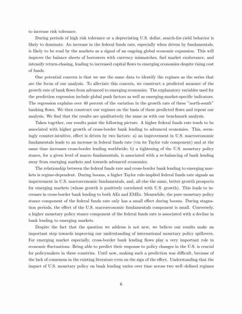
Two regimes are clearly identified. In the high-growth rate regime, the growth rate of AE

banks’ claims on EMEs is 3.4 percent on average and the volatility of the series is high. In the

complementary regime, the growth rate is negative on average (not statistically different from zero)

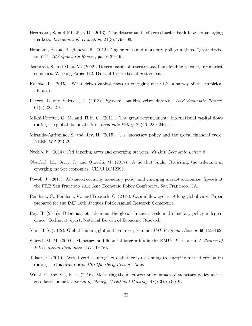
and the volatility of the series is less than half of that in the high-growth regime. Figure 3 shows

both the growth rate of aggregate lending from AEs to EMEs and the probability of the high-

growth regime. We refer to the high-growth regime as “boom” and the complementary regime

as “stagnation” and create a binary indicator of these regimes. We select a cut–off point of 50%

probability for the stagnation regime — a median probability, which results in our observations

being classified roughly equally across regimes.

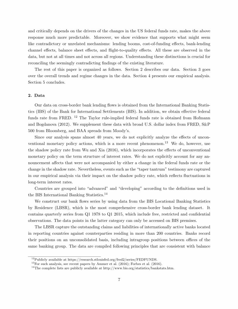
Next, we check whether regime changes are in any way connected with monetary policy cycles

in the U.S. We find that this is not the case: Figure 4 shows that there is no direct association

between the dynamics of the federal funds rate and the probability of retrenchment regime.

17As mentioned above, we use the confidential version of LBSR, which can only be accessed on the premises of theBIS.

18Estimation results are reported in Appendix Table B1.

9

3.3. Decomposing the federal funds rate

We use the Taylor rule estimates of Hofmann and Bogdanova (2012) to decompose the federal

funds rate into a business cycle component (TR) and a monetary policy stance component (MP).

More concretely, we set the business cycle component of the federal funds rate equal to the median

estimated Taylor rule-implied policy rate from Hofmann and Bogdanova (2012). We then obtain

the monetary policy stance component as the difference between the actual federal funds rate and

its business cycles component. The decomposition is displayed in Figure 5.19

We can show that this decomposition is also uncorrelated with boom/stagnation regimes in

the North-South bank lending. As shown in Table 1, the number of quarters with increases and

decreases in both TR and MP is roughly the same across regimes.

In terms of linking our results to the literature, we can think of Taylor rule-implied policy rate

as effectively capturing “good” and “bad” times as discussed in Almeida et al. (2016).

4. Empirical analysis

We split the discussion of our empirical analysis in two parts. We start by going over the

empirical setup that we use to examine the main questions in which we are interested. We then

present the key results generated by the above empirical framework and discuss the intuition behind

them.

4.1. Empirical strategy

We begin our analysis with a set of simple time-series regressions of cross-border bank lending

flows to advanced and emerging economies on the federal funds rate:

FLOWRt = α0 + α1t+ βFFt + εt, (1)

where FLOWRt is the quarterly growth rate of cross-border bank lending flows from AEs to region

R = AE,EME, and FF is the Federal Funds rate (level) in quarter t. We estimate this equation

separately for boom and stagnation regimes and include additional controls to evaluate the robust-

ness of the estimated relationships. Because we observe trends in the decomposition of the federal

funds rate, we include a trend in all regressions.

As discussed previously, we investigate the effects of two components of the Federal Funds rate

— the rate implied by the Taylor Rule, TR, and the monetary policy stance, defined as the difference

between the observed federal funds rate and the rate implied by the Taylor Rule, MP = FF −TR.

We include TR and MP together in the same regression:

FLOWRt = α0 + α1t+ β1TRt + β2MPt + εt. (2)

19Hofmann and Bogdanova (2012) calculate Taylor rule with 1.5 coefficient on inflation gap and 0.5 coefficient onoutput gap. r∗ is proxied by real trend output growth.

10

Of course, the time series regressions do not reflect important compositional changes. That is

why, we estimate panel regressions as well. Our initial approach to the panel regression analysis is

agnostic, apart from the reliance on the regimes we identified.

While we focus on a specific global push factor, the federal funds rate, we do not include

borrower-specific pull factors or lender-specific push factors. We have two reasons for doing that.

First, the (lack of) availability of reliable quarterly macroeconomic series for many borrowing

countries would necessarily limit the sample used in our analysis. Second, pull and push factors

and their effects on capital flows might vary by country or country group and might be correlated

with the federal funds rate or with capital inflows, which would potentially create bias in our

estimate of the effect of U.S. monetary policy. Instead, in our benchmark specifications, we include

the contemporaneous growth rate of total lending and total borrowing by each country in each

year to capture any lender-specific push factors and any borrower-specific pull factors. To prevent

time series fluctuations in the growth rates of total lending and total borrowing from absorbing the

effects of our global push factors, we subtract the respective quarterly averages from each of those

series.

First, we examine the overall effect of the federal funds rate by estimating the following regres-

sion:

FLOWijt = αij + α1t+ βFFt + γ1TLit + γ2TBjt + εijt, (3)

where FLOWijt is the growth rate of bank lending from country i to country j in quarter t, αij

is a set of lender-borrower country pair fixed effects. To control for country-specific push and pull

factors we also include the quarterly growth rate of total lending of country i in quarter t (TLit)

and the quarterly growth rate of total borrowing of country j in quarter t (TBjt) in deviations

from their respective quarterly means across countries.

As in the time-series regressions, we also investigate the effects of the two main components of

the Federal Funds rate — the rate implied by the Taylor Rule TR and the monetary policy stance,

defined as the difference between the observed federal funds rate and the rate implied by the Taylor

Rule MP = FF − TR. We include TR and MP simultaneously in the same regression:

FLOWijt = αij + α1t+ β1 TRt + β2 MPt + γ1TLit + γ2TBjt + εijt. (4)

We approach the heterogeneity between regimes and borrowers in two ways — we begin by

estimating separate regressions for AE and EME borrowers and for each regime Z: boom, B, and

stagnation, S. We then proceed, as a benchmark, to estimate regressions, separately for AE and

EME borrowers, where the federal funds rate, FF , or its two main components, TR and MP , are

interacted with the regime.

FLOWijt = αij + α1t+ β1 FFt ∗B + β2 FFt ∗ S + γ1TLit + γ2TBjt + εijt, (5)

FLOWijt = αij +α1t+β0Z+β1 TRt∗B+β2 TRt∗S+β3 MPt∗B+β4 MPt∗S+γ1TLit+γ2TBjt+εijt. (6)

11

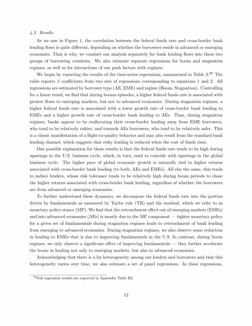
4.2. Results

As we saw in Figure 1, the correlation between the federal funds rate and cross-border bank

lending flows is quite different, depending on whether the borrowers reside in advanced or emerging

economies. That is why, we conduct our analysis separately for bank lending flows into these two

groups of borrowing countries. We also estimate separate regressions for boom and stagnation

regimes, as well as for interactions of our push factors with regimes.

We begin by reporting the results of the time-series regressions, summarized in Table 2.20 The

table reports β coefficients from two sets of regressions corresponding to equations 1 and 2. All

regressions are estimated by borrower type (AE, EME) and regime (Boom, Stagnation). Controlling

for a linear trend, we find that during booms episodes, a higher federal funds rate is associated with

greater flows to emerging markets, but not to advanced economies. During stagnation regimes, a

higher federal funds rate is associated with a lower growth rate of cross-border bank lending to

EMEs and a higher growth rate of cross-border bank lending to AEs. Thus, during stagnation

regimes, banks appear to be reallocating their cross-border lending away from EME borrowers,

who tend to be relatively riskier, and towards AEs borrowers, who tend to be relatively safer. This

is a classic manifestation of a flight-to-quality behavior and may also result from the standard bank

lending channel, which suggests that risky lending is reduced when the cost of funds rises.

One possible explanation for those results is that the federal funds rate tends to be high during

upswings in the U.S. business cycle, which, in turn, tend to coincide with upswings in the global

business cycle. The higher pace of global economic growth is naturally tied to higher returns

associated with cross-border bank lending (to both, AEs and EMEs). All else the same, this tends

to induce lenders, whose risk tolerance tends to be relatively high during boom periods to chase

the higher returns associated with cross-border bank lending, regardless of whether the borrowers

are from advanced or emerging economies.

To further understand these dynamics, we decompose the federal funds rate into the portion

driven by fundamentals as measured by Taylor rule (TR) and the residual, which we refer to as

monetary policy stance (MP). We find that the retrenchment effect out of emerging markets (EMEs)

and into advanced economies (AEs) is mostly due to the MP component — tighter monetary policy

for a given set of fundamentals during stagnation regimes leads to retrenchment of bank lending

from emerging to advanced economies. During stagnation regimes, we also observe some reduction

in lending to EMEs that is due to improving fundamentals in the U.S. In contrast, during boom

regimes, we only observe a significant effect of improving fundamentals — they further accelerate

the boom in lending not only to emerging markets, but also to advanced economies.

Acknowledging that there is a lot heterogeneity among our lenders and borrowers and that this

heterogeneity varies over time, we also estimate a set of panel regressions. In these regressions,

20Full regression results are reported in Appendix Table B2.

12

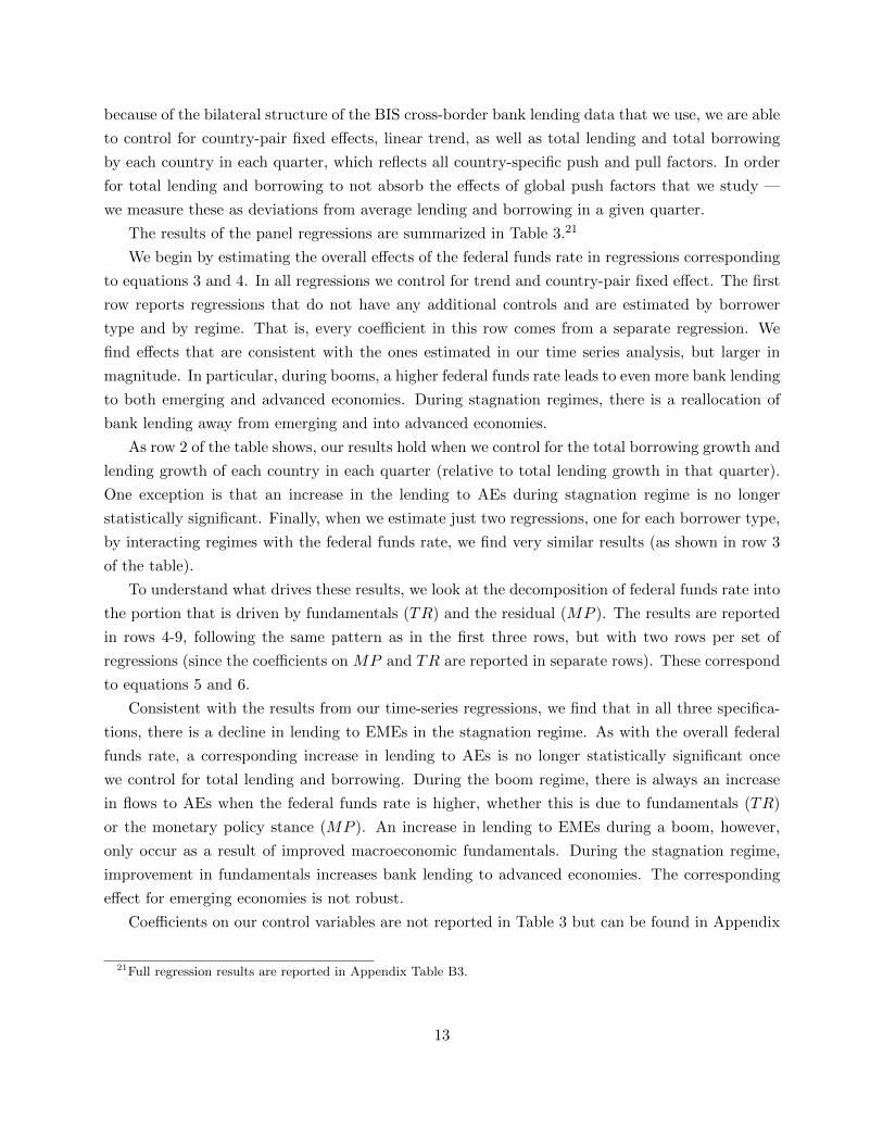
because of the bilateral structure of the BIS cross-border bank lending data that we use, we are able

to control for country-pair fixed effects, linear trend, as well as total lending and total borrowing

by each country in each quarter, which reflects all country-specific push and pull factors. In order

for total lending and borrowing to not absorb the effects of global push factors that we study —

we measure these as deviations from average lending and borrowing in a given quarter.

The results of the panel regressions are summarized in Table 3.21

We begin by estimating the overall effects of the federal funds rate in regressions corresponding

to equations 3 and 4. In all regressions we control for trend and country-pair fixed effect. The first

row reports regressions that do not have any additional controls and are estimated by borrower

type and by regime. That is, every coefficient in this row comes from a separate regression. We

find effects that are consistent with the ones estimated in our time series analysis, but larger in

magnitude. In particular, during booms, a higher federal funds rate leads to even more bank lending

to both emerging and advanced economies. During stagnation regimes, there is a reallocation of

bank lending away from emerging and into advanced economies.

As row 2 of the table shows, our results hold when we control for the total borrowing growth and

lending growth of each country in each quarter (relative to total lending growth in that quarter).

One exception is that an increase in the lending to AEs during stagnation regime is no longer

statistically significant. Finally, when we estimate just two regressions, one for each borrower type,

by interacting regimes with the federal funds rate, we find very similar results (as shown in row 3

of the table).

To understand what drives these results, we look at the decomposition of federal funds rate into

the portion that is driven by fundamentals (TR) and the residual (MP ). The results are reported

in rows 4-9, following the same pattern as in the first three rows, but with two rows per set of

regressions (since the coefficients on MP and TR are reported in separate rows). These correspond

to equations 5 and 6.

Consistent with the results from our time-series regressions, we find that in all three specifica-

tions, there is a decline in lending to EMEs in the stagnation regime. As with the overall federal

funds rate, a corresponding increase in lending to AEs is no longer statistically significant once

we control for total lending and borrowing. During the boom regime, there is always an increase

in flows to AEs when the federal funds rate is higher, whether this is due to fundamentals (TR)

or the monetary policy stance (MP ). An increase in lending to EMEs during a boom, however,

only occur as a result of improved macroeconomic fundamentals. During the stagnation regime,

improvement in fundamentals increases bank lending to advanced economies. The corresponding

effect for emerging economies is not robust.

Coefficients on our control variables are not reported in Table 3 but can be found in Appendix

21Full regression results are reported in Appendix Table B3.

13

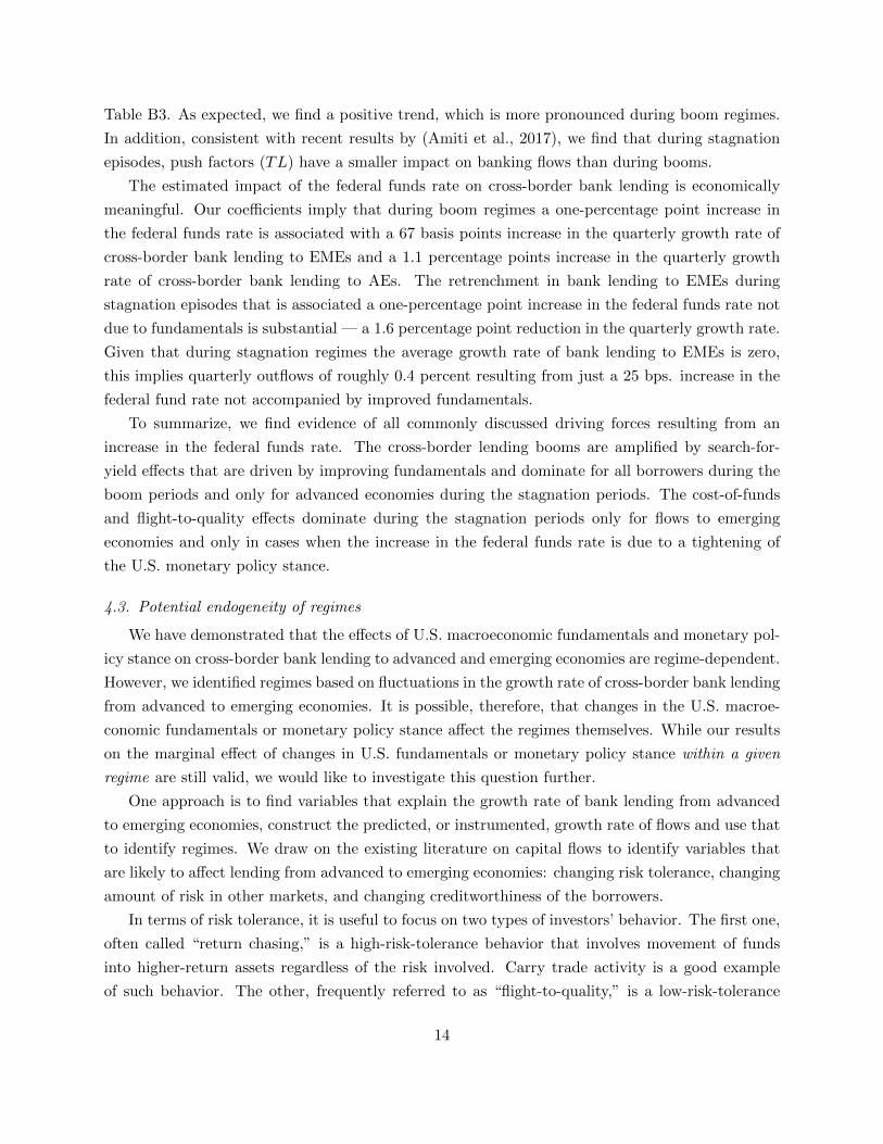
Table B3. As expected, we find a positive trend, which is more pronounced during boom regimes.

In addition, consistent with recent results by (Amiti et al., 2017), we find that during stagnation

episodes, push factors (TL) have a smaller impact on banking flows than during booms.

The estimated impact of the federal funds rate on cross-border bank lending is economically

meaningful. Our coefficients imply that during boom regimes a one-percentage point increase in

the federal funds rate is associated with a 67 basis points increase in the quarterly growth rate of

cross-border bank lending to EMEs and a 1.1 percentage points increase in the quarterly growth

rate of cross-border bank lending to AEs. The retrenchment in bank lending to EMEs during

stagnation episodes that is associated a one-percentage point increase in the federal funds rate not

due to fundamentals is substantial — a 1.6 percentage point reduction in the quarterly growth rate.

Given that during stagnation regimes the average growth rate of bank lending to EMEs is zero,

this implies quarterly outflows of roughly 0.4 percent resulting from just a 25 bps. increase in the

federal fund rate not accompanied by improved fundamentals.

To summarize, we find evidence of all commonly discussed driving forces resulting from an

increase in the federal funds rate. The cross-border lending booms are amplified by search-for-

yield effects that are driven by improving fundamentals and dominate for all borrowers during the

boom periods and only for advanced economies during the stagnation periods. The cost-of-funds

and flight-to-quality effects dominate during the stagnation periods only for flows to emerging

economies and only in cases when the increase in the federal funds rate is due to a tightening of

the U.S. monetary policy stance.

4.3. Potential endogeneity of regimes

We have demonstrated that the effects of U.S. macroeconomic fundamentals and monetary pol-

icy stance on cross-border bank lending to advanced and emerging economies are regime-dependent.

However, we identified regimes based on fluctuations in the growth rate of cross-border bank lending

from advanced to emerging economies. It is possible, therefore, that changes in the U.S. macroe-

conomic fundamentals or monetary policy stance affect the regimes themselves. While our results

on the marginal effect of changes in U.S. fundamentals or monetary policy stance within a given

regime are still valid, we would like to investigate this question further.

One approach is to find variables that explain the growth rate of bank lending from advanced

to emerging economies, construct the predicted, or instrumented, growth rate of flows and use that

to identify regimes. We draw on the existing literature on capital flows to identify variables that

are likely to affect lending from advanced to emerging economies: changing risk tolerance, changing

amount of risk in other markets, and changing creditworthiness of the borrowers.

In terms of risk tolerance, it is useful to focus on two types of investors’ behavior. The first one,

often called “return chasing,” is a high-risk-tolerance behavior that involves movement of funds

into higher-return assets regardless of the risk involved. Carry trade activity is a good example

of such behavior. The other, frequently referred to as “flight-to-quality,” is a low-risk-tolerance

14

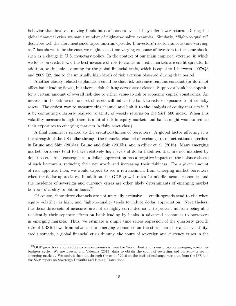
behavior that involves moving funds into safe assets even if they offer lower return. During the

global financial crisis we saw a number of flight-to-quality examples. Similarly, “flight-to-quality”

describes well the aforementioned taper tantrum episode. If investors’ risk tolerance is time-varying,

as ? has shown to be the case, we might see a time-varying response of investors to the same shock,

such as a change in U.S. monetary policy. In the context of our main empirical exercise, in which

we focus on credit flows, the best measure of risk tolerance in credit markets are credit spreads. In

addition, we include a dummy for the global financial crisis, which is equal to 1 between 2007:Q3

and 2009:Q2, due to the unusually high levels of risk aversion observed during that period.

Another closely related explanation could be that risk tolerance remains constant (or does not

affect bank lending flows), but there is risk-shifting across asset classes. Suppose a bank has appetite

for a certain amount of overall risk due to either value-at-risk or economic capital constraints. An

increase in the riskiness of one set of assets will induce the bank to reduce exposures to other risky

assets. The easiest way to measure this channel and link it to the analysis of equity markets in ?

is by computing quarterly realized volatility of weekly returns on the S&P 500 index. When this

volatility measure is high, there is a lot of risk in equity markets and banks might want to reduce

their exposures to emerging markets (a risky asset class).

A final channel is related to the creditworthiness of borrowers. A global factor affecting it is

the strength of the US dollar through the financial channel of exchange rate fluctuations described

in Bruno and Shin (2015a), Bruno and Shin (2015b), and Avdjiev et al. (2016). Many emerging

market borrowers tend to have relatively high levels of dollar liabilities that are not matched by

dollar assets. As a consequence, a dollar appreciation has a negative impact on the balance sheets

of such borrowers, reducing their net worth and increasing their riskiness. For a given amount

of risk appetite, then, we would expect to see a retrenchment from emerging market borrowers

when the dollar appreciates. In addition, the GDP growth rates for middle income economies and

the incidence of sovereign and currency crises are other likely determinants of emerging market

borrowers’ ability to obtain loans.22

Of course, these three channels are not mutually exclusive — credit spreads tend to rise when

equity volatility is high, and flight-to-quality tends to induce dollar appreciation. Nevertheless,

the these three sets of measures are not so highly correlated so as to prevent us from being able

to identify their separate effects on bank lending by banks in advanced economies to borrowers

in emerging markets. Thus, we estimate a simple time series regression of the quarterly growth

rate of LBSR flows from advanced to emerging economies on the stock market realized volatility,

credit spreads, a global financial crisis dummy, the count of sovereign and currency crises in the

22GDP growth rate for middle income economies is from the World Bank and is our proxy for emerging economiesbusiness cycle. We use Laeven and Valencia (2013) data to obtain the count of sovereign and currency crises inemerging markets. We update the data through the end of 2016 on the basis of exchange rate data from the IFS andthe S&P report on Sovereign Defaults and Rating Transitions.

15

emerging markets, the median EME GDP growth rate, and the quarterly change in the broad U.S.

dollar index. The results are reported in Table 4. We can see that all three channels are present:

all variables have statistically significant effects on the bank lending from advanced to emerging

economies.

Using the results of this regression, we construct the predicted growth rate of bank lending from

advanced to emerging economies and subject it to the same Markov switching regression analysis

as we did with raw data. Again, we identify two distinct regimes: the high-growth rate regime,

which has an average growth rate of AE banks’ claims on EMEs of 2.7 percent and high volatility;

and the complementary regime, which has an average growth rate of 1.2 percent and volatility that

is less than half of that in the high-growth regime. We refer to the above high-growth regime as

“predicted boom” and the above complementary regime as “predicted stagnation” and create a

binary indicator of these regimes. As before, we select a cut–off point of 50% probability for the

predicted stagnation regime — a median probability, which results in our observations being split

roughly equally across regimes.

Finally, we repeat our benchmark regression analysis using these predicted regimes and the

same specification as in rows 8 and 9 of Table 3. The results are summarized in the Table 5 with

full regressions reported in Appendix Table B4. We find the same pattern as in our benchmark

analysis — during both regimes, improvements in U.S. fundamentals are associated with increases

in all cross-border bank lending, more so in booms than in stagnation periods. The impact of a

tightening in the U.S. monetary policy stance, varies considerably across regimes. During booms,

it is associated with higher bank lending to both AEs and EMEs. By contrast, during stagnation,

it redirects bank lending flows away from emerging and towards advanced economies.

4.4. Robustness tests

We subject all our benchmark regressions to a variety of robustness tests and decompositions.

Here we emphasize just the most important ones.

Even though we control for country-pair fixed effects, country-specific total lending and borrow-

ing, as well as for a time trend, our main specifications do not include bilateral control variables.

In a recent paper, Obstfeld et al. (2017) show that exchange rate flexibility affects the response of

banking flows to global financial conditions. To account for this as well as for potential carry trade

flows, we include as a control variable changes in the bilateral exchange rate between the currencies

of the lending and borrowing countries or between the currencies of the borrowing countries and

the U.S. Dollar. In rows 1-4 of Table 6, we show the results of benchmark regression defined by

equation 6, where we add controls for quarterly changes in the (lender-borrower) bilateral exchange

rate or in the bilateral exchange rate of the borrowing country’s currency vis-a-vis the U.S. dollar.23

23Full regressions are reported in Appendix Table B5.

16

We find that our main effects remain essentially unchanged. The coefficients on the (lender-

borrower) bilateral exchange rate changes are never significant, while the coefficient on the change

of the exchange rate vs. U.S. dollar is negative and statistically significant for lending to advanced

economies. The latter result implies that a depreciation of the borrowing country’s currency versus

the U.S. dollar is associated with a decline in cross-border lending to that country (in line with the

predictions of Bruno and Shin (2015a)).

Next we test whether there is a lagged response of bank lending to changes in monetary policy.

To do so, we lag both MP and TR by one quarter and re-estimate our benchmark regression,

interacting these lagged values with dummies for boom and expansion regimes. The results are

reported in rows 5 and 6 of Table 6. We find that the main results are essentially unchanged. The

only exception is that now we find a statistically significant (albeit small) decline in lending to

EMEs during boom episodes as a result of an increase in MP. This is consistent with our discussion

— since the increase in MP increases the cost of funds without a simultaneous improvement in

fundamentals, it is reasonable to expect some retrenchment from risky assets even during boom

episodes.

The data allows us to split our sample into lending to banks and lending to non-banks. We

take advantage of this to test whether our results are driven by borrowers in a specific sector. As

we observed in Figure 2, cross-border interbank lending is much more volatile than cross-border

lending to non-banks. Even though the two series have grown at roughly the same average quarterly

pace since 1978 (2.3 percent for claims on non-banks and 2.1 percent for interbank claims), the

standard deviation of the cross-border interbank lending (3.2%) is nearly 50 percent higher than

that of cross-border lending to non-banks (2.2%). Thus, we might expect that the sensitivity of

cross-border bank lending to changes in the federal funds rate is higher for lending to banks than

to non-banks.

The results are reported in rows 7-10 of Table 6. We find that for most part there is no

substantial difference between lending to banks and non-banks — in both cases we observe the

same pattern as in our benchmark regressions. Nevertheless, that set of results does reveal that the

insignificant impact of MP on lending to (all sectors in) EMEs during boom regimes is the outcome

of its offsetting (statistically significant) impacts on lending to banks (negative) and lending to

non-banks (positive). Thus, it appears that lending to banks is more sensitive to fluctuations in

the cost of funds, while lending to non-banks is affected more by search-for-yield dynamics.

While we control for individual countries’ total borrowing and lending and for global push

factors, it is possible that borrowing is also affected by factors common to emerging economies. In

particular, since we find a sharp distinction between EMEs and AEs when it comes to the estimated

responses of bank lending to push factors in the stagnation period, we would like to test whether

these might be due to business cycle or crisis cycle dynamics in the emerging economies. That is

why we include controls for GDP growth rates in middle income economies, commodity indices, as

17

well as for the count of sovereign and currency crises in EME economies.24

The results are reported in rows 11-12 of Table 6. We find that our main story remains the same.

The only substantial difference relative to the benchmark results is that now we find a negative

effect of a tighter monetary policy stance on bank lending to EMEs during boom periods. That

said, this negative effect is five times smaller than in the stagnation period and is only borderline

statistically significant.

In the interest of space we don’t present all other robustness tests, but we enumerate them

briefly here.

1. The dynamics of lending to advanced economies is not driven by “safe haven” countries. When

we isolate safe havens from AEs, we find that there is no difference in the regression results

for AEs that are commonly viewed as safe havens and the remaining AEs in our sample.25

2. Our results are driven by banks’ loans and deposits rather than by banks’ holdings of debt

securities. Since our data cover exclusively lending by banks, only a small portion of overall

bond flows are captured by our empirical analysis. As a consequence, we cannot say much

about the response of portfolio debt flows to changes in the federal funds rate.

3. Our results are robust to excluding the Global Financial Crisis period: 2007:Q3 through

2009:Q2. Our results are also robust to excluding the Volker era: 1979-1992.

4. Our key results are also robust to allowing for three (rather than two) regimes. In an alter-

native set of estimations, we identify three regimes in cross-border bank lending: (i) normal

regime, (ii) boom regime, and (iii) bust regime. The estimated impacts of U.S. macroeco-

nomic fundamentals and the U.S. monetary policy stance in the three-state boom regime are

the same as in the two-state boom regime. The effects of these variables are not statistically

different from each other for the (three-state) bust and normal regimes and are the same as

in the two-state stagnation regime.

5. Controlling for the duration of the regime (the number of quarters since the last regime

change) does not alter our results.

6. Our results remain essentially unchanged if we include borrower- and lender-specific trends.

7. Our main results also remain intact if we include interactions of TR and MP with credit

spreads, realized volatility, and dollar appreciation.

5. Conclusion

In this paper, we take a new approach to the old question on the impact of U.S. monetary policy

on cross-border bank lending in order to reconcile the contradictory findings of the existing empirical

24Reinhart et al. (2017) show that capital flow cycles interact with commodity price cycle and both are related tosovereign defaults and other financial crises.

25We define the following countries as safe havens: United States, Germany, Switzerland, Japan, United Kingdomand the Netherlands.

18

literature on the topic. More concretely, we present robust evidence that the relationship between

the federal funds rate and cross-border bank lending is time-varying and depends on whether the

main drivers of fluctuations in the federal funds rate are related to changes in U.S. macroeconomic

fundamentals or to changes in the U.S. monetary policy stance.

In order to arrive to the above conclusions, we depart from the existing literature along two

key dimensions. First, we use a Markov switching regression to identify two distinct regimes in

international bank lending: (i) a boom regime, characterized by high growth rates and high volatility

of lending from AEs to EMEs and (ii) a stagnation regime, characterized by low or negative growth

rates and low volatility of lending from AEs to EMEs. Second, we decompose the federal funds rate

into two distinct components — a macroeconomic fundamentals component (approximated by the

Taylor rule-implied federal funds rate) and a monetary policy stance component (approximated by

the difference between actual federal funds rate and its Taylor rule-implied counterpart).

Our results indicate that during booms, the relationship between the federal funds rate and

cross-border bank lending is positive and mostly driven by the macro fundamentals component of

the federal funds rate. This set of results is indicative of a search-for-yield behavior on the part

of internationally-active banks. Conversely, during stagnation regimes, the relationship between

the federal funds rate and bank lending is negative and mainly due to the monetary policy stance

component of the federal funds rate. The latter set of results is most pronounced for lending to

emerging markets, which is consistent with the international bank-lending channel and flight-to-

quality behavior by internationally-active banks. These results hold if we repeat the analysis on

the basis of instrumented growth rate of bank lending from advanced to emerging economies.

These findings help us understand the considerable time variation in the raw correlation between

the federal funds rate and the growth rate of banking claims presented in Figure 1. We tend to

observe positive correlation between the federal funds rate and the growth rate of banking flows

to both advanced and emerging economies during boom episodes. In contrast, during stagnation

periods, the federal funds rate has a negative correlation with bank flows to emerging markets, but

a positive correlation with bank flows to advanced economies. This is exactly what we find in our

regression analysis.

The significance of our findings extends along several dimensions. First, they improve our

overall understanding of the effects of U.S. monetary policy on cross-border bank flows. Second,

they point to the reasons other studies in the existing empirical literature on the topic may have

found conflicting results. Third, our results help place in a coherent conceptual framework seemingly

contradictory or unrelated mechanisms, such as lending booms, cost-of-funding effects, bank-lending

channel effects, balance sheet effects, and flight-to-quality effects. Last but not least, our analysis

has important policy implications. Namely, it suggests that conditioning on the two regimes we

uncover and on the two main components of the federal funds rate could make the impact of U.S.

monetary policy on cross-border bank lending flows to any country or region much more predictable.

19

Bibliography

Almeida, M., Straub, R., and Van Robays, I. (2016). U.s. monetary policy spillovers: Good versus

bad times. Mimeo.

Amiti, M., McGuire, P. M., and Weinstein, D. E. (2017). Supply- and demand-side factors in global

banking. CEPR Discussion Paper 12091.

Ammer, J., De Pooter, M., Erceg, C. J., and Kamin, S. (2016). International spillovers of monetary

policy. Board of Governors of the Federal Reserve System IFDP Notes.

Avdjiev, S., Bruno, V., Koch, C., and Shin, H. S. (2017a). The dollar exchange rate as a global

risk factor: evidence from investment. Paper prepared for the IMF 18th Jacques Polak Annual

Research Conference.

Avdjiev, S., Du, W., Koch, C., and Shin, H. S. (2016). The dollar, bank leverage and deviations

from covered interest parity. BIS Working Paper 582.

Avdjiev, S., Gambacorta, L., Goldverg, L., and Schiaffi, S. (2017b). The shifting drivers of global

liquidity. BIS WP No 644.

Avdjiev, S., Hardy, B., Kalemli-Ozcan, S., and Serven, L. (2017c). Gross capital flows by banks,

corporates and sovereigns. NBER Working Papers, no 23116.

Bank for International Settlements (2015). Introduction to bis statistics. BIS Quarterly Review.

Baskayay, Y. S., di Giovanni, J., Kalemli-Ozcan, S., and Ulu, M. F. (2017). International spillovers

and local credit cycles. NBER WP 23149.

Bernanke, B. (2013). The economic outlook. Testimony before the Joint Economic Committee,

U.S. Congress, Washington, DC, May 22.

Bruno, V. and Shin, H. S. (2015a). Capital Flows and the Risk-Taking Channel of Monetary Policy.

Journal of Monetary Economics, 71:119–132.

Bruno, V. and Shin, H. S. (2015b). Cross-Border Banking and Global Liquidity. The Review of

Economic Studies, 82(2):535–564.

Burger, J. D., Sengupta, R., Warnock, F. E., and Warnock, V. C. (2015). U.S. Investment in Global

Bond Markets: As the Fed Pushes, Some EMEs Pull. Economic Policy, 30(84):729–766.

Byrne, J. P. and Fiess, N. (2016). International capital flows to emerging markets: national and

global determinants. Journal of International Money and Finance, 61:82–100.

20

Cerutti, E., Claessens, S., and Ratnovski, L. (2017a). Global liquidity and drivers of cross-border

bank flows. Economic Policy, 32(89):81–125.

Cerutti, E., Claessens, S., and Rose, A. K. (2017b). How important is the global financial cycle?

evidence from capital flows. BIS Working Paper 661.

Cerutti, E., Hale, G., and Minoiu, C. (2015). Financial crises and the composition of cross-border

lending. Journal of International Money and Finance, 52:60–81.

Cesa-Bianchi, A., Ferrero, A., and Rebucci, A. (2017). International credit supply shocks. NBER

WP 23841.

Chen, H. and Tsang, A. (2016). The impact of us monetary policy and other external shocks on

the hong kong economy: A factor-augmented var approach.

Eichengreen, B. and Gupta, P. (2015). Tapering talk: The impact of expectations of reduced federal

reserve security purchases on emerging markets. Emerging Markets Review, 25:1–15.

Ferrucci, G., Herzberg, V., Soussa, F., and Taylor, A. (2004). Understanding capital flows to

emerging market economies. Financial Stability Review, 16:89–97.

Forbes, K., Reinhardt, D., and Wieladek, T. (2016). The spillovers, interactions, and (un) intended

consequences of monetary and regulatory policies. National Bureau of Economic Research Work-

ing Paper w22307.

Forbes, K. J. and Warnock, F. E. (2012). Capital flow waves: Surges, stops, flight, and retrench-

ment. Journal of International Economics, 88(2):235–251.

Fratzscher, M. (2012). Capital flows, push versus pull factors and the global financial crisis. Journal

of International Economics, 88(2):341–356.

Friedrich, C. and Guerin, P. (2016). The dynamics of capital flow episodes. Bank of Canada Staff

Working Paper 2016-9.

Ghosh, A. R., Qureshi, M. S., Kim, J. I., and Zalduendo, J. (2014). Surges. Journal of International

Economics, 92(2):266–285.

Goldberg, L. (2002). When Is U.S. Bank Lending to Emerging Markets Volatile? In Frankel, J.

and Edwards, S., editors, Preventing Currency Crises in Emerging Markets. National Bureau of

Economic Research.

Ha, J., Kose, A., Otrok, C., and Prasad, E. (2017). Global macro-financial cycles and spillovers.

Paper prepared for the IMF 18th Jacques Polak Annual Research Conference.

21

Herrmann, S. and Mihaljek, D. (2013). The determinants of cross-border bank flows to emerging

markets. Economics of Transition, 21(3):479–508.

Hofmann, B. and Bogdanova, B. (2012). Taylor rules and monetary policy: a global ”great devia-

tion”?”. BIS Quarterly Review, pages 37–49.

Jeanneau, S. and Micu, M. (2002). Determinants of international bank lending to emerging market

countries. Working Paper 112, Bank of International Settlements.

Koepke, R. (2015). What drives capital flows to emerging markets? a survey of the empirical

literature.

Laeven, L. and Valencia, F. (2013). Systemic banking crises databse. IMF Economic Review,

61(2):225–270.

Milesi-Ferretti, G. M. and Tille, C. (2011). The great retrenchment: International capital flows

during the global financial crisis. Economic Policy, 26(66):289–346.

Miranda-Agrippino, S. and Rey, H. (2015). U.s. monetary policy and the global financial cycle.

NBER WP 21722.

Nechio, F. (2014). Fed tapering news and emerging markets. FRBSF Economic Letter, 6.

Obstfeld, M., Ostry, J., and Qureshi, M. (2017). A tie that binds: Revisiting the trilemma in

emerging market economies. CEPR DP12093.

Powell, J. (2013). Advanced economy monetary policy and emerging market economies. Speech at

the FRB San Francisco 2013 Asia Economic Policy Conference, San Francisco, CA.

Reinhart, C., Reinhart, V., and Trebesch, C. (2017). Capital flow cycles: A long global view. Paper

prepared for the IMF 18th Jacques Polak Annual Research Conference.

Rey, H. (2015). Dilemma not trilemma: the global financial cycle and monetary policy indepen-

dence. Technical report, National Bureau of Economic Research.

Shin, H. S. (2012). Global banking glut and loan risk premium. IMF Economic Review, 60:155–192.

Spiegel, M. M. (2009). Monetary and financial integration in the EMU: Push or pull? Review of

International Economics, 17:751–776.

Takats, E. (2010). Was it credit supply? cross-border bank lending to emerging market economies

during the financial crisis. BIS Quarterly Review, June.

Wu, J. C. and Xia, F. D. (2016). Measuring the macroeconomic impact of monetary policy at the

zero lower bound. Journal of Money, Credit and Banking, 48(2-3):253–291.

22

Figure 1: Rolling correlation between federal funds rate and quarterly growth rate of LBSR claims.

Figure 2: Quarterly growth rate of LBSR claims.

23

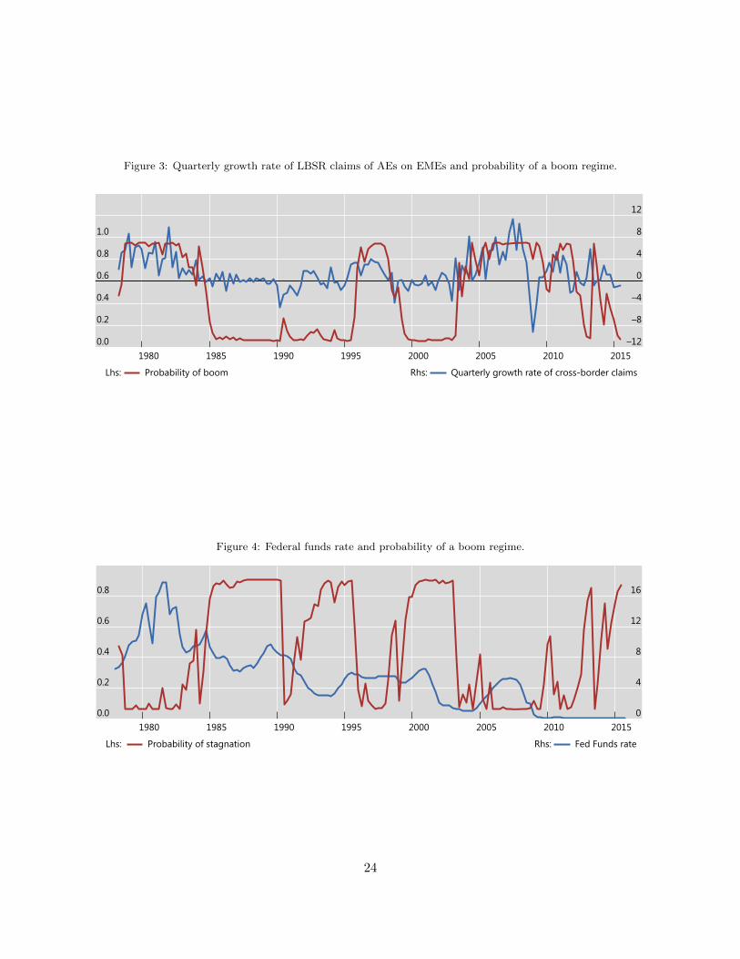
Figure 3: Quarterly growth rate of LBSR claims of AEs on EMEs and probability of a boom regime.

1.0

0.8

0.6

0.4

0.2

0.0

12

8

4

0

–4

–8

–1220152010200520001995199019851980

Probability of boomLhs: Quarterly growth rate of cross-border claimsRhs:

Figure 4: Federal funds rate and probability of a boom regime.

0.8

0.6

0.4

0.2

0.0

16

12

8

4

020152010200520001995199019851980

Fed Funds rateRhs:Probability of stagnationLhs:

24

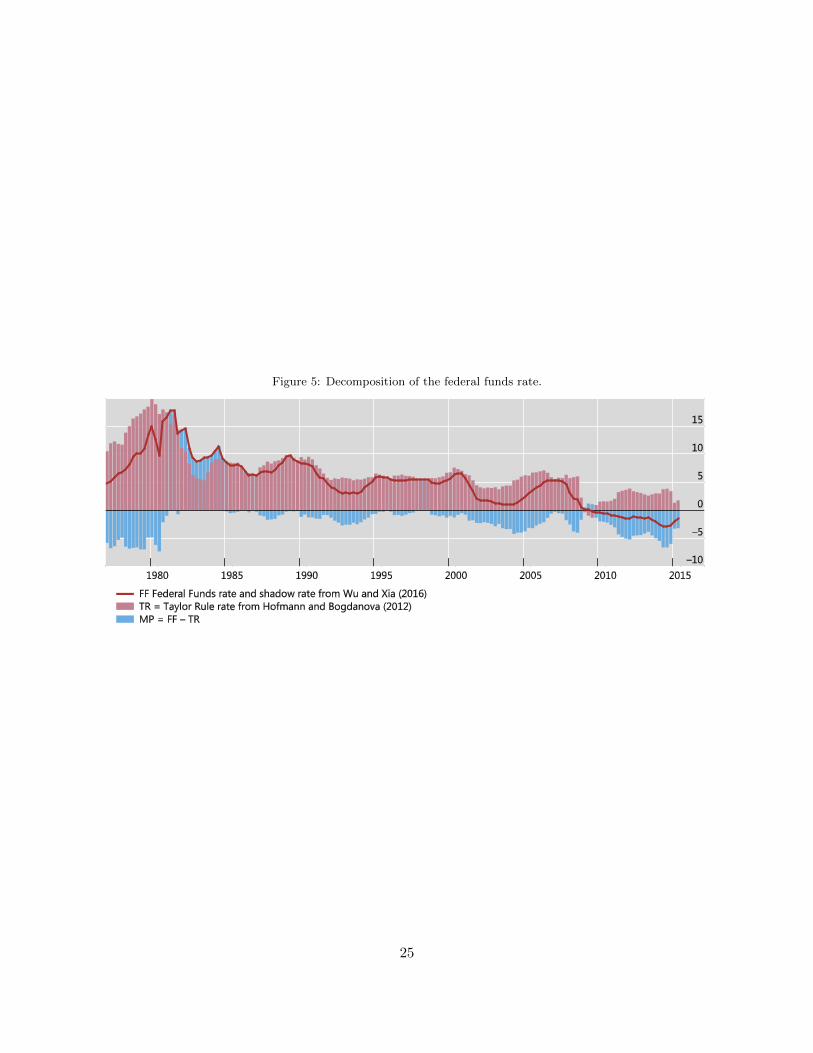
Figure 5: Decomposition of the federal funds rate.

25

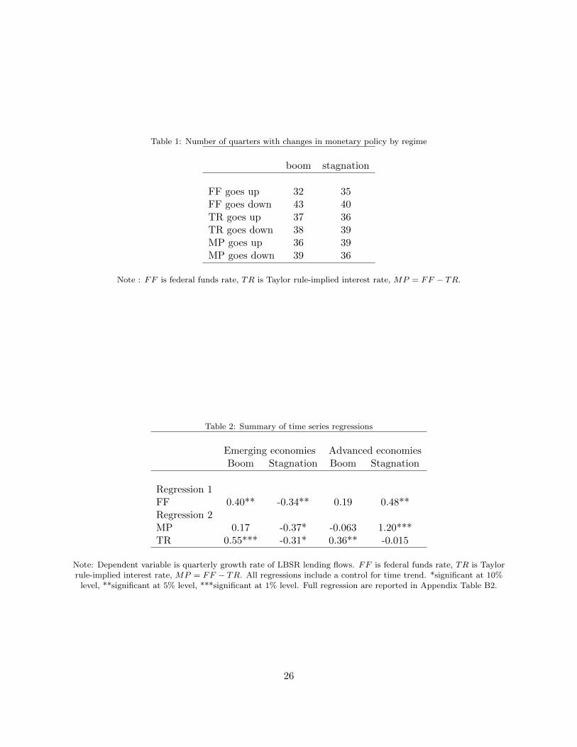
Table 1: Number of quarters with changes in monetary policy by regime

boom stagnation

FF goes up 32 35FF goes down 43 40TR goes up 37 36TR goes down 38 39MP goes up 36 39MP goes down 39 36

Note : FF is federal funds rate, TR is Taylor rule-implied interest rate, MP = FF − TR.

Table 2: Summary of time series regressions

Emerging economies Advanced economiesBoom Stagnation Boom Stagnation

Regression 1FF 0.40** -0.34** 0.19 0.48**Regression 2MP 0.17 -0.37* -0.063 1.20***TR 0.55*** -0.31* 0.36** -0.015

Note: Dependent variable is quarterly growth rate of LBSR lending flows. FF is federal funds rate, TR is Taylorrule-implied interest rate, MP = FF − TR. All regressions include a control for time trend. *significant at 10%

level, **significant at 5% level, ***significant at 1% level. Full regression are reported in Appendix Table B2.

26

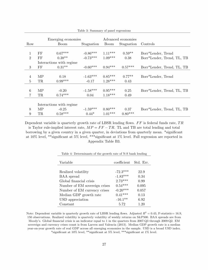
Table 3: Summary of panel regressions

Emerging economies Advanced economiesRow Boom Stagnation Boom Stagnation Controls

1 FF 0.67*** -0.86*** 1.11*** 0.59** Borr*Lender, Trend2 FF 0.38** -0.73*** 1.09*** 0.38 Borr*Lender, Trend, TL, TB

Interactions with regime3 FF 0.31** -0.60*** 0.94*** 0.57*** Borr*Lender, Trend, TL, TB

4 MP 0.18 -1.63*** 0.85*** 0.77** Borr*Lender, Trend5 TR 0.99*** -0.17 1.28*** 0.43

6 MP -0.20 -1.58*** 0.95*** 0.25 Borr*Lender, Trend, TL, TB7 TR 0.74*** 0.04 1.18*** 0.49

Interactions with regime8 MP -0.25 -1.59*** 0.80*** 0.37 Borr*Lender, Trend, TL, TB9 TR 0.58*** 0.44* 1.01*** 0.80***

Dependent variable is quarterly growth rate of LBSR lending flows. FF is federal funds rate, TRis Taylor rule-implied interest rate, MP = FF − TR. TL and TB are total lending and total

borrowing by a given country in a given quarter, in deviations from quarterly mean. *significantat 10% level, **significant at 5% level, ***significant at 1% level. Full regression are reported in

Appendix Table B3.

Table 4: Determinants of the growth rate of N-S bank lending

Variable coefficient Std. Err.

Realized volatility -72.3*** 22.9BAA spread -1.83*** 0.34Global financial crisis 2.73*** 0.99Number of EM sovereign crises 0.54*** 0.095Number of EM currency crises -0.20*** 0.057Median GDP growth rate 0.41*** 0.13USD appreciation -16.1** 6.92Constant 5.72 1.20

Note: Dependent variable is quarterly growth rate of LBSR lending flows. Adjusted R2 = 0.43, F-statistic= 16.9,150 observations. Realized volatility is quarterly volatility of weekly returns on S&P500. BAA spreads are fromMoody’s. Global financial crisis is an indicator equal to 1 in the quarters from 2007:Q3 through 2009:Q2. EMsovereign and currency crises count is from Laeven and Valencia (2013). Median GDP growth rate is a medianyear-on-year growth rate of real GDP across all emerging economies in the sample. USD is a broad USD index.

*significant at 10% level, **significant at 5% level, ***significant at 1% level.

27

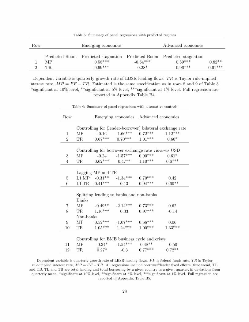
Table 5: Summary of panel regressions with predicted regimes

Row Emerging economies Advanced economies

Predicted Boom Predicted stagnation Predicted Boom Predicted stagnation1 MP 0.58*** -0.64*** 0.59*** 0.82**2 TR 0.99*** 0.28* 0.96*** 0.61***

Dependent variable is quarterly growth rate of LBSR lending flows. TR is Taylor rule-impliedinterest rate, MP = FF − TR. Estimated is the same specification as in rows 8 and 9 of Table 3.*significant at 10% level, **significant at 5% level, ***significant at 1% level. Full regression are

reported in Appendix Table B4.

Table 6: Summary of panel regressions with alternative controls

Row Emerging economies Advanced economies

Controlling for (lender-borrower) bilateral exchange rate1 MP -0.16 -1.66*** 0.72*** 1.12***2 TR 0.67*** 0.70*** 1.01*** 0.60*

Controlling for borrower exchange rate vis-a-vis USD3 MP -0.24 -1.57*** 0.90*** 0.61*4 TR 0.62*** 0.47** 1.10*** 0.67**

Lagging MP and TR5 L1.MP -0.31** -1.34*** 0.70*** 0.426 L1.TR 0.41*** 0.13 0.94*** 0.60**

Splitting lending to banks and non-banksBanks

7 MP -0.49** -2.14*** 0.73*** 0.628 TR 1.16*** 0.33 0.97*** -0.14

Non-banks9 MP 0.52*** -1.07*** 0.66*** 0.0610 TR 1.05*** 1.24*** 1.00*** 1.33***

Controlling for EME business cycle and crises11 MP -0.34* -1.54*** 0.48** -0.5012 TR 0.27* -0.3 0.77*** 0.72**

Dependent variable is quarterly growth rate of LBSR lending flows. FF is federal funds rate, TR is Taylorrule-implied interest rate, MP = FF − TR. All regressions include borrower*lender fixed effects, time trend, TL

and TB. TL and TB are total lending and total borrowing by a given country in a given quarter, in deviations fromquarterly mean. *significant at 10% level, **significant at 5% level, ***significant at 1% level. Full regression are

reported in Appendix Table B5.

28

Appendix A: Country Lists

Lenders

Australia, Austria, Bahamas, Bahrain, Belgium, Bermuda, Brazil, Canada, Cayman Islands, Chile, Chinese Taipei, Curaçao, Cyprus, Denmark, Finland, France, Germany, Greece, Guernsey, Hong Kong SAR, India, Indonesia, Ireland, Isle of Man, Italy, Japan, Jersey, Luxembourg, Macao SAR, Malaysia, Mexico, Netherlands, Netherlands Antilles, Norway, Panama, Portugal, Singapore, South Africa, South Korea, Spain, Sweden, Switzerland, Turkey, United Kingdom and United States.

Advanced economy borrowers

Andorra, Australia, Austria, Belgium, Canada, Cyprus, Denmark, Estonia, Finland, France, Germany, Greece, Iceland, Ireland, Italy, Japan, Latvia, Liechtenstein, Lithuania, Luxembourg, Malta, Netherlands, New Zealand, Norway, Portugal, Slovakia, Slovenia, Spain, Sweden, Switzerland, United Kingdom and United States.

Emerging market economy borrowers

Algeria, Angola, Argentina, Azerbaijan, Bangladesh, Belarus, Belize, Brazil, Bulgaria, Cambodia, Chile, China, Chinese Taipei, Colombia, Costa Rica, Croatia, Czech Republic, Dominican Republic, Ecuador, Egypt, El Salvador, Ghana, Guatemala, Honduras, Hungary, India, Indonesia, Iran, Israel, Jamaica, Jordan, Kazakhstan, Kenya, Kuwait, Liberia, Malaysia, Marshall Islands, Mexico, Morocco, Mozambique, New Caledonia, Nigeria, Oman, Pakistan, Paraguay, Peru, Philippines, Poland, Qatar, Romania, Russia, Saudi Arabia, Serbia, Seychelles, South Africa, South Korea, Sri Lanka, Tanzania, Thailand, Trinidad and Tobago, Tunisia, Turkey, Ukraine, United Arab Emirates, Uruguay, Venezuela, Vietnam and Zambia.

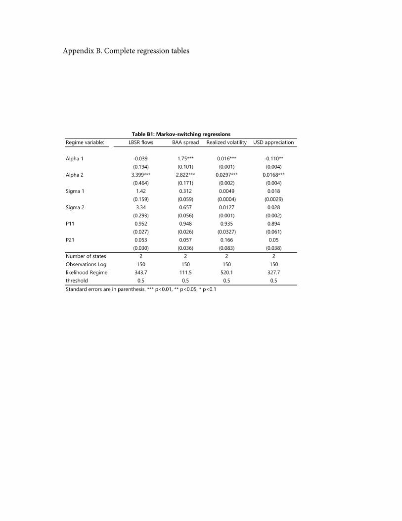
Regime variable: LBSR flows BAA spread Realized volatility USD appreciation

Alpha 1 -0.039 1.75*** 0.016*** -0.110**(0.194) (0.101) (0.001) (0.004)

Alpha 2 3.399*** 2.822*** 0.0297*** 0.0168***(0.464) (0.171) (0.002) (0.004)

Sigma 1 1.42 0.312 0.0049 0.018(0.159) (0.059) (0.0004) (0.0029)

Sigma 2 3.34 0.657 0.0127 0.028(0.293) (0.056) (0.001) (0.002)

P11 0.952 0.948 0.935 0.894(0.027) (0.026) (0.0327) (0.061)

P21 0.053 0.057 0.166 0.05(0.030) (0.036) (0.083) (0.038)

2 2 2 2150 150 150 150

343.7 111.5 520.1 327.7

Number of states Observations Log likelihood Regime threshold 0.5 0.5 0.5 0.5

Table B1: Markov-switching regressions

Standard errors are in parenthesis. *** p<0.01, ** p<0.05, * p<0.1

Appendix B. Complete regression tables

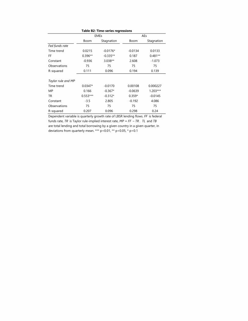
Boom Stagnation Boom StagnationFed funds rateTime trend 0.0215 -0.0176* -0.0134 0.0133FF 0.396** -0.335** 0.187 0.481**Constant -0.936 3.038** 2.608 -1.073Observations 75 75 75 75R-squared 0.111 0.096 0.194 0.139

0.0347* -0.0170 0.00108 0.0002270.166 -0.367* -0.0639 1.203***

0.553*** -0.312* 0.359* -0.0145-3.5 2.805 -0.192 4.08675 75 75 75

Taylor rule and MP Time trendMPTRConstant ObservationsR-squared 0.207 0.096 0.298 0.24Dependent variable is quarterly growth rate of LBSR lending flows. FF is federal funds rate, TR is Taylor rule-implied interest rate, MP = FF – TR . TL and TB are total lending and total borrowing by a given country in a given quarter, in deviations from quarterly mean. *** p<0.01, ** p<0.05, * p<0.1

Table B2: Time-series regressionsEMEs AEs

EMEs

AEs

Boom

Stag

natio

nBo

omSt

agna

tion

Boom

Stag

natio

nBo

omSt

agna

tion

Fed

fund

s ra

teTi

me

tren

d0.

0765

***

-0.0

0189

0.05

65**

0.05

33**

0.03

72**

0.00

706

0.05

67**

0.02

980.

0298

**0.

0444

***

Boom

regi

me

-1.8

7***

-0.8

18FF

(Boo

m)

0.30

9**

0.93

9***

FF (S

tagn

atio

n)-0

.597

***

0.57

2***

TL21

.9**

*8.

90**

*80

.9**

*65

.8**

*14

.7**

*74

.9**

*TB

74.2

***

54.9

***

68.3

***

51.2

***

64**

*60

.7**

*FF

0.66

7***

-0.8

62**

*1.

11**

*0.

594*

*0.

378*

*-0

.731

***

1.09

***

0.37

5

Obs

erva

tions

90,0

4187

,773

54,9

2351

,147

90,0

4187

,773

54,9

2351

,147

177,

884

106,

085

R-sq

uare

d0.

046

0.06

50.

052

0.06

10.

056

0.07

10.

064

0.06

90.

042

0.05

1

Tayl

or ru

le a

nd M

PTi

me

tren

d0.

0961

***

0.00

296

0.06

72**

*0.

0520

**0.

0588

***

0.01

210.

0625

***

0.03

060.

0436

***

0.04

80**

*Bo

om re

gim

e3.

55**

0.25

1M

P (B

oom

)-0

.249

0.80

2***

MP

(Sta

gnat

ion)

-1.5

9***

0.36

5TR

(Boo

m)

0.58

2***

1.01

***

TR (S

tagn

atio

n)0.

442*

0.80

0***

TL22

.7**

*9.

42**

*80

.9**

*65

.9**

*15

.4**

*74

.9**

*TB

74.1

***

54.8

***

68**

*51

.2**

*64

***

60.6

***

MP

0.17

5-1

.63*

**0.

845*

**0.

770*

*-0

.199

-1.5

8***

0.94

8***

0.25

1TR

0.98

6***

-0.1

661.

28**

*0.

432

0.73

8***

0.04

071.

18**

*0.

489

Obs

erva

tions

90,0

4187

,773

54,9

2351

,147

90,0

4187

,773

54,9

2351

,147

177,

884

106,

085

R-sq

uare

d0.

046

0.06

50.

052

0.06

10.

057

0.07

10.

064

0.06

90.

042

0.05

1

Tabl

e B3

: Pan

el r

egre

ssio

ns

Dep

ende

nt v

aria

ble

is q

uart

erly

gro

wth

rate

of L

BSR

lend

ing

flow

s. FF

is fe

dera

l fun

ds ra

te, T

R is

Tay

lor r

ule-

impl

ied

inte

rest

rate

, MP

= F

F –

TR. A

ll re

gres

sion

s in

clud

e bo

rrow

er*l

ende

r fix

ed e

ffect

s. TL

and

TB

are

tota

l len

ding

and

tota

l bor

row

ing

by a

giv

en c

ount

ry in

a g

iven

qua

rter

, in

devi

atio

ns fr

om q

uart

erly

mea

n.**

* p<

0.01

, **

p<0.

05, *

p<

0.1

EMEs

AEs

EMEs

AEs

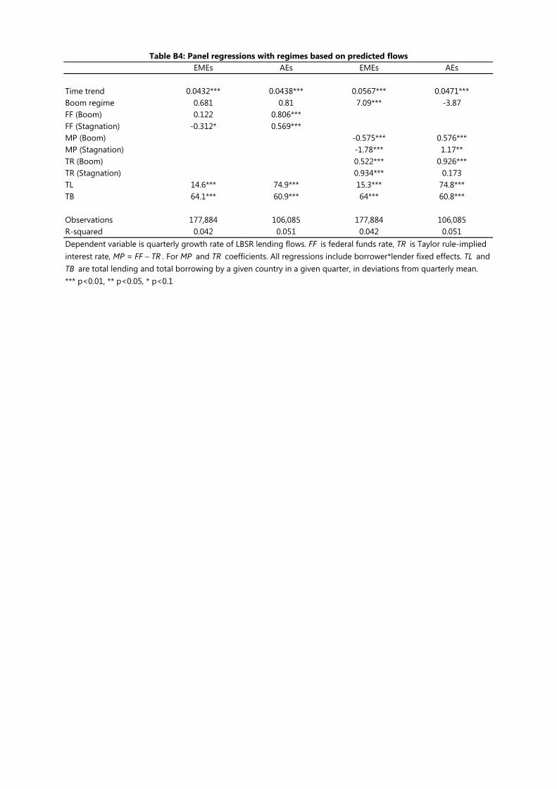
EMEs AEs EMEs AEs

Time trend 0.0432*** 0.0438*** 0.0567*** 0.0471***Boom regime 0.681 0.81 7.09*** -3.87FF (Boom) 0.122 0.806***FF (Stagnation) -0.312* 0.569***MP (Boom) -0.575*** 0.576***MP (Stagnation) -1.78*** 1.17**TR (Boom) 0.522*** 0.926***TR (Stagnation) 0.934*** 0.173TL 14.6*** 74.9*** 15.3*** 74.8***TB 64.1*** 60.9*** 64*** 60.8***

Observations 177,884 106,085 177,884 106,085R-squared 0.042 0.051 0.042 0.051Dependent variable is quarterly growth rate of LBSR lending flows. FF is federal funds rate, TR is Taylor rule-implied interest rate, MP = FF – TR . For MP and TR coefficients. All regressions include borrower*lender fixed effects. TL and TB are total lending and total borrowing by a given country in a given quarter, in deviations from quarterly mean.*** p<0.01, ** p<0.05, * p<0.1

Table B4: Panel regressions with regimes based on predicted flows

EMEs

AEs

EMEs

AEs

EMEs

AEs

EMEs

AEs

EMEs

AEs

EMEs

AEs

Tim

e tr

end

0.05

24**

*0.

0416

**0.

0447

***

0.05

62**

*0.

0315

**0.

0394

**0.

145*

**0.

0627

***

0.08

93**

*0.

0598

***

-0.0

349*

0.04

41*

Boom

regi

me

4.71

**-2

.87

3.52

**-1

.37

2.21

-0.6

730.

566

-6.3

3**

5.28

***

3.31

0.49

33.

3M

P (B

oom

)-0

.164

0.71

6***

-0.2

370.

899*

**-0

.492

**0.

734*

**0.

516*

**0.

664*

**-0

.344

*0.

482*

*M

P (S

tagn

atio

n)-1

.66*

**1.

12**

*-1

.57*

**0.

607*

-2.1

4***

0.62

4-1

.07*

**0.

0574

-1.5

4***

-0.4

99TR

(Boo

m)

0.66

5***

1.01

***

0.61

5***

1.10

***

1.16

***

0.96

6***

1.05

***

0.99

5***

0.26

5*0.

774*

**TR

(Sta

gnat

ion)

0.69

8***

0.60

0*0.

472*

*0.

669*

*0.

330

-0.1

351.

24**

*1.

33**

*-0

.301

0.71

9**

L1.M

P (B

oom

)-0

.305

**0.

701*

**L1

.MP

(Sta

gnat

ion)

-1.3

4***

0.41

5L1

.TR

(Boo

m)

0.40

9***

0.94

0***

L1.T

R (S

tagn

atio

n)0.

130

0.60

2**

Bila

tera

l exc

hang

e ra

te0.

0000

697

0.00

071

Borr

ower

exc

hang

e ra

te v

av U

SD-0

.184

-14.

4**

TL13

.9**

*75

.0**

*15

.4**

*75

.4**

*15

.2**

*75

***

28.8

***

85.3

***

7.49

***

16.4

***

16.1

***

74.8

***

TB70

.6**

*59

.4**

*70

***

60.4

***

64.3

***

60.8

***

13.1

***

8.19

***

34.1

***

51.5

***

63.4

***

61.4

***

Gro

wth

of m

iddl

e in

com

e ec

onom

ies

0.58

2***

0.59

3***

Com

mod

ities

: Met

al0.

0201

***

0.00

777*

*Co

mm

oditi

es: T

extil

e-0

.007

46-0

.016

4Co

mm

oditi

es: F

ood

-0.0

233*

*-0

.031

3**

Com

mod

ities

: Oil

-0.0

56**

-0.0

407

Sove

reig

n de

bt c

rises

-0.2

14-0

.070

3Cu

rren

cy c

rises

0.08

330.

154*

Obs

erva

tions

148,

851

89,4

8417

5,94

910

5,92

617

7,88

410

6,08

513

9,50

998

,923

157,

172

97,7

2117

7,88

410

6,08

5R-

squa

red

0.04

40.

053

0.04

30.

051

0.04

20.

051

0.04

20.

052

0.03

60.

037

0.04

30.

051

With

EM

E co

ntro

ls

Dep

ende

nt v

aria

ble

is q

uart

erly

gro

wth

rate

of L

BSR

lend

ing

flow

s. XR

is

exch

ange

rate

, FF

is fe

dera

l fun

ds ra

te, T

R is

Tay

lor r

ule-

impl

ied

inte

rest

rate

, MP

= F

F –

TR. A

ll re

gres

sion

s in

clud

e bo

rrow

er*l

ende

r fix

ed e

ffect

s. TL

and

TB

are

tota

l len

ding

and

tota

l bor

row

ing

by a

giv

en c

ount

ry in

a g

iven

qua

rter

, in

devi

atio

ns fr

om q

uart

erly

mea

n. G

row

th o

f mid

dle

inco

me

econ

omie

s in

dica

tes

the

Wor

ld B

ank'

s gr

owth

ra

te fo

r mid

dle

inco

me

econ

omie

s. So

vere

ign

debt

cris

es a

nd c

urre

ncy

cris

es a

re d

umm

ies,

equa

l to

one

whe

n th

ere

is a

sov

erei

gn d

ebt o

r cur

renc

y cr

isis

, res

peci

tvel

y, in

an

EME.

***

p<

0.01

, **

p<0.

05, *

p<

0.1

Tabl

e B5

: Pan

el r

egre

ssio

ns w

ith

alte

rnat

ive

cont

rols Le

ndin

g to

ban

ksLe

ndin

g to

non

-ban

ksLa

ggin

g M

P an

d TR

With

bor

row

er X

R va

v U

SDW

ith b

ilate

ral X

R