Uplink Practical Capacity and Interference Statistics of ...journals.tubitak.gov.tr/elektrik/issues/elk-06-14-2/elk-14-2-8... · Turk J Elec Engin, VOL.14, NO.2 2006, c TUB¨ _ITAK

Turk J Elec Engin, VOL.14, NO.2 2006, c© TUBITAK

Uplink Practical Capacity and Interference Statistics

of WCDMA Cigar-shaped Microcells for Highways in

Rural Zones with Non-Uniform Spatial Traffic

Distribution and Imperfect Power Control

Bazil TAHA-AHMED, Miguel CALVO-RAMON and Leandro de HARO-ARIETDepartamento Sistemas, Senales y Radiocomunicaciones,

ETSI Telecomunicacion, Universidad Politecnica de MadridCiudad Universitaria, Madrid, 28040

e-mail: [email protected]

Abstract

The capacity (the maximum number of users per sector that the system can support) and the interfer-

ence statistics (expected value and variance) of sectors composed of cigar-shaped WCDMA microcells are

studied. A model of 5 microcells is used to analyze the uplink capacity and interference statistics. The

microcells are assumed to exist in rural zone highways. The capacity and the interference statistics of the

microcells are studied for different non-uniform spatial traffic distributions. As user density decreases

away from the base station, the capacity of the sector increases due to the reduced total power transmitted

by the interfering users.

Key Words: W-CDMA, uplink capacity, shadowing.

1. Introduction

Microcellular systems have been proposed to increase cellular capacity mainly in dense urban areas that havea large volume of wireless communication traffic, or to provide communications service along rural highwayzones. It is well known that CDMA is characterized as interference-limited, so reducing the interferenceresults in increased capacity. Three techniques are used to reduce the interference: power control (PC),which is essential in the uplink; voice activity monitoring; and sectorization. Also, well known is that urbanand rural microcell shapes may approximately follow street layouts and that it is also possible to have cigar-shaped microcells [1]. Conditions that direct the design of cigar-shaped microcells for highways in ruralzones are:

• each cigar-shaped microcell is formed from two directive sectors, a directive antenna signaling eachsector;

• each sector should have a typical range of 1 to 1.5 km;

• user speed in rural areas can reach 120 km/h and above.

329

Turk J Elec Engin, VOL.14, NO.2, 2006

Figure 1 depicts the radiation pattern of the sector antenna and of the cigar-shaped microcell coverage.From Figure 1A notice that interference from the right side of the sector is injected through the main lobeof the antenna while interference from the left side of the antenna is injected via the side lobe.

Main lobe Side lobe

A

B

Base station (2 sectors) Sector 1 coverageSector 2 coverage Base station (2 sectors) Sector 1 coverageSector 2 coverage

Figure 1. The sector antenna radiation pattern and microcell coverage. (a) The radiation pattern of the sector’s

antenna. (b) The cigar-shaped microcell coverage.

In the real world, it is rather uncommon to see spatially uniform traffic in macro- and microcells. Yetthe majority of WCDMA cells have been designed to assume uniform spatial distribution: an unrealisticpractice.

Min et al. studied the performance of the CDMA highway microcell using one slope propagationmodel and two slope propagation model without taking into account the interference variance nor the non-uniform spatial distribution of users [2]. Hashem et al. studied the capacity and the interference statistics

for hexagonal cell for a propagation exponent of 4 and a uniform spatial distribution of users [3]. In [4], thecapacity, the mean and variance statistics of interference of cigar-shaped microcells for highways in ruralzones using wide-band code-division multiple access (WCDMA) have been studied. A general propagationexponent using a two-slope propagation model and log-normal shadowing was used. It has been assumedthat users are uniformly distributed within the microcells, that the intracellular interference variance is nulland that the power control is perfect.

In this work, we will use a model for cigar-shaped microcells in rural highways zones with generalpropagation exponent using a two-slope model and then investigate the sector capacity and interferencestatistics of the uplink for different spatial distributions of users and different standard deviation error inpower control.

The paper has been organized as follows. In section 2, the propagation model is given. Section 3explains the method to calculate the capacity and the interference statistics of the uplink. Numerical results

330

TAHA-AHMED, CALVO-RAMON, HARO-ARIET: Uplink Practical Capacity and...,

are presented in section 4. Finally, in section 5 conclusions are drawn.

2. The Propagation Model

A two-slope propagation model with lognormal shadowing is used in our calculations [2]. The exponent ofthe propagation is assumed to be s1 up to the break point Rb , above which it converts into s2 . In this waythe path loss at a distance r from the base station is given by [4]

Lp(dB) ≈ Lb + 10 + 10 s1 log10

(r

Rb

)+ ξ1 for r ≤ Rb (1)

Lp(dB) ≈ Lb + 10 + 10 s2 log10

(r

Rb

)+ ξ2 for r > Rb, (2)

where r is the distance between the microcell base station and the mobile; and Lb (defined as the propagation

loss at Rb ) and Rb are given by [5]

Lb(dB) =

∣∣∣∣∣ 10 log

[(λ2

8π hb hm

)2] ∣∣∣∣∣ (3)

Rb ≈4 hb hmλ

. (4)

Here, hb is the base station antenna height; hm is the mobile antenna height; λ is the wavelength;and ξ1 and ξ2 are Gaussian random variables of zero-mean and standard deviation σ1 and σ2 , respectively.In practice, ξ1 and ξ2 are truncated to ±10 dB.

Typical values for s1 , s2 , σ1 and σ2 are:

• s1 = 1.75 to 2.25• s2 = 3.50 to 4.75• σ1 = 2 to 3 dB• σ2 = 4 to 6 dB.

3. Uplink Capacity and Interference Analysis

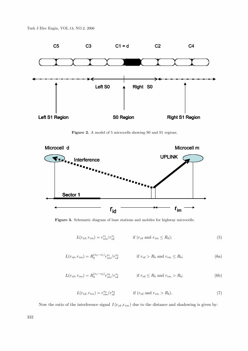
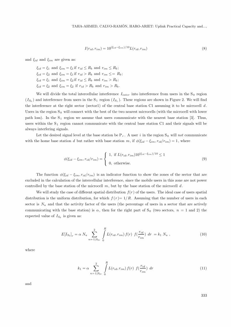
In cigar-shaped microcells for highways, the sector range (radio) is typically 1 to 1.5 km and the highwaywidth is 10 to 16 m. Thus, the cigar-shaped microcell can be treated as a one-dimension microcell. Toassess the sector capacity, we have to calculate the expected value and the variance of the total interference(intracellular + intercellular) and then we model the total interference as a Gaussian noise. Figure 2 a model

configuration of 5 collinear microcells (i.e. ten sectors) used in the analysis of the uplink sector capacity.Each microcell controls the transmitted power of its users. The sector range is assumed to be R . If theinterfering user i is at a distance rim from its base station (m) and at a distance rid from the home microcell

base station d, as shown in Figure 3, then the ratio of the interference signal L(rid , rim ) due to the distance

only is given as [4]

331


Left S1 Region S0 Region Right S1 Region

Left S0 Right S0

C5 C3 C1 = d C2 C4


Left S0 Right S0

C5 C3 C1 = d C2 C4


Left S0 Right S0


Left S0 Right S0

Left S1 Region S0 Region Right S1 RegionLeft S1 Region S0 Region Right S1 Region

Left S0 Right S0

C5 C3 C1 = d C2 C4

Figure 2. A model of 5 microcells showing S0 and S1 regions.

Sector 1

ridrim

Microcell d Microcell m

InterferenceUPLINK

Sector 1

ridrim


Sector 1

ridrim

Sector 1

rid

Sector 1 Sector 1 Sector 1

ridrim


InterferenceUPLINK

InterferenceInterferenceUPLINKUPLINK

Figure 3. Schematic diagram of base stations and mobiles for highway microcells.

L(rid, rim) = rs1im/r

s1id if (rid and rim ≤ Rb); (5)

L(rid, rim) = R(s2−s1)b rs1

im/rs2id if rid > Rb and rim ≤ Rb; (6a)

L(rid, rim) = R(s1−s2)b rs2

im/rs1id if rid ≤ Rb and rim > Rb; (6b)

L(rid, rim) = rs2im/r

s2id if (rid and rim > Rb). (7)

Now the ratio of the interference signal I (r id ,r im ) due to the distance and shadowing is given by:

332


I(rid, rim) = 10(ξid−ξim)/10L(rid, rim) (8)

and ξid and ξim are given as:

ξid = ξ1 and ξim = ξ1 if rid ≤ Rb and rim ≤ Rb ;

ξid = ξ2 and ξim = ξ1 if rid > Rb and rim ≤= Rb ;

ξid = ξ1 and ξim = ξ2 if rid ≤ Rb and rim > Rb ;

ξid = ξ2 and ξim = ξ2 if rid > Rb and rim > Rb .

We will divide the total intercellular interference Iinter into interference from users in the S0 region(IS0 ) and interference from users in the S1 region (IS1 ). These regions are shown in Figure 2. We will find

the interference at the right sector (sector1) of the central base station C1 assuming it to be microcell d .

Users in the region S0 will connect with the best of the two nearest microcells (with the microcell with lower

path loss). In the S1 region we assume that users communicate with the nearest base station [3]. Thus,users within the S1 region cannot communicate with the central base station C1 and their signals will bealways interfering signals.

Let the desired signal level at the base station be Pr . A user i in the region S0 will not communicatewith the home base station d but rather with base station m , if φ(ξid − ξim, rid/rim) = 1, where

φ(ξid − ξim, rid/rim) =

1, if L(rid, rim)10(ξid−ξim)/10 ≤ 1

0, otherwise.(9)

The function φ(ξid − ξim, rid/rim) is an indicator function to show the zones of the sector that areexcluded in the calculation of the intercellular interference, since the mobile users in this zone are not powercontrolled by the base station of the microcell m , but by the base station of the microcell d .

We will study the case of different spatial distribution f(r ) of the users. The ideal case of users spatial

distribution is the uniform distribution, for which f (r )= 1/R . Assuming that the number of users in each

sector is Nu and that the activity factor of the users (the percentage of users in a sector that are actively

communicating with the base station) is α , then for the right part of S0 (two sectors, n = 1 and 2) theexpected value of IS0 is given as:

E[IS0 ]r = α Nu

2∑n=1|S0r

R∫0

L(rid, rim) f(r) f(ridrim

) dr = k1 Nu , (10)

where

k1 = α

2∑n=1|S0r

R∫0

L(rid, rim) f(r) f(ridrim

) dr (11)

and

333


f(ridrim

) = E[10(ξid−ξim)/10φ(ξid − ξim, rid/rim)

](12)

= e(βσ)2/2Q

[β√σ2 − 10√

σ2log10 {1/L(rid, rim)}

]. (13)

Here, β = 110 log 10 and Q(x) is given by

Q(x) =

∞∫x

e−v2/2dv/

√2π. (14)

In equations (10)–(13), rim and ridhas the following values when the user is in the left and rightsectors:

rim =

r when the user is in left sector C2

2R− r when the user is in right sector C1

rid =

2R− r when the user is in left sector C2

r when the user is in right sector C1.

σid and σim are given as:

σid =

σ1when : rid ≤ Rb

σ2when : rid > Rb(15)

σim =

σ1when : rim ≤ Rb

σ2when : rim > Rb(16)

The general value of σ 2 is given as:

σ2 =

2(1− Cdm)σ2

1 when : rid ≤ Rb and rid ≤ Rb

(σ1 − σ2)2 + 2(1− Cdm)σ1σ2 when : rid ≤ Rb and rim > Rb or rid > Rb and rim ≤ Rb

2(1− Cdm)σ22 when : rid > Rbandrim > Rb

(17)

where Cdm is the correlation coefficient between the random variable ξid and ξim (shadowing correlation

between base stations).

334


The expected value of IS1 due to the right part of the S1 region (summed over the three sectors on

the right, n = 1, . . . , 3) is given as

E[IS1]r ≈ α Nu3∑

n=1|S1r

R∫0

L(rid, rim) f(r) E[10(ξid−ξim)/10

]dr = k2 Nu, (18)

where we define

k2 ≈ α3∑

n=1|S1r

R∫0


]dr (19)

In the integrand of (18), rim takes the value r while ridassumes the value R(2+n)–r .

The expected value of the intercellular interference from the right side of the regions S0 and S1 is

E[I]r = E[IS0 ]r + E[IS1 ]r. (20)

For the left part of S0 (two sectors, numbered n = 1, 2), the expected value of IS0 is given as

E[IS0 ]l = α Sll Nu

2∑n=1|S0l

R∫0

L(rid, rim)fs(r) f(ridrim

) dr = k3 Nu, (21)

where Sll is the side lobe level of the directive antenna used in each sector and k3 is given by

k3 = Sll α2∑

n=1|S0l

R∫0

L(rid, rim)f(r) f(ridrim

) dr (22)

The expected value of IS1 due to left part of the S1 region (three sectors, n =1, . . . , 3) is given as:

E[IS1]l ≈ α Sll Nu3∑

n=1|S1l

R∫0


]dr = k4 Nu (23)

where

k4 ≈ Sll α3∑

n=1|S1l

R∫0


]dr. (24)

Thus the expected value of the total intercellular interference from the left and right sides is given as

E[I]inter = E[IS0]r + E[IS1]r + E[IS0]l + E[IS1]l. (25)

335


The expected value of the total intercellular interference power is given as

E[P ]inter = Pr E[I]inter. (26)

The expected value of the intracellular interference power is given by

E[P ]intra ≈ Pr E[I]intra ≈ α Nu(1 + Sll) Pr = k5 Nu Pr. (27)

Taking into account an imperfect power control with standard deviation error of σc (dB), the expected valueof the total interference power Pt will be

E[P ]t = eβ2σ2c/2(E[P ]intra + E[P ]inter) = kpc (E[P ]intra +E[P ]inter), (28)

where kpc is the power control error factor given by

kpc = eβ2σ2c/2. (29)

In the uplink, only εPr of Pr is used in the demodulation (ε = 14/16 = 0.875 or ε = 15/16 = 0.9375) [7].

Thus, the expected value of the uplink carrier-to-interference ratio (C/I) is given as

[C/I] =ε PrE[P ]t

(30)

and the value of the energy per bit to noise ratio (Eb / No ) is given as

[Eb/No] = [C/I] ∗Gp, (31)

where Gp is the processing gain. That is,

[Eb/No] =ε Gp

Nu kpc (k1 + k2 + k3 + k4 + k5)(32)

N =ε Gp

[Eb/No]req kpc (k1 + k2 + k3 + k4 + k5), (33)

where N is the expected value of the number of users per sector (expressed as the average capacity) and

(Eb /No )req is the required (Eb /No ) to get a given bit error rate for a given service.

Assuming a user traveling at 120 km/h and transmitting/receiving at 9.6 kbit/sec, the signal-to-nose

ratio (Eb /No )req must be ≥7 dB. For a bit rate of 144 kbit/sec, the relation (Eb /No )req has to be ≥3

dB [6].

The variance in IS0 at the right part of S0 (two sectors) is computed as

336


var[IS0]r = Nu

2∑n=1|S0r

R∫0

[L(rid, rim)]2 [f(r)]{pα g(

rdrm

) − qα2f2(rdrm

)}dr, (34)

where

g(rdrm

) = E[10(ξid−ξim)/10φ(ξid − ξim, rid/rim)

] 2

(35)

= e2(βσ)2Q

[√σ2 ln 10/5− 10√

σ2log10 {1/L(rid, rim)}

](36)

p = e2β2σ2c (37)

q = eβ2σ2c . (38)

The variance of IS1 due to right part of S1 (three sectors) is given as

var[IS1]r ≈ Nu3∑

n=1|S1r

R∫0

[L(rid, rim)]2 [f(r)] ·{pαE

[(10(ξid−ξim)/10)2

]− qα2E2

[10(ξid−ξim)/10

] }dr

(39)

The variance of IS0 due to left part of S0 (two sectors) is given as

var[IS0]l = Sll Nu

2∑n=1|S0l

R∫0

[L(rid, rim)]2 [f(r)]{pαg(

rdrm

)− qα2f2(rdrm

)}dr. (40)

The variance of IS1 due to left part of S1 (three sectors) is given as:

var[IS1]l ≈ Sll Nu3∑

n=1|S1l

R∫0

[L(rid, rim)]2 [f(r)] ·{pαE

[(10(ξid−ξim)/10)2

]− qα2E2

[10(ξid−ξim)/10

] }dr

(41)

Thus the sum of intercellular variance due to regions S0 and S1 is given by

var[I]inter = { var[IS0]r + var[IS1]r }+ {var[IS0]l + var[IS1]l }. (42)

The intracellular interference variance is calculated as

337


var[I]intra ≈ Nu (1 + Sll)(pα− qα2

). (43)

The total interference variance is given by the sum

var[I]t = var[I]inter + var[I]intra. (44)

The total interference power variance is given by the relation

var[Pintf ]t = P 2var[I]t. (45)

Finally, we calculate the probability for outage, that is, the probability that the signal-to-noise ratioof a percentage of users does not reach the required Eb /No threshold. To do so, we need the medium value

of the interference, i.e. the interference when the number of users per sector is N , the expected value andthe variance of the interference when the number of users per sector is Nu . The outage probability is givenby the relation

Pr = Q

[E(I)t|−

N−E(I)t|Nu√

var(I) t|Nu

]. (46)

This Gaussian approximation is valid when the number of users Nu ≥ 20, the number we assume for thiswork.

We calculate the F factor, which expresses the ratio of interference from other microcells to theinterference of the microcell under consideration, as

F =IntercellularInterference

IntracellularInterference=E[P ]interE[P ]intra

(47)

and the effective interference power as

[Pintf ]eff = E[P ]t + γ√var[P ]t, (48)

where γ is the deviation factor and is a function of the accepted outage probability. The practical values ofγ are 2.06 (2% outage, since Q(2.06) = 0.02) to 2.33 (1% outage, since Q(2.33) = 0.01).

4. Numerical Results

Our calculations assume a W-CDMA chip rate of 3.84 Mcps/sec [7], plus the application of other reasonablefigures. The antenna azimuth side lobe level is assumed to be –15 dB, the correlation coefficients Cdm = 0.5[7], s1 = 2, s2 = 4, σ1 = 3 dB, σ2 = 6 dB, R b = 300 m, R = 1000 m, ε = 0.9375 [7] and σc = 1.5

dB, unless otherwise expressly stated. We assume that the accepted outage probability is 1% and that thecapacity of the sectors is calculated at this probability.

338


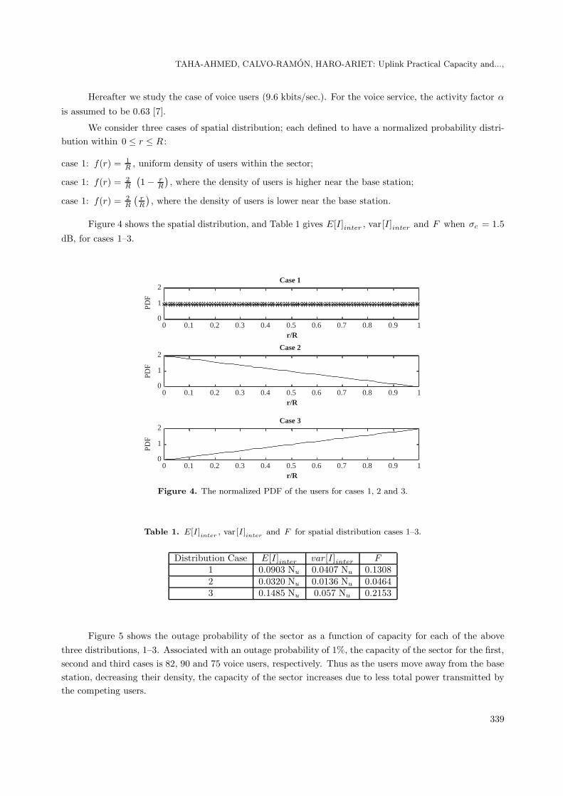
Hereafter we study the case of voice users (9.6 kbits/sec.). For the voice service, the activity factor α

is assumed to be 0.63 [7].

We consider three cases of spatial distribution; each defined to have a normalized probability distri-bution within 0 ≤ r ≤ R :

case 1: f(r) = 1R , uniform density of users within the sector;

case 1: f(r) = 2R

(1− r

R

), where the density of users is higher near the base station;

case 1: f(r) = 2R

(rR

), where the density of users is lower near the base station.

Figure 4 shows the spatial distribution, and Table 1 gives E[I]inter , var[I]inter and F when σc = 1.5

dB, for cases 1–3.

0 0.1 0.2 0.3 0.4 0.5 0.6 0.7 0.8 0.9 10

1

2 Case 1

r/R

0 0.1 0.2 0.3 0.4 0.5 0.6 0.7 0.8 0.9 10

1

2 Case 2

r/R

0 0.1 0.2 0.3 0.4 0.5 0.6 0.7 0.8 0.9 10

1

2 Case 3

r/R

PD

FP

DF

PD

F

Figure 4. The normalized PDF of the users for cases 1, 2 and 3.

Table 1. E[I ]inter , var[I ]inter and F for spatial distribution cases 1–3.

Distribution Case E[I]inter var[I]inter F1 0.0903 Nu 0.0407 Nu 0.13082 0.0320 Nu 0.0136 Nu 0.04643 0.1485 Nu 0.057 Nu 0.2153

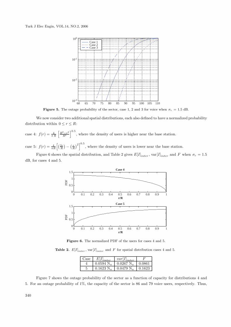
Figure 5 shows the outage probability of the sector as a function of capacity for each of the abovethree distributions, 1–3. Associated with an outage probability of 1%, the capacity of the sector for the first,second and third cases is 82, 90 and 75 voice users, respectively. Thus as the users move away from the basestation, decreasing their density, the capacity of the sector increases due to less total power transmitted bythe competing users.

339


100

10-1

10-2

10-3

Case 1Case 2Case 3

60 65 70 75 80 85 90 95 100 105 110

Figure 5. The outage probability of the sector, case 1, 2 and 3 for voice when σc = 1.5 dB.

We now consider two additional spatial distributions, each also defined to have a normalized probabilitydistribution within 0 ≤ r ≤ R :

case 4: f(r) = 4πR

[R2−r2

R2

]0.5

, where the density of users is higher near the base station.

case 5: f(r) = 4πR

[(2rR

)−(rR

)2]0.5 , where the density of users is lower near the base station.

Figure 6 shows the spatial distribution, and Table 2 gives E[I]inter , var[I]inter and F when σc = 1.5

dB, for cases 4 and 5.

0 0.1 0.2 0.3 0.4 0.5 0.6 0.7 0.8 0.9 10

0.5

1

1.5 Case 4

r/R

0 0.1 0.2 0.3 0.4 0.5 0.6 0.7 0.8 0.9 10

0.5

1

1.5 Case 5

r/R

PD

FP

DF

Figure 6. The normalized PDF of the users for cases 4 and 5.

Table 2. E[I ]inter , var[I ]inter and F for spatial distribution cases 4 and 5.

Case E[I]inter var[I]inter F4 0.0594 Nu 0.0267 Nu 0.08615 0.1623 Nu 0.0479 Nu 0.1623

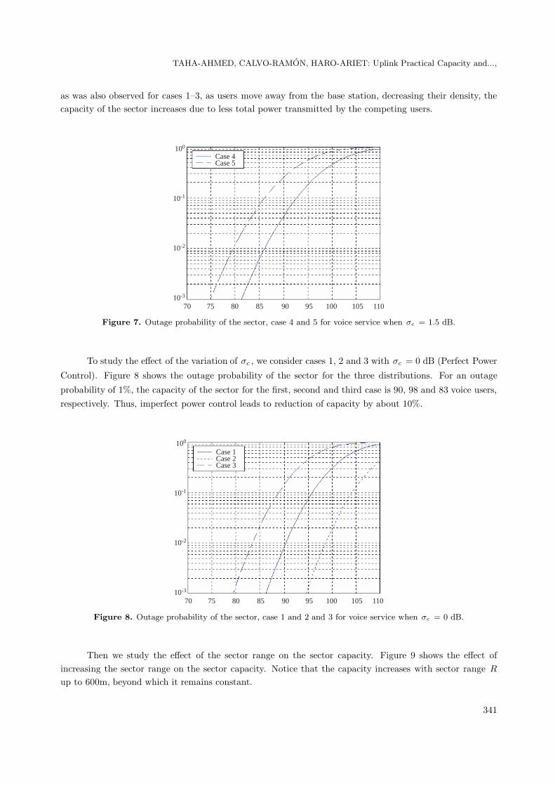
Figure 7 shows the outage probability of the sector as a function of capacity for distributions 4 and5. For an outage probability of 1%, the capacity of the sector is 86 and 79 voice users, respectively. Thus,

340


as was also observed for cases 1–3, as users move away from the base station, decreasing their density, thecapacity of the sector increases due to less total power transmitted by the competing users.

100

10-1

10-2

10-3

Case 4Case 5

70 75 80 85 90 95 100 105 110

Figure 7. Outage probability of the sector, case 4 and 5 for voice service when σc = 1.5 dB.

To study the effect of the variation of σc , we consider cases 1, 2 and 3 with σc = 0 dB (Perfect Power

Control). Figure 8 shows the outage probability of the sector for the three distributions. For an outage

probability of 1%, the capacity of the sector for the first, second and third case is 90, 98 and 83 voice users,respectively. Thus, imperfect power control leads to reduction of capacity by about 10%.

100

10-1

10-2

10-3

Case 1Case 2Case 3

70 75 80 85 90 95 100 105 110

Figure 8. Outage probability of the sector, case 1 and 2 and 3 for voice service when σc = 0 dB.

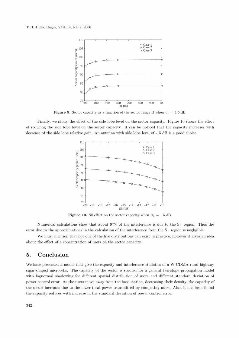
Then we study the effect of the sector range on the sector capacity. Figure 9 shows the effect ofincreasing the sector range on the sector capacity. Notice that the capacity increases with sector range R

up to 600m, beyond which it remains constant.

341


300 400 500 600 700 800 900 10075

80

85

90

95

100

105

110

R (m)

Case 1 Case 2 Case 3

Sec

tor

capa

city

(vo

ice

user

s)

Figure 9. Sector capacity as a function of the sector range R when σc = 1.5 dB.

Finally, we study the effect of the side lobe level on the sector capacity. Figure 10 shows the effectof reducing the side lobe level on the sector capacity. It can be noticed that the capacity increases withdecrease of the side lobe relative gain. An antenna with side lobe level of -15 dB is a good choice.

70

80

85

90

95

100

105

110

Sec

tor

capa

city

(vo

ice

user

s)

-20 -19 -18 -17 -16 -15 -14 -13 -12 -11 -10 Sll (dB)

Case 1 Case 2 Case 3

75

Figure 10. Sll effect on the sector capacity when σc = 1.5 dB.

Numerical calculations show that about 97% of the interference is due to the S0 region. Thus theerror due to the approximations in the calculation of the interference from the S1 region is negligible.

We must mention that not one of the five distributions can exist in practice; however it gives an ideaabout the effect of a concentration of users on the sector capacity.

5. Conclusion

We have presented a model that give the capacity and interference statistics of a W-CDMA rural highwaycigar-shaped microcells. The capacity of the sector is studied for a general two-slope propagation modelwith lognormal shadowing for different spatial distribution of users and different standard deviation ofpower control error. As the users move away from the base station, decreasing their density, the capacity ofthe sector increases due to the lower total power transmitted by competing users. Also, it has been foundthe capacity reduces with increase in the standard deviation of power control error.

342


References

[1] Ho-Shin Cho, Min Young Chung, Sang Hyuk Kang and Dan Keun Sung “Performance Analysis of Cross-and

Cigar Shaped Urban Microcells Considering User mobility Characteristics”, IEEE Veh. Tech., Vol. 49, No. 1,

pp 105-115, Jan. 2000.

[2] Seungwook Min and Henry L. Bertoni “ Effect of Path Loss Model on CDMA System Design for Highway

Microcells “, 48 th VTC, Ottawa, Canada, pp 1009-1013, May 1998.

[3] B. Hashem and E. S. Sousa, “ Reverse Link Capacity and Interference Statistics of a Fixed-step Power-controlled

DS/CDMA System Under Slow Multipath Fading,” IEEE Trans. Commun., vol. 47, pp. 1905-1912, Dec. 1999.

[4] B. T. Ahmed, M. C. Ramon, and L. de H. Ariet, “Capacity and interference statistics of highways W-CDMA

cigar-shaped microcells (uplink analysis),” IEEE Commun. Lett., vol. 6, pp. 172–174, May 2002.

[5] Ywh-Ren Tsai and Jin-Fu Chang, “ Feasibility of Adding a Personal Communications Network to an Existing

Fixed-service Microwave System“, IEEE Trans. Com., Vol. 44, No . 1, pp 76-83, Jan. 1996.

[6] Bruno Melis and Giovanni Romano “ UMTS W-CDMA: Evaluation of Radio Performance by Means of Link

Level Simulations”, IEEE Personal Communications, Vol. 7, No. 3, pp 42-49, June 2000.

[7] H. Holma and A. Toskal, “WCDMA for UMTS”, John Wiley & Sons, 2000.

343

Documents

Uplink Practical Capacity and Interference Statistics of ...journals.tubitak.gov.tr/elektrik/issues/elk-06-14-2/elk-14-2-8... · Turk J Elec Engin, VOL.14, NO.2 2006, c TUB¨ _ITAK