UNSTEADY STATE HEAT TRANSFER

THERMAL DIFFUSIVITIES AND HEAT TRANSFER

COEFFICIENTSObjective

To observe unsteady state heat flow to or from the center of a solid shape

(qualitative, using data acquisition) when a step change is applied to the

temperature at the surface of the shape.

To determine the thermal conductivity of a solids and the heat transfer

coefficient.

By using

Graphical method, analytical transient- temperature heat flow chart,

Method of Separation of variables, and

Polynomial approximation method,

Investigate the effect of shape, size, and material properties on unsteady

heat flow.

Compare the results obtained using the above methods with literature

values, and determine which method is more accurate.

Determine the temperature profiles as a function of position and time.

Investigate the Lumped Thermal Capacitance method of transient

temperature analysis.

∗ The unit consists a stainless steel water bath and integral

flow duct with external water circulating pump.

Apparatus

Adjustment of the thermostat allows the bath to

be set to a constant temperature (T1) before

beginning the experimental procedure.

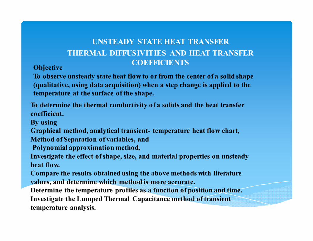
Seven simple shapes of different

materials (Stainless steel and brass) are

provided as shown in Figure below.

Each is fitted with a thermocouples well

at its geometric center and thermocouple

into the carrier to sense water

temperature adjacent to the shape to

allow measurement of its core

temperature (T3) and the surface (T2).

∗ Heat transfer generally takes place by conduction, convection,

and radiation.

Introduction

∗ In absence of internal heat generation, when a cool, solid body is

placed in a warm environment, energy in the form of heat flows

into the body until it attains a thermal equilibrium with its

surroundings.

∗ Starting at time, t = 0, the temperature at any point in the solid is uniform, and increases until the body reaches an isothermal steady state.

∗ The period of time required for the body to reach steady state is a function of the size, shape, and physical properties of the body as well as the conditions imposed on the surface of the body by the experimental conditions

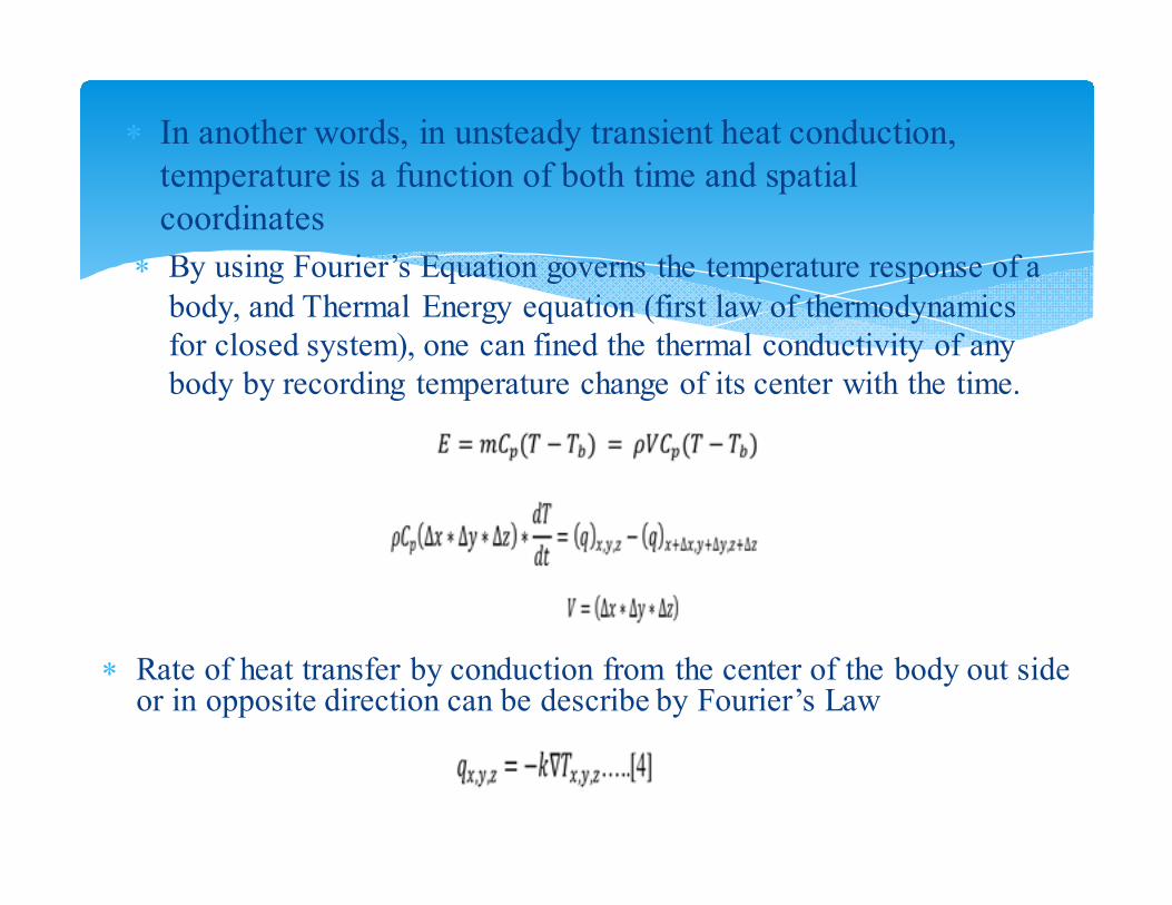
∗ In another words, in unsteady transient heat conduction,

temperature is a function of both time and spatial

coordinates

∗ By using Fourier’s Equation governs the temperature response of a

body, and Thermal Energy equation (first law of thermodynamics

for closed system), one can fined the thermal conductivity of any

body by recording temperature change of its center with the time.

∗ Rate of heat transfer by conduction from the center of the body out side or in opposite direction can be describe by Fourier’s Law

∗ When the body is a metal semi infinite slab or cylinder

or sphere, for one-dimensional case the governing

energy equation is:

Where for slab m=0

for cylinder m=1

for sphere m=2

From thermodynamics definition of the thermal diffusivity

The general governing

convective equation may be

modified to:

∗ How can we characterize the object and the Environment

∗ If the body thermal conductivity is high or the body volume is small, then the temperature response is very fast.

∗ The temperature’s response is a function the internal resistance of the body material.

∗ If the convection coefficient is very high, then the surface temperature of the body becomes very quickly identical to the surrounding temperature.

∗ Alternatively, for a low convection coefficient a large temperature difference exists between the surface and the surrounding.

∗ The value of the coefficient controls what is known as the surface resistance to heat transfer.

∗ In conclusion the instantaneous temperature variation within the system is dependent on the internal and surface resistances.

∗ The larger internal resistance or the smaller surface resistance, the larger temperature variation within the system, and vice versa.

We know the heat transfer in the body mass by conduction to the surface should equal to the heat transfer from the body surface to the surrounding.

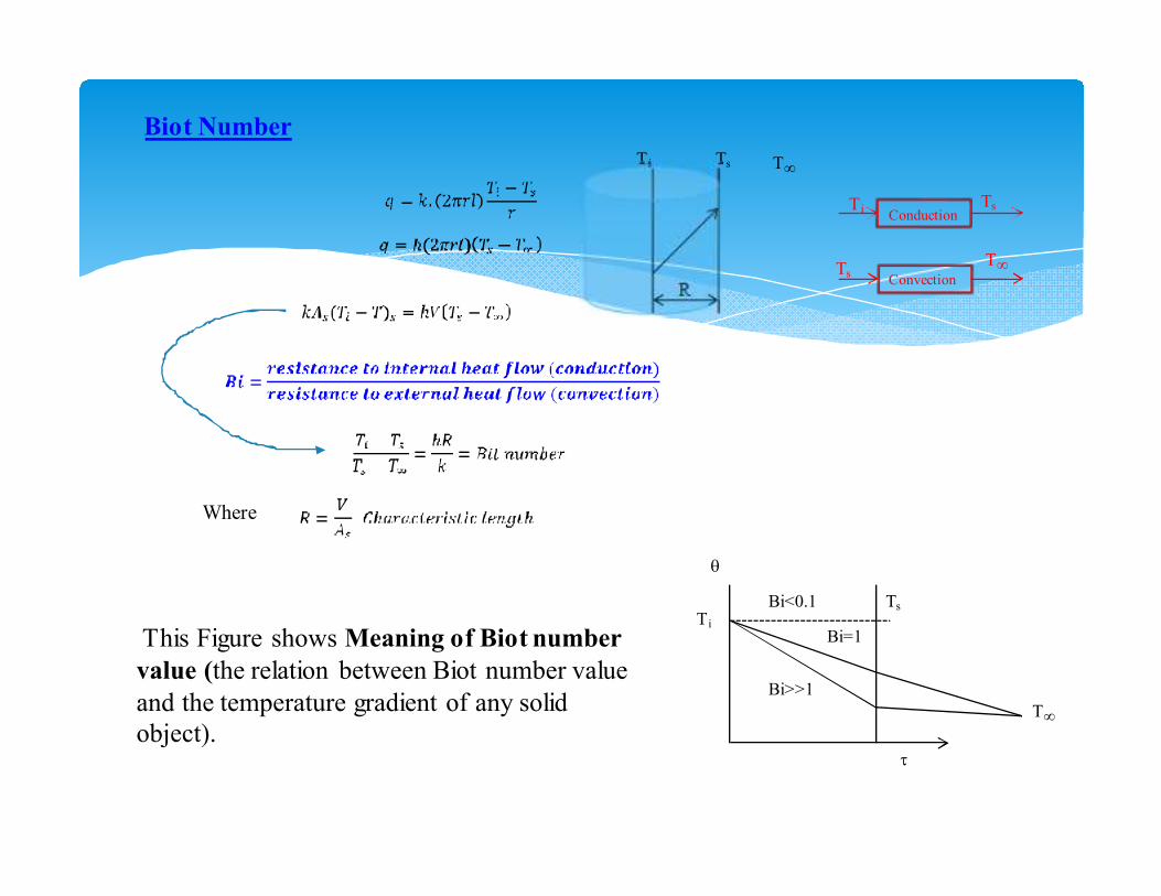
Biot Number

Where

τ

θ

T i

Ts

T∞

Bi<0.1

Bi=1

Bi>>1

This Figure shows Meaning of Biot number

value (the relation between Biot number value

and the temperature gradient of any solid

object).

ConvectionTs

T∞

ConductionT i

Ts

R

T i Ts T∞

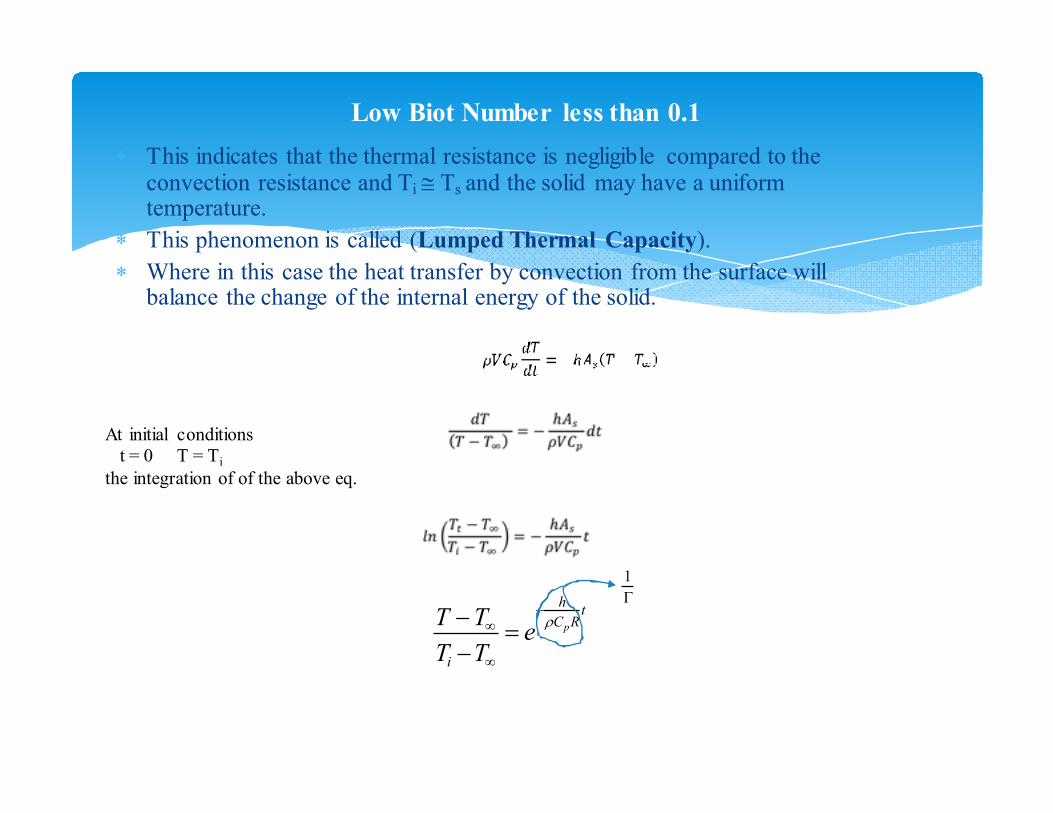
∗ This indicates that the thermal resistance is negligible compared to the convection resistance and Ti ≅ Ts and the solid may have a uniform temperature.

∗ This phenomenon is called (Lumped Thermal Capacity).

∗ Where in this case the heat transfer by convection from the surface will balance the change of the internal energy of the solid.

Low Biot Number less than 0.1

At initial conditions

t = 0 T = Ti

the integration of of the above eq.

T −T∞

Ti −T∞

= e−h

ρCpRt

1

Γ

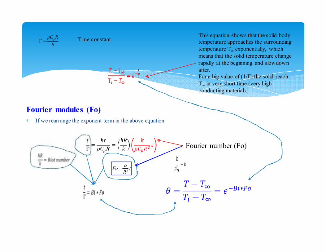
This equation shows that the solid body

temperature approaches the surrounding

temperature T∞ exponentially, which

means that the solid temperature change

rapidly at the beginning and slowdown

after.

For a big value of (1/Γ) the solid reach

T∞ in very short time (very high

conducting material).

Γ =ρCpR

hTime constant

Fourier modules (Fo)

∗ If we rearrange the exponent term in the above equation

Fourier number (Fo)

Fo =α

R2t

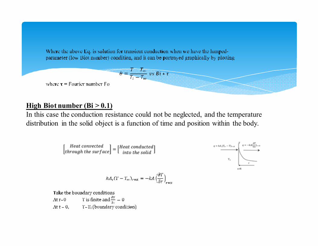
High Biot number (Bi > 0.1)

In this case the conduction resistance could not be neglected, and the temperature

distribution in the solid object is a function of time and position within the body.

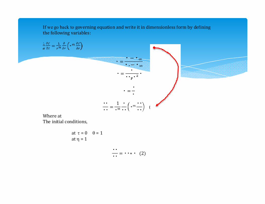
If we go back to governingequationandwriteitindimensionlessformbydefining

thefollowingvariables:

= �

� =� − �∞

��− �∞

� =�

�� ��

� =�

�

��

��=

1

�

�

�����

�� (1)

Whereat

Theinitialconditions,

atτ =0θ=1

atη=1

��

��= ��∗ � (2)

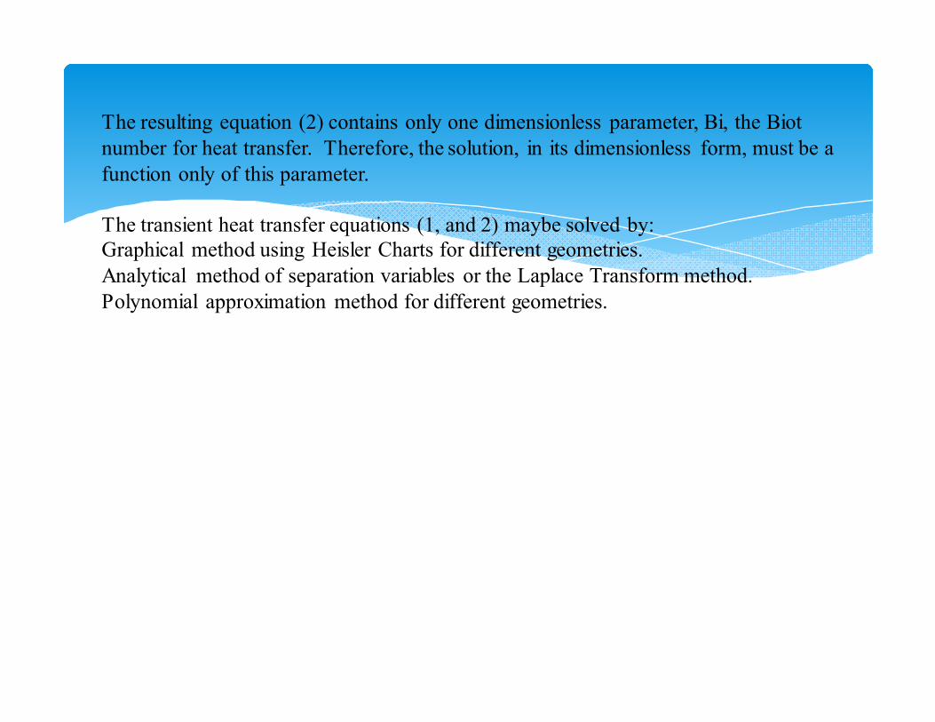
The resulting equation (2) contains only one dimensionless parameter, Bi, the Biot

number for heat transfer. Therefore, the solution, in its dimensionless form, must be a

function only of this parameter.

The transient heat transfer equations (1, and 2) maybe solved by:

Graphical method using Heisler Charts for different geometries.

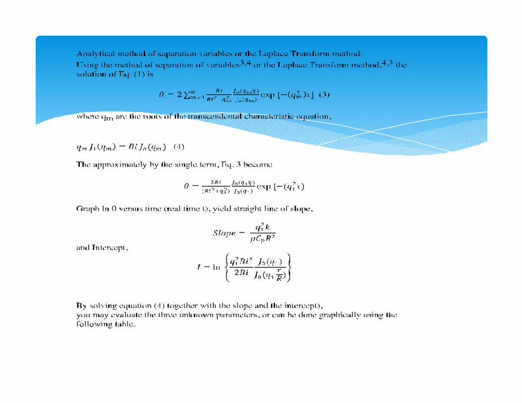
Analytical method of separation variables or the Laplace Transform method.

Polynomial approximation method for different geometries.

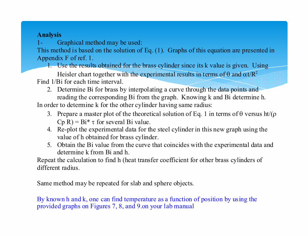
Analysis

1- Graphical method may be used:

This method is based on the solution of Eq. (1). Graphs of this equation are presented in

Appendix F of ref. 1. 1. Use the results obtained for the brass cylinder since its k value is given. Using

Heisler chart together with the experimental results in terms of θ and αt/R2 Find 1/Bi for each time interval.

2. Determine Bi for brass by interpolating a curve through the data points and

reading the corresponding Bi from the graph. Knowing k and Bi determine h.

In order to determine k for the other cylinder having same radius:

3. Prepare a master plot of the theoretical solution of Eq. 1 in terms of θ versus ht/(ρ

Cp R) = Bi* τ for several Bi value. 4. Re-plot the experimental data for the steel cylinder in this new graph using the

value of h obtained for brass cylinder.

5. Obtain the Bi value from the curve that coincides with the experimental data and determine k from Bi and h.

Repeat the calculation to find h (heat transfer coefficient for other brass cylinders of

different radius.

Same method may be repeated for slab and sphere objects.

By known h and k, one can find temperature as a function of position by using the provided graphs on Figures 7, 8, and 9.on your lab manual