Embed Size (px)
Citation preview
Unit-IV
COPLANAR NON-CONCURRENT FORCE SYSTEMS By
Prof. G. Ravi
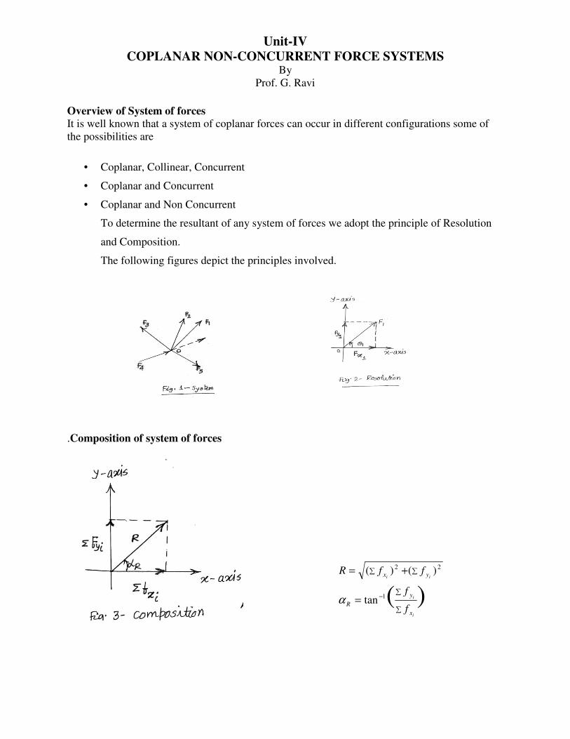
Overview of System of forces
It is well known that a system of coplanar forces can occur in different configurations some of
the possibilities are
• Coplanar, Collinear, Concurrent
• Coplanar and Concurrent
• Coplanar and Non Concurrent
To determine the resultant of any system of forces we adopt the principle of Resolution
and Composition.
The following figures depict the principles involved.
.Composition of system of forces
)(1
22
tan
)()(
i
i
ii
x
y
R
yx
f
f
ffR
∑
∑
∑∑
−=
+=
α
Equilibrium: Equilibrium is the status of the body when it is subjected to a system of forces. We
know that for a system of forces acting on a body the resultant can be determined. By Newton’s
2nd
Law of Motion the body then should move in the direction of the resultant with some
acceleration. If the resultant force is equal to zero it implies that the net effect of the system of
forces is zero this represents the state of equilibrium. For a system of coplanar concurrent forces
for the resultant to be zero, hence
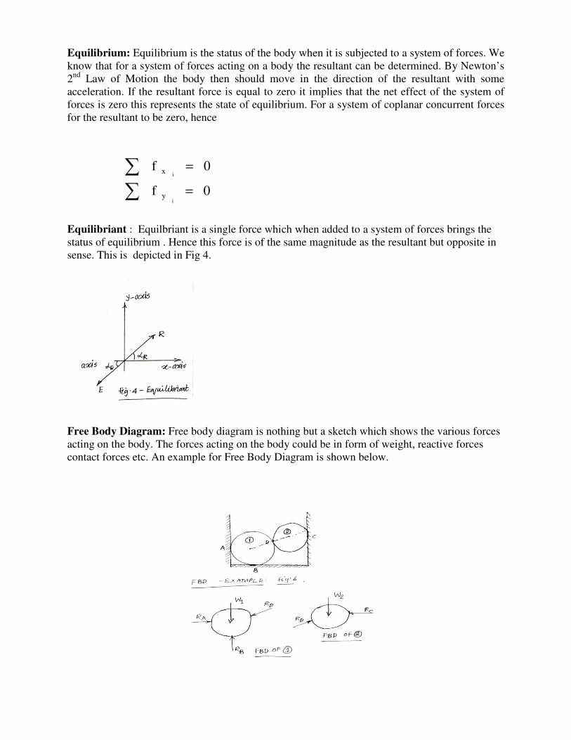
Equilibriant : Equilbriant is a single force which when added to a system of forces brings the
status of equilibrium . Hence this force is of the same magnitude as the resultant but opposite in
sense. This is depicted in Fig 4.
Free Body Diagram: Free body diagram is nothing but a sketch which shows the various forces
acting on the body. The forces acting on the body could be in form of weight, reactive forces
contact forces etc. An example for Free Body Diagram is shown below.
0f
0f
i
i
y
x
=
=
∑∑
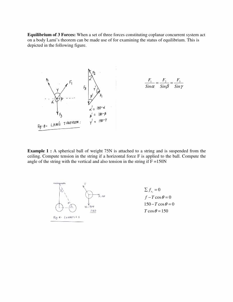
Equilibrium of 3 Forces: When a set of three forces constituting coplanar concurrent system act
on a body Lami’s theorem can be made use of for examining the status of equilibrium. This is
depicted in the following figure.
Example 1 : A spherical ball of weight 75N is attached to a string and is suspended from the
ceiling. Compute tension in the string if a horizontal force F is applied to the ball. Compute the
angle of the string with the vertical and also tension in the string if F =150N
γβα Sin
F
Sin
F
Sin
F 321 ==
150cos
0cos150
0cos
0
=
=−
=−
=∑
θ
θ
θ
T
T
Tf
fix
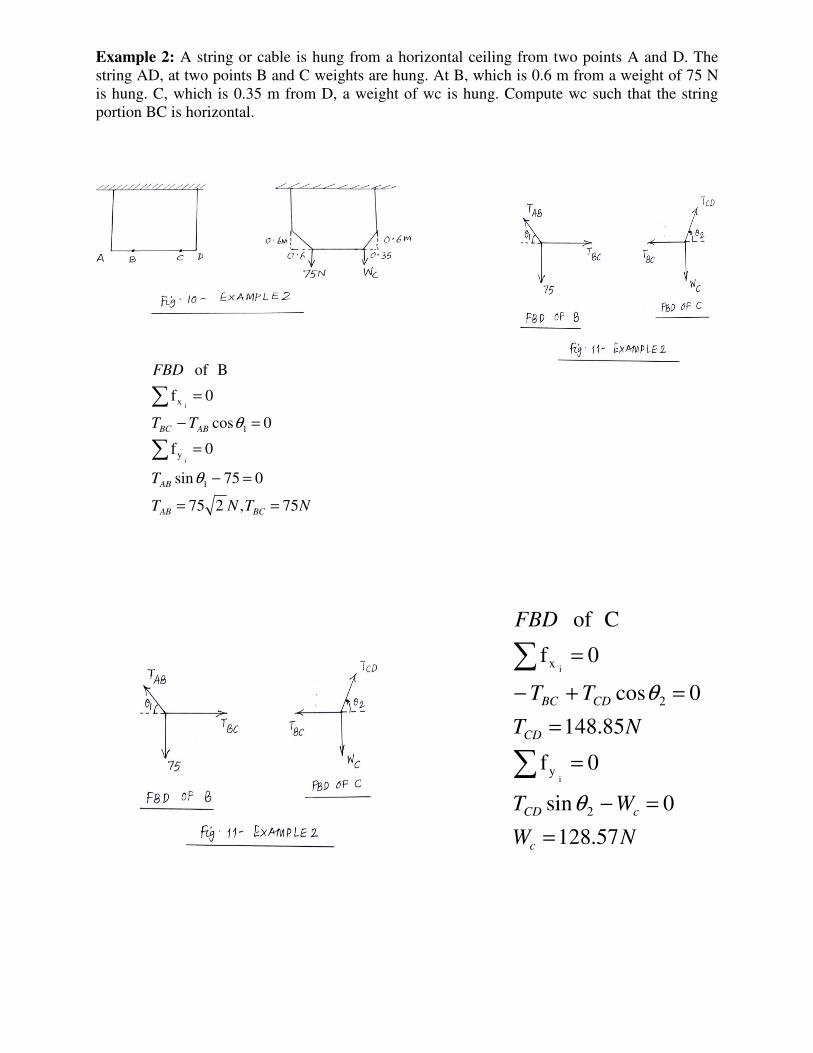
Example 2: A string or cable is hung from a horizontal ceiling from two points A and D. The
string AD, at two points B and C weights are hung. At B, which is 0.6 m from a weight of 75 N
is hung. C, which is 0.35 m from D, a weight of wc is hung. Compute wc such that the string
portion BC is horizontal.
NTNT
T
TT
FBD
BCAB
AB
ABBC
75,275
075sin
0f
0cos
0f
B of
1
y
1
x
i
i
==
=−
=
=−
=
∑
∑
θ
θ
NW
WT
NT
TT
FBD
c
cCD
CD
CDBC
57.128
0sin
0f
85.148
0cos
0f
C of
2
y
2
x
i
i
=
=−
=
=
=+−
=
∑
∑
θ
θ
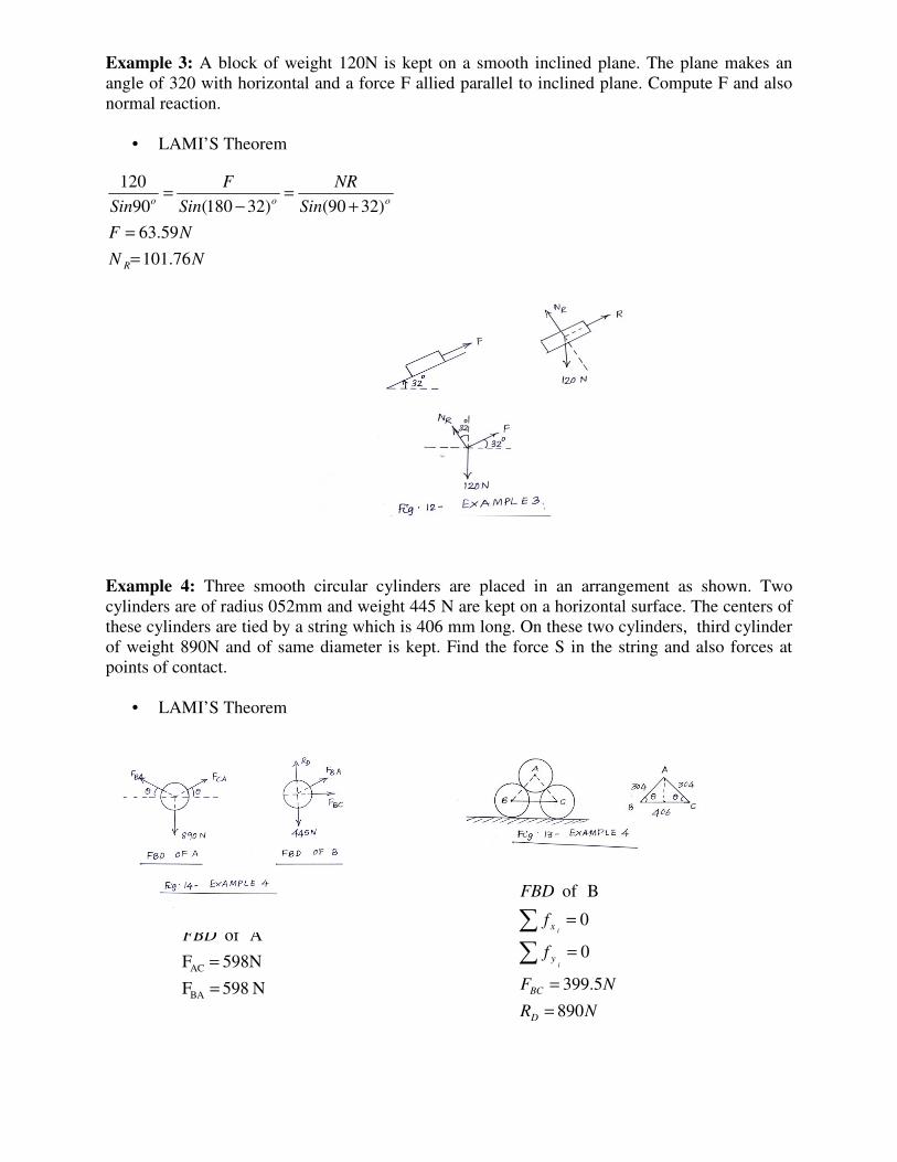
Example 3: A block of weight 120N is kept on a smooth inclined plane. The plane makes an
angle of 320 with horizontal and a force F allied parallel to inclined plane. Compute F and also
normal reaction.
• LAMI’S Theorem
Example 4: Three smooth circular cylinders are placed in an arrangement as shown. Two
cylinders are of radius 052mm and weight 445 N are kept on a horizontal surface. The centers of
these cylinders are tied by a string which is 406 mm long. On these two cylinders, third cylinder
of weight 890N and of same diameter is kept. Find the force S in the string and also forces at
points of contact.
• LAMI’S Theorem
NN
NF
Sin
NR
Sin
F
Sin
R
ooo
76.101
59.63
)3290()32180(90
120
=
=
+=
−=
N 598 F
598N F
A of
BA
AC
=
=
FBD
NR
NF
f
f
FBD
D
BC
y
x
i
i
890
5.399
0
0
B of
=
=
=
=
∑∑
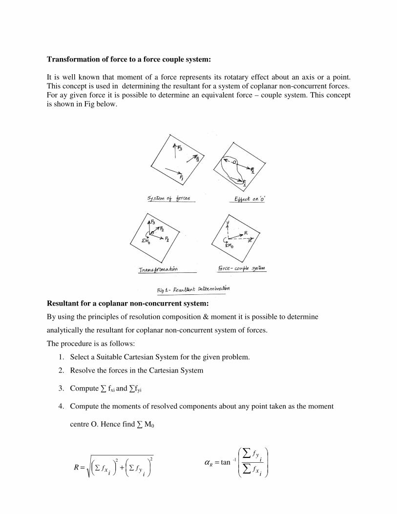
Transformation of force to a force couple system:
It is well known that moment of a force represents its rotatary effect about an axis or a point.
This concept is used in determining the resultant for a system of coplanar non-concurrent forces.
For ay given force it is possible to determine an equivalent force – couple system. This concept
is shown in Fig below.
Resultant for a coplanar non-concurrent system:
By using the principles of resolution composition & moment it is possible to determine
analytically the resultant for coplanar non-concurrent system of forces.
The procedure is as follows:
1. Select a Suitable Cartesian System for the given problem.
2. Resolve the forces in the Cartesian System
3. Compute ∑ fxi and ∑fyi
4. Compute the moments of resolved components about any point taken as the moment
centre O. Hence find ∑ M0
22
+
= ∑∑
iyf
ixfR
=
∑
∑
ixf
iyf
R tan 1-α

5. Compute moment arm
6. Also compute x- intercept as
7. And Y intercept as
Example 1: Compute the resultant for the system of forces shown in Fig 2 and hence compute
the Equilibriant.
R
Md
o
R
∑=
∑∑
=ix
o
Rf
MX
∑∑
=ix
o
Rf
My
KN 28.8
60 cos 32 - 44.8 o
=
=∑ ixf
KNM
M
f
oo
o
yi
34.62
)3(60sin32)4(60cos32)3(4.14
49.83
KN 44.6 R
KN 34.11 -
60sin 32- 14.4 - 8
o
R
o
−=
−+−=+
=
=
=
=
∑
∑
ς
α
m 164.28.28
34.62y
m 827.1 11.34
34.62 x
m 396.1 64.44
34.62d
R
R
R
==
==
==

Example 2: Find the Equilibriant for the rigid bar shown in Fig 3 when it is subjected to forces.
• Resultant and Equilibriant
Equilibrium: The concept of equilibrium is the same as explained earlier. For a system of
Coplanar Non concurrent forces for the status of equilibrium the equations to be satisfied are
The above principles are used in solving the following examples.
;90
516
0
o
R
y
x
KNf
f
i
i
=
−=
=
∑∑
α
KNM 1462-
)4(344)2(172)1(430
=
−+−=+∑ AMς
;0 ;0 ;0 === ∑∑∑ oyx Mffii
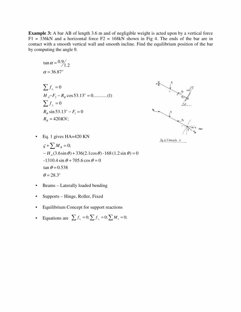
Example 3: A bar AB of length 3.6 m and of negligible weight is acted upon by a vertical force
F1 = 336kN and a horizontal force F2 = 168kN shown in Fig 4. The ends of the bar are in
contact with a smooth vertical wall and smooth incline. Find the equilibrium position of the bar
by computing the angle θ.
• Eq. 1 gives HA=420 KN
• Beams – Laterally loaded bending
• Supports – Hinge, Roller, Fixed
• Equilibrium Concept for support reactions
• Equations are
o87.36
2.19.0tan
=
=
α
α
;420
013.53sin
0
)1..(..........013.53cos
0
1
2
KNR
FR
f
RFH
f
B
o
B
y
o
BA
x
i
i
=
=−
=
=−−
=
∑
∑
o
A
B
H
M
3.28
0.538 tan
0 cos 705.6 sin 1310.4-
0)sin (1.2 168 -)cos1.2(336)sin6.3(
;0
=
=
=+
=+−
=+∑
θ
θ
θθ
θθθ
ς
;0 ;0 ;0 === ∑∑∑ oyx Mffii
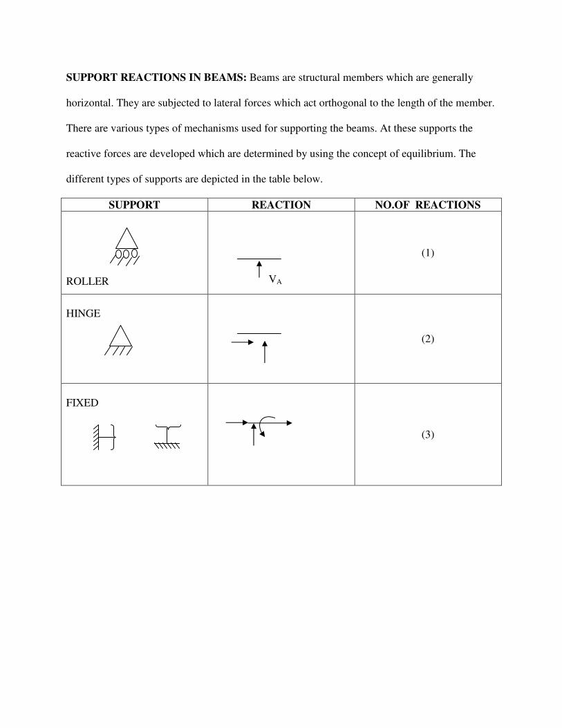
SUPPORT REACTIONS IN BEAMS: Beams are structural members which are generally
horizontal. They are subjected to lateral forces which act orthogonal to the length of the member.
There are various types of mechanisms used for supporting the beams. At these supports the
reactive forces are developed which are determined by using the concept of equilibrium. The
different types of supports are depicted in the table below.
SUPPORT REACTION NO.OF REACTIONS
ROLLER
(1)
HINGE
(2)
FIXED
(3)
VA
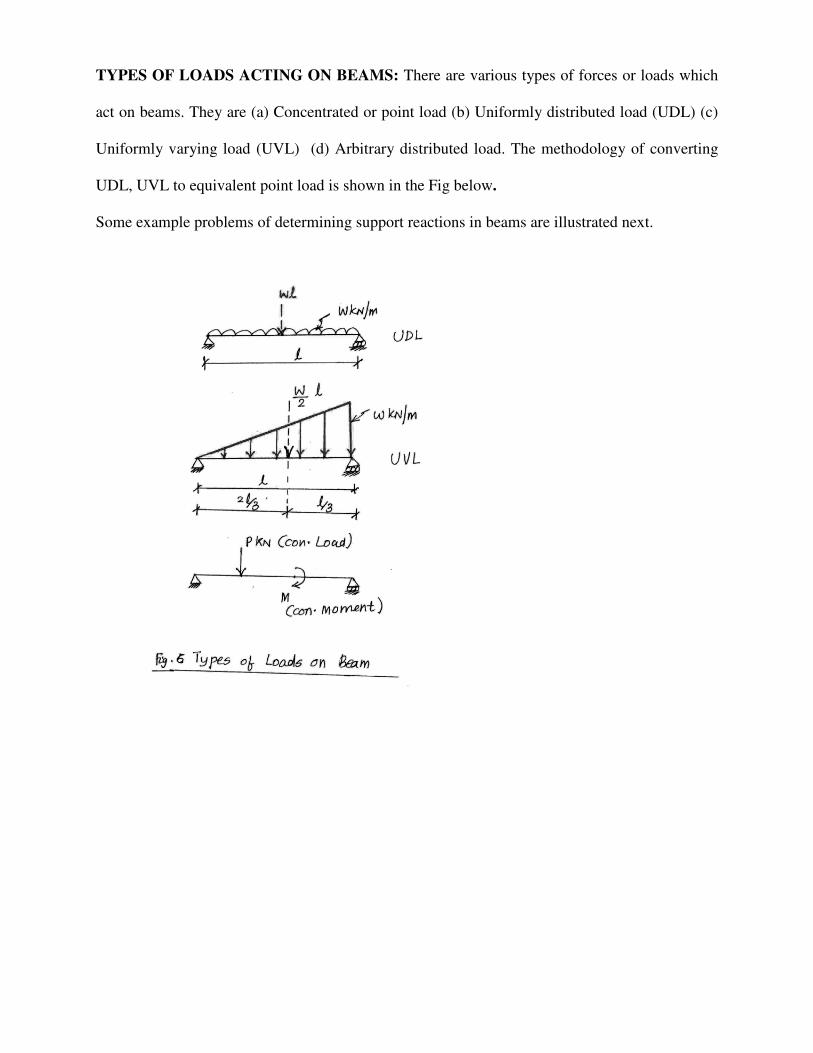
TYPES OF LOADS ACTING ON BEAMS: There are various types of forces or loads which
act on beams. They are (a) Concentrated or point load (b) Uniformly distributed load (UDL) (c)
Uniformly varying load (UVL) (d) Arbitrary distributed load. The methodology of converting
UDL, UVL to equivalent point load is shown in the Fig below.
Some example problems of determining support reactions in beams are illustrated next.
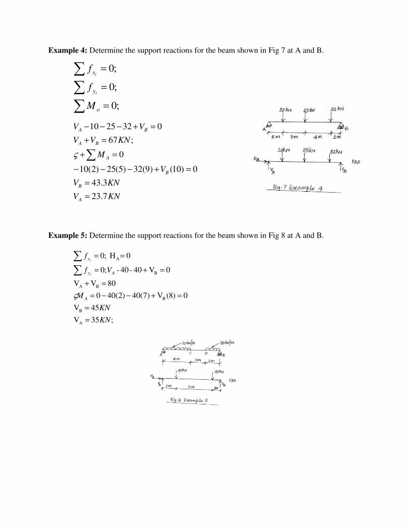
Example 4: Determine the support reactions for the beam shown in Fig 7 at A and B.
Example 5: Determine the support reactions for the beam shown in Fig 8 at A and B.
;0
;0
;0
=
=
=
∑∑∑
o
y
x
M
f
f
i
i
KNV
KNV
V
M
KNVV
VV
A
B
B
A
BA
BA
7.23
3.43
0)10()9(32)5(25)2(10
0
;67
0322510
=
=
=+−−−
=+
=+
=+−−−
∑ς
;35V
45V
0)8(V)7(40)2(400
80VV
0V40-40-;0
0H ;0
A
B
B
BA
B
A
KN
KN
M
Vf
f
A
Ay
x
i
i
=
=
=+−−=
=+
=+=
==
∑∑
ς
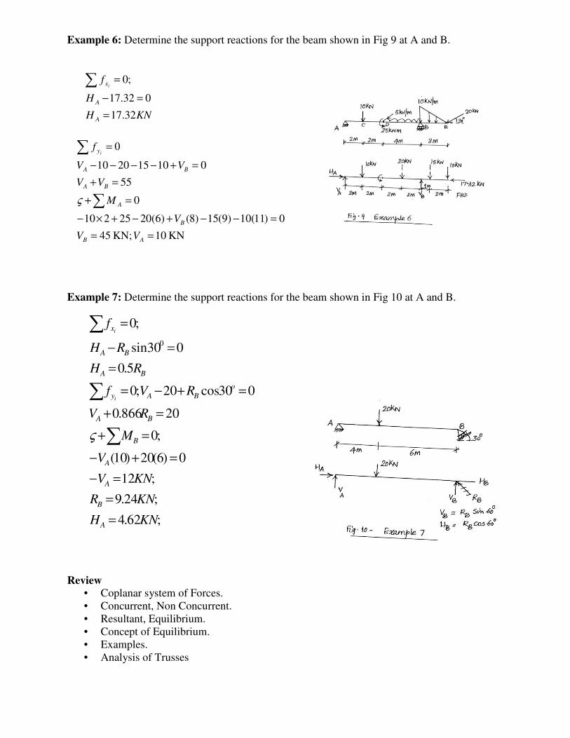
Example 6: Determine the support reactions for the beam shown in Fig 9 at A and B.
Example 7: Determine the support reactions for the beam shown in Fig 10 at A and B.
Review
• Coplanar system of Forces.
• Concurrent, Non Concurrent.
• Resultant, Equilibrium.
• Concept of Equilibrium.
• Examples.
• Analysis of Trusses
KNH
H
f
A
A
xi
32.17
032.17
;0
=
=−
=∑
KN 10 KN; 45
0)11(10)9(15)8()6(2025210
0
55
010152010
0
==
=−−+−+×−
=+
=+
=+−−−−
=
∑
∑
AB
B
A
BA
BA
y
VV
V
M
VV
VV
fi
ς
;62.4
;24.9
;12
0)6(20)10(
;0
20866.0
030cos20;0
5.0
030sin
;0
0
KNH
KNR
KNV
V
M
RV
RVf
RH
RH
f
A
B
A
A
B
BA
o
BAy
BA
BA
x
i
i
=
=
=−
=+−
=+
=+
=+−=
=
=−
=
∑
∑
∑
ς
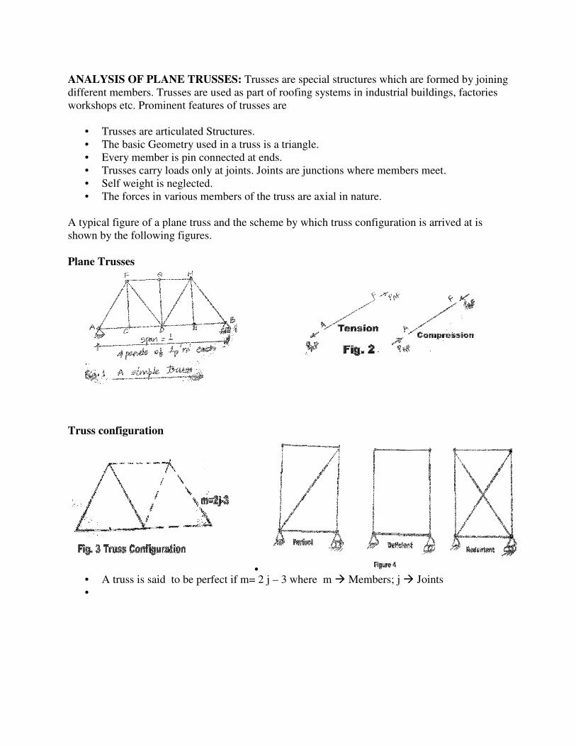
ANALYSIS OF PLANE TRUSSES: Trusses are special structures which are formed by joining
different members. Trusses are used as part of roofing systems in industrial buildings, factories
workshops etc. Prominent features of trusses are
• Trusses are articulated Structures.
• The basic Geometry used in a truss is a triangle.
• Every member is pin connected at ends.
• Trusses carry loads only at joints. Joints are junctions where members meet.
• Self weight is neglected.
• The forces in various members of the truss are axial in nature.
A typical figure of a plane truss and the scheme by which truss configuration is arrived at is
shown by the following figures.
Plane Trusses
Truss configuration
• • A truss is said to be perfect if m= 2 j – 3 where m � Members; j � Joints
•
Analysis of Trusses: Analysis of trusses would imply determining forces in various members.
These forces will be in the form of Axial Tension (or) Compression. The
Equilibrium concept is made use of for analyzing the trusses. The two methods of analysis are
1. Method of Joints.
2. Method of Sections.
These two methods of analysis are illustrated by the following examples
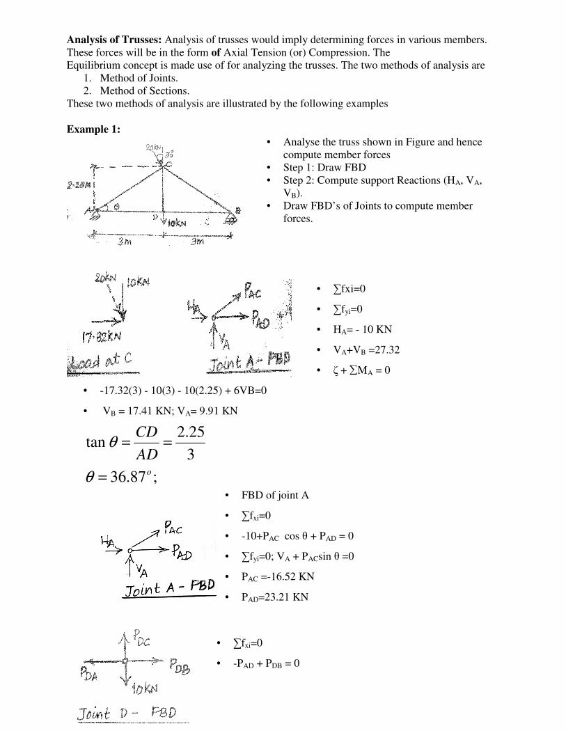
Example 1: • Analyse the truss shown in Figure and hence
compute member forces
• Step 1: Draw FBD
• Step 2: Compute support Reactions (HA, VA,
VB).
• Draw FBD’s of Joints to compute member
forces.
• ∑fxi=0
• ∑fyi=0
• HA= - 10 KN
• VA+VB =27.32
• ζ + ∑MA = 0
• -17.32(3) - 10(3) - 10(2.25) + 6VB=0
• VB = 17.41 KN; VA= 9.91 KN
• FBD of joint A
• ∑fxi=0
• -10+PAC cos θ + PAD = 0
• ∑fyi=0; VA + PACsin θ =0
• PAC =-16.52 KN
• PAD=23.21 KN
• ∑fxi=0
• -PAD + PDB = 0
;87.36
3
25.2 tan
o
AD
CD
=
==
θ
θ

• PDB = 23.21 KN
• ∑fyi=0
• -10+PCD = 0
• PCD = 10 KN
• ∑fxi=0
• -PBD – PBC cos θ =0
• PBC = -29.02 KN
• ∑fyi=0
• VB +PBC sin θ = 0
• 17.41 – 29.02 sin θ = 0
•
Sl.No Member Force Nature
1 AC 16.52 C
2 AD 23.21 T
3 CB 29.02 C
4 CD 10 T
5 DB 23.21 T
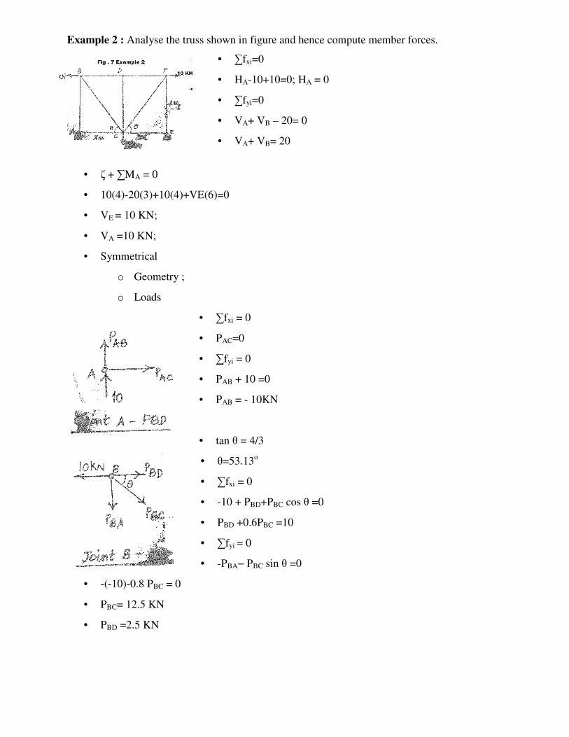
Example 2 : Analyse the truss shown in figure and hence compute member forces.
• ∑fxi=0
• HA-10+10=0; HA = 0
• ∑fyi=0
• VA+ VB – 20= 0
• VA+ VB= 20
• ζ + ∑MA = 0
• 10(4)-20(3)+10(4)+VE(6)=0
• VE = 10 KN;
• VA =10 KN;
• Symmetrical
o Geometry ;
o Loads
• ∑fxi = 0
• PAC=0
• ∑fyi = 0
• PAB + 10 =0
• PAB = - 10KN
• tan θ = 4/3
• θ=53.13o
• ∑fxi = 0
• -10 + PBD+PBC cos θ =0
• PBD +0.6PBC =10
• ∑fyi = 0
• -PBA− PBC sin θ =0
• -(-10)-0.8 PBC = 0
• PBC= 12.5 KN
• PBD =2.5 KN
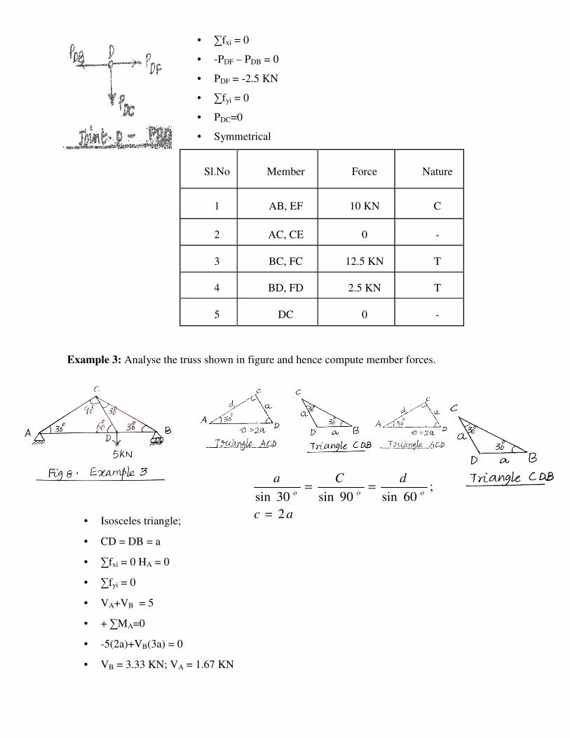
• ∑fxi = 0
• -PDF – PDB = 0
• PDF = -2.5 KN
• ∑fyi = 0
• PDC=0
• Symmetrical
Sl.No Member Force Nature
1 AB, EF 10 KN C
2 AC, CE 0 -
3 BC, FC 12.5 KN T
4 BD, FD 2.5 KN T
5 DC 0 -
Example 3: Analyse the truss shown in figure and hence compute member forces.
• Isosceles triangle;
• CD = DB = a
• ∑fxi = 0 HA = 0
• ∑fyi = 0
• VA+VB = 5
• + ∑MA=0
• -5(2a)+VB(3a) = 0
• VB = 3.33 KN; VA = 1.67 KN
ac
dCaooo
2
;60sin90sin30sin
=
==
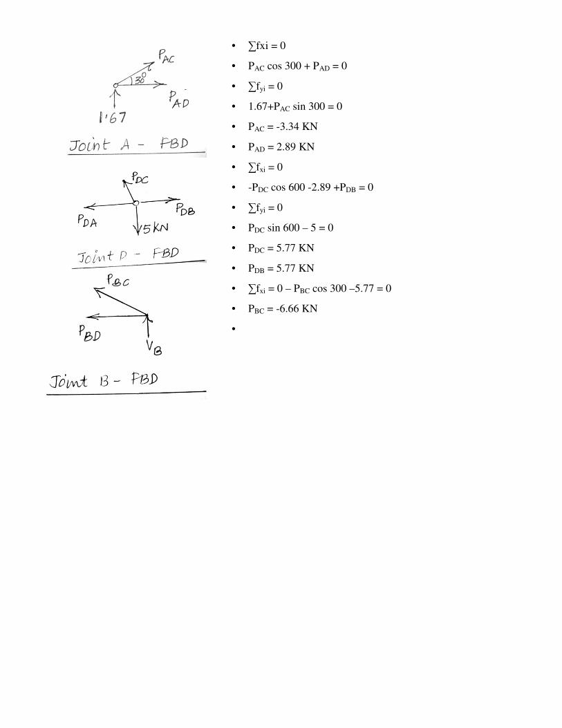
• ∑fxi = 0
• PAC cos 300 + PAD = 0
• ∑fyi = 0
• 1.67+PAC sin 300 = 0
• PAC = -3.34 KN
• PAD = 2.89 KN
• ∑fxi = 0
• -PDC cos 600 -2.89 +PDB = 0
• ∑fyi = 0
• PDC sin 600 – 5 = 0
• PDC = 5.77 KN
• PDB = 5.77 KN
• ∑fxi = 0 – PBC cos 300 –5.77 = 0
• PBC = -6.66 KN
•
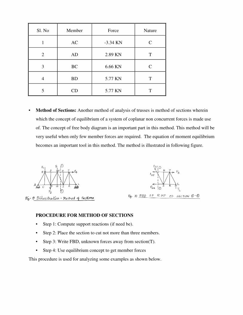
Sl. No Member Force Nature
1 AC -3.34 KN C
2 AD 2.89 KN T
3 BC 6.66 KN C
4 BD 5.77 KN T
5 CD 5.77 KN T
• Method of Sections: Another method of analysis of trusses is method of sections wherein
which the concept of equilibrium of a system of coplanar non concurrent forces is made use
of. The concept of free body diagram is an important part in this method. This method will be
very useful when only few member forces are required. The equation of moment equilibrium
becomes an important tool in this method. The method is illustrated in following figure.
PROCEDURE FOR METHOD OF SECTIONS
• Step 1: Compute support reactions (if need be).
• Step 2: Place the section to cut not more than three members.
• Step 3: Write FBD, unknown forces away from section(T).
• Step 4: Use equilibrium concept to get member forces
This procedure is used for analyzing some examples as shown below.
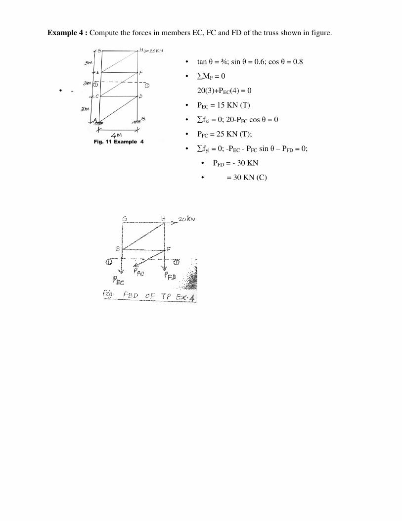
Example 4 : Compute the forces in members EC, FC and FD of the truss shown in figure.
• tan θ = ¾; sin θ = 0.6; cos θ = 0.8
• ∑MF = 0
• - 20(3)+PEC(4) = 0
• PEC = 15 KN (T)
• ∑fxi = 0; 20-PFC cos θ = 0
• PFC = 25 KN (T);
• ∑fyi = 0; -PEC - PFC sin θ – PFD = 0;
• PFD = - 30 KN
• = 30 KN (C)
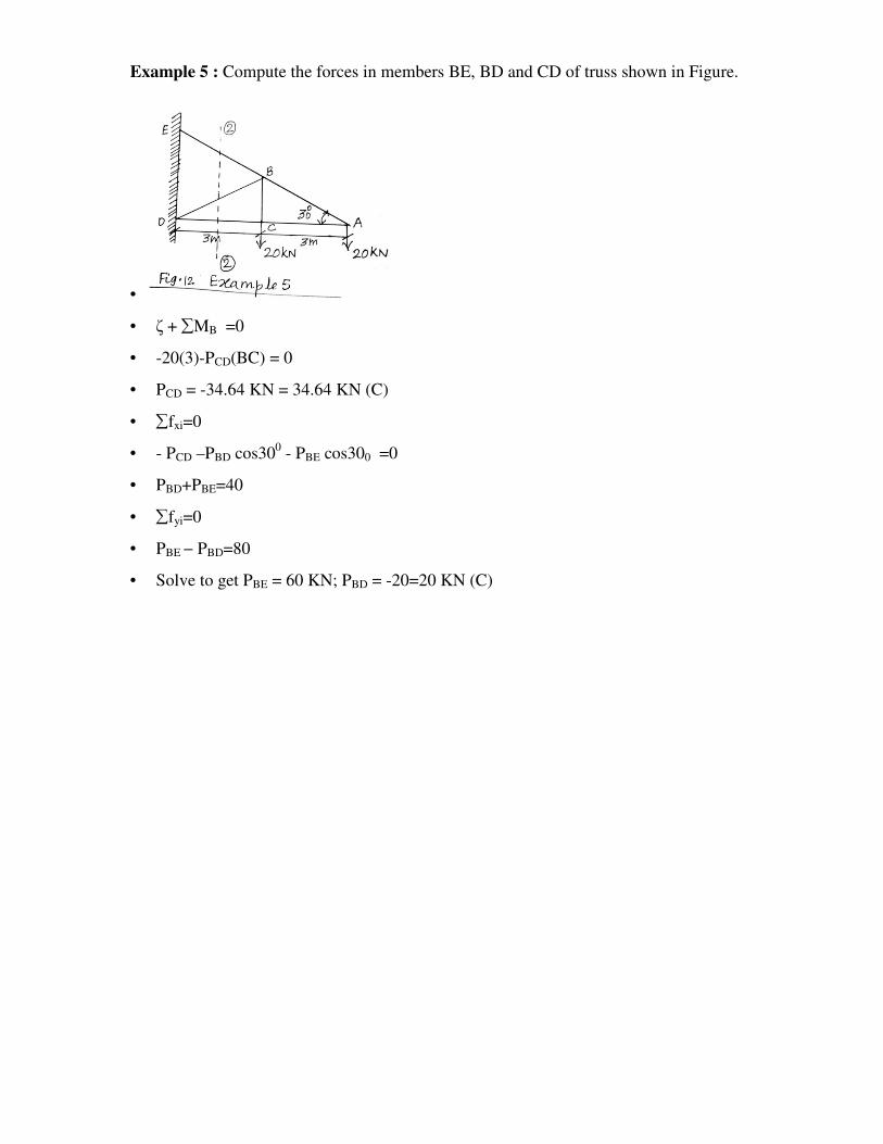
Example 5 : Compute the forces in members BE, BD and CD of truss shown in Figure.
•
• ζ + ∑MB =0
• -20(3)-PCD(BC) = 0
• PCD = -34.64 KN = 34.64 KN (C)
• ∑fxi=0
• - PCD –PBD cos300 - PBE cos300 =0
• PBD+PBE=40
• ∑fyi=0
• PBE − PBD=80
• Solve to get PBE = 60 KN; PBD = -20=20 KN (C)
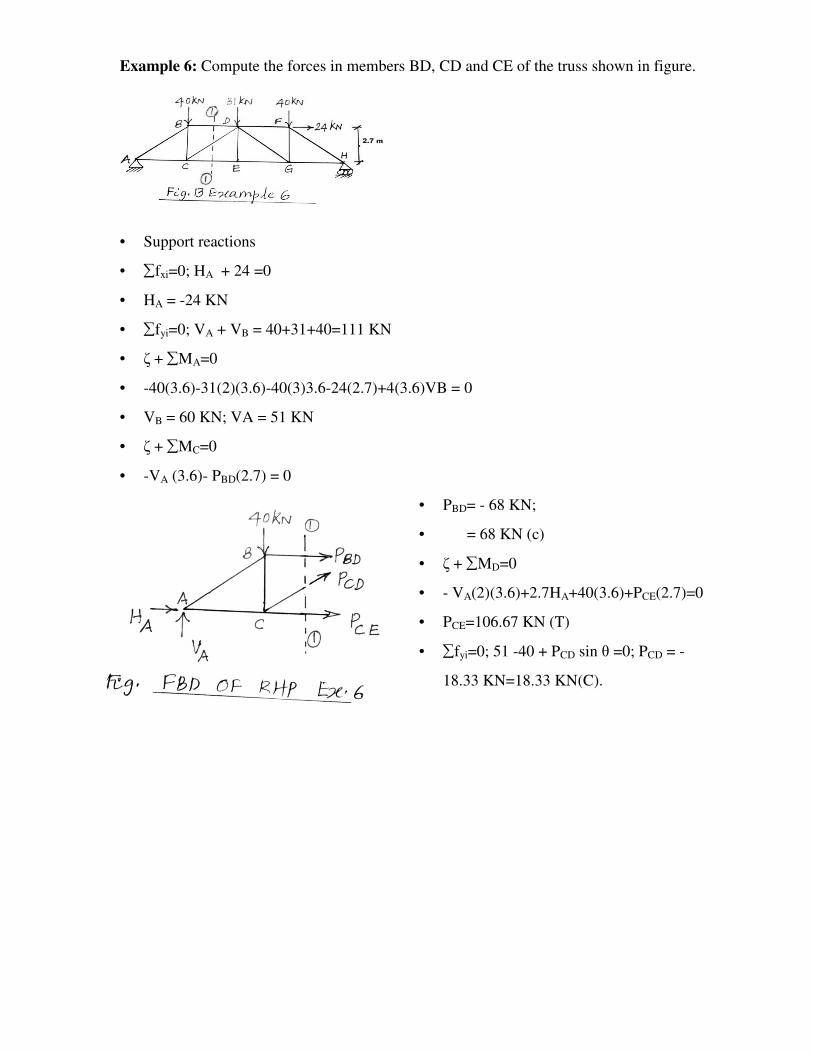
Example 6: Compute the forces in members BD, CD and CE of the truss shown in figure.
• Support reactions
• ∑fxi=0; HA + 24 =0
• HA = -24 KN
• ∑fyi=0; VA + VB = 40+31+40=111 KN
• ζ + ∑MA=0
• -40(3.6)-31(2)(3.6)-40(3)3.6-24(2.7)+4(3.6)VB = 0
• VB = 60 KN; VA = 51 KN
• ζ + ∑MC=0
• -VA (3.6)- PBD(2.7) = 0
• PBD= - 68 KN;
• = 68 KN (c)
• ζ + ∑MD=0
• - VA(2)(3.6)+2.7HA+40(3.6)+PCE(2.7)=0
• PCE=106.67 KN (T)
• ∑fyi=0; 51 -40 + PCD sin θ =0; PCD = -
18.33 KN=18.33 KN(C).