Unit - 1

Force Analysis and flywheels

Introduction

A machine is a device that performs work and, as such, transmits energy by means mechanical force from a

power source to a driven load. It is necessary in the design machine mechanisms to know the manner in which

forces are transmitted from input to the output, so that the components of the machine can be properly size withstand

the stresses that are developed. If the members are not designed to strong enough, then failure will occur during

machine operation; if, on the other hand, the machine is over designed to have much more strength than required,

then the machine may not be competitive with others in terms of cost, weight, size, power requirements, or other

criteria. The bucket load and static weight loads may far exceed any dynamic loads due to accelerating masses, and a

static-force analysis would be justified. An analysis that includes inertia effects is called a dynamic-force analysis

and will be discussed in the next chapter. An example of an application where a dynamic-force analysis would be

required is in the design of an automatic sewing machine, where, due to high operating speeds, the inertia forces

may be greater than the external loads on the machine.

Another assumption deals with the rigidity of the machine components. No material is truly rigid, and all

materials will experience significant deformation if the forces, either external or inertial in nature, are great enough.

It will be assumed in this chapter and the next that deformations are so small as to be negligible and, therefore, the

members will be treated as though they are rigid. The subject of mechanical vibrations, which is beyond the scope of

this book, considers the flexibility of machine components and the resulting effects on machine behavior. A third

major assumption that is often made is that friction effects are negligible. Friction is inherent in all devices, and its

degree is dependent upon many factors, including types of bearings, lubrication, loads, environmental conditions,

and so on. Friction will be neglected in the first few sections of this chapter, with an introduction to the subject

presented. In addition to assumptions of the types discussed above, other assumptions may be necessary, and some

of these will be addressed at various points throughout the chapter.

The first part of this chapter is a review of general force analysis principles and will also establish some of

the convention and terminology to be used in succeeding sections. The remainder of the chapter will then present

both graphical and analytical methods for static-force analysis of machines.

Free-Body Diagrams:

Engineering experience has demonstrated the importance and usefulness of free-body diagrams in force

analysis. A free-body diagram is a sketch or drawing of part or all of a system, isolated in order to determine the

nature of forces acting on that body. Sometimes a free-body diagram may take the form of a mental picture;

however, actual sketches are strongly recommended, especially for complex mechanical systems.

Generally, the first, and one of the most important, steps in a successful force analysis is the identification

of the free bodies to be used. Figures 1.1B through 1.1E show examples of various free bodies that might be

Figure1.1(A) A four-bar linkage.

considered in the analysis of the four-bar linkage shown in Figure 5.1A. In Figure 5.1B, the free body consists of the

three moving members isolated from the frame; here, the forces acting on the free body include a driving force or

torque, external loads, and the forces transmitted:

Static Equilibrium:

For a free body in static equilibrium, the vector sum of all forces acting on the body must be zero and the

vector sum of all moments about any arbitrary point must also be zero. These conditions can be expressed

mathematically as follows:

0F (1.1A)

0T (1.1B)

Figure 1.1(B) Free-body diagram of thethree moving links

Figure 1.1(C) Free-body diagram of twoconnected links

Figure 1.1(D) Free-body diagram of asingle link

Figure 1.1(E) Free body diagram of partof a link.

F03 F03

Since each of these vector equations represents three scalar equations, there are a total of six independent scalar

conditions that must be satisfied for the general case of equilibrium under three-dimensional loading.

There are many situations where the loading is essentially planar; in which case, forces can be described by

two-dimensional vectors. If the xy plane designates the plane of loading, then the applicable form of Eqs. 1.1A and

1.1B is:-

0xF (1.2A)

0yF (1.2B)

0zT (1.2C)Eqs. 1.2A to 1.2C are three scalar equations that state that, for the case of two-dimensional xy loading, the

summations of forces in the x and y directions must individually equal zero and the summation of moments about

any arbitrary point in the plane must also equal zero. The remainder of this chapter deals with two-dimensional force

analysis. A common example of three-dimensional forces is gear forces.

Superposition:

The principle of superposition of forces is an extremely useful concept, particularly in graphical force

analysis. Basically, the principle states that, for linear systems, the net effect of multiple loads on a system is equal

to the superposition (i.e., vector summation) of the effects of the individual loads considered one at a time.

Physically, linearity refers to a direct proportionality between input force and output force. Its mathematical

characteristics will be discussed in the section on analytical force analysis. Generally, in the absence of Coulomb or

dry friction, most mechanisms are linear for force analysis purposes, despite the fact that many of these mechanisms

exhibit very nonlinear motions. Examples and further discussion in later sections will demonstrate the application of

this principle

Graphical Force Analysis:

Graphical force analysis employs scaled free-body diagrams and vector graphics in the determination of

unknown machine forces. The graphical approach is best suited for planar force systems. Since forces are normally

not constant during machine motion. analyses may be required for a number of mechanism positions; however, in

many cases, critical maximum-force positions can be identified and graphical analyses performed for these positions

only. An important advantage of the graphical approach is that it provides useful insight as to the nature of the forces

in the physical system.

This approach suffers from disadvantages related to accuracy and time. As is true of any graphical

procedure, the results are susceptible to drawing and measurement errors. Further, a great amount of graphics time

and effort can be expended in the iterative design of a machine mechanism for which fairly thorough knowledge of

force-time relationships is required. In recent years, the physical insight of the graphics approach and the speed and

accuracy inherent in the computer-based analytical approach have been brought together through computer graphics

systems, which have proven to be very effective engineering design tools. There are a few special types of member

loadings that are repeatedly encountered in the force analysis of mechanisms, These include a member subjected to

two forces, a member subjected to three forces, and a member subjected to two forces and a couple. These special

cases will be considered in the following paragraphs, before proceeding to the graphical analysis of complete

mechanisms.

Analysis of a Two-Force Member:

A member subjected to two forces is in equilibrium if and only if the two forces (1) have the samemagnitude, (2) act along the same line, and (3) are opposite in sense. Figure 1.2A shows a free-body diagram of amember acted upon by forces 1F and 2F where the points of application of these forces are points A and B. For

equilibrium the directions of 1F and 2F must be along line AB and 1F must equal 2F graphical vector addition of

forces 1F and 2F is shown in Figure 1.2B, and, obviously, the resultant net force on the member is zero

when 1 2F F . The resultant moment about any point will also be zero.

Thus, if the load application points for a two-force member are known, the line of action of the forces is

defined, and it the magnitude and sense of one of the forces are known, then the other force can immediately be

determined. Such a member will either be in tension or compression.

Analysis of a Three-Force Member:

A member subjected to three forces is in equilibrium if and only if (1) the resultant of the three forces is zero,

and (2) the lines of action of the forces all intersect at the same point. The first condition guarantees equilibrium of

forces, while the second condition guarantees equilibrium of moments. The second condition can be under-stood by

considering the case when it is not satisfied. See Figure 1.3A. If moments are summed about point P, the

intersection of forces 1F and 2F , then the moments of these forces will be zero, but 3F will produce a nonzero

moment, resulting in a nonzero net moment on the member. On the other hand, if the line of action of force 3F also

passes through point P (Figure 5.3B), the net moment will be zero. This common point of intersection of the three

forces is called the point of concurrency.

A typical situation encountered is that when one of the forces, 1F , is known

completely, magnitude and direction, a second force, 2F , has known direction but

unknown magnitude, and force 3F has unknown magnitude and direction. The graphical solution of this case is

depicted in Figures 1.4A through 1.4C. First, the

Figure 1.2(A) A two-force member. The resultantforce and the resultant moment both equal Zero. Figure 1.2(B) Force summation for a two-

force member

free-body diagram is drawn to a convenient scale and the points of application of the

three forces are identified. These are points A, B, and C. Next, the known force 1F is

drawn on the diagram with the proper direction and a suitable magnitude scale. The

direction of force 2F is then drawn, and the intersection of this line with an extension

of the line of action of force 1F is the concurrency point P. For equilibrium, the line

of action of force 3F must pass through points C and P and is therefore as shown in

Figure 1.4A.The force equilibrium condition states that

1 2 3 0F F F

Since the directions of all three forces are now known and the magnitude of 1F were given, this equation can be

solved for the remaining two magnitudes. A graphicalSolution follows from the fact that the three forces must form a closed vector loop, called a force polygon. The

procedure is shown in Figure 1.4B. Vector 1F is redrawn. From the head of this vector, a line is drawn in the

direction of force 2F , and from the tail, a line is drawn parallel to 3F . The intersection of these lines closes the

vector loop and determines the magnitudes of forces 2F and 3F . Note that the same solution is obtained if, instead, a

line parallel to 3F is drawn from the head of 1F , and a line parallel to 2F is drawn from the tail of 1F . See Figure

1.4C.

Figure 1.3(A) The three forces on themember do not intersect at a common pointand there is a nonzero resultant moment.

Figure 1.3(B) The three forces intersect atthe same point P, called the concurrencypoint, and the net moment is zero.

Figure 1.4(A) Graphical force analysis ofa three- force member.

Concurrency point P

Line of action of F3

Line of action F2

This is so because vector addition is commutative, and, therefore, both force polygons are equivalent to the

vector equation above. It is important to remember that, by the definition of vector addition, the force polygon

corresponding to the general force equation

0F Will have adjacent vectors connected head to tail. This principle is used in identifying

the sense of forces 2F and 3F in Figures 5.4B and 5.4C. Also, if the lines of action of 1F and 2F are parallel," then

the point of concurrency is at infinity, and the third force 3F must be parallel to the other two. In this case, the force

polygon collapses to a straight line.

Graphical Force Analysis of the Slider Crank Mechanism:

The slider crank mechanism finds extensive application in reciprocating compressors, piston engines,

presses, toggle devices, and other machines where force characteristics are important. The force analysis of this

mechanism employs most of the principles described in previous sections, as demonstrated by the following

example.

PROBLEM 1

Static-force analysis of a slider crank mechanism is discussed. Consider the slider crank linkage shown in Figure

1.5A, representing a compressor, which is operating at so low a speed that inertia effects are negligible. It is also

assumed that gravityforces are small compared with other forces and that all forces lie in the same plane.The

dimensions are OB = 30 mm and BC == 70 mm, we wish to find the required

crankshaft torque T and the bearing forces for a total gas pressure force P = 40N at the instant when the crank

angle 45 .

SOLUTIONThe graphical analysis is shown in Figure 1.5B. First, consider connecting rod 2. In the absence of gravity and

inertia forces, this link is acted on by two forces only, at pins B and C. These pins are assumed to be frictionless and,

Figure 1.4(B) Force polygon for the threeforces member.

Figure 1.4(C) An equivalent force polygonfor the three force member

OB = 30 mmBC = 70 mm

45 Figure 1.5(A) Graphical force analysis ofa slider crank mechanism, which isacted on by piston force P and cranktorque T

therefore, transmit no torque. Thus, link 2 is a two-force member loaded at each end as shown. The forces 12F and

32F lie along the link, producing zero net moment, and must be equal and opposite for equilibrium of the link. At

this point, the magnitude and sense of these forces are unknown.Next, examine piston 3, which is a three-force member. The pressure force P is completely known and is

assumed to act through the center of the piston (i.e., the pressure distribution on the piston face is assumed to besymmetric). From Newton's third law, which states that for every action there is an equal and opposite reaction, it

follows that 23 32F F , and the direction of 23F is therefore known. In the absence of friction, the force of the

cylinder on the piston, 03F , is perpendicular to the cylinder wall, and it also must pass through the concurrency

point, which is the piston pin C. Now, knowing the force directions, we can construct the force polygon for member

3 (Figure 1.5B). Scaling from this diagram, the contact force between the cylinder and piston is 03 12.70F N ,

acting upward, and the magnitude of the bearing force at C is 23 32 42.0F F N . This is also the bearing force

at crankpin B, because 12 32F F . Further, the force directions for the connecting rod shown in the figure are

correct, and the link is in compression.Finally, crank 1 is subjected to two forces and a couple T (the shaft torque T is assumed to be a couple). The

force at B is 12 21F F and is now known. For force equilibrium, 01 21F F as shown on the free-body diagram

of link 1. However these forces are not collinear, and for equilibrium, the moment of this couple must be balancedby torque T. Thus, the required torque is clockwise and has magnitude

21 (42.0 )(26.6 ) 1120 . 1.120 .T F h N mm N mm N m

It should be emphasized that this is the torque required for static equilibrium in theposition shown in Figure 1.10A. If torque information is needed for a completecompression cycle, then the analysis must be repeated at other crank positionsthroughout the cycle. In general, the torque will vary with position.

Graphical Force Analysis of the Four-Bar Linkage:

The force analysis of the four-bar linkage proceeds in much the same manner as that of the slider crank mechanism.

However, in the following example, we will consider the case of external forces on both the coupler and follower

links and will utilize the principle of superposition.

Figure 1.5(B) Static forcebalances for the three movinglinks, each considered as a freebody

PROBLEM 2

Static-force analysis of a four-bar linkage is considered. The link lengths for the four-bar linkage of Figure

1.6 A are given in the figure. In the position shown, coupler link 2 is subjected to force F2 of magnitude 47 N, and

follower link 3 is subjected to force F3, of magnitude 30 N. Determine the shaft torque Ti on input link1 and the

bearing loads for static equilibrium.

SOLUTIONAs shown in Figure 1.6A, the solution of the stated problem can be obtained by

superposition of the solutions of sub problems I and II. In sub problem I, force F3 isneglected, and in sub problem II, force F2 is neglected. This process facilitates thesolution by dividing a more difficult problem into two simpler ones.

The analysis of sub problem I is shown in Figure 1.6B, with quantitiesdesignated by superscript I. Here, member 3 is a two-force member because force F3

is neglected. The direction of forces 123F and 1

03F are as shown, and the forces are

equal and opposite (note that the magnitude and sense of these forces are as yetunknown), This information allows the analysis of member 2, which is a three-force

member with completely known force F2, known direction for 132F , and, using the

concurrency point, known direction for 112F . Scaling from the force polygon, the following force magnitudes are

determined (the force directions are shown in Figure (1.6B):1 1 1 1 1

32 23 03 12 2121.0 36F F F N F F N

Link 1 is subjected to two forces and couple 11T , and for equilibrium,

11 11 11 1103 23 21 0129.0F N F F F

And; 1 1 11 21 (36 )(11 ) 396 .T F h N mm N mm CW

The analysis of sub problem II is very similar and is shown in Figure 1.6C, where superscript II is used. In this case,link 2 is a two-force member and link 3 is a three-force member, and the following results are obtained:

11 11 11 1103 23 21 0129 17F N F F F N

And; 11 11 111 21 (17 )(26 ) 442 .T F h N mm N mm CW

Total problem Sub problem I + Sub problem II

Figure 1.6(A) Graphical force analysis of a four-bar linkage, utilizing theprinciple of the superposition

The superposition of the results of Figures 1.6B and 5.6C is shown in Figure 1.6D. The results must be addedvectorially, as shown. By scaling from the free-body diagrams, the overall bearing force magnitudes are

01 23

12 03

50 31

50 49

F N F N

F N F N

And the net crankshaft torque is

1 111 1 1 396 . 442 . 838 .T T T N mm N mm N mm CW

The directions of the bearing forces are as shown in the figure. These resultant quantities represent the actual

forces experienced by the mechanism. It can be seen from the analysis that the effect of the superposition principle,

in this example, was to create sub problems containing two-force members, from which the separate analyses could

begin. In an attempt of a graphical analysis of the original problem without superposition, there is not enough

intuitive force information to analyze three-force members 2 and 3, because none of the bearing force directions can

be determined by inspection.

Figure 5.6BThe solution ofsub problem I

PROBLEMS

Perform a graphical static-force analysis of the given mechanism. Construct the complete force polygon fordetermining bearing forces and the required input force or torque. Mechanism dimensions are given in theaccompanying figures.

1- The applied piston load P on the offset slider crank mechanism of Figure1 remains

constant as angle varies and has a magnitude of 100 Ib. Determine the required input torque T1 for static

equilibrium at the following crank positions:

. 45

. 135

. 270

. 315

a

b

c

d

2- Determine the required input torque Ti for static equilibrium of the mechanism shown in Figure2. Forces F2 andF3, have magnitudes of 20 Ib and 10 Ib. respectively. Force Fa acts in the horizontal direction.

Figure 1.6CThe solution of subproblem II

Figure 1

Figure 2

3- Determine the required input torque T1 for static equilibrium of the mechanism shown in Figure3. Torques T2 and T3

are pure torques, having magnitudes of 10N.m • m and7 N.m, respectively.

Dynamic Force Analysis

D'Alembert's Principle and Inertia Forces:

An important principle, known as d'Alembert's principle, can be derived from Newton's second law. In words,

d'Alembert's principle states that the reverse-effective forces and torques and the external forces and torques on a

body together give statical equilibrium.

( ) 0GF ma (1.3A)

( ) 0eG GT I (1.3B)

The terms in parentheses in Eqs. 1.3A and 1.3B are called the reverse-effective force and the reverse-effectivetorque, respectively. These quantities are also referred to as inertia force and inertia torque. Thus, we define theinertia force F, as

Fi = -maG (1.4A)

This reflects the fact that a body resists any change in its velocity by an inertia force proportional to the mass of thebody and its acceleration. The inertia force acts through the center of mass G of the body. The inertia torque orinertia couple C, is given by:

i GC I (1.4B)

As indicated, the inertia torque is a pure torque or couple. From Eqs. 5.4A and 5.4B, their directions are oppositeto that of the accelerations. Substitution of Eqs. 5.4A and 5.4B into Eqs, 5.3A and 5.3B leads to equations that aresimilar to those used for static-force analysis:

0e iF F F (1.5A)

0G eG iT T C (1.5B)

Where F refers here to the summation of external forces and, therefore, is the resultant external force, and

eGT is the summation of external moments, or resultant external moment, about the center of mass G. Thus, the

dynamic analysis problem is reduced in form to a static force and moment balance where inertia effects are treated

Figure 3

in the same manner as external forces and torques. In particular for the case of assumed mechanism motion, the

inertia forces and couples can be determined completely and thereafter treated as known mechanism loads.

Furthermore, d'Alembert's principle facilitates moment summation about any arbitrary point P in the body,

if we remember that the moment due to inertia force F, must be included in the summation. Hence,

0P eP i PG tT T C R F (1.5C)

Where; PT is the summation of moments, including inertia moments, about point P. ePT is the summationof external moments about P, C, is the inertia couple defined by Eq. 1.4B, F, is the inertia force defined by Eq. 1.4A,and RPG is a vector from point P to point C. It is clear that Eq. 1.5B is the special case of Eq.1.5C, wherepoint P is taken as the center of mass G (i.e., RPG = 0).

For a body in plane motion in the xy plane with all external forces in that plane. Eqs. 5.5A and 5.5B become:( ) 0x ex ix ex GxF F F F ma (1.6A)

( ) 0y ey iy ey GyF F F F ma (1.6B)

( ) 0G eG i eG GT T C T I (1.6C)

Where aGx and aGy are the x and y components of aG. These are three scalar equations, where the sign conventionfor torques and angular accelerations is based on a right-hand xyz coordinate system; that is. Counterclockwise ispositive and clockwiseis negative. The general moment summation about arbitrary point P, Eq. 1.5C, becomes:

. .

( ) ( ) ( ) 0

P eP i PGx iy PGy ix

eP G PGx Gy PGy Gx

T T C R F R F

T I R ma R ma

(1.6D)

Where RPGx and RPGy are the x and y components of position vector RPG. This expression for dynamic momentequilibrium will be useful in the analyses to be presented in the following sections of this chapter.

Equivalent Offset Inertia Force:

For purposes of graphical plane force analysis, it is convenient to define what is known as the equivalentoffset inertia force. This is a single force that accounts for both translational inertia and rotational inertiacorresponding to the plane motion of a rigid body. Its derivation will follow, with reference to Figures 1.7A through1.7D.

Figure 1.7A shows a rigid body with planar motion represented by center ofmass acceleration aC and angular acceleration . The inertia force and inertia torqueassociated with this motion are also shown. The inertia torque GI can be expressed as a couple consisting of

forces Q and (- Q) separated by perpendicular

(A)(B)

Distance h, as shown in Figure 1.7B. The necessary conditions for the couple to be equivalent to the inertia torqueare that the sense and magnitude be the same. Therefore, in this case, the sense of the couple must be clockwiseand the magnitudes of Q and h must satisfy the relationship

. .GQ h I

Otherwise, the couple is arbitrary and there are an infinite number of possibilities that will work. Furthermore, thecouple can be placed anywhere in the plane.

Figure 1.7C shows a special case of the couple, where force vector Q is equal tomaG and acts through the center of mass. Force (- Q) must then be placed as shown to produce a clockwise senseand at a distance;

G G

G

I Ih

Q ma

(1.7)

Force Q will cancel with the inertia force Fi= - maG, leaving the single equivalent offset force shown in Figure 5.7D,which has the following characteristics:

1. The magnitude of the force is | maG |.2. The direction of the force is opposite to that of acceleration .3. The perpendicular offset distance from the center of mass to the line of

action of the force is given by Eq. 1.7.4. The force is offset from the center of mass so as to produce a moment about

the center of mass that is opposite in sense to acceleration a.The usefulness of this approach for graphical force analysis will be demonstrated in the following section. It shouldbe emphasized, however, that this approach is usually unnecessary in analytical solutions, where Eqs. 1.6A to 1.6D.Including the original inertia force and inertia torque, can be applied directly.

Dynamic Analysis of the Four-Bar Linkage:

The analysis of a four-bar linkage will effectively illustrate most of the ideas that have been presented;furthermore, the extension to other mechanism types should become clear from the analysis of this mechanism.

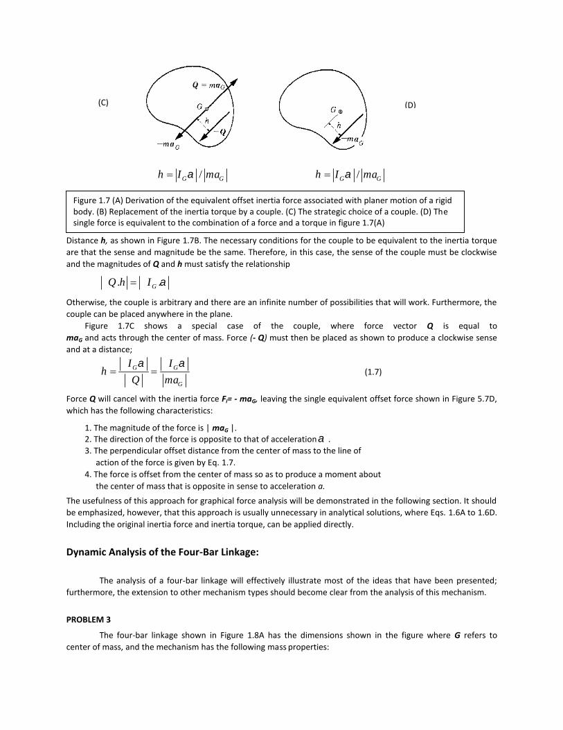
PROBLEM 3

The four-bar linkage shown in Figure 1.8A has the dimensions shown in the figure where G refers tocenter of mass, and the mechanism has the following mass properties:

(C) (D)

/G Gh I ma /G Gh I ma

Figure 1.7 (A) Derivation of the equivalent offset inertia force associated with planer motion of a rigidbody. (B) Replacement of the inertia torque by a couple. (C) The strategic choice of a couple. (D) Thesingle force is equivalent to the combination of a force and a torque in figure 1.7(A)

21 1

22 2

23 3

0.10 20 .

0.20 400 .

0.30 20 .

G

G

G

m kg I kg mm

m kg I kg mm

m kg I kg mm

Determine the instantaneous value of drive torque T required to produce an assumed motion given by inputangular velocity 95 /rad s counterclockwise and input angular acceleration a1 = 0 for the position shown inthe figure. Neglect gravity and friction effects.

SOLUTIONThis problem falls in the first analysis category that is given the mechanism motion, determine the resulting

bearing forces and the necessary input torque. Therefore, the first step in the solution process is to determine the

inertia forces and inertia torques. Thereafter, the problem can be treated as though it were a static-force analysis

problem.

Kinematics analysis of the mechanism can be accomplished by using any of the methods presented in earlier

chapters. Figure 1.8B shows a graphical analysis employing velocity and acceleration polygons. From the analysis,

the following accelerations are determined:

1 1

2 22 2

2 23 3

0( ) 0( )

235,000 312 / 520 /

235,000 308 / 2740 /

C

C

C

a Stationary Center of mass given

a mm Sec rad s ccw

a mm Sec rad s cw

Where the angles of the acceleration vectors are measured counterclockwise from the

positive x direction shown in Figure 5.8A. From Eqs. 1.4A and 1.4B, the inertia

forces and inertia torques are;

Figure 1.8(A) Thefour-bar linkageof Example 5.3

1

22 2 2

23 3 3

1

2 22 2 2

2 23 3 3

0

47,000 132 . / 47 132

30,000 128 . / 30 132

0

208,000 . / 208 .

274,000 . / 274 .

i

i G

i G

i

i G

i G

F

F m a kg mm s N

F m a kg mm s N

C

C I kg mm s cw N mm cw

C I kg mm s ccw N mm ccw

The inertia forces have lines of action through the respective centers of mass, and the inertia torqueses are purecouples.

GRAPHICAL SOLUTIONIn order to simplify the graphical force analysis, we will account for the inertia torques by introducing

equivalent offset inertia forces. These forces are shown in Figure 2.8C, and their placement is determined

according to the previous section. For link 2, the offset force F2 is equal and parallel to inertia force F12.Therefore,

2 47 132F N

It is offset from the center of mass G2 by a perpendicular amount equal to

2 22

2 2

2084.43

47G

G

Ih mm

m a

And this offset is measured to the left as shown to produce the required clockwise direction for the inertiamoment about point G2. In a similar manner, the equivalent offset inertia force for link 3 is

Velocity polygon

Acceleration polygon2

2

2

23

235,000 312 /

520 /

100,000 308 /

2740 /

G

G

a mm Sec

rad Sec ccw

a mm Sec

rad Sec cw

Figure 1.8(B)the velocity andaccelerationanalysisnecessary fordeterminationof inertia forcesand inertiatorques

3 30 128F N at an offset distance 3 33

3 3

2749.13

30G

G

Ih mm

m a

Where this offset is measured to the right from G3 to produce the necessary counterclockwise inertia moment

about G3. From the values of h2 and h3 and the angular relationships, the force positions r2 and r3 in Figure 5.8C are

computed to

be

22 2

33 3 3

45.10cos(132 17 90 )

38.40cos(90 85 128 )

hr BG mm

hr O G mm

Now, we wish to perform a graphical force analysis for known forces F2 and F3. This has been done in ExampleProblem 1.2, and the reader is referred to that

Analysis. The required input torque was found to be T = 383N.mm cw

ANALYTICAL SOLUTIONHaving determined the equivalent offset inertia forces F2 and F3 the analytical solution could proceed

according to Example Problem 9, 6, which examined the same problem. However, it is not necessary to convert to

the offset force, and here we will carry out the analytical solution in terms of the original inertia forces and inertia

couples.

Figure 1.8D shows the linkage with the inertia torques and the inertia forces in xy coordinate form. Consistent with

Figure 1.15A, we define the following quantities:

Figure 1.8(C)Equivalent offsetinertia forces formembers 2 and 3

1 2 3

1 2 3

1 2 3

2 2

3 3

2 3

1 1 1

30 100 50

135 17 85

0 50 25

47 cos(132 ) 31.40 47sin(132 ) 34.90

30cos(128 ) 18.50 30sin(128 ) 23.60

208 . 274 .

0

x y

x y

x y

mm mm mm

r r mm r mm

F N F N

F N F N

C N mm C N mm

F F C

Where the differences are due to round off:

11 21 1

12 22 2

49.8 29.2 786

4.36 95.6 1920

a a b

a a b

Then, 23 12

03 01

31.30 50.30

49.20 50.30

F N F N

F N F N

And 851 .T N mm

Thus, it can be seen that the general analytical solution of the four-bar linkage

presented in this Chapter for static-force analysis is equally well suited for dynamic-

force analysis. Before leaving this example, a couple of general comments should be made.

First, the torque determined is the instantaneous value required for the prescribed motion, and the value will vary

with position. Furthermore, for the position considered, the torque is opposite in direction to the angular velocity

of the crank. This can be explained by the fact that the inertia of the mechanism in this position is tending to

accelerate the crank in the counterclockwise direction, and, therefore, the required torque must be clockwise to

maintain a constant angular speed. If a constant speed is to be maintained throughout the mechanism cycle, then

there will be other positions of the mechanism for which the required torque will be counterclockwise. The second

comment is that it may be impossible to find a mechanism actuator, such as an electric motor, that will supply the

required torque versus position behavior. This problem can be alleviated, however, in the case of a "constant"

Figure 1.8(D)Combinations of inertiaforces and inertiatorques for members 2and 3

rotational speed mechanism through the use of a device called a flywheel, which is mounted on the input shaft

and produces a relatively large mass moment of inertia for crank 1. The flywheel can absorb mechanism torque

and energy- variations with minima] speed fluctuation and. thus, maintains an essentially constant input speed. In

such a case. The assumed-motion approach to dynamic-force analysis is appropriate.

Dynamic Analysis of the Slider-Crank Mechanism:

Dynamic forces are a very important consideration in the design of slider crank mechanisms for use in

machines such as internal combustion engines and reciprocating compressors. Dynamic-force analysis of this

mechanism can be carried out in exactly the same manner as for the four-bar linkage in the previous section.

Following such a process a kinematics analysis is first performed from which expressions are developed for the

inertia force and inertia torque for each of the moving members, These quantities may then be converted to

equivalent offset inertia forces for graphical analysis or they may be retained in the form of forces and torques for

analytical solution, utilizing, in either case, the methods presented in this chapter. In fact, the analysis of the slider

crank mechanism is somewhat easier than that of the four-bar linkage because there is no rotational motion and,

in turn, no inertia torque for the piston or slider, which has translating motion only. The following paragraphs will

describe an analytical approach in detail.

Figure 1.9A is a schematic diagram of a slider crank mechanism, showing the crank 1, the connecting rod 2,and the piston 3, all of which are assumed to be rigid.The center of mass locations are designated by letter G, andthe members have masses m, and moments of inertia IGi, i = 1, 2, 3. The following analysis will consider therelationships of the inertia forces and torques to the bearing reactions and the drive torque on the crank, at anarbitrary mechanism position given by crank angle Friction will be neglected.

Figure 1.9B shows free-body diagrams of the three moving members of the linkage. Applying the dynamicequilibrium conditions. Eqs. 1.6A to 1.6D, to eachmember yields the following set of equations. For the piston (moment equation notincluded):

23 3 3( ) 0x GF m a (1.8A)

03 23 0y yF F (1.8B)

Figure 1.9(A) Dynamic-force analysis of aslider crankmechanism

For the connecting rod (moments about point B):

12 32 2 2( ) 0x x G xF F m a (1.8C)

12 32 2 2( ) 0y y G yF F m a (1.8D)

32 32 2 2

2 2 2 2

sin cos ( ) sin

( ) cos ( ) 0x y G x G

G y G G

F F m a

m a I

(1.8E)

For the crank (moments about point O1):

01 21 1 1( ) 0x x G xF F m a (1.8F)

01 21 1 1( ) 0y y G yF F m a (1.8G)

1 21 21 1 1

1 1 1 1

sin cos ( ) sin

( ) cos ( ) 0x y G x G

G y G G

T F r F r m a r

m a r I

(1.8H)

Where T is the input torque on the crank. This set of equations embodies both of the dynamic-forceanalysis approaches described in Newton's Laws. However, its form isbest suited for the case of known mechanism motion, as illustrated by the followingexample.

Question 1:The four-bar mechanism of Figure has one external force P = 200 Ibf and one inertia force S = 150 Ibf

acting on it. The system is in dynamic equilibrium as a result of torque T2 applied to link 2. Find T2 and the pinforces.(a) Use the graphical method based on free-body diagrams.

Figure 1.9(B) Free-body diagrams of the moving members

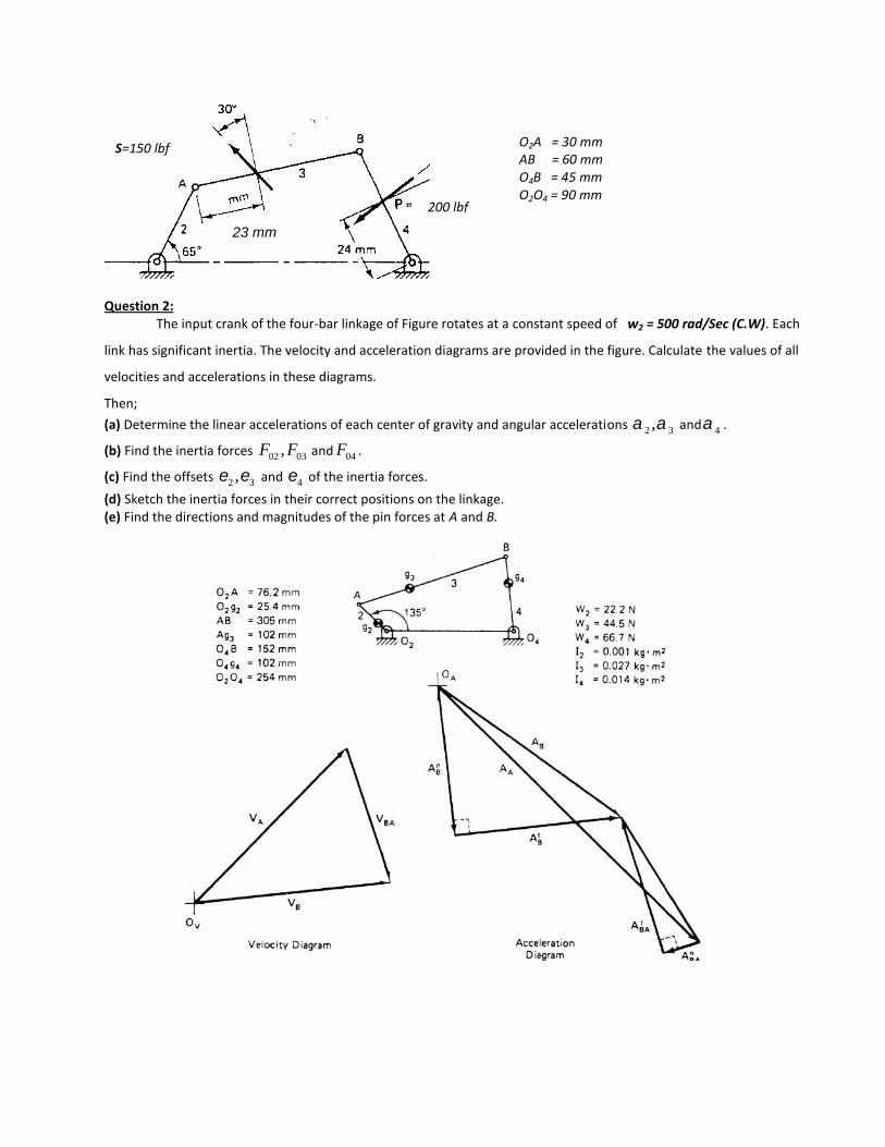
Question 2:The input crank of the four-bar linkage of Figure rotates at a constant speed of w2 = 500 rad/Sec (C.W). Each

link has significant inertia. The velocity and acceleration diagrams are provided in the figure. Calculate the values of all

velocities and accelerations in these diagrams.

Then;(a) Determine the linear accelerations of each center of gravity and angular accelerations 2 3, and 4 .

(b) Find the inertia forces 02 03,F F and 04F .

(c) Find the offsets 2 3, and 4 of the inertia forces.(d) Sketch the inertia forces in their correct positions on the linkage.(e) Find the directions and magnitudes of the pin forces at A and B.

O2A = 30 mmAB = 60 mmO4B = 45 mmO2O4 = 90 mm

200 lbf

23 mm

S=150 lbf

Question 3:The slider-crank mechanism of Figure is to be analyzed to determine the effect of the inertia of the

connecting rod (link 3). The velocity diagram is shown in the figure and the magnitude of VA is given. Calculate the

crank vector O2A and the input angular velocity W2, and proceed to calculate the values of all vectors in the velocity

diagram. Then;

(a) Determine the linear acceleration of the center of gravity of link 3 and the angular acceleration 3 .(b) Find the inertia force F03 of the coupler link.(c) Find the offset 3 of the inertia force F03.(d) Sketch the inertia force in its correct position on the linkage.(e) Find the directions and magnitudes of the pin forces at A and B.(f) Determine the required input torque to drive this mechanism in this position under the conditions described in

this problem.

Question 4:

(a) Find the magnitude Ag4.(b) Find the angular accelerator 4 .(c) What is the magnitude of the inertia force F04?(d) What is the magnitude of the offset 4 ?(e) Draw the vector F04 in the correct location on the mechanism.(f) Given that the mechanism is driven by an input torque, TIN, applied to link 2. Determine the following:

magnitudes of all pin forces, and magnitude and direction of the input torque.

AB = 4 inAG3 = 3 inO2B = 5.5 inM3 = 3 slugsI3 = 12 slug.in2

VA = 20 in/Sec

Flywheel

Application of slider-crank mechanism can be found in reciprocating (steam) engines in the power plant i.e.

internal combustion engines, generators to centrifugal pumps, etc. Output is non-uniform torque from crankshaft;

accordingly there will be fluctuation is speed and subsequently in voltage generated in the generator that is

objectionable or undesirable. Output torque at shaft is required to be uniform. Other kind of applications can be in

punch press. It requires huge amount of power for small time interval. Remaining time of cycle it is ideal. Large

motor that can supply huge quantity of energy for a small interval is required. Output power at piston is required to

be non-uniform. These can be overcome by using flywheel at the crank- shaft. This will behave like a reservoir of

O2B = 80 mmBC = 160 mmO4C = 100 mmO4G4 = 50 mmO2G4 = 200 mm

TCA

168,000 mm/Sec2

578,000 mm/Sec2

( )TCBA

255,000 mm/Sec2

b 4000 mm/Sec2

NCRA

288,000 mm/Sec2

AC = AB + ACB

energy. This will smoothen out the non-uniform output torque from crankshaft. Also it will store energy during the

ideal time and redistribute during the deficit period.

Turning moment diagrams and fluctuations of the crank shaft speed:

A turning moment (crank torque) diagram for a four-stroke internal combustion engine is shown in Figure 1. The

complete cycle is of 720º. From the static and inertia force analyses T −θ can be obtained (at interval of 15º or 5º

preferably).

Engine turning moment diagram:

mean torque input to flywheeloutput fromflywheel

Crank L A B C D E FM

torque720

°T

O 180°

360°

540° °

Pcrank angle

Figure 1 Turning moment diagram

Torque is negative in some interval of the crank angle, it means energy is supplied to engine during this period i.e.

during the compression of the gas and to overcome inertia forces of engine members. This is supplied by the

flywheel (and inertia of engine members), which is attached to the crankshaft. When flywheel is attached to the

crankshaft. LM in diagram shown is the mean torque line. It is defined as

N

∑Ti

T = i=1 (1)m N

If, Tm = 0 then no net energy in the system, Tm ⟩0 then there is an excess of the net energy in the system

and Tm ⟨0 then there is a deficit of the net energy in the system. Area OLMP = net (energy) area of

turning moment diagram = Tm (4π ) . During interval AB, CD and EF , the crank torque is more than the

mean torque means hence excess of energy is supplied to crank i.e. it will accelerate (ω ↑) . During other

interval i.e LA, BC, DE and FM, the crank torque T is less than the mean torque Tm i.e. there is deficit in

energy i.e. crank will decelerate (ω ↓) .

F1 ma F2

F -ma-F =0a 1 2

-maFigure 2 Linear acceleration of a body

ITorque T

TL

T due to load

Torque fromT-TLcrank shaft

Tm

d

Figure 3 Angular acceleration of a body Figure 4 T-θ diagram

From Newton’s second law, we have

∑T = Iα

T − TL = Iα (2)

with

α = d ω =d ω d θ = ω dω (3)dθdt d θ dt

Substituting eqn. (3) in (2), we get

T − TL = Iω dω or (T − TL )dθ = Iω dω (4)dθ

Integrating θ from θω =ωmin

to θω−ωmax

and ω from ωmin to ωmax , we getθ

ωmaxω

max(ω max

2 − ωmin2 )E = ∫ (T − TL )dθ = ∫ Iωdω = 1 I (5)2

θωmin

ωmin

where E is the net area in T-θ diagram between θω and θω , and I is the polar mass moment ofmin max

inertia. A plot of shaft torque versus crank angle θ shows a large variation in magnitude and sense of torque as

shown in Figure 4. Since in same phases the torque is in the same sense as the crank motion and in other phases the

torque is opposite to the crank motion. It would seem that the assumption of constant crank speed is invalid since a

variation in torque would produce a variation in crank speed in the cycle. However, it is usual and necessary to fix a

flywheel to the crankshaft and a flywheel of relatively small moment of inertia will reduce crank speed variations to

negligibly small values (1 or 2% of the crank speed). We cannot change out put torque from the engine (it is fixed)

but by putting flywheel we can regulate speed variation of crankshaft in cycle.

Our interest is to find maximum and minimum speeds and its positions in Figure 5. Points A, B, C, D, E and F are

the points where T −θ diagram cuts the mean torque line. These points are transition points from deficit to extra

energy or vice versa. So crank starts accelerate from deceleration from such points or vice versa. For example at

points: A, C, E → accelerate and at B, D, F → decelerate. At all such points have zero velocity slope i.e. having

velocity maximum or minimum. Crank speed diagram can be drawn qualitatively (approximately) as shown in

Figure 5, where c is the minimum speed location. Area of turning moment diagram represents energy for a particular

period. Net energy between the maximum speed and the minimum speed instant is termed as fluctuation of energy.

For this case area of diagram between C and D or between D and C through points E, F, M, L, A, B and C. Turning

moment diagram for multi cylinder engine can be obtained by T −θ of individual engine by super imposing them in

proper

phase. For a four cylinder (four-stroke) engine the phase difference would be 720º/4=180º or for a six cylinder four-

stroke engine the phase difference = 720º/6= 120º.

Torque due to ram Torque of the flyTL

(Torque from the wheel from theengineflywheel to theCrank T

torque load)T mean T +

torque L MB C D E + FL A +

-- - - P

180 360 540720

crankangle

d maxi. speed

Crank meanf

speed speed e

l a b m

CO

without theflywheel

minimum speed

Figure 5 Fluctuation of the energy

For multi cylinder engine T −θ will be flat compare with single cylinder engine also the difference of maximum and

minimum speed will be less. The coefficient of fluctuation of speed is defined as

δ =ω

max−ω

min (6)ωS

with

ω =ω

max+ω

min (7)2

where ω is the average speed. The fluctuation of energy, E, is represented by corresponding area in

T −θ diagram as

E = 2 I ( ω max − ω min ) = I (ω max + ωmin ) ( ω max − ω min ) = δ S Iω2

(8)1 2 2

2

55

By making I as large as possible, the fluctuation of speed can be reduced for the same fluctuation of energy.

For the disc type flywheel the diameter is constrained by the space and thinness of disc by stress

I = 1 Mr2 with k = r / 2 (9)2

where r is the radius of the disc and k is the radius of gyration. For rim type flywheel diameter is restricted by

centrifugal stresses at rim

I = Mr2 with k = r (10)m m

Equation (9) or (10) gives the mass of rim. The mass of the hub and the arm also contribute by small amount to I,

which in turn gives the fluctuation of speed slightly less than required. By experience equation (10) gives total mass

of the flywheel with 90% of the rim & 10% for the hub and the arm. Typical values of the coefficient of fluctuation

are δ S = 0.002 to 0.006 for electric generators and 0.2 for centrifugal pumps for industrial applications.

Flywheel:

A rigid body rotating about a fixed point with an angular velocity ω (rad/s) and having mass moment of inertia I

(kg-m2) about the same point, the kinetic energy will be

T = 1 Iω2 (11)2

For a flywheel having the maximum speed is ωmax and the minimum speed is ωmin the change in the

kinetic enegy or fluctuation of energy E = I (ω max2 − ωmin

2 )/2 . Let V is the linear velocity of a point at a

radius r from the center of rotation of flywheel E can be written as

E = 0.5Ir2 (Vmax2 −Vmin

2 ) (12)

Also coefficient of fluctuation can be written as

δ =ω

max−ω

min=

Vmax

−Vmin

S ω V

with

V=V

max+V

min

2

Rimr

hub

Arm

Figure 6 A rim type flywheel

(13)

(14)

r k =r

2

Disc-typer flywheel

(automobile)

Rim-type flywheel(i) For rim k=r(for steam engine

or punch press)

Figure 7 Polar mass moment of inertia of rim and disctype flywheel

Combining equations (13) and (14) with equation (12), we get

E = Iδ 2ω2 =I δ V 2

with I = mk2S

r2

Equation (15) becomes

E = mδ S k 2ω2 = mδS k 2V 2

r2

Mass of flywheel (or polar mass moment of inertia) can be obtained as

E Er2M= = E Er 2

I = =δ k 2 ω 2 δ k 2V 2δ S ω 2 δ S ω 2

S S

(15)

(16)

(17)

On neglecting the effect of arm and hub, k can be taken as the mean radius of rim rm . Taking r = rm , and

k = rm , we get

M = E (18)δ V 2S

On using equation (13), we get

M =

2E

(19)(Vmax2 −Vmin

2 )

Since Vmax2 −Vmin

2=(Vmax +Vmin

)2(Vmax −Vmin ) =V (2δSV ) , hence

2

δSV 2 = 0.5(Vmax2 −Vmin

2 ) (20)

Equations (18) or (19) can be used for finding mass of the flywheel. The 90% of M will be distributed at rim and

10% for the hub and arms. By experience the maximum velocity Vmax is limited by the material and centrifugal

stresses at the rim.

Flywheel of a Punch Press:

Let d be the diameter of hole to be punched, t is the thickness of plate to be punched, fsmax is the

resistance to shear (shear stress), T is the time between successive punch (punching period), tp is the

time for the actual punching operation. (≈ 0.1T ) and N is speed of motor in rpm to which the flywheel is attached.

Experiments show that: (i) the maximum force P occurs at time = (3/8)tp and (ii) the area under the actual force

curve i.e. the energy required to punch a hole is equal to rectangular area (shaded area), hence

Energy required for punching a hole W = Pt /2 (21)

In other words the average force is half the maximum force.

max. forceActual force variation

forceaverage force d

t

P/2

tdispalcement

Figure 8 Punching force variation with deformations

Maximum force required to punch a hole

P=fs max

πdt

Combining equations (21) and (22), it gives

W=

0.5Pt=

0.5( fsmax π

dt )t

where fsmax is in N/m2, d in m, t in m, W in N-m and tp in sec. Average power during punching

0.5( fs max π d t2 )

W/(time for actual punching) = Watttp

(22)

(23)

(24)

Hence, in absence of the flywheel the motor should be capable of supplying large power instantly as punching is

done almost instantaneously. If flywheel is attached to the motor shaft, then the flywheel store energy during ideal

time and will give back during the actual punching operation

Average power required from motor = W/(Punching interval) =0.5( f

s max π d t2 )Watt (25)

T

Average power from eqn. (25) will be for less than that from equation (24) (e.g. of the order of 1/10).

Steam engine Punch PressI

T( ) TL T TL( )T( ) - TL= I I

Figure 9 (a) Steam engine Figure 10(a) Punch press

T( )

min +_ maxTm=T

L

O

4T N

Figure 9(b) A turning moment diagram

kTotal energy

consumed

max minP

TV J L

M4 0

Figure 10(b) A turning moment diagram

In Figure 10(b) the total energy consumed during ωmax and ωmin = area IJLM.

The total energy supplied in period during same period (ωmax to ωmin ) =area IVPM

Hence, the fluctuation of the energy E= IJLM-IVPM = area NOPM – area IVPM.

kEnergy requiredfor punching

Power constantEnergy supplied max minby motor

O V J L PN

I MTimetP

One full cycle T

Figure Turning moment diagram if a punch press

Hence,

1/ 2 fSπ dt 2 1/ 2 fSπ dt 2

E = ×T − tp

T T

The fluctuation of energy will be the power supplied by the motor during the ideal period. Whatever energy is

supplied during the actual punching will also be consumed in the punching operation. Maximum speed will occurs

just before the punching and minimum speed will occur just after the punching. The net energy gained by the

flywheel during this period i.e. from the minimum speed to the maximum speed (or vice versa) will be the

fluctuation of energy. The mass of flywheel can be obtained by:

M = E /δ V 2for given δ S and V , once E is calculated from eqn. (26).

S

Location of the maximum and minimum speeds:

Let Ai be the area of the respective loop, ωo is the speed at start of cycle (datum value). We will take datum at

starting point and will calculate energy after every loop. At end of cycle total energy should be zero. The maximum

speed is at the maximum energy (7 units) and the minimum speed is at the minimum

energy (-2 units). E = Net area between ωmax and ωmin (-4+2-7=-9 units) or between

(4-3+2-1+7=9 units) = 0.5I (ω max2

− ωmin2 ) .

Location of maximum and minimum speeds:Energy

after0 7 3 5 -2 2 -1 1

0T A =7 A =4each 1

A2=25

A7=2loop +

min+

0 max + +T

av

(datum) - - - -

O A =4 A =7 A =3 A9=14 6

2 Engine cycle

Figure 12 Turning moment diagram

Analytical expressions for turning moment: The crankshaft torque is periodic or repetitive in

nature (over a cycle), so we can express torque as a sum of harmonics by Fourier analysis

T=T(θ) = C + A sinθ + A sin2θ + ⋅⋅⋅⋅ + A sinnθ + ⋅⋅⋅⋅ + B cosθ + B cos2θ + ⋅⋅⋅⋅ + B cosnθ + ⋅⋅⋅ (27)0 1 2 n 1 2 n

With the knowledge of T(θ), C0 , A1 , A2 ⋅⋅⋅⋅ can be obtained. For all practical purpose first few harmonics will

give a sufficient result. This will be very useful in analysis of torsional vibration of engine rankshaft. We will use

this analysis for finding mass of flywheel. Let period of T(θ) is 360°, then

2π

Work done per revolution = ∫ T (θ )dθ = C0 2π (28)0

and1 2π 1

Mean torque = Tm = ∫ T (θ )dθ = C0 2π = C0 (29)2π 2π0

Now we have to obtain the intersection point of “T(θ)- θ “ curve with Tm line. Putting T − Tm = 0 in (27),

we can get θ , as

ωmin

and ωmax

T(θ ) − T = 0 = A sinθ + A sin2θ + ⋅⋅⋅ + A sinnθ + ⋅⋅⋅ + B cosθ + B cos2θ + ⋅⋅⋅ + B cosnθ + ⋅⋅⋅m 1 2 n 1 2 n

which gives

A sinθ + A sin2θ + ⋅⋅⋅ + A sinnθ + ⋅⋅⋅ + B cosθ + B cos2θ + ⋅⋅⋅ + B cosnθ + ⋅⋅⋅ = 0 (30)1 2 n 1 2 n

Equation (30) is a transdental (non-linear) eqn. in terms of θ , from which we can get θ = θ1 ,θ2

⋅⋅⋅⋅ . Let during period of 360° two intersections θ1 and θ2 are there, then the fluctuation of

energy can be obtained as (Figure 13):

θ2(31)E = ∫ (T(θ )− Tm )dθ

θ1

T( )one cycle

min + max

- Tm-

2

Fly wheel for reciprocating machinery installationFigure 13

Example 1: A single-cylinder, four- stroke oil engine develops 25 kW at 300 rpm. The work done by

the gases during expansion stroke is 2.3 times the work done on the gases during compression

stroke and the work done during the suction and exhaust strokes is negligible. If the turning moment

diagram during expansion is assumed to be triangular in shape and the speed is to be maintained

within 1% of the mean speed, find the moment of inertia of the flywheel.

Solution: Given data are: δ s = 0.02 ; P = 25 kW; Wexp = 2.3Wcomp ;

ω = 3000 rpm = 2π 300/60 = 100π rad/s = 31.41 rad/s ;

Tav = P /ω = 25× 103 /(100π ) = 2500/π Nm = 795.8 Nm (In Figure 14 height: AC)

Total work done in one cycle (i.e. 4π rad. rotation) Wtotal = Tav 4π = (2500/π ) 4π =10000 Nm

We have,

Wtotal

= Wexp

−Wcomp hence 10000 = 2.3Wcomp −Wcomp

which gives

Wcomp = 7692.3 Nm and Wexp =17692.3 Nm

Tmax.B

TE

a bT

av.c D

O A 2 3 4

Figure 14 Turning moment diagram

Work done during expansion stroke: (1/2)Tmaxπ = Wexp =17692.3, which gives Tmax =11263.3 N.m = AB .

BC = maxi. excess turning moment = Tmax − Tav = AB - AC =11263.3 − 795.8 =10467.5 Nm .

Hence the fluctuation of energy is E =( )

BC×ab1/2

ODB & abB are similar, hence ab/π = BC/AB or ab = π (10467.5/11263.3) or ab = 2.92 .

Which gives E = (1/2)10467.5× 2.92 =15280.6 Nm

We have E = I δsWav 2 or I =15280.6/{0.02× ( 31.40.6)2} = 774.4 kg-m2

Or

E = W 1−(AC / AB 2 =17.692 1− (0.795733/11.7631) 2 =15.28 Nm

exp ) [ ]OrFrom similar OBD & aBD : ab / OD = BC / AB

E

Area Bab (1/2) ab × BC ab BC BC BC BC 2 10467.5 2

= = = = =Area OBD (1/2)OD × AB 11263.3OD AB AB AB AB

Wexp

Area Bab = E = (10467.5/11263.3)2 × 17692.3 =15280.55 Nm

Example 2. The vertical scale of the turning moment diagram for a multi-cylinder engine, shown in

Figure 15, is 1 cm = 7000 Nm of torque, and horizontal scale is 1 cm = 300 of crank rotation. The

areas (in cm2) of the turning moment diagram above and below the mean resistance line, starting

from A in Figure @ and taken in order, are 0.5, +1.2, -0.95, +1.45, -0.85, +0.71, -1.06. The enginespeed is 800 rpm and it is desired that the fluctuation from minimum to maximum speed should notbe more then 2% of average speed. Determine the moment of inertia of the flywheel.

M (Torque)

M A B C D E F G H (≡ A)

N.m

θFigure 15 Example 2

Solution:

mini maxi0 -0.5 0.7 -0.25 1.2 0.35 1.06 0

M A B C D E F G HN.M

ωmin ωmax

θFigure 16 Fluctuation of the energy

E = E − E = 1.2 − (−0.5) = 1.7 cm2 ≡ 1.7× 7000× π 30 = 6230.825N-mmax min 180

ω = 800 rpm = 83.776 rad/s and δs = 0.02

Hence,

I = E = 44.39 kgm2

ω 2 δ s

Exercise Problems:

(1) The following data refers to a single-cylinder four cycle diesel engin: speed = 2500 rpm, stroke = 25 cm,

diameter of cylinder = 21 cm, length of connecting rod = 44 cm, CG of connecting rod is 18 cm from crank pin

center, time for 60 complete swings of the connecting rod about piston pin = 72 s, mass of connecting rod = 4.5 kg,

mass of piston with rings = 2.5 kg, equivalent mass of crank at crank radius = 2 kg, counterbalance mass of the crank

at crank radius = 2 kg, piston pin, crank pin and main bearing diameters 2, 8 and 8 cm respectively. The indicator

card is assumed as an idealised diesel cycle,which can be described as follows: The compression starts with an initial

pressure of 0.1 MPa and the law of compression curve is given by the exponent 1.4. The compression ratio is 16.

The fuel is admitted for 30% of the stroke, at constant pressure and the expansion law is given by the exponent 1.4,

which takes place at the end of the stroke. The exhaust and suction takes place at constant pressure of 0.1 MPa.

Suggest a suitable flywheel for this engine if the coefficient of fluctuation of speed is 0.03.

(2) Twenty 1-cm holes are to be punched every minute in a 1.5 cm plate whose resistance to shear is 35316

N/cm2. The actual punching takes place in one-fifth of the interval between successive operations. The speed of the

flywheel is 300 rpm. Making the usual assumptions specify the dimensions of a suitable CI rimmed flywheel. Use

coefficient of fluctuation of speed = 0.01 and V = 60 m/s.

(3) The equation of a turning moment curve of an IC engine running at 300 rpm is given by

T = [25000 + 8500 sin3θ ]. A flywheel coupled to the crankshaft has a moment of inertia 450 kg m2 about the axis

of rotation. Determine (a) Horse power of the engine (b) total percentage fluctuation of speed (c) maximum angle by

which the flywheel leads or lags an imaginary flywheel running at a constant speed of 300 rpm.

(4) The turning moment diagram for a multi cylinder IC engine is drawn to the following scales

1 cm = 15o crank angle

1 cm = 3 k Nm

During one revolution of the crank the areas with reference to the mean torque line are 3.52, () 3.77,

3.62, () 4.35, 4.40 and (–) 3.42 cm2. Determine mass moment of inertia to keep the fluctuation of mean

speed within 2.5% with reference to mean speed. Engine speed is 200 rpm.

(5)A single cylinder four-stroke petrol engine develops 18.4 kW power at a mean speed of 300 rpm. The

work done during suction and exhaust strokes can be neglected. The work done by the gases during

explosion strokes is three times the work done on the gases during the compression strokes and they can

be represented by the triangles. Determine the mass of the flywheel to prevent a fluctuation of speed

greater than 2 per cent from the mean speed. The flywheel diameter may be taken as 1.5 m.

(6) A three cylinder two-stroke engine has its cranks 120o apart. The speed of the engine is 600 rpm. The

turning moment diagram for each cylinder can be represented by a triangle for one expansion stroke with

a maximum value of one stroke with a maximum value of 600 Nm at 60o from the top dead centre. The

turning moment in other stroke is zero for all the cylinders. Determine :

(a) the power developed by the engine,

(b) the coefficient of fluctuation of speed with a flywheel having mass 10 kg and radiusof gyration equal to 0.5 m,

(c) the coefficient of fluctuation of energy, and

(d) the maximum angular acceleration of the flywheel.