Unifying evolutionary dynamics: From indivi dual ...math.arizona.edu/~jwatkins/06TPBchampagnat.pdf · Unifying evolutionary dynamics: From indivi dual stochastic processes to macroscopic

Theoretical Population Biology 69 (2006) 297–321

Unifying evolutionary dynamics: From individual stochastic processesto macroscopic models

Nicolas Champagnata,b, Regis Ferrierea,c,!, Sylvie Meleardb

aLaboratoire d’Ecologie, Equipe Eco-Evolution Mathematique, Ecole Normale Superieure, 46 rue d’Ulm, 75230 Paris Cedex 05, FrancebEquipe MODAL’X Universite Paris 10, 200 avenue de la Republique, 92001 Nanterre Cedex, FrancecDepartment of Ecology and Evolutionary Biology, University of Arizona, Tucson, AZ 85721, USA

Received 14 June 2005Available online 7 February 2006

Abstract

A distinctive signature of living systems is Darwinian evolution, that is, a propensity to generate as well as self-select individualdiversity. To capture this essential feature of life while describing the dynamics of populations, mathematical models must be rooted inthe microscopic, stochastic description of discrete individuals characterized by one or several adaptive traits and interacting with eachother. The simplest models assume asexual reproduction and haploid genetics: an offspring usually inherits the trait values of herprogenitor, except when a mutation causes the offspring to take a mutation step to new trait values; selection follows from ecologicalinteractions among individuals. Here we present a rigorous construction of the microscopic population process that captures theprobabilistic dynamics over continuous time of birth, mutation, and death, as influenced by the trait values of each individual, andinteractions between individuals. A by-product of this formal construction is a general algorithm for efficient numerical simulation of theindividual-level model. Once the microscopic process is in place, we derive different macroscopic models of adaptive evolution. Thesemodels differ in the renormalization they assume, i.e. in the limits taken, in specific orders, on population size, mutation rate, mutationstep, while rescaling time accordingly. The macroscopic models also differ in their mathematical nature: deterministic, in the form ofordinary, integro-, or partial differential equations, or probabilistic, like stochastic partial differential equations or superprocesses. Thesemodels include extensions of Kimura’s equation (and of its approximation for small mutation effects) to frequency- and density-dependent selection. A novel class of macroscopic models obtains when assuming that individual birth and death occur on a shorttimescale compared with the timescale of typical population growth. On a timescale of very rare mutations, we establish rigorously themodels of ‘‘trait substitution sequences’’ and their approximation known as the ‘‘canonical equation of adaptive dynamics’’. We extendthese models to account for mutation bias and random drift between multiple evolutionary attractors. The renormalization approachused in this study also opens promising avenues to study and predict patterns of life-history allometries, thereby bridging individualphysiology, genetic variation, and ecological interactions in a common evolutionary framework.r 2006 Elsevier Inc. All rights reserved.

Keywords: Adaptive evolution; Individual-based model; Birth and death point process; Body size scaling; Timescale separation; Mutagenesis; Density-dependent selection; Frequency-dependent selection; Invasion fitness; Adaptive dynamics; Canonical equation; Nonlinear stochastic partial differentialequations; Nonlinear PDEs; Large deviation principle

1. Introduction

Evolutionary biology has long received the enlight-enment of mathematics. At the dawn of the twentiethcentury, Darwinian evolution was viewed essentially as aformal theory that could only be tested using mathematical

and statistical techniques. The founding fathers of evolu-tionary genetics (Fisher, Haldane and Wright) usedmathematical models to generate a synthesis betweenMendelian genetics and Darwinian evolution that pavedthe way toward contemporary models of adaptive evolu-tion. However, the development of a general and coherentframework for adaptive evolution modelling, built from thebasic stochastic processes acting at the individual level, isfar from complete (Page and Nowak, 2002). Mathematical

ARTICLE IN PRESS

www.elsevier.com/locate/tpb

0040-5809/$ - see front matter r 2006 Elsevier Inc. All rights reserved.doi:10.1016/j.tpb.2005.10.004

!Corresponding author. Fax: +331 4432 3885.E-mail address: [email protected] (R. Ferriere).

http://www.elsevier.com/locate/tpb

models of adaptive evolution are essentially phenomen-ological, rather than derived from the ‘first principles’ ofindividual birth, mutation, interaction and death. Here wereport the rigorous mathematical derivation of macro-scopic models of evolutionary dynamics scaling up fromthe microscopic description of demographic and ecologicalstochastic processes acting at the individual level. Ouranalysis emphasizes that different models obtain dependingon how individual processes are renormalized, andprovides a unified framework for understanding how thesedifferent models relate to each other.

Early models of adaptive evolution pictured the muta-tion-selection process as a steady ascent on a so-called‘adaptive landscape’, thereby suggesting some solid groundover which the population would move, under the pressureof environmental factors (Wright, 1969). The next theore-tical step was to recognize that the adaptive landscapemetaphor misses one-half of the evolutionary process:although the environment selects the adaptations, theseadaptations can shape the environment (Haldane, 1932;Pimentel, 1968; Stenseth, 1986; Metz et al., 1992). There-fore, there is no such thing as a pre-defined adaptivelandscape; in fact, the fitness of a phenotype depends uponthe phenotypic composition of the population, andselection generally is frequency-dependent (Metz et al.,1992; Heino et al., 1998). Throughout the last 50 years thisviewpoint spread and affected not only the intuition ofevolutionary biologists, but also their mathematical tools(Nowak and Sigmund, 2004). The notion of adaptivelandscape across mathematical evolutionary theories isreviewed in Kirkpatrick and Rousset (2004).

Game theory was imported from economics intoevolutionary theory, in which it became a popular frame-work for the construction of frequency-dependent modelsof natural selection (Hamilton, 1967; Maynard Smith andPrice, 1973; Maynard Smith, 1982; Hofbauer and Sig-mund, 1998, 2003; Nowak and Sigmund, 2004). Withadaptive dynamics modelling, evolutionary game theorywas extended to handle the complexity of ecologicalsystems from which selective pressures emanate. However,the rare mutation and large population scenario assumedby adaptive dynamics modelling implies that the complex-ity of stochastic individual life-history events is sub-sumed into deterministic steps of mutant invasion-fixation,taking place in vanishingly small time by the wholepopulation as a single, monomorphic entity (Metz et al.,1996; Dieckmann and Law, 1996). Thus, adaptivedynamics models make approximations that bypass ratherthan encompass the individual level (Nowak and Sigmund,2004).

An alternate pathway has been followed by populationand quantitative genetics, domains in which the emphasiswas early on set on understanding the forces that maintaingenetic variation (Burger, 2000). The ‘continuum-of-alleles’model introduced by Crow and Kimura (1964) does notimpose a rare mutation scenario, but otherwise shares thesame basic assumptions as in evolutionary game theory

and adaptive dynamics models: the genetic system involvesone-locus haploid asexual individuals, and the effect ofmutant alleles are randomly chosen from a continuousdistribution. The mathematical study of the continuum-of-alleles model has begun only relatively recently (see Burger,1998, 2000 and Waxman, 2003 for reviews) in a frequency-independent selection framework. The mutation-selectiondynamics of quantitative traits under frequency-dependentselection has been investigated thoroughly by Burger(2005) and Burger and Gimelfarb (2004) in the wake ofBulmer’s (1974), Slatkin’s (1979), Nagylaki’s (1979),Christiansen and Loeschcke (1980) and Asmussen’s(1983) seminal studies. After Matessi and Di Pasquale(1996), among others, had emphasized multilocus geneticsas causing long-term evolution to depart from theWrightian model, Burger’s (2005) approach has taken amajor step forward in further tying up details of the geneticsystem with population demography.Recent advances in probability theory (first applied in

the population biological context by Fournier and Me-leard, 2004 and Champagnat, 2004b) make the time ripefor attempting systematic derivation of macroscopicmodels of evolutionary dynamics from individual-basedprocesses. By scaling up from the level of individuals andstochastic processes acting upon them to the macroscopicdynamics of population evolution, we aim at setting up themathematical framework needed for bridging behavioral,ecological and evolutionary processes (Jansen and Mulder,1999; Abrams, 2001; Ferriere et al., 2004; Dieckmann andFerriere, 2004; Hairston et al., 2005). Our baseline model isa stochastic process describing a finite population ofdiscrete interacting individuals characterized by one orseveral adaptive phenotypic traits. We focus on thesimplest case of asexual reproduction and haploid genetics.The infinitesimal generator of this process captures theprobabilistic dynamics, over continuous time, of birth,mutation and death, as influenced by the trait values ofeach individual and ecological interactions among indivi-duals. The rigorous algorithmic construction of thepopulation process is given in Section 2. This algorithmis implemented numerically and simulations are presented;they unveil qualitatively different evolutionary behaviorsas a consequence of varying the order of magnitude ofpopulation size, mutation probability and mutation stepsize. These phenomena are investigated in the next sections,by systematically deriving macroscopic models from theindividual-based process. Our first approach (Section 3)aims at deriving deterministic equations to describe themoments of trajectories of the point process, i.e. thestatistics of a large number of independent realizations ofthe process. The model takes the form of a hierarchicalsystem of moment equations embedded into each other; thecompetition kernels that capture individual interactionsmake it impossible, even in the simple mean-field case ofrandom and uniform interactions among phenotypes, tofind simple moment closures that would decorrelate thesystem.

ARTICLE IN PRESSN. Champagnat et al. / Theoretical Population Biology 69 (2006) 297–321298

The alternate approach involves renormalizing theindividual-level process by means of a large populationlimit. Applied by itself, the limit yields a deterministic,nonlinear integro-differential equation (Section 4.1). Fordifferent scalings of birth, death and mutation rates, weobtain qualitatively different PDE limits, in which someform of demographic randomness may or may not beretained as a stochastic term (Section 4). More specifically,when combined with the acceleration of birth (hence theacceleration of mutation) and death and an asymptotic ofsmall mutation steps, the large population limit yieldseither a deterministic nonlinear reaction–diffusion model,or a stochastic measure-valued process, depending on theacceleration rate of the birth-and-death process (Section4.2.1). When this acceleration of birth and death iscombined with a rare mutation limit, the large populationapproximation yields a nonlinear integro-differential equa-tion, either deterministic or stochastic, depending againupon the acceleration rate of the birth-and-death process(Section 4.2.2). In Section 5, we assume that the ancestralpopulation is monomorphic and that the timescale ofecological interactions and evolutionary change are sepa-rated: the birth-and-death process is fast while mutationsare rare. In a large population limit, the process convergeson the mutation timescale to a jump process over the traitspace, which corresponds to the trait substitution sequenceof adaptive dynamics modelling (Section 5.1). By rescalingthe mutation step (making it infinitesimal) we finallyrecover a deterministic process driven by the so-called‘‘canonical equation of adaptive dynamics’’ first introducedby Dieckmann and Law (1996) (Section 5.2).

Throughout the paper E!"# denotes mathematical ex-pectation of random variables.

2. Population point process

Our model’s construction starts with the microscopicdescription of a population in which the adaptive traits ofindividuals influence their birth rate, the mutation process,their death rate, and how they interact with each other andtheir external environment. Thus, mathematically, thepopulation can be viewed as a stochastic interactingindividual system (cf. Durrett and Levin, 1994). Thephenotype of each individual is described by a vector oftrait values. The trait space X is assumed to be a subset ofl-dimensional real vectors and thus describes l real-valuedtraits. In the trait space X, the population is entirelycharacterized by a counting measure, that is, a mathema-tical counting device which keeps track of the number ofindividuals expressing different phenotypes. The popula-tion evolves according to a Markov process on the set ofsuch counting measures on X; the Markov propertyassumes that the dynamics of the population after time tdepends on the past information only through the currentstate of the population (i.e. at time t). The infinitesimalgenerator describes the mean behavior of this Markovprocess; it captures the birth and death events that each

individual experiences while interacting with other indivi-duals.

2.1. Process construction

We consider a population in which individuals can givebirth and die at rates that are influenced by the individualtraits and by interactions with individuals carrying the sameor different traits. These events occur randomly, in contin-uous time. Reproduction is almost faithful: there is someprobability that a mutation causes an offspring’s phenotypeto differ from her progenitor’s. Interactions translate into adependency of the birth and death rates of any focalindividual upon the number of interacting individuals.The population is characterized at any time t by the finite

counting measure

nt $XI!t#

i$1

dxit , (2.1)

where dx is the Dirac measure at x. The measure ntdescribes the distribution of individuals over the trait spaceat time t, where I!t# is the total number of individuals aliveat time t, and x1t ; . . . ;x

I!t#t denote the individuals’ traits. The

time process nt evolves in the set of all finite countingmeasures. Note that the total mass of the measure nt isequal to I!t#. Likewise, nt!G# represents the number ofindividuals with traits contained in any subset G of the traitspace, and

Z

Xj!x#nt!dx# $

XI!t#

i$1

j!xit#,

which means that the total ‘‘mass’’ of individuals, each ofthem being ‘‘weighted’’ by the ‘‘scale’’ j, is computed byintegrating j with respect to nt over the trait space.The population dynamics are driven by a birth-muta-

tion-death process defined as follows. Individual mortalityand reproduction are influenced by interactions betweenindividuals. For a population whose state is described bythe counting measure n $

PIi$1dxi , let us define d!x;U %

n!x## as the death rate of individuals with trait x, b!x;V %n!x## as the birth rate of individuals with trait x, where Uand V are the interaction kernels affecting mortality andreproduction, respectively. Here % denotes the convolutionoperator, which means that U and V give the ‘‘weight’’ ofeach individual when interacting with a focal individual, asa function of how phenotypically different they are. Forexample, U % n!x# $

PIi$1U!x& xi#. Mutation-related

parameters are expressed as functions of the individualtrait values only (although there would be no formaldifficulty to include a dependency on the population state,in order to obtain adaptive mutagenesis models): m!x# is theprobability that an offspring produced by an individualwith trait x carries a mutated trait, M!x; z# is the mutationstep kernel of the offspring trait x' z produced byindividuals with trait x. Since the mutant trait belongs toX, we assume M!x; z# $ 0 if x' z does not belong to X.

ARTICLE IN PRESSN. Champagnat et al. / Theoretical Population Biology 69 (2006) 297–321 299

Thus, the individual processes driving the populationadaptive evolution develop through time as follows:

( At t $ 0 the population is characterized by a (possiblyrandom) counting measure n0. This measure gives theancestral state of the population. Whether the ancestralstate is monomorphic or polymorphic will provemathematically important later on.

( Each individual has two independent random exponen-tially distributed ‘‘clocks’’: a birth clock with parameterb!x;V % nt!x##, and a death clock with parameterd!x;U % nt!x##. Assuming exponential distributions al-lows to reset both clocks to 0 every time one of themrings. At any time t:

( If the death clock of an individual rings, this individualdies and disappears.

( If the birth clock of an individual with trait x rings, thisindividual produces an offspring. With probability1& m!x# the offspring carries the same trait x; withprobability m!x# the trait is mutated.

( If a mutation occurs, the mutated offspring instantlyacquires a new trait x' z, picked randomly according tothe mutation step measure M!x; z#dz.

If n $PI

i$1 dxi represents the population state at a giventime t, the infinitesimal dynamics of the population after tis described by the following operator on the set of realbounded functions f (so-called infinitesimal generator):

Lf!n# $XI

i$1

)1& m!xi#*b!xi;V % n!xi##)f!n' dxi # & f!n#*

'XI

i$1

m!xi#b!xi;V % n!xi##

+Z

Rl)f!n' dxi'z# & f!n#*M!xi; z#dz

'XI

i$1

d!xi;U % n!xi##)f!n& dxi # & f!n#*. !2:2#

The first term of (2.2) captures the effect on the populationof birth without mutation; the second term, that of birthwith mutation; and the last term, that of death. The densitydependence of vital rates makes all terms nonlinear.

At this stage, a first mathematical step has to be taken:the formal construction of the process is required to justifythe existence of a Markov process admitting L asinfinitesimal generator. There is a threefold biologicalpayoff to such a mathematical endeavor: (1) providing arigorous and efficient algorithm for numerical simulations(given hereafter); (2) laying the mathematical basis toderive the moment equations of the process (Section 3);and (3) establishing a general method that will be used toderive macroscopic models (Sections 4 and 5).

We make the biologically natural assumption that allparameters, as functions of traits, remain bounded, exceptfor the death rate. Specifically, we assume that for anypopulation state n $

PIi$1 dxi , the birth rate b!x;V % n!x## is

upper bounded by a constant b, that the interaction kernelsU and V are upper bounded by constants U and V , andthat there exists a constant d such that d!x;U % n!x##p!1' I#d. The latter assumption means that the densitydependence on mortality is ‘‘linear or less than linear’’.Lastly, we assume that there exist a constant C and aprobability density M such that for any trait x,M!x; z#pCM!z#. This is implied in particular if themutation step distribution varies smoothly over a boundedtrait space. These assumptions ensure that there exists aconstant C such that for any population state described bythe counting measure n $

PIi$1 dxi , the total event rate, i.e.

the sum of all event rates, is bounded by CI!I ' 1#. Indeed,without density dependence, the per capita event rateshould be upper bounded by C, making the total event rateupper bounded by CI(since I is the size of the population);the influence of density dependence appears through themultiplicative term I ' 1.Let us now give an algorithmic construction of the

population process !nt#tX0. At any time t, we must describethe size of the population, and the trait vector of allindividuals alive at that time. At time t $ 0, the initialpopulation state n0 contains I!0# individuals. The vector ofrandom variables X0 $ !Xi

0#1pipI!0# denotes the corre-sponding trait values. More generally the vector of traitsof all individuals alive at time t is denoted by Xt. Weintroduce the following sequences of independent randomvariables, which will drive the algorithm. First, the valuesof a sequence of random variables !Wk#k2N% with uniformlaw on )0; 1* will be used to select the type of birth or deathevents. Second, the times at which events may be realizedwill be described using a sequence of random variables!tk#k2N with exponential law with parameter C (henceE!tk# $ 1=C). Third, the mutation steps will be driven by asequence of random variables !Zk#k2N with law M!z#dz.We set T0 $ 0 and construct the process inductively over

successive event steps kX1 as follows. At step k & 1,the number of individuals is Ik&1, and the trait vectorof these individuals is XTk&1

. We define Tk $ Tk&1

'tk=Ik&1!Ik&1 ' 1#. The term tk=Ik&1!Ik&1 ' 1# representsthe minimal amount of time between two events (birth ordeath) in a population of size Ik&1 (this is because the totalevent rate is bounded by CIk&1!Ik&1 ' 1#). At time Tk, onechooses an individual ik $ i uniformly at random amongthe Ik&1 alive in the time interval )Tk&1;Tk#; thisindividual’s trait is Xi

Tk&1. (If Ik&1 $ 0 then nt $ 0 for all

tXTk&1.) Because C!Ik&1 ' 1# gives an upper bound on thetotal event rate for each individual, one can decide of thefate of that individual by making use of the following rules:

( If

0pWkpd!Xi

Tk&1;PIk&1

j$1 U!XiTk&1

& XjTk&1

##C!Ik&1 ' 1#

$ Wi1!XTk&1

#,

then the chosen individual dies, and Ik $ Ik&1 & 1.


( If

Wi1!XTk&1

#oWkpWi2!XTk&1#,

where

Wi2!XTk&1

# $ Wi1!XTk&1

#

')1&m!Xi

Tk&1#*b!Xi

Tk&1;PIk&1

j$1V !Xi

Tk&1&Xj

Tk&1##

C!Ik&1'1# ,

then the chosen individual gives birth to an offspringwith the same trait, and Ik $ Ik&1 ' 1.

( If

Wi2!XTk&1

#oWkpWi3!XTk&1

;Zk#,

where

Wi3!XTk&1

;Zk# $ Wi2!XTk&1

#

'm!Xi

Tk&1#b!Xi

Tk&1;PIk&1

j$1V !Xi

Tk&1&Xj

Tk&1##M!Xi

Tk&1;Zk#

CM!Zk#!Ik&1'1# ,

then the chosen individual gives birth to a mutantoffspring with trait Xi

Tk&1' Zk, and Ik $ Ik&1 ' 1.

( If Wk4Wi3!XTk&1

;Zk#, nothing happens, and Ik $ Ik&1.

Mathematically, it is necessary to justify that theindividual-based process !nt#tX0 is well defined on thewhole time interval )0;1#; otherwise, the sequence Tk

might converge to a finite accumulation point at which thepopulation process would explode in finite time. To thisend, one can use the fact that the birth rate remainsbounded. This allows one to compare the sequence of jumptimes of the process nt with that of a continuous-timeGalton–Watson process. Since the latter converges toinfinity, the same holds for the process nt, which providesthe necessary justification.

The process !nt#tX0 is Markovian with generator Ldefined by (2.2). From this follows the classical probabil-istic decomposition of nt as a solution of an integro-differential equation governed by L and perturbed by amartingale process (Ethier and Kurtz, 1986). In particular,(2.2) entails that for any function j, bounded andmeasurable on X

Z

Xj!x#nt!dx# $ mt!j# '

Z

Xj!x#n0!dx#

'Z t

0

Z

X!!1& m!x##b!x;V % ns!x##

& d!x;U % ns!x###j!x#ns!dx#ds

'Z t

0

Z

Xm!x#b!x;V % ns!x##

+Z

Rlj!x' z#M!x; z#dz

! "ns!dx#ds,

!2:3#

where the time process mt!j# is a martingale (see appendix)which describes the random fluctuations of the Markovprocess n. For each t, the random variable mt!j# has mean

zero and variance equal to:Z t

0

Z

Xj2!x#!!1& m!x##b!x;V % ns!x## ' d!x;U % ns!x###

#

'm!x#b!x;V % ns!x##Z

Rlj2!x' z#M!x; z#dz

$ns!dx#ds.

!2:4#

This decomposition, developed in the appendix, will be thekey to our approximation method. Eq. (2.3) can beunderstood as providing a general model for the ‘pheno-typic mass’ of the population that can be associated withany given ‘scale’ j, j!x# being the ‘weight’ of trait x in thephenotypic space X.

2.2. Examples and simulations

A simple example assumes logistic density dependencemediated by the death rate only:

b!x; z# $ b!x#; d!x; z# $ d!x# ' a!x#z, (2.5)

where b, d and a are bounded functions. Then

d!x;U % n!x## $ d!x# ' a!x#Z

XU!x& y#n!dy#. (2.6)

Note that, in the case where m , 1, the individual-basedmodel can also be interpreted as a model of ‘‘spatiallystructured population’’, where the trait is viewed as aspatial location and mutation is analogous to dispersal.This is the type of models studied by Bolker and Pacala(1997, 1999), Law et al. (2003) and Fournier and Meleard(2004). The well-known case U , 1 corresponds to densitydependence involving the total population size, and will betermed ‘‘mean field’’.Kisdi (1999) has considered a version of (2.5)–(2.6) for

which

X $ )0; 4*; d!x# $ 0; a!x# $ 1; m!x# $ m,

b!x# $ 4& x; U!x& y# $2

K1&

1

1' 1:2 exp!&4!x& y##

! "

(2.7)

and M!x; z#dz is a centered Gaussian law with variance s2

conditioned to the fact that the mutant stays in )0; 4*. Inthis model, the trait x can be interpreted as body size; (2.7)means that body size has no effect on the mutation rate,influences the birth rate negatively, and creates asymme-trical competition reflected in the sigmoid shape of U(being larger is competitively advantageous). Thus, bodysize x is subject to (frequency-independent) stabilizingselection and mediates frequency- and density-dependentselection through intraspecific competition. As we shall seein Section 4, the constant K scaling the strength ofcompetition also scales population size. Following Metzet al. (1996), we refer to K as the ‘‘system size’’.We have performed simulations of this model by using

the algorithm described in the previous section. Thenumerical results reported here (Figs. 1 and 2) are intended


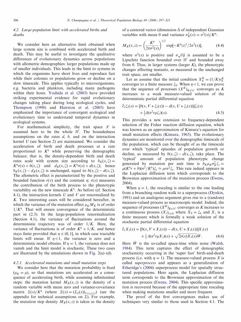
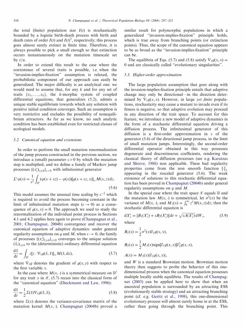
to show that a wide variety of qualitative behaviors obtainsfor different combinations of the mutation parameters s, mand system size K. In each Figs. 1(a)–(d) and 2(a)–(d), theupper panel displays the distribution of trait values in thepopulation at any time and the lower panel displays thedynamics of the total population size, I!t#.

These simulations hint at the different mathematicalapproximations that we establish in Sections 4 and 5.Fig. 1(a)–(c) represent the individual-based process !nt; I!t##with fixed m and s, and with an increasing system size K. As Kincreases, the fluctuations of the population size I!t# (lowerpanels) are strongly reduced, which suggests the existence of a

ARTICLE IN PRESS

Fig. 1. Numerical simulations of trait distributions (upper panels, darker is higher frequency) and population size (lower panels). The initial population ismonomorphic with trait value 1:2 and contains K individuals. (a–c) Qualitative effect of increasing system size (measured by parameter K). (d) Largesystem size and very small mutation probability !m#. Running time was chosen so that similar ranges of trait values were spanned by all simulatedevolutionary trajectories: (a) m $ 0:03, K $ 100, s $ 0:1; (b) m $ 0:03, K $ 3000, s $ 0:1; (c) m $ 0:03, K $ 100 000, s $ 0:1; (d) m $ 0:00001, K $ 3000,s $ 0:1.

N. Champagnat et al. / Theoretical Population Biology 69 (2006) 297–321302

deterministic limit; and the support of the measure nt (upperpanels) spreads over the trait space, which suggests theexistence of a density for the limit measure (see Section 4.1).Fig. 1(d) illustrates the dynamics of the population on a long

timescale, when the mutation probability m is very small. Aqualitatively different phenomenon appears: the populationremains almost monomorphic and the trait evolves accordingto a jump process, obtained in Section 5.

ARTICLE IN PRESS

Fig. 2. Numerical simulations of trait distribution (upper panels, darker is higher frequency) and population size (lower panels) for accelerated birth anddeath and concurrently increased system size. Parameter Z (between 0 and 1) relates the acceleration of demographic turnover and the increase of systemsize. (a) Rescaling mutation step. (b) Rescaling mutation probability. (c–d) Rescaling mutation step in the limit case Z $ 1; two samples for the samepopulation. The initial population is monomorphic with trait value 1:2 and contains K individuals: (a) m $ 0:3, K $ 10 000, s $ 0:3=KZ=2, Z $ 0:5; (b)m $ 0:1=KZ, K $ 10 000, s $ 0:1, Z $ 0:5; (c) m $ 0:3, K $ 10 000, s $ 0:3=KZ=2, Z $ 1; (d) m $ 0:3, K $ 10 000, s $ 0:3=KZ=2, Z $ 1.

N. Champagnat et al. / Theoretical Population Biology 69 (2006) 297–321 303

In Fig. 2, the underlying model involves accelerating thebirth and death processes along with increasing system size,as if the population were made up of a larger number ofsmaller individuals, reproducing and dying at higher rates(see Section 4.2). Specifically, we take

b!x; z# $ KZ ' b!x# and d!x; z# $ KZ ' d!x# ' z,

where b!x#, d!x#, m!x#, U!x# and M!x; z# are definedas in (2.7). Note that the ‘‘demographic timescale’’ ofpopulation growth, that occurs at rate b!x; z# & d!x; z#, isunchanged.

There is a noticeable qualitative difference betweenFigs. 2(a)–(b), where Z $ 1=2, and Figs. 2(c)–(d), whereZ $ 1. In the latter, we observe strong fluctuations in thepopulation size, early extinction happened in manysimulations (Fig. 2(d)) and the evolutionary pattern isfinely branched, revealing that the stochasticity of birthand death persists and generates a new form of stochas-ticity in the large population limit (see Sections 4.2.1and 4.2.2).

3. Moment equations

Moment equations have been introduced in theoreticalpopulation biology by Bolker and Pacala (1997, 1999) andDieckmann and Law (2000) (referred hereafter as BPDL),following on from the seminal work of Matsuda et al.(1992), as handy analytical models for spatially extendedpopulations. A similar approach has been proposedindependently by McKane and Newman (2004) to modelpopulation dynamics when individual stochastic processesoperate in spatially structured habitats. Hereafter, we usethe analogy between population processes defined on traitspace versus physical space to construct the momentequations of the population evolutionary dynamics. The‘‘philosophy’’ of moment equations is germane to theprinciple of Monte-Carlo methods: computing the meanpath of the point process from a large number ofindependent realizations. (The orthogonal stance, as weshall see in Section 4, is to model the behavior of a singletrajectory while making the initial number of individualsbecome large).

Let us define the deterministic measure E!n# asso-ciated with a random measure n by

RX j!x#E!n#!dx# $

E!RX j!x#n!dx##. Taking expectation in (2.3) and using

E!mt!j## $ 0, one can obtain an equation forRX j!x#E!n#!dx# involving the expectations of integralswith respect to n!dx# or n!dx#n!dy#. This is a complicatedequation involving an unresolved hierarchy of nonlinearterms. Writing an equation for E!n!dx#n!dy## is feasible butyields integrals with respect to n!dx#n!dy#n!dz#, and so on.Whether this approach in general may eventually helpdescribe the population dynamics in the trait space is stillunclear.

Let us consider the case of logistic density dependence(see Section 2.2) where d!x; z# $ d!x# ' a!x#z, b!x; z# $ b!x#and m!x# $ 1. Taking expectations in (2.3) with j , 1

yields:

N!t# $ N!0# 'Z t

0E

Z

X)b!x# & d!x#*ns!dx#

! "#

& E

Z

X+Xa!x#U!x& y#ns!dx#ns!dy#

! "$ds, !3:1#

where N!t# $ E!I!t## is the ‘‘mean’’ population size at timet. The specific case where b, d and a are independent of x,and U is symmetrical (cf. Law et al., 2003), corresponds tothe BPDL model of spatial population dynamics. Eq. (3.1)then recasts into

_N $ !b& d#N & aZ

RlU!r#Ct!dr#, (3.2)

where Ct is defined at any time t as a ‘‘spatial covariancemeasure’’ (sensu BPDL) on Rl , given byZ

RlU!r#Ct!dr# $ E

Z

X+XU!x& y#nt!dx#nt!dy#

! ". (3.3)

A dynamic equation for this covariance measure thenobtains by considering the quantities

RRl U!r#Ct!dr# as

functions f!n# in (2.2), but the equation involves momentsof order 3, which prevents ‘‘closing’’ the model on lower-order variables. Even in the simplest mean-field caseU $ 1, we get

_N!t# $ !b& d#N!t# & aEZ

X+Xnt!dx#nt!dy#

! ". (3.4)

Because of the expectation, the covariance term cannot bewritten as a function of the first-order moment N!t#, and,therefore, Eq. (3.4) does not simplify.Even if there is no constructing a closed equation

satisfied by E!n#, we are able to show, in the general case,the following important qualitative property: if thedeterministic measure E!n0# of the initial population admitsa density p0 with respect to the Lebesgue measure, then forall tX0, the deterministic measure E!nt# of the populationhas a probability density pt. To see this, apply (2.3) toj $ 1A where A has zero Lebesgue measure. Taking ex-pectations then yields E!

RX j!x#nt!dx## $

RA E!nt#!dx# $ 0,

which gives the required result. As a consequence, theexpectation of the total size of the population at time t isN!t# $ E!

RX nt!dx## $

RX pt!x#dx, and pt!x#dx= N!t# gives

the probability of observing one individual at time t in asmall ball centered in x with radius dx. In particular, thisresult implies that, when the initial trait distribution E!n0#has no singularity with respect to the Lebesgue measure,these singularities, such as Dirac masses, can only appearin the limit of infinite time.This has biological implications on how one would

analyze the process of population differentiation andphenotypic ‘‘packing’’ (Berstein et al., 1985). Such apopulation model should not be expected to converge infinite time towards neatly separated phenotypic peaks if theancestral phenotypic distribution is even slightly spreadout as opposed to being entirely concentrated on a setof distinct phenotypes. Thus, the biologically relevant


question that theory may address is not whether packingcan arise from a continuous phenotypic distribution, butrather whether initial differentiation (ancestral phenotypicpeaks) is amplified or buffered by the eco-evolutionaryprocess.

4. Large-population renormalizations of the individual-basedprocess

The moment equation approach outlined above is basedon the idea of averaging a large number of independentrealizations of the population process initiated with a finitenumber of individuals. If K denotes the initial number ofindividuals, taken as a measure of the ‘‘system size’’ sensuMetz et al. (1996), an alternative approach to derivingmacroscopic models is to study the exact process by lettingthat system size become very large and making someappropriate renormalization. Several types of approxima-tions can then be derived, depending on the renormaliza-tion of the process.

For any given system size K, we consider the set ofparameters UK , VK , bK , dK , MK , mK satisfying theprevious hypotheses and being all continuous in theirarguments. Let nKt be the counting measure of thepopulation at time t. We define a renormalized populationprocess !XK

t #tX0 by

XKt $

1

KnKt .

!XKt #tX0 is a measure-valued Markov process. As the

system size K goes to infinity, the interaction kernelsneed be renormalized as UK !x# $ U!x#=K and VK !x# $V !x#=K . A biological interpretation of this renormalizationis that larger systems are made up of smaller individuals,which may be a consequence of a fixed amount of availableresources to be partitioned among individuals. Thus, thebiomass of each individual scales as 1=K , and theinteraction kernels are renormalized in the same way, sothat the interaction terms UK % n and VK % n that affect anyfocal individual stay of the same order of magnitude as thetotal biomass of the population.

Martingale theory allows one to describe the dynamicsof XK as the sum of a deterministic trajectory and arandom fluctuation of zero expectation. The decomposi-tion obtains by equations similar to (2.3) and (2.4), inwhich all coefficients depend on K, and the variance (2.4) ofthe martingale part is also divided by K. Derivingapproximation limits for these two terms leads to thealternative choices of timescales that we present in thissection. In particular, the nature (deterministic or stochas-tic) of the approximation can be determined by studyingthe variance of the random fluctuation term.

4.1. Large-population limit

Let us assume that, as K increases, the initial conditionXK

0 $ !1=K#nK0 converges to a finite deterministic measure

which has a density x0 (when this does not hold, thefollowing convergence results remain valid, but from amathematical viewpoint the limit partial differentialequations and stochastic partial differential equations haveto be understood in a weak measure-valued sense).Moreover, we assume that bK $ b, dK $ d, mK $ m,MK $ M. Thus, the variance of the random fluctuationof XK

t is of order 1=K , and when the system size K becomeslarge, the random fluctuations vanish and the process!XK

t #tX0 converges in law to a deterministic measure withdensity xt satisfying the integro-differential equation withtrait variable x and time variable t:

qtxt!x# $ )!1& m!x##b!x;V % xt!x## & d!x;U % xt!x##*xt!x#

'Z

RlM!y; x& y#m!y#b!y;V % xt!y##xt!y#dy.

!4:1#

This result re-establishes Kimura’s (1965) equation (seealso Burger, 2000 , p. 119, Eq. (1.3)) from microscopicindividual processes, showing that the only biologicalassumption needed to scale up to macroscopic evolution-ary dynamics is that of a large population. Importantly,Eq. (4.1) extends Kimura’s original model to the case offrequency-dependent selection.The convergence of XK to the solution of (4.1) is

illustrated by the simulations shown in Fig. 1(a)–(c). Theproof of this result (adapted from Fournier and Meleard,2004) strongly relies on arguments of tightness in finitemeasure spaces (Roelly, 1986). Desvillettes et al. (2004)suggest to refer to xt as the population ‘‘number density’’;then the quantity n!t# $

RX xt!x#dx can be interpreted as

the ‘‘total population density’’ over the whole trait space.This means that if the population is initially seeded with Kindividuals, Kn!t# approximates the number of individualsalive at time t, all the more closely as K is larger.The case of logistic density-dependence with constant

rates b, d, a leads to an interesting comparison withmoment equations (cf. Section 3). Then (4.1) yields thefollowing equation on n!t#:

_n $ !b& d#n& aZ

X+XU!x& y#xt!x#dxxt!y#dy. (4.2)

In the mean-field case U , 1, the trait x becomescompletely neutral, and the population dynamics are notinfluenced by the mutation distribution anymore—they aredriven simply by the classical logistic equation of popula-tion growth:

_n $ !b& d#n& an2. (4.3)

Comparing (4.3) with the first-moment equation (3.4)emphasizes the ‘‘decorrelative’’ effect of the large systemsize renormalization: in the moment equation model (3.4)that assumes finite population size, the correction termcapturing the effect of correlations of population sizeacross the trait space remains, even if one assumes U , 1.


4.2. Large-population limit with accelerated births anddeaths

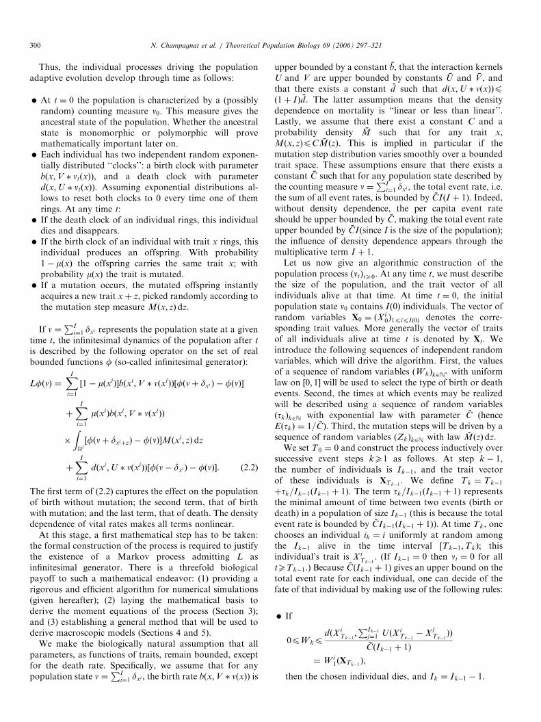
We consider here an alternative limit obtained whenlarge system size is combined with accelerated birth anddeath. This may be useful to investigate the qualitativedifferences of evolutionary dynamics across populationswith allometric demographies: larger populations made upof smaller individuals. This leads in the limit to systems inwhich the organisms have short lives and reproduce fastwhile their colonies or populations grow or decline on aslow timescale. This applies typically to microorganisms,e.g. bacteria and plankton, including many pathogenswithin their hosts. Yoshida et al. (2003) have providedstriking experimental evidence for rapid evolutionarychanges taking place during long ecological cycles, andThompson (1998) and Hairston et al. (2005) haveemphasized the importance of convergent ecological andevolutionary time to understand temporal dynamics inecological systems.

For mathematical simplicity, the trait space X isassumed here to be the whole Rl . The boundednessassumptions on the rates d, b, and on the interactionkernel U (see Section 2) are maintained. We consider theacceleration of birth and death processes at a rateproportional to KZ while preserving the demographicbalance; that is, the density-dependent birth and deathrates scale with system size according to bK !x; z# $KZr!x# ' b!x; z# and dK !x; z# $ KZr!x# ' d!x; z#; hencebK !x; z# & dK !x; z# is unchanged, equal to b!x; z# & d!x; z#.The allometric effect is parameterized by the positive andbounded function r!x# and the constant Z; r!x# measuresthe contribution of the birth process to the phenotypicvariability on the new timescale KZ. As before (cf. Section4.1), the interaction kernels U and V are renormalized byK. Two interesting cases will be considered hereafter, inwhich the variance of the mutation effect mKMK is of order1=KZ. That will ensure convergence of the deterministicpart in (2.3). In the large-population renormalization(Section 4.1), the variance of fluctuations around thedeterministic trajectory was of order 1=K . Here, thevariance of fluctuations is of order KZ + 1=K , and hencestays finite provided that Z 2 !0; 1*, in which case tractablelimits will ensue. If Zo1, the variance is zero and adeterministic model obtains. If Z $ 1, the variance does notvanish and the limit model is stochastic. These two casesare illustrated by the simulations shown in Fig. 2(a)–(d).

4.2.1. Accelerated mutations and small mutation stepsWe consider here that the mutation probability is fixed

!mK $ m#, so that mutations are accelerated as a conse-quence of accelerating birth, while assuming infinitesimalsteps: the mutation kernel MK !x; z# is the density of arandom variable with mean zero and variance-covariancematrix S!x#=KZ (where S!x# $ !Sij!x##1pi;jpl) (see theappendix for technical assumptions on S). For example,the mutation step density MK !x; z# is taken as the density

of a centered vector (dimension l) of independent Gaussianvariables with mean 0 and variance s2K !x# $ s2!x#=KZ:

MK !x; z# $KZ

2ps2!x#

! "l=2

exp)&KZjzj2=2s2!x#*, (4.4)

where s2!x# is positive and s%%%%%rm

pis assumed to be a

Lipschitz function bounded over Rl and bounded awayfrom 0. Thus, in larger systems (larger K), the phenotypicchanges affecting mutants, as measured in the unchangedtrait space, are smaller.Let us assume that the initial condition XK

0 $ !1=K#nK0converges to a finite measure x0. When Zo1, we can provethat the sequence of processes !XK #K2N% converges as Kincreases to a weak measure-valued solution of thedeterministic partial differential equation

qtxt!x# $ )b!x;V % xt!x## & d!x;U % xt!x##*xt!x#

' 12D!s

2rmxt#!x#. !4:5#

This provides a new extension to frequency-dependentselection of the Fisher reaction–diffusion equation, whichwas known as an approximation of Kimura’s equation forsmall mutation effects (Kimura, 1965). The evolutionarydynamics are monitored over the demographic timescale ofthe population, which can be thought of as the timescaleover which ‘typical’ episodes of population growth ordecline, as measured by b!x; z# & d!x; z#, take place. The‘typical’ amount of population phenotypic changegenerated by mutation per unit time is bKmKs2Kxt $m!KZr' b#!s2=KZ#xt - mrs2xt. This rate indeed appears inthe Laplacian diffusion term which corresponds to theBrownian approximation of the mutation process (Ewens,2004).When Z $ 1, the rescaling is similar to the one leading

from a branching random walk to a superprocess (Dynkin,1991) and an analogous argument gives rise to a (random)measure-valued process as macroscopic model. Indeed, thesequence of processes !XK #K2N% converges as K increases toa continuous process !Xt#tX0 where X 0 $ x0 and Xt is afinite measure which is formally a weak solution of thestochastic partial differential equation

qtX t!x# $ )b!x;V % Xt!x## & d!x;U % Xt!x##*Xt!x#

' 12D!s

2rmXt#!x# '%%%%%%%%%%%%%%%%%%%%%%2r!x#Xt!x#

p_W . !4:6#

Here _W is the so-called space-time white noise (Walsh,1984). This term captures the effect of demographicstochasticity occurring in the ‘super fast’ birth-and-deathprocess (i.e. with Z $ 1). The measure-valued process X iscalled superprocess and appears as a generalization ofEtheridge’s (2004) superprocess model for spatially struc-tured populations. Here again, the Laplacian diffusionterm corresponds to the Brownian approximation of themutation process (Ewens, 2004). This specific approxima-tion is recovered because of the appropriate time rescalingwhen making mutations smaller and more frequent.The proof of the first convergences makes use of

techniques very similar to those used in Section 4.1. The


proof of the second statement requires additional resultsthat are specific to superprocesses (Evans and Perkins,1994) in order to establish uniqueness of the limit process.Both proofs are expounded in the appendix, for the generalcase of the mutation kernel with covariance matrixS!x#=KZ, and the corresponding general results can bestated as follows. When Zo1, the process XK converges tothe solution of the following deterministic reaction–diffu-sion equation:


'1

2

X

1pi;jpl

q2ij!rmSijxt#!x#, !4:7#

where q2ij f denotes the second-order partial derivative of fwith respect to xi and xj !x $ !x1; . . . ; xd##. When Z $ 1,the limit is the following stochastic partial differentialequation:


'1

2

X

1pi;jpl

q2ij!rmSijX t#!x# '%%%%%%%%%%%%%%%%%%%%%%2r!x#Xt!x#

p_W .

!4:8#

The simulations displayed in Fig. 2(c)–(d), comparedwith Fig. 2(a), give a flavor of the complexity of thedynamics that the individual process can generate underthe conditions leading to the superprocess models (4.6) or(4.8). Two distinctive features are the fine branchingstructure of the evolutionary pattern, and the widefluctuations in population size that occur in parallel. Infact, replicated simulations show that the system oftenundergo rapid extinction (Fig. 2(d)). The results of oursimulations suggest that the super fast timescale involvedhere is a general cause for complex population dynamics onthe demographic timescale and for extinction driven by thejoint ecological and evolutionary processes, which isgermane to the phenomenon of evolutionary suicidedescribed in adaptive dynamics theory (Dercole et al.,2002; Ferriere et al., 2002; Dieckmann and Ferriere, 2004);this may be largely independent of the ecological details ofthe system. This conjecture is supported by the mathema-tical proof of almost sure extinction obtained by Etheridge(2004) in her study of a related superprocess describingspatial population dynamics.

4.2.2. Rare mutationsHere, the mutation step densityM is kept constant, while

the mutation rate is decelerated proportionally to 1=KZ:mK $ m=KZ. Thus only births without mutation areaccelerated. As in Section 4.2.1, the macroscopic modelkeeps track of the phenotypic distribution over thepopulation demographic timescale, which coincides herewith the mutation timescale. Again, the limit model can bedeterministic or stochastic, depending on whether theallometric parameter Z is less than 1 or equal to 1,respectively.

Let us assume that the initial condition XK0 $ !1=K#nK0

converges to the finite measure with density x0. When Zo1,the sequence of processes !XK #K2N% converges, as Kincreases, to a measure-valued process with density xtsolution of the following deterministic nonlinear integro-differential equation:


'Z

RlM!y; x& y#m!y#r!y#xt!y#dy. !4:9#

This equation is similar to (4.1), where the allometric effectrate r appears in lieu of the birth rate b in the mutationterm; this is because the per capita mutation rate is equal tomKbK $ !m=KZ#!KZr' b# - mr, while the mutation stepdensity is kept constant. Simulations of the individualprocess under the conditions leading to this model areshown in Fig. 2(b). When Z $ 1, we show, by argumentssimilar to those involved in Section 4.2.1, that the limitmodel is a measure-valued (random) process, whichobtains as weak solution of the stochastic integro-differential equation


'Z

RlM!y;x& y#m!y#r!y#Xt!dy#

'%%%%%%%%%%%%%%%%%%%%%%2r!x#Xt!x#

p_W , !4:10#

where _W is a space-time white noise.Eqs. (4.9) and (4.10) are obtained in a limit of rare

mutations, with accelerated birth and death, on a timescalesuch that the order of magnitude of the individual mutationrate remains constant. In the next section, we study thebehavior of the population process in a limit of raremutations and accelerated birth and death, on an evenlonger timescale, such that the order of magnitude of thetotal mutation rate in the population remains constant.This assumption of extremely rare mutations leads to adifferent class of stochastic models which will provide adescription of the population dynamics on a slow evolu-tionary timescale.

5. Renormalization of the monomorphic process andadaptive dynamics

Metz et al. (1996) have introduced an asymptotic of raremutations to approximate the process of adaptive evolu-tion with a monomorphic jump process. The jump processdescribes evolutionary trajectories as trait substitutionsequences developing over the timescale of mutations.Dieckmann and Law (1996) have further introducedingenious heuristics to achieve a deterministic approxima-tion for the jump process, solution to the so-calledcanonical equation of adaptive dynamics. Metz et al.’snotion of trait substitution sequences and Dieckmann andLaw’s canonical equation form the core of the currenttheory of adaptive dynamics. In this section, we present arigorous derivation of the stochastic trait substitution


sequence jump process from the individual-based modelinitiated with a monomorphic ancestral condition. Ourderivation emphasizes how the mutation scaling shouldcompare to the system size (K) in order to obtain thecorrect timescale separation between mutant invasionevents (taking place on a short timescale) and mutationoccurrences (defining the evolutionary timescale). Next werecover a generalized canonical equation as an approxima-tion of the jump process in an asymptotic of smallmutation steps. We also propose a diffusion approximationof the jump process which allows one to study the timescaleon which a change of basin of attraction for anevolutionary trajectory can occur, providing insights intopatterns of macroevolutionary change (for related theore-tical considerations, see Rand and Wilson, 1993).

5.1. Jump process construction from IBM

The mathematically rigorous construction of the jumpprocess from the individual-based model requires that wefirst study the behavior of a monomorphic population inthe absence of mutation, and next the behavior of adimorphic population, involving competition, after amutation has occurred. In the limit of large system size!K ! 1# without mutation !m , 0#, with only trait xpresent at time t $ 0, we have XK

0 $ nK0 !x#dx and XKt $

nKt !x#dx for any time t. Using the same scaling parametersas in Section 4.1 (UK $ U=K , VK $ V=K , bK and dK

independent of K), the convergence result stated thereintells us that nKt !x# approaches nt!x# when K becomes large,and Eq. (4.1) (in its weak form) becomes

d

dtnt!x# $ r1!x; nt!x##nt!x# (5.1)

where r1!x; nt!x## $ b!x;V !0#nt!x## & d!x;U!0#nt!x##. Wewill assume that r1!x; 0#40, that r1!x; n# ! &1 whenn ! '1, and that, for any trait x, this differentialequation possesses a unique positive equilibrium n!x#,necessarily satisfying b!x;V !0#n!x## $ d!x;U!0#n!x##.Then, it takes only elementary calculus to prove that anysolution to (5.1) with positive initial condition converges ton!x#. In the case of linear logistic density-dependenceintroduced in Section 2.2 (b!x; z# $ b!x# and d!x; z# $d!x# ' a!x#z), the equilibrium monomorphic density n!x#is !b!x# & d!x##=a!x#U!0#.

When the population is dimorphic with traits x and y,i.e. when XK

0 $ nK0 !x#dx ' nK0 !y#dy, we can define nt!x# andnt!y# for any t as before. Then xt $ nt!x#dx ' nt!y#dysatisfies Eq. (4.1), which recast into the following systemof coupled ordinary differential equations:

d

dtnt!x# $ r2!x; y; nt!x#; nt!y##nt!x#,

d

dtnt!y# $ r2!y; x; nt!y#; nt!x##nt!y#, !5:2#

where r2!x; y; n; n0# $ b!x;V !0#n'V !x&y#n0#& d!x;U!0#n'U!x& y#n0#. Note that r2!x; y; n; 0# $ r1!x; n#. The system

(5.2) possesses two (non-trivial) equilibria on the boundaryof R' + R', !n!x#; 0# and !0; n!y##, which must be stable inthe horizontal and vertical direction, respectively. We thenstate as a rule that ‘‘y invades x’’ if the equilibrium !n!x#; 0#of (5.2) is unstable in the vertical direction; this can beshown to occur if r2!y; x; 0; n!x##40 (Ferriere and Gatto,1995; Geritz et al., 2002; Rinaldi and Scheffer, 2000). Wefurther say that ‘‘invasion of x by y implies fixation’’ ifr2!y;x; 0; n!x##40 entails that all orbits of the dynamicalsystem (5.2) issued from sufficiently small perturbations ofthe equilibrium !n!x#; 0# in the positive orthant converge to!0; n!y##. Our construction requires that this property holdsfor almost any mutant trait y borne out from x. Geritzet al. (2002) and Geritz (2004) have actually proved thatthis is true for general models when the mutant trait is closeto the resident and the resident is sufficiently far fromspecial trait values corresponding to branching points orextinction points of the trait space X. From a biologicalviewpoint, the quantity r2!y;x; 0; n!x## is the fitness ofmutant y in a resident population of trait x at equilibrium(Metz et al., 1992), which we will hereafter denote by f !y;x#and refer to as the fitness function. Note that the fitnessfunction f satisfies the usual property that f !x;x# $ 0 forany trait value x.The heuristics of trait substitution sequence models

(Metz et al., 1996) assume that a monomorphic populationreaches its ecological (deterministic) equilibrium before thefirst mutation occurs. As a mutant arises, it competes withthe resident trait, and sufficient time is given to theecological interaction for sorting out the winner before anew mutant appears. In the simplest case, only one traitsurvives: either the mutant dies out (due to stochasticity orselective inferiority), or it replaces the resident trait (due tostochasticity or selective superiority). Therefore, on a longtimescale, the evolutionary dynamics can be described as asuccession of ‘‘mutation-invasion’’ events corresponding tojumps in the trait space.These heuristics raise conflicting demands on the

mutation rate that only a full mathematical treatmentcan resolve. First, mutation events should be rare enoughso that the next mutant is unlikely to appear until theprevious mutant’s fixation or extinction is settled. Second,mutation events should be frequent enough, so that the nextmutation is not delayed beyond the time when the residentpopulation size is likely to have stochastically drifted awayfrom its equilibrium. Large deviation theory (Dembo andZeitouni, 1993) and results on Galton-Watson processes canbe used to determine the correct mutation timescale for whichboth conditions are satisfied. The mathematical work isreported in Champagnat (2004a), and the end result ofbiological interest is that, if the mutation probability is takenas mK !x# $ uKm!x#, where uK converges to zero when K goesto infinity, then the mutation probability and the system sizeshould scale according to

e&CK5uK51

K logKfor any C40. (5.3)


Eq. (5.3) implies in particular that KuK tends to 0 as Ktends to infinity; therefore, for each time t, the time changet=KuK represents a long time scaling. This slow timescale isthat of the mutation process: the population size is of theorder of K, and the per capita mutation rate is proportionalto uK , hence the population mutation rate is of the order ofKuK . Conditions (5.3) may be rewritten as

logK5t

KuK5eCK for any t;C40,

and obtains because logK is the typical time of growth andstabilization of a successful mutant, and exp!CK# is thetypical time over which the resident population is likely todrift stochastically away from deterministic equilibrium(problem of exit from a domain, Freidlin and Wentzel,1984).

Under assumption (5.3), the method developed inChampagnat (2004a) can be adapted to prove that, as thesystem size K becomes large, the process XK

t=KuK$

!1=K#nKt=KuK converges, when the initial distribution ismonomorphic with trait x, to the process n!Yt#dYt inwhich the population is at any time monomorphic.The time process involved, !Yt#tX0, is Markovian andsatisfies Y 0 $ x. This is a jump process with infinitesimalgenerator L given, for all bounded measurable functionj:X ! R, by

Lj!x# $Z

Rl!j!x' z# & j!x##)g!x' z;x#*'M!x; z#dz

(5.4)

where

g!y;x# $ m!x#b!x;V !0#n!x##n!x#f !y;x#

b!y;V !y& x#n!x##(5.5)

()z*' denotes the positive part: )z*' $ 0 if zp0; )z*' $ zif z40). The generator’s form (5.4) means thatthe process Yt jumps from state x with rate R!x# $RRl )g!x' z; x#*'M!x; z#dz to the new state x' z, where zfollows the law )g!x' z;x#*'M!x; z#dz=R!x#. The simula-tion shown in Fig. 1(d) illustrates this convergence resultand the behavior of the process !Yt#tX0.

The expression for g given by Eq. (5.5) can be under-stood as follows. When the population is monomorphicwith trait x, its density reaches a given neighborhood of itsequilibrium n!x# in finite time, i.e. within an infinitesimaltime with respect to the timescale of mutation; this can beshown by using results on stochastic comparison between!nKt # and logistic birth-and-death processes. Then, thepopulation size being close to n!x#, the populationmutation rate is close to uKm!x#b!x;V !0#n!x##Kn!x#. There-fore, on the mutation timescale, the mutation rate is givenby m!x#b!x;V !0#n!x##n!x#, which yields one part of (5.5).The other part deals with the invasion of a mutant trait y,which can be divided into three phases (Fig. 3), as is doneclassically by population geneticists dealing with selectivesweeps (Kaplan et al., 1989; Durrett and Schweinsberg,2004). Initially, there is only one mutant individual; the

population it spawns may go extinct quickly even if itsfitness f !y; x# is positive, due to demographic stochasticity.To estimate the probability of such early extinction, wecompare the number of mutant individuals, as long as it issmall with respect to the resident population size, withGalton–Watson processes, with constant birth and deathrates. This first phase ends when the mutant density reachesa fixed small level g and corresponds in Fig. 3 to the timeinterval )0; t1*. Here, the mutant birth rate is close tob!y;V !y& x#n!x##, and the mutant death rate is close tod!y;U!y& x#n!x##. The probability of survival of aGalton–Watson process with these parameters is givenclassically as )f !y; x#*'=b!y;V !y& x#n!x##, which yields thesecond part of (5.5). If invasion occurs, which is possibleonly if f !y;x#40, the resident and mutant densities getclose to the solution of Eq. (5.2), represented by the dottedcurves between t1 and t2 in Fig. 3; this is phase 2. Since weassume that ‘‘invasion implies fixation’’, the residentdensity converges to 0 and reaches level g in boundedtime. The third phase (between times t2 and t3 in Fig. 3) isanalyzed by means of a comparison argument between thenumber of resident individuals and a Galton–Watsonprocess similar to the previous one, which allows us toprove that the resident population goes extinct ininfinitesimal time with respect to the mutation timescale.These arguments can be expounded formally by adaptingthe method of Champagnat (2004a). The times t1 and t3 & t2are of the order of logK , while t2 & t1 only depends on g.The mathematical derivation of the jump process model

(5.4) and (5.5) emphasizes that the rare-mutation andlarge-population limits must be taken simultaneously if oneis to model evolutionary dynamics as a stochastic traitsubstitution sequence. On the other hand, the largepopulation limit by itself can only yield the deterministicmodel (4.1) (generalized Kimura’s equation). On the otherhand, the dynamics of a finite population on the mutationtimescale are trivial under the rare mutation scenario: thepopulation goes immediately extinct almost surely on thattimescale. This follows from the fact that the individual-based process n (cf. Section 2.1) that drives the dynamics of

ARTICLE IN PRESS

Fig. 3. The three phases of the invasion and fixation of a mutant trait y ina monomorphic population with trait x. Plain curves represent the residentand mutant densities nKt !x# and nKt !y#, respectively. Dotted curvesrepresent the solution of Eq. (5.2) with initial state n0!x# $ n!x# andn0!y# $ e.

N. Champagnat et al. / Theoretical Population Biology 69 (2006) 297–321 309

the total (finite) population size I!t# is stochasticallybounded by a logistic birth-death process with birth anddeath rates of order I!t# and I!t#2, respectively; this processgoes almost surely extinct in finite time. Therefore, it isalways possible to pick u small enough so that extinctionoccurs instantaneously on the mutation timescale setby t=u.

In order to extend this result to the case where thecoexistence of several traits is possible, i.e. when the‘‘invasion-implies-fixation’’ assumption is relaxed, theprobabilistic component of our approach can easily begeneralized. The major difficulty is an analytical one: wewould need to assume that, for any k and for any set oftraits fx1; . . . ;xkg, the k-morphic system of coupleddifferential equations, that generalizes (5.2), admits aunique stable equilibrium towards which any solution withpositive initial condition converges. Such an assumption isvery restrictive and excludes the possibility of nonequili-brium attractors. As far as we know, no such analyticcondition has been established even for restricted classes ofecological models.

5.2. Canonical equation and extensions

In order to perform the small mutation renormalizationof the jump process constructed in the previous section, weintroduce a (small) parameter e40 by which the mutationstep is multiplied, and we define a family of Markov jumpprocesses f!xet#tX0ge40 with infinitesimal generator

Lej!x# $1

e2

Z

Rl!j!x' ez# & j!x##)g!x' ez;x#*'M!x; z#dz.

(5.6)

This model assumes the unusual time scaling by e&2 whichis required to avoid the process becoming constant in thelimit of infinitesimal mutation steps !e ! 0# as a conse-quence of g!x;x# $ 0. The approach we used to study therenormalization of the individual point process in Sections4.1 and 4.2 applies here again to prove (Champagnat et al.,2001; Champagnat, 2004b) convergence and recover thecanonical equation of adaptive dynamics: under generalregularity assumptions on g andM, when e ! 0, the familyof processes f!xet#tX0geX0 converges to the unique solution! ~xt#tX0 to the (deterministic) ordinary differential equation

d ~xdt

$Z

Rlz)z " r1g! ~x; ~x#*'M! ~x;dz#, (5.7)

where r1g denotes the gradient of g!x; y# with respect tothe first variable x.

In the case where M!x; "# is a symmetrical measure on Rl

for any trait x in X, (5.7) recast into the classical form ofthe ‘‘canonical equation’’ (Dieckmann and Law, 1996):

d ~xdt

$1

2S! ~x#r1g! ~x; ~x#, (5.8)

where S!x# denotes the variance-covariance matrix of themutation kernel M!x; "#. Champagnat (2004b) proved a

similar result for polymorphic populations in which ageneralized ‘‘invasion-implies-fixation’’ principle holds,which is true away from branching points (or extinctionpoints). Thus, the scope of the canonical equation appearsto be as broad as the ‘‘invasion-implies-fixation’’ principlecan be.The equilibria of Eqs. (5.7) and (5.8) satisfy r1g!x; x# $

0 and are classically called ‘‘evolutionary singularities’’.

5.3. Higher-order approximation

The large population assumption that goes along withthe invasion-implies-fixation principle entails that adaptivechange may only be directional—in the direction deter-mined by r1g!x;x#. However, in large yet finite popula-tions, stochasticity may cause a mutant to invade even if itsfitness is negative, so that adaptive evolution may proceedin any direction of the trait space. To account for thisfeature, we introduce a new model of adaptive dynamics inthe form of a stochastic differential equation driving adiffusion process. The infinitesimal generator of thisdiffusion is a first-order approximation in e of thegenerator (5.6) of the directional jump process, in the limitof small mutation jumps. Interestingly, the second-orderdifferential operator obtained in this way possessesdegenerate and discontinuous coefficients, rendering theclassical theory of diffusion processes (see e.g. Karatzasand Shreve, 1988) non applicable. These bad regularityproperties come from the non smooth function )"*'appearing in the rescaled generator (5.6). The weakexistence of solutions to this stochastic differential equa-tion has been proved in Champagnat (2004b) under generalregularity assumptions on g and M.In the special case where the trait space X equals R and

the mutation law M!x; "# is symmetrical, let s2!x# be thevariance of M!x; "#, and M3!x# $

R10 z3M!x; z#dz; then the

stochastic differential equation is

dX et $ )B1!X e

t# ' eB2!X et#*dt'

%%%%%%%%%%%%%%%eA!X e

t#p

dWt, (5.9)

where

B1!x# $1

2s2!x#q1g!x;x#,

B2!x# $1

2M3!x#sign)q1g!x;x#*q21g!x; x#,

A!x# $ M3!x#jq1g!x; x#j,

and W is a standard Brownian motion. Brownian motiontheory then suggests to probe the behavior of this one-dimensional process when the canonical equation possessesmultiple locally stable equilibria. The results of Champag-nat (2003) can be applied here to show that when anancestral population is surrounded by an attracting ESS(evolutionarily stable strategy) and an attracting branchingpoint (cf. e.g. Geritz et al., 1998), this one-dimensionalevolutionary process will almost surely home in at the ESS,rather than going through the branching point. This


mathematical result substantiates the numerical observa-tion that branching is usually a very slow phenomenon;thus, when mutations steps are small, branching points areso difficult to reach as to leave time for the system tostabilize at an ESS if there is one within mutational reach.Therefore, to ensure that a population with unknownmonomorphic ancestral state undergoes evolutionarybranching, all of the attracting evolutionary singularitiesshould be branching points.

In general, the issue of evolutionary dynamics driftingaway from trajectories predicted by the canonical equationcan be investigated by considering the asymptotic of theprobability of ‘rare events’ for the sample paths of thediffusion. By ‘rare events’ we mean diffusion paths driftingfar away from the canonical equation. The probability ofsuch rare events is governed by a large deviation principle(Wentzel, 1976a,b; Freidlin and Wentzel, 1984): when egoes to 0, the probability that the sample path of thediffusion process is close to a given rare path j decreasesexponentially to 0 with rate I!j#, where the ‘rate function’ Ican be expressed in terms of the parameters of thediffusion. The difficulty lies in the fact that the diffusioncoefficient A is null at the evolutionary singularities andthat the drift term B2 is discontinuous at the same points,and the same problem arises for any value of the dimensionl of the trait space. The large deviation principle has beenobtained by Champagnat (2003) for any value of the traitspace dimension, and implies in particular that the paths ofX e

t converge in probability to the solution of the canonicalequation (5.8) when e goes to 0.

This result can be used to study the long-time behaviorof the diffusion process when there are multiple attractiveevolutionary singularities and the dimension of the traitspace X is 2 or greater. Let us introduce the ‘quasi-potential’ H!x; y# as the minimum of the rate function Iover all the trajectories linking x to y. When e is small, themost likely path followed by the diffusion when exiting thebasin of attraction G of some evolutionary singularity x%, isthe one minimizing the rate function I over all thetrajectories linking x% to the boundary of G. Therefore,the time needed to exit G can be shown (Champagnat,2003) to be of the order of or greater than exp)H=e* forsmall e, where H is the minimum of H!x%; y# over all the yin the boundary of G. Moreover, the exit event occurs withprobability converging to 1 in any neighborhood of specialpoints of the basin’s boundary where the quasi-potentialH!x%; "# is minimum, so that one can predict the next basinof attraction visited by the diffusion. From a biologicalstandpoint, this result provides a quantitative tool foranalyzing the macroevolutionary notion of punctuatedequilibria (Rand and Wilson, 1993; Stanley, 1979). Themodel generally predicts that the order of magnitude of thetime spent in the neighborhood of evolutionary equilibria,between rapid evolutionary moves, is the exponential of theinverse of the mutation step standard deviation. Thistheory also predicts the sequence order of evolutionarysingularities (equilibria or general attractors) that the

evolutionary process is most likely to visit (Freidlin andWentzel, 1984).

6. Discussion and conclusion

Martingale and large deviation theories provided us withthe new probabilistic tools which were necessary forderiving and unifying models of evolutionary dynamicsfrom stochastic nonlinear processes operating at theindividual level. Different macroscopic models obtaindepending on the renormalizations applied to the stochas-tic individual-based model. Hereafter we review thedifferent models thus obtained and highlight how someof them relate to models previously known in quantitativegenetics and evolutionary ecology. Then we review thebiological insights that one can gain from the veryconstruction of these models. Finally, we outline somepromising directions for the analysis and further extensionsof these models.

6.1. Unifying macroscopic models of evolutionary dynamics

A Monte-Carlo approach yields a hierarchy of equationsdescribing the dynamics of the moments of populationnumber in trait space. A similar approach has been takenheuristically by Bolker and Pacala (1997, 1999), Dieck-mann and Law (2000) and McKane and Newman (2004) toconstruct macroscopic models of population dynamics inphysical (geographic) space while accounting for individualdispersal. Our mathematical derivation sheds light on thestructural features of the model which makes the problemof moment closure so challenging, especially the fact that,in general, the covariance measure may not have a density.Alternatively to the Monte-Carlo approach, various

macroscopic models obtain for different timescale separa-tions, under the common assumption of the system sizebeing large. The large-population limit by itself yields ageneralization to frequency- and density-dependent selec-tion scenarios of Kimura’s (1965) continuum-of-allelesmodel (a nonlinear integro-differential equation). Theassumption of small mutational effects, under whichKimura derived a diffusion approximation of his model,can be made while simultaneously accelerating the in-dividual process of birth and death. This leads toseparating the timescale of individual birth and death(assumed to be fast) from the timescale of populationdemography (over which significant population growth ordecline occurs). This timescale separation may be mostappropriate to study the interplay of ecological andevolutionary processes in microorganisms (Turchin, 2003;MacLean, 2005), including pathogens in which the concernof rapid evolution urges the need for appropriate modellingtools. The resulting model is a reaction–diffusion equationsimilar to Kimura’s approximation and generalized tofrequency- and density-dependent selection. Interestingly,the scaling exponent (Z, between 0 and 1) which defines theproper acceleration of birth and death as the population


size is made larger, has no effect on the macroscopicdynamics, except when Z $ 1 which corresponds tomaximum birth-death acceleration. In this case, themacroscopic model is structurally different, as it takes theform of a stochastic partial differential equation. Simula-tions of the individual process in this case (Fig. 2(c)–(d))show that the evolutionary dynamics has a finely branched,fractal structure (we suspect that its Hausdorff dimensionis between 1 and 2); the population displays wildfluctuations in total size, and faces a high risk of rapidextinction—a phenomenon akin to evolutionary suicide(Dieckmann and Ferriere, 2004).

The separation of the (fast) individual birth and deathtimescale and slow population demography can also beassumed under a rare- (rather than small-) mutationscenario. A model similar to Kimura’s integro-differentialequation obtains, but in which the ‘loss’ of individualbirths with any given trait due to mutation is not apparent.This reflects the fact that when the birth process is fastwhile the mutation probability becomes infinitesimal, thechange in the frequency of any given trait due to mutationis caused predominantly by ‘incoming’ mutants born fromprogenitors carrying other trait values. As before, themacroscopic model does not depend upon the birth-deathacceleration exponent Z, except when birth and death aremade maximally fast !Z $ 1#, in which case the model is astochastic nonlinear integro-differential equation.

The previous limits make the timescales of ‘typical’mutation steps and ‘typical’ variation in population sizecoincide. An alternative approach is to assume thatvariation in population size occurs on a fast timescalecompared to the timescale of mutation steps. This is thebasis for modelling evolutionary dynamics as stochastictrait substitution sequences (Metz et al., 1996), whichunderlies the adaptive dynamics approach. We show thatsuch trait substitution sequences are trajectories of a jumpprocess which obtains under the assumption of an ancestralpopulation being monomorphic. Our approach clearlyisolates and solves the two key issues raised by theheuristics of the original derivation of adaptive dynamicsmodels (Dieckmann and Law, 1996). One issue is under-scored by the construction of the infinitesimal generator ofthe jump process. In Dieckmann–Law’s heuristics, thepopulation growth of a mutant is described by aGalton–Watson branching process, which appropriatelyassumes that the mutant population is finite; at the sametime, however, the mutant branching process is parameter-ized by the density of the resident population which isassumed to be infinitely large. Resolving the tensionbetween these conflicting assumptions requires that thewhole system be regarded as finite, which then raises theissue that the resident population, being large yet finite,may stochastically drift away from the deterministicequilibrium predicted by the infinitely large populationlimit. The issue is taken care of by using large deviationtheory to specify the appropriate mutation timescale overwhich this is unlikely to happen.

The second issue with the canonical equation heuristics(Dieckmann and Law, 1996) was the notion that thesolution to the equation should describe the mean traitvalue in the population for small mutation steps. Ourderivation shows that, in fact, the canonical equationdrives the exact path of the jump process in the limit ofinfinitesimal mutation steps, which provides a mathema-tical justification for Dieckmann and Law’s ‘‘mean path’’interpretation. Our derivation further implies that thecanonical equation orbits describe population change on a‘super long’ timescale: firstly, time t is scaled as t=KuKwhere uK $ o!1=K# is the order of magnitude of mutationprobability (rare mutation assumption) and secondly, timeis scaled by 1=e2 where e is the order of magnitude ofmutation steps. This rescaling may be taken as a formaldefinition for the notion of a ‘macroevolutionary’ time-scale.

6.2. Biological insights from the process of modelconstruction

A general conclusion that emerges from this work is thathow timescales of individual processes compare to eachother can have a major impact on the structure ofmacroscopic models (integro-differential equations versusreaction–diffusion equations, deterministic versus stochas-tic), hence on the evolutionary dynamics predicted by thesemodels. This was lucidly anticipated by Barton andPolechova (2005) in a commentary of the limitations ofadaptive dynamics models, and is herein illustrated bysimulations (Figs. 1 and 2), that hint at a whole array ofstrikingly different qualitative behaviors:

( In large populations, the process of diversification isfaster (compare Figs. 1(a) and (b)) and can turn fromgradual (Fig. 1(b)) to discontinuous and step-wise(Fig. 1(c)).

( For a given system size, extreme mutation rarity changesthe prediction of diversifying dynamics in which bothstabilizing selection and disruptive selection play strongroles (Fig. 1(b)), to a pattern dominated by stabilizingselection in which the population remains essentiallymonomorphic (Fig. 1(d)).

( When rare mutations occur in a large population ofindividuals reproducing and dying at high rates,phenotypic diversification occurs, although more slowlyand to a lesser extent (Fig. 2(b)).

( In a large population of individuals reproducing anddying fast, mutations that are small rather than rare willcause a discontinuous pattern of diversification similarto Fig. 1(c), see Fig. 2(a). However, as mutationparameters m and s become smaller, the tendency fordiversification is strongly limited, which demonstratesthat the timescale of diversification is highly sensitive tothe mutation pattern.

( However, maximal acceleration of birth and deathassociated with minimal mutation steps in large systems


generates yet another type of evolutionary dynamics,involving a high rate of diversification of the populationinto fine phenotypic clusters combined with a high rateof extinction of these clusters; the resulting evolutionarypattern has a remarkable fractal structure, as seen inFig. 2(c). In particular, the pattern shown in that figuresuggests that there might exist a general scaling relation-ship between the width of phenotypic clusters and theirrate of extinction.

A simplistic aspect of our models resides in the absenceof physiological, social or environmental structure: theindividual life history is reduced to the simplest possiblebirth and death process. Although this simplifyingassumption narrows down the scope of our theory, it hasthe merit of making the models thus obtained directlycomparable to the classical models of population genetics,quantitative genetics and adaptive dynamics, which werederived under a similar assumption. Much generality,however, is kept in our treatment of density dependenceand in the way adaptive traits influence individualprocesses.

When considering the acceleration of birth and death,the most general case we could handle involved rescalingthe birth rate as

bK $ b x;U

K% n

! "' r!x#KZ (6.1)

(and similar rescaling for the death rate). This relationshipbetween birth and system size lends itself to interpretationwithin the context of allometries and life-history scaling(Calder, 1984; Charnov, 1993; Brown et al., 2004). Eq. (6.1)means that for large system size, density dependence iseffectively ‘felt’ by any individual as a consequence of thelarge number of competitors (rather than the individualeffect of each competitor), which suggest that large systemsize implicitly comes along with individuals being small.Let us introduce the notion of a taxonomic size’ (or mass)m to express such a relationship more precisely. One canthink of m as a macroscopic parameter (characteristic of aspecies or taxonomic group) which is fixed on themicroevolutionary scale over which x can change adap-tively. It is known (Damuth, 1987; Belgrano et al., 2002)that the system size, K, scales with the &3=4 power of(taxonomic) body mass, m. Thus, across the range of largesystem sizes, i.e., small organisms, the birth rate given byEq. (6.1) is approximately equal to r!x#m&3Z=4. Thus, thismodel makes it possible to explore the adaptive evolutionof the intercept, r!x#, (at least over a range of sufficientlysmall mass) of the power law that scales birth rate withbody mass—an issue currently attracting much attentionfrom life-history biologists (Economo et al., 2005;McCarthy and Enquist, 2005).

The idea that most mutations are caused by molecularprocesses that ultimately are consequences of metabolism

have led Gillooly et al. (2005) to predict that pointmutations occur at a rate proportional to metabolic rate,i.e. the rate at which energy and materials are taken upfrom the environment and used for maintenance, growthand reproduction. The metabolic rate, and therefore thepoint mutation rate should scale as the & 1

4 power of bodymass, m, hence as the ' 1

3 power of system size, K (Gilloolyet al., 2001). Provided that the mutation step variancescales as K&Z, this pattern is consistent with model (6.1)with Z $ 1

3. However, when considering a large populationof individuals subject to fast birth and death processes andrare mutation, the mutation rate, bKmK , is approximatelyequal to rm and hence is independent of system size. Suchtension with Gillooly et al.’s (2005) predictions may stemfrom their disputably combining the metabolic approach toscaling mutation rates with Kimura’s neutral theory ofmolecular evolution (Kimura, 1968); in fact, body massand metabolic rates do change in a process of non-neutralevolution, which warrants seeking an extension of Gilloolyet al.’s (2005) theory by making use of the frameworkpresented here.All mutation parameters are assumed to be potentially

influenced by trait values, which makes it possible to studythe evolution of the mutagenesis process itself. Animportant feature of our theory is that it does notassume that mutational effects are symmetrical aroundthe progenitor’s trait values. Relaxing the symmetryassumption on the mutation distribution leads to extendingthe canonical equations to the case of biased mutation.This may be important for several reasons (Pomiankowskiet al., 1991), two of them being structural: the measurementof any mutation bias (or the lack thereof) isscale dependent. If mutation is unbiased given onedefinition of a character and one scale of measurementthen it must be biased for many other definitionsand scales. Also, mutation bias may be trait-dependent:there may be little bias away from evolutionary singula-rities, but strong bias close to singularities that are extremepoints of the trait set. There are genetic reasons forwhich the opposite may happen too. Mukai (1964)predicted that during episodes of directional selection,characters should show a negative correlation betweenmutation bias and the direction of selection; there may beweak mutation bias close to the adaptive optimum, butstrong bias away from the optimum. Mutagenesis studiesprovide further evidence for the occurrence of mutationbias in quantitative traits (see e.g. Pomiankowski et al.,1991 , and Lai and Mackay, 1990). Whole-genomesequence analysis in a single-stranded DNA bacteriophagehas recently provided direct evidence for the effect ofmutation bias on the course of adaptive evolution (Rokytaet al., 2005).One aspect that deterministic limits of selection dy-

namics fail to account for is random drift—the stochasticfixation of an allele with negative fitness, or as a corollary,the stochastic extinction of an allele with positive fitness.Our extension of the canonical equation as a diffusion


process represents a first step towards general incorpora-tion of this effect in macroscopic models derived fromindividual stochastic processes. The mathematical natureof the diffusion model suggests to focus analysis on theconsequences of multistability in the canonical equation,that is, the coexistence of several attractive evolutionarysingularities. This focus hinges on the celebrated issue ofdisentangling the ecological and evolutionary causes andconsequences of empirical records of punctualism, i.e.,‘saltatory’ dynamics characterized by long phases ofphenotypic stasis interspersed with rapid transitions (e.g.Stanley, 1979). Specifically, even though our diffusionmodel of adaptive dynamics assumes that the populationremains monomorphic, the model’s properties underscorethe possibility of contrasting macroevolutionary patternsdominated either by punctuated equilibria, or by radiationevents. Radiation occurs when the population diversifiesinto two or more phenotypic branches (which maycorrespond to speciation in sexually reproducing species)(e.g. Schluter, 2000). It might be possible to develop adiffusion model allowing for evolutionary branching, forwhich our analysis could be extended to compare the timeneeded for phenotypes to diverge around branching pointswith the time taken by the population to jump between thebasins of these branching points. Although branching maybe a ubiquitous property of attractive evolutionarysingularities (Doebeli and Dieckmann, 2000), there mightbe ecological and genetic conditions under which evolutionwould proceed through punctuated equilibria and long-term evolutionary cycles, rather than branching andradiation, in species that yet possess multiple branchingpoints.

6.3. Conclusions

Recently Page and Nowak (2002) showed that appar-ently disparate deterministic models of evolutionarydynamics are, in fact, part of a single unified framework,while emphasizing that ‘‘stochastic, spatial or individual-based approaches (y) are notoriously more difficult todevelop and analyze, and therefore much less amenable toany attempt of unification’’. By making use of advancedmathematical tools of probability theory (martingales,large deviations), this work achieves unification of quanti-tative-genetics and adaptive-dynamics models, togetherwith other, previously unknown, macroscopic models ofadaptive evolution. Our presentation underlines biologicalinsights gained from the process of model constructionitself. The obvious step to be taken next is model analysis,e.g. establishing existence and uniqueness of stationarysolutions and characterizing their structure (in the wake ofBurger and Bomze’s (1996) study of Kimura’s equation),but this is not trivial. Even the numerical simulation oftrajectories of the stochastic macroscopic models prove toraise formidable computational difficulties. Further direc-tions for future research are prompted by the challenge of

relaxing two pivotal assumptions of our approach: thelarge system size approximation, and the simplisticstructure of the trait space. Thus, the next generation ofmodels should (i) assume large yet finite populations, andtherefore study birth-mutation-death processes conditionalon population non-extinction (e.g. Gosselin, 2001); and (ii)acknowledge the complex structure of real phenotypicspace and genotype-phenotype mapping (e.g. Stadler et al.,2001) to account for developmental noise and plasticity invariable environments (e.g. Pigliucci, 2003), and thereforeuse probability measures on infinite-dimensional functionspaces to model individual traits. This agenda delineatessome of the new frontiers facing the mathematicalexploration of adaptive evolution.

Acknowledgments

This research is supported by the French NationalProgrammes ‘‘Science-Mathematics: New Interfaces’’(French Ministery of Research), and ‘‘Quantitative Ecol-ogy’’ (French Ministery of Ecology and SustainableDevelopment). R.F. acknowledges funding by the Eur-opean Research and Training Network ModLife (ModernLife-History Theory and its Application to the Manage-ment of Natural Resources), supported by the FifthFramework Programme of the European Community(Contract Number HPRN-CT-2000-00051).

Appendix A

We develop here the proof of the convergence results to(4.5) and (4.6) stated in Section 4.2.1. The other results ofSection 4 obtain by similar arguments.We denote by MF $ MF !Rl# the set of finite measures

on Rl $ X endowed with the weak topology, and byD!)0;T *;MF # the set of right-continuous and left-limitedfunctions from )0;T * to MF , endowed with the Skorohodtopology. We will also use, when it is convenient, thenotation hn; f i for

Rf !x#n!dx#.

We rely on all the assumptions of Section 2.1, of thebeginning of Section 4 and of Section 4.2.1. In parti-cular, the variance-covariance matrix of MK !x; z# is givenby S!x#=KZ, and we will assume that the third-order moment of MK !x; z# is bounded by C=KZ'e

uniformly in x for some constants C and e40. Let us alsoassume that, if

%%%%S

pdenotes the symmetrical square root

matrix of S, the function%%%%%%%%Srm

pis bounded and Lipschitz.

We will also assume that b!x; z# and d!x; z# are globallyLipschitz with respect to the second variable, that XK

0

converges in law to x0 for the weak topology in MF andthat

supK

E)hXK0 ; 1i

3*o'1. (A.2)


Since XK $ !1=K#nK , and using (2.2), the process XK is aMarkov process with generator

LKf!n# $ K

Z

Rl!KZr!x# ' b!x;V % n!x###!1& m!x##

+ f n'1

Kdx

! "& f!n#

! "n!dx#

' K

Z

Rl!KZr!x# ' b!x;V % n!x###m!x#

+Z

Rlf n'

1

Kdx'z

! "& f!n#

! "MK !x; z#dzn!dx#

' K

Z

Rl!KZr!x# ' d!x;U % n!x###

+ f n&1

Kdx

! "& f!n#

! "n!dx#. !A:3#

A simple computation using the boundedness of b andthe Gronwall Lemma allows us to prove the followinglemma (see the proof of Theorem 3.1 in Fournier andMeleard, 2004):

Lemma A.1. For any K, if E)hXK0 ; 1i

3*o'1, then, for anyT40,

E supt2)0;T *

hXKt ; 1i

3

!

o'1.

By standard probabilistic arguments, one obtains amartingale decomposition for functions of XK : for anybounded and measurable functions f on MF such thatjf!n#j' jLKf!n#jpC!1'on; 143#, the process

f!XKt # & f!XK

0 # &Z t

0LKf!XK

s #ds (A.4)

is a martingale. In particular, applying this property tof!n# $ hn; f i and f!n# $ hn; f i2 for each measurablebounded function f, we obtain

Z

Rlf !x#XK

t !dx#

$ mK ;ft '

Z

Rlf !x#XK

0 !dx# 'Z t

0

Z

Rl!b!x;V % XK

s !x##

& d!x;U % XKs !x###f !x#X

Ks !dx#ds

'Z t

0

Z

Rlm!x#!KZr!x# ' b!x;V % XK

s !x###

+Z

Rlf !x' z#MK !x; z#dz& f !x#

! "XK

s !dx#ds, !A:5#

where mK ;ft is a martingale with variance (quadratic

variation)

hmK ;f it $1

K

Z t

0

Z


s !x####

+Z

Rlf 2!x' z#MK !x; z#dz& f 2!x#

! "XK

s !dx#ds

'Z t

0

Z

Rl!2KZr!x# ' b!x;V % XK

s !x##

'd!x;U % XKs !x###f

2!x#XKs !dx#ds

$!A:6#

Then the convergence results of Section 4.2.1 can bestated as follows.

Theorem A.2. (1) Assume all the assumptions above and0oZo1. Assume also that the measure x0 is deterministic.Then, for each T40, the sequence of processes !XK #

belonging to D!)0;T *;MF # converges (in law) to thedeterministic continuous function !xt#tX0 2 C!)0;T *;MF #,unique solution satisfying supt2)0;T * hxt; 1io1, of the inte-gro-differential equation written in its weak form: for eachfunction f 2 C2

b!Rl#,

hxt; f i $ hx0; f i

'Z t

0

Z

Rl!b!x;V % xs!x## & d!x;U % xs!x###f !x#xs!dx#ds

'Z t

0

Z

Rl

1

2m!x#r!x#

X

1pi;jpl

Sij!x#q2ijf !x#xs!dx#ds

!A:7#

(2) Assume moreover that there exists c40 such thatr!x#m!x#s%S!x#sXcksk2 for each x and s 2 Rl . Then for eacht40, the measure xt has a density with respect to theLebesgue measure.

Remark A.3. In case (2), Eq. (A.7) may then be written as

qtxt!x# $ !b!x;V % xt!x## & d!x;U % xt!x###xt!x#

'1

2

X

1pi;jpl

q2ij!rmSijxt#!x#, !A:8#

which yields the Fisher reaction–diffusion equation (4.5) inthe case where S!x# $ s2!x#Id.

Theorem A.4. Assume all the assumptions above and Z $ 1.Here, x0 may be stochastic. Then, for each T40, thesequence of processes !XK # converges in law in D!)0;T *;MF #to the unique (in law) continuous superprocessX 2 C!)0;T *;MF #, defined by the following conditions:

supt2)0;T *

E)hXt; 1i3*o1, (A.9)

and for any f 2 C2b!R

l#,

mft $ hXt; f i& hX 0; f i&

1

2

Z t

0

Z

Rlm!x#r!x#

+X

1pi;jpl

Sij!x#q2ijf !x#Xs!dx#ds

&Z t

0

Z

Rlf !x#)b!x;V % Xs!x##

& d!x;U % Xs!x##*Xs!dx#ds !A:10#


is a continuous martingale with quadratic variation

hmf it $ 2

Z t

0

Z

Rlr!x#f 2!x#Xs!dx#ds. (A.11)

Remark A.5. The conditions characterizing the process Xabove can be formally rewritten as Eq. (4.8) of Section4.2.1, but not rigorously since, apart from the case l $ 1,we suspect that Xt has a.s. no density with respect to theLebesgue measure.

Proof of Theorem A.2. (1) We divide the proof into sixsteps. Let us fix T40.

Step 1: Let us first show uniqueness for (A.7).First, we need to define the evolution equation asso-

ciated with (A.7). It is easy to prove that if x is a solution of(A.7) satisfying supt2)0;T *hxt; 1io1, then for each testfunction ct!x# $ c!t;x# 2 C1;2

b !R' + Rl#, one has

hxt;cti $ hx0;c0i'Z t

0

Z

Rl!b!x;V % xs!x##

& d!x;U % xs!x###c!s;x#xs!dx#ds'Z t

0

Z

Rl!qsc!s;x#

'1

2r!x#m!x#

X

i;j

Sij!x#q2ijcs!x##xs!dx#ds. !A:12#

Now, since the function%%%%%%%%Srm

pis Lipschitz continuous and

bounded, we may define the transition semigroup !Pt# withinfinitesimal generator f 7! 1

2 rmP

i;j Sijq2ij f . Then, for eachfunction f 2 C2

b!Rl# and fixed t40, choosing c!s;x# $

Pt&sf !x# yields

hxt; f i $ hx0;Ptf i'Z t

0

Z

Rl!b!x;V % xs!x##

& d!x;U % xs!x###Pt&sf !x#xs!dx#ds, !A:13#

since qsc!s;x# ' 12 s

2!x#r!x#m!x#Dxc!s; x# $ 0 for thischoice.

We now prove the uniqueness of a solution of (A.13).Let us consider two solutions !xt#tX0 and !xt#tX0 of

(A.13) satisfying supt2)0;T *hxt ' xt; 1i $ ATo'1. Weconsider the variation norm defined for m1 and m2 in MF by

km1 & m2k $ supf2L1!Rl #; kf k1p1

jhm1 & m2; f ij. (A.14)

Then, we consider some bounded and measurable functionf defined on Rl such that kf k1p1 and obtain

jhxt & xt; f ijpZ t

0

Z

Rl!b!x;V % xs!x## & d!x;U % xs!x###

&&&&

+Pt&sf !x#)xs!dx# & xs!dx#*&&&&ds

'Z t

0

Z

Rl!b!x;V % xs!x## & b!x;V % xs!x###

&&&&

+Pt&sf !x#xs!dx#&&&&ds

'Z t

0

Z

Rl!d!x;U % xs!x## & d!x;U % xs!x###

&&&&

+Pt&sf !x#xs!dx#&&&&ds. !A:15#

Since kf k1p1, then kPt&sf k1p1 and for all x 2 Rl ,

!b!x;V % xs!x## & d!x;U % xs!x###Pt&sf !x#&& &&pb' d!1' UAT #.

Moreover, b and d are Lipschitz continuous in their secondvariable with respective constants Kb and Kd . We thenobtain from (A.15) that

jhxt & xt; f ijp)b' d!1' UAT # ' KbATV ' KdATU *

+Z t

0kxs & xskds. !A:16#

Taking the supremum over all functions f such thatkf k1p1, and using Gronwall’s Lemma, we finally deducethat for all tpT , kxt & xtk $ 0. Uniqueness holds.Step 2: Next, we establish some moment estimates. First,

we check that for all To1,

supK

supt2)0;T *

E)hXKt ; 1i

3*o1. (A.17)

To this end, we use (A.4) with f!n# $ hn; 1i3. (To becompletely rigorous, one should first use f!n# $ hn; 1i3 ^ A,make A tend to infinity and then use Lemma A.1 to ensurethe convergence of all terms except the last, and apply themonotone convergence theorem to the last term). Takingexpectation, we obtain that for all tX0, all K,

E)hXKt ; 1i

3* $ E)hXK0 ; 1i

3*

'Z t

0E

Z

Rl)KZ'1r!x# ' Kb!x;V % XK

s !x##*

"

+ hXKs ; 1i'

1

K

' (3& hXK

s ; 1i3

( )

XKs !dx#

#

ds

'Z t

0E

Z

RlKZ'1r!x# ' Kd!x;U % XK

s !x##) *'

+ hXKs ; 1i&

1

K

' (3& hXK

s ; 1i3

( )

XKs !dx#

#

ds.

Neglecting the non-positive death term involving d, we get

E hXKt ; 1i

3+ ,

pE hXK0 ; 1i

3+ ,

'Z t

0E

Z

RlKZ'1r!x# hXK

s ; 1i'1

K

' (3("

' hXKs ; 1i&

1

K

' (3& 2hXK

s ; 1i3

)

XKs !dx#

#

ds

'Z t

0E

Z

RlKb!x;V % XK

s !x##

"

+ hXKs ; 1i'

1

K

' (3& hXK

s ; 1i3

( )

XKs !dx#

#

ds.


But for all xX0, all ! 2 !0; 1*, !x' !#3 & x3p6!!1' x2# andj!x' !#3 ' !x& !#3 & 2x3j $ 6!2x. We finally obtain

E hXKt ; 1i

3+ ,

pE hXK0 ; 1i

3+ ,

' C

Z t

0E hXK

s ; 1i' hXKs ; 1i

2 ' hXKs ; 1i

3+ ,

ds.

Assumption (A.2) and Gronwall’s Lemma allow us toconclude that (A.17) holds.

Next, we need to check that

supK

E supt2)0;T *

hXKt ; 1i

2

!

o1. (A.18)

Applying (A.5) with f , 1, we obtain

hXKt ; 1i $ hXK

0 ; 1i'Z t

0

Z

Rl)b!x;V % XK

s !x##

& d!x;U % XKs !x##*X

Ks !dx#ds'mK ;1

t .

Hence

sups2)0;t*

hXKs ; 1i

2

pC hXK0 ; 1i

2 ' b

Z t

0hXK

s ; 1i2 ds' sup

s2)0;t*jmK ;1

s j2 !

.

Thanks to (A.2), Doob’s inequality and Gronwall’sLemma, there exists a constant Ct not depending on Ksuch that

E sups2)0;t*

hXKs ; 1i

2

!

pCt!1' E)hmK ;1it*#.

Using now (A.6), we obtain, for some other constant Ct

not depending on K,

E)hmK ;1it*pC

Z t

0!E)hXK

s ; 1i* ' E)hXKs ; 1i

2*#dspCt

thanks to (A.17). This concludes the proof of (A.18).Step 3: We first endow MF with the vague topology, the

extension to the weak topology being handled in Step 6below. To show the tightness of the sequence of laws QK $L!XK # in P!D!)0;T *;MF ##, it suffices, following Roelly(1986), to show that for any continuous bounded function fon Rl , the sequence of laws of the processes hXK ; f i is tightin D!)0;T *;R#. To this end, we use Aldous’ criterion(Aldous, 1978) and Rebolledo’s criterion (see Joffe andMetivier, 1986). We have to show that

supK

E supt2)0;T *

jhXKt ; f ij

!

o1, (A.19)

and the tightness of the laws of the predictable quadraticvariation of the martingale part and of the finite variationpart of the semimartingales hXK ; f i, respectively.

Since f is bounded, (A.19) is a consequence of (A.18). Letus thus consider a couple !S;S0# of stopping times

satisfying a.s. 0pSpS0pS ' dpT . Using (A.5), we get

E)hmK ;f iS0 & hmK ;f iS*

pE C

Z S'd

S

!hXKs ; 1i' hXK

s ; 1i2#ds

' (pCd,

the last inequality coming from (A.18), and a similarinequality is obtained for the finite variation part. There-fore, the sequence QK $ L!XK # is uniformly tight.Step 4: Let us now denote by Q the limiting law of a

subsequence of QK . We still denote this subsequence byQK . Let X $ !Xt#tX0 a process with law Q. We remark thatby construction, almost surely,

supt2)0;T *

supf2L1!Rl #;kf k1p1

jhXKt ; f i& hXK

t& ; f ijp1

K.

This implies that the process X is a.s. strongly continuous.Step 5: The time T40 is fixed. Let us now check that,

almost surely, the process X is the unique solution of (A.7).Thanks to (A.18), it satisfies supt2)0;T * hXt; 1io'1 a.s.,for each T. We now fix a function f 2 C3

b!Rl# (the extension

of (A.7) to any function f in C2b is not hard) and some tpT .

For n 2 C!)0;T *;MF #, we set

C1t !n# $ hnt; f i& hn0; f i&

Z t

0

Z

Rl!b!x;V % ns!x##

& d!x;U % ns!x###f !x#ns!dx#ds,

C2t !n# $ &

Z t

0

Z

Rl

1

2m!x#r!x#

X

i;j

Sij!x#q2ij f !x#ns!dx#ds.

(A.20)

We have to show that

EQ)jC1t !X # 'C2

t !X #j* $ 0. (A.21)

By (A.5), we know that for each K,

mK ;ft $ C1

t !XK # 'C2;K

t !XK #,

where

C2;Kt !XK # $ &

Z t

0

Z


s !x###

+Z

Rlf !x' z#MK !x; z#dz& f !x#

! "XK

s !dx#ds.

!A:22#

Moreover, (A.18) implies that for each K,

E jmK ;ft j2

h i$ E hmK ;f it

+ ,pCfK

Z

KE

Z t

0fhXK

s ; 1i' hXKs ; 1i

2gds' (

pCf ;TKZ

K, !A:23#

which goes to 0 as K tends to infinity, since 0oZo1.Therefore,

limK

E)jC1t !X

K # 'C2;Kt !XK #j* $ 0.

Since X is a.s. strongly continuous, since f 2 C3b!R

l# andthanks to the continuity of the parameters, the functions


C1t and C2

t are a.s. continuous at X. Furthermore, for anyn 2 D!)0;T *;MF #,

jC1t !n# 'C2

t !n#jpCf ;T sups2)0;T *

!1' hns; 1i2#. (A.24)

Hence using (A.17), we see that the sequence !C1t !X

K # 'C2

t !XK ##K is uniformly integrable, and thus

limK

E!jC1t !X

K # 'C2t !X

K #j# $ E!jC1t !X # 'C2

t !X #j#.

(A.25)

Now we have to deal with C2;Kt !XK # &C2

t !XK #. The

convergence of this term is due to the fact that the measureMK !x; z#dz has mean 0, variance S!x#=KZ, and thirdmoment bounded by C=KZ'e !e40# uniformly in x.Indeed, if Hf !x# denotes the Hessian matrix of f at x,Z

Rlf !x' z#MK !x; z#dz

$Z

Rlf !x# ' z " rf !x# '

1

2z%Hf !x#z'O!z3#

! "MK !x; z#dz

$ f !x# '1

2

X

i;j

Sij!x#KZ q2ij f !x# ' o

1

KZ

! ". !A:26#

where KZo!1=KZ# tends to 0 uniformly in x (since f is inC3

b), as K tends to infinity. Then,

C2;Kt !XK # $ &

Z t

0

Z


s !x###

+1

2

X

i;j

Sij!x#KZ q2ij f !x# ' o

1

KZ

! " !

XKs !dx#ds,

and

jC2;Kt !XK # &C2

t !XK #jpCfoXK

s ; 141

KZ ' KZo1

KZ

! "! ".

Using (A.18), we conclude the proof of (A.21).Step 6: The previous steps imply that the sequence !XK #K

converges to x in D!)0;T *;MF #, where MF is endowed withthe vague topology. To extend the result to the case whereMF

is endowed with the weak topology, we use a criterion provedin Meleard and Roelly (1993): since the limiting process iscontinuous, it suffices to prove that the sequence !hXK ; 1i#Kconverges to hx; 1i in law, in D!)0;T *;Rl#. One may of courseapply Step 5 with f , 1, which concludes the proof.

(2) Let us now assume the non-degeneracy propertyr!x#m!x#s%S!x#sXcksk2 for each x; s 2 Rl . That implies thatfor each time t40, the transition semigroup Pt!x;dy#introduced in Step 1 of this proof has for each x 2 Rl adensity function pt!x; y# with respect to the Lebesguemeasure. Hence (A.13) writes

Z

Rlf !x#xt!dx# $

Z

Rl

Z

Rlf !y#pt!x; y#dy

! "x0!dx#

'Z t

0

Z

Rl!b!x;V % xs!x## & d!x;U % xs!x###

+Z

Rlf !y#pt&s!x; y#dy

! "xs!dx#ds.

Using the boundedness of f and of the parameters, andsuptpT hxt; 1io'1, we apply Fubini’s theorem anddeduce thatZ

Rlf !x#xt!dx# $

Z

RlHt!y#f !y#dy

where H 2 L1!)0;T *;L1!Rl##, which implies that xt has adensity with respect to the Lebesgue measure for each timetpT .

Proof of Theorem A.4. We use a similar method aspreviously. Steps 2, 3, 4 and 6 of this proof are essentiallythe same. Therefore, we have to prove the uniqueness (inlaw) of the solution to the martingale problem (A.9)–(A.11)(Step 1), and that any accumulation point of the sequenceof laws of XK is solution of (A.9)–(A.11) (Step 5).Step 1: This uniqueness result is well-known for the

super-Brownian process (defined by a similar martingaleproblem, but with b $ d $ 0, r $ m $ 1 and S $ Id, seeRoelly, 1986). As in Etheridge (2004), we use the version ofDawson’s Girsanov transform obtained in Evans andPerkins (1994, Theorem 2.3), which implies the uniquenessof the law of X, provided that the condition

E

Z t

0

Z

Rl)b!x;V % Xs!x## & d!x;U % Xs!x##*2Xs!dx#ds

! "o'1

is satisfied. This is easily obtained fromsupt2)0;T * E)hXt; 1i3*o1.Step 5: Let us call QK $ L!XK # and denote by Q a

limiting value of the tight sequence QK , and by X $!Xt#tX0 a process with law Q. Because of Step 4, X belongsa.s. to C!)0;T *;MF #. Let us show that X satisfies conditions(A.9)–(A.11). Equation (A.9) is straightforward from(A.18). Let us consider a function f in C3

b!Rl#, and prove

that the process mft defined by (A.10) is a martingale (the

extension to every function in C2b is not hard). For

0ps1p " " "psnosot, some continuous bounded mapsf1; . . . ;fn on MF , we introduce the function C fromD!)0;T *;MF # into R defined by

C!n# $ f1!ns1 # . . .fn!nsn# hnt; f i& hns; f i#

&1

2

Z t

s

Z

Rlm!x#r!x#

X

i;j

Sij!x#q2ij f !x#nu!dx#du

&Z t

s

Z

Rlf !x#)b!x;V % nu!x##

&d!x;U % nu!x##*nu!dx#du$. !A:27#

Our aim is to show that

E!C!X ## $ 0. (A.28)

It follows from (A.5) that

0 $ E f1!XKs1# . . .fn!X

Ksn#fmK ;f

t &mK ;fs g

h i$ E C!XK #

+ ,& AK ,

(A.29)


where AK is defined by

AK $ E f1!XKs1# . . .fn!X

Ksn#Z t

s

Z

Rlm!x# r!x#K

#'

+Z

RlMK !x; z#f !x' z#dz& f !x#

"

&X

i;j

Sij!x#2K

q2ij f !x#

#

' b!x;V % XKu !x##

+Z

RlMK !x; z#f !x' z#dz& f !x#

' ($XK

u !dx#du(.

It turns out from (A.26) that AK tends to 0, as K grows toinfinity, and from (A.18), that the sequence !jC!XK #j#K isuniformly integrable. Hence,

limK

E!jC!XK #j# $ EQ!jC!X #j#. (A.30)

Thus, (A.28) holds, and therefore, mf is a martingale.It remains to show (A.11). To this end, we first check

that

Nft $ hXt; f i2 & hX 0; f i2 &

Z t

0

Z

Rl2r!x#f 2!x#Xs!dx#ds

&Z t

02hXs; f i

Z


& d!x;U % Xs!x##*Xs!dx#ds

&Z t

02hXs; f i

Z

Rl

1

2m!x#r!x#

X

i;j


!A:31#

is a martingale. This can be done exactly as for mft , using

the semimartingale decomposition of hXKt ; f i

2, given by(A.4) applied to f!n# $ hn; f i2. Next, Ito’s formula appliedto (A.10) implies that

hXt; f i2 & hX 0; f i2 & hMf it

&Z t

02hXs; f i

Z


& d!x;U % Xs!x##*Xs!dx#ds

&Z t

02hXs; f i

Z

Rl

1

2r!x#m!x#

X

i;j


is a martingale. Comparing this formula with (A.31), weobtain (A.11). &

References

Abrams, P.A., 2001. Modelling the adaptive dynamics of traits involved ininter- and intraspecific interactions: an assessment of three methods.Ecol. Lett. 4, 166–175.

Aldous, D., 1978. Stopping times and tightness. Ann. Probab. 6, 335–340.Asmussen, M.A., 1983. Density-dependent selection incorporating in-

traspecific competition. II. A diploid model. Genetics 103, 335–350.Barton, N.H., Polechova, J., 2005. The limitations of adaptive dynamics

as a model of evolution. J. Evol. Biol. 18, 1186–1190.

Belgrano, A., Allen, A.P., Enquist, B.J., Gillooly, J.F., 2002. Allometricscaling of maximum population density: a common rule for marinephytoplankton and terrestrial plants. Ecol. Lett. 5, 611–613.

Berstein, H., Byerly, H.C., Hopf, F.A., Michod, R.E., 1985. Sex and theemergence of species. J. Theor. Biol. 117, 665–690.

Bolker, B.M., Pacala, S.W., 1997. Using moment equations to understandstochastically driven spatial pattern formation in ecological systems.Theor. Popul. Biol. 52, 179–197.

Bolker, B.M., Pacala, S.W., 1999. Spatial moment equations for plantcompetition: Understanding spatial strategies and the advantages ofshort dispersal. Am. Nat. 153, 575–602.

Brown, J.H., Gillooly, J.F., Allen, A.P., Savage, V.M., West, G.B., 2004.Toward a metabolic theory of ecology. Ecology 85, 1771–1789.

Bulmer, M.G., 1974. Density-dependent selection and character displace-ment. Am. Nat. 108, 45–58.

Burger, R., 1998. Mathematical properties of mutation-selection models.Genetica 102/103, 279–298.

Burger, R., 2000. The Mathematical Theory of Selection, Recombination,and Mutation. Wiley, Chichester.

Burger, R., 2005. A multilocus analysis of intraspecific competition andstabilizing selection on a quantitative trait. J. Math. Biol. 50, 355–396.

Burger, R., Bomze, I.M., 1996. Stationary distributions under mutation-selection balance: structure and properties. Adv. Appl. Probab. 28,227–251.

Burger, R., Gimelfarb, A., 2004. The effects of intraspecific competitionand stabilizing selection on a polygenic trait. Genetics 167, 1425–1443.

Calder III, W.A., 1984. Size, Function, and Life History. HarvardUniversity Press, Cambridge.

Champagnat, N., 2003. Large deviations for diffusion models of adaptivedynamics. Preprint MODALX 03/23, University of Paris X.

Champagnat, N., 2004a. A microscopic interpretation for adaptivedynamics trait substitution sequence models. Preprint MODALX 04/20, University of Paris X.

Champagnat, N., 2004b. Etude mathematique de modeles stochastiquesd’evolution issus de la theorie ecologique des dynamiques adaptatives.Ph.D. Thesis, University of Paris X.

Champagnat, N., Ferriere, R., Ben Arous, G., 2001. The canonicalequation of adaptive dynamics: a mathematical view. Selection 2,71–81.

Charnov, E.L., 1993. Life History Invariants. Oxford University Press,Oxford.

Christiansen, F.B., Loeschcke, V., 1980. Evolution and intraspecificexploitative competition. II. One-locus theory for small additive geneeffects. Theor. Popul. Biol. 18, 297–313.

Crow, J.F., Kimura, M., 1964. The theory of genetic loads. In: Geerts, S.(Ed.), Proceedings of the XI International Congress of Genetics.Pergamon Press, Oxford, pp. 495–505.

Damuth, J., 1987. Interspecific allometry of population density inmammals and other animals: the independence of body mass andpopulation energy use. Biol. J. Linn. Soc. 31, 193–246.

Dembo, A., Zeitouni, O., 1993. Large deviations techniques andapplications. 2nd ed. John and Barlett Publishers, Boston.

Dercole, F., Ferriere, R., Rinaldi, S., 2002. Ecological bistability andevolutionary reversals under asymmetrical competition. Evolution 56,1081–1090.

Desvillettes, L., Prevost, C., Ferriere, R., 2004. Infinite dimensionalreaction-diffusion for evolutionary population dynamics. PreprintCMLA, Ecole Normale Superieure de Cachan.

Dieckmann, U., Ferriere, R., 2004. Adaptive dynamics and evolvingbiodiversity. In: Ferriere, R., Dieckmann, U., Couvet, D. (Eds.),Evolutionary Conservation Biology. Cambridge University Press,Cambridge, pp. 188–224.

Dieckmann, U., Law, R., 1996. The dynamical theory of coevolution: aderivation from stochastic ecological processes. J. Math. Biol. 34,579–612.

Dieckmann, U., Law, R., 2000. Relaxation projections and the method ofmoments. In: Dieckmann, U., Law, R., Metz, J.A.J. (Eds.), The


Geometry of Ecological Interactions: Symplifying Spatial Complexity.Cambridge University Press, Cambridge, pp. 412–455.

Doebeli, M., Dieckmann, U., 2000. Evolutionary branching andsympatric speciation caused by different types of ecological interac-tions. Am. Nat. 156, S77–S101.

Durrett, R., Levin, S., 1994. The importance of being discrete (andspatial). Theor. Pop. Biol. 46, 363–394.

Durrett, R., Schweinsberg, J., 2004. Approximating selective sweeps.Theor. Pop. Biol. 66, 129–138.

Dynkin, E.B., 1991. Branching particle systems and superprocesses. Ann.Probab. 19, 1157–1194.

Economo, E.P., Kerkhoff, A.J., Enquist, B.J., 2005. Allometric growth,life-history invariants and population energetics. Ecol. Lett. 8,353–360.

Etheridge, A., 2004. Survival and extinction in a locally regulatedpopulation. Ann. Appl. Probab. 14, 188–214.

Ethier, S.N., Kurtz, T.G., 1986. Markov Processes: Characterization andConvergence. Wiley, New York.

Evans, S.N., Perkins, E.A., 1994. Measure-valued branching diffusionswith singular interactions. Can. J. Math. 46, 120–168.

Ewens, J.W., 2004. Mathematical population genetics. I. Theoreticalintroduction. Interdisciplinary Applied Mathematics. vol. 27, seconded. Springer, Berlin.

Ferriere, R., Gatto, M., 1995. Lyapunov exponents and the mathematicsof invasion in oscillatory or chaotic populations. Theor. Popul. Biol.48, 126–171.

Ferriere, R., Bronstein, J.L., Rinaldi, S., Law, R., Gauduchon, M., 2002.Cheating and the evolutionary stability of mutalism. Proc. R. Soc.Lond. B 269, 773–780.

Ferriere, R., Dieckmann, U., Couvet, D., 2004. An introduction toevolutionary conservation biology. In: Ferriere, R., Dieckmann, U.,Couvet, D. (Eds.), Evolutionary Conservation Biology. CambridgeUniversity Press, Cambridge, pp. 1–14.

Fournier, N., Meleard, S., 2004. A microscopic probabilistic description ofa locally regulated population and macroscopic approximations. Ann.Appl. Probab. 14, 1880–1919.

Freidlin, M.I., Wentzel, A.D., 1984. Random Perturbations of DynamicalSystems. Springer, Berlin.

Geritz, S.A.H., 2004. Resident-invader dynamics and the coexistence ofsimilar strategies. J. Math. Biol. 50, 67–82.

Geritz, S.A.H., Kisdi, E., Meszena, G., Metz, J.A.J., 1998. Evolutionarilysingular strategies and the adaptive growth and branching of theevolutionary tree. Evol. Ecol. 12, 35–57.

Geritz, S.A.H., Gyllenberg, M., Jacobs, F.J.A., Parvinen, K., 2002.Invasion dynamics and attractor inheritance. J. Math. Biol. 44,548–560.

Gillooly, J.F., Brown, J.H., West, G.B., Savage, V.M., Charnov, E.L.,2001. Effects of size and temperature on metabolic rate. Science 293,2248–2251.

Gillooly, J.F., Allen, A.P., West, G.B., Brown, J.H., 2005. The rate ofDNA evolution: Effects of body size and temperature on the molecularclock. Proc. Natl Acad. Sci. USA 102, 140–145.

Gosselin, F., 2001. Asymptotic behavior of absorbing Markov chainsconditional on nonabsorption for applications in conservation biology.Ann. Appl. Probab. 11, 261–284.

Hairston Jr., N.G., Ellner, S.P., Geber, M.A., Yoshida, T., Fox, J.A.,2005. Rapid evolution and the convergence of ecological andevolutionary time. Ecol. Lett. 8, 1114–1127.

Haldane, J.B.S., 1932. The Causes of Evolution. Harper, London.Hamilton, W.D., 1967. Extraordinary sex ratios. Science 156, 477–488.Heino, M., Metz, J.A.J., Kaitala, V., 1998. The enigma of frequency-

dependence. Trends Ecol. Evol. 13, 367–370.Hofbauer, J., Sigmund, K., 1998. Evolutionary Games and Population

Dynamics. Oxford University Press, Oxford.Hofbauer, J., Sigmund, K., 2003. Evolutionary game dynamics. Bull. Am.

Math. Soc. 40, 479–519.Jansen, V.A.A., Mulder, G.S.E.E., 1999. Evolving biodiversity. Ecol. Lett.

2, 379–386.

Joffe, A., Metivier, M., 1986. Weak convergence of sequences ofsemimartingales with applications to multitype branching processes.Adv. Appl. Probab. 18, 20–65.

Kaplan, N.L., Hudson, R.R., Langley, C.H., 1989. The hitch-hiking effectrevisited. Genetics 123, 887–899.

Karatzas, I., Shreve, S., 1988. Brownian Motion and Stochastic Calculus.Springer, New York.

Kimura, M., 1965. A stochastic model concerning the maintenance ofgenetic variability in quantitative characters. Proc. Natl Acad. Sci.USA 54, 731–736.

Kimura, M., 1968. Evolutionary rate at the molecular level. Nature 217,624–626.

Kirkpatrick, M., Rousset, F., 2004. Wright meets AD: not all landscapesare adaptive. J. Evol. Biol. 18, 1166–1169.

Kisdi, E., 1999. Evolutionary branching under asymmetric competition.J. Theor. Biol. 197, 149–162.

Lai, C., Mackay, T., 1990. Hybrid dysgenesis-induced quantitativevariation the X chromosome of Drosophila melanogaster. Genetics124, 627–636.

Law, R., Murrell, D.J., Dieckmann, U., 2003. Population growth in spaceand time: Spatial logistic equations. Ecology 84, 252–262.

MacLean, R.C., 2005. Adaptive radiation in microbial microcosms,J. Evol. Biol. 18, 1–11.

Matessi, C., Di Pasquale, C., 1996. Long-term evolution of multilocustraits. J. Math. Biol. 34, 613–653.

Matsuda, H., Ogita, N., Sasaki, A., Sato, K., 1992. Statistical mechanicsof populations: The lattice Lotka-Volterra model. Progr. Theor. Phys.88, 1035–1049.

Maynard Smith, J., 1982. Evolution and the Theory of Games. CambridgeUniversity Press, Cambridge.

Maynard Smith, J., Price, G., 1973. Logic of animal conflict. Nature 246,15–18.

McCarthy, M.C., Enquist, B.J., 2005. Organismal size, metabolism andthe evolution of complexity in metazoans. Evol. Ecol. Res. 7, 1–16.

McKane, A.J., Newman, T.J., 2004. Stochastic models in populationbiology and their deterministic analogs. Phys. Rev. E 70, 041902.

Meleard, S., Roelly, S., 1993. Sur les convergences etroite ou vague deprocessus a valeurs mesures. C. R. Acad. Sci. Paris Ser. I Math. 317,785–788.

Metz, J.A.J., Nisbet, R.M., Geritz, S.A.H., 1992. How should we define‘fitness’ for general ecological scenarios. Trends Ecol. Evol. 7, 198–202.

Metz, J.A.J., Geritz, S.A.H., Meszena, G., Jacobs, F.A.J., van Heerwaar-den, J.S., 1996. Adaptive Dynamics, a geometrical study of theconsequences of nearly faithful reproduction. In: van Strien, S.J.,Verduyn Lunel, S.M. (Eds.), Stochastic and Spatial Structures ofDynamical Systems. North-Holland, Amsterdam, pp. 183–231.

Mukai, T., 1964. Polygenic mutation affecting quantitative character ofDrosophila melanogaster. In: Mutations in Quantitative Traits.Proceedings of Gamma Field Symposium, vol. 3, Ministry ofAgriculture, Japan, pp. 13–29.

Nagylaki, T., 1979. Dynamics of density- and frequency-dependentselection. Proc. Natl Acad. Sci. USA 76, 438–441.

Nowak, M.A., Sigmund, K., 2004. Evolutionary dynamics of biologicalgames. Science 303, 793–799.

Page, K., Nowak, M.A., 2002. Unifying evolutionary dynamics. J. Theor.Biol. 219, 93–98.

Pigliucci, M., 2003. Phenotypic integration: studying the ecology andevolution of complex phenotypes. Ecol. Lett. 6, 265–272.

Pimentel, D., 1968. Population regulation and genetic feedback. Science159, 1432–1437.

Pomiankowski, A., Iwasa, Y., Nee, S., 1991. The evolution of costlymate preference I. Fisher and biased mutation. Evolution 45,1422–1430.

Rand, D.A., Wilson, H.B., 1993. Evolutionary catastrophes, punctuatedequilibria and gradualism in ecosystem evolution. Proc. R. Soc.London B 253, 137–141.

Rinaldi, S., Scheffer, M., 2000. Geometric analysis of ecological modelswith slow and fast processes. Ecosystems 3, 507–521.


Roelly, S., 1986. A criterion of convergence of measure-valued processes:Application to measure branching processes. Stoch. Stoch. Rep. 17, 43–65.

Rokyta, D.R., Joyce, P., Caudle, S.B., Wichman, H.A., 2005. Anempirical test of the mutational landscape model of adaptation usinga single-stranded DNA virus. Nature Genet. 37, 441–444.

Schluter, D., 2000. The Ecology of Adaptive Radiation. OxfordUniversity Press, Oxford.

Slatkin, M., 1979. Frequency- and density-dependent selection on aquantitative character. Genetics 93, 755–771.

Stadler, B.M.R., Stadler, P.F., Wagner, G.P., Fontana, W., 2001. Thetopology of the possible: Formal spaces underlying patterns ofevolutionary change. J. Theor. Biol. 213, 241–274.

Stanley, S.M., 1979. Macroevolution: Pattern and Process. Freeman, SanFrancisco.

Stenseth, N.C., 1986. Darwinian evolution in ecosystems: A survey ofsome ideas and difficulties together with some possible solutions. In:Castri, J.L., Karlquist, A. (Eds.), Complexity, Language and Life:Mathematical Approaches. Springer, Berlin, pp. 105–145.

Thompson, J.N., 1998. Rapid evolution as an ecological process. TrendsEcol. Evol. 13, 329–332.

Turchin, P., 2003. Evolution in population dynamics. Nature 424,257–258.

Walsh, J.B., 1984. An introduction to stochastic partial differentialequations. Ecole d’ete de Saint-Flour. Lecture Notes in Mathematics,vol. 1180. Springer, Berlin, pp. 265–437.

Waxman, D., 2003. Numerical and exact solutions for continuum ofalleles models. J. Math. Biol. 46, 225–240.

Wentzel, A.D., 1976a. Rough limit theorems on large deviations forMarkov random processes, I. Theor. Probab. Appl. 21, 227–242.

Wentzel, A.D., 1976b. Rough limit theorems on large deviations forMarkov random processes, II. Theor. Probab. Appl. 21, 499–512.

Wright, S., 1969. Evolution and the Genetics of Populations II. ChicagoUniversity Press, Chicago.

Yoshida, T., Jones, L.E., Ellner, S.P., Fussmann, G.F., Hairston Jr.,N.G., 2003. Rapid evolution drives ecological dynamics in apredator–prey system. Nature 424, 303–306.


Documents

Unifying evolutionary dynamics: From indivi dual ...math.arizona.edu/~jwatkins/06TPBchampagnat.pdf · Unifying evolutionary dynamics: From indivi dual stochastic processes to macroscopic