Embed Size (px)
Citation preview
1
UNEMPLOYMENT HYSTERESIS IN THE ENGLISH-SPEAKING CARIBBEAN: EVIDENCE FROM NON-LINEAR
MODELS
by
ROLAND CRAIGWELL Department of Economics
University of the West Indies Cave Hill Campus
St, Michael BARBADOS
Email: [email protected]
and
SEBASTIEN MATHOURAPARSAD ALAIN MAURIN
Laboratoire d’Economie Appliquée au Développement (LEAD) U.F.R, des Sciences Juridiques et Economiques
Campus de Fouillole, BP 270 97157, Pointe-a-Pitre, Cedex
GUADELOUPE Email: [email protected]
Email: [email protected]
May 2011

2
UNEMPLOYMENT HYSTERESIS IN THE ENGLISH-SPEAKING CARIBBEAN: EVIDENCE FROM NON-LINEAR
MODELS
Roland Craigwell, Sébastien Mathouraparsad and Alain Maurin
Abstract
In the Caribbean Basin, as in many other parts of the world, unemployment, with rates
between 15 and 30 percent, has become, since the early 1980s, one of the major problems
affecting these societies. This article reviews the phenomenon of high and persistent
unemployment in the economies of the Caribbean. Firstly, it highlights the specific
characteristics of Caribbean unemployment contrasting with those observed in industrialized
and developed nations. Secondly, it summarizes the main ideas that have been proposed to
explain the problem of unemployment hysteresis and discusses their appropriateness in the
case of the countries under consideration. Finally, it provides an empirical examination of the
hypothesis of hysteresis that uses the framework of threshold models and processes with
nonlinearities in the mean.
Keywords: Unemployment persistence, Unit root test, Non-linear model JEL No:

3
Introduction
Mass unemployment has become a phenomenon characteristic of the majority of countries in
the English-speaking Caribbean. In the 1970s, the average unemployment rate of Guadeloupe,
Martinique, Barbados, Jamaica and Trinidad and Tobago was 14.2 percent, 18.2 percent, 15
percent, 22.4 percent and 14 percent respectively. These rates stabilized in the 1980s as there
was sustained growth in these islands. Despite this steady growth, unemployment rates
remained at high levels and even increased in some countries like Jamaica (Jamaican average
of the 1980s is 23.8%). During the 1990s to early 2000s, unemployment rates were on the
rise again, recording increases of up to 10 points in certain islands, for example,
unemployment rates ranged from 20 percent (Barbados) to 30 percent (Guadeloupe,
Martinique). These high levels of unemployment, occasioned by little or no growth due to
episodes of world recessions and high international prices, can reach up to about four times
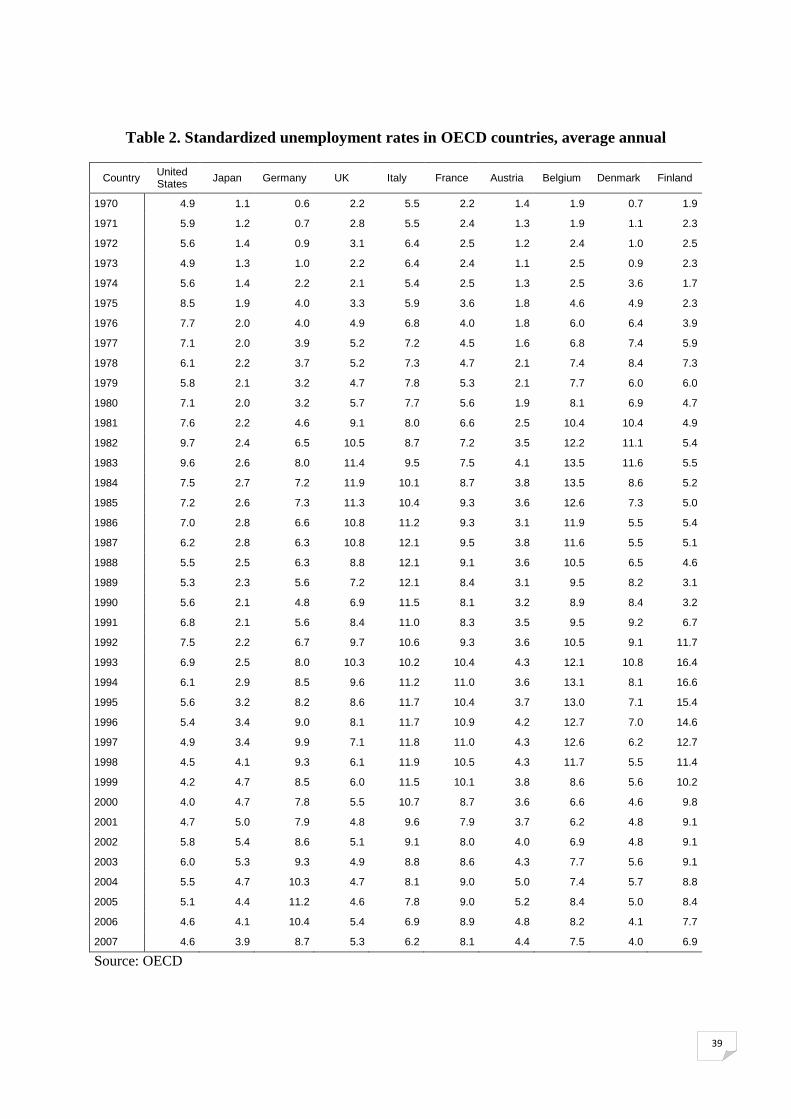
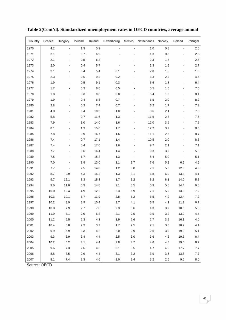
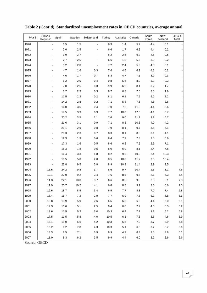
the levels reported in the industrialized countries (see Appendix).
Given the persistently high unemployment rates mentioned above, a search for explanations
by macroeconomists has led to rich theoretical, methodological as well as economic policy
debates (see for example Elmeçkov and MacFarlan (1993) and the Policy Board for
Employment (2007) for a relatively complete synthesis of these arguments). At the center of
these widely shared ideas is the hypothesis of hysteresis which according to the seminal paper
of Blanchard and Summers (1986), reflects a kind of memory of events leading to the
immutability of unemployment even in the presence of changing circumstances in the labour
market. By focusing on the situation in Trinidad and Tobago and Barbados, Downes (1998)
and Craigwell and Warner (1999) respectively are probably the first studies to have
undertaken an investigation on persistence and hysteresis in unemployment in the Caribbean.

4
They demonstrated the existence of ‘persistence’ whereby the unemployment rate affects the
'natural rate of unemployment'. Borda (2000) also showed that this theory is verified in the
case of Guadeloupe. More recently, Ball and Hofstetter (2009) have examined 20 countries in
Latin America and the Caribbean (excluding Barbados and Trinidad and Tobago) and
provided evidence that suggest that hysteresis is reflected in the unemployment situation in
the countries considered. Also, by conducting a theoretical and numerical analysis of a
rational expectations model which include the role of insiders in the labour market, Borda and
Mamingi (2009) have demonstrated that the hysteresis phenomenon must be considered as an
explanation of labour market fluctuations in Barbados, Jamaica and Trinidad and Tobago.
This paper, like previous authors, explores the hypothesis of hysteresis in the English-
speaking Caribbean to see if it is consistent with the observed facts. However, there are two
notable differences between this work and the earlier research. The first concerns the wealth
of the database. The series used for the two English-speaking Caribbean countries – Barbados
and Trinidad and Tobago - are quarterly covering a fairly long period (1975 to 2010 and 1971
to 2010 respectively). The second difference relates to the methodology. The empirical tests
implemented here are based on time series methods recently employed for the econometric
analysis of the labour market, that is, threshold models and processes with nonlinearities in
the mean are utilized.
2. Unemployment in the Caribbean: A Comparison
2.1. The Data
Quarterly unemployment time series data for Barbados and Trinidad and Tobago that spans
nearly five decades are used in the empirical investigations below. For Trinidad and Tobago,
the data set was available over the sample period of 1971Q1 to 2010Q4 and was procured
5
from various issues of the Annual Labour Force Report published by the Central Statistical
Office of Trinidad and Tobago. In the case of Barbados, the data covered the period 1975Q1
to 2010Q4 and was sourced from the Continuous Household Labour Force Survey undertaken
by the Barbados Statistical Service.
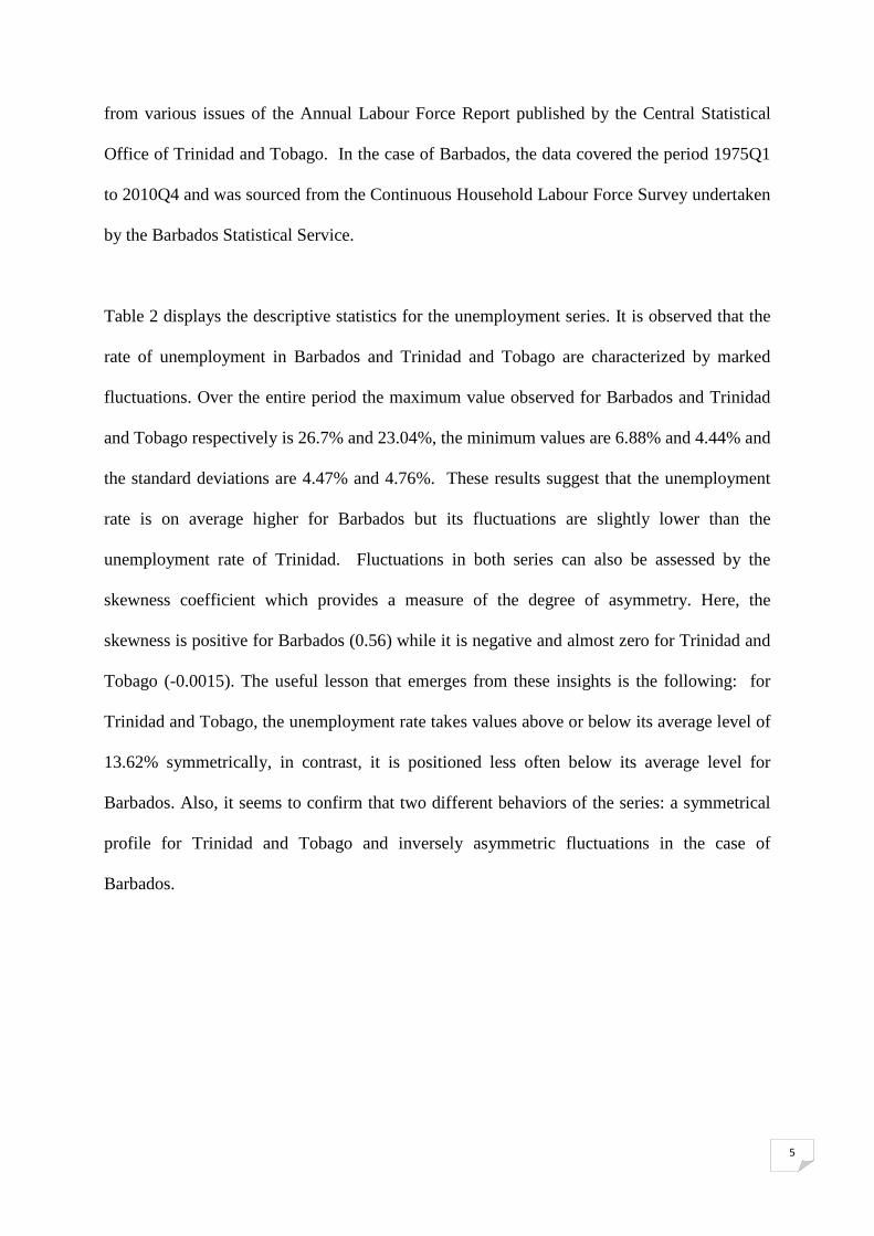
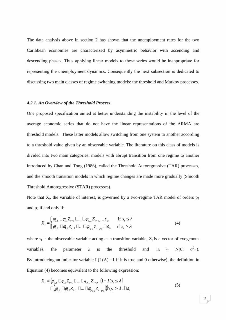
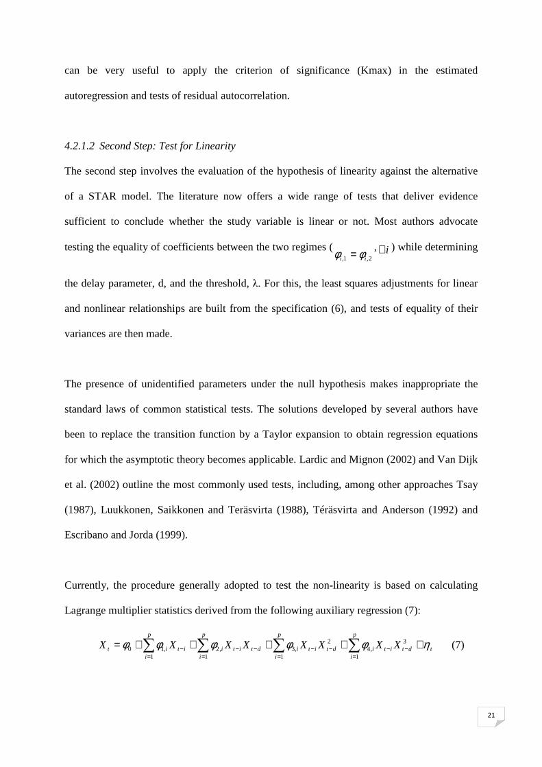
Table 2 displays the descriptive statistics for the unemployment series. It is observed that the
rate of unemployment in Barbados and Trinidad and Tobago are characterized by marked
fluctuations. Over the entire period the maximum value observed for Barbados and Trinidad
and Tobago respectively is 26.7% and 23.04%, the minimum values are 6.88% and 4.44% and
the standard deviations are 4.47% and 4.76%. These results suggest that the unemployment
rate is on average higher for Barbados but its fluctuations are slightly lower than the
unemployment rate of Trinidad. Fluctuations in both series can also be assessed by the
skewness coefficient which provides a measure of the degree of asymmetry. Here, the
skewness is positive for Barbados (0.56) while it is negative and almost zero for Trinidad and
Tobago (-0.0015). The useful lesson that emerges from these insights is the following: for
Trinidad and Tobago, the unemployment rate takes values above or below its average level of
13.62% symmetrically, in contrast, it is positioned less often below its average level for
Barbados. Also, it seems to confirm that two different behaviors of the series: a symmetrical
profile for Trinidad and Tobago and inversely asymmetric fluctuations in the case of
Barbados.

6
Figure 2-A and 2-B. Descriptive Statistics for the Unemployment Rate
0
4
8
12
16
20
6 8 10 12 14 16 18 20 22 24 26
Series: UNEMP_BDOSSample 1975Q4 2010Q3Observations 140
Mean 14.14647Median 14.19257Maximum 26.67155Minimum 6.882642Std. Dev. 4.476381Skewness 0.561394Kurtosis 2.635762
Jarque-Bera 8.127706Probability 0.017183
0
2
4
6
8
10
12
5.0 7.5 10.0 12.5 15.0 17.5 20.0 22.5
Series: UNEMP_TTSample 1970Q1 2010Q2Observations 162
Mean 13.62174Median 13.48457Maximum 23.03663Minimum 4.441273Std. Dev. 4.766949Skewness -0.001467Kurtosis 2.302338
Jarque-Bera 3.285498Probability 0.193448

7
2.2. The Stylized Facts
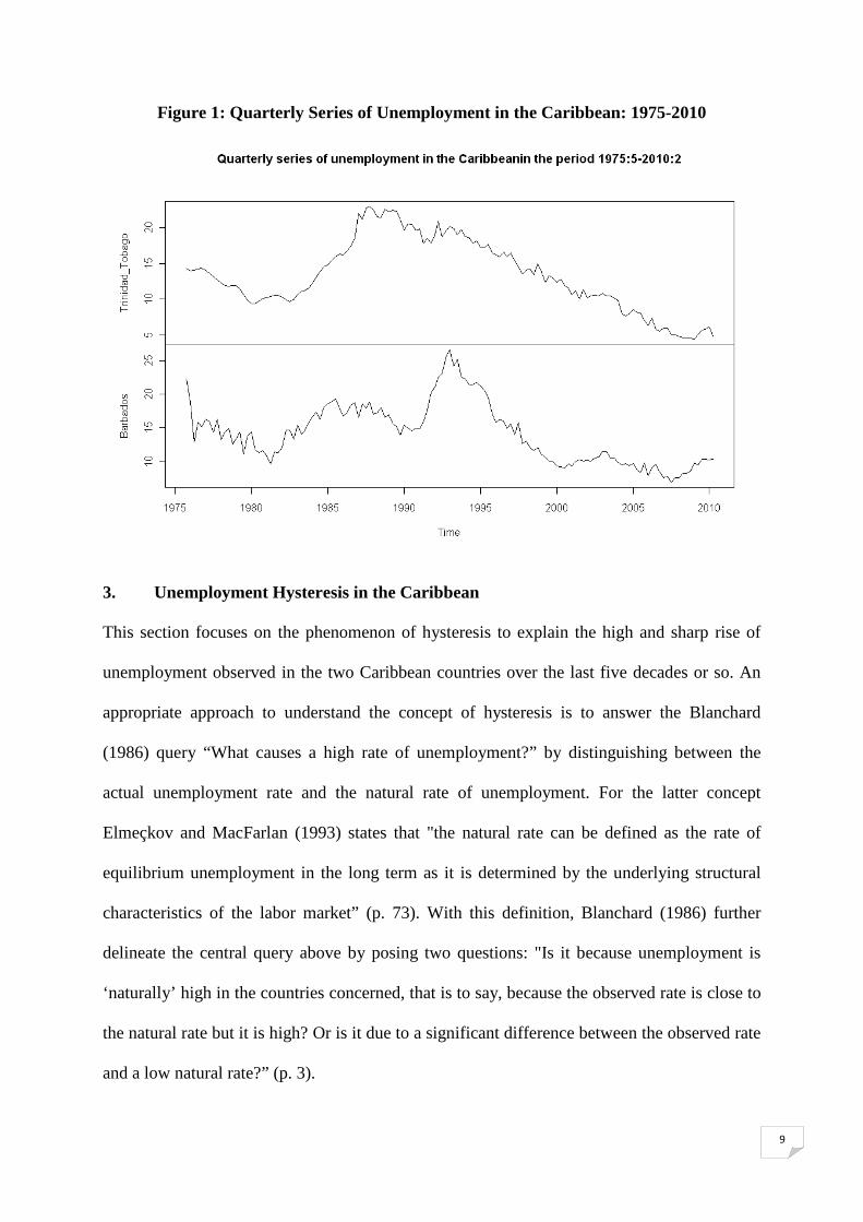
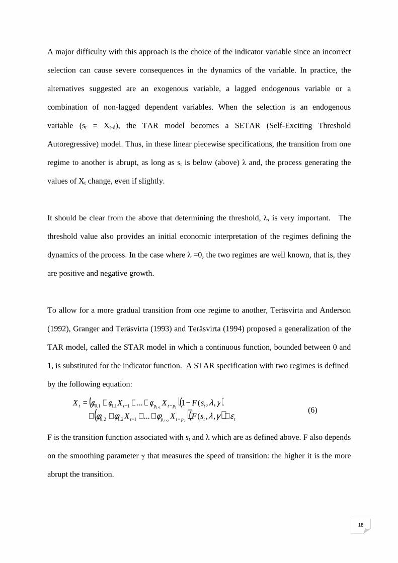
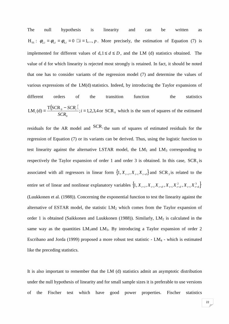
Figure 1 shows that in the case of Trinidad and Tobago the trend in unemployment is
characterised by significant fluctuations, particularly after 1989. Between 1970 and 1972,
unemployment increased by 43.5 percent, but later declined in 1973 and 1975 from 69,800 in
Q1 of 1973 to 51,600 in Q4 of that year, and from 60,800 in Q1 of 1975 to 57,600 in Q4.
Conversely, 1974 and 1976 represented periods of recovery due to the revenue effects of
rising oil prices.
During the period from 1977 to 1983, unemployment followed a general downward trend
despite rebounding slightly from time to time. From 1983 to 1989, the reverse was true, as
unemployment recorded extremely high growth rates. For example, in 1984, 1985 and 1987
the growth rates were 27.6 percent, 16.3 percent and 31.5 percent, respectively. These large
increases continued into 1988, when unemployment reached approximately 100,000. In 1990
and 1991 employment rebounded somewhat, but this improvement was short-lived, as
unemployment began to rise once again in 1991 and 92 when the world economy slipped
further into recession. After the recession unemployment in Trinidad and Tobago continued
on a declining path as that economy benefitted from high oil revenues as a result of increasing
oil prices.
With respect to Barbados, a first glance at Figure 1 reveals that the unemployment rate
appears to be a relatively unstable variable, whose path seems to be a combination of three
curves. The first curve spans the period 1975 to 1981. In 1975, Barbados’ unemployment
rate reached an alarming 22.5 percent. It then declined gradually, following a linear trend,
until 1981, when it registered its third-lowest level for the period.

8
The second curve refers to the years 1982 to 1991, during which unemployment experienced
significant changes, first increasing from 11.4 percent in 1982Q1 to 19.8 percent in 1985Q3,
then fluctuating around a relatively high figure of over 15 percent until 1989Q3, after which it
contracted marginally until 1990Q4.
The third curve, which relates to the period 1991 to 2010, is parabolic in form. The upward-
sloping portion of this parabola represents the years 1991 to 1993, a recessionary period for
the Barbadian economy. This period was characterised by an eight-percentage salary cut for
public workers, massive lay-offs and a rate of unemployment that steadily increased from
17.3 percent in 1990 to 23 percent in 1992, then to 25.1percent in 1992Q4 and 27.1percent in
1993Q1. The downward-sloping portion shows a spectacular decline in the unemployment
rate from nearly 30 percent in 1993 to 9.3 percent by 2000Q1. This drop was due mainly to
the effects of prudent policy actions, a reduction in the labour force resulting from emigration,
and adjustments made after the census found that prior population estimates were too low.
From 2001 to 2003 the unemployment rate rose again as economic growth slowed after the
2001 terrorist attacks in the United States. Afterwards the rate trended down as the economy
picked up. This continued until the start of the current recession in 2008 when there were
some job losses and unemployment expanded again.
9
Figure 1: Quarterly Series of Unemployment in the Caribbean: 1975-2010
3. Unemployment Hysteresis in the Caribbean
This section focuses on the phenomenon of hysteresis to explain the high and sharp rise of
unemployment observed in the two Caribbean countries over the last five decades or so. An
appropriate approach to understand the concept of hysteresis is to answer the Blanchard
(1986) query “What causes a high rate of unemployment?” by distinguishing between the
actual unemployment rate and the natural rate of unemployment. For the latter concept
Elmeçkov and MacFarlan (1993) states that "the natural rate can be defined as the rate of
equilibrium unemployment in the long term as it is determined by the underlying structural
characteristics of the labor market” (p. 73). With this definition, Blanchard (1986) further
delineate the central query above by posing two questions: "Is it because unemployment is
‘naturally’ high in the countries concerned, that is to say, because the observed rate is close to
the natural rate but it is high? Or is it due to a significant difference between the observed rate
and a low natural rate?” (p. 3).
10
The difficulties in answering these questions are related primarily to the fact that the natural
rate of unemployment is not an easy concept to define; it is not a statistically directly
observable and its estimated value may vary from one period to another. Given these two
features of the natural rate, Blanchard (1986) cites the phenomenon of hysteresis as a third
property which makes it hard to estimate ‘the natural rate’ [which] is partially determined by
the rate observed. Therefore, the natural rate of a given period may have determinants from
the previous juncture. In other words, hysteresis reflects the idea that a temporary negative
impact on demand which push up the actual level of unemployment may have a resultant
increase in structural unemployment; it may persist even after the recovery in demand.
In theoretical terms, the explanations that are given for hysteresis are varied. The two
hypotheses that are often echoed by economists are the Insider-Outsider phenomenon and low
employability of long-term unemployed. The idea of "Insider-Outsider”, discussed in
Lindbeck and Snower (1988), blames the situation of hysteresis in unemployment on the
unions. It is argued that workers who are already employed ("insiders") do not take into
account the situation of "outsiders"; their bargaining power is used for the sole purpose of
fixing the nominal wage that would be consistent with maintaining existing jobs and when a
recession occurs because aggregate demand decreases (and, in general, is not anticipated) it
follows that there will be an expansion in the volume of outsiders because of layoffs in
companies. Subsequently, in the good times of the cycle, during recovery, previously
dismissed workers will not be rehired due to renegotiations of contracts requiring insiders’
increases in wages. Thus, the number of excluded workers would tend to grow over the long
term.
11
The explanation for the low employability of long-term unemployed is to assume that when a
person goes through a long period of unemployment, it is likely that its human capital (its
working capacity, technical expertise, productivity) will deteriorate. Such an unemployed
person would have difficulty in re-entering the work place and if lucky, may take a temporary
job. In all cases, the consequence is an increase in unemployment in the long term.
With unemployment rates persistently high between 20 per cent and 30 per cent in some
countries in the Caribbean, the phenomenon of unemployment hysteresis may offer a viable
explanation. On the causes of unemployment in Caribbean countries, Downes (1998)
conducted a very interesting analysis of unemployment in Trinidad and Tobago. He tests a co-
integrated econometric model that allows unemployment to depend on input prices, gross
domestic product, labor market regulations and technical changes. An important conclusion of
his study is the validation of the hypothesis of hysteresis, that is, he found that a one percent
change in the unemployment rate in the previous period can lead to a 0.51 percent change in
the current unemployment rate. Recall that the hysteresis theory suggests that the natural or
equilibrium rate of unemployment depends on the history of the actual unemployment rate.
Craigwell and Warner (1999) determine some of the causes of unemployment in Barbados
over the years 1980 to 1996 by using the Autoregressive Distributed Lag methodology. The
findings indicate that wages paid by the employer is one of the major determinants of the
unemployment rate, and therefore, a reduction in social security taxes may be considered as a
possible remedy for reducing this rate. Other factors affecting unemployment were the high
levels of hiring and firing costs, indicating that labour market legislation should be re-
examined as a policy to combat unemployment. As with Downes (1998) for Trinidad and
Tobago this study validated the hypothesis of hysteresis, that is, the authors found that there is
12
significant persistence in employment, as the sum of the lagged values of employment in the
distributed lag model is relatively high at 0.80.
In addition to these economic explanations of unemployment fluctuations, it is useful for the
purpose of this study to dissect the path of the unemployment series to identify whether it is
linear or nonlinear and stationary or nonstationary. In this context, Figure 1 depicts some
particularly interesting characteristics of these two unemployment data sets : (i) as seen in
most industrialized countries, the unemployment rates in Barbados and Trinidad and Tobago
behave asymmetrically, indicating that faster growth exists during adverse shocks and
smaller decreases results from positive shocks over various sub periods; (ii) unemployment in
the Caribbean are characterized by intervals of variation and average levels that are very
much higher than those of most OECD countries (see Table 2 in the Appendix). Indeed the
unemployment rate in Trinidad and Tobago lies between 4.44 percent and 23 percent over the
period 1970:1-2010:2, with an average rate of 13.6 percent, and for Barbados it is between 9
percent and 26.7 percent over the period 1975:4-2010:3, and the average rate is 14.14 percent.
These rates are well above , up to twice the average in certain periods, those of the G20
countries (South Africa, Germany, Saudi Arabia, Argentina, Australia, Brazil, Canada ,
China, South Korea, United States, France, India, Indonesia, Italy, Japan, Mexico, United
Kingdom, Russia, Turkey, European Union;(iii) the path of unemployment in Trinidad and
Tobago is quite perculiar as it is one of the few nations in the world where there is a period of
a long decline, almost two decades since its record high of 22 percent reported in 1987; (iv)
the trend in the unemployment rate in Barbados is represented by several changes, consisting
of two periods of increases and three episodes of decreases between 1975:4 and 2001:1
followed by a period of smaller fluctuations from 2001: 2 and 2010:3. The configuration of
this trajectory also shows that the upward change in the unemployment rate appear relatively
fast compared to that of its downward movement.

13
4. An Empirical Examination of the Hysteresis Hypothesis
In line with the empirical studies done on various regions in the world, see for example
Phaneuf (1988), Trabelsi (1997), and the Policy Board for Employment (2007), this paper
checks for the presence of hysteresis by implementing different techniques from time series
econometrics. First, unit root tests that highlight the statistical properties of the economic
variables and the interpretation of their non-stationarity in terms of long memory are applied.
Then nonlinear regime switching models that aim at verifying the idea that the dynamics of
the unemployment rate depends on the speed in which it is located are employed. All the
calculations are done with the econometric softwares RATS, EVIEWS and R, the first two for
everything dealing with the unit root analysis and the third for the nonlinear modeling.
4.1 Unit Roots Tests
The graphic examination of the unemployment rates above in section 2 shows some level of
instability. In the case of Barbados, it is clear that the evolution is not stable over time, as the
unemployment series varies around different average values. For Trinidad and Tobago, this
instability is a reflection of long periods of growth or decay and the existence of average
levels that change from one sub-period to another. Given the recent results in the literature on
economic time series, it is accepted that this instability may have two major origins. On the
one hand, it may be the result of non-stationarity. On the other hand, it may be due to non-
linear behaviours such as switching from one unemployment regime to another.
In the tradition of empirical studies that test for hysteresis in unemployment, the following
commonly used unit root tests - Dickey-Fuller, Phillips-Perron and Kwiatkowski, Phillips,
Schmidt and Shin (KPSS) - are implemented. The results of these procedures are reported in
Table 1 and they validate the hypothesis of a unit root, implying that the hypothesis of
hysteresis for the two countries selected is upheld. However, in the event that the data-
14
generating process of the unemployment rate is actually a non-linear but stationary process, it
is well recognized that these traditional tests exhibit low power and can lead one to wrongly
accept the hypothesis of non-stationarity. It is then necessary to examine the order of
integration taking into account possible nonlinear effects. In this regard the extension of the
Dickey-Fuller test proposed by Kapetanios et al. (2003) (KSS) is considered. This procedure
provides a statistical framework to test the alternative "non-stationarity and stationarity and
linearity versus nonlinearity" hypothesis.
The starting point for the KSS method is similar to the DF regression test and incorporates the
nonlinearity by means of an autoregressive specification for thresholds with exponential
transition function:
( )[ ] tttt XXX εθγ +−−=∆ −−2
11 exp1 (1)
where the series tX is in deviation form from its trend, and the parameter tε ~ );0( 2εσN and
0≥θ is used to modulate the speed of transition. The null hypothesis H0: 0=θ must be
tested against the alternative hypothesis H1: 0>θ . However, since the parameter γ is not
identified under H0, Kapetanios et al. (2003) have proposed a re-parameterization based on
Taylor series approximation. This gives a regression equation that allows the test to be easily
implemented:
ttt XX εδ +=∆ −3
1 (2)
By introducing the lagged terms of tX to correct for autocorrelation in the errors, a regression
equation analogous to the ADF test is obtained:
t
p
kktktt XXX εγδ ∑
=−− +∆+=∆
1
31 (3)
The DF, ADF and KSS tests share the same null hypothesis of non-stationarity H0: δ = 0
15
while the alternative hypothesis of the Dickey and Fuller stationarity linear KSS test is that of
the stationary nonlinear (H1: δ <0).
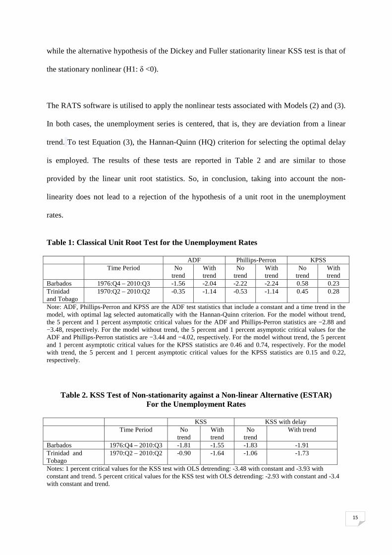
The RATS software is utilised to apply the nonlinear tests associated with Models (2) and (3).
In both cases, the unemployment series is centered, that is, they are deviation from a linear
trend. To test Equation (3), the Hannan-Quinn (HQ) criterion for selecting the optimal delay
is employed. The results of these tests are reported in Table 2 and are similar to those
provided by the linear unit root statistics. So, in conclusion, taking into account the non-
linearity does not lead to a rejection of the hypothesis of a unit root in the unemployment
rates.
Table 1: Classical Unit Root Test for the Unemployment Rates ADF Phillips-Perron KPSS Time Period No
trend With trend
No trend
With trend
No trend
With trend
Barbados 1976:Q4 – 2010:Q3 -1.56 -2.04 -2.22 -2.24 0.58 0.23 Trinidad and Tobago
1970:Q2 – 2010:Q2 -0.35 -1.14 -0.53 -1.14 0.45 0.28
Note: ADF, Phillips-Perron and KPSS are the ADF test statistics that include a constant and a time trend in the model, with optimal lag selected automatically with the Hannan-Quinn criterion. For the model without trend, the 5 percent and 1 percent asymptotic critical values for the ADF and Phillips-Perron statistics are −2.88 and −3.48, respectively. For the model without trend, the 5 percent and 1 percent asymptotic critical values for the ADF and Phillips-Perron statistics are −3.44 and −4.02, respectively. For the model without trend, the 5 percent and 1 percent asymptotic critical values for the KPSS statistics are 0.46 and 0.74, respectively. For the model with trend, the 5 percent and 1 percent asymptotic critical values for the KPSS statistics are 0.15 and 0.22, respectively.
Table 2. KSS Test of Non-stationarity against a Non-linear Alternative (ESTAR) For the Unemployment Rates
KSS KSS with delay Time Period No
trend With trend
No trend
With trend
Barbados 1976:Q4 – 2010:Q3 -1.81 -1.55 -1.83 -1.91 Trinidad and Tobago
1970:Q2 – 2010:Q2 -0.90 -1.64 -1.06 -1.73
Notes: 1 percent critical values for the KSS test with OLS detrending: -3.48 with constant and -3.93 with constant and trend. 5 percent critical values for the KSS test with OLS detrending: -2.93 with constant and -3.4 with constant and trend.
16
4.2 An Analysis of the Family of Regime Switching Models
In recent years, the literature on the prolonged persistence of unemployment has applied
regime switching models to represent the properties of non-linearity in the unemployment rate
and also to provide economic explanations for this behavior. Authors like Trabelsi (1995),
Franses (2004) and Uctum (2007) have emphasized the need for econometric analysis to
capture economic activity that allows for the phenomenon of asymmetry where an economy
goes through different phases of the business cycle involving growth and decline.
In his doctoral thesis, Fouquau (2008, p..) recalls the work of Neftci (1984) and Rothman
(1991) and argued that "bad times to employment are less persistent than the good times,
indicating that falls are certainly more pronounced but of shorter duration.” This observation
is in line with Keynes (...)'s comments on economic fluctuations in the periods of war and
boom, when he noted that the unemployment rate is characterized by abrupt jumps and weak
declines.
Utilizing OECD data, several authors (Refs) have conducted empirical studies to test the
persistence of unemployment and explained it through modeling of volatility shocks from
various sources (such as domestic productivity or domestic monetary policy shocks, as well as
external shocks operating, for example, through the foreign interest rate). Research on
countries outside the developed world is very scarce. However, Moolman (2003) considered
the case of the unemployment rate of South Africa. He used quarterly data for the period 1978
to 2000 to show that total employment and sectoral employment flows are related to the
business cycle. In this context, he applied an autoregressive equation incorporating two
variables as explanatory factors representative of the state of the economy, using a Markov
model with regime changes. Moolman also highlighted that knowledge of the asymmetric
behavior of unemployment is of importance for short-term economic stabilization policies.
17
The data analysis above in section 2 has shown that the unemployment rates for the two
Caribbean economies are characterized by asymmetric behavior with ascending and
descending phases. Thus applying linear models to these series would be inappropriate for
representing the unemployment dynamics. Consequently the next subsection is dedicated to
discussing two main classes of regime switching models: the threshold and Markov processes.
4.2.1. An Overview of the Threshold Process
One proposed specification aimed at better understanding the instability in the level of the
average economic series that do not have the linear representations of the ARMA are
threshold models. These latter models allow switching from one system to another according
to a threshold value given by an observable variable. The literature on this class of models is
divided into two main categories: models with abrupt transition from one regime to another
introduced by Chan and Tong (1986), called the Threshold Autoregressive (TAR) processes,
and the smooth transition models in which regime changes are made more gradually (Smooth
Threshold Autoregressive (STAR) processes).
Note that Xt, the variable of interest, is governed by a two-regime TAR model of orders p1
and p2 if and only if:
>++++
≤++++=
−−
−−
λεφφφλεφφφ
ttptpt
ttptpt
t sZZ
sZZX
if ...
if ...
2,12,12,0
1,11,11,0
222
111 (4)
where st is the observable variable acting as a transition variable, Zt is a vector of exogenous
variables, the parameter λ is the threshold and ɛt ~ N(0; σ2ɛ).
By introducing an indicator variable I (I (A) =1 if it is true and 0 otherwise), the definition in
Equation (4) becomes equivalent to the following expression:
( )( )( )( ) ttptpt
tptptt
sIZZ
sIZZX
ελφφφλφφφ
+>++++
≤−+++=
−−
−−
(...
(1...
222
111
,12,12,0
,11,11,0 (5)
18
A major difficulty with this approach is the choice of the indicator variable since an incorrect
selection can cause severe consequences in the dynamics of the variable. In practice, the
alternatives suggested are an exogenous variable, a lagged endogenous variable or a
combination of non-lagged dependent variables. When the selection is an endogenous
variable (st = Xt-d), the TAR model becomes a SETAR (Self-Exciting Threshold
Autoregressive) model. Thus, in these linear piecewise specifications, the transition from one
regime to another is abrupt, as long as st is below (above) λ and, the process generating the
values of Xt change, even if slightly.
It should be clear from the above that determining the threshold, λ, is very important. The
threshold value also provides an initial economic interpretation of the regimes defining the
dynamics of the process. In the case where λ =0, the two regimes are well known, that is, they
are positive and negative growth.
To allow for a more gradual transition from one regime to another, Teräsvirta and Anderson
(1992), Granger and Teräsvirta (1993) and Teräsvirta (1994) proposed a generalization of the
TAR model, called the STAR model in which a continuous function, bounded between 0 and
1, is substituted for the indicator function. A STAR specification with two regimes is defined
by the following equation:
( )( )( )( ) ttptpt
tptptt
sFXX
sFXXX
εγλφφφγλφφφ
+++++
−+++=
−−
−−
,,(...
,,(1...
222
111
,12,12,0
,11,11,0 (6)
F is the transition function associated with st and λ which are as defined above. F also depends
on the smoothing parameter γ that measures the speed of transition: the higher it is the more
abrupt the transition.
19
In reviewing the STAR literature, Uctum (2007) mentioned two distinct specifications, the
exponential STAR (ESTAR) and the logistic STAR (LSTAR), so called because the
transition functions are based on the logistics function ( ( ) 1)(1),,(−−−+= λγγλ ts
t esF , 0>γ )
and the exponential function (( ( )2)(1),,( λγγλ −−−= tst esF , 0>γ ), respectively. These two
specifications have different dynamics of the mean reversion process. The logistic function
implies an asymmetric adjustment of the series, Xt; accordingly the values are associated
with positive or negative deviations of st from the threshold λ. It is therefore sensitive to the
signs of the deviations (sign effect). Conversely, the exponential function imposes a
symmetric adjustment regardless of the sign of (st - λ); it is sensitive to the magnitude of the
deviations (size effect) rather than the sign. In other words, when the STAR process is
specified based on a logistic function, it is assumed that the positive and negative deviations
of Xt return to their average levels with different speeds. On the contrary, in the case of the
exponential function, the return is made with the same speed as the deviations are positive or
negative.
Uctum (2007) also touched on the economic interpretation of the transition variable. In
particular, he cites Granger and Teräsvirta (1997, p..) as stating that "change at the aggregate
level will be more adequately represented by a STAR model if the economy consists of a
large number of persons or companies each of which switches regime abruptly but at different
times. This non-simultaneity of individual behavior can indeed be justified by the fact that
some individuals or institutional agents can benefit in anticipating government action and
begin the transition before the change of economic policy, while information costs or
adjustment may lead other officers to respond with delay to the action of the authorities. "
Another interpretation is suggested by Maddala (1991, p…) who lament that "the smoothness
20
of the transition may result from the fact that not believing in the permanence of the new
economic policy, economic agents do not adjust immediately to the new regime but converge
gradually through learning."
With elements of the structure and characteristics of threshold models discussed, it remains to
mention the steps of estimating their parameters. In the case of threshold models of the TAR
family, these pitfalls are particularly important because of problems identifying the threshold
variable. As Salem and Perraudin (2001) argued, the choice of the transition variable (or the
delay parameter), and the threshold in a TAR model is not covered by conventional nonlinear
methods, because the likelihood function is not differentiable with respect to these
parameters. For the SETAR specification, identification and estimation of the parameters are
usually conducted on the basis of a scanning procedure over the entire grid of possible values
of λ and d by comparing the log-likelihood function and the information criteria defined for
all possible combinations of d and λ. Once their values are estimated, fixed parameters of the
two regimes can be obtained by applying Ordinary Lease Squares (OLS) to the observations
belonging to each regime. Regarding STAR models, many methods have been proposed in
the literature to achieve phases of identification, estimation and statistical validation. Today, it
seems to be a consensus around a three-step procedure as described by Téräsvirta and
Anderson (1992), Teräsvirta (1994, 1998) and Van Dijk, Teräsvirta and Franses (2000).
4.2.1.1 First step: Identification
This step is dedicated to selecting the optimal value of the delay parameter d which is based
on the review of the information criteria (Teräsvirta (1994)). In addition, since the over and
under-parameterization create significant problems (autocorrelation of errors in the case of
under-parameterization and loss of model performance in the case of over-parameterization) it
21
can be very useful to apply the criterion of significance (Kmax) in the estimated
autoregression and tests of residual autocorrelation.
4.2.1.2 Second Step: Test for Linearity
The second step involves the evaluation of the hypothesis of linearity against the alternative
of a STAR model. The literature now offers a wide range of tests that deliver evidence
sufficient to conclude whether the study variable is linear or not. Most authors advocate
testing the equality of coefficients between the two regimes (2,1, ii φφ =, i∀ ) while determining
the delay parameter, d, and the threshold, λ. For this, the least squares adjustments for linear
and nonlinear relationships are built from the specification (6), and tests of equality of their
variances are then made.
The presence of unidentified parameters under the null hypothesis makes inappropriate the
standard laws of common statistical tests. The solutions developed by several authors have
been to replace the transition function by a Taylor expansion to obtain regression equations
for which the asymptotic theory becomes applicable. Lardic and Mignon (2002) and Van Dijk
et al. (2002) outline the most commonly used tests, including, among other approaches Tsay
(1987), Luukkonen, Saikkonen and Teräsvirta (1988), Téräsvirta and Anderson (1992) and
Escribano and Jorda (1999).
Currently, the procedure generally adopted to test the non-linearity is based on calculating
Lagrange multiplier statistics derived from the following auxiliary regression (7):
t
p
idtiti
p
idtiti
p
idtiti
p
iitit XXXXXXXX ηφφφφφ +++++= ∑∑∑∑
=−−
=−−
=−−
=−
1
3,4
1
2,3
1,2
1,10 (7)
22
The null hypothesis is linearity and can be written as
piiii ,...,1 0 :H ,4,3,201 =∀=== φφφ . More precisely, the estimation of Equation (7) is
implemented for different values of d, Dd ≤≤1 , and the LM (d) statistics obtained. The
value of d for which linearity is rejected most strongly is retained. In fact, it should be noted
that one has to consider variants of the regression model (7) and determine the values of
various expressions of the LM(d) statistics. Indeed, by introducing the Taylor expansions of
different orders of the transition function the statistics
( )4,3,2,1;
SCRT(d)LM
0
0i =
−= i
SCR
SCRi or 0SCR which is the sum of squares of the estimated
residuals for the AR model and iSCR the sum of squares of estimated residuals for the
regression of Equation (7) or its variants can be derived. Thus, using the logistic function to
test linearity against the alternative LSTAR model, the LM1 and LM3 corresponding to
respectively the Taylor expansion of order 1 and order 3 is obtained. In this case, 1SCR is
associated with all regressors in linear form { }dtitit XXX −−− ,1, and 3SCR is related to the
entire set of linear and nonlinear explanatory variables { }32 ,,,1, dtitdtitdtitit XXXXXXX −−−−−−−
(Luukkonen et al. (1988)). Concerning the exponential function to test the linearity against the
alternative of ESTAR model, the statistic LM2 which comes from the Taylor expansion of
order 1 is obtained (Saikkonen and Luukkonen (1988)). Similarly, LM2 is calculated in the
same way as the quantities LM1and LM3. By introducing a Taylor expansion of order 2
Escribano and Jorda (1999) proposed a more robust test statistic - LM4 - which is estimated
like the preceding statistics.
It is also important to remember that the LM (d) statistics admit an asymptotic distribution
under the null hypothesis of linearity and for small sample sizes it is preferable to use versions
of the Fischer test which have good power properties. Fischer statistics
23
( )4,3,2,1;
/
/SCR(d)LM
20
110i =
−= i
vSCR
vSCR are calculated with v1 and v2 as the appropriate
numbers of degrees of freedom.
The final step in testing for linearity comes after the rejection of linearity. It is dedicated to
the choice between the ESTAR and LSTAR models and is conducted on the basis of a series
of nested hypotheses:
pii ,...,1 0 :H ,404 ==φ
piii ,...,1 0/0 :H ,4,303 === φφ
piiii ,...,1 0/0 :H ,4,3,202 ==== φφφ .
The decision rule is as follows:
- The rejection of 0 :H ,404 =iφ allows one to accept the selection of LSTAR specification.
- When 04H is accepted, proceed to test the hypothesis 0;0 :H ,4,303 == ii φφ . If rejected the
conclusion is the validation of the ESTAR specification.
- If 0;0 :H ,4,303 == ii φφ is accepted, go and test 0;0 :H ,4,3,202 === iii φφφ . The rejection of
this hypothesis allows one then to conclude in favor of a LSTAR specification.
As an alternative approach to decide on the appropriate form of the transition function,
Escribano and Jorda (1999) have opted for a solution based on the application of two separate
tests instead of a single hypothesis test. For this, they evaluate the
assumptions piiiE ,...,1 0 :H ,4,20 === φφ and piiiL ,...,1 0 :H ,3,10 === φφ and accept the
LSTAR model (ESTAR) if the highest value of the Fischer statistic is obtained for E0H
( L0H ).
24
4.2.1.3 Step Three: Estimation
In contrast to the previous step of identification, a more systematic approach can be used to
estimate the selected model. Of course, once the transition function and the transition variable
have been determined, nonlinear least squares estimators can be computed by applying an
iterative numerical optimization algorithm. Several estimation strategies can be employed (see
Teräsvirta (1994), van Dijk, Terasvirta and Franses (2002) and Uctum (2007)).
However, it is difficult to validate their content. Indeed, in practice the complexity of
estimating parameters of the STAR model are linked to the inherent difficulty of properly
selecting the threshold variable (see Uctum (2007, p. 454). For example, regarding the
estimation of the transition parameters γ and λ, Tsay (2005, p. 163) notes that "experience
shows that the transition parameters γ and λ of a STAR model are hard to estimate. In
particular, most empirical studies show that standard errors of the estimates of γ and λ are
often quite large, resulting in t-ratios of about 1.0 ".
It is also important to add that the nature of the data that these models depend on has an
impact on the quality of the results of the econometric adjustment operations. For instance,
whether good or bad results of estimating specification (6) are obtained depend on if the series
of interest is in levels, differences or deviation from trend. The empirical literature on the
unemployment rate suggests that all of these prior transformations are used from time to time.
For example, Rothman (1998) considered several nonlinear models on level data, deviation
from a linear trend and filtered by applying the Hildeth and Prescod method. Skalin and
Teräsvirta (2002) conducted their modeling effort directly on the raw quarterly data of 11
OECD countries, not seasonally adjusted. Similarly, Akram (2005) has identified these types
of data adjustments when estimating LSTAR models. In more recent articles such as that of
Franchi and Ordóñez (2009), the authors apply LSTAR models for Spain directly on raw data

25
prior to retaining the assumption of stationarity of the unemployment rate around multiple
structural changes.
4.2.2. Empirical Results
To implement the nonlinear time series models within the R platform, tsDyn, TSA and
BayStar packages are the most utilized in the literature (see Antonio et al. (2008)). In this
paper, the tsDyn package developed by Antonio et al. (2008) and the less known but very
powerful RSTAR library propounded by Balcılar Mehmet (2009) are used.
4.2.2.1 Identification
In the tradition of modeling linear stochastic processes AR models that best represent the
unemployment rate series (in first differences) are selected and estimated using the software
Eviews. The model selection criteria employed are the Akaike and Baysian methods along
with several statistical validation tests, especially those related to the behavior of non-
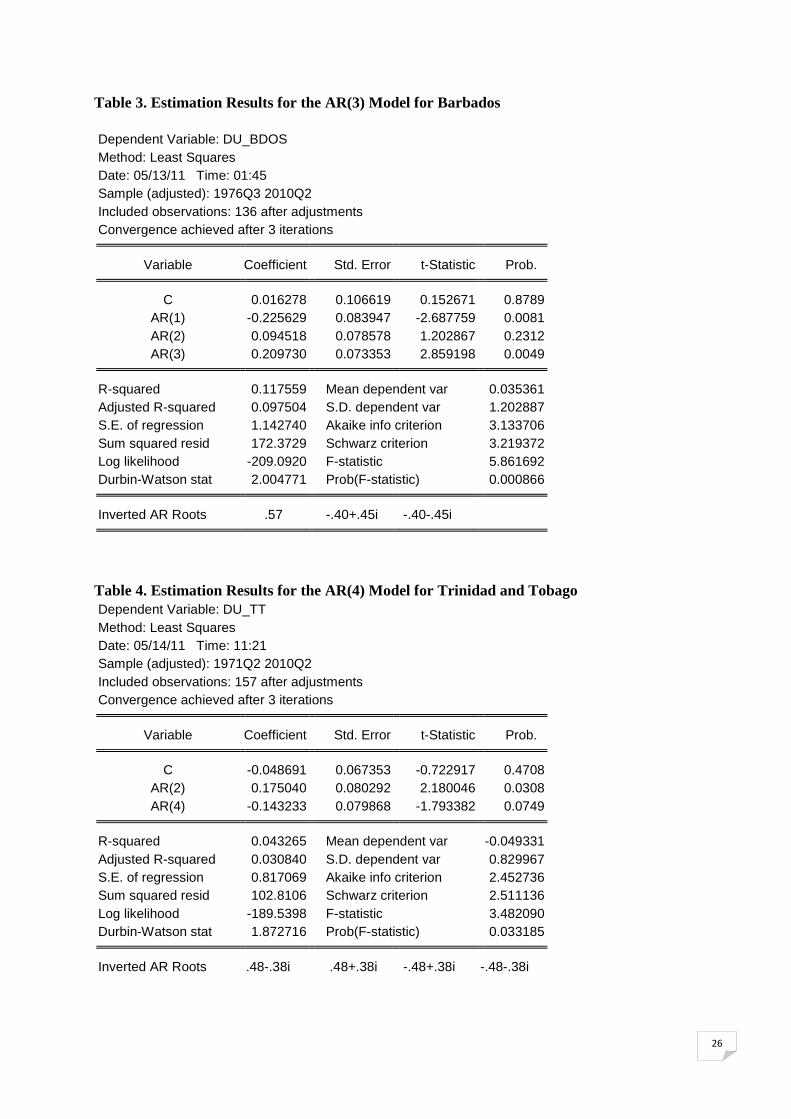
autocorrelation, homoscedasticity and Gaussian noise. The AR models that gave the best
performances are respectively AR (3) for Barbados and AR (4) for Trinidad and Tobago (see
Table 3 and table 4).
4.2.2.1 Tests of Linearity
The unit root tests have provided information on the non-stationarity of the unemployment
rates but not on their linearity. These series should therefore be placed in the general LM
testing framework explained above. To this end, the package RSTAR (Balcilar Mehmet
(2009)) which has the advantage of being able to implement many of the tests proposed by
Van Dijk, Teräsvirta and Franses (2002) is used. Thus, LM1, LM2, LM3, and LM3e and LM4
calculated by RSTAR correspond in sequence to the statistics LM1, LM2, LM3, LM3e
26
Table 3. Estimation Results for the AR(3) Model for Barbados
Dependent Variable: DU_BDOS Method: Least Squares Date: 05/13/11 Time: 01:45 Sample (adjusted): 1976Q3 2010Q2 Included observations: 136 after adjustments Convergence achieved after 3 iterations
Variable Coefficient Std. Error t-Statistic Prob. C 0.016278 0.106619 0.152671 0.8789
AR(1) -0.225629 0.083947 -2.687759 0.0081 AR(2) 0.094518 0.078578 1.202867 0.2312 AR(3) 0.209730 0.073353 2.859198 0.0049
R-squared 0.117559 Mean dependent var 0.035361
Adjusted R-squared 0.097504 S.D. dependent var 1.202887 S.E. of regression 1.142740 Akaike info criterion 3.133706 Sum squared resid 172.3729 Schwarz criterion 3.219372 Log likelihood -209.0920 F-statistic 5.861692 Durbin-Watson stat 2.004771 Prob(F-statistic) 0.000866
Inverted AR Roots .57 -.40+.45i -.40-.45i
Table 4. Estimation Results for the AR(4) Model for Trinidad and Tobago Dependent Variable: DU_TT Method: Least Squares Date: 05/14/11 Time: 11:21 Sample (adjusted): 1971Q2 2010Q2 Included observations: 157 after adjustments Convergence achieved after 3 iterations
Variable Coefficient Std. Error t-Statistic Prob. C -0.048691 0.067353 -0.722917 0.4708
AR(2) 0.175040 0.080292 2.180046 0.0308 AR(4) -0.143233 0.079868 -1.793382 0.0749
R-squared 0.043265 Mean dependent var -0.049331
Adjusted R-squared 0.030840 S.D. dependent var 0.829967 S.E. of regression 0.817069 Akaike info criterion 2.452736 Sum squared resid 102.8106 Schwarz criterion 2.511136 Log likelihood -189.5398 F-statistic 3.482090 Durbin-Watson stat 1.872716 Prob(F-statistic) 0.033185
Inverted AR Roots .48-.38i .48+.38i -.48+.38i -.48-.38i
27
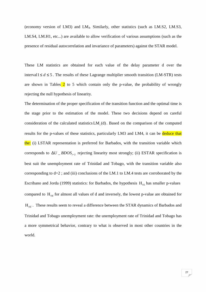
(economy version of LM3) and LM4. Similarly, other statistics (such as LM.S2, LM.S3,
LM.S4, LM.H1, etc...) are available to allow verification of various assumptions (such as the
presence of residual autocorrelation and invariance of parameters) against the STAR model.
These LM statistics are obtained for each value of the delay parameter d over the
interval 51 ≤≤ d . The results of these Lagrange multiplier smooth transition (LM-STR) tests
are shown in Tables 2 to 5 which contain only the p-value, the probability of wrongly
rejecting the null hypothesis of linearity.
The determination of the proper specification of the transition function and the optimal time is
the stage prior to the estimation of the model. These two decisions depend on careful
consideration of the calculated statistics (d)LM i . Based on the comparison of the computed
results for the p-values of these statistics, particularly LM3 and LM4, it can be deduce that
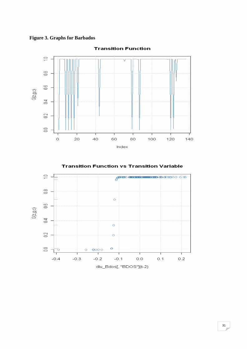
the: (i) LSTAR representation is preferred for Barbados, with the transition variable which
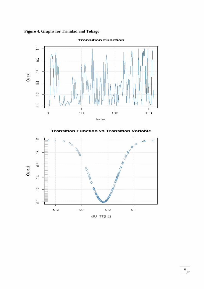
corresponds to 2_ −∆ tBDOSU rejecting linearity most strongly; (ii) ESTAR specification is
best suit the unemployment rate of Trinidad and Tobago, with the transition variable also
corresponding to d=2 ; and (iii) conclusions of the LM.1 to LM.4 tests are corroborated by the
Escribano and Jorda (1999) statistics: for Barbados, the hypothesis L0H has smaller p-values
compared to E0H for almost all values of d and inversely, the lowest p-value are obtained for
E0H . These results seem to reveal a difference between the STAR dynamics of Barbados and
Trinidad and Tobago unemployment rate: the unemployment rate of Trinidad and Tobago has
a more symmetrical behavior, contrary to what is observed in most other countries in the
world.
28
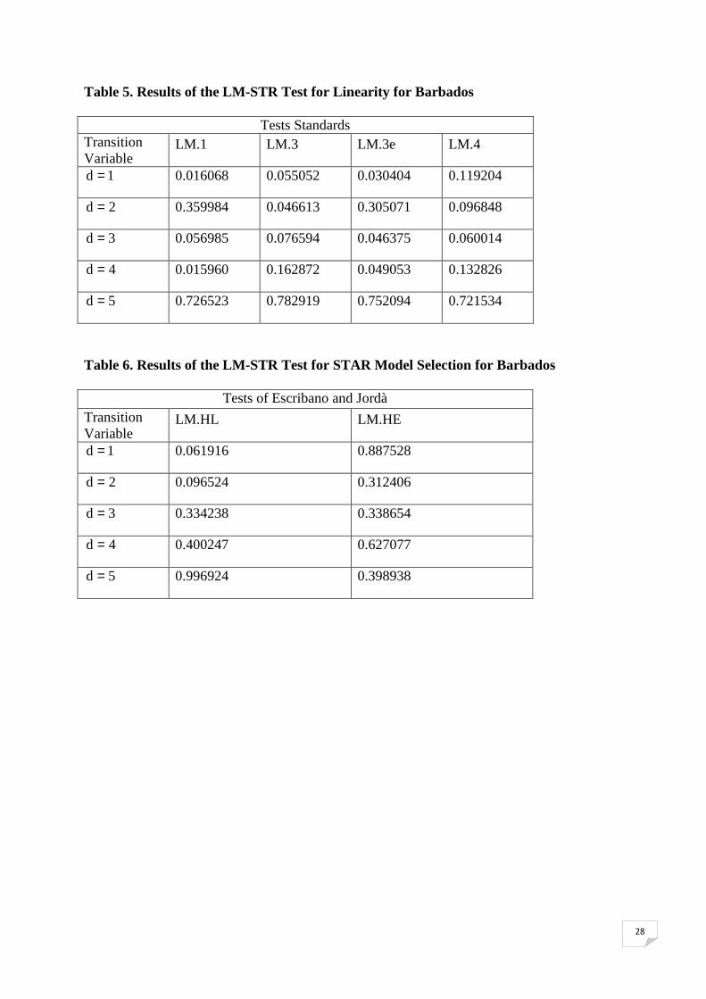
Table 5. Results of the LM-STR Test for Linearity for Barbados
Tests Standards Transition Variable
LM.1 LM.3 LM.3e LM.4
1d = 0.016068 0.055052 0.030404 0.119204
2d = 0.359984 0.046613 0.305071 0.096848
3d = 0.056985 0.076594 0.046375 0.060014
4d = 0.015960 0.162872 0.049053 0.132826
5d = 0.726523 0.782919 0.752094 0.721534
Table 6. Results of the LM-STR Test for STAR Model Selection for Barbados
Tests of Escribano and Jordà Transition Variable
LM.HL LM.HE
1d = 0.061916 0.887528
2d = 0.096524 0.312406
3d = 0.334238 0.338654
4d = 0.400247 0.627077
5d = 0.996924 0.398938
29
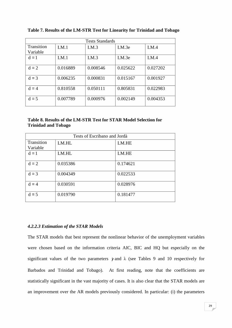
Table 7. Results of the LM-STR Test for Linearity for Trinidad and Tobago
Tests Standards Transition Variable
LM.1 LM.3 LM.3e LM.4
1d = LM.1 LM.3 LM.3e LM.4
2d = 0.016889 0.008546 0.025622 0.027202
3d = 0.006235 0.000831 0.015167 0.001927
4d = 0.810558 0.050111 0.805831 0.022983
5d = 0.007789 0.000976 0.002149 0.004353
Table 8. Results of the LM-STR Test for STAR Model Selection for Trinidad and Tobago
Tests of Escribano and Jordà Transition Variable
LM.HL LM.HE
1d = LM.HL LM.HE
2d = 0.035386 0.174621
3d = 0.004349 0.022533
4d = 0.030591 0.028976
5d = 0.019790 0.181477
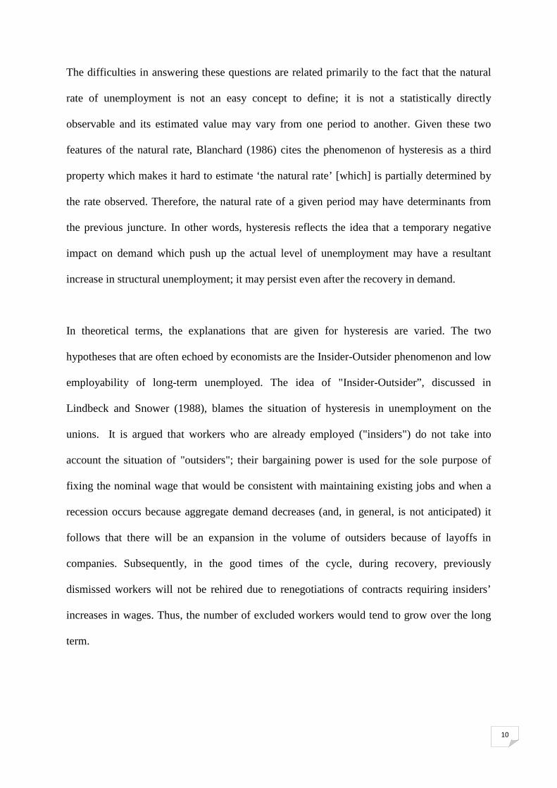
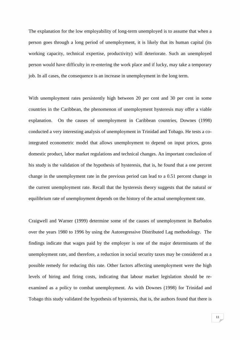
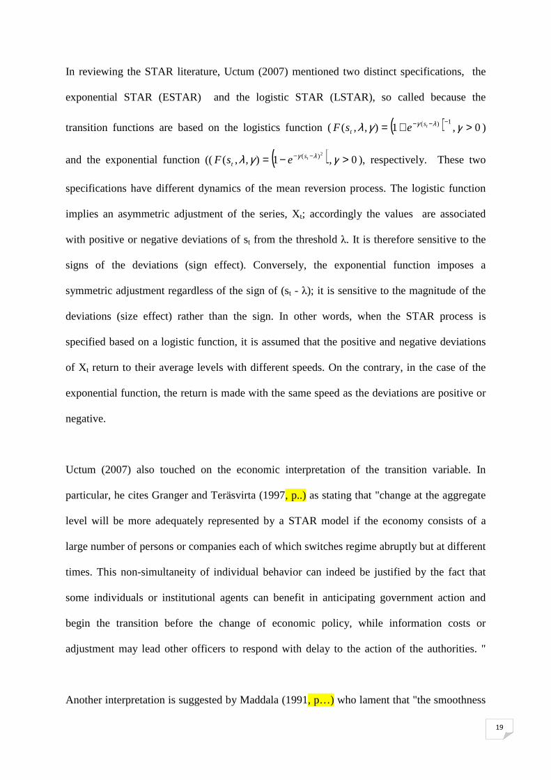
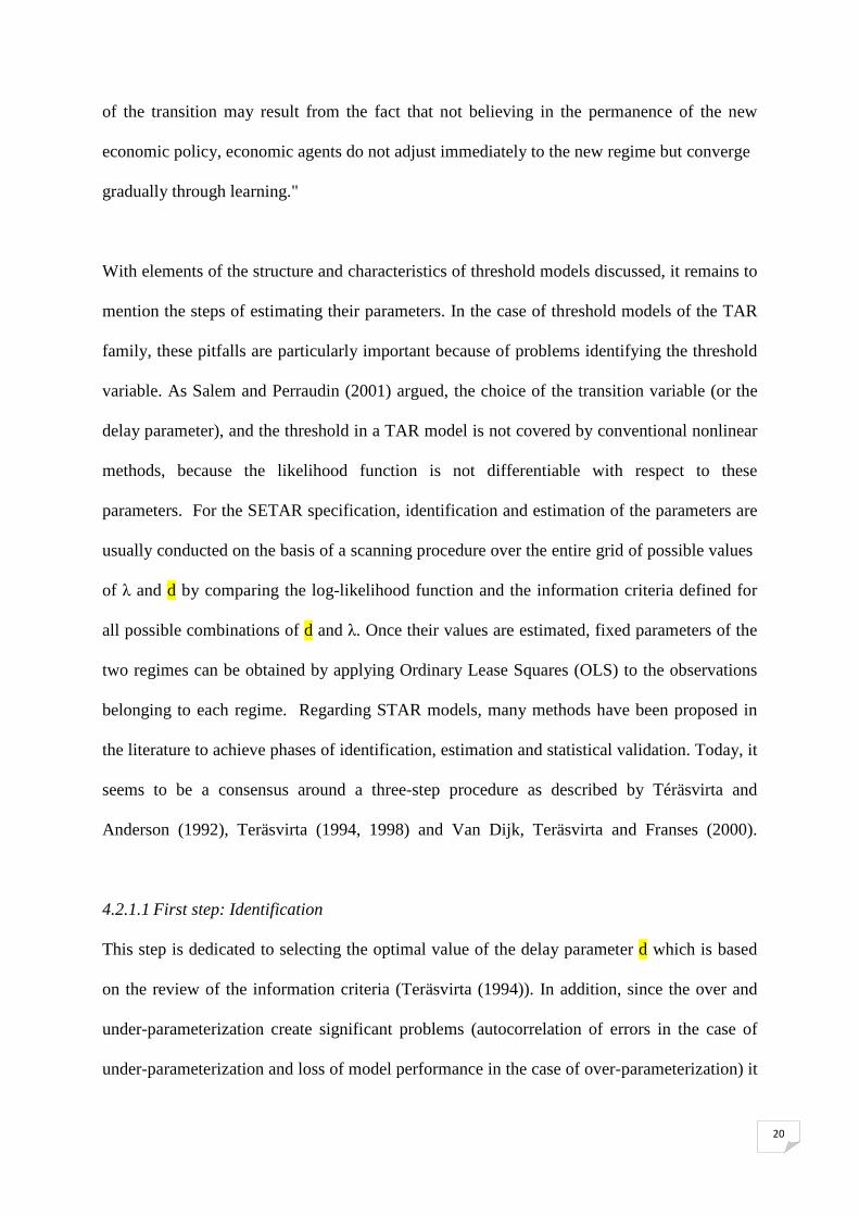
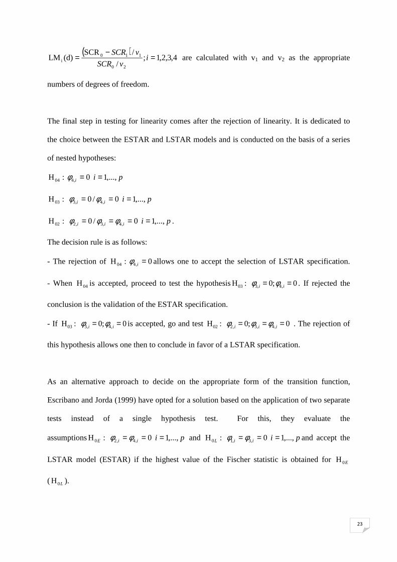
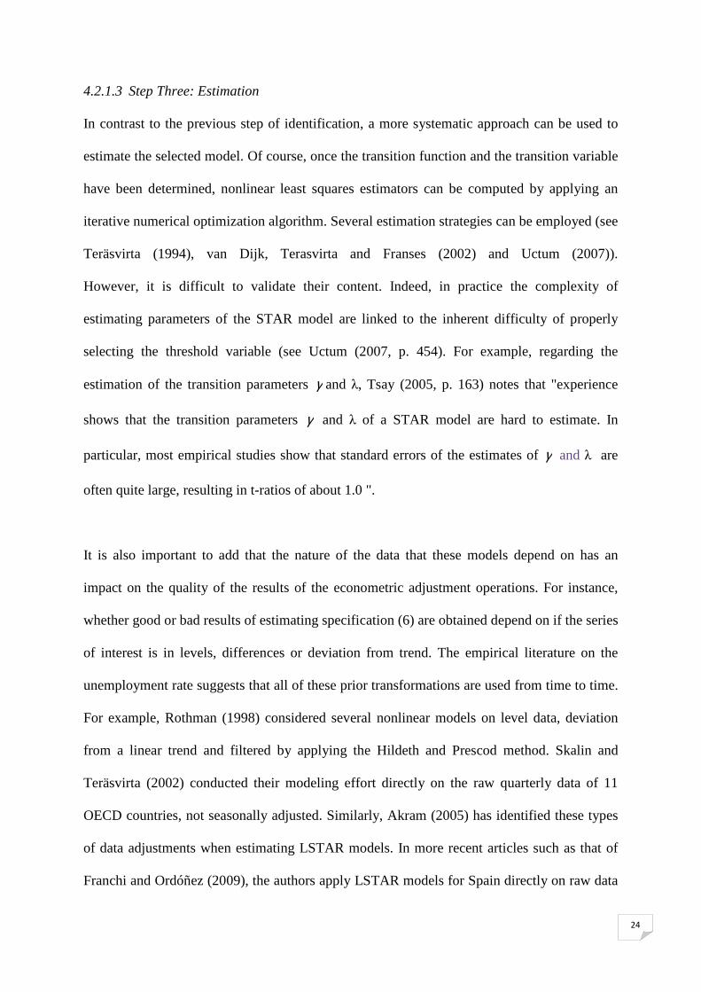
4.2.2.3 Estimation of the STAR Models
The STAR models that best represent the nonlinear behavior of the unemployment variables
were chosen based on the information criteria AIC, BIC and HQ but especially on the
significant values of the two parameters γ and λ (see Tables 9 and 10 respectively for
Barbados and Trinidad and Tobago). At first reading, note that the coefficients are
statistically significant in the vast majority of cases. It is also clear that the STAR models are
an improvement over the AR models previously considered. In particular: (i) the parameters
30
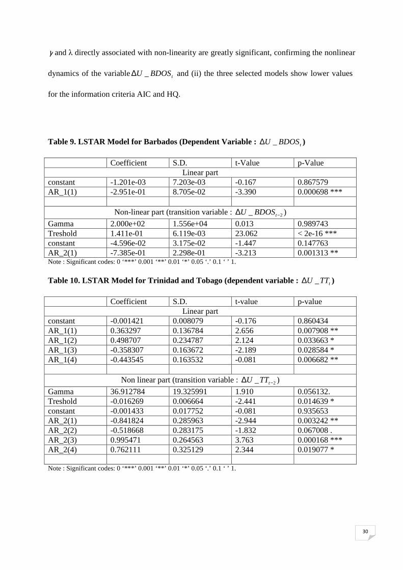
γ and λ directly associated with non-linearity are greatly significant, confirming the nonlinear
dynamics of the variable tBDOSU _∆ and (ii) the three selected models show lower values
for the information criteria AIC and HQ.
Table 9. LSTAR Model for Barbados (Dependent Variable : tBDOSU _∆ ) Coefficient S.D. t-Value p-Value
Linear part constant -1.201e-03 7.203e-03 -0.167 0.867579 AR_1(1) -2.951e-01 8.705e-02 -3.390 0.000698 ***
Non-linear part (transition variable : 2_ −∆ tBDOSU )
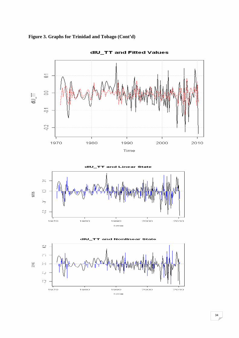
Gamma 2.000e+02 1.556e+04 0.013 0.989743 Treshold 1.411e-01 6.119e-03 23.062 < 2e-16 *** constant -4.596e-02 3.175e-02 -1.447 0.147763 AR_2(1) -7.385e-01 2.298e-01 -3.213 0.001313 ** Note : Significant codes: 0 ‘***’ 0.001 ‘**’ 0.01 ‘*’ 0.05 ‘.’ 0.1 ‘ ’ 1. Table 10. LSTAR Model for Trinidad and Tobago (dependent variable : tTTU _∆ ) Coefficient S.D. t-value p-value
Linear part constant -0.001421 0.008079 -0.176 0.860434 AR_1(1) 0.363297 0.136784 2.656 0.007908 ** AR_1(2) 0.498707 0.234787 2.124 0.033663 * AR_1(3) -0.358307 0.163672 -2.189 0.028584 * AR_1(4) -0.443545 0.163532 -0.081 0.006682 **
Non linear part (transition variable : 2_ −∆ tTTU )
Gamma 36.912784 19.325991 1.910 0.056132. Treshold -0.016269 0.006664 -2.441 0.014639 * constant -0.001433 0.017752 -0.081 0.935653 AR_2(1) -0.841824 0.285963 -2.944 0.003242 ** AR_2(2) -0.518668 0.283175 -1.832 0.067008 . AR_2(3) 0.995471 0.264563 3.763 0.000168 *** AR_2(4) 0.762111 0.325129 2.344 0.019077 * Note : Significant codes: 0 ‘***’ 0.001 ‘**’ 0.01 ‘*’ 0.05 ‘.’ 0.1 ‘ ’ 1.
31
Figure 3. Graphs for Barbados
32
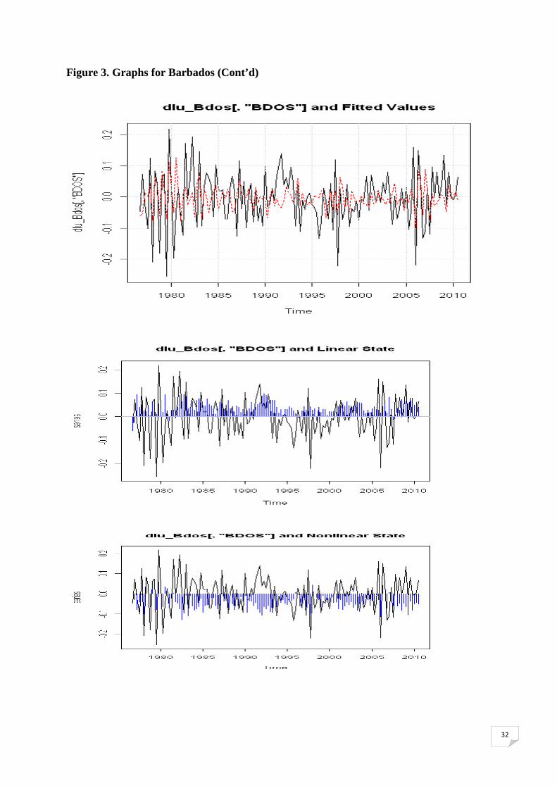
Figure 3. Graphs for Barbados (Cont’d)
33
Figure 4. Graphs for Trinidad and Tobago
34
Figure 3. Graphs for Trinidad and Tobago (Cont’d)
35
Conclusion For several decades, unemployment has emerged as one of the important concerns of policy
makers in many countries of the Caribbean Basin. With values of the rate of unemployment
that can represent up to twice the levels in the OECD and other European countries, the
identification and implementation arrangements for employment is of an even higher priority
in these countries as the performance of their labor markets is often considered to be very
poor. Faced with this situation, it is surprising to note the inadequate number of
comprehensive studies on the characteristics and modeling of unemployment in the
Caribbean.
To contribute to the literature on this topic, this article proposes an econometric analysis of
the phenomenon of hysteresis in unemployment through the modeling of high frequency time
series data. On this basis quarterly unemployment rates for Barbados and Trinidad and
Tobago are the indicators selected over the post 1970 period. The existence of a unit root in
these series are checked and the results confirmed the hypothesis of hysteresis demonstrated
in previous studies, with shocks to the level of unemployment rates that have a lasting effect
in their developments. Next, it is shown that the non-linear processes like the STAR model
are more appropriate than the linear AR models to reproduce the asymmetry and persistence
characterizing unemployment data in the two Caribbean countries examined. More
specifically, the rejection of the assumption of linearity in favor of the alternative non-linear
STAR is highlighted and the superiority of the latter relative to linear models. Also the paper
demonstrates the existence of two equilibria in the dynamic series of differentiated rates of
unemployment and the relatively rapid transition from one regime to another.
36
References
Ball L., HofstetterM. (2009), Unemployment in Latin America and the Caribbean, Working Paper, October, Universidad de los Andes. Borda P. (2000), De l’effet d’hystérèse sur le taux de chômage en Guadeloupe, in Maurin A. et Montauban J-G., « Exclusion, croissance et développement. La Guadeloupe entre défis, incertitudes et espoirs », Economica, 2000. Borda P., Mamingi N., (2009), Structural Shocks and Labour Market Dynamics in a Small Open-Economy: Theory and Some Evidence, Caribbean Centre for Money and Finance, 41st Annual Monetary Studies Conference, 10-13 November 2009, Georgetown Guyana. Blanchard OJ. et Summers L.H. (1986) «Hystérésis and the European Unemployment Problem», NBER Macroeconomics Annual 1986, Cambridge:MIT Press. Blanchard, O. (2005) : «European Unemployment : The Evolution of Facts and Ideas», NBER Working Paper Series n°11750. Cuestas J. and Gil-Alana L.A., (2011), Unemployment hysteresis, structural changes, non-linearities and fractional integration in European transition economies, Sheffield Economic Research Paper Series, University of Sheffield, United Kingdom. Cheng-Feng Lee (2010), Testing for unemployment hysteresis in nonlinear heterogeneous panels: International evidence , Economic Modelling, Volume 27, Issue 5, September 2010, Pages 1097-1102
Elmeçkov J. et MacFarlan M. (1993), Persistance du chômage, Revue économique de l’OCDE. no 21. hiver 1993. Fouquau J. (2008), Modèles à changements de régimes et données de panel : de la non-linéarité à l’hétérogénéité, Thèse de doctorat, UNIVERSITÉ D’ORLÉANS. Franses P.H. (2004), Time series models for business and economic forecasting, Cambridge. Granger, C. W. J. et T. Teräsvirta (1993), Modelling Nonlinear EconomicRelationships, Oxford University Press, Oxford. Kapetanios, G., A. Snell and Y. Shin (2003) “Testing for unit root in the nonlinear STAR framework” Journal of Econometrics 112, 359-379. MacKinnon, James G. (1996). “Numerical Distribution Functions for Unit Root and Cointegration Tests,” Journal of Applied Econometrics, 11, 601-618. Elna Moolman, Asymetric in the cyclical behavior of the South African labor market, South African Journal of Labour Relations: Autumn 2003. Maddala, G. S. (1991), « Disequilibrium Modeling, Switching Regressions, and their Relationship to Structural Change », in P. Hackl et A. H. Westlund (éds), Economic
37
Structural Change : Analysis and Forecasting, Springer, New York, Berlin, London et Tokyo, p. 159-168. Neftçi, S. (1984), ‘Are economic time series asymmetric over the businees cycle ?’, Journal of Political Economy 92(2), 307–328. Louis Phaneuf (1988), « Hystérésis du chômage : Faits, théories et politiques », L'Actualité économique, vol. 64, n° 4, 1988, p. 509-531. Rothman, P. (1991), ‘Further evidence on the asymmetric behaviour of unemployement rates over the business cycle’, Journal of Macroeconometrics 13, 291–298. Teräsvirta, T. (1994), « Specification, Estimation, and Evaluation of Smooth Transition Autoregressive Models », Journal of the American Statistical Association, 89 : 208-218. Teräsvirta, T. et H. M. Anderson (1992), « Characterizing Nonlinearities in Business Cycles Using Smooth Transition Autoregressive Models », Journal of Applied Econometrics, 7 : S119-S136. Sidiropoulos et Trabelsi J. (2001), Les chocs monétaires et la persistance du taux de chômage, Économie et Prévision, n°148 2001-2. Trabelsi J. (1997), Les tests de racine unitaire et les modèles Arch : application au taux de chômage, Economie et Prévision, n°131, 1997-5. Uctum R. (2007), Econométrie des modèles à changement de régimes : un essai de synthèse, L’actualité économique, 2007.

38
Appendix
Table 1. Annual unemployment rate of some Caribbean Basin countries
PAYS Jamaica Dominican Republic
1970
1971
1972 23.2
1973 21.9
1974 20.5
1975 20.4
1976 22.4
1977 24.2
1978 24.3
1979 27.5
1980 27.3
1981 26.0
1982 27.6
1983 26.4
1984 25.6
1985 25.0
1986 23.7
1987 21.0
1988 18.9
1989 16.8
1990 15.7
1991 15.7 19.6
1992 15.4 20.3
1993 16.3 19.9
1994 15.4 16.0
1995 16.2 15.8
1996 16.0 16.7
1997 16.5 16.0
1998 15.5 14.4
1999 15.7 13.8
2000 15.5 13.9
2001 15.0 15.6
2002 14.2 16.1
2003 11.4 17.0
2004 11.7 18.4
2005 11.2 17.9
2006 10.3 16.2
2007 9.8
Source : See Ball L and Hofstetter (2009)
39
Table 2. Standardized unemployment rates in OECD countries, average annual
Country United States Japan Germany UK Italy France Austria Belgium Denmark Finland
1970 4.9 1.1 0.6 2.2 5.5 2.2 1.4 1.9 0.7 1.9
1971 5.9 1.2 0.7 2.8 5.5 2.4 1.3 1.9 1.1 2.3
1972 5.6 1.4 0.9 3.1 6.4 2.5 1.2 2.4 1.0 2.5
1973 4.9 1.3 1.0 2.2 6.4 2.4 1.1 2.5 0.9 2.3
1974 5.6 1.4 2.2 2.1 5.4 2.5 1.3 2.5 3.6 1.7
1975 8.5 1.9 4.0 3.3 5.9 3.6 1.8 4.6 4.9 2.3
1976 7.7 2.0 4.0 4.9 6.8 4.0 1.8 6.0 6.4 3.9
1977 7.1 2.0 3.9 5.2 7.2 4.5 1.6 6.8 7.4 5.9
1978 6.1 2.2 3.7 5.2 7.3 4.7 2.1 7.4 8.4 7.3
1979 5.8 2.1 3.2 4.7 7.8 5.3 2.1 7.7 6.0 6.0
1980 7.1 2.0 3.2 5.7 7.7 5.6 1.9 8.1 6.9 4.7
1981 7.6 2.2 4.6 9.1 8.0 6.6 2.5 10.4 10.4 4.9
1982 9.7 2.4 6.5 10.5 8.7 7.2 3.5 12.2 11.1 5.4
1983 9.6 2.6 8.0 11.4 9.5 7.5 4.1 13.5 11.6 5.5
1984 7.5 2.7 7.2 11.9 10.1 8.7 3.8 13.5 8.6 5.2
1985 7.2 2.6 7.3 11.3 10.4 9.3 3.6 12.6 7.3 5.0
1986 7.0 2.8 6.6 10.8 11.2 9.3 3.1 11.9 5.5 5.4
1987 6.2 2.8 6.3 10.8 12.1 9.5 3.8 11.6 5.5 5.1
1988 5.5 2.5 6.3 8.8 12.1 9.1 3.6 10.5 6.5 4.6
1989 5.3 2.3 5.6 7.2 12.1 8.4 3.1 9.5 8.2 3.1
1990 5.6 2.1 4.8 6.9 11.5 8.1 3.2 8.9 8.4 3.2
1991 6.8 2.1 5.6 8.4 11.0 8.3 3.5 9.5 9.2 6.7
1992 7.5 2.2 6.7 9.7 10.6 9.3 3.6 10.5 9.1 11.7
1993 6.9 2.5 8.0 10.3 10.2 10.4 4.3 12.1 10.8 16.4
1994 6.1 2.9 8.5 9.6 11.2 11.0 3.6 13.1 8.1 16.6
1995 5.6 3.2 8.2 8.6 11.7 10.4 3.7 13.0 7.1 15.4
1996 5.4 3.4 9.0 8.1 11.7 10.9 4.2 12.7 7.0 14.6
1997 4.9 3.4 9.9 7.1 11.8 11.0 4.3 12.6 6.2 12.7
1998 4.5 4.1 9.3 6.1 11.9 10.5 4.3 11.7 5.5 11.4
1999 4.2 4.7 8.5 6.0 11.5 10.1 3.8 8.6 5.6 10.2
2000 4.0 4.7 7.8 5.5 10.7 8.7 3.6 6.6 4.6 9.8
2001 4.7 5.0 7.9 4.8 9.6 7.9 3.7 6.2 4.8 9.1
2002 5.8 5.4 8.6 5.1 9.1 8.0 4.0 6.9 4.8 9.1
2003 6.0 5.3 9.3 4.9 8.8 8.6 4.3 7.7 5.6 9.1
2004 5.5 4.7 10.3 4.7 8.1 9.0 5.0 7.4 5.7 8.8
2005 5.1 4.4 11.2 4.6 7.8 9.0 5.2 8.4 5.0 8.4
2006 4.6 4.1 10.4 5.4 6.9 8.9 4.8 8.2 4.1 7.7
2007 4.6 3.9 8.7 5.3 6.2 8.1 4.4 7.5 4.0 6.9
Source: OECD
40
Table 2(Cont’d). Standardized unemployment rates in OECD countries, average annual
Country Greece Hungary Iceland Ireland Luxembourg Mexico Netherlands Norway Poland Portugal
1970 4.2 - 1.3 5.9 - - 1.0 0.8 - 2.6
1971 3.1 - 0.7 6.9 - - 1.3 0.8 - 2.6
1972 2.1 - 0.5 6.2 - - 2.3 1.7 - 2.6
1973 2.0 - 0.4 5.7 - - 2.3 1.6 - 2.7
1974 2.1 - 0.4 5.4 0.1 - 2.8 1.5 - 1.8
1975 2.3 - 0.5 9.3 0.2 - 5.3 2.3 - 4.6
1976 1.9 - 0.5 9.1 0.3 - 5.6 1.8 - 6.4
1977 1.7 - 0.3 8.8 0.5 - 5.5 1.5 - 7.5
1978 1.8 - 0.3 8.3 0.8 - 5.4 1.8 - 8.1
1979 1.9 - 0.4 6.8 0.7 - 5.5 2.0 - 8.2
1980 2.8 - 0.3 7.4 0.7 - 6.2 1.7 - 7.8
1981 4.0 - 0.4 10.5 1.0 - 8.6 2.1 - 7.6
1982 5.8 - 0.7 11.6 1.3 - 11.6 2.7 - 7.5
1983 7.9 - 1.0 14.0 1.6 - 12.0 3.5 - 7.9
1984 8.1 - 1.3 15.6 1.7 - 12.2 3.2 - 8.5
1985 7.8 - 0.9 16.7 1.6 - 11.1 2.6 - 8.7
1986 7.4 - 0.7 17.1 1.4 - 10.5 2.0 - 8.6
1987 7.4 - 0.4 17.0 1.6 - 9.7 2.1 - 7.1
1988 7.7 - 0.6 16.4 1.4 - 9.3 3.2 - 5.8
1989 7.5 - 1.7 15.2 1.3 - 8.4 5.0 - 5.1
1990 7.0 - 1.8 13.0 1.1 2.7 7.6 5.3 6.5 4.6
1991 7.7 - 2.5 14.8 1.2 3.0 7.1 5.6 12.3 4.3
1992 8.7 9.9 4.3 15.2 1.3 3.1 6.8 6.0 13.3 4.1
1993 9.7 12.1 5.3 15.8 1.7 3.2 6.2 6.1 14.0 5.5
1994 9.6 11.0 5.3 14.8 2.1 3.5 6.9 5.5 14.4 6.8
1995 10.0 10.4 4.9 12.2 2.3 6.9 7.1 5.0 13.3 7.2
1996 10.3 10.1 3.7 11.9 2.5 5.2 6.5 4.9 12.4 7.2
1997 10.2 8.9 3.9 10.4 2.7 4.1 5.5 4.1 11.2 6.7
1998 10.8 7.9 2.7 7.8 2.3 3.6 4.3 3.2 10.5 5.0
1999 11.9 7.1 2.0 5.8 2.1 2.5 3.5 3.2 13.9 4.4
2000 11.2 6.5 2.3 4.3 1.9 2.6 2.7 3.5 16.1 4.0
2001 10.4 5.8 2.3 3.7 1.7 2.5 2.1 3.6 18.2 4.1
2002 9.9 5.9 3.3 4.2 2.0 2.9 2.6 3.9 19.9 5.1
2003 9.3 5.9 3.4 4.4 2.5 3.0 3.6 4.5 19.6 6.4
2004 10.2 6.2 3.1 4.4 2.8 3.7 4.6 4.5 19.0 6.7
2005 9.6 7.3 2.6 4.3 3.1 3.5 4.7 4.6 17.7 7.7
2006 8.8 7.5 2.9 4.4 3.1 3.2 3.9 3.5 13.8 7.7
2007 8.1 7.4 2.3 4.6 3.0 3.4 3.2 2.5 9.6 8.0
Source: OECD
41
Table 2 (Cont’d). Standardized unemployment rates in OECD countries, average annual
PAYS Slovak
Republic Spain Sweden Switzerland Turkey Australia Canada South Korea
New Zealand
OECD Total
1970 - 1.5 1.5 - 6.3 1.4 5.7 4.4 0.1 -
1971 - 2.0 2.5 - 6.6 1.7 6.2 4.4 0.2 -
1972 - 3.0 2.7 - 6.2 2.5 6.2 4.5 0.5 -
1973 - 2.7 2.5 - 6.6 1.8 5.6 3.9 0.2 -
1974 - 3.2 2.0 - 7.2 2.4 5.3 4.0 0.1 -
1975 - 4.7 1.6 0.3 7.4 4.5 6.9 4.1 0.2 -
1976 - 4.6 1.7 0.7 8.8 4.7 7.1 3.9 0.3 -
1977 - 5.2 2.0 0.4 9.8 5.6 8.0 3.8 0.3 -
1978 - 7.0 2.5 0.3 9.9 6.2 8.4 3.2 1.7 -
1979 - 8.7 2.3 0.3 8.7 6.3 7.5 3.8 1.9 -
1980 - 11.5 2.2 0.2 8.1 6.1 7.5 5.2 2.2 -
1981 - 14.2 2.8 0.2 7.1 5.8 7.6 4.5 3.6 -
1982 - 16.0 3.5 0.4 7.0 7.2 11.0 4.4 3.6 -
1983 - 17.5 3.9 0.9 7.7 10.0 12.0 4.1 5.7 -
1984 - 20.2 3.5 1.1 7.6 9.0 11.3 3.8 5.7 -
1985 - 21.6 3.1 0.9 7.1 8.3 10.6 4.0 4.2 -
1986 - 21.1 2.9 0.8 7.9 8.1 9.7 3.8 4.1 -
1987 - 20.3 2.3 0.7 8.3 8.1 8.8 3.1 4.1 -
1988 - 19.3 1.9 0.6 8.4 7.2 7.8 2.5 5.6 -
1989 - 17.3 1.6 0.5 8.6 6.2 7.5 2.6 7.1 -
1990 - 16.3 1.8 0.5 8.0 6.9 8.1 2.4 7.8 -
1991 - 16.4 3.3 1.8 8.2 9.6 10.3 2.4 10.3 -
1992 - 18.5 5.8 2.8 8.5 10.8 11.2 2.5 10.4 -
1993 - 22.8 9.5 3.8 8.9 10.9 11.4 2.9 9.5 -
1994 13.6 24.2 9.8 3.7 8.6 9.7 10.4 2.5 8.1 7.6
1995 13.1 23.0 9.2 3.4 7.6 8.5 9.5 2.1 6.3 7.4
1996 11.3 22.1 10.0 3.7 6.6 8.5 9.6 2.0 6.1 7.3
1997 11.9 20.7 10.2 4.1 6.8 8.5 9.1 2.6 6.6 7.0
1998 12.6 18.7 8.5 3.4 6.9 7.7 8.3 7.0 7.4 6.8
1999 16.4 15.7 7.2 2.9 7.7 6.9 7.6 6.3 6.8 6.6
2000 18.8 13.9 5.9 2.6 6.5 6.3 6.8 4.4 6.0 6.1
2001 19.3 10.6 5.1 2.5 8.4 6.8 7.2 4.0 5.3 6.2
2002 18.6 11.5 5.2 3.0 10.3 6.4 7.7 3.3 5.2 6.8
2003 17.5 11.5 5.8 4.0 10.5 6.1 7.6 3.6 4.6 6.9
2004 18.1 11.0 6.6 4.2 10.3 5.5 7.2 3.7 3.9 6.8
2005 16.2 9.2 7.8 4.3 10.3 5.1 6.8 3.7 3.7 6.6
2006 13.3 8.5 7.1 3.9 9.9 4.9 6.3 3.5 3.8 6.1
2007 11.0 8.3 6.2 3.5 9.9 4.4 6.0 3.2 3.6 5.6
Source: OECD