Embed Size (px)
Citation preview
Understanding Variation
that Extends
Statistical Process Control
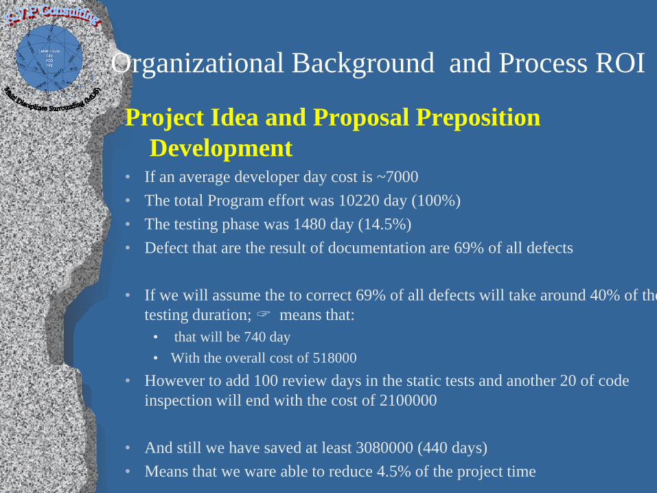
Organizational Background and Process ROI
Project Idea and Proposal Preposition Development
• If an average developer day cost is ~7000 • The total Program effort was 10220 day (100%) • The testing phase was 1480 day (14.5%) • Defect that are the result of documentation are 69% of all defects
• If we will assume the to correct 69% of all defects will take around 40% of the
testing duration; means that: • that will be 740 day • With the overall cost of 518000
• However to add 100 review days in the static tests and another 20 of code inspection will end with the cost of 2100000
• And still we have saved at least 3080000 (440 days) • Means that we ware able to reduce 4.5% of the project time

Our Business Process
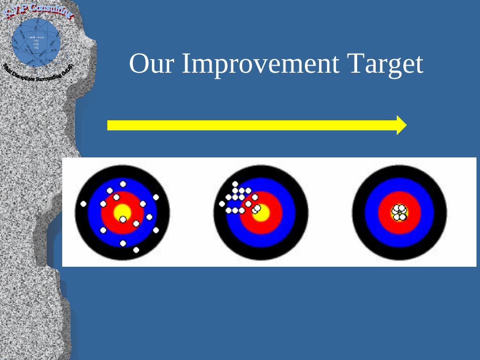
Our Improvement Target
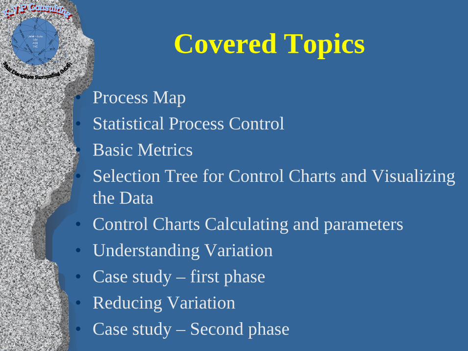
Covered Topics
• Process Map • Statistical Process Control • Basic Metrics • Selection Tree for Control Charts and Visualizing
the Data • Control Charts Calculating and parameters • Understanding Variation • Case study – first phase • Reducing Variation • Case study – Second phase
6
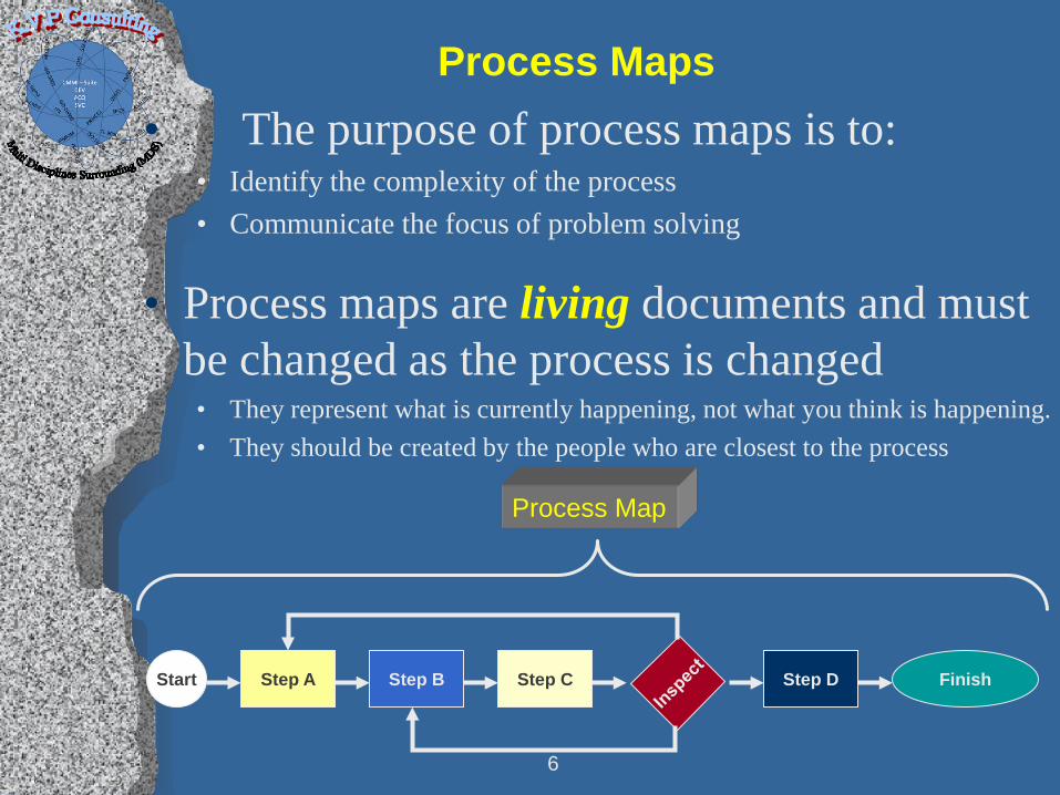
Process Maps • The purpose of process maps is to:
• Identify the complexity of the process • Communicate the focus of problem solving
• Process maps are living documents and must be changed as the process is changed
• They represent what is currently happening, not what you think is happening. • They should be created by the people who are closest to the process
Step A Start Finish Step B Step C Step D
Process Map
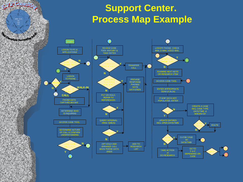
Support Center. Process Map Example
START
LOGON TO PC & APPLICATIONS
SCHEDULED PHONE TIME?
LOGON TO PHONE
CALL or WALK-IN?
PHONE DATA CAPTURE BEGINS
DETERMINE WHO IS INQUIRING
ACCESS CASE TOOL
CASE TOOL RECORD?
Y
N
A
Z
CALL
WALK-IN
DETERMINE NATURE OF CALL & CONFIRM
UNDERSTANDING
Y
N C
B
D PHONE TIME
Y
N
Z
B
C
REVIEW CASE TOOL HISTORY &
TAKE NOTES
PUT ON HOLD, REFER TO
REFERENCES
IMMEDIATE RESPONSE AVAILABLE?
Y
N
TRANSFER APPROPRIATE?
Y
N
TRANSFER CALL
ANSWER? Y
N
QUERY INTERNAL HRSC SME(S)
ANSWER? Y
N OFF HOLD AND ARRANGE CALL
BACK PHONE DATA ENDS
PROVIDE RESPONSE
PHONE& NOTE
DATA ENDS
D
ADD TO RESEARCH
LIST
Z
LOGOFF PHONE, CHECK MAIL,E-MAIL,VOICE MAIL
SCHEDULED PHONE TIME?
N
Y A
E
EXAMINE NEXT NOTE OR RESEARCH ITEM
ACCESS CASE TOOL
ENTER APPROPRIATE SSAN (#,9s,0s)
IF EMP DATA NOT POPULATED, ENTER
OLD CASE
Y
N
UPDATE ENTRIES INCL OPEN DATE/TIME
CREATE A CASE INCL CASE TYPE
DATE/TIME, & NEEDED BY
AUTO ROUTE
Y ROUTE
CASE CLOSED
N
Y
N
CLOSE CASE W/
DATE/TIME E
TAKE ACTION or
DO RESEARCH
F
GO TO F or E
DEPENDING ON CASE F
E NEXT
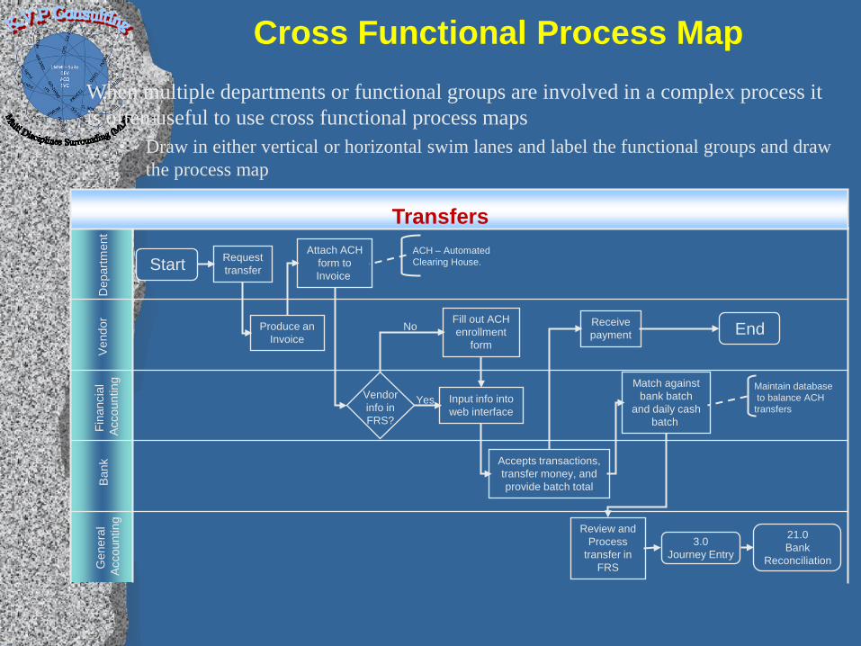
Cross Functional Process Map When multiple departments or functional groups are involved in a complex process it is often useful to use cross functional process maps
• Draw in either vertical or horizontal swim lanes and label the functional groups and draw the process map
Gen
eral
Ac
coun
ting
Bank
Fi
nanc
ial
Acco
untin
g Ve
ndor
D
epar
tmen
t
Start Request transfer
Attach ACH form to Invoice
Produce an Invoice
Fill out ACH enrollment
form
Receive payment End
Vendor info in FRS?
Input info into web interface
Match against bank batch
and daily cash batch
Accepts transactions, transfer money, and provide batch total
Review and Process
transfer in FRS
3.0 Journey Entry
21.0 Bank
Reconciliation
Maintain database to balance ACH transfers
ACH – Automated Clearing House.
No
Yes
Transfers
STATISTICAL PROCESS CONTROL
10 Control Phase
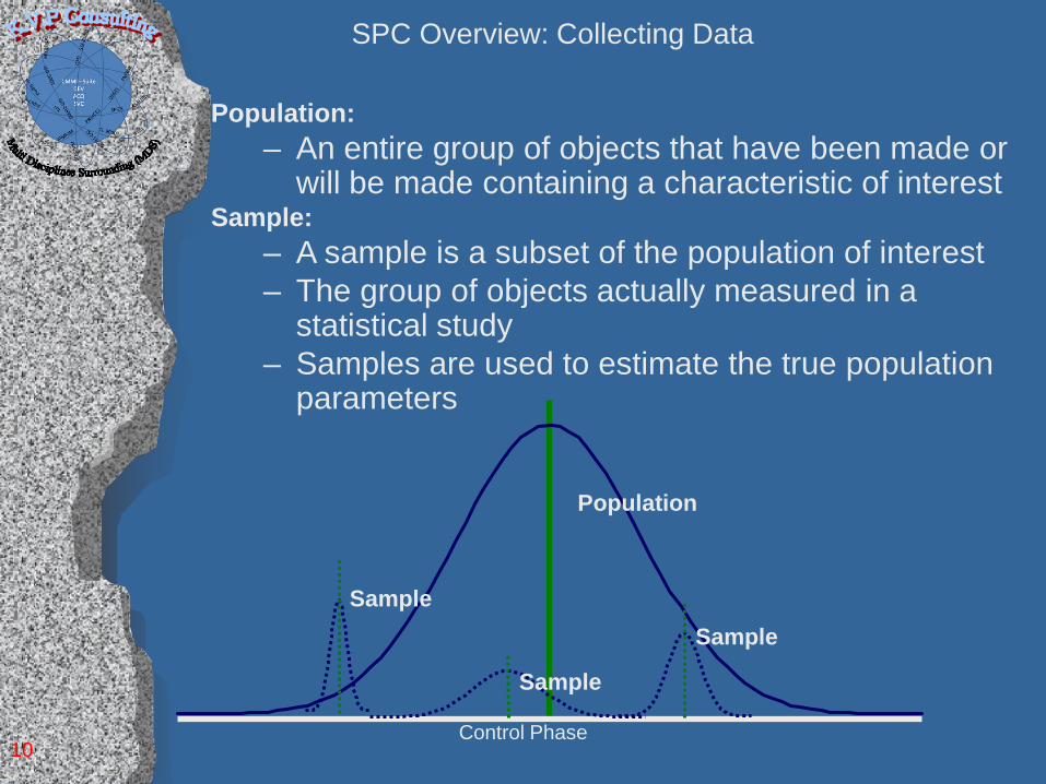
SPC Overview: Collecting Data
Population: – An entire group of objects that have been made or
will be made containing a characteristic of interest Sample:
– A sample is a subset of the population of interest – The group of objects actually measured in a
statistical study – Samples are used to estimate the true population
parameters
Population
Sample
Sample
Sample
Purpose of Statistical Process Control Every process has Causes of Variation known as:
• Common Cause: Natural variability • Special Cause: Unnatural variability
• Assignable: Reason for detected Variability • Pattern Change: Presence of trend or unusual
pattern
SPC is a basic tool to monitor and improve variation in a process.
SPC is used to detect special cause variation telling us the process is “out of control” but does NOT tell us why.
SPC gives a glimpse of ongoing process capability AND is a visual management tool.
Observation
Indi
vidu
al V
alue
28252219161310741
60
50
40
30
20
10
0
_X=29.06
UCL=55.24
LCL=2.87
1
Control Chart of Recycle
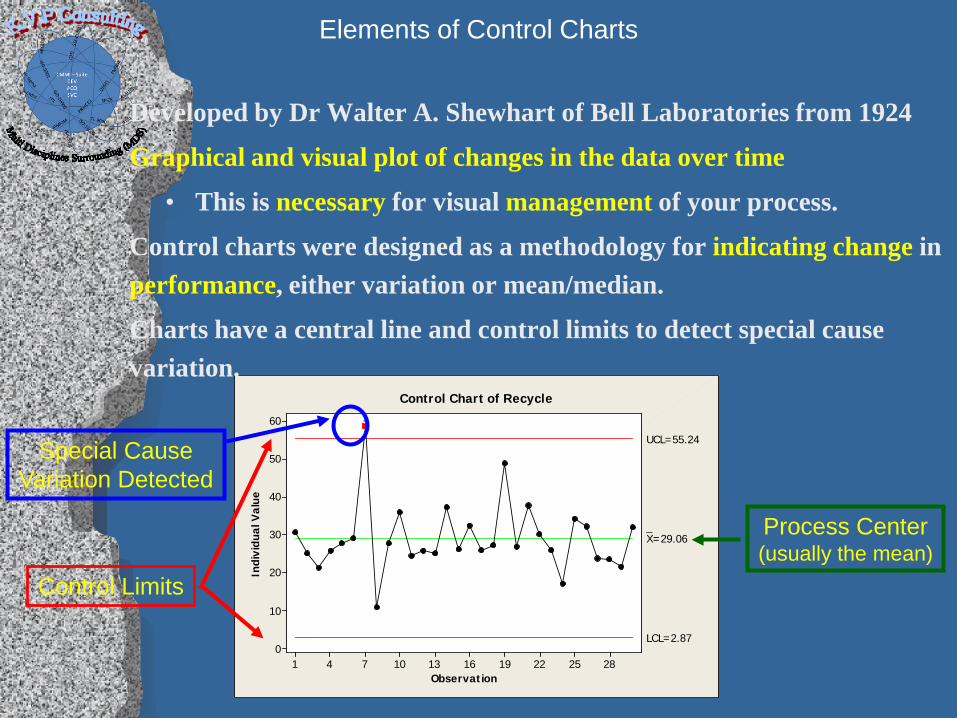
Elements of Control Charts
Developed by Dr Walter A. Shewhart of Bell Laboratories from 1924
Graphical and visual plot of changes in the data over time
• This is necessary for visual management of your process.
Control charts were designed as a methodology for indicating change in performance, either variation or mean/median.
Charts have a central line and control limits to detect special cause variation.
Process Center (usually the mean)
Special Cause Variation Detected
Control Limits
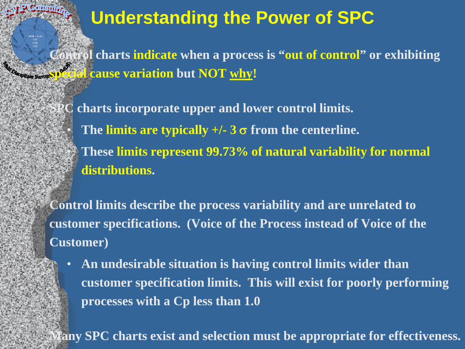
Understanding the Power of SPC
Control charts indicate when a process is “out of control” or exhibiting special cause variation but NOT why!
SPC charts incorporate upper and lower control limits.
• The limits are typically +/- 3 σ from the centerline.
• These limits represent 99.73% of natural variability for normal distributions.
Control limits describe the process variability and are unrelated to customer specifications. (Voice of the Process instead of Voice of the Customer)
• An undesirable situation is having control limits wider than customer specification limits. This will exist for poorly performing processes with a Cp less than 1.0
Many SPC charts exist and selection must be appropriate for effectiveness.

General Steps for Constructing Control Charts
• Select characteristic (critical “X” or CTQ) to be charted. • Determine the purpose of the chart. • Select data-collection points. • Establish the basis for sub-grouping (only for Y’s). • Select the type of control chart. • Determine the measurement method/criteria. • Establish the sampling interval/frequency. • Determine the sample size. • Establish the basis of calculating the control limits. • Set up the forms or software for charting data. • Set up the forms or software for collecting data. • Prepare written instructions for all phases. • Conduct the necessary training.
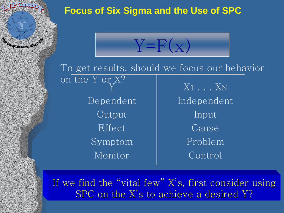
To get results, should we focus our behavior on the Y or X?
Y
Dependent
Output
Effect
Symptom
Monitor
X1 . . . XN
Independent
Input
Cause
Problem
Control
If we find the “vital few” X’s, first consider using SPC on the X’s to achieve a desired Y?
Y=F(x)
Focus of Six Sigma and the Use of SPC
BASIC METRICS
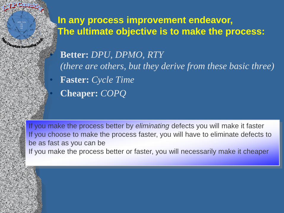
• Better: DPU, DPMO, RTY
(there are others, but they derive from these basic three) • Faster: Cycle Time • Cheaper: COPQ
In any process improvement endeavor, The ultimate objective is to make the process:
If you make the process better by eliminating defects you will make it faster If you choose to make the process faster, you will have to eliminate defects to be as fast as you can be If you make the process better or faster, you will necessarily make it cheaper
Cycle Time Defined
Think of Cycle Time in terms of your product or transaction in the eyes of the customer of the process:
• It is the time required for the product or transaction to
go through the entire process, from beginning to end
• It is not simply the “touch time” of the value-added portion of the process
What is the cycle time of the process you mapped?
Is there any variation in the cycle time? Why?
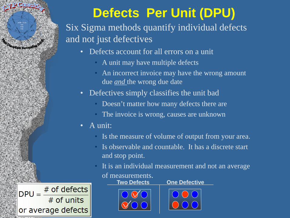
Defects Per Unit (DPU) Six Sigma methods quantify individual defects and not just defectives
• Defects account for all errors on a unit • A unit may have multiple defects • An incorrect invoice may have the wrong amount
due and the wrong due date • Defectives simply classifies the unit bad
• Doesn’t matter how many defects there are • The invoice is wrong, causes are unknown
• A unit: • Is the measure of volume of output from your area. • Is observable and countable. It has a discrete start
and stop point. • It is an individual measurement and not an average
of measurements. Two Defects One Defective
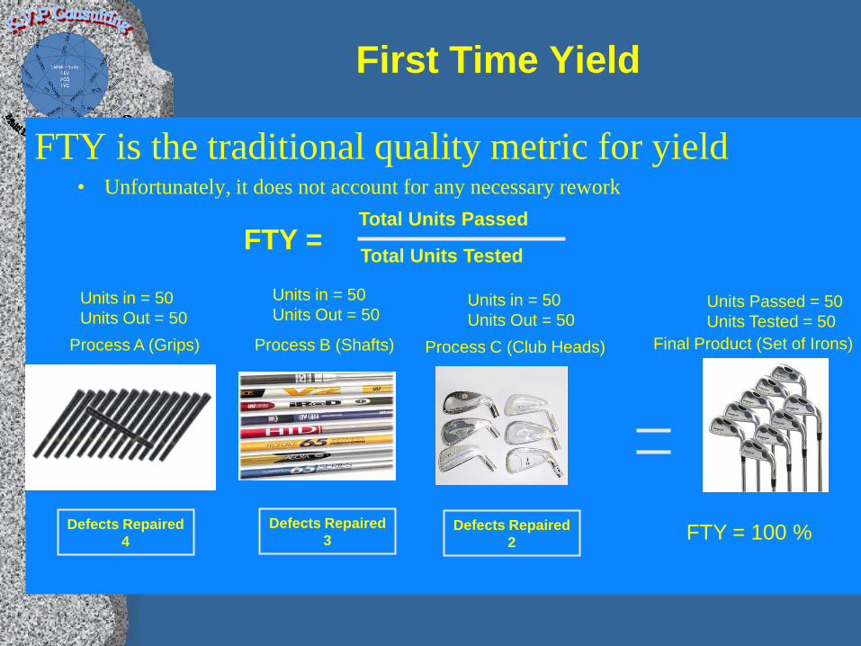
First Time Yield
FTY is the traditional quality metric for yield • Unfortunately, it does not account for any necessary rework
FTY = Total Units Passed
Total Units Tested
Units in = 50 Units Out = 50
Units in = 50 Units Out = 50
Units in = 50 Units Out = 50
Units Passed = 50 Units Tested = 50
FTY = 100 %
Process A (Grips) Process B (Shafts) Process C (Club Heads) Final Product (Set of Irons)
Defects Repaired 4
Defects Repaired 3
Defects Repaired 2
Rolled Throughput Yield
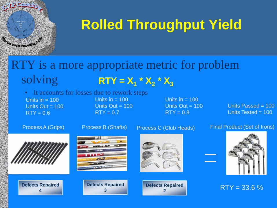
RTY is a more appropriate metric for problem solving • It accounts for losses due to rework steps
RTY = X1 * X2 * X3
Units in = 100 Units Out = 100 RTY = 0.6
Units in = 100 Units Out = 100 RTY = 0.7
Units in = 100 Units Out = 100 RTY = 0.8
Units Passed = 100 Units Tested = 100
RTY = 33.6 %
Process A (Grips) Process B (Shafts) Process C (Club Heads) Final Product (Set of Irons)
Defects Repaired 4
Defects Repaired 3
Defects Repaired 2
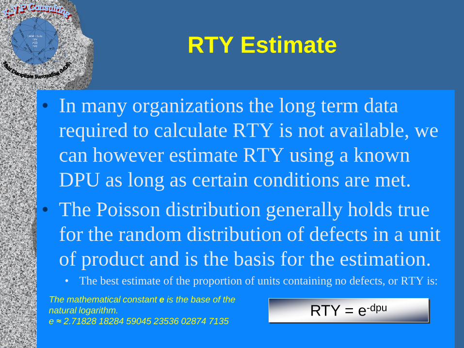
RTY Estimate
• In many organizations the long term data required to calculate RTY is not available, we can however estimate RTY using a known DPU as long as certain conditions are met.
• The Poisson distribution generally holds true for the random distribution of defects in a unit of product and is the basis for the estimation. • The best estimate of the proportion of units containing no defects, or RTY is:
RTY = e-dpu The mathematical constant e is the base of the natural logarithm. e ≈ 2.71828 18284 59045 23536 02874 7135
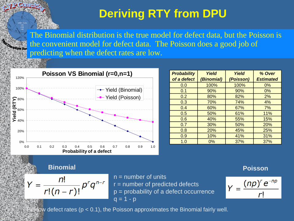
Deriving RTY from DPU
The Binomial distribution is the true model for defect data, but the Poisson is the convenient model for defect data. The Poisson does a good job of predicting when the defect rates are low.
n = number of units r = number of predicted defects p = probability of a defect occurrence q = 1 - p
Poisson VS Binomial (r=0,n=1)
0%
20%
40%
60%
80%
100%
120%
0.0 0.1 0.2 0.3 0.4 0.5 0.6 0.7 0.8 0.9 1.0Probability of a defect
Yiel
d (R
TY)
Yield (Binomial)Yield (Poisson)
For low defect rates (p < 0.1), the Poisson approximates the Binomial fairly well.
Binomial Poisson
Probability of a defect
Yield (Binomial)
Yield (Poisson)
% Over Estimated
0.0 100% 100% 0%0.1 90% 90% 0%0.2 80% 82% 2%0.3 70% 74% 4%0.4 60% 67% 7%0.5 50% 61% 11%0.6 40% 55% 15%0.7 30% 50% 20%0.8 20% 45% 25%0.9 10% 41% 31%1.0 0% 37% 37%
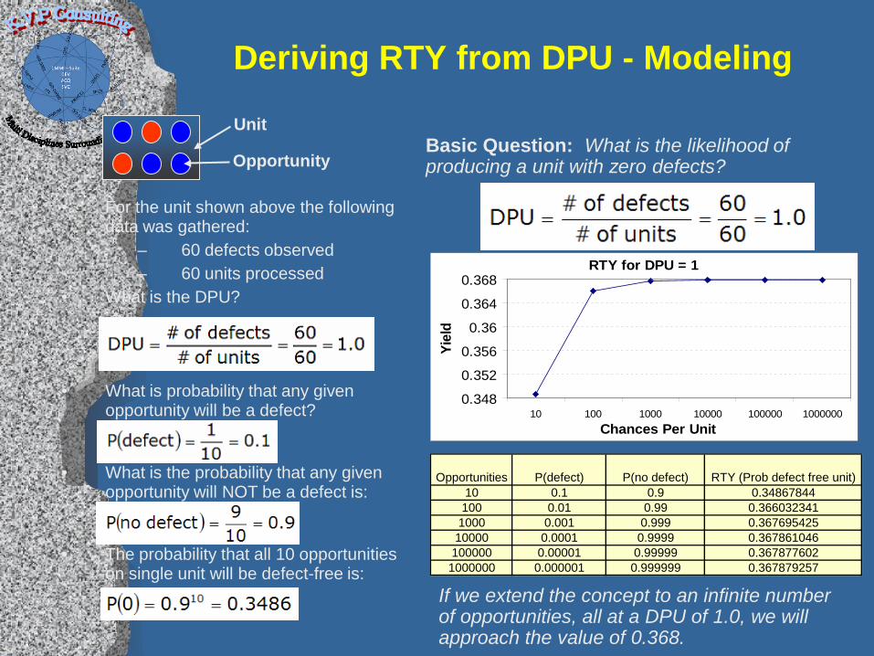
Deriving RTY from DPU - Modeling
• For the unit shown above the following
data was gathered: – 60 defects observed – 60 units processed
• What is the DPU?
• What is probability that any given opportunity will be a defect?
• What is the probability that any given opportunity will NOT be a defect is:
• The probability that all 10 opportunities on single unit will be defect-free is:
RTY for DPU = 1
0.348
0.352
0.356
0.36
0.364
0.368
10 100 1000 10000 100000 1000000Chances Per Unit
Yiel
d
Basic Question: What is the likelihood of producing a unit with zero defects?
Unit
Opportunity
Opportunities P(defect) P(no defect) RTY (Prob defect free unit)10 0.1 0.9 0.34867844100 0.01 0.99 0.3660323411000 0.001 0.999 0.36769542510000 0.0001 0.9999 0.367861046100000 0.00001 0.99999 0.3678776021000000 0.000001 0.999999 0.367879257
If we extend the concept to an infinite number of opportunities, all at a DPU of 1.0, we will approach the value of 0.368.
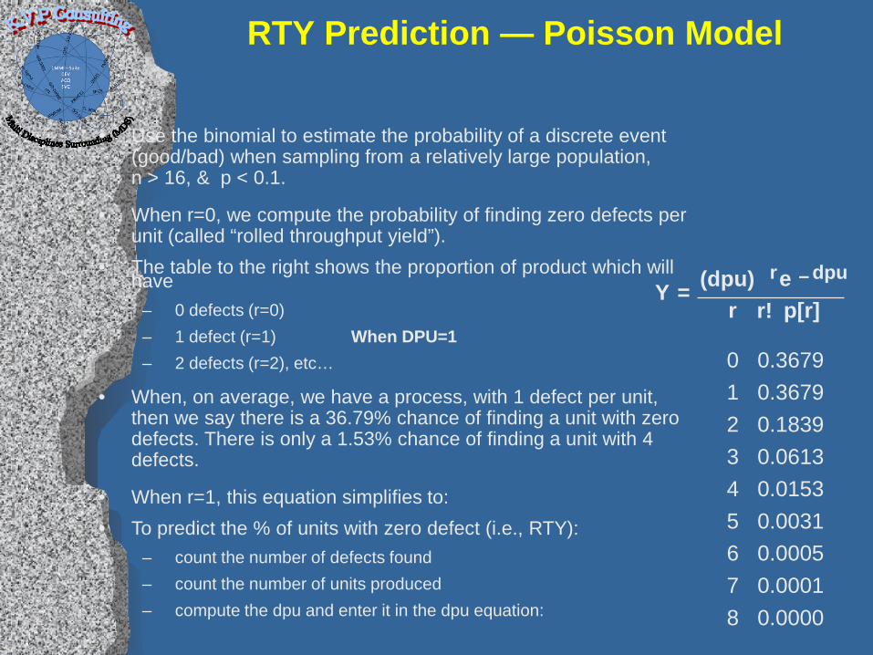
RTY Prediction — Poisson Model
• Use the binomial to estimate the probability of a discrete event (good/bad) when sampling from a relatively large population, n > 16, & p < 0.1.
• When r=0, we compute the probability of finding zero defects per unit (called “rolled throughput yield”).
• The table to the right shows the proportion of product which will have
– 0 defects (r=0) – 1 defect (r=1) When DPU=1 – 2 defects (r=2), etc…
• When, on average, we have a process, with 1 defect per unit, then we say there is a 36.79% chance of finding a unit with zero defects. There is only a 1.53% chance of finding a unit with 4 defects.
• When r=1, this equation simplifies to: • To predict the % of units with zero defect (i.e., RTY):
– count the number of defects found – count the number of units produced – compute the dpu and enter it in the dpu equation:
0 0.3679
1 0.3679
2 0.1839
3 0.0613
4 0.0153
5 0.0031
6 0.0005
7 0.0001
8 0.0000
r p[r] Y = (dpu) r e – dpu
r!
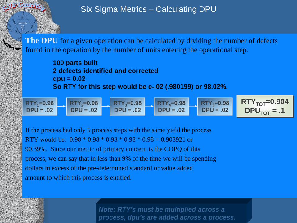
Six Sigma Metrics – Calculating DPU
The DPU for a given operation can be calculated by dividing the number of defects found in the operation by the number of units entering the operational step. If the process had only 5 process steps with the same yield the process RTY would be: 0.98 * 0.98 * 0.98 * 0.98 * 0.98 = 0.903921 or 90.39%. Since our metric of primary concern is the COPQ of this process, we can say that in less than 9% of the time we will be spending dollars in excess of the pre-determined standard or value added amount to which this process is entitled.
RTY1=0.98 DPU = .02
RTY2=0.98 DPU = .02
RTY3=0.98 DPU = .02
RTY4=0.98 DPU = .02
RTY5=0.98 DPU = .02
RTYTOT=0.904 DPUTOT = .1
100 parts built 2 defects identified and corrected dpu = 0.02 So RTY for this step would be e-.02 (.980199) or 98.02%.
Note: RTY’s must be multiplied across a process, dpu’s are added across a process.
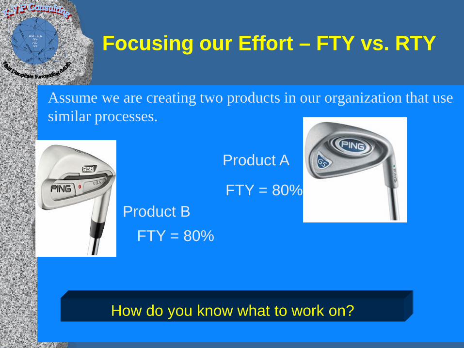
Focusing our Effort – FTY vs. RTY
Assume we are creating two products in our organization that use similar processes.
FTY = 80%
FTY = 80%
How do you know what to work on?
Product A
Product B
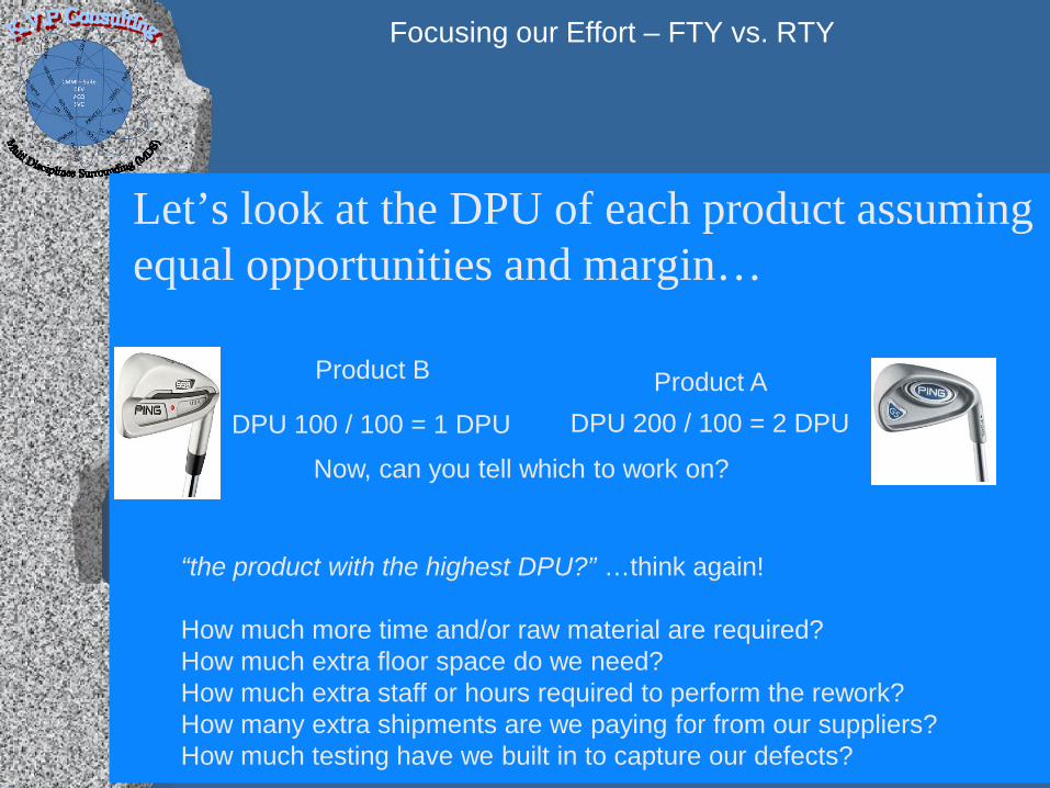
Focusing our Effort – FTY vs. RTY
Let’s look at the DPU of each product assuming equal opportunities and margin…
Product A Product B
DPU 200 / 100 = 2 DPU DPU 100 / 100 = 1 DPU
Now, can you tell which to work on?
“the product with the highest DPU?” …think again! How much more time and/or raw material are required? How much extra floor space do we need? How much extra staff or hours required to perform the rework? How many extra shipments are we paying for from our suppliers? How much testing have we built in to capture our defects?
Selection and Design of Control Charts
Visualizing the Data
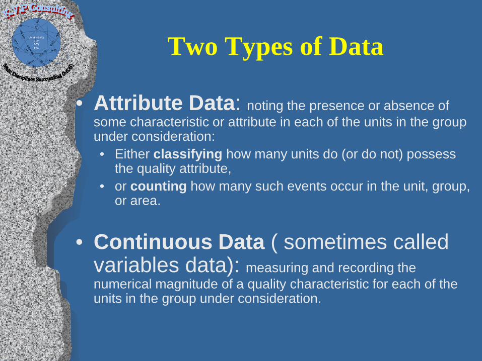
Two Types of Data
• Attribute Data: noting the presence or absence of some characteristic or attribute in each of the units in the group under consideration: • Either classifying how many units do (or do not) possess
the quality attribute, • or counting how many such events occur in the unit, group,
or area.
• Continuous Data ( sometimes called variables data): measuring and recording the numerical magnitude of a quality characteristic for each of the units in the group under consideration.
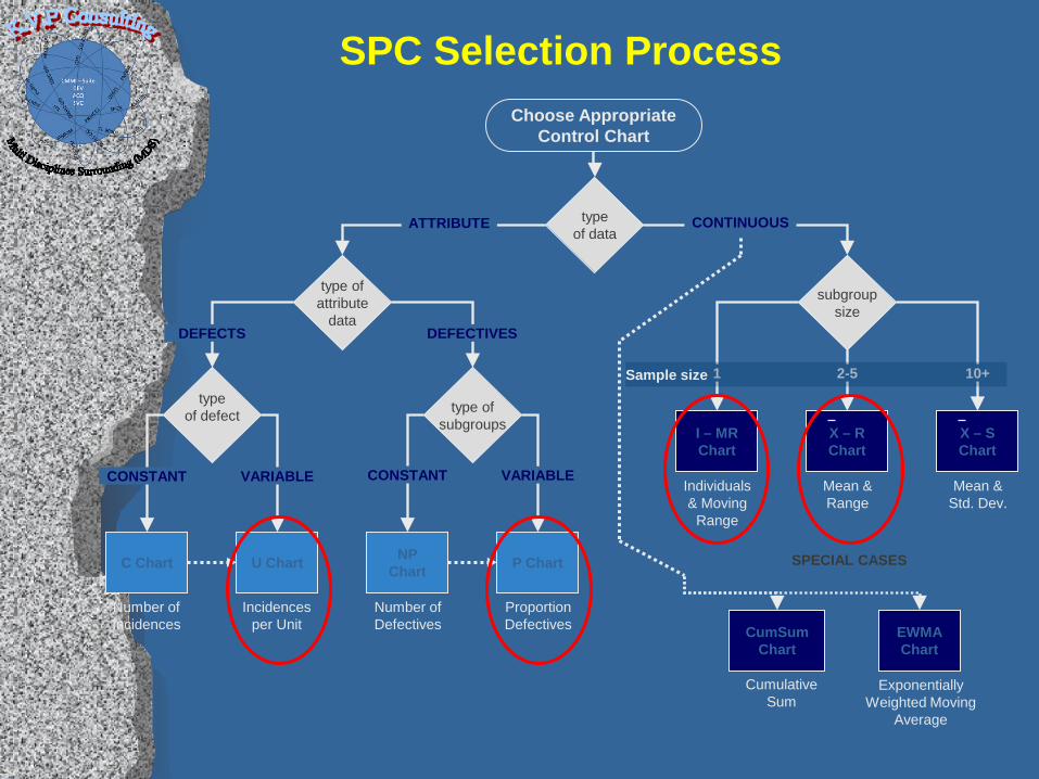
SPC Selection Process Choose Appropriate
Control Chart
type of data
type of attribute
data
subgroup size
I – MR Chart
X – R Chart
X – S Chart
CumSum Chart
EWMA Chart
C Chart U Chart NP Chart P Chart
type of defect
type of subgroups
ATTRIBUTE CONTINUOUS
DEFECTS DEFECTIVES
VARIABLE CONSTANT CONSTANT VARIABLE
1 2-5 10+
Number of Incidences
Incidences per Unit
Number of Defectives
Proportion Defectives
Individuals & Moving
Range
Mean & Range
Mean & Std. Dev.
Cumulative Sum
Exponentially Weighted Moving
Average
SPECIAL CASES
Sample size
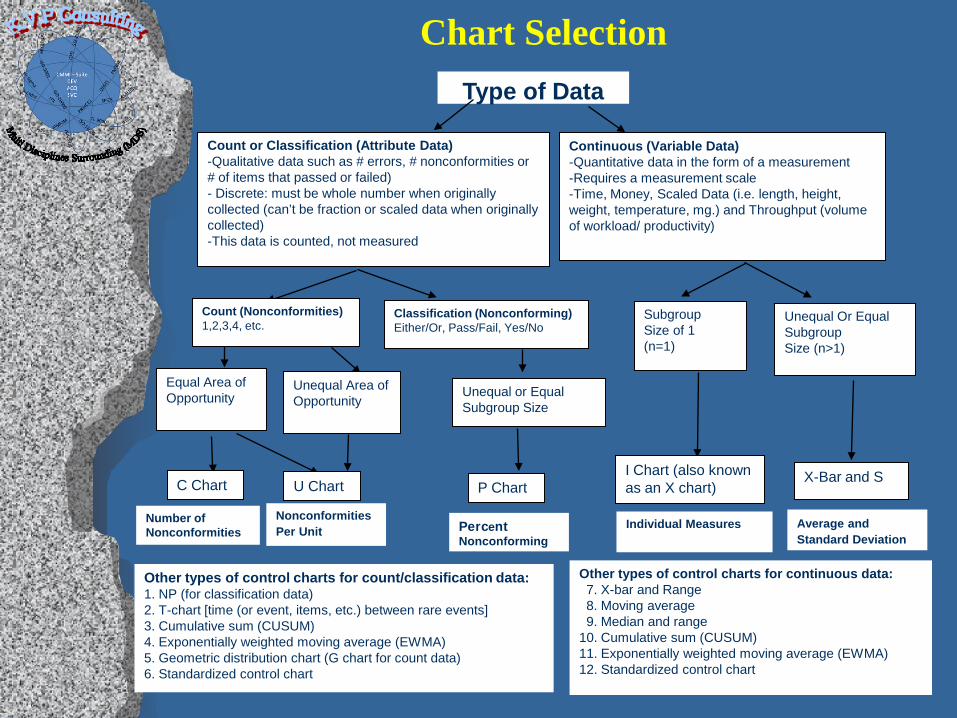
Chart Selection Type of Data
Count or Classification (Attribute Data) -Qualitative data such as # errors, # nonconformities or # of items that passed or failed) - Discrete: must be whole number when originally collected (can’t be fraction or scaled data when originally collected) -This data is counted, not measured
Count (Nonconformities) 1,2,3,4, etc.
Classification (Nonconforming) Either/Or, Pass/Fail, Yes/No
Equal Area of Opportunity
Unequal Area of Opportunity
Unequal or Equal Subgroup Size
Continuous (Variable Data) -Quantitative data in the form of a measurement -Requires a measurement scale -Time, Money, Scaled Data (i.e. length, height, weight, temperature, mg.) and Throughput (volume of workload/ productivity)
Subgroup Size of 1 (n=1)
Unequal Or Equal Subgroup Size (n>1)
C Chart U Chart P Chart I Chart (also known as an X chart)
X-Bar and S
Number of Nonconformities
Nonconformities Per Unit
Percent Nonconforming
Individual Measures
Average and Standard Deviation
Other types of control charts for count/classification data: 1. NP (for classification data) 2. T-chart [time (or event, items, etc.) between rare events] 3. Cumulative sum (CUSUM) 4. Exponentially weighted moving average (EWMA) 5. Geometric distribution chart (G chart for count data) 6. Standardized control chart
Other types of control charts for continuous data: 7. X-bar and Range 8. Moving average 9. Median and range 10. Cumulative sum (CUSUM) 11. Exponentially weighted moving average (EWMA) 12. Standardized control chart
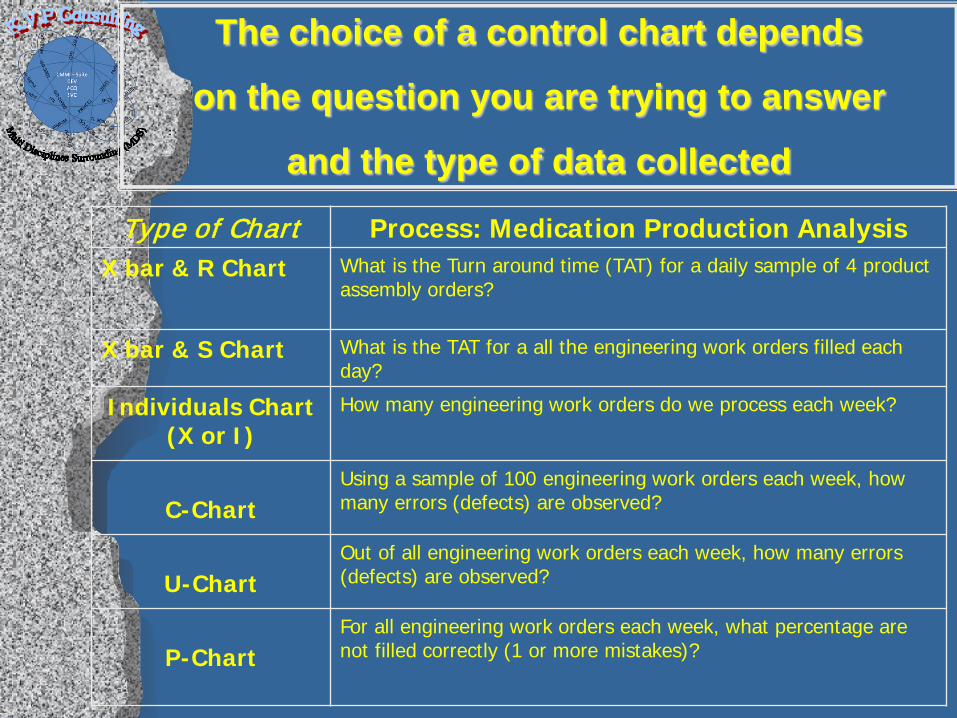
Type of Chart Process: Medication Production Analysis X bar & R Chart What is the Turn around time (TAT) for a daily sample of 4 product
assembly orders?
X bar & S Chart What is the TAT for a all the engineering work orders filled each day?
Individuals Chart (X or I)
How many engineering work orders do we process each week?
C-Chart
Using a sample of 100 engineering work orders each week, how many errors (defects) are observed?
U-Chart
Out of all engineering work orders each week, how many errors (defects) are observed?
P-Chart
For all engineering work orders each week, what percentage are not filled correctly (1 or more mistakes)?
The choice of a control chart depends
on the question you are trying to answer
and the type of data collected
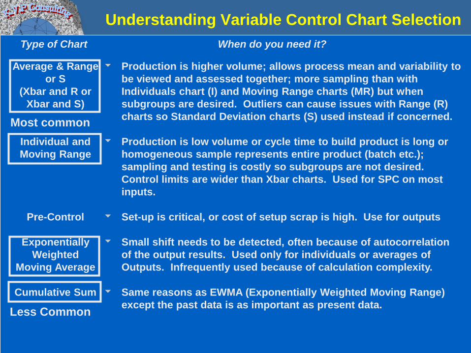
Understanding Variable Control Chart Selection Type of Chart When do you need it?
Production is higher volume; allows process mean and variability to be viewed and assessed together; more sampling than with Individuals chart (I) and Moving Range charts (MR) but when subgroups are desired. Outliers can cause issues with Range (R) charts so Standard Deviation charts (S) used instead if concerned.
Production is low volume or cycle time to build product is long or homogeneous sample represents entire product (batch etc.); sampling and testing is costly so subgroups are not desired. Control limits are wider than Xbar charts. Used for SPC on most inputs.
Set-up is critical, or cost of setup scrap is high. Use for outputs
Small shift needs to be detected, often because of autocorrelation of the output results. Used only for individuals or averages of Outputs. Infrequently used because of calculation complexity.
Same reasons as EWMA (Exponentially Weighted Moving Range) except the past data is as important as present data.
Average & Range or S
(Xbar and R or Xbar and S)
Individual and Moving Range
Pre-Control
Exponentially Weighted
Moving Average
Cumulative Sum
Most common
Less Common
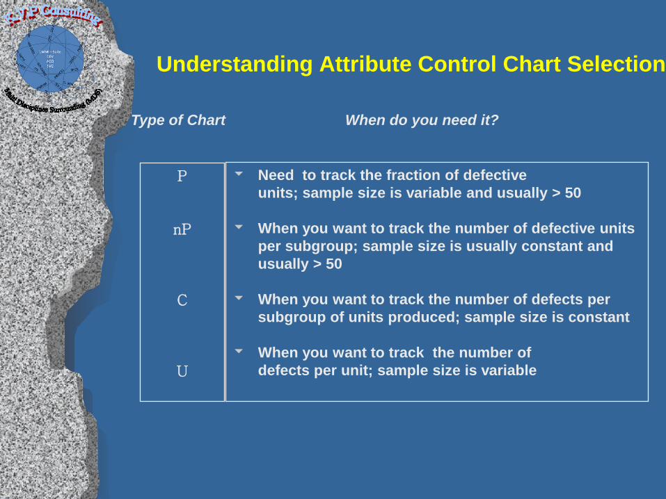
Understanding Attribute Control Chart Selection
Need to track the fraction of defective units; sample size is variable and usually > 50
When you want to track the number of defective units
per subgroup; sample size is usually constant and usually > 50
When you want to track the number of defects per subgroup of units produced; sample size is constant
When you want to track the number of defects per unit; sample size is variable
P
nP
C
U
When do you need it? Type of Chart
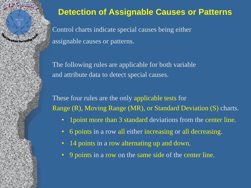
Detection of Assignable Causes or Patterns
Control charts indicate special causes being either
assignable causes or patterns.
The following rules are applicable for both variable and attribute data to detect special causes.
These four rules are the only applicable tests for Range (R), Moving Range (MR), or Standard Deviation (S) charts.
• 1point more than 3 standard deviations from the center line.
• 6 points in a row all either increasing or all decreasing.
• 14 points in a row alternating up and down.
• 9 points in a row on the same side of the center line.
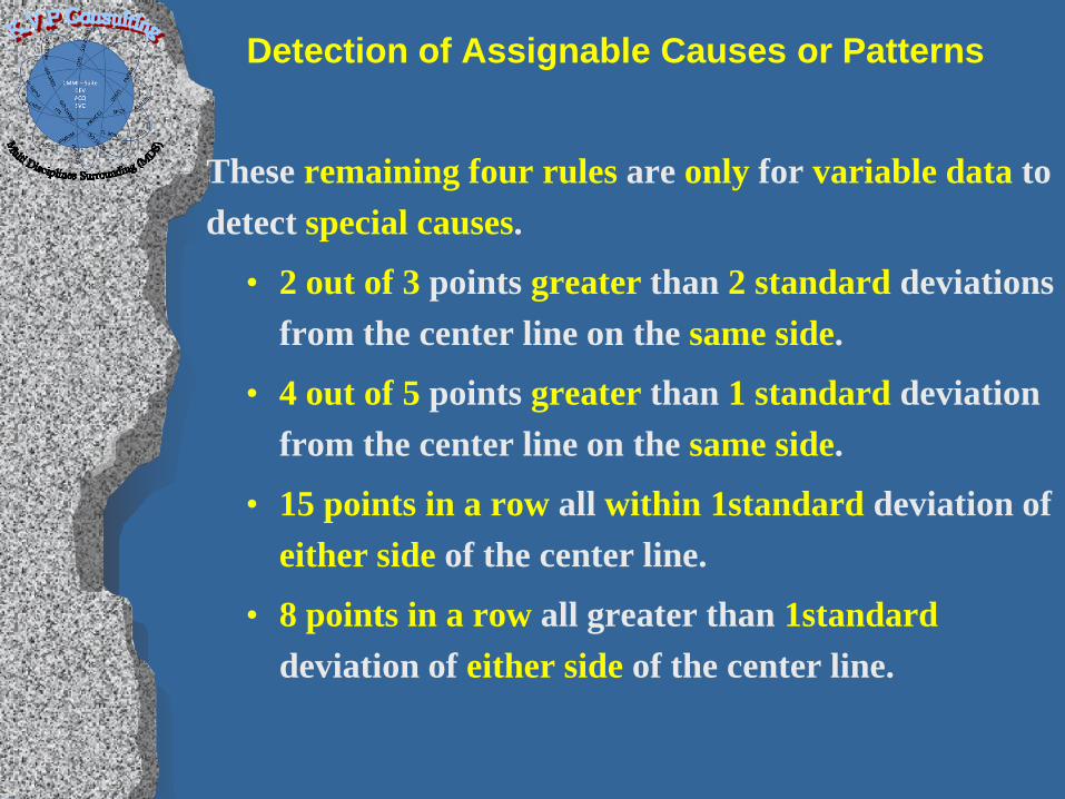
Detection of Assignable Causes or Patterns
These remaining four rules are only for variable data to detect special causes.
• 2 out of 3 points greater than 2 standard deviations from the center line on the same side.
• 4 out of 5 points greater than 1 standard deviation from the center line on the same side.
• 15 points in a row all within 1standard deviation of either side of the center line.
• 8 points in a row all greater than 1standard deviation of either side of the center line.
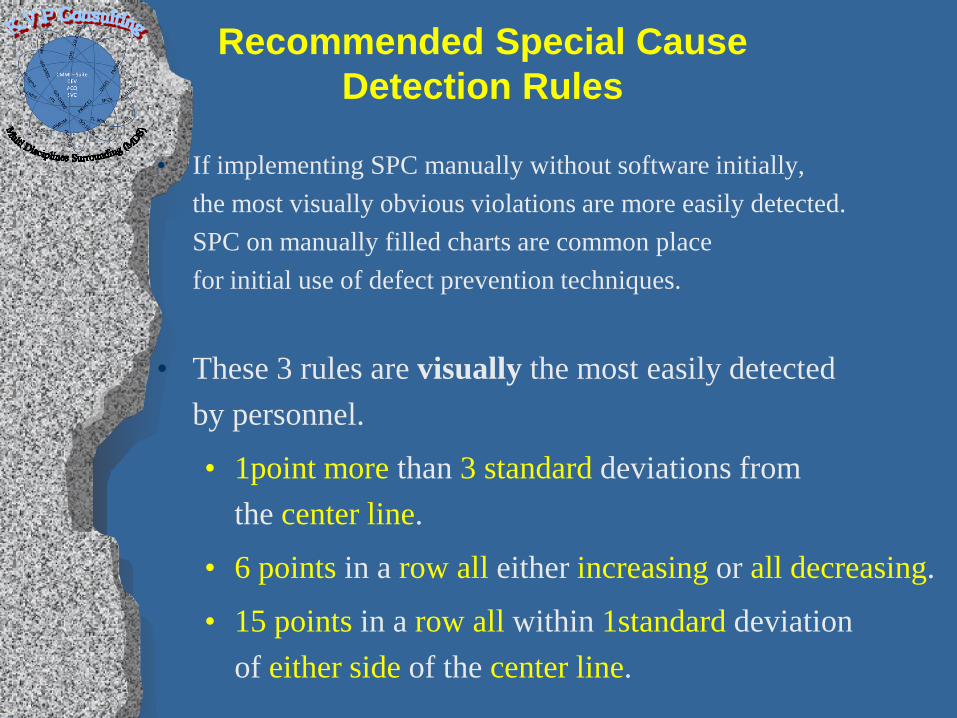
Recommended Special Cause Detection Rules
• If implementing SPC manually without software initially, the most visually obvious violations are more easily detected. SPC on manually filled charts are common place for initial use of defect prevention techniques.
• These 3 rules are visually the most easily detected by personnel.
• 1point more than 3 standard deviations from the center line.
• 6 points in a row all either increasing or all decreasing.
• 15 points in a row all within 1standard deviation of either side of the center line.
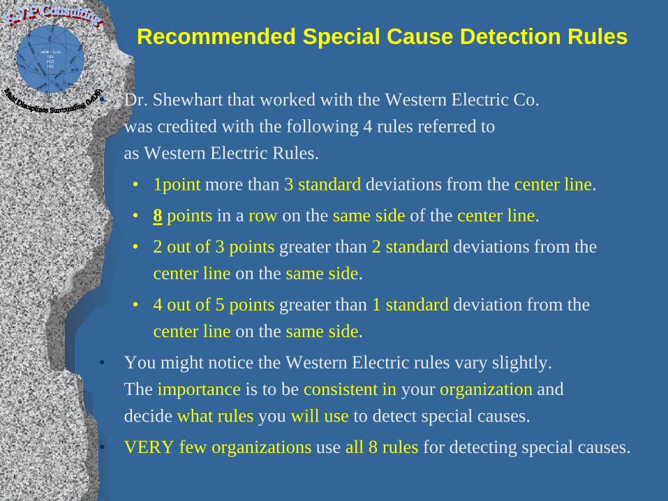
Recommended Special Cause Detection Rules
• Dr. Shewhart that worked with the Western Electric Co. was credited with the following 4 rules referred to as Western Electric Rules.
• 1point more than 3 standard deviations from the center line.
• 8 points in a row on the same side of the center line.
• 2 out of 3 points greater than 2 standard deviations from the center line on the same side.
• 4 out of 5 points greater than 1 standard deviation from the center line on the same side.
• You might notice the Western Electric rules vary slightly. The importance is to be consistent in your organization and decide what rules you will use to detect special causes.
• VERY few organizations use all 8 rules for detecting special causes.
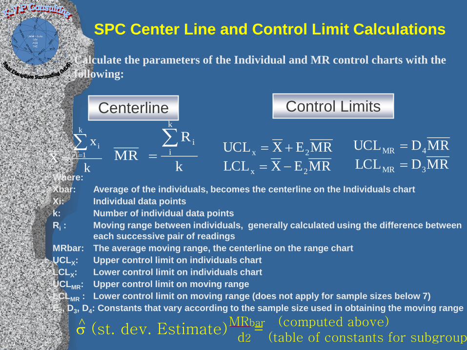
SPC Center Line and Control Limit Calculations
Calculate the parameters of the Individual and MR control charts with the following:
Where: Xbar: Average of the individuals, becomes the centerline on the Individuals chart Xi: Individual data points k: Number of individual data points Ri : Moving range between individuals, generally calculated using the difference between each successive pair of readings MRbar: The average moving range, the centerline on the range chart UCLX: Upper control limit on individuals chart LCLX: Lower control limit on individuals chart UCLMR: Upper control limit on moving range LCLMR : Lower control limit on moving range (does not apply for sample sizes below 7) E2, D3, D4: Constants that vary according to the sample size used in obtaining the moving range
k
xX
k
1ii∑
== k
RRM
k
ii∑
= RMEXUCL 2x +=RMEXLCL 2x −=
RMDUCL 4MR =RMDLCL 3MR =
Centerline Control Limits
MRbar (computed above) d2 (table of constants for subgroup
σ (st. dev. Estimate) =
SPC Center Line and Control Limit Calculations
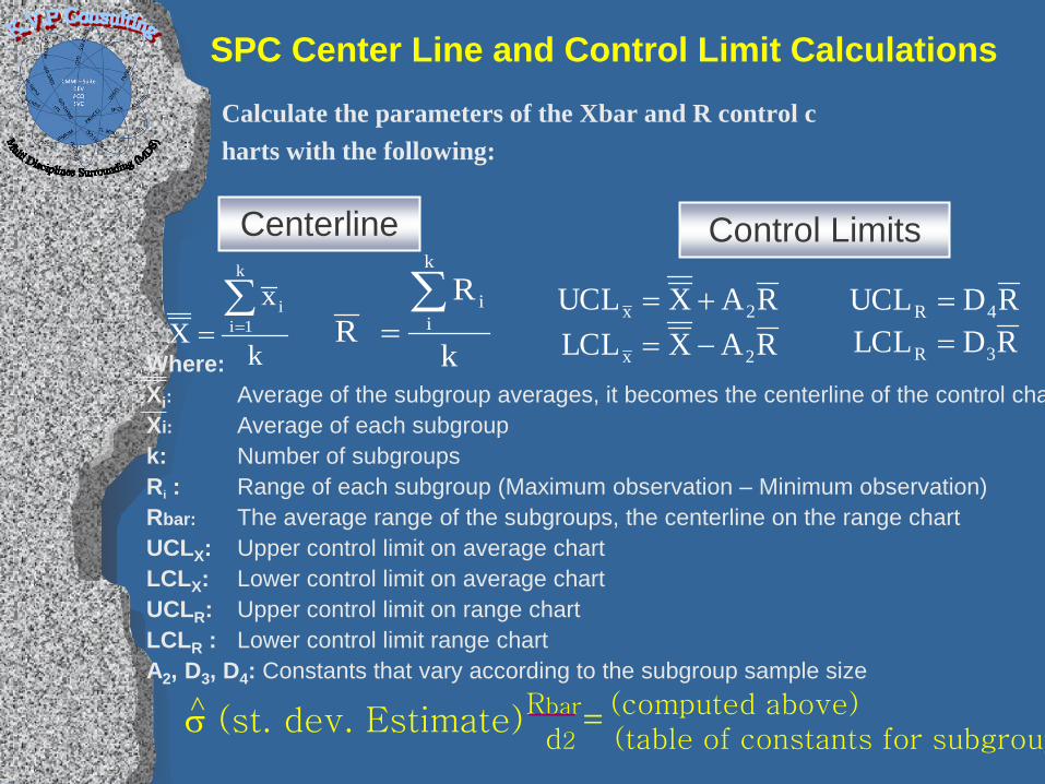
Calculate the parameters of the Xbar and R control c harts with the following:
k
xX
k
1ii∑
==k
RR
k
ii∑
=RAXUCL 2x +=RAXLCL 2x −=
RDUCL 4R =RDLCL 3R =
Centerline Control Limits
Where: Xi: Average of the subgroup averages, it becomes the centerline of the control chaXi: Average of each subgroup k: Number of subgroups Ri : Range of each subgroup (Maximum observation – Minimum observation) Rbar: The average range of the subgroups, the centerline on the range chart UCLX: Upper control limit on average chart LCLX: Lower control limit on average chart UCLR: Upper control limit on range chart LCLR : Lower control limit range chart A2, D3, D4: Constants that vary according to the subgroup sample size
Rbar (computed above) d2 (table of constants for subgroup
σ (st. dev. Estimate) =
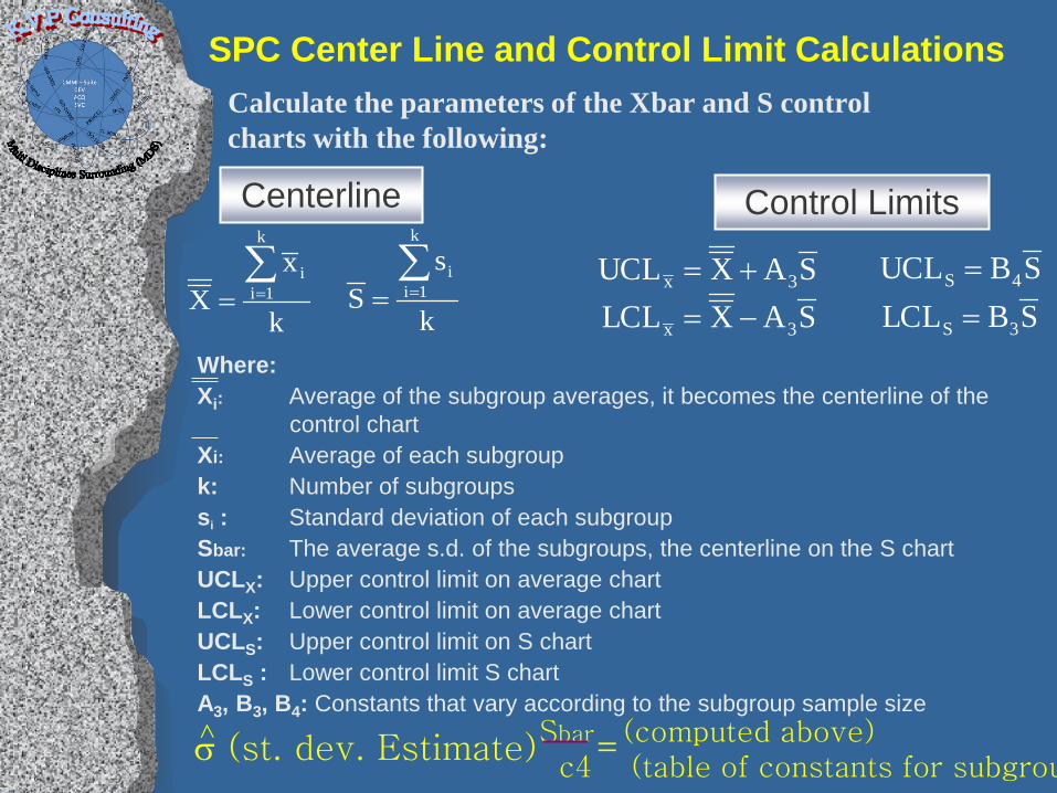
SPC Center Line and Control Limit Calculations Calculate the parameters of the Xbar and S control charts with the following:
Where: Xi: Average of the subgroup averages, it becomes the centerline of the control chart Xi: Average of each subgroup k: Number of subgroups si : Standard deviation of each subgroup Sbar: The average s.d. of the subgroups, the centerline on the S chart UCLX: Upper control limit on average chart LCLX: Lower control limit on average chart UCLS: Upper control limit on S chart LCLS : Lower control limit S chart A3, B3, B4: Constants that vary according to the subgroup sample size
k
xX
k
1ii∑
==SAXUCL 3x +=
Centerline Control Limits
SAXLCL 3x −=k
sS
k
1ii∑
==SBUCL 4S =SBLCL 3S =
Sbar (computed above) c4 (table of constants for subgrou
σ (st. dev. Estimate) =
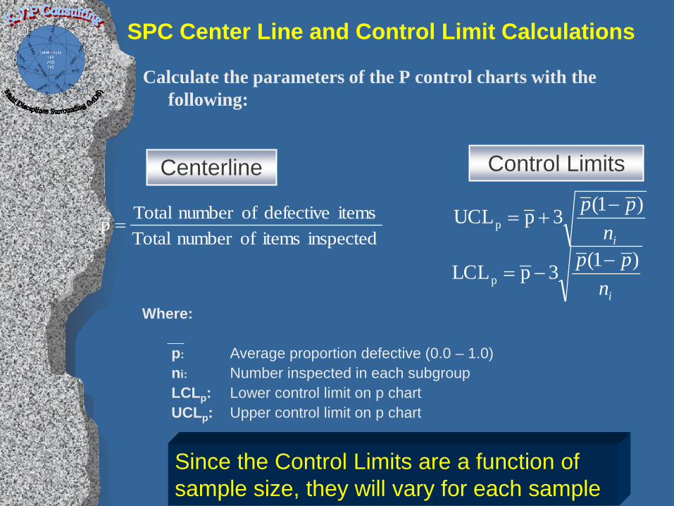
SPC Center Line and Control Limit Calculations
Calculate the parameters of the P control charts with the following:
Where: p: Average proportion defective (0.0 – 1.0) ni: Number inspected in each subgroup LCLp: Lower control limit on p chart UCLp: Upper control limit on p chart
inspected items ofnumber Totalitems defective ofnumber Totalp =
inpp )1(3pUCLp
−+=
Centerline Control Limits
inpp )1(3pLCLp
−−=
Since the Control Limits are a function of sample size, they will vary for each sample
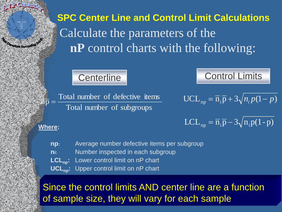
SPC Center Line and Control Limit Calculations Calculate the parameters of the
nP control charts with the following:
Where: np: Average number defective items per subgroup ni: Number inspected in each subgroup LCLnp: Lower control limit on nP chart UCLnp: Upper control limit on nP chart
subgroups ofnumber Totalitems defective ofnumber Totalpn = )1(3pnUCL inp ppni −+=
Centerline Control Limits
p)-p(1n3pnLCL iinp −=
Since the control limits AND center line are a function of sample size, they will vary for each sample
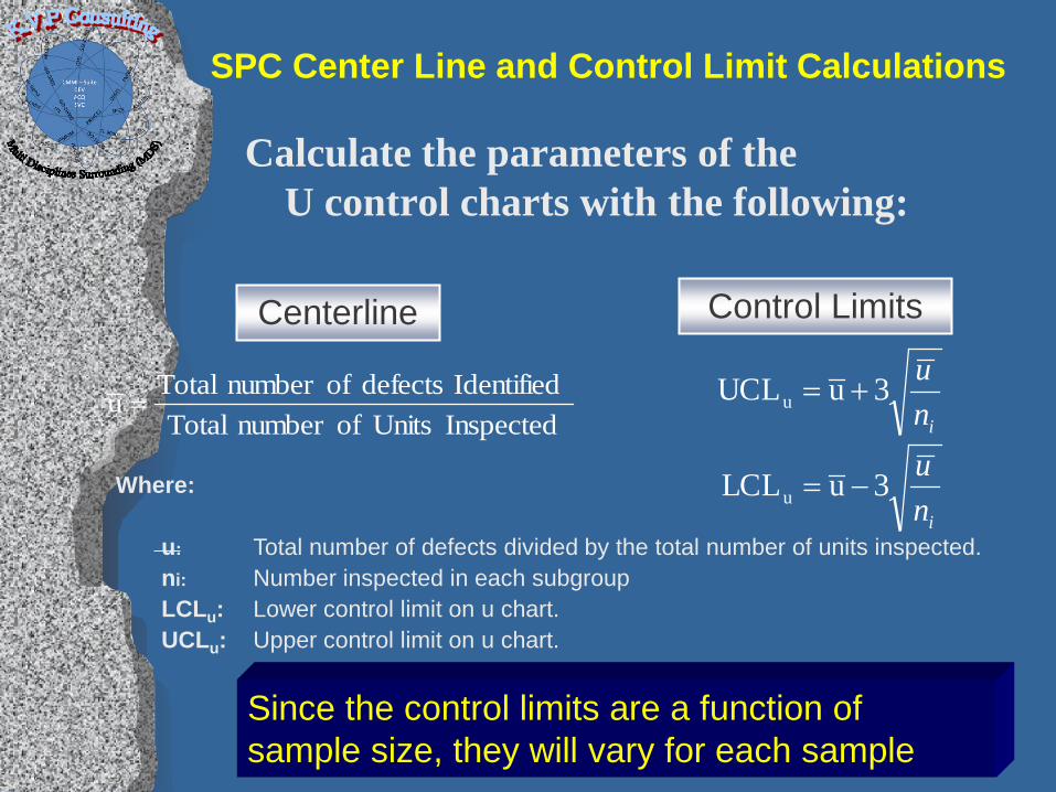
SPC Center Line and Control Limit Calculations
Calculate the parameters of the U control charts with the following:
Where: u: Total number of defects divided by the total number of units inspected. ni: Number inspected in each subgroup LCLu: Lower control limit on u chart. UCLu: Upper control limit on u chart.
Inspected Unitsofnumber TotalIdentified defects ofnumber Totalu =
inu3uUCLu +=
Centerline Control Limits
Since the control limits are a function of sample size, they will vary for each sample
inu3uLCLu −=
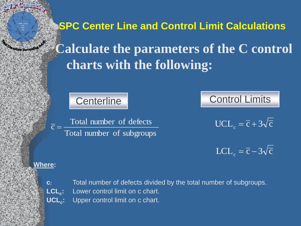
SPC Center Line and Control Limit Calculations
Calculate the parameters of the C control charts with the following:
Where: c: Total number of defects divided by the total number of subgroups. LCLc: Lower control limit on c chart. UCLc: Upper control limit on c chart.
subgroups ofnumber Totaldefects ofnumber Totalc = c3cUCLc +=
Centerline Control Limits
c3cLCLc −=
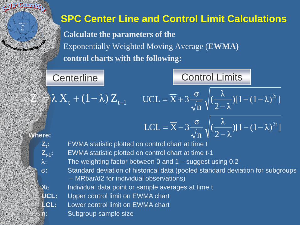
SPC Center Line and Control Limit Calculations Calculate the parameters of the Exponentially Weighted Moving Average (EWMA) control charts with the following:
Where: Zt: EWMA statistic plotted on control chart at time t Zt-1: EWMA statistic plotted on control chart at time t-1 λ: The weighting factor between 0 and 1 – suggest using 0.2 σ: Standard deviation of historical data (pooled standard deviation for subgroups – MRbar/d2 for individual observations) Xt: Individual data point or sample averages at time t UCL: Upper control limit on EWMA chart LCL: Lower control limit on EWMA chart n: Subgroup sample size
1ttt Zλ)(1 X λZ −−+= ]λ)(1)[1λ2
λ(nσ3XUCL 2t−−
−+=
Centerline Control Limits
]λ)(1)[1λ2
λ(nσ3XLCL 2t−−
−−=

UNDERSTANDING VARIATION
Sources of Variation • Variation exists in all processes. • Variation can be categorized as either:
• Common or Random causes of variation, or • Random causes that we cannot identify • Unavoidable, e.g. slight differences in process
variables like diameter, weight, service time, temperature
• Assignable causes of variation • Causes can be identified and eliminated: poor
employee training, worn tool, machine needing repair
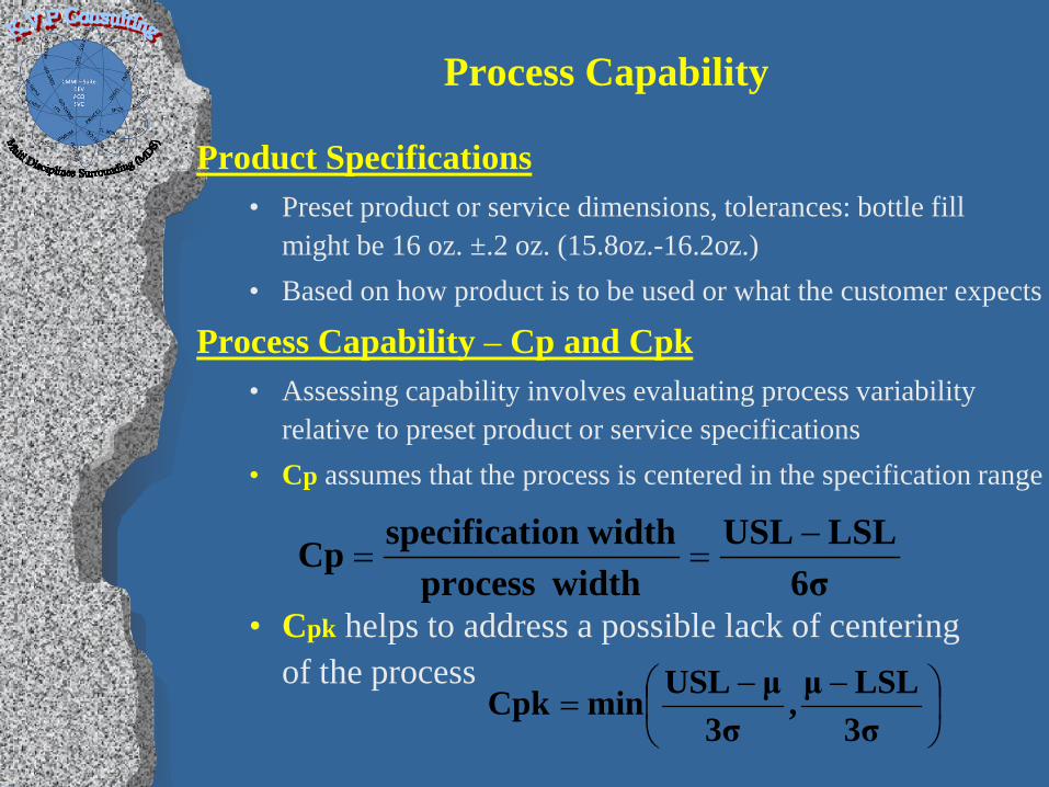
Process Capability
Product Specifications • Preset product or service dimensions, tolerances: bottle fill
might be 16 oz. ±.2 oz. (15.8oz.-16.2oz.) • Based on how product is to be used or what the customer expects
Process Capability – Cp and Cpk • Assessing capability involves evaluating process variability
relative to preset product or service specifications • Cp assumes that the process is centered in the specification range
• Cpk helps to address a possible lack of centering
of the process
6σLSLUSL
width processwidth ionspecificatCp −
==
−−
=3σLSLμ,
3σμUSLminCpk
Relationship between Process Variability and
Specification Width
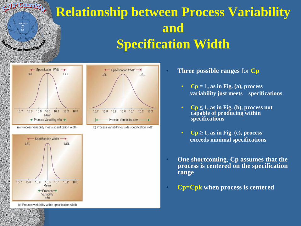
• Three possible ranges for Cp
• Cp = 1, as in Fig. (a), process variability just meets specifications • Cp ≤ 1, as in Fig. (b), process not
capable of producing within specifications
• Cp ≥ 1, as in Fig. (c), process exceeds minimal specifications
• One shortcoming, Cp assumes that the process is centered on the specification range
• Cp=Cpk when process is centered
Measures of Variation
Measures of Variation include:
•The range
•The Variance
•The Standard Deviation
•The Mean Absolute Deviation
The standard deviation is just the square root of the variance
Measures of Variation
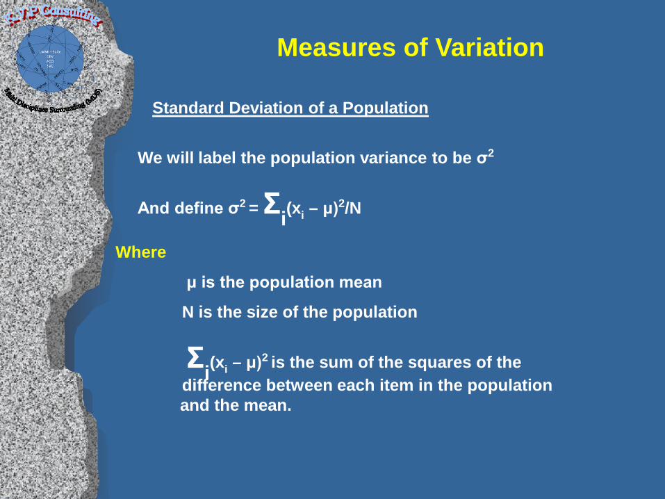
Standard Deviation of a Population
We will label the population variance to be σ2
And define σ2 = Σi(xi – μ)2/N
Where
μ is the population mean
N is the size of the population
Σi(xi – μ)2 is the sum of the squares of the difference between each item in the population and the mean.
Measures of Variation Suppose a student receives the following quiz grades:
{82, 68, 74, 86, 90, 88, 62, 75, 80, 55}
For this student, these grades are the total population of her scores that are used to calculate her mean or average grade. We obtain:
μ = (82 + 68 + 74 + 86 + 90 + 88 + 62 + 75 + 80 + 55)/10
= 760/10 = 76
The mean of this population is 76
Measures of Variation
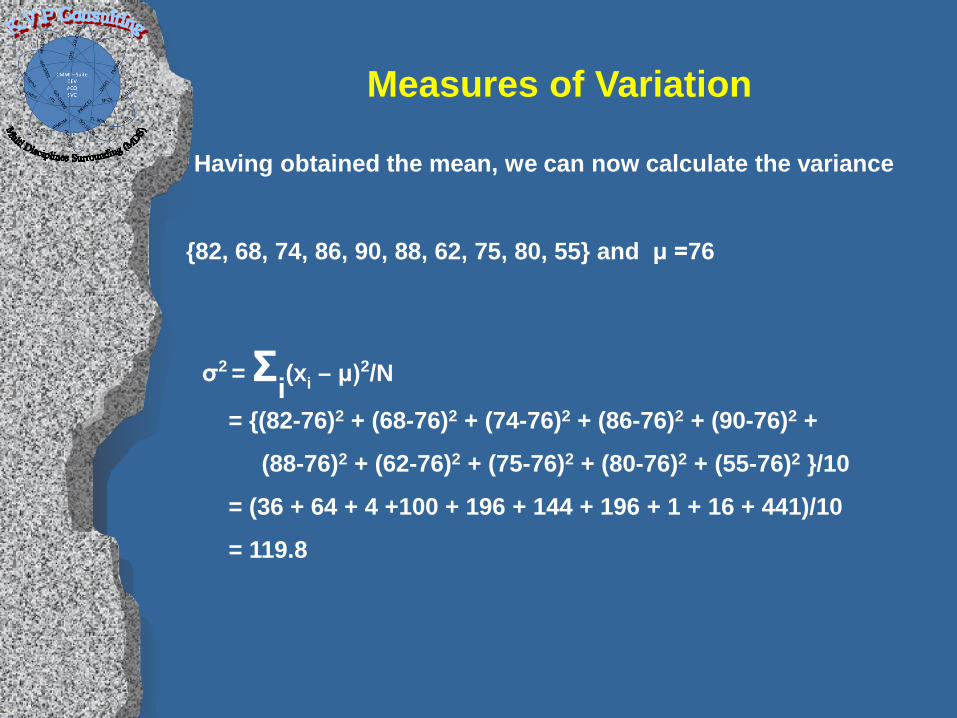
Having obtained the mean, we can now calculate the variance
σ2 = Σi(xi – μ)2/N
= {(82-76)2 + (68-76)2 + (74-76)2 + (86-76)2 + (90-76)2 +
(88-76)2 + (62-76)2 + (75-76)2 + (80-76)2 + (55-76)2 }/10
= (36 + 64 + 4 +100 + 196 + 144 + 196 + 1 + 16 + 441)/10
= 119.8
{82, 68, 74, 86, 90, 88, 62, 75, 80, 55} and μ =76
Measures of Variation
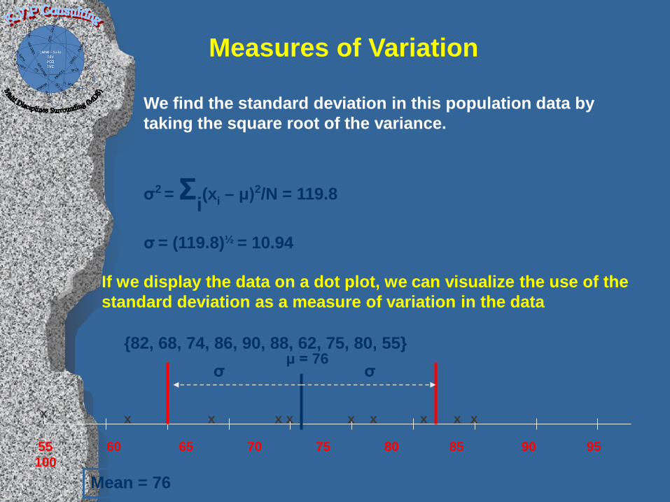
We find the standard deviation in this population data by taking the square root of the variance.
σ2 = Σi(xi – μ)2/N = 119.8
σ = (119.8)½ = 10.94
If we display the data on a dot plot, we can visualize the use of the standard deviation as a measure of variation in the data
55 60 65 70 75 80 85 90 95 100
x x x x x x x x x x
Mean = 76
μ = 76 σ σ
{82, 68, 74, 86, 90, 88, 62, 75, 80, 55}
Measures of Variation
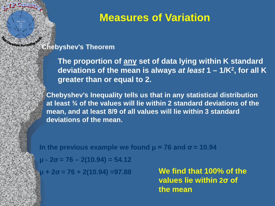
Chebyshev’s Theorem
The proportion of any set of data lying within K standard deviations of the mean is always at least 1 – 1/K2, for all K greater than or equal to 2.
Chebyshev’s Inequality tells us that in any statistical distribution at least ¾ of the values will lie within 2 standard deviations of the mean, and at least 8/9 of all values will lie within 3 standard deviations of the mean.
In the previous example we found μ = 76 and σ = 10.94
μ - 2σ = 76 – 2(10.94) = 54.12
μ + 2σ = 76 + 2(10.94) =97.88 We find that 100% of the values lie within 2σ of the mean

CASE STUDY – FIRST PHASE
REDUCING VARIATION
Selecting improvements to implement
• High-level objective evaluation of all potential improvements • Impact of each improvement • Cost to implement each improvement • Time to implement each improvement
• Balance desire with quantifiable evaluation • Engineering always wants the gold standard • Sales always wants inventory • Production always wants more capacity
Impact of the improvement
• Time frame of improvements • Long-term vs. Short-term effectiveness
• If a supplier will lose a major customer because of defects, the short term benefit will prevail first.
• Effectiveness of the improvement types • Removing the root cause of the defect • Monitoring/flagging for the condition that produces a
defect • Inspecting to determine if the defect occurred • Training people not to produce defects
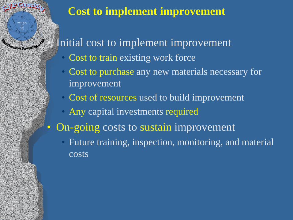
Cost to implement improvement
• Initial cost to implement improvement • Cost to train existing work force • Cost to purchase any new materials necessary for
improvement • Cost of resources used to build improvement • Any capital investments required
• On-going costs to sustain improvement • Future training, inspection, monitoring, and material
costs
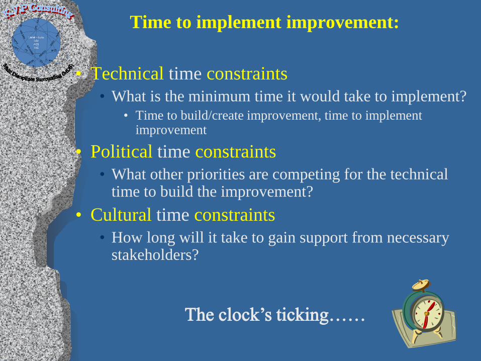
Time to implement improvement:
• Technical time constraints • What is the minimum time it would take to implement?
• Time to build/create improvement, time to implement improvement
• Political time constraints • What other priorities are competing for the technical
time to build the improvement? • Cultural time constraints
• How long will it take to gain support from necessary stakeholders?
The clock’s ticking……
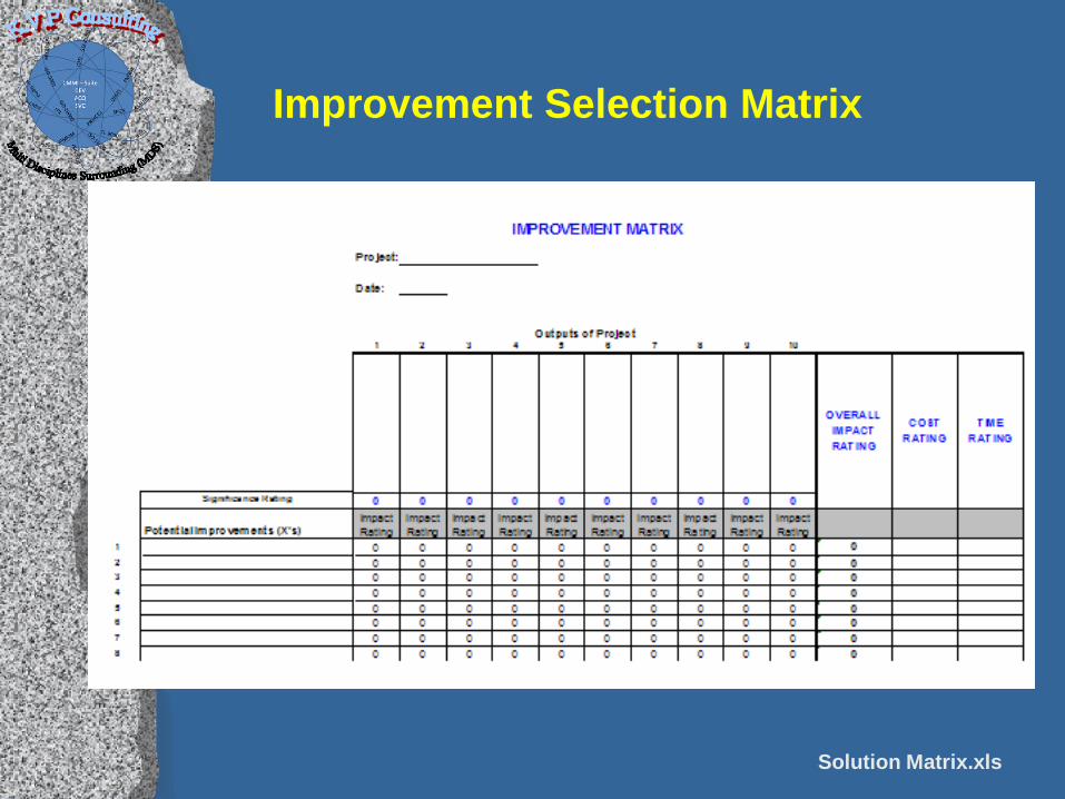
Improvement Selection Matrix
Solution Matrix.xls
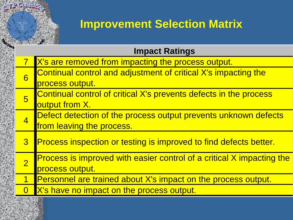
Improvement Selection Matrix
Impact Ratings7 X's are removed from impacting the process output.
6 Continual control and adjustment of critical X's impacting the process output.
5 Continual control of critical X's prevents defects in the process output from X.
4 Defect detection of the process output prevents unknown defects from leaving the process.
3 Process inspection or testing is improved to find defects better.
2 Process is improved with easier control of a critical X impacting the process output.
1 Personnel are trained about X's impact on the process output.0 X's have no impact on the process output.
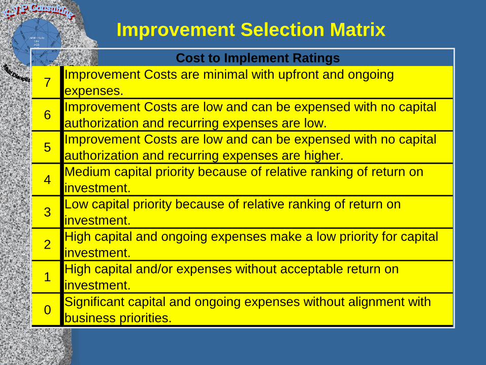
Improvement Selection Matrix Cost to Implement Ratings
7 Improvement Costs are minimal with upfront and ongoing expenses.
6 Improvement Costs are low and can be expensed with no capital authorization and recurring expenses are low.
5 Improvement Costs are low and can be expensed with no capital authorization and recurring expenses are higher.
4 Medium capital priority because of relative ranking of return on investment.
3 Low capital priority because of relative ranking of return on investment.
2 High capital and ongoing expenses make a low priority for capital investment.
1 High capital and/or expenses without acceptable return on investment.
0 Significant capital and ongoing expenses without alignment with business priorities.
Improvement Selection Matrix
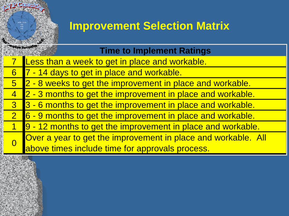
Time to Implement Ratings7 Less than a week to get in place and workable.6 7 - 14 days to get in place and workable.5 2 - 8 weeks to get the improvement in place and workable.4 2 - 3 months to get the improvement in place and workable.3 3 - 6 months to get the improvement in place and workable.2 6 - 9 months to get the improvement in place and workable.1 9 - 12 months to get the improvement in place and workable.
0 Over a year to get the improvement in place and workable. All above times include time for approvals process.

Example of Completed Solution Selection Matrix
86 7 7 421452 7 7 254863 3 6 113436 5 5 90060 3 3 54063 5 2 630
OVERALL IMPACT RATING
COST RATING
TIME RATING
OVERALL RATING
Out
side
noi
ses
do n
ot
inte
rfer
with
spe
aker
s
Cof
fee
is h
ot a
nd ri
ch
tast
ing
Plen
ty o
f bot
tled
wat
er
avai
labl
e
Food
cho
ices
incl
ude
"hea
lthy
choi
ces"
Significance Rating 10 9 8 9
Potential ImprovementsImpact Rating
Impact Rating
Impact Rating
Impact Rating
1 Hotel staff monitors room 2 2 6 02 Mgmt visits/leaves ph # 2 0 4 03 Replace old coffee makers/coffee 0 7 0 04 Menus provided with nutrition info 0 0 0 45 Comp. gen. "quiet time" scheduled 6 0 0 06 Dietician approves menus 0 0 0 7
Improvement Selection Matrix Output
Improvements with the higher overall rating should be given first priority. Keep in mind that long time frame capital investments, etc. should have parallel efforts to keep delays from further occurring.
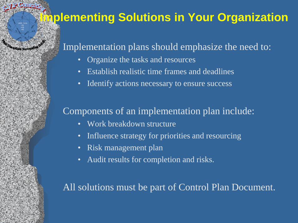
Implementing Solutions in Your Organization
Implementation plans should emphasize the need to: • Organize the tasks and resources • Establish realistic time frames and deadlines • Identify actions necessary to ensure success
Components of an implementation plan include:
• Work breakdown structure • Influence strategy for priorities and resourcing • Risk management plan • Audit results for completion and risks.
All solutions must be part of Control Plan Document.
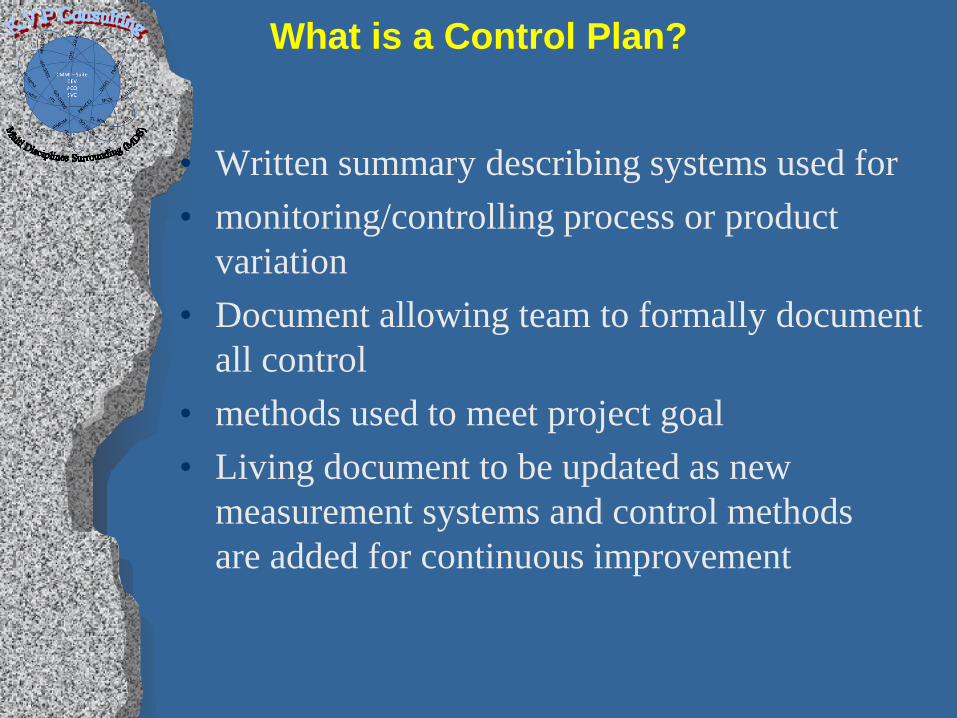
What is a Control Plan?
• Written summary describing systems used for • monitoring/controlling process or product
variation • Document allowing team to formally document
all control • methods used to meet project goal • Living document to be updated as new
measurement systems and control methods are added for continuous improvement
What is a Control Plan?
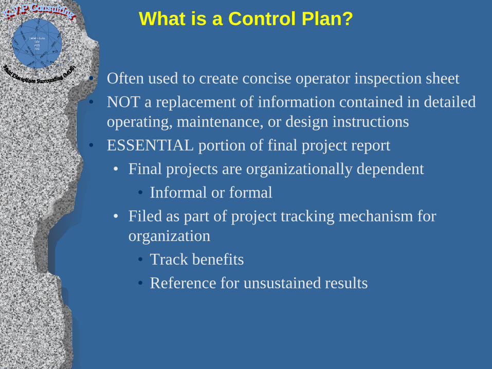
• Often used to create concise operator inspection sheet • NOT a replacement of information contained in detailed
operating, maintenance, or design instructions • ESSENTIAL portion of final project report
• Final projects are organizationally dependent • Informal or formal
• Filed as part of project tracking mechanism for organization
• Track benefits • Reference for unsustained results
WHO Should Create a Control Plan
The team working on the project!!!! ANYONE who has a role in defining, executing or changing the process:
• Associates • Technical Experts • Supervisors • Managers • Site Manager • Human Resources
Why Do We Need a Control Plan?
Project results need to be sustained. • Control Plan requires operators/engineers, managers, etc. to
follow designated control methods to guarantee product quality throughout system
• Allows to move onto other projects! • Prevents need for constant heroes in an organization who
repeatedly solve the same problems • Control Plans are becoming more of a customer requirement
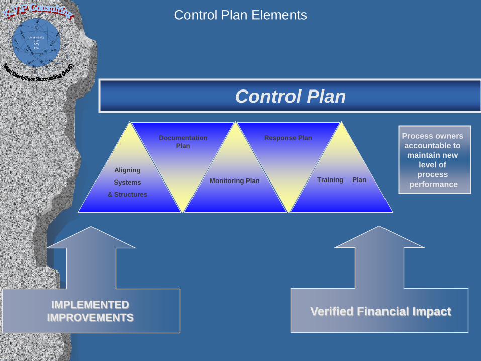
Control Plan Elements
IMPLEMENTED IMPROVEMENTS
Control Plan
Aligning
Systems
& Structures
Documentation Plan
Monitoring Plan
Response Plan
Training Plan
Verified Financial Impact
Process owners accountable to maintain new
level of process
performance
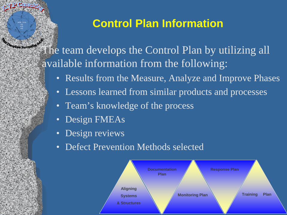
Control Plan Information
The team develops the Control Plan by utilizing all available information from the following:
• Results from the Measure, Analyze and Improve Phases • Lessons learned from similar products and processes • Team’s knowledge of the process • Design FMEAs • Design reviews • Defect Prevention Methods selected
Aligning
Systems
& Structures
Documentation Plan
Monitoring Plan
Response Plan
Training Plan
Training Plan
Who/What organizations require training? • Those impacted by the improvements
• People who are involved in the process impacted by the improvement
• People who support the process impacted by the improvement
• Those impacted by the Control Plan • Process owners/managers • People who support the processes involved in the
Control Plan • People who will make changes to the process in the
future
Training
Plan
Training Plan
Who will complete the training? • Immediate training
• The planning, development and execution is a responsibility of the project team
• Typically some of the training is conducted by the project team
• Qualified trainers • Typically owned by a training department or process owner • Those who are responsible for conducting the on-going training
must be identified
Specific training materials need developing.
• PowerPoint, On the Job checklist, Exercises, etc.
Training
Plan
Training Plan
When will training be conducted? What is the timeline to train everyone on the new
process(es)? What will trigger ongoing training?
• New employee orientation? • Refresher training? • Part of the response plan when monitoring shows
performance degrading?
Training
Plan
Documentation Plan
Documentation is necessary to ensure that what has been learned from the project is shared and institutionalized:
• Used to aid implementation of solutions • Used for on-going training
This is often the actual Final Report some organizations use.
Documentation must be kept current to be useful
Documentation Plan
Documentation Plan
Items to be included in the documentation plan: • Process documentation
• Updated Process maps/flowcharts • Procedures (SOP’s) • FMEA
• Control Plan documentation • Training manuals • Monitoring plan—process management charts, reports, sops • Response plan—FMEA • Systems and structures—job descriptions, performance management
objectives
Documentation Plan
Documentation Plan
Assigning responsibility for documentation plan: • Responsibility at implementation
• Black belt ensures all documents are current at hand off • Black belt ensures there is a process to modify
documentation as the process changes in place • Black belt ensures there is a process in place to review
documentation on regular basis for currency/accuracy • Responsibility for ongoing process (organizationally based)
• Plan must outline who is responsible for making updates/modifications to documentation as they occur
• Plan must outline who is responsible to review documents—ensuring currency/accuracy of documentation
Documentation Plan
Documentation Plan
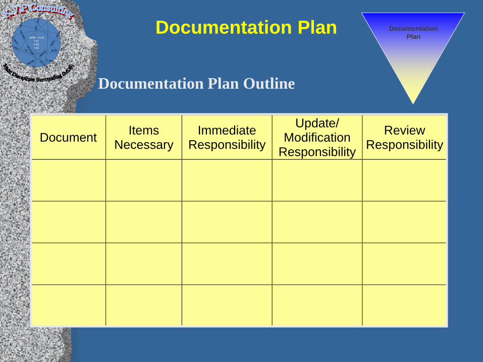
Documentation Plan Outline
Documentation Plan
Document ItemsNecessary
ImmediateResponsibility
Update/Modification
Responsibility
ReviewResponsibility
Monitoring Plan
Monitoring Plan
Purpose of a monitoring plan: • Assures gains are achieved and sustained • Provides insight for future process improvement
activities Development of a monitoring plan:
• Belt is responsible for the development of the monitoring plan
• Team members will help to develop the plan • Stakeholders must be consulted • Organizations with financial tracking would monitor
results.
Monitoring Plan
Monitoring Plan
Sustaining the monitoring plan: • Functional managers will be responsible for
adherence to the monitoring plan • They must be trained on how to do this • They must be made accountable for adherence
Monitoring Plan
Tests: • When to Sample
• After training • Regular intervals • Random intervals (often in auditing sense)
• How to Sample • How to Measure
Monitoring Plan
Monitoring Plan
Statistical process control: • Control charts
• Posted in area where data collected • Plot data points real time
• Act on Out of Control Response with guidelines from the Out of Control Action Plan (OCAP).
• Record actions taken to achieve in-control results.
• Notes impacting performance on chart should be encouraged
• Establishing new limits • Based on signals that process performance has changed
Monitoring Plan
Response Plan
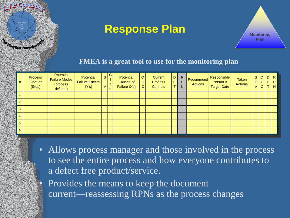
FMEA is a great tool to use for the monitoring plan
• Allows process manager and those involved in the process to see the entire process and how everyone contributes to a defect free product/service.
• Provides the means to keep the document current—reassessing RPNs as the process changes
#Process Function
(Step)
Potential Failure Modes
(process defects)
Potential Failure Effects
(Y's)
SEV
Clas
Potential Causes of
Failure (X's)
OCC
Current Process Controls
DET
RPN
Recommend Actions
Responsible Person &
Target Date
Taken Actions
SEV
OCC
DET
RPN
1
2
3
4
5
6
Monitoring Plan
Monitoring Plan
Check Lists/Matrices • Key items to check • Decision criteria; decision road map • Multi-variable tables
Visual Management
• Alerts or signals to trigger action. • Empty bins being returned to when need stock replenished • Red/yellow/green reports to signal process performance
• Can be audible also.
Monitoring Plan
Response Plan
Response plans—outline process(es) to follow when there is a defect or Out of Control from monitoring:
• Out of control point on control chart • Non random behavior within control limits in
control chart • Condition/variable proven to produce defects present in
process • Check sheet failure • Automation failure
Response to poor process results are a must in training.
Response plans are living documents updated with new information as it becomes available
Response Plan
Response Plan
Components of response plan:
• The triggers for a response • What are the failure modes to check for? • Usually monitor the highest risk x's in the process
• The recommended response for the failure mode • The responsibilities for responding to the failure
mode • Documentation of response plan being followed in
a failure mode • Detailed information on the conditions
surrounding the failure mode
Response Plan
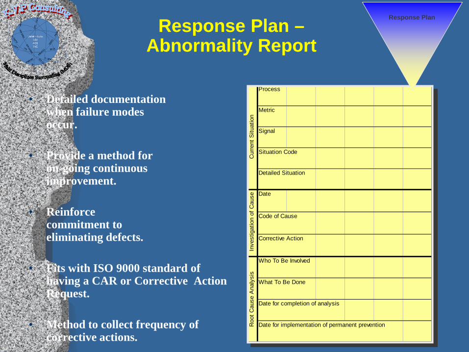
Response Plan – Abnormality Report
• Detailed documentation when failure modes occur.
• Provide a method for on-going continuous improvement.
• Reinforce
commitment to eliminating defects.
• Fits with ISO 9000 standard of having a CAR or Corrective Action Request.
• Method to collect frequency of corrective actions.
Process
Metric
Signal
Situation Code
Detailed Situation
Date
Code of Cause
Corrective Action
Who To Be Involved
What To Be Done
Date for completion of analysis
Date for implementation of permanent prevention
Cur
rent
Situ
atio
nIn
vest
igat
ion
of C
ause
Roo
t Cau
se A
naly
sis
Response Plan
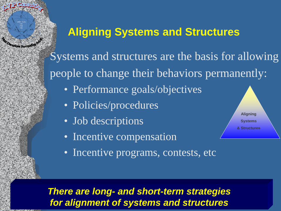
Aligning Systems and Structures
Systems and structures are the basis for allowing people to change their behaviors permanently:
• Performance goals/objectives • Policies/procedures • Job descriptions • Incentive compensation • Incentive programs, contests, etc
There are long- and short-term strategies for alignment of systems and structures
Aligning
Systems
& Structures
Aligning Systems and Structures
• Get rid of measurements that do not align with desired behaviors
• Get rid of multiple measures for the same desired behaviors
• Implement measures that align with desired behaviors currently not motivated by incentives
• Change management must consider your process changes and how the process will respond?
• Are the hourly incentives hurting your chance of success?
Aligning
Systems
& Structures
Project Sign Off
Best method to assure acceptance of Control Plan is having supervisors and management for the area involved.
• Meeting for a summary report • Specific changes to the process highlighted • Information where Control Plan is filed
Aligning
Systems
& Structures

CASE STUDY – SECOND PHASE
‘Cheshire Puss,’ she began, … `Would you tell me, please, which way I ought to go from here?’ ‘That depends a good deal on where you want to get to,' said the Cat.
Why to Monitor Processes
’I don't much care where –’ said Alice. ’Then it doesn't matter which way you go,' said the Cat. ‘- so long as I get somewhere,' Alice added as an explanation. ‘Oh, you're sure to do that,' said the Cat, ‘if you only walk long enough.’
Tell me where you want to be and I will show (measure) you the way
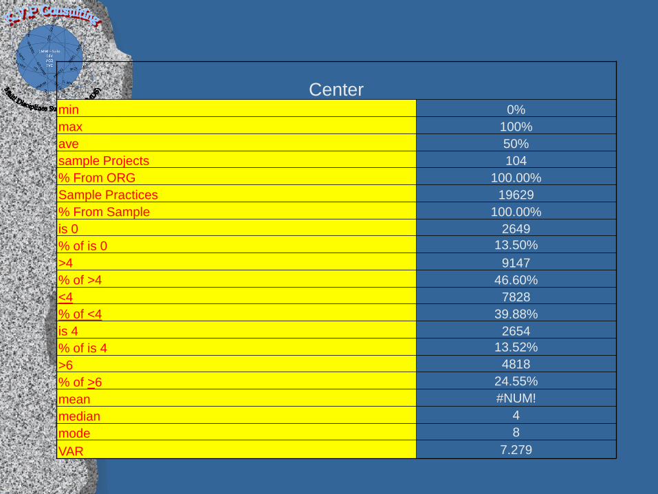
Center
min 0% max 100% ave 50% sample Projects 104 % From ORG 100.00% Sample Practices 19629 % From Sample 100.00% is 0 2649 % of is 0 13.50% >4 9147 % of >4 46.60% <4 7828 % of <4 39.88% is 4 2654 % of is 4 13.52% >6 4818 % of >6 24.55% mean #NUM! median 4 mode 8 VAR 7.279
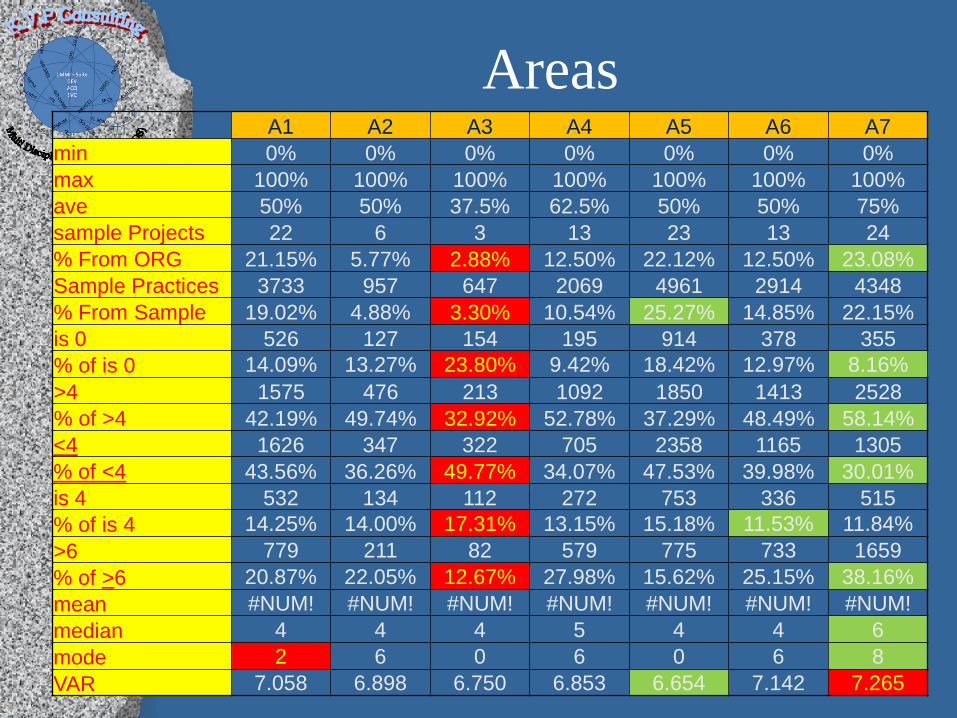
Areas A1 A2 A3 A4 A5 A6 A7 min 0% 0% 0% 0% 0% 0% 0% max 100% 100% 100% 100% 100% 100% 100% ave 50% 50% 37.5% 62.5% 50% 50% 75% sample Projects 22 6 3 13 23 13 24 % From ORG 21.15% 5.77% 2.88% 12.50% 22.12% 12.50% 23.08% Sample Practices 3733 957 647 2069 4961 2914 4348 % From Sample 19.02% 4.88% 3.30% 10.54% 25.27% 14.85% 22.15% is 0 526 127 154 195 914 378 355 % of is 0 14.09% 13.27% 23.80% 9.42% 18.42% 12.97% 8.16% >4 1575 476 213 1092 1850 1413 2528 % of >4 42.19% 49.74% 32.92% 52.78% 37.29% 48.49% 58.14% <4 1626 347 322 705 2358 1165 1305 % of <4 43.56% 36.26% 49.77% 34.07% 47.53% 39.98% 30.01% is 4 532 134 112 272 753 336 515 % of is 4 14.25% 14.00% 17.31% 13.15% 15.18% 11.53% 11.84% >6 779 211 82 579 775 733 1659 % of >6 20.87% 22.05% 12.67% 27.98% 15.62% 25.15% 38.16% mean #NUM! #NUM! #NUM! #NUM! #NUM! #NUM! #NUM! median 4 4 4 5 4 4 6 mode 2 6 0 6 0 6 8 VAR 7.058 6.898 6.750 6.853 6.654 7.142 7.265
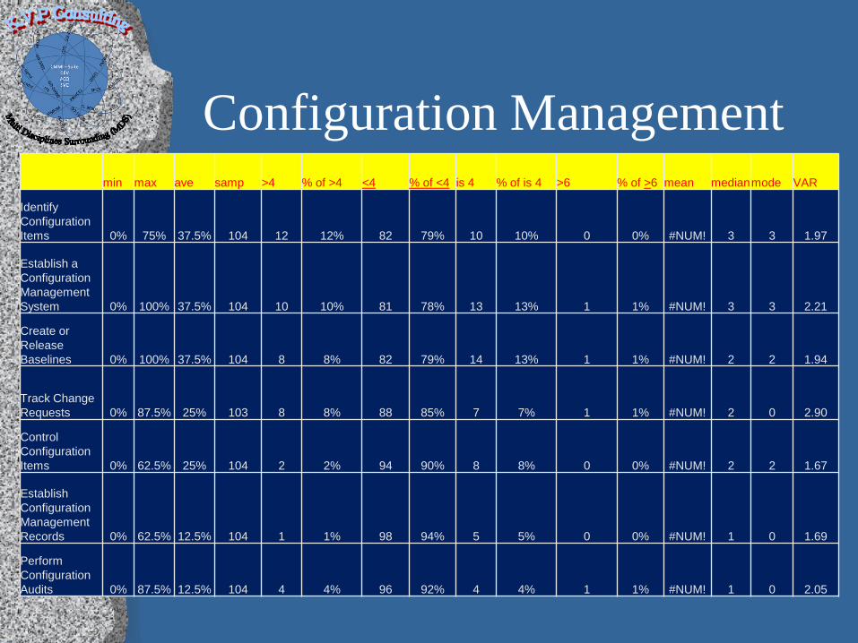
Configuration Management min max ave samp >4 % of >4 <4 % of <4 is 4 % of is 4 >6 % of >6 mean median mode VAR
Identify Configuration Items 0% 75% 37.5% 104 12 12% 82 79% 10 10% 0 0% #NUM! 3 3 1.97
Establish a Configuration Management System
0% 100% 37.5% 104 10 10% 81 78% 13 13% 1 1% #NUM! 3 3 2.21
Create or Release Baselines 0% 100% 37.5% 104 8 8% 82 79% 14 13% 1 1% #NUM! 2 2 1.94
Track Change Requests 0% 87.5% 25% 103 8 8% 88 85% 7 7% 1 1% #NUM! 2 0 2.90
Control Configuration Items 0% 62.5%
25% 104 2 2% 94 90% 8 8% 0 0% #NUM! 2 2 1.67
Establish Configuration Management Records 0% 62.5% 12.5% 104 1 1% 98 94% 5 5% 0 0% #NUM! 1 0 1.69
Perform Configuration Audits 0% 87.5% 12.5% 104 4 4% 96 92% 4 4% 1 1% #NUM! 1 0 2.05
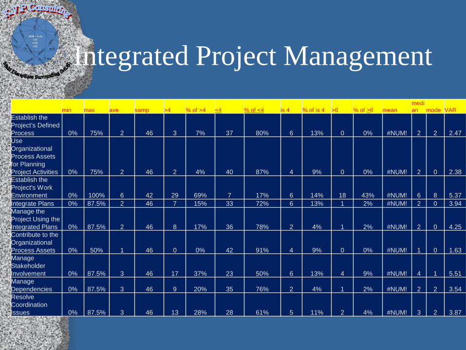
Integrated Project Management
min max ave samp >4 % of >4 <4 % of <4 is 4 % of is 4 >6 % of >6 mean median mode VAR
Establish the Project’s Defined Process 0% 75% 2 46 3 7% 37 80% 6 13% 0 0% #NUM! 2 2 2.47 Use Organizational Process Assets for Planning Project Activities 0% 75% 2 46 2 4% 40 87% 4 9% 0 0% #NUM! 2 0 2.38 Establish the Project's Work Environment 0% 100% 6 42 29 69% 7 17% 6 14% 18 43% #NUM! 6 8 5.37 Integrate Plans 0% 87.5% 2 46 7 15% 33 72% 6 13% 1 2% #NUM! 2 0 3.94 Manage the Project Using the Integrated Plans 0% 87.5% 2 46 8 17% 36 78% 2 4% 1 2% #NUM! 2 0 4.25 Contribute to the Organizational Process Assets 0% 50% 1 46 0 0% 42 91% 4 9% 0 0% #NUM! 1 0 1.63 Manage Stakeholder Involvement 0% 87.5% 3 46 17 37% 23 50% 6 13% 4 9% #NUM! 4 1 5.51 Manage Dependencies 0% 87.5% 3 46 9 20% 35 76% 2 4% 1 2% #NUM! 2 2 3.54 Resolve Coordination Issues 0% 87.5% 3 46 13 28% 28 61% 5 11% 2 4% #NUM! 3 2 3.87
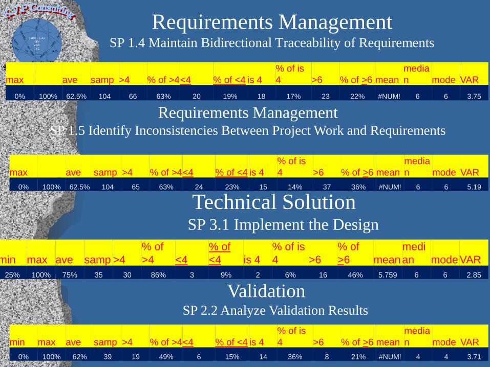
Requirements Management SP 1.4 Maintain Bidirectional Traceability of Requirements
max ave samp >4 % of >4 <4 % of <4 is 4 % of is 4 >6 % of >6 mean
median mode VAR
0% 100% 62.5% 104 66 63% 20 19% 18 17% 23 22% #NUM! 6 6 3.75
Requirements Management SP 1.5 Identify Inconsistencies Between Project Work and Requirements
max ave samp >4 % of >4 <4 % of <4 is 4 % of is 4 >6 % of >6 mean
median mode VAR
0% 100% 62.5% 104 65 63% 24 23% 15 14% 37 36% #NUM! 6 6 5.19
Technical Solution SP 3.1 Implement the Design
min max ave samp >4
% of >4 <4
% of <4 is 4
% of is 4 >6
% of >6 mean
median mode VAR
25% 100% 75% 35 30 86% 3 9% 2 6% 16 46% 5.759 6 6 2.85
Validation SP 2.2 Analyze Validation Results
min max ave samp >4 % of >4 <4 % of <4 is 4 % of is 4 >6 % of >6 mean
median mode VAR
0% 100% 62% 39 19 49% 6 15% 14 36% 8 21% #NUM! 4 4 3.71
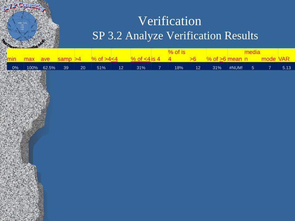
Verification SP 3.2 Analyze Verification Results
min max ave samp >4 % of >4 <4 % of <4 is 4 % of is 4 >6 % of >6 mean
median mode VAR
0% 100% 62.5% 39 20 51% 12 31% 7 18% 12 31% #NUM! 5 7 5.13

Organizational Background and Process ROI
Project Idea and Proposal Preposition Development
• If an average developer day cost is ~7000 • The total Program effort was 10220 day (100%) • The testing phase was 1480 day (14.5%) • Defect that are the result of documentation are 69% of all defects
• If we will assume the to correct 69% of all defects will take around 40% of the
testing duration; means that: • that will be 740 day • With the overall cost of 518000
• However to add 100 review days in the static tests and another 20 of code inspection will end with the cost of 2100000
• And still we have saved at least 3080000 (440 days) • Means that we ware able to reduce 4.5% of the project time

Questions ?
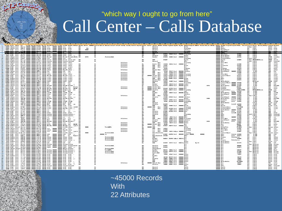
Call Center – Calls Database
~45000 Records With 22 Attributes
“which way I ought to go from here”
~33000 Records With 36 Attributes
Bug Database “which way I ought to go from here”