Electronic copy available at: http://ssrn.com/abstract=2101391

Understanding Peer Effects in Financial Decisions:

Evidence from a Field Experiment∗

Leonardo Bursztyn†

Florian Ederer‡

Bruno Ferman§

Noam Yuchtman¶

August 31, 2012

Abstract

Using a high-stakes field experiment conducted with a financial brokerage, we implement a noveldesign to separately identify two channels of social influence in financial decisions, both widelystudied theoretically. When someone purchases an asset, his peers may also want to purchaseit, both because they learn from his choice (“social learning”) and because his possession of theasset directly affects others’ utility of owning the same asset (“social utility”). We find that bothchannels have statistically and economically significant effects on investment decisions. Theseresults can help shed light on the mechanisms underlying herding behavior in financial markets.

JEL Codes: G00, G11, C93, D03, D14, D83, M31

∗We would like to thank Sushil Bikhchandani, Aislinn Bohren, Arun Chandrasekhar, Shawn Cole, Rui deFigueiredo, Fred Finan, Uri Gneezy, Dean Karlan, Navin Kartik, Larry Katz, Peter Koudijs, Kory Kroft, NicolaLacetera, David Laibson, Edward Leamer, Phil Leslie, Kristof Madarasz, Gustavo Manso, Kris Mitchener, PaulNiehaus, Andrew Oswald, Yona Rubinstein, Ivo Welch, as well as seminar participants at the LSE, Simon Fraser,UCLA, UCLA Anderson, and UCSD Rady for helpful comments and suggestions. Juliana Portella provided excellentresearch assistance. We also thank the Garwood Center for Corporate Innovation, the Russell Sage Foundation andUCLA CIBER for financial support. Finally, we thank the management and staff of the cooperating brokerage firmfor their efforts during the implementation of the study. There was no financial conflict of interest in the implemen-tation of the study; no author was compensated by the partner brokerage or by any other entity for the productionof this article.†UCLA Anderson, bursztyn@ucla.edu.‡UCLA Anderson, florian.ederer@anderson.ucla.edu.§The George Washington School of Business, bferman@gwu.edu.¶UC Berkeley Haas and NBER, yuchtman@haas.berkeley.edu.

Electronic copy available at: http://ssrn.com/abstract=2101391

1 Introduction

People’s choices often look like the choices made by those around them: we wear what is fashionable,

we “have what they’re having,” and we try to “keep up with the Joneses.” Such peer effects have

been analyzed across several fields of economics and social psychology.1 Motivated by concerns

over herding and financial market instability, an especially active area of research has examined

the role of peers in financial decisions. Beyond studying whether peers affect financial decisions,

different channels through which peer effects work have generated their own literatures linking peer

effects to investment decisions, and to financial market instability. Models of herding and asset-

price bubbles, potentially based on very little information, focus on learning from peers’ choices.2

Models in which individuals’ relative income or consumption concerns drive their choice of asset

holdings, and artificially drive up some assets’ prices, focus on peers’ possession of an asset.3 In this

paper, we use a high-stakes field experiment, conducted with a financial brokerage, to separately

identify the causal effects of these channels through which a person’s financial decisions are affected

by his peers’.4

Identifying the causal effect of one’s peers’ behavior on one’s own is notoriously difficult.5

Correlations in the investment or consumption choices of socially-related individuals might arise

1In the economics literature, theoretical models of herding and social learning include Banerjee (1992) andBikhchandani et al. (1992). Becker (1991) studies markets in which a consumer’s demand for a product dependson the aggregate demand for the product. Social influence has also been analyzed under assumptions of boundedrationality, as in DeMarzo et al. (2003) and Guarino and Jehiel (forthcoming). Moscarini et al. (1998) study sociallearning when the state of the world is changing. Calvo-Armengol and Jackson (2010) examine peer pressure as aform of social influence. Empirical work on peer effects has studied a wide range of contexts: the impact of classmatesor friends on education, compensation, and other outcomes (Sacerdote, 2001; Carrell and Hoekstra, 2010; de Giorgi etal., 2010; Duflo et al., 2011; Card and Giuliano, 2011; Shue, 2012); the impact of one’s peers and community on socialindicators and consumption (Bertrand et al., 2000; Kling et al., 2007; Bobonis and Finan, 2009; Dahl et al., 2012;Grinblatt et al., 2008; Kuhn et al., 2011); and, the impact of coworkers on workplace performance (Guryan et al.,2009; Mas and Moretti, 2009; Bandiera et al., 2010). Durlauf (2004) surveys the literature on neighborhood effects.Within the social psychology literature, Asch (1951) studied individuals’ conformity to group norms; Festinger (1954)posited that one resolves uncertainty by learning from others; Burnkrant and Cousineau (1975) distinguished between“informational” and “normative” reasons for conformity.

2See for instance Bikhchandani and Sharma (2000) and Chari and Kehoe (2004). Social learning has also beenstudied experimentally in a laboratory setting by Celen and Kariv (2004).

3Preferences over relative consumption can arise from the (exogenous) presence of other individuals’ consumptiondecisions in one’s utility function, (e.g. Abel, 1990, Gali, 1994, Campbell and Cochrane, 1999) or can arise endoge-nously when one consumes scarce consumption goods, the prices of which depend on the incomes (and consumptionand investment decisions) of other individuals (DeMarzo et al., 2004, DeMarzo et al., 2008).

4See Hirshleifer and Teoh (2003) for a review of models of social learning and herding in financial markets.5An early, thorough discussion of the challenge of identifying causal peer effects is found in Manski (1993).

1

without any causal peer effect: for example, peers select into social groups, and this might generate

correlated choices; peers share common environments (and changes in those environments), and

this, too, might generate correlated choices.6 Equally difficult is identifying why one’s consumption

or investment choices have a social component. Broadly, there are two reasons why a peer’s act of

purchasing an asset (or product, more generally) would affect one’s own choice:

(i) One infers that assets (or products) purchased by others are of higher quality; we refer to

this as social learning.

(ii) One’s utility from possessing an asset (or product) depends directly on the possession of that

asset (or product) by another individual; we call this social utility.

Suppose an investor i considers purchasing a financial asset under uncertainty. In canonical

models of herding based on social learning (e.g., Banerjee, 1992 and Bikhchandani et al., 1992),

information that a peer, investor j, purchased the asset will provide favorable information about the

asset to investor i: investor j would only have purchased the asset if he observed a relatively good

signal of the asset’s return.7 The favorable information conveyed by investor j’s revealed preference

increases the probability that investor i purchases the asset, relative to making a purchase decision

without observing his peer’s decision.8

In our study, we focus on social learning arising only from the information one acquires from

the fact that one’s peer purchased a financial product. We abstract away from the additional

information one might acquire after a peer’s purchase (e.g., by talking to the peer and learning

about the quality of a product) and from any change in behavior due to increased salience of a

product when consumed by one’s peers.9 The impact of learning from a peer’s purchase decision

is the social learning channel.

6A common cultural identity may also affect the decisions made by broad groups of individuals; see Benjamin etal. (2010).

7We assume that investor j here made a choice in isolation, i.e., without peer effects.8Avery and Zemsky (1998) present a model in which information based herds do not occur, due to price adjust-

ments; however, in our setting there is no asset price adjustment (see also Chari and Kehoe, 2004).9The asset sold in our field experiment was designed to make this abstraction possible. This is discussed in detail

in Section 2.1.

2

Typically, investor j’s decision to purchase the asset will also imply that investor j possesses

the asset. If investor j’s possession of the asset directly affects investor i’s utility of owning the

same asset, then observing investor j purchasing the asset (implying investor j’s possession of the

asset) can increase the likelihood that investor i purchases the asset for reasons other than social

learning.

A direct effect of investor j’s possession of a financial asset on investor i’s utility might arise for

a variety of reasons widely discussed in the finance literature. First, investors may be concerned

with their incomes or consumption levels relative to their peers (“keeping up with the Joneses”,

as in Abel, 1990, Gali, 1994, and Campbell and Cochrane, 1999).10 Investors will thus want to

purchase assets possessed by their peers in order to avoid falling behind if the assets’ prices rise.

Even if investors do not directly care about their peers’ income or consumption, they may worry

that increases in the price of an asset possessed by their peers will result in price increases for

scarce goods and services (e.g., housing or schooling), as in the models of DeMarzo et al. (2004)

and DeMarzo et al. (2008).

Another potential source of a direct effect of investor j’s possession of a financial asset on investor

i’s utility is “joint consumption” of the asset: peers can follow and discuss financial news together,

track returns together, etc.11 Joint consumption may be especially relevant in our experimental

setting, in which we study the influence of friends and family members on individuals’ investment

decisions. The impact of a peer’s possession of an asset on an individual’s utility derived from

owning the same asset (for multiple reasons) is the social utility channel.12

A comparison of investor i’s investment when no peer effect is present to the case in which

10Evidence consistent with individuals caring about relative outcomes has been presented by Luttmer (2005),Fliessbach et al. (2007), and Card et al. (2010), among others.

11A recent Reuters article (Taylor, 2011) states, “Not that long ago, it seemed like everyone belonged to aninvestment club. People would gather at a friend’s house, share a few bottles of merlot and toast their soaringinvestments in Cisco and JDS Uniphase.” The article notes that the number of investment clubs peaked before theburst of the tech bubble at 60,000.

12Note that even in the absence of truly “social” preferences, one might observe greater demand for an assetsimply because a peer holds it: for example, this might arise as a result of competition over scarce consumptiongoods. Because we do not wish to abuse the term, “social preferences,” we prefer the broader term, “social utility,”which will include social preferences, as well as general equilibrium-induced differences in demand. Note also that inprinciple, social utility might lead to negative correlations between peers’ choices (see Clark and Oswald, 1998), butwe focus here on the case of positive social utility effects, as these are predominant in the literature on peer effectsin financial decisions.

3

he observes investor j purchasing an asset will generally identify the combined social learning and

social utility channels. To disentangle social learning from social utility, one needs to identify, or

create, a context in which investor j’s decision to purchase an asset is decoupled from investor j’s

possession of the asset. In Appendix A (note that all appendices are online), we present a formal

model of peer effects in financial decisions that features both the social learning and social utility

channels.

Our experimental design represents an attempt to surmount both the challenge of identifying

a causal peer effect, and the challenge of separately identifying the effects of social learning and

social utility. Working closely with us, a large financial brokerage in Brazil offered a new financial

asset, designed exclusively for our experiment, to pairs of clients who share a social relationship

(either friends or family members).13 The stakes were high: minimum investments were R$2,000

(over $1,000 U.S. dollars at the time of the study), around 50% of the median investor’s monthly

income in our sample; furthermore, investors were not allowed to convert existing investments with

the brokerage to purchase the asset and thus were required to allocate new resources.

To identify any sort of peer effect on investment decisions, we randomly informed one member

of the peer pair (investor 2) of the investment made by the other member of the pair (investor 1).14

To disentangle the effect of investor 1’s possession from the effect of the information conveyed by

investor 1’s revealed preference (his decision to purchase the asset), we exploit a novel aspect of

our experimental design. The financial brokerage with which we worked implemented a lottery to

determine whether individuals who chose to purchase the asset would actually be allowed to make

the investment (see Figure 1 for a graphical depiction of the experimental design). Thus, half of

the investor 1’s who chose to purchase the asset revealed a preference for the financial asset, but

did not possess it.

Among investor 1’s who chose to purchase the asset, we implemented a second, independent

randomization to determine the information received by the associated investor 2’s: we randomly

assigned investor 2 to receive either no information about investor 1’s investment decision, or to

13The experimental design is discussed in more detail in Section 2. In particular, we describe the sample of investors,the characteristics of the financial asset, as well as the details of the experimental treatments.

14The assignment to the roles of investor 1 and investor 2 was random.

4

receive information about both the investment decision and the outcome of the lottery determining

possession. Thus, among investor 1’s who chose to purchase the asset, the associated investor 2’s

were randomly assigned to one of three conditions: (1) no information about investor 1’s decision15;

(2) information that investor 1 made a decision to purchase the asset, but was not able to consum-

mate the purchase (so learning occurred without possession16); and, (3) information that investor

1 made a decision to purchase the asset, and was able to consummate the purchase (so learning

occurred, along with possession).17 A comparison of choices made by investor 2 in conditions (1)

and (2) reveals the effect of social learning; a comparison of (3) and (2) reveals the impact of

investor 1’s possession of the asset over and above the information conveyed by his purchase18;

a comparison of (3) and (1) reveals the total effect of these two channels. This design allows us

to cleanly identify contributions of social learning and social utility in generating the overall peer

effects we observe.19

Our experimental evidence suggests that both channels through which peer effects work are

important. Among investor 2’s whose peer chose to purchase the asset we find the following:

individuals in the no information control condition chose to purchase the asset at a rate of around

42%; among those informed that investor 1 wanted the asset, but was unable to purchase it, the

rate increased to 71%; finally, among those informed that investor 1 wanted the asset, and was able

to purchase it, the rate increased to 93%.20 There are large, statistically significant peer effects; in

addition, we find that each channel – social utility and social learning – is individually economically

and statistically significant. We find that individuals learn from their peers, but also that there is

15We attempted to ensure that no information spread independently of the brokers’ phone calls by requiring thatcalls be made to both investors on the same day. Only 6 out of 150 investor 2’s had communicated with theirassociated investor 1’s about the asset prior to the phone call from the brokerage; dropping these 6 observations doesnot affect our results.

16In Section 3.3, we discuss various other channels through which peer effects work that might be active in thiscondition.

17Investor 2 also had his decision to purchase confirmed or rejected by lottery, so he was made aware of thisrandomization in all of the conditions. We have no reason to expect that investor 2 viewed investor 1’s decision asanything other than a revealed preference.

18It is important to stress that we cannot identify why one’s peer’s possession of the asset matters, but the findingthat possession matters, regardless of the channel, is of interest.

19It is difficult to quantitatively estimate the effect of possession above learning, as the purchase rate in condition(3) is very close to 100%. Because the purchase rate is bounded above, we estimate what may roughly be thought ofas a lower bound of the effect of possession beyond learning.

20The take-up rate in the control group is relatively high by design: the firm offered an appealing asset that wasnot available outside of the experiment. We discuss the asset in detail in Section 2.1.

5

an effect of possession beyond learning. This is true not only for the purchase decision, but also

for the decision of whether to invest more than the minimum investment amount, and how much

to invest in the asset.

Our design allows us to examine another aspect of peer effects: the role played by selection into

a socially-related pair in generating correlated choices among peers. In particular, when investor

1 chose not to purchase the asset, his associated investor 2 was assigned to a “negative selection”

condition, in which no information was received about about the peer.21 We refer to these investor

2’s as the “negative selection” condition, because the information they receive is identical to that

received by investor 2’s in the control condition (1); however, the investor 2’s in the “negative

selection” condition are those whose peers specifically chose not to purchase the asset. Interestingly,

we do not find large selection effects: the take-up rate in the “negative selection” group was 39%,

not very different from the take-up rate in condition (1).

If investors exhibit different levels of financial sophistication, a natural extension of our anal-

ysis of social learning is to explore heterogeneity in that dimension. One would expect that an

investor with a high degree of financial sophistication is less likely to follow the revealed preference

decisions of other investors, because he will rely more on his own assessment of the quality of an

asset; analogously, an investor with a low degree of financial sophistication will be more likely to

be influenced by the revealed preference decisions of other investors. Using independently-coded

occupational categories to indicate financial sophistication22 (“financially sophisticated” investors

have occupations in finance, accounting, etc.), we find that there is no significant effect of social

learning among sophisticated investor 2’s, and a large, significant social learning effect among unso-

phisticated investor 2’s. These results suggest that learning about the asset plays the predominant

role in the social learning effects we observe, and that competing stories do not seem to be driving

our findings in the social learning condition.23

21We did not reveal their peers’ choices because the brokerage did not want to include experimental conditions inwhich individuals learned that their peer did not want the asset.

22The occupational categories were coded as being associated with financial sophistication by ten business andeconomics PhD students. Goetzmann and Kumar (2008), Calvet et al. (2009), and Abreu and Mendes (2010) findthat investors’ occupations are correlated with measures of their financial sophistication.

23We assess some alternative interpretations of our findings and some potential confounding factors in the discussionof our empirical results in Section 3.3.

6

An important concern with our design, common to many experimental studies, regards the

external validity of the findings. In the discussion of our empirical results, in Section 3.3, we

present evidence suggesting that our results do capture relevant effects, albeit not representative

of all peer effects in financial decisions. Importantly, we show: (i) the set of investors in our study

who chose to purchase the asset are similar to those who chose not to make the purchase – this is

important because our treatment effects of interest condition on investor 1’s wanting to purchase

the asset; (ii) the characteristics of our sample of investors – selected because they shared a social

connection with another client – are roughly similar to those of the full set of clients of the main

office of the brokerage with which we worked; (iii) sales calls similar to those used in the study

are commonly made, and account for a large fraction of the brokerage’s sales – this suggests that

direct phone calls requiring immediate purchase decisions are not atypical of investment choices,

and that direct communication from brokers to clients is important in financial decision making.24

Finally, it is important to note that it is unlikely that the presence of a lottery for (and thus of

induced scarcity of) the asset drives our findings. Comparing the take-up rates in our experiment

with those in a prior pilot study without a lottery to authorize investment reveals no effect of the

lottery.25 Furthermore, the use of lotteries in the sale of financial assets is not as unusual as it may

appear at first glance: for example, Instefjord et al. (2007) describe the use of lotteries to allocate

shares when IPO’s are oversubscribed.

Our work contributes to the empirical literature on social influence in financial decisions. Much

of the evidence of peer effects in financial markets has been correlational (e.g., Hong et al., 2004,

Hong et al., 2005, Ivkovic and Weisbenner, 2007, and Li, 2009); important exceptions are Duflo and

Saez (2003) and Beshears et al. (2011), who use field experiments to identify causal peer effects in

retirement plan choices among co-workers.26

24While brokers generally do not provide information about specific clients’ purchases, discussions with the bro-kerage indicate that brokers do discuss the behavior of other investors in making their sales calls.

25The purchase rate in the pilot study was 12 of 25, or 48% – very similar to what we observe among investors inour study receiving no information about their peers. This also suggests that the implementation of the lottery didnot distort choices for other reasons (e.g., individuals not making their decisions carefully because they might not beimplemented).

26Duflo and Saez (2003) find large peer effects in decisions to enroll in retirement plans effects, while Beshears etal. (2011) find no peer effects in contributions to retirement accounts. One possible interpretation of the differencein these results is that peers in the former paper are members of a relatively small work unit, while in the latterthey are simply employees (of similar ages) in the same, large corporation. Brown et al. (2008) use an instrumental

7

We also exploit experimental variation in the field to identify causal peer effects, in another

important setting. However, our paper goes beyond the existing literature by using experimental

variation to separately identify the causal roles of different channels of peer effects.27 Disentan-

gling these channels is of more than academic interest: it can provide important, policy-relevant

evidence on the sources of herding behavior in financial markets. Our findings of significant social

learning and social utility effects suggest that greater information provision might mitigate – but

not eliminate – herding behavior.

Our paper also relates to the broader literature on social learning and peer effects. Identifying

social learning alone is the focus of Cai et al. (2009) and Moretti (2011); they try to rule out the

existence of peer effects through other channels (e.g., joint consumption) in the contexts they study

(food orders in a restaurant and box office sales, respectively). Our work is the first we know of

that uses experimental variation in the field to isolate the effect of social learning and the separate

effect of social utility.28 Our results corroborate models such as Banerjee (1992) and Bikhchandani

et al. (1992), though we find that peer effects exist beyond social learning as well.

Finally, our experimental design, which allows us to separately identify the channels through

which peer effects work, represents a methodological contribution. As we discuss in the conclusion,

our design could be applied toward the understanding of social influence in areas such as education,

advertising, health-promoting behavior, and technology adoption.

The paper proceeds as follows: in Section 2, we describe in detail our experimental design,

which attempts to separately identify the channels through which peer effects work; in Section 3,

we present our empirical specification and the results of our experiment, and discuss our findings;

finally, in Section 4, we offer concluding thoughts.

variables strategy to identify a causal peer effect on stock ownership.27Banerjee et al. (2011) study the diffusion of microfinance through social networks, and structurally estimate the

importance of different potential channels linking peers’ decisions. Cooper and Rege (2011) attempt to distinguishamong peer effect channels in the lab.

28Chen et al. (2010) and Frey and Meier (2004) study peer effects in contributions to public goods; Ayres etal. (2009), Costa and Kahn (2010), and Allcott (2011) study peer effects in energy usage. As in our work, thesepapers use information shocks to identify peer effects; however, their information shocks do not allow for the separateidentification of the channels through which peer effects work.

8

2 Experimental Design

The primary goal of our design was to decouple a peer’s decision to purchase the asset from his

possession of the asset. We generated experimental conditions in which individuals would make

decisions: 1) uninformed about any choices made by their peer; 2) informed of their peer’s revealed

preference to purchase an asset, but the (randomly determined) inability of the peer to make the

investment; and, 3) informed of their peer’s revealed preference to purchase an asset, and the peer’s

(randomly determined) successful investment. We now describe the design in detail; in particular,

the structuring of a financial asset that possessed particular characteristics, and the implementation

of multiple stages of randomization in the process of selling the asset.

2.1 Designing the Asset

The asset being offered needed to satisfy several requirements. Most fundamentally, there needed

to be a possibility of learning from one’s peers’ decisions; and, the asset needed to be sufficiently

desirable that some individuals would choose to purchase it, even in the absence of peer effects.29

To satisfy these requirements, the brokerage created a new, risky asset specifically for this study.

The asset is a combination of an actively-managed, open-ended long/short mutual fund and a real

estate note (Letra de Credito Imobiliario, or LCI) for a term of one year.30 The LCI is a low-risk

asset that is attractive to personal investors because it is exempt from personal income tax. The

LCI offered in this particular combination had somewhat better terms than the real estate notes

that were usually offered to clients of the brokerage, thus generating sufficient demand to meet

the experiment’s needs.31 The brokerage piloted the sale of the asset (without using a lottery to

determine possession), to clients other than those in the current study, in order to ensure a purchase

rate of around 50%.

29Many of our comparisons of interest are among those investor 2’s whose associated investor 1’s chose to purchasethe asset, and investor 1 never receives any information about his peer (i.e., about investor 2).

30The long/short fund seeks to outperform the interbank deposit rate (CDI, Certificado de Deposito Interbancario)by allocating assets in fixed-income assets, equity securities and derivatives.

31First, the return of the LCI offered in the experiment was 98% of the CDI, while the best LCI offered toclients outside of the experiment had a return of 97% of the CDI. In addition, the brokerage firm usually requireda minimum investment of R$10,000 to invest in an LCI, while the offer in the experiment reduced the minimuminvestment threshold to R$1,000; the maximum investment in the LCI component was R$10,000. The long/shortfund required a minimum investment of R$1,000 and had no maximum.

9

Another requirement was that there be no secondary market for the asset, for several reasons.

First, we hoped to identify the impact of learning from peers’ decisions to purchase the asset, rather

than learning from peers based on their experience possessing the asset. Investor 2 may have chosen

not to purchase the asset immediately, in order to talk with investor 1, then purchase the asset from

another investor. We wished to rule out this possibility. In addition, we did not want peer pairs to

jointly make decisions about selling the asset. Finally, we did not want investor 2 to purchase the

asset in hopes of selling it to investor 1 when investor 1’s investment choice was not implemented

by the lottery. In response to these concerns, the brokerage offered the asset only at the time of

their initial phone call to the client – there was a single opportunity to invest – and structured the

asset as having a fixed term with no resale – once the investment decision was made, the investor

would simply wait until the asset matured and then collect his returns.

A final requirement, given our desire to decouple the purchase decision from possession, was that

there must be limited entry into the fund to justify the lottery to implement purchase decisions. The

brokerage was willing to implement the lottery design required, justified by the supply constraint

for the asset they created for the study.32

2.2 Selling the Asset

To implement the study, we designed (in consultation with the financial brokerage) a script for sales

calls that incorporated the randomization necessary for our experimental design (the translated

script is available in Appendix C).33 The sales calls made by brokers possessed several important

characteristics. First, and most importantly, the calls were extremely natural: sales calls had

frequently been made by the brokerage in the past; investments resulting from brokers’ calls are

thus in no way unusual.34 We believe that no client suspected that the calls were being made as

32As noted above, there was a maximum allowable investment of R$10,000 per client on the real estate notecomponent of the investment; one investor invested the maximum amount.

33We created the script using Qualtrics, a web-based platform that brokers would access and use to structure theircall; although brokers were not able to use the web-based script in all of their calls, two-thirds of the calls used theQualtrics script (it was occasionally abandoned when the website was not accessible). The brokers were made veryfamiliar with the script, however, and used Excel to generate the randomization needed to execute the experimentaldesign when unable to use Qualtrics. The treatment effects are not significantly different if we restrict ourselves tothe pairs whose calls followed the Qualtrics script (results available upon request). The brokers entered the resultsof the randomization and the purchase decisions in an Excel spreadsheet, which they then delivered to the authors.

34The brokerage communicated to us that approximately 70% of their sales were achieved through such sales calls.

10

part of an experiment.35

Second, the experimental calls were made by the individual brokers who were accustomed to

working with the clients they called as part of the study; and, the calls only deviated from brokers’

typical sales calls as required to implement the experimental design. Thus, clients would have

trusted the broker’s claims about their peer’s choices, and would have believed that the lottery

would be implemented as promised. Third, because brokers were compensated based on the assets

they sold, they were simply incentivized to sell the asset in each condition (rather than to confirm

any particular hypothesis).36

Between January 26, and April 3, 2012, brokers called 150 pairs of clients whom the brokerage

had previously identified as having a social connection (48% are members of the same family, and

52% are friends; see Table 1).37 It is important to note that, although the investors in this sample

are not a random sample of the brokerage’s clients, we find that their observable characteristics are

roughly similar to the full set of clients of the brokerage’s main office (see Table 1, columns 1 and

8).

Information on these clients’ social relationships was available for reasons independent of the

experiment: the firm had made note of referrals made by clients in the past.38 In the context of our

experiment, this is particularly important because clients’ social relationships would not have been

35Thus, our study falls into the category “natural field experiment”, according to the classification in Harrison andList (2004).

36Thus, brokers would have used the available information in each experimental treatment as effectively as possible.Any treatment effects measured can be thought of as the effects of information about a peer’s choice (or choice pluspossession) when that information is “optimally” used by a salesperson. Of course, in reality, information aboutpeers’ choices may be received from the peer (rather than from a salesperson), or may not be observed at all; themagnitudes of our effects should be interpreted with this in mind.

37In Table 1, we generally present means of the various investor characteristics. The exception is the earningsvariable, the median of which is shown to mitigate the influence of outliers: while the median monthly income in oursample is R$4,500, one investor had monthly earnings of R$200,000. In addition to the brokerage’s record of a pair’ssocial relationship, investor 2 was directly asked about the nature of his relationship with investor 1, after investor 2had decided whether to purchase the asset (investor 1 was not asked about investor 2 at all). Finally, note that oneof the authors (Bursztyn) was present for some of the phone calls. In addition, for those and many of the other calls,we had a research assistant present; see the attached image in Appendix C. We discuss the implications of brokermonitoring in Section 3.3. Finally, it is worth noting that the sample size was limited by the number of previously-identified socially-related pairs of clients, as well the brokerage’s willingness to commit time to the experiment. Thebrokerage agreed to reach 300 clients.

38Five clients were known to have links to more than one other client. We only called a single investor 1 and asingle investor 2 from these “networks” containing more than one individual to ensure that investors did not learnabout the asset outside of the brokers’ sales calls. Dropping these five investors from our analysis does not affect ourresults.

11

salient to those whose sales call did not include any mention of their peer. If the second member

of the peer pair had thought about his peer’s potential offer and purchase of the same asset, our

measured effects would be attenuated. However, data from the pilot calls made by the brokers

prior to the experiment suggest that these potential peer effects in the control condition are not of

great importance: the brokerage called clients who were not socially connected to other clients of

the brokerage, and their purchase rate of the asset was very similar to that of our control condition.

We thus believe that without any mention of the offer being made to the other member of the peer

pair, there will be no peer effect, though of course this may not be exactly true in reality.39

One member of the pair was randomly assigned to the role of “investor 1,” while the second

member was assigned to the role of “investor 2.”40 Investor 1 was called by the brokerage and given

the opportunity to invest in the asset without any mention of their peer. The calls proceeded as

follows. The asset was first described in detail to investor 1. After describing the investment strategy

underlying the asset, the investor was told that the asset was in limited supply; in order to be fair

to the brokerage’s clients, any purchase decision would be confirmed or rejected by computerized

lottery.41 If the investor chose to purchase the asset, he was asked to specify a purchase amount.

Then, a computer would generate a random number from 1 to 100 (during the phone call), and if

the number was greater than 50, the investment would be authorized; the investor was informed of

the details of the lottery before making his purchase decision.42 One might naturally be concerned

that knowledge of the lottery would affect the decision to invest. This would, of course, be of

greatest concern to us if any effect of the lottery interacted with treatment status. It is reassuring

to know, however, that in the brokerage’s initial calls to calibrate the asset’s purchase rate (our pilot

39We also asked the brokerage if any client mentioned their peer in the sales call, and the brokerage indicated thatthis never occurred.

40A comparison of the characteristics of investor 1’s and investor 2’s can be seen in Appendix B, Table A.1, columns1 and 2. The randomization resulted in a reasonable degree of balance across groups: 5 of 6 tests of equality of meancharacteristics across groups have p-values above 0.10. One characteristic, gender, is significantly different acrossgroups.

41As noted above, the use of lotteries in the sale of financial assets is not as unusual as it may appear at first glance:for example, Instefjord et al. (2007) describe the use of lotteries to allocate shares when IPO’s are oversubscribed.

42Among investor 1’s who wanted to purchase the asset, a comparison of the characteristics of investor 1’s whosepurchase decision was authorized and investor 1’s whose purchase decision was not authorized can be seen in AppendixB, Table A.1.The randomization resulted in a reasonable degree of balance across groups: 6 of 7 tests of equalityof mean characteristics across groups have p-values above 0.10. One characteristic, gender, is significantly differentacross groups.

12

study), which did not mention the lottery, the purchase rate was 12 of 25, or 48% – very similar to

what we observe among investors in our study receiving no information about their peers.

Following the call to investor 1, the brokerage called the associated investor 2. The brokers

were told that, for each pair, both investors had to be contacted on the same day to avoid any

communication about the asset that might contaminate the experimental design.43 If the broker

did not succeed in reaching investor 2 on the same day as the associated investor 1, the broker

would not attempt to contact him again; this outcome occurred for 12 investor 1’s, who are not

included in our empirical analysis.44 When the broker reached investor 2, he began the script just

as he did for investor 1: describing the asset, including the lottery to determine whether a purchase

decision would be implemented. Next, the broker implemented the experimental randomization

and attempted to sell the asset under the experimentally-prescribed conditions (described next). If

investor 2 chose to purchase the asset, a random number was generated to determine whether the

purchase decision would be implemented, just as was the case for investor 1.

2.3 Randomization into Experimental Conditions

The experimental conditions were determined as follows. Among the group of investor 1’s who chose

to purchase the asset, their associated investor 2’s were randomly assigned to receive information

about investor 1’s choice and the lottery outcome, or to receive no information. There was thus

a “double randomization” – first, the lottery determining whether investor 1 was able to make

the investment, and second, the randomization determining whether investor 2 would be informed

about investor 1’s investment choice and the outcome of the first lottery.

This process assigns investor 2’s whose associated investor 1’s chose to purchase the asset into

one of three conditions (Figure 1 presents a graphical depiction of the randomization); investor

characteristics across the three experimental conditions can be seen in Table 2. One-third were

assigned to the “no information,” control condition, condition (1). Half of these come from the

43This restriction also limited the ability of investor pairs to coordinate their behavior (for example, organizingside payments or transfers of the asset between friends). As noted above, 6 investor 2’s had communicated with theirassociated investor 1’s about the asset prior to the phone call from the brokerage, but dropping these 6 observationsdoes not affect our results.

44Thus, to be clear, brokers called 162 investor 1’s in order to attain our sample size of 150 pairs successfullyreached.

13

pool of investor 2’s paired with investor 1’s who wanted the asset but were not authorized to make

the investment, and half from those paired with investor 1’s who wanted to make the investment

and were authorized to make it. Investor 2’s in condition (1) were offered the asset just as was

investor 1, with no mention of an offer made to their peer.45

Two-thirds received information about their peer’s decision to purchase the asset, as well as the

outcome of the lottery that determined whether the peer was allowed to invest in the asset.46 The

randomization resulted in approximately one-third of investor 2’s in condition (2), in which they

were told that their peer purchased the asset, but had that choice rejected by the lottery. The final

third of investor 2’s were in condition (3), in which they were told that their peer purchased the

asset, and had that choice implemented by the lottery.

The three conditions of investor 2’s whose associated investor 1’s wanted to purchase the asset

are the focus of our analysis. Importantly, the investor 1’s who chose to purchase the asset were not

an unusual subset of the clients in the study. When comparing investor 1’s who chose to purchase

the asset to those who chose not to purchase it, the means of observables are very similar, as can

be seen in Table 1, columns 3 and 4. This suggests that the selection of investor 1’s who invest are

not very different from the original pool of clients who were reached.47

Given the double randomization in our experimental design, investor 2’s in conditions (1), (2),

and (3) should have similar observable characteristics, and would differ only in the information

they received. As a check of the randomization, we present in Table 2 the individual investors’

characteristics for each of the three groups, as well as tests of equality of the characteristics across

groups. As expected from the random assignment into each group, the sample is well balanced

across the baseline variables.

Along with the three conditions of interest, in some analyses we will consider those investor 2’s

whose associated investor 1 chose not to invest in the asset (the characteristics of these investor 2’s

can be seen in Table 1, column 7). We assign these investor 2’s to their own “negative selection”

45We can think of these investor 2’s as “positively selected” relative to the set of investor 1’s, as the latter were arandom sample of investors, while the former are specifically those whose peer chose to purchase the asset.

46Investor 2’s were not informed of investor 1’s desired investment size, only whether investor 1 wished to purchasethe asset.

47In addition, Table 1, columns 6 and 7, also suggests that investor 2’s associated with investor 1’s who chose topurchase the asset are similar to investor 2’s associated with investor 1’s who chose not to purchase the asset.

14

condition, in which they receive no information about their peer. We did not reveal their peers’

choices because the brokerage did not want to include experimental conditions in which individuals

learned that their peer did not want the asset. These individuals were offered the asset in exactly

the same manner as were investor 1’s and investor 2’s in condition (1). We refer to these investor

2’s as those in the “negative selection” condition, because the information they receive is identical

to that received by investor 2’s in condition (1); however, the investor 2’s in the “negative selection”

condition are those whose peers specifically chose not to purchase the asset.

2.4 Treatment Effects of Interest

Our experimental design allows us to make several interesting comparisons across groups of in-

vestors. First, we can estimate overall peer effects, working through both social learning and social

utility channels. Consider the set of investor 2’s whose peers had chosen to purchase the asset

(whether the investment was implemented or not). Among these investor 2’s, a comparison of

those in conditions (1) and (3) reveal the standard peer effect: in condition (1), there is no peer

effect active, as no mention was made of any offer being made to the other member of the peer

pair; in condition (3), the investor 2 is told that investor 1 successfully invested in the asset (so

both social utility and social learning channels are active).

Second, we can disentangle the channels through which peers’ purchases affect investment de-

cisions. Comparing investor 2’s (again those whose peer chose to purchase the asset) in conditions

(1) and (2) will allow us to estimate the impact of social learning resulting from a peer’s decision

but without possession. Comparing investor 2’s purchase decisions in conditions (2) and (3) will

then allow us to estimate the impact of a peer’s possession alone, over and above learning from

a peer’s decision, on the decision to invest.48 In addition to identifying these peer effects, we will

examine the role of “selection”, by comparing investor 2’s in condition (1) to those in the “negative

selection” condition.

48It is important to emphasize that our estimated effect of possession is conditional on investor 2 having learnedabout the asset from the revealed preference of investor 1 to purchase the asset. One might imagine that the effectof possession of the asset by investor 1 without any revealed preference to purchase the asset could be different. Itis also important to point out that the estimated effect of “possession” is difficult to interpret quantitatively: themeasured effect is bounded above by 1 minus the take-up in Condition 2, working against finding any statisticallysignificant peer effects beyond social learning.

15

3 Empirical Analysis

Before more formally estimating the effects of the experimental treatments, we present the take-up

rates in the raw data across categories of investor 2’s (see Figure 2). Among those investor 2’s

in the “no information” condition (1), the take up rate was 42%; in the “social learning alone”

condition (2), the take-up rate was 71%; in the “social learning plus social utility” condition (3),

the take-up rate was 93%. These differences represent economically and statistically significant peer

effects: the difference of around 50 percentage points in take-up rates between conditions (1) and

(3) is large (and statistically significant at 1%), indicating the relevance of peer effects in financial

decisions; moreover, we observe sizable and statistically significant effects of learning alone, and of

possession above learning as well.49 Interestingly, we do not see a big “selection” effect: there was

a 42% take-up rate in condition (1) and 39% in the “negative selection” group (the difference is

not statistically significant).

3.1 Regression Specification

To identify the effects of our experimental treatments, we will estimate regression models of the

following form:

Yi = α+∑c

βcIc,i + γ′Xi + εi. (1)

Yi is an investment decision made by investor i: in much of our analysis it will be a dummy

variable indicating whether investor i wanted to purchase the asset, but we will also consider

the quantity invested, as well as an indicator that the investment amount was greater than the

minimum required. The variables Ic,i are indicators for investor i being in category c, where c

indicates the experimental condition to which investor i was assigned. In all of our regressions, the

omitted category of investors to which the others are compared will be investor 2’s in condition

(1); that is, those investor 2’s associated with a peer who wanted to purchase the asset, but who

49The p-value from a test of equality between take-up rates in conditions (1) and (3) – the overall peer effect – is0.000. The p-value from a test that (2) equals (1) – social learning alone – is 0.043. The p-value from a test that (3)equals (2) – possession’s effect above social learning – is 0.037.

16

received no information about their peer. In much of our analysis, we will focus on investor 2’s, so

c ∈ {condition (2), condition (3), “negative selection”}. In some cases, we will also include investor

1’s in our analysis, and they will be assigned their own category c. Finally, in some specifications

we will include control variables: Xi is a vector that includes broker fixed effects and investors’

baseline characteristics.

3.2 Empirical Estimates of Social Utility and Social Learning

We first present the estimated treatment effects of interest using an indicator of the investor’s

purchase decision as the outcome variable, and various specifications, all using OLS, in Table 3.50

We begin by estimating a model using only investor 2’s and not including any controls, in Table 3,

column 1. These results match the raw data presented in Figure 2: treatment effects are estimated

relative to the omitted category, investor 2’s in condition (1), who had a take-up rate of 42%. As

can be seen in the table, the overall peer effect – the coefficient on the indicator for condition (3)

– is over 50 percentage points, and is highly significant.

In addition, social learning and social utility are individually significant. Investor 2’s in condition

(2) purchased the asset at a rate nearly 29 percentage points higher than those in condition (1), and

the difference is significant. This indicates that learning without possession affects the investment

decision. The difference between the coefficient on condition (3) and the coefficient on condition

(2) indicates the importance of possession beyond social learning. Indeed, as can be seen in Table

3, the 22 percentage point difference between these conditions is statistically significant.51

Finally, the coefficient on the “negative selection” variable, in column 1 of Table 3, gives us the

difference in take-up rates between investor 2’s whose peers did not want to purchase the asset and

investor 2’s whose peers wanted to purchase the asset, with neither group receiving information

about their peers. As suggested by Figure 2, the estimated selection effect is economically small,

and it is not statistically significant.

50We reproduce the regressions from Table 3 using probit models in Appendix B, Table A.2, and the results arevery similar.

51The possession effect could also capture a demand for joint insurance (see, for instance, Angelucci et al., 2012):closely-related peers might want to diversify the risk in their investments. Joint insurance would imply a reductionof the measured effects of possession above learning and thus attenuate our findings relating to that channel. Inter-estingly, we find that friends choose assets similar to their peers’, rather than trying to diversify their investments.

17

We next present regression results including broker fixed effects (Table 3, column 2) and in-

cluding both broker fixed effects and baseline covariates (Table 3, column 3); then, we estimate a

regression including these controls and using the combined sample of investor 1’s and investor 2’s in

order to have more precision (Table 3, column 4). The overall peer effect, as well as the individual

social learning and social utility channels, estimated using these alternative regression models are

very similar across specifications, providing evidence that our randomization across conditions was

successful.

We also consider two alternative outcome variables: the amount invested in the asset, and

a dummy variable indicating whether the investment amount was greater than the minimum re-

quired.52 In Tables 4 and 5, we replicate the specifications presented in Table 3, but use the

alternative outcome variables. As can be seen in Tables 4 and 5, the results using these alternative

outcomes closely parallel those using take-up rates. We observe significant peer effects, significant

social learning, and significant effects of possession beyond learning.53

The results across specifications in Tables 3 through 5 indicate sizable peer effects in financial

decision making. Moreover, they suggest that both channels through which peer effects work are

important. It is worth noting that the very large magnitudes of the peer effects we find may

to some extent reflect the context of the experiment: the peers we study are very close – often

friends or family – in contrast to other work in this area (e.g., Beshears et al., 2011); in addition,

characteristics of the clients and of the process of information transfer (i.e., the broker’s sales call)

may contribute to the relatively large effects we find.54 Though our context is not perfectly general,

the results lend support both to models of peer effects emphasizing learning from others as well as

to those emphasizing keeping up with the Joneses and other “social utility” channels. We discuss

in more detail the external validity of the magnitudes of our coefficients in Section 3.3.

52We do not consider the amount invested conditional on wanting to invest, because this would generate a non-random sample of investors across conditions.

53The only difference worth noting is that we observe marginally significant differences between investor 1’s andinvestor 2’s in condition (1) using these two outcomes.

54Carrell et al. (2011) find that naturally-occurring peer groups exhibit very different influence patterns fromartificially-created peer groups. Our natural peer groups might be especially prone to large peer effects.

18

3.3 Discussion

Our results thus far present evidence strongly suggesting an important role played by social learning

alone and by possession above learning in driving individuals’ financial decisions. We now delve

more deeply into our data. We first examine heterogeneity in social learning effects in our sample of

investors. Next, we discuss potential concerns with our experimental design and the interpretation

of our results: alternative hypotheses (or confounding factors) that might contaminate our exper-

imental treatments; whether supply-side (broker) behavior played an important role in generating

the observed treatment effects; and, the external validity of our findings.

3.3.1 Heterogeneity of Social Learning Effects by Clients’ Occupations

One might expect social learning effects to be greater for financially unsophisticated investor 2’s

than for financially sophisticated ones, who need to rely less on other people’s choices. Similarly,

one might expect sophisticated investor 1’s decisions to have a greater influence on their peer’s (see

Appendix A for a formal treatment of this argument). Testing for heterogeneous social learning

effects faces challenges: financial sophistication is not randomly assigned; in addition, testing for

heterogeneous treatment effects divides our sample size into small cells; thus, any evidence of

heterogeneous treatment effects should be interpreted cautiously. Still, exploring heterogeneous

treatment effects is both interesting from a theoretical standpoint – since it is a natural extension

of a social learning framework – and it can also provide suggestive evidence that our measured

social learning effects are not driven by other, unobserved factors (as we discuss below).

Although we do not observe direct measures of financial sophistication for the investors in

our sample, we can rely on information on investors’ occupations as a proxy (Goetzmann and

Kumar, 2008, Calvet et al., 2009, and Abreu and Mendes, 2010, find that investors’ occupations

are correlated with measures of their financial sophistication). We generate a dummy variable

indicating financial sophistication; classification of individuals in different occupations as financially

sophisticated (or not) was done by ten graduate students in business and economics.55

55We asked the students to, “please categorize the following occupations according to whether you would expectindividuals in those occupations to be financially sophisticated. We need a 0-1 coding (1=financially sophisticated).If you don’t know for some occupations, just give your best guess (still 0 or 1).” For occupations in which there was

19

Since our experimental design allows us to quantify the importance of the social learning channel,

but it only allows us to test for a qualitative effect of possession over and above learning (because

our estimates of the latter are more likely to be affected by the upper bound of 100% take-up), we

focus on the social learning channel when contrasting the magnitude of peer effects for the different

groups of investors. To identify the social learning effect for different groups of investors, we compare

the take-up rates of investors with differing degrees of financial sophistication in conditions (1) and

(2).56

We present our findings in Table 6. Panel A presents treatment effects derived from compar-

isons of means for investors who have, and who do not have, financially sophisticated occupations

(columns 1-2); and, whose associated investor 1’s have, and do not have, financially sophisticated

occupations (columns 4-5). Panel B, columns 1-2, reports effects estimated using the full specifica-

tion of Table 3, column 4, but adding interactions between each condition indicator and an indicator

that the investor has a financially sophisticated occupation.57 Panel B, columns 4-5, reports an

analogous specification, but using instead an indicator of investor 1’s financial sophistication.58

The results from both panels of Table 6 suggest strong and significant social learning effects when

investor 2 does not have a financially sophisticated occupation (column 2) and no social learning

effects when investor 2 has a financially sophisticated occupation (column 1). These results are

confirmed when we examine the amount invested and the decision to invest more than the minimum

as well (we present the analysis of heterogeneity in social learning effects using these alternative

a consensus classification – 60% or greater agreement that individuals in an occupation were likely to be financiallysophisticated or not financially sophisticated – we assigned individuals in those occupations a value of 1 if theywere in a “financially sophisticated” occupation and a value of 0 for individuals in “not sophisticated” occupations.Individuals with occupations that did not yield a consensus, and those without listed occupations (“other,” “retired,”and “student”) are dropped from our analysis. Alternative classifications of investors’ financial sophistication yieldsimilar results to those using the method described here. In a previous draft of this paper, we used our ownclassification; in addition, we have coded the graduate students’ classifications defining consensus as 70% agreement;finally, we have conducted all of our analyses dropping individual occupation categories. Our results (available uponrequest) are robust to these various classification methods. Finally, including the omitted occupations category inour analysis as a separate category yields very similar results as well. See the list of occupations in our sample andtheir coding in Appendix B, Table A.3).

56See Appendix B, Figures A.1.1 and A.1.2 for the raw take-up rates.57We also include the main effect of the “financially sophisticated” indicator.58Note that we do not combine into a single analysis the study of social learning by sophisticated and unsophisticated

investors with the study of social learning from sophisticated and unsophisticated investors, because our sample sizeprevents us from running this sort of test. It is important to note that sophisticated investors are somewhat morelikely to have sophisticated peers; the correlation is 0.26.

20

outcome variables in Appendix B, Table A.4). The evidence regarding heterogeneity according to

investor 1’s financial sophistication is weaker but goes in the expected direction.59

3.3.2 Alternative Hypotheses and Confounding Factors

One important concern in interpreting our results is that factors other than learning from investor

1’s revealed preference are present in the social learning condition (condition (2)). Investor 2’s

might have had different behavioral responses to their peer’s loss of the lottery. For instance,

they might have felt guilt purchasing an asset that their peer wanted but could not purchase;

alternatively, they might have wanted the asset even more, to “get ahead of the Joneses.” These

two behavioral responses would have opposite implications in terms of changes in the magnitudes

of the treatment effects observed in the social learning condition. In evaluating this concern, we are

reassured by our results (in Table 6) showing heterogeneous effects of social learning depending on

financial sophistication (proxied by occupation). They suggest that the alternative stories do not

drive our findings, unless guilt or a desire to get “ahead of the Joneses” is systematically stronger

among individuals with more- or less-sophisticated occupations.

Another potential concern with the social learning condition relates to side payments. Since

investor 1’s wanted, but could not get, the asset, some investor 2’s may have felt tempted to make

the investment and pass it along, or sell it, to their peer. Our design reduces the impact of this type

of concern for several reasons. First, investor 1’s who lost the lottery did not know that investor

2’s would receive the offer, so investor 1’s would likely not have initiated this strategy following

their sales call. Second, even had they suspected that their friend would receive the offer, there was

limited time between calls to investor 1’s and investor 2’s – indeed, only 6 out of 150 investor 2’s

reported that they heard about the asset from their associated investor 1. Finally, once investor 2

received the offer, he was unable to communicate with investor 1 prior to making his investment

decision in order to facilitate coordination.

We can also address this concern to some extent with our experimental data. One might

59Dropping each one of the 48 individual occupation categories from the comparison, one always sees a statisticallysignificant social learning effect for financially unsophisticated investor 2’s and no effect for sophisticated ones. Thedifference in social learning effects between unsophisticated and sophisticated investor 2’s is at least 17 percentagepoints. These comparisons are available upon request.

21

expect side payments, if present and important, to be most prominent among peers who are family

members, as family members would have an easier time coordinating such payments than would

mere friends or coworkers. This would tend to drive up the estimated social learning effect for pairs

who are family members. In column 1 of Table 7, we consider the full specification from column 4

of Table 3, but also including interactions of each of our condition dummy variables with a dummy

variable equal to one if investor 1 and investor 2 are family members.60 The results suggest that the

treatment effects from social learning are not stronger among family members – the point estimate

of the interaction is almost exactly zero.

One might also think that knowing that a peer desired to purchase an asset (even if he was unable

to make the purchase) provides an indication of that peer’s portfolio (or future asset purchases

outside of the study). As a result, the social learning condition could potentially also contain some

(anticipated or approximate) possession effect. This inference, however, is a sophisticated one,

and we would expect financially sophisticated clients to be more likely to make it. However, as

mentioned above, the effects of social learning are actually very small for clients with financially

sophisticated occupations, arguing against this hypothesis.

Another concern about the social learning effect is that in condition (1), there is no mention

of another investor’s choice, while in condition (2) there is. One might think that investor 2’s

in condition (2) will make their investment decisions while thinking about the possibility of their

choices being discovered by their peers. A first concern is that their purchase decision will be

communicated to their peers by the brokerage. Importantly, however, in the vast majority of our

pairs (all but 5), investor networks only involved 2 individuals; thus, once the offer was made to

investor 1 (an event which was known to investor 2), investor 2 had no other peer who was a client

of the brokerage, and who might receive the offer (and, in fact, no information about investor 2

was ever shared). To the extent that investor 2 believed that his purchase decision might be shared

by the brokerage, one might expect sophisticated investor 2’s to be particularly affected by this

communication: they would anticipate the greater utility they would receive (in expectation) if they

and their peer were able to purchase the asset (an event more likely if the brokerage communicated

60We also include the main effect of the family member indicator.

22

their decision to purchase). As discussed above, we find insignificant social learning effects among

financially sophisticated investor 2’s, suggesting that the effect of expected broker communication

was not large. Investor 2’s in condition (2) might also feel a greater need to conform than those in

condition (1), anticipating their peer asking them about their decision after the phone call (although

investor 1 was never provided with any information about their peer). However, the existence of

the lottery to implement a purchase decision provides investor 2’s with cover for a non-conforming

choice, thus mitigating this concern.

There are also some concerns that could affect both the “learning alone” and the “learning plus

possession” conditions. When individuals observe their peers desiring to purchase an asset, they

might update their priors about the existing demand for the asset and thus about future asset

prices. However, in our experiment, the asset is only sold during the broker’s call, and resale is not

possible; thus, this concern does not seem to be relevant. Another potential issue relates to trust

in the information provided by the brokers during the phone calls.61 However, we have no reason

to think that clients would mistrust brokers with whom they have had an ongoing relationship;

this is especially true regarding easily verifiable claims. Finally, one might wonder if the lottery

distorted decisions by making the asset appear to be extremely scarce and desirable. As noted

above, however, purchase rates in our study (without peer effects) were very similar to our pilot

study, which did not include a lottery. In addition, the lottery was described and implemented in

each of the conditions (treatment and control), making it unlikely that it was behind the estimated

peer effects.

3.3.3 Changes in Supply Side Behavior

Our study manipulates information received by agents on the demand side of a financial market.

Of course, there is a supply side in this market as well, and one could be concerned that supply-

side factors interact with our measured treatment effects. Brokers could exert differential effort

toward selling the asset under different experimental conditions; they could try to strategically sort

subjects across conditions, overturning our randomization; more generally, the experiment was not

61For example, a particular concern regarding the treatment in condition (3) is that a lack of trust in the brokermight lead investor 2 to “learn” more when told that investor 1 both wanted, and received the asset.

23

double blind, which might affect the implementation of the design.

Fortunately, we believe that the impact of these various concerns was likely small, for several

reasons. First, as mentioned above, because brokers were compensated based on the assets they

sold, they were incentivized to sell the asset in all conditions (rather than to confirm any particular

hypothesis). Brokers would have used the available information in each experimental treatment as

effectively as possible.

As a more direct check of supply-side effects, we examine the impact of broker experience on

the treatment effects we estimate. Within the experiment, we view broker experience as a measure

of broker knowledge of our study, and hence, the “double-blindness” of a phone call. We thus

estimate the full specification of column 4 from Table 3, but including an interaction of each of

our condition dummy variables with a measure of broker experience: for each date of the study,

we calculate the number of calls each broker had made before that date.62 The estimates of these

interactions, presented in column 2 of Table 7, show that broker experience does not significantly

affect the estimated treatment effects.

Brokers adjusting their effort across conditions or trying to overturn our randomization would

also likely be correlated with broker experience within the study: both of these would be more

profitably executed with some knowledge of investors’ responses to the information provided in

different treatments.63 The lack of sizable effects from the interactions of broker experience with

the treatment dummies suggests that these concerns do not drive our findings.

Finally, our research assistant visited the brokerage on 6 out of the 12 dates on which sales calls

were made, and monitored the brokers to check that they were following the script. In column

3 of Table 7, we present the results of estimating the full specification of column 4 from Table

3, but including an interaction of each of our condition dummy variables with a dummy variable

indicating whether the research assistant was present at the brokerage.64 The results indicate that

research assistant presence does not significantly affect our treatment effects; this provides further

62The main effect of broker experience is included as well.63For example, if brokers knew that investors were more likely to purchase the asset in the “learning and possession”

condition (3), they may have been willing to exert more costly effort to make a sale in that condition. If certaintypes of investor 2’s were more responsive to the information provided in a particular experimental condition, brokersmight have tried to shift them into the relevant condition.

64As in the other specifications, we include the main effect of the “RA present” variable as well.

24

evidence that the experiment was implemented as designed, even when brokers were not closely

monitored.

3.3.4 External Validity

A final important concern with our design regards the external validity of the findings. There

are several reasons to question the generality of the treatment effects we estimate. First, our

comparisons among investor 2’s in conditions (1), (2), and (3) are conditional on investor 1 wishing

to purchase the asset. If this was an unusual sample of investor 1’s, perhaps the associated investor

2’s were unusual as well, and thus reveal peer effects that cannot be viewed as representative even

within our experimental sample.

In fact, when comparing investor 1’s who chose to purchase the asset to those who chose not

to purchase it, one sees that their observable characteristics are very similar (see Table 1, columns

3 and 4). The investor 2’s associated with investor 1’s who chose to purchase the asset are also

similar to those associated with investor 1’s who chose not to purchase it (see Table 1, columns

6 and 7).65 We also find that, among investor 2’s receiving no information about their peers,

investor 2’s associated with investor 1’s who chose to purchase the asset (condition (1)) have a

similar purchase rate to investor 2’s associated with investor 1’s who chose not to purchase the

asset (“negative selection”); see Table 3. This suggests that conditioning on investor 1’s wanting

to purchase the asset does not produce an unusual subsample from which we estimate treatment

effects.

A second question is how different our sample of investors is from other clients of the brokerage

– perhaps individuals who had referred (or had been referred by) other clients in the past (and who

were thus selected into our study) are a highly atypical sample. In Table 1, column 8, we present

characteristics of the full set of the brokerage’s clients from the firm’s main office.66 Although the

clients in our study’s sample are not a random sample of the brokerage’s clients, we find that their

observable characteristics are roughly similar to the full set of clients of the main office.

65This is a comparison of investor 2’s in conditions (1), (2), and (3) to investor 2’s in the “negative selection”condition.

66The majority of the individuals in our experimental sample were selected from this office’s clients, though somewere selected from other offices.

25

One may question the representativeness of the form of communication studied in our exper-

iment. Certainly, peers often communicate among themselves, rather than being informed about

each other’s activity by a broker trying to make a sale. While our study focuses on only one type of

communication generating peer effects, we believe it is important: as noted above, approximately

70% of the brokerage’s sales were derived from sales calls, so information conveyed through such

calls is extremely relevant to financial decisions in this setting. Of course, in interpreting the mag-

nitude of our effects, one might wish to consider the likelihood of information transfer in the real

world; our design estimates the impact of information about one’s peers conditional on receiving

information – the endogenous acquisition of information is not studied here.67

Finally, it is important to note that the type of social learning we focus on is that of classic

models, such as Banerjee (1992) and Bikhchandani et al. (1992): learning that occurs upon obser-

vation of the revealed preference decision to purchase made by a peer. Of course, there are other

types of social learning that might occur in finance, such as learning about the existence of an

asset, or learning occurring after the purchase (when to sell the asset, when to buy more); these

channels are shut down in our study because of the design of the financial asset. However, these

other forms of social learning are likely important as well.

4 Conclusion

Peer effects are an important, and often confounding, topic of study across the social sciences. In

addition, in many settings – particularly in finance – identifying why a person’s choices are affected

by his peers’ is extremely important, beyond identifying peer effects overall. Our experimental

design not only allows us to identify peer effects in investment decisions, it also decouples revealed

preference from possession, allowing us to provide evidence that learning from one’s peer’s pur-

chase decision and changing behavior due to a peer’s possession of an asset both affect investment

decisions. Perhaps the most important implication of these findings is support for models of social-

learning based herding in financial markets, and also for herding based purely on a desire to own

67Duflo and Saez (2003) present evidence that information about investment opportunities does flow naturally topeers; our goal of disentangling separate channels of peers’ influence requires control over information flows.

26

assets possessed by one’s peers.

Our findings should be extended in several directions. Most fundamentally, it is important to

determine their external validity. We are limited to studying a single asset; a single mechanism

through which peers’ choices were communicated; and, pairs of socially-related individuals. One

might be interested in whether our findings extend to assets with different expected returns or

different exposures to risk; or, to investment decisions made from a larger choice set. One might

also wish to study whether information transmitted directly among peers has a different effect

from information transmitted through brokers. Of course, the selection of information transmitted

by brokers and by peers will be endogenous, and studying the process determining which infor-

mation gets transmitted, and to whom, would be of great interest. Finally, studying information

transmission through a broader network of socially-related individuals is important as well.

To the extent that our results do shed light on financial decision making beyond our experimental

context, it is important to understand what they imply for asset pricing and for policies that attempt

to limit financial market instability. For example, herds based on social learning could be mitigated

if more, and better, information is made available to investors. On the other hand, information

provision will be less successful in limiting correlated choices among peers if those correlated choices

are driven by social utility. Our findings suggest that information provision could reduce market

instability, but only to a certain point, because a significant component of the peer effects we find

was generated by social utility.68

In addition to the context of financial decision making, our experimental design could be used

in other settings to identify the channels through which peer effects work. In marketing, various

social media rely on different peer effect channels: Facebook “likes”, Groupon sales, and product

give-aways all rely on some combination of the channels studied here. Future work can compare the

effectiveness of these strategies, and their impact through different channels, using designs similar

to ours. One could also apply our experimental design to the study of technology adoption: one

might wish to distinguish between the importance of learning from a peer’s purchase decision and

68Understanding why a peer’s possession of an asset affects his decisions (beyond learning) is an important nextstep in clarifying the implications of our findings here.

27

the desire to adopt technologies used by people nearby.69 Finally, health-promoting behavior often

is affected both by learning from peers’ purchases and by peers’ actual use of health care technology

(e.g., vaccination or smoking cessation).70 In these settings and others, separately identifying the

roles of social learning and social utility might be of interest to policymakers.

References

Abel, Andrew B., “Asset Prices under Habit Formation and Catching Up with the Joneses,”

American Economic Review, 1990, 80 (2), 38–42.

Abreu, Margarida and Victor Mendes, “Financial Literacy and Portfolio Diversification,”

Quantitative Finance, 2010, 10 (5), 515–528.

Allcott, Hunt, “Social norms and energy conservation,” Journal of Public Economics, 2011, 95,

1082–1095.

Angelucci, Manuela, Giacomo de Giorgi, and Imran Rasul, “Resource Pooling Within

Family Networks: Insurance and Investment,” March 2012. Stanford University Working Paper.

Asch, Salomon E., “Effects of Group Pressure on the Modification and Distortion of Judgments,”

in Harold Guetzkow, ed., Groups, Leadership and Men, Pittsburgh, PA: Carnegie Press, 1951,

pp. 177–190.

Avery, Christopher and Peter Zemsky, “Multidimensional Uncertainty and Herd Behavior in

Financial Markets,” American Economic Review, 1998, 88 (4), 724–748.

Ayres, Ian, Sophie Raseman, and Alice Shih, “Evidence from Two Large Field Experiments

that Peer Comparison Feedback Can Reduce Residential Energy Usage,” 2009. NBER Working

Paper 15386.

69Foster and Rosenzweig (1995) and Conley and Udry (2010) identify the important role played by social learningin technology adoption. Social utility might exist in this setting because using a technology might be easier or lessexpensive when others nearby use it (network externalities); because one wishes not to fall behind those living nearby;etc.

70One can also learn about health care products from a peer’s experience of the product – a type of learning wedo not consider in this study. Kremer and Miguel (2007) study the transmission of knowledge about de-wormingmedication through social networks. Sorensen (2006) studies social learning in employees’ choices of health plans.

28

Bandiera, Oriana, Iwan Barankay, and Imran Rasul, “Social incentives in the workplace,”

Review of Economic Studies, April 2010, 77 (2), 417–459.

Banerjee, Abhijit V., “A Simple Model of Herd Behavior,” Quarterly Journal of Economics,

1992, 107 (3), 797–817.

, Arun G. Chandrasekhar, Esther Duflo, and Matthew O. Jackson, “The Diffusion of

Microfinance,” August 2011. MIT Department of Economics Working Paper.

Becker, Gary S., “A Note on Restaurant Pricing and Other Examples of Social Influences on

Price,” Journal of Political Economy, October 1991, 99 (5), 1109–1116.

Benjamin, Daniel J., James J. Choi, and A. Joshua Strickland, “Social Identity and

Preferences,” American Economic Review, September 2010, 100 (4), 1913–1928.

Bertrand, Marianne, Erzo F. P. Luttmer, and Sendhil Mullainathan, “Network Effects

and Welfare Cultures,” Quarterly Journal of Economics, August 2000, 115 (3), 1019–1055.

Beshears, John, James J. Choi, David Laibson, Brigitte C. Madrian, and Katherine L.

Milkman, “The Effect of Providing Peer Information on Retirement Savings Decisions,” August

2011. NBER Working Paper 17345.

Bikhchandani, Sushil and Sunil Sharma, “Herd Behavior in Financial Markets: A Review,”

2000. IMF Working Paper No. 00/48.

, David Hirshleifer, and Ivo Welch, “A Theory of Fads, Fashion, Custom, and Cultural

Change as Informational Cascades,” Journal of Political Economy, 1992, 100 (5), 992–1026.

Bobonis, Gustavo and Frederico Finan, “Neighborhood Peer Effects in Secondary School

Enrollment Decisions,” Review of Economics and Statistics, 2009, 91 (4), 695–716.

Brown, Jeffrey R., Zoran Ivkovic, Paul A. Smith, and Scott Weisbenner, “Neighbors

Matter: Causal Community Effects and Stock Market Participation,” Journal of Finance, June

2008, 63 (3), 1509–1531.

29

Burnkrant, Robert E. and Alain Cousineau, “Informational and Normative Social Influence

in Buyer Behavior,” Journal of Consumer Research, 1975, 2 (3), 206–215.

Cai, Hongbin, Yuyu Chen, and Hanming Fang, “Observational Learning: Evidence from a

Randomized Natural Field Experiment,” American Economic Review, 2009, 99 (3), 864–882.

Calvet, Laurent E., John Y. Campbell, and Paolo Sodini, “Measuring the Financial So-

phistication of Households,” American Economic Review, May 2009, 99 (2), 393–398.

Calvo-Armengol, Antoni and Matthew O. Jackson, “Peer Pressure,” Journal of the European

Economic Association, January 2010, 8 (1), 62–89.

Campbell, John Y. and John H. Cochrane, “By Force of Habit: A Consumption-Based

Explanation of Aggregate Stock Market Behavior,” Journal of Political Economy, 1999, 107 (2),

205–251.

Card, David, Alexandre Mas, Enrico Moretti, and Emmanuel Saez, “Inequality at Work:

The Effect of Peer Salaries on Job Satisfaction,” 2010. NBER Working Paper 16396.

and Laura Giuliano, “Peer Effects and Multiple Equilibria in the Risky Behavior of Friends,”

May 2011. NBER Working Paper 17088.

Carrell, Scott E. and Mark L. Hoekstra, “Externalities in the Classroom: How Children

Exposed to Domestic Violence Affect Everyone’s Kids,” American Economic Journal: Applied

Economics, January 2010, 2 (1), 211–228.

, Bruce I. Sacerdote, and James E. West, “From Natural Variation to Optimal Policy?

The Lucas Critique Meets Peer Effects,” 2011. NBER Working Paper 16865.

Celen, Bogachan and Shachar Kariv, “Distinguishing Informational Cascades from Herd Be-

havior in the Laboratory,” American Economic Review, 2004, 94 (3), 484–497.

Chari, Varadarajan V. and Patrick J. Kehoe, “Financial crises as herds: overturning the

critiques,” Journal of Economic Theory, 2004, 119 (1), 128–150.

30

Chen, Yan, F. Maxwell Harper, Joseph Konstan, and Sherry Xin Li, “Social Compar-

isons and Contributions to Online Communities: A Field Experiment on MovieLens,” American

Economic Review, September 2010, 100 (4), 1358–1398.

Clark, Andrew E. and Andrew J. Oswald, “Comparison-concave Utility and Following Be-

haviour in Social and Economic Settings,” Journal of Public Economics, 1998, 70 (1), 133–155.

Conley, Timothy G. and Christopher R. Udry, “Learning about a New Technology: Pineap-

ple in Ghana,” American Economic Review, March 2010, 100 (1), 35–69.

Cooper, David J. and Mari Rege, “Misery loves company: Social regret and social interaction

effects in choices under risk and uncertainty,” Games and Economic Behavior, September 2011,

73 (1), 91–110.

Costa, Dora and Matthew E. Kahn, “Energy Conservation ”Nudges” and Environmentalist

Ideology: Evidence from a Randomized Residential Electricity Field Experiment,” 2010. NBER

Working Paper 15939.

Dahl, Gordon B., Katrine V. Loken, and Magne Mogstad, “Peer Effects in Program

Participation,” June 2012. UC-San Diego Working Paper.

de Giorgi, Giacomo, Michele Pellizzari, and Silvia Redaelli, “Identification of Social In-

teractions through Partially Overlapping Peer Groups,” American Economic Journal: Applied

Economics, April 2010, 2 (2), 241–275.

DeMarzo, Peter M., Dimitri Vayanos, and Jeffrey Zwiebel, “Persuasion Bias, Social In-

fluence, and Unidimensional Opinions,” Quarterly Journal of Economics, August 2003, 118 (3),

909–968.

, Ron Kaniel, and Ilan Kremer, “Diversification as a Public Good: Community Effects in

Portfolio Choice,” The Journal of Finance, 2004, 59 (4), 1677–1716.

, , and , “Relative Wealth Concerns and Financial Bubbles,” Review of Financial Studies,

2008, 21 (1), 19–50.

31

Duflo, Esther and Emmanuel Saez, “The Role of Information and Social Interactions in Re-

tirement Plans Decisions: Evidence from a Randomized Experiment,” Quarterly Journal of Eco-

nomics, 2003, 118 (3), 815–842.

, Pascaline Dupas, and Michael Kremer, “Peer Effects, Teacher Incentives, and the Impact

of Tracking: Evidence from a Randomized Evaluation in Kenya,” American Economic Review,

2011, 101 (5), 1739–1774.

Durlauf, Steven N., “Neighborhood Effects,” Handbook of Regional and Urban Economics, 2004,

4.

Festinger, Leon, “A Theory of Social Comparison Processes,” Journal: Human Relations, 1954,

7, 117–140.

Fliessbach, Klaus, Bernd Weber, Peter Trautner, Thomas J. Dohmen, Uwe Sunde,

Christian E. Elger, and Armin Falk, “Social Comparison Affects Reward-Related Brain

Activity in the Human Ventral Striatum,” Science, 2007, 318 (5854), 1305–1308.

Foster, Andrew D. and Mark R. Rosenzweig, “Learning by Doing and Learning from Others:

Human Capital and Technical Change in Agriculture,” Journal of Political Economy, December

1995, 103 (6), 1176–1209.

Frey, Bruno S. and Stephen Meier, “Social Comparisons and Pro-social Behavior: Testing

”Conditional Cooperation” in a Field Experiment,” American Economic Review, December 2004,

94 (5), 1717–1722.

Gali, Jordi, “Keeping Up with the Joneses: Consumption Externalities, Portfolio Choice, and

Asset Prices,” Journal of Money, Credit and Banking, 1994, 26 (1), 1–8.

Goetzmann, William N. and Alok Kumar, “Equity Portfolio Diversification,” Review of

Finance, 2008, 12, 433–463.

32

Grinblatt, Mark, Matti Keloharju, and Seppo Ikaheimo, “Social influence and consump-

tion: evidence from the automobile purchases of neighbors,” Review of Economics and Statistics,

November 2008, 90 (4), 735–753.

Guarino, Antonio and Philippe Jehiel, “Social Learning with Coarse Inference,” American

Economic Journal: Microeconomics, forthcoming.

Guryan, Jonathan, Kory Kroft, and Matthew J. Notowidigdo, “Peer Effects in the Work-

place: Evidence from Random Groupings in Professional Golf Tournaments,” American Eco-

nomic Journal: Applied Economics, 2009, 1 (4), 34–68.

Harrison, Glenn W. and John A. List, “Field Experiments,” Journal of Economic Literature,

December 2004, 42 (4), 1009–1055.

Hirshleifer, David and Siew Hong Teoh, “Herd Behaviour and Cascading in Capital Markets:

a Review and Synthesis,” European Financial Management, March 2003, 9 (1), 25–66.

Hong, Harrison, Jeffrey D. Kubik, and Jeremy Stein, “Social interaction and stock-market

participation,” Journal of Finance, February 2004, 59 (1), 137–163.

, Jeffrey Kubik, and Jeremy Stein, “Thy Neighbor’s Portfolio: Word-of-Mouth Effects in

the Holdings and Trades of Money Managers,” The Journal of Finance, 2005, 60, 2801–2824.

Instefjord, Norvald, Jerry Coakley, and Zhe Shen, “The Winner’s Curse and Lottery-

Allocated IPOs in China,” February 2007. University of Essex Working Paper.

Ivkovic, Zoran and Scott Weisbenner, “Information Diffusion Effects in Individual Investors’

Common Stock Purchases: Covet Thy Neighbors’ Investment Choices,” Review of Financial

Studies, 2007, 20 (4), 1327–1357.

Kling, Jeffrey R., Jeffrey B. Liebman, and Lawrence F. Katz, “Experimental Analysis of

Neighborhood Effects,” Econometrica, 2007, 75, 83–119.

Kremer, Michael and Edward Miguel, “The Illusion of Sustainability,” Quarterly Journal of

Economics, August 2007, 122 (3), 1007–1065.

33

Kuhn, Peter, Peter Kooreman, Adriaan Soetevent, and Arie Kapteyn, “The Effects of

Lottery Prizes on Winners and Their Neighbors: Evidence from the Dutch Postcode Lottery,”

American Economic Review, August 2011, 101 (5), 2226–2247.

Li, Geng, “Information sharing and stock market participation: evidence from extended families,”

2009. Board of Governors of the Federal Reserve System, Finance and Economics Discussion

Series, 2009-47.

Luttmer, Erzo F. P., “Neighbors as Negatives: Relative Earnings and Well-Being,” Quarterly

Journal of Economics, 2005, 120 (3), 963–1002.

Manski, Charles F., “Identification of Endogenous Social Effects: The Reflection Problem,”

Review of Economic Studies, 1993, 60 (3), 531–542.

Mas, Alexandre and Enrico Moretti, “Peers at Work,” American Economic Review, 2009, 99

(1), 112–145.

Moretti, Enrico, “Social Learning and Peer Effects in Consumption: Evidence from Movie Sales,”

Review of Economic Studies, 2011, 78 (1), 356–393.

Moscarini, Giuseppe, Marco Ottaviani, and Lones Smith, “Social learning in a changing

world,” Economic Theory, May 1998, 11 (3), 657–665.

Sacerdote, Bruce, “Peer Effects with Random Assignment: Results for Dartmouth Roommates,”

Quarterly Journal of Economics, May 2001, 116 (2), 681–704.

Shue, Kelly, “Executive Networks and Firm Policies: Evidence from the Random Assignment of

MBA Peers,” April 2012. University of Chicago, Booth School of Business.

Sorensen, Alan T., “Social learning and health plan choice,” RAND Journal of Economics,

Winter 2006, 37 (4), 929–945.

Taylor, Chris, “Tight budgets, wild markets hurt investment clubs,” December 2011.

34

Figures and Tables

Figure 1: Experimental design “roadmap”

Related  pairs  of  clients  are  iden0fied;  randomly  assigned  to  roles  of  investor  1  and  investor  2  

Investor  1  given  opportunity  to  purchase  asset  without  any  informa0on  

about  investor  2’s  choice.  

Some  accept.  Some  decline.  

LOTTERY  TO  RECEIVE  ASSET  

Some  receive  the  asset.  Some  do  not  receive  the  asset.  

CONDITION  2:  Some  investor  2’s  informed  of  choice  and  outcome:  investor  1  wanted  the  asset,  but  was  unable  to  purchase  it.  

CONDITION  3:  Some  investor  2’s  informed  of  choice  and  outcome:  investor  1  wanted  the  asset,  and  was  able  to  purchase  it.  

CONDITION  1:  Some  investor  2’s  (whose  associated  investor  1’s  wanted  the  asset)  receive  no  informa0on  about  investor  1  

LOTTERY  TO  RECEIVE  INFORMATION  

LOTTERY  TO  RECEIVE  INFORMATION  

35

Figure 2: Investor 2’s take-up rates

42%

71%

93%

39%

0.1

.2.3

.4.5

.6.7

.8.9

1

Condition (1) Condition (2) Condition (3) Negative selectionGroup

Note: This figure presents the mean (and 95% confidence intervals) of take-up rates for each group of investor 2’s. Investors

in conditions (1) to (3) have peers who wanted the asset. These investors were randomly allocated to one of these 3 groups.

Those in condition (1) had no information about their peers. Those in condition (2) had information that their peers wanted

to purchase the asset but had that choice rejected by the lottery. Those in condition (3) had information that their peers

wanted and received the asset. Investors in the negative selection group have peers who did not want to purchase the asset

(and received no information about their peer).

36

Table 1: Characteristics of the Experimental SampleExperimental Sample

Investor 1 Investor 2 UniverseFull All Wanted the asset? All Peer wanted the asset?

Sample Yes No Yes No(1) (2) (3) (4) (5) (6) (7) (8)

Age 38.15 39.12 39.60 38.60 37.18 36.45 37.97 34.14(0.80) (1.14) (1.60) (1.62) (1.12) (1.50) (1.68) (0.16)

Gender 0.680 0.747 0.769 0.722 0.613 0.641 0.583 0.729(=1 If male) (0.027) (0.036) (0.048) (0.053) (0.040) (0.055) (0.059) (0.006)

Married 0.413 0.440 0.436 0.444 0.387 0.333 0.444 0.340(0.028) (0.041) (0.057) (0.059) (0.040) (0.054) (0.059) (0.006)

Single 0.557 0.527 0.513 0.542 0.587 0.628 0.542 0.647(0.029) (0.041) (0.057) (0.059) (0.040) (0.055) (0.059) (0.006)

Earnings 4,500 5,000 5,000 5,000 4,000 4,000 3,500 3,200(256) (499) (501) (775) (507) (504) (650) (126)

Financially 0.62 0.67 0.71 0.63 0.57 0.58 0.56 0.52sophisticated (0.03) (0.04) (0.06) (0.07) (0.05) (0.07) (0.07) (0.01)occupation

Relationship 0.48 0.48 0.53 0.43 0.48 0.53 0.43 -with associated (0.03) (0.04) (0.06) (0.06) (0.04) (0.06) (0.06)investor(=1 if family)

N 300 150 78 72 150 78 72 5506Notes: Column 1 presents the characteristics of the experimental sample, combining investor 1’s and investor 2’s.Column 2 presents the sample characteristics of investor 1’s in the experimental sample, while columns 3 and 4present the information for investor 1’s who wanted and who did not want the asset, respectively. Column 5 presentsthe characteristics of investors 2’s in the experimental sample, while columns 6 and 7 present the information forinvestor 2’s whose peers wanted and did not want the asset, respectively. Column 8 presents the characteristicsof the universe of investors in the main office of the brokerage. Each line presents averages of the correspondingvariable. For earnings, we present the median value instead of the mean due to large outliers. The sample size forthe earnings variable is smaller due to missing values. The sample size for the financially sophisticated occupationdummy is smaller because we considered as missing values professions that are undeterminate. The omitted valuefor “Relationship with associated investor” is “friends”. This variable is not defined for investors outside theexperiment’s sample.

37

Tab

le2:

Covari

ate

sb

ala

nce

Inve

stor

2co

nd

itio

nal

onin

vest

or1

wan

ted

top

urc

has

eth

eas

set

Con

trol

Lea

rnin

gL

earn

ing

p-v

alu

eof

test

:N

only

+p

osse

ssio

n(1

)=(2

)=(3

)(1

)=(2

)(1

)=(3

)(2

)=(3

)N

=26

N=

24N

=28

(1)

(2)

(3)

(4)

(5)

(6)

(7)

(8)

Age

37.9

234

.50

36.7

50.

590.

310.7

50.5

778

(2.1

6)(2

.55)

(2.9

8)

Gen

der

(=1

Ifm

ale)

0.65

40.

667

0.60

70.

900.

930.7

30.6

678

(0.0

95)

(0.0

98)

(0.0

94)

Mar

ried

0.38

50.

250

0.35

70.

560.

310.8

40.4

178

(0.0

97)

(0.0

90)

(0.0

92)

Sin

gle

0.53

80.

708

0.64

30.

470.

220.4

40.6

278

(0.1

00)

(0.0

95)

(0.0

92)

Ear

nin

gs4,

000

4,00

04,

500

0.81

0.79

0.6

80.5

267

(782

)(5

34)

(1,9

41)

Fin

anci

ally

sop

his

tica

ted

0.65

0.50

0.56

0.63

0.36

0.5

40.7

557

occ

up

atio

n(0

.10)

(0.1

3)(0

.12)

Rel

atio

nsh

ipw

ith

0.46

0.67

0.46

0.24

0.15

0.9

80.1

478

inve

stor

1(=

1if

fam

ily)

(0.1

0)(0

.10)

(0.1

0)N

otes

:T

he

sam

ple

isco

nd

itio

ned

onin

vest

or2’

sw

hos

eas

soci

ated

inve

stor

1’s

wan

ted

top

urc

hase

the

ass

et.

Each

lin

ep

rese

nts

aver

ages

ofth

eco

rres

pon

din

gva

riab

lefo

rea

chtr

eatm

ent

grou

p.

Rob

ust

stan

dar

der

rors

inp

are

nth

eses

.F

or

each

vari

able

,th

ep

-val

ue

ofan

F-t

est

that

the

mea

nof

the

corr

esp

ond

ing

vari

able

isth

esa

me

for

all

trea

tmen

tgro

up

sis

pre

sente

din

colu

mn

4.T

he

p-v

alu

esof

F-t

ests

onp

airw

ise

trea

tmen

tgr

oup

com

par

ison

sar

ep

rese

nte

din

colu

mn

s5

to7.

For

earn

ings

,w

ep

rese

nt

the

med

ian

and

the

p-v

alu

eof

ate

stth

atth

em

edia

nof

this

vari

able

isth

esa

me

for

all

trea

tmen

tgr

oup

s.T

he

sam

ple

size

for

the

earn

ings

vari

able

issm

alle

rdu

eto

mis

sin

gva

lues

.T

he

sam

ple

size

for

the

fin

an

ciall

yso

ph

isti

cate

docc

up

atio

nd

um

my

issm

alle

rb

ecau

sew

eco

nsi

der

edas

mis

sin

gva

lues

pro

fess

ion

sth

at

are

ind

eter

min

ate

.

38

Table 3: Peer Effects, Social Learning, Social Utility, and Selection: Take-up RatesDependent variable Wanted to purchase the asset

(1) (2) (3) (4)

Learning alone 0.285** 0.298** 0.328** 0.278**(Condition (2) - Condition (1)) (0.136) (0.140) (0.134) (0.127)

Learning and possession 0.505*** 0.540*** 0.552*** 0.500***(Condition (3) - Condition (1)) (0.110) (0.122) (0.123) (0.111)

Negative selection -0.034 0.011 -0.005 0.042(0.114) (0.124) (0.118) (0.117)

Investor 1 0.128(0.106)

Possession alone 0.220** 0.242** 0.224* 0.222**(Condition (3) - Condition (2)) (0.106) (0.109) (0.124) (0.108)

Mean (no information; peer chose the asset) 0.423(Condition (1)) (0.099)

Broker fixed effects No Yes Yes Yes

Controls No No Yes Yes

N 150 150 150 300R2 0.186 0.228 0.283 0.219

Notes: Column 1 presents the results of a regression of a dummy variable equal to one if theinvestor wanted to purchase the asset on a dummy for condition (3), a dummy for condition(2), and a dummy indicating whether the associated investor 1 did not want to purchasethe asset (“Negative selection”). Investor 2’s in condition (1) is the omitted group. Thisregression uses only the sample of investor 2’s. The regression presented in column 2 includesbroker fixed effects. The regression presented in column 3 includes the covariates presentedin Table 2. We did not include earnings or the financially sophisticated occupation dummyas this would reduce our sample size (results including these variables are similar). Theregression presented in column 4 combines the sample of investors 1 and 2, and includesan indicator variable for investor 1. Standard errors are clustered at the pair level. In allcolumns, “Possession alone” gives the difference between the coefficient on “Learning andpossession” and the coefficient on “Learning alone.” * significant at 10%; ** significant at5%; *** significant at 1%.

39

Table 4: Peer Effects, Social Learning, Social Utility, and Selection: Amount InvestedDependent variable Amount invested

(1) (2) (3) (4)

Learning alone 948.7*** 861.3** 825.3* 715.2*(Condition (2) - Condition (1)) (357.7) (379.5) (421.2) (394.5)

Learning and possession 2,633.2*** 2,556.5*** 2,564.8*** 2,521.4***(Condition (3) - Condition (1)) (702.9) (633.0) (613.4) (611.9)

Negative selection -106.8 -3.0 -6.4 123.9(239.0) (272.7) (305.3) (308.6)

Investor 1 503.8*(300.1)

Possession alone 1,684.5** 1,695.1** 1,739.6** 1,806.1**(Condition (3) - Condition (2)) (731.4) (721.2) (743.4) (727.0)

Mean (no information; peer chose the asset) 884.6(Condition (1)) (210.0)

Broker fixed effects No Yes Yes Yes

Controls No No Yes Yes

N 150 150 150 300R2 0.251 0.277 0.316 0.264

Notes: Column 1 presents the results of a regression of the amount invested in the asset on a dummyfor condition (3), a dummy for condition (2), and a dummy indicating whether the associatedinvestor 1 did not want to purchase the asset (“Negative selection”). Investor 2’s in condition (1) isthe omitted group. This regression uses only the sample of investor 2’s. The regression presented incolumn 2 includes broker fixed effects. The regression presented in column 3 includes the covariatespresented in Table 2. We did not include earnings or the financially sophisticated occupationdummy as this would reduce our sample size (results including these variables are similar). Theregression presented in column 4 combines the sample of investors 1 and 2, and includes an indicatorvariable for investor 1. Standard errors are clustered at the pair level. In all columns, “Possessionalone” gives the difference between the coefficient on “Learning and possession” and the coefficienton “Learning alone.” * significant at 10%; ** significant at 5%; *** significant at 1%.

40

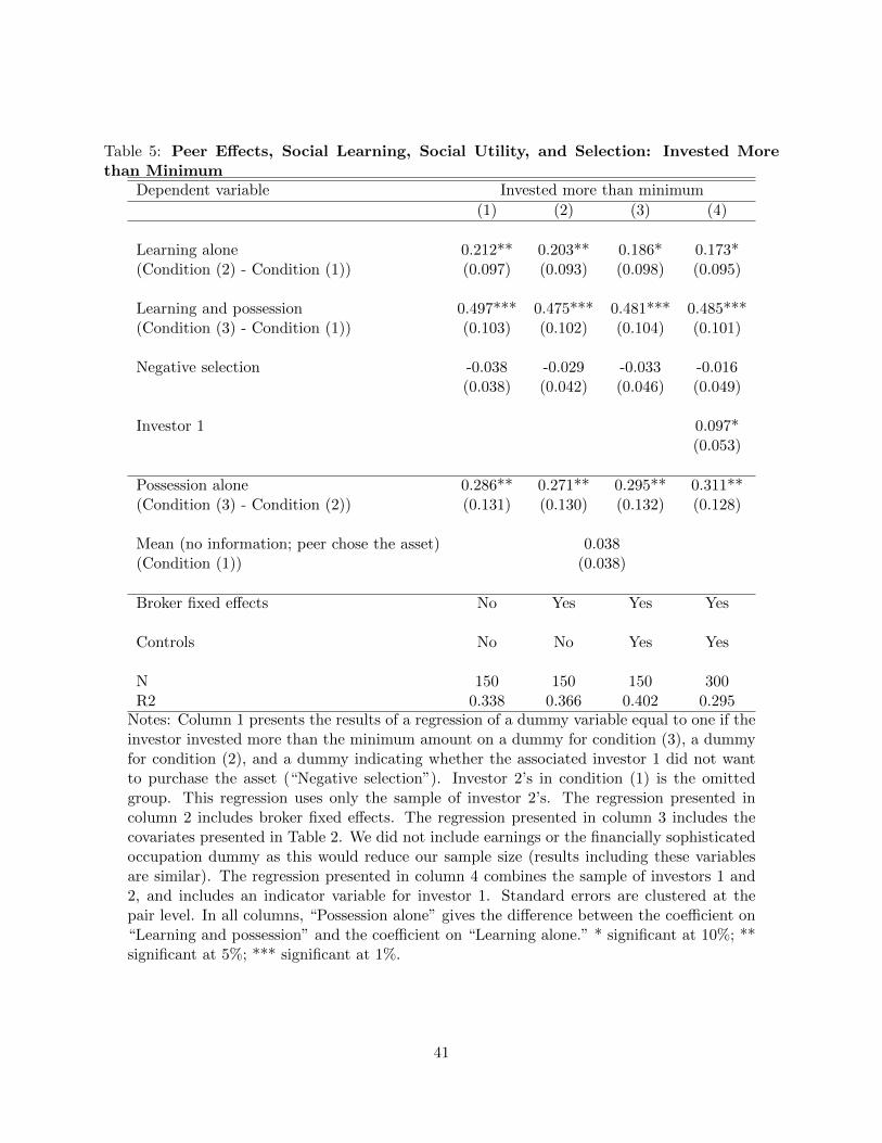
Table 5: Peer Effects, Social Learning, Social Utility, and Selection: Invested Morethan Minimum

Dependent variable Invested more than minimum

(1) (2) (3) (4)

Learning alone 0.212** 0.203** 0.186* 0.173*(Condition (2) - Condition (1)) (0.097) (0.093) (0.098) (0.095)

Learning and possession 0.497*** 0.475*** 0.481*** 0.485***(Condition (3) - Condition (1)) (0.103) (0.102) (0.104) (0.101)

Negative selection -0.038 -0.029 -0.033 -0.016(0.038) (0.042) (0.046) (0.049)

Investor 1 0.097*(0.053)

Possession alone 0.286** 0.271** 0.295** 0.311**(Condition (3) - Condition (2)) (0.131) (0.130) (0.132) (0.128)

Mean (no information; peer chose the asset) 0.038(Condition (1)) (0.038)

Broker fixed effects No Yes Yes Yes

Controls No No Yes Yes

N 150 150 150 300R2 0.338 0.366 0.402 0.295

Notes: Column 1 presents the results of a regression of a dummy variable equal to one if theinvestor invested more than the minimum amount on a dummy for condition (3), a dummyfor condition (2), and a dummy indicating whether the associated investor 1 did not wantto purchase the asset (“Negative selection”). Investor 2’s in condition (1) is the omittedgroup. This regression uses only the sample of investor 2’s. The regression presented incolumn 2 includes broker fixed effects. The regression presented in column 3 includes thecovariates presented in Table 2. We did not include earnings or the financially sophisticatedoccupation dummy as this would reduce our sample size (results including these variablesare similar). The regression presented in column 4 combines the sample of investors 1 and2, and includes an indicator variable for investor 1. Standard errors are clustered at thepair level. In all columns, “Possession alone” gives the difference between the coefficient on“Learning and possession” and the coefficient on “Learning alone.” * significant at 10%; **significant at 5%; *** significant at 1%.

41

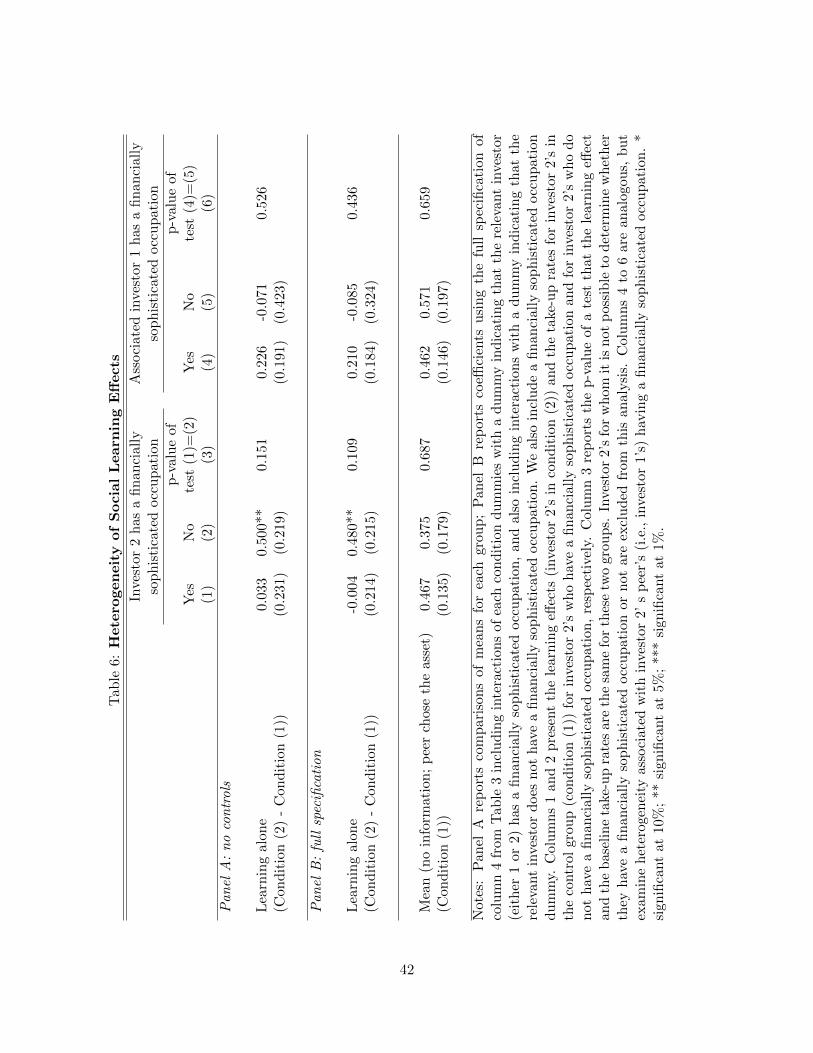
Tab

le6:

Hete

rogen

eit

yof

Socia

lL

earn

ing

Eff

ects

Inve

stor

2h

asa

fin

anci

ally

Ass

oci

ated

inve

stor

1h

as

afi

nanci

ally

sop

his

tica

ted

occ

up

atio

nso

ph

isti

cate

docc

up

ati

on

p-v

alu

eof

p-v

alu

eof

Yes

No

test

(1)=

(2)

Yes

No

test

(4)=

(5)

(1)

(2)

(3)

(4)

(5)

(6)

Pan

elA

:n

oco

ntr

ols

Lea

rnin

gal

one

0.03

30.

500*

*0.

151

0.22

6-0

.071

0.5

26

(Con

dit

ion

(2)

-C

ond

itio

n(1

))(0

.231

)(0

.219

)(0

.191

)(0

.423

)

Pan

elB

:fu

llsp

ecifi

cati

on

Lea

rnin

gal

one

-0.0

040.

480*

*0.

109

0.21

0-0

.085

0.4

36

(Con

dit

ion

(2)

-C

ond

itio

n(1

))(0

.214

)(0

.215

)(0

.184

)(0

.324

)

Mea

n(n

oin

form

atio

n;

pee

rch

ose

the

asse

t)0.

467

0.37

50.

687

0.46

20.

571

0.6

59

(Con

dit

ion

(1))

(0.1

35)

(0.1

79)

(0.1

46)

(0.1

97)

Not

es:

Pan

elA

rep

orts

com

par

ison

sof

mea

ns

for

each

grou

p;

Pan

elB

rep

orts

coeffi

cien

tsu

sin

gth

efu

llsp

ecifi

cati

on

of

colu

mn

4fr

omT

able

3in

clu

din

gin

tera

ctio

ns

ofea

chco

nd

itio

nd

um

mie

sw

ith

adu

mm

yin

dic

atin

gth

at

the

rele

vant

inves

tor

(eit

her

1or

2)h

asa

fin

anci

ally

sop

his

tica

ted

occ

up

atio

n,

and

also

incl

ud

ing

inte

ract

ion

sw

ith

ad

um

my

ind

icati

ng

that

the

rele

vant

inve

stor

does

not

hav

ea

fin

anci

ally

sop

his

tica

ted

occ

up

atio

n.

We

also

incl

ud

ea

fin

anci

ally

sop

his

tica

ted

occ

up

ati

on

du

mm

y.C

olu

mn

s1

and

2p

rese

nt

the

lear

nin

geff

ects

(inve

stor

2’s

inco

nd

itio

n(2

))an

dth

eta

ke-u

pra

tes

for

inve

stor

2’s

inth

eco

ntr

olgr

oup

(con

dit

ion

(1))

for

inve

stor

2’s

wh

oh

ave

afi

nan

cial

lyso

ph

isti

cate

docc

up

atio

nan

dfo

rin

vest

or

2’s

wh

od

on

oth

ave

afi

nan

cial

lyso

ph

isti

cate

docc

up

atio

n,

resp

ecti

vel

y.C

olu

mn

3re

por

tsth

ep

-val

ue

ofa

test

that

the

learn

ing

effec

tan

dth

eb

asel

ine

take

-up

rate

sar

eth

esa

me

for

thes

etw

ogr

oup

s.In

vest

or2’

sfo

rw

hom

itis

not

pos

sib

leto

det

erm

ine

wh

eth

erth

eyh

ave

afi

nan

cial

lyso

ph

isti

cate

docc

up

atio

nor

not

are

excl

ud

edfr

omth

isan

alysi

s.C

olu

mn

s4

to6

are

analo

gou

s,b

ut

exam

ine

het

erog

enei

tyas

soci

ated

wit

hin

vest

or2’

sp

eer’

s(i

.e.,

inve

stor

1’s)

hav

ing

afi

nan

cial

lyso

ph

isti

cate

docc

upati

on

.*

sign

ifica

nt

at10

%;

**si

gnifi

cant

at5%

;**

*si

gnifi

cant

at1%

.

42

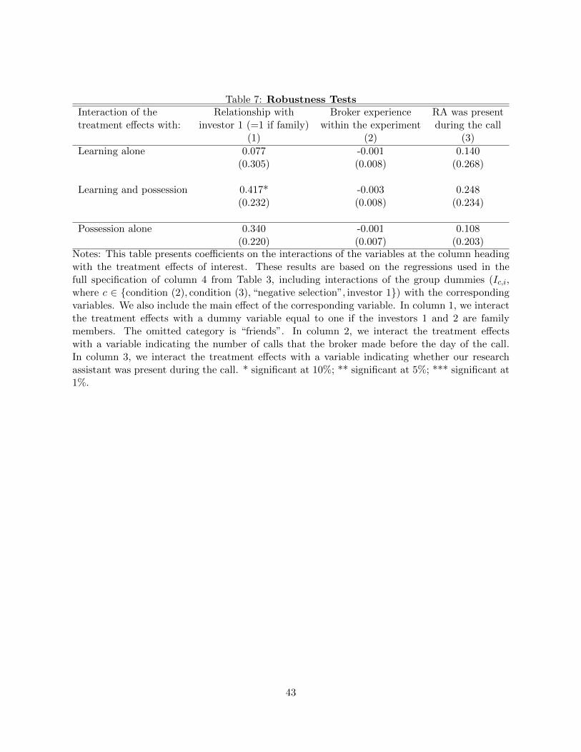
Table 7: Robustness TestsInteraction of the Relationship with Broker experience RA was presenttreatment effects with: investor 1 (=1 if family) within the experiment during the call

(1) (2) (3)

Learning alone 0.077 -0.001 0.140(0.305) (0.008) (0.268)

Learning and possession 0.417* -0.003 0.248(0.232) (0.008) (0.234)

Possession alone 0.340 -0.001 0.108(0.220) (0.007) (0.203)

Notes: This table presents coefficients on the interactions of the variables at the column headingwith the treatment effects of interest. These results are based on the regressions used in thefull specification of column 4 from Table 3, including interactions of the group dummies (Ic,i,where c ∈ {condition (2), condition (3), “negative selection”, investor 1}) with the correspondingvariables. We also include the main effect of the corresponding variable. In column 1, we interactthe treatment effects with a dummy variable equal to one if the investors 1 and 2 are familymembers. The omitted category is “friends”. In column 2, we interact the treatment effectswith a variable indicating the number of calls that the broker made before the day of the call.In column 3, we interact the treatment effects with a variable indicating whether our researchassistant was present during the call. * significant at 10%; ** significant at 5%; *** significant at1%.

43

ONLINE APPENDIX

(NOT FOR PUBLICATION)

Appendix A: A Simple Model of Financial Decisions Under Social

Influence

Our model studies an investment decision made by an individual under several conditions. First,

we present the investment decision under uncertainty, but with no social influence. Second, we

present the investment decision with social learning present, using the ingredients of a canonical

social learning model: a peer makes an investment acting on a private signal, and this action can be

used by another investor to make an informational inference before taking his own action. Third,

we allow the ownership of an asset to affect a socially-related investor’s utility of owning the asset,

aside from any learning – that is, we allow for a social utility effect. A peer’s purchase decision

typically will produce both social learning and social utility effects; we consider a case in which

both effects are active (the full “peer effect”) and a case in which the revealed preference purchase

decision is de-coupled from possession. This de-coupling allows one to observe each channel through

which peer effects work, and motivates our experimental design.

Investment without Peer Effects

Consider an investor i’s decision to invest in a risky asset.71 The asset’s return is given by x, with

probability density function f(x), and investor i’s utility is ui(x) = u(x) for all i. In our field

experiment, investors received calls from brokers who offered them a financial asset for purchase.

The brokers attempted to convey the same information about the asset in every call using a pre-

specified script; thus, the information they provided can be thought of as a signal, si, coming from

a single distribution, with probability density function g(si). Importantly, not every investor would

have received exactly the same information: calls evolve in different ways, investors ask different

71Note that we implicitly assume that when investing in isolation, investor i does not take into consideration anyinvestor j (j 6= i) at all – he is “unaware.” In the context of our experiment, we believe that this assumption isreasonable, as we discuss in the text.

44

questions about the asset, etc., meaning that each investor received a different signal realization,

si, from the common distribution of signals.

For expositional simplicity, assume that the conditional density f(x|si) satisfies the monotone

likelihood ratio property (MLRP) such that, intuitively, higher values of si are indicative of higher

values of x. Under these conditions, investor i is willing to invest if and only if

∫u(x)f(x|si)dx ≥ u, (2)

where u denotes the outside option of the investor. Given that f(x|si) satisfies MLRP and given

mild monotonicity assumptions on the utility function u(·) of the investor, there exists a unique

threshold s1 such that for any si ≥ s1 investor i is willing to invest. Denote the decision to buy

the asset made by investor i by bi = {0, 1}. Hence, for an investor making a purchase decision in

isolation, we have

bi = 1⇔ si ≥ s1. (3)

Investment with Social Learning Alone

Suppose that instead of making his investment choice in isolation, before making his own decision,

investor i observes the investment decision of investor j which is given by bj . Assume that investor

j made his choice bj = 1 in isolation and hence his decision rule is given by (3).72 Thus, when

investor i observes bj = 1 he correctly infers that sj ≥ s1 and he is willing to invest if and only if

∫u(x)f(x|si; sj ≥ s1)dx ≥ u. (4)

Furthermore, given that f(x|si; sj) satisfies MLRP we have

∫u(x)f(x|si; sj ≥ s1)dx ≥

∫u(x)f(x|si)dx, (5)

72We focus on the case of investor i observing that investor j chose to purchase the asset (rather than choosing notto purchase it) because in the experimental design, we were not allowed to inform investors that their peer chose notto purchase the asset.

45

for all si. It is straightforward to show by comparing (4) and (2) that the signal realization threshold

for investor i that is necessary to induce purchase of the asset is lower when bj = 1 is observed than

when investor i makes his choice in isolation. This is because in the former case, regardless of his

own private information summarized by si, investor i has additional favorable information about

the asset from observing the purchase of investor j. This is the pure social learning effect.

Denote the threshold for si when investor i observes bj = 1 by s2 and note that s2 ≤ s1. In

particular, after observing a purchase decision made by investor j, the decision rule of investor i is

given by

bi = 1⇔ si ≥ s2. (6)

Social Utility and Social Learning

We now consider the situation in which both social utility and social learning effects are present.

Our focus (following much of the literature on peer effects in financial decisions) is on social utility

effects that result in a positive effect of a peer’s possession of an asset (denoted by pj = {0, 1})

on one’s own utility.73 In particular, when investor i considers purchasing the asset, we assume

that u(x|pj = 1) ≥ u(x|pj = 0) for all x. That is, investor i’s utility is higher for all asset return

realizations if the asset is also possessed by an investor j who is a peer of investor i. Using the

notation of our model, an investor j’s purchase of an asset, bj = 1, typically implies both that

investor i infers favorable information about the asset, sj ≥ s1, and that investor j now possesses

the asset, pj = 1, which might affect investor i’s utility of owning the asset (due to a taste for joint

consumption, “keeping-up-with-the-Joneses” preferences).

When investor i observes that investor j expressed an intention to invest, bj = 1, and was

allowed to invest, pj = 1, both investor i’s utility u(x|pj = 1) and his information about the asset

f(x|si; sj ≥ s1) are affected, relative to his choice in isolation (that is, relative to u(x) = u(x|pj = 0)

73One could also imagine a negative correlation, for example, out of a desire to insure one’s peers, or to differentiateoneself. See Clark and Oswald (1998).

46

and f(x|si)).74 In this case, one observes the “full” peer effect, and investor i invests if and only if

∫u(x|pj = 1)f(x|si; sj ≥ s1)dx ≥ u. (7)

Denote the threshold for si above which investor i is willing to invest when exposed to both peer

effects channels by s3. Then, the decision rule for investor i is given by

bi = 1⇔ si ≥ s3. (8)

To separate the effects of social learning and social utility, we need to decouple willingness

to purchase (and the informative signal of the purchase decision) from possession. Consider the

situation where investor i observes that investor j expressed a revealed preference to invest, but was

not allowed to do so (perhaps due to capacity constraints). In this case, investor i infers that sj ≥ s1,

but also knows that investor j did not obtain the asset, so pj = 0. This condition is equivalent

to the “social learning alone” problem discussed above: there is no direct effect of possession on

investor i’s utility from the asset, but there is social learning. Thus, investor i purchases the asset

if and only if (4) is satisfied (since u(x) = u(x|pj = 0)) and this leads to the same decision rule as

(6) with the threshold s2.

The following proposition summarizes investor i’s purchase decisions across conditions.

Proposition 1. The threshold for the signal si above which investor i is willing to purchase the

asset (and, the likelihood of a purchase of the asset by investor i) is highest (lowest) when the

investor makes his decision in isolation, lower (higher) when he observes that investor j intended

to purchase the asset but did not obtain it, and lowest (highest) when investor j intended to purchase

the asset, and obtained it: s1 ≥ s2 ≥ s3 (and Pr(si ≥ s3) ≥ Pr(si ≥ s2) ≥ Pr(si ≥ s1)).

Proof. The relationship between s1 and s2 follows immediately from comparing the inequalities

(2) and (4) and the monotone likelihood ratio property of f(x|si; sj). Similarly, comparison of the

inequalities (4) and (7) and u(x) = u(x|pj = 0) ≤ u(x|pj = 1) establishes that s2 ≥ s3. Finally,

74We are assuming here that the utility function discussed above, u(x), is the same as u(x|pj = 0) here. In addition,we are assuming that investor j made his decision in isolation.

47

Pr(si ≥ s3) ≥ Pr(si ≥ s2) ≥ Pr(si ≥ s1) follows from the ranking of the thresholds. �

The difference between s2 and s3 is the result of a difference in investor j’s possession of the

asset.75 In one situation investor j received favorable information and expressed an intent to

purchase the asset, but was unable to execute the purchase due to supply restrictions. In the other

situation investor j received a favorable signal and was also able to obtain the asset. Thus, in

the two cases investor i infers the same information (via investor j’s choice) about the potential

returns of asset x. However, only in the latter case is investor i’s utility directly influenced by the

investment outcome (and not just the purchase intention) of investor j. This is the social utility

effect that raises the expected utility of purchasing the asset for investor i over and above the social

learning effect. In the inequalities in Proposition 1, the effect of social learning is captured by the

difference between Pr(si ≥ s2) and Pr(si ≥ s1), and the effect of social utility is the difference

between Pr(si ≥ s3) and Pr(si ≥ s2). The total peer effect is the difference between Pr(si ≥ s3)

and Pr(si ≥ s1).

Our analysis readily extends to the case in which investor i’s investment choice is continuous

rather than limited to a binary decision. In particular, since f(x|si; sj) satisfies MLRP, the optimal

investment in the asset is increasing in si and sj and the expected equilibrium investment amounts

will follow exactly the prediction regarding purchase rates in Proposition 1. Suppose individual

i chooses an investment magnitude q∗i , rather than making a binary investment decision. Since

f(x|si; sj) satisfies MLRP, the optimal investment in the asset is increasing in si and sj and we can

rank the expected equilibrium investment amounts.

Proposition 2. The expected equilibrium investment amount q∗i of investor i is lowest when the

investor makes his decision in isolation, higher when he observes that investor j intended to purchase

the asset but did not obtain it, and highest when investor j intended to purchase, and obtained, the

asset.

75Note that the difference between s2 and s3 measures the impact of possession conditional on the presence ofsocial learning. This is consistent with our experimental design, in which we are not able to measure the impact ofpossession in the absence of social learning.

48

Proof. The inference problem of investor i is the same as in Proposition 1. Thus, for a given

signal si the described relationship holds for the actual equilibrium investment amount and follows

immediately from comparing the expression for the utilities on the left-hand side of the inequalities

(2), (4) and (7) and by noting that the optimal investment amount is increasing in si and sj .

Finally, taking expectations over the signal realizations si yields the ranking in expected investment

amounts. �

Heterogeneous Investors

In practice, some investors are more financially sophisticated than others, and one would expect

that this variation will affect the peer effects we study here – especially the impact of social learning.

In particular, an unsophisticated investor may have much more to learn about an asset from the

purchase decision of their peer than does a sophisticated investor, as the sophisticated investor likely

has a very good sense of the asset’s quality from his signal alone. Differing financial sophistication

can be captured in our model by allowing the signals si and sj to be drawn from distributions with

differing precision. For simplicity, we make the assumption that, in contrast to unsophisticated

investors, sophisticated investors receive perfectly informative signals. This assumption generates

the following prediction of heterogeneous effects of social learning.

Proposition 3. The thresholds s1 and s2 for the signal si above which investor i is willing to pur-

chase the asset (and hence the likelihood of investor i purchasing the asset) are identical if investor

i is financially sophisticated (i.e., signal si is perfectly informative). If investor j is sophisticated,

then investor i follows the choice of investor j when observing the decision of investor j.

Proof. If si is perfectly informative (i.e., investor i is sophisticated), then si is a sufficient statistic

for x. As a result, sj , and hence the purchase decision of investor j, has no informational value for

sophisticated investor i and does not influence the threshold s1. Hence, s1 = s2. If sj is perfectly

informative, then investor j knows the value of x and makes a perfectly informed investment

decision. As a result, investor i follows investor j’s choice. �

49

Proposition 3 suggests that social learning will be limited (in fact, given the simplifying as-

sumptions made, will be nonexistent) for sophisticated investors. These investors are sufficiently

well-informed that they are not influenced by the revealed preference of another investor. The

proposition further shows that social learning will have relatively strong effects on investment

choices if the investor whose choice is observed is sophisticated.76

76We have assumed that sophisticated investors receive perfectly informative signals. Our results can be extendedto the case in which sophisticated investors receive more informative, but still imperfectly informative, signals.While results for general distributions of x, si and sj that satisfy MLRP do not exist, it is straightforward to showthat for binary signal structures, the impact of social learning will be relatively small when the observing investor issophisticated and relatively large when the observed investor is sophisticated. Finally, it is worth noting that, anotherinvestor’s possession of the asset could still affect financially sophisticated investors’ choices; similarly a financiallyunsophisticated investor’s purchase decision – when accompanied by possession – could influence a peer’s choice.Both of these effects would work through the social utility channel. Thus, we emphasize that these predictions ofheterogeneous treatment effects apply to social learning effects alone, but not necessarily the overall peer effect.

50

Appendix B: Appendix Figures and Tables

Figure A.1: Heterogeneity of Social Learning Effects

Figure A.1.1: Investor 2 has a financially sophisticated occupation

47% 50%38%

88%

Yes No

0.1

.2.3

.4.5

.6.7

.8.9

1

Condition (1) Condition (2) Condition (1) Condition (2)Group

Figure A.1.2: Associated investor 1 has a financially sophisticated occupation

46%68%

57% 50%

Yes No

0.1

.2.3

.4.5

.6.7

.8.9

1

Condition (1) Condition (2) Condition (1) Condition (2)Group

Note: Figure A.1.1 presents the mean (and 95% confidence intervals) of take-up rates for investor 2’s in conditions (1) and

(2), separately for those who have and who do not have a financially sophisticated occupation. Figure A.1.2 presents the take-

up rates separately for those whose associated investor 1’s have and who do not have a financially sophisticated occupation.

Investors in conditions (1) and (2) have peers who wanted the asset. Those in condition (1) had no information about their

peers. Those in condition (2) had information that their peers wanted to purchase the asset but had that choice rejected by

the lottery.

51

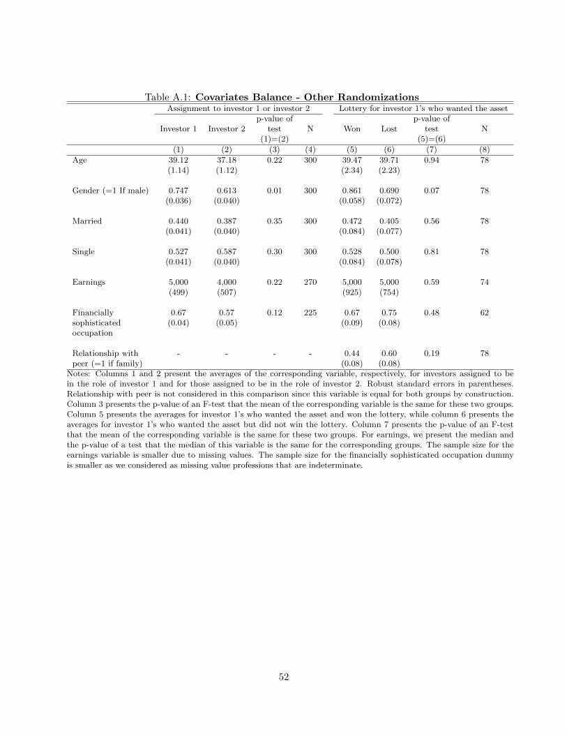
Table A.1: Covariates Balance - Other RandomizationsAssignment to investor 1 or investor 2 Lottery for investor 1’s who wanted the asset

p-value of p-value ofInvestor 1 Investor 2 test N Won Lost test N

(1)=(2) (5)=(6)

(1) (2) (3) (4) (5) (6) (7) (8)

Age 39.12 37.18 0.22 300 39.47 39.71 0.94 78(1.14) (1.12) (2.34) (2.23)

Gender (=1 If male) 0.747 0.613 0.01 300 0.861 0.690 0.07 78(0.036) (0.040) (0.058) (0.072)

Married 0.440 0.387 0.35 300 0.472 0.405 0.56 78(0.041) (0.040) (0.084) (0.077)

Single 0.527 0.587 0.30 300 0.528 0.500 0.81 78(0.041) (0.040) (0.084) (0.078)

Earnings 5,000 4,000 0.22 270 5,000 5,000 0.59 74(499) (507) (925) (754)

Financially 0.67 0.57 0.12 225 0.67 0.75 0.48 62sophisticated (0.04) (0.05) (0.09) (0.08)occupation

Relationship with - - - - 0.44 0.60 0.19 78peer (=1 if family) (0.08) (0.08)

Notes: Columns 1 and 2 present the averages of the corresponding variable, respectively, for investors assigned to bein the role of investor 1 and for those assigned to be in the role of investor 2. Robust standard errors in parentheses.Relationship with peer is not considered in this comparison since this variable is equal for both groups by construction.Column 3 presents the p-value of an F-test that the mean of the corresponding variable is the same for these two groups.Column 5 presents the averages for investor 1’s who wanted the asset and won the lottery, while column 6 presents theaverages for investor 1’s who wanted the asset but did not win the lottery. Column 7 presents the p-value of an F-testthat the mean of the corresponding variable is the same for these two groups. For earnings, we present the median andthe p-value of a test that the median of this variable is the same for the corresponding groups. The sample size for theearnings variable is smaller due to missing values. The sample size for the financially sophisticated occupation dummyis smaller as we considered as missing value professions that are indeterminate.

52

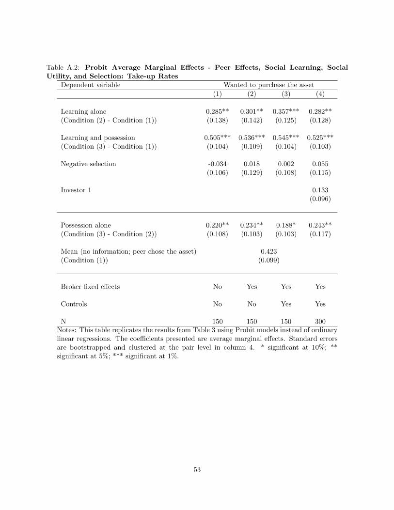
Table A.2: Probit Average Marginal Effects - Peer Effects, Social Learning, SocialUtility, and Selection: Take-up Rates

Dependent variable Wanted to purchase the asset

(1) (2) (3) (4)

Learning alone 0.285** 0.301** 0.357*** 0.282**(Condition (2) - Condition (1)) (0.138) (0.142) (0.125) (0.128)

Learning and possession 0.505*** 0.536*** 0.545*** 0.525***(Condition (3) - Condition (1)) (0.104) (0.109) (0.104) (0.103)

Negative selection -0.034 0.018 0.002 0.055(0.106) (0.129) (0.108) (0.115)

Investor 1 0.133(0.096)

Possession alone 0.220** 0.234** 0.188* 0.243**(Condition (3) - Condition (2)) (0.108) (0.103) (0.103) (0.117)

Mean (no information; peer chose the asset) 0.423(Condition (1)) (0.099)

Broker fixed effects No Yes Yes Yes

Controls No No Yes Yes

N 150 150 150 300Notes: This table replicates the results from Table 3 using Probit models instead of ordinarylinear regressions. The coefficients presented are average marginal effects. Standard errorsare bootstrapped and clustered at the pair level in column 4. * significant at 10%; **significant at 5%; *** significant at 1%.

53

Table A.3: List of occupationsFinancially # of investors Percentage

Occupation sophisticated in the agreementoccupation? sample

Engineer Yes 39 70%Business administrator Yes 34 100%Lawyer Yes 15 70%Entrepreneur Yes 11 70%Bank employee or clerk Yes 8 90%Accountant Yes 6 100%Professor Yes 6 60%Economist Yes 5 100%Real estate, insurance or securities broker Yes 5 100%Capitalist receiving income from invested capital Yes 2 100%Insurance professional Yes 2 100%Commercial establishment owner Yes 2 90%Manager Yes 2 90%Industrial establishment owner Yes 1 90%Actuary or mathematician Yes 1 100%Member of the judiciary: federal supreme court justice Yes 1 70%Medical doctor No 13 60%Teacher No 7 90%Military No 6 90%Journalist No 5 80%Architect No 5 90%Systems analyst No 4 60%Retail or wholesale salesperson No 4 70%Advertising agent No 3 80%Physical therapist or occupational therapist No 3 90%Administrative agent No 3 60%Aircraft pilot No 3 80%State public servant No 3 100%Office assistant or similar occupation No 2 80%Technical specialist No 2 100%Federal public servant No 2 80%Nurse or nutritionist No 2 90%Dentist No 2 70%Pharmacist No 2 80%Professional athlete or sports coach No 1 90%Electricity, electronics or telecommunications technician No 1 100%Chemical technician No 1 90%Speech therapy No 1 90%Public relations No 1 90%Interior designer No 1 90%Maid No 1 100%Psychologist No 1 90%Laboratory or X-ray technician No 1 90%Designer No 1 90%Professional driver No 1 100%Social worker No 1 90%Communications specialist No 1 90%Librarian, archivist, museologist or archeologist No 1 90%Student Undetermined 31 -Other Undetermined 29 -Retired Undetermined 14 -Coordinator or supervisor Undetermined 1 50%

Notes: The financially sophisticated occupation coding is based on a survey with 10 UCLA and UC Berkeley students, who

were asked to classify each occupation in this list as financially sophisticated or not. An occupation was then defined as finan-

cially sophisticated (not financially sophisticated) if 6 or more students classified it as financially sophisticated (not financially

sophisticated). Otherwise, the occupation was classified as undetermined. Categories that are not occupations (student, retired,

and other) were also coded as undetermined.

54

Tab

leA

.4:

Hete

rogen

eit

yof

Socia

lL

earn

ing

Eff

ects

-O

ther

Ou

tcom

es

Inve

stor

2h

asa

fin

anci

ally

Ass

oci

ated

inve

stor

1h

as

afin

an

ciall

yso

ph

isti

cate

docc

up

atio

nso

ph

isti

cate

docc

up

ati

on

p-v

alu

eof

p-v

alu

eof

Yes

No

test

(1)=

(2)

Yes

No

test

(4)=

(5)

(1)

(2)

(3)

(4)

(5)

(6)

Pan

elA

:A

mou

nt

Inve

sted

Lea

rnin

gal

one

-73.

71,

034.

6*0.

201

398.

0-1

,084

.80.1

32

(Con

dit

ion

(2)

-C

ond

itio

n(1

))(7

21.7

)(5

45.1

)(5

65.9

)(8

38.8

)

Mea

n(n

oin

form

atio

n;

pee

rch

ose

the

asse

t)1,

000.

075

0.0

0.59

61,

000.

01,

142.

90.7

83

(Con

dit

ion

(1))

(296

.0)

(358

.3)

(324

.3)

(394

.3)

Pan

elB

:In

vest

edM

ore

than

Min

imu

m

Lea

rnin

gal

one

0.01

90.

355*

*0.

127

0.05

1-0

.116

0.4

08

(Con

dit

ion

(2)

-C

ond

itio

n(1

))(0

.141

)(0

.158

)(0

.133

)(0

.152

)

Mea

n(n

oin

form

atio

n;

pee

rch

ose

the

asse

t)0.

067

0.00

00.

334

0.07

70.

000

0.3

37

(Con

dit

ion

(1))

(0.0

67)

(0.0

00)

(0.0

78)

(0.0

00)

Not

es:

Th

ista

ble

rep

lica

tes

the

resu

lts

from

Pan

elB

ofT

able

6u

sin

gtw

oal

tern

ativ

eou

tcom

es.

Pan

elA

rep

ort

sco

effici

ents

usi

ng

amou

nt

inve

sted

asd

epen

den

tva

riab

le.

Pan

elB

rep

orts

coeffi

cien

tsu

sin

ga

du

mm

yva

riab

leeq

ual

toon

eif

the

inve

stor

inve

sted

mor

eth

anth

em

inim

um

amou

nt

asd

epen

den

tva

riab

le.

*si

gnifi

cant

at10

%;

**si

gnifi

cant

at

5%

;***

sign

ifica

nt

at

1%.

55

Appendix C: Experimental Documentation

We enclose here English versions of the Qualtrics scripts used by the brokers in the phone calls,first to investor 1’s and then to investor 2’s. After these documents, we enclose a picture of theimplementation of the experiment, displaying the brokers and the RA.

56

6/24/12 5:15 PMQualtrics Survey Software

Page 1 of 3

Client number

Name of broker making phone call

Client number

Introduction

Description of asset

Combination of two investments:- Fundo Long-Short multi-mercado (read brochure)- LCI de 98% do CDI (read brochure) Minimum investment:- R$1,000 in LCI and R$1,000 in Fundo Long-ShortMaximum investment:-R$10,000 in LCI and no limits in Fundo Long-Short Observations to be told to client:1) Special LCI usually not avaliable to clients. LCI typically available to clients has return of 97% of CDI andminimum investment of R$10,000

2) Emphasize that product can only be purchased during this call (take it or leave it): will not be sold on otheroccasions

3) Remind that LCI is exempt from income tax

4) Explain that only new resources will be accepted (and not resources already invested with the brokerage)

Limited supply

This is a special asset, only available in limited supply, and only to special clients l ke you.

As so, unfortunately, some of the clients that want the asset will not be able to actually purchase it.

Since we are a company that always wants to be as fair as possible, we want to give a chance to all the specialclients we are calling and who are interested in the product. In addition to that, we would like to give the samechance to everyone.

Because of that, we will use a lottery to determine which clients will actually be able to implement the purchase,among those that chose to purchase the asset.

In this lottery half (50%) of the clients that choose to purchase the asset will have their choices authorized andimplemented.

The lottery consists in drawing a random integer number between 1 and 100. If the number is 50 or less, the lotterywill not authorize the investment. If the number is greater than 50, the lottery will authorize and make the investment.

It is important that you know that the decision you will make now if final. If you decide to purchase the asset, you willbe authorizing the purchase. Therefore, if the lottery authorizes the purchase, the investment will be made.

Take advantage of this great opportunity to buy this exclusive product!

Investment decision

6/24/12 5:15 PMQualtrics Survey Software

Page 2 of 3

Wants to invest

Does not want to invest

Yes

No

Ask the client what their decision is

How much does he want to invest in the Fundo Long-Short multi-mercado?

How much does he want to invest in the LCI?

Investment authorization

A random number will now be drawn to determine whether or not you will be able to actually make the investment.The random number is ${e://Field/random}

Due to the outcome of the lottery, your investment was not authorized.

Due to the outcome of the lottery, your investment was authorized.

Was the investment authorized?

End of Call and Summary

Finish the call

This is the summary of the call. Please put the following information in your Excel spreadsheet of communicationwith the clients:

Client number: ${q://QID20/ChoiceTextEntryValue}

Did this client want to invest in the product? Yes

Amount invested in the Fundo Long-Short: ${q://QID18/ChoiceTextEntryValue}

Amount invested in the LCI: ${q://QID26/ChoiceTextEntryValue}

Was this client authorized to make the investment? Yes

This is the summary of the call. Please put the following information in your Excel spreadsheet of communicationwith the clients:

Client number: ${q://QID20/ChoiceTextEntryValue}

Did this client want to invest in the product? Yes

Amount invested in the Fundo Long-Short: ${q://QID18/ChoiceTextEntryValue}

Amount invested in the LCI: ${q://QID26/ChoiceTextEntryValue}

6/24/12 5:15 PMQualtrics Survey Software

3

Was this client authorized to make the investment? No

This is the summary of the call. Please put the following information in your Excel spreadsheet of communicationwith the clients:

Client number: ${q://QID20/ChoiceTextEntryValue}

Did this client want to invest in the product? No

Amount invested in the Fundo Long-Short: 0

Amount invested in the LCI: 0

Was this client authorized to make the investment? N/A

6/24/12 5:16 PMQualtrics Survey Software

Page 1 of 4

Yes

No

Yes

No

Client number

Name of broker making phone call

Client number

Number of client of the (first) friend of this investor

Previous Choice by FRIEND 1

Did the first friend of this investor want to invest in this asset?

Was the first friend of this investor authorized to make the investment?

Introduction

Description of Asset

Combination of two investments:- Fundo Long-Short multi-mercado (read brochure)- LCI de 98% do CDI (read brochure) Minimum investment:- R$1,000 in LCI and R$1,000 in Fundo Long-ShortMaximum investment:-R$10,000 in LCI and no limits in Fundo Long-Short Observations to be told to client:1) Special LCI usually not avaliable to clients. LCI typically available to clients has return of 97% of CDI andminimuminvestment of R$10,000 2) Emphasize that product can only be purchased during this call (take it or leave it): will not be sold on otheroccasions 3) Remind that LCI is exempt from income tax 4) Explain that only new resources will be accepted (and not resources already invested with the brokerage)

Limited Supply

This is a special asset, only available in limited supply, and only to special clients l ke you.

6/24/12 5:16 PMQualtrics Survey Software

Page 2 of 4

Wants to invest

Does not want to invest

As so, unfortunately, some of the clients that want the asset will not be able to actually purchase it.

Since we are a company that always wants to be as fair as possible, we want to give a chance to all the specialclients we are calling and who are interested in the product. In addition to that, we would like to give the samechance to everyone.

Because of that, we will use a lottery to determine which clients will actually be able to implement the purchase,among those that chose to purchase the asset.

In this lottery half (50%) of the clients that choose to purchase the asset will have their choices authorized andimplemented.

The lottery consists in drawing a random integer number between 1 and 100. If the number is 50 or less, the lotterywillnot authorize the investment. If the number is greater than 50, the lottery will authorize and make the investment.

It is important that you know that the decision you will make now if final. If you decide to purchase the asset, you willbe authorizing the purchase. Therefore, if the lottery authorizes the purchase, the investment will be made.

Take advantage of this great opportunity to buy this exclusive product!

Only Learning Treatment

Before asking whether or not the client wants to purchase the asset, tell him the information associated with thechoice of the first friend and the outcome of the lottery for the first friend: "We would like to inform you, before you make your decision, that [FIRST FRIEND'S NAME], your [RELATIONSHIPTO THIS CLIENT], received the same offer today. He/she chose to purchase the product. However, the lottery didnot authorize him/her to make the purchase, so he/she will not make the investment." SUMMARIZING: He/she wanted to make the investment but was not able to invest.

Possession and Learning Treatment

Before asking whether or not the client wants to purchase the asset, tell him the information associated with thechoice of the first friend and the outcome of the lottery for the first friend:

"We would like to inform you, before you make your decision, that [FIRST FRIEND'S NAME], your [RELATIONSHIPTO THIS CLIENT], received the same offer today. He/she chose to purchase the product. The lottery authorizedhim/her to make the purchase, so he/she will make the investment." SUMMARIZING: He/she wanted to make the investment and was able to invest.

Investment Decision

Ask the client what their decision is

How much does he want to invest in the Fundo Long-Short multi-mercado?

How much does he want to invest in the LCI?

6/24/12 5:16 PMQualtrics Survey Software

Page 3 of 4

Yes

No

Yes

No

Investment Authorization

A random number will now be drawn to determine whether or not you will be able to actually make the investment.The random number is ${e://Field/random}

Due to the outcome of the lottery, your investment was not authorized.

Due to the outcome of the lottery, your investment was authorized.

Was the investment authorized?

Relationship with First Investor, End of Call, and Summary

Had you previously heard about this offer/this product from [FIRST FRIEND'S NAME]?

What is your degree of relationship with [FIRST FRIEND'S NAME]? Examples: sibling, parent, friend, co-worker, etc.

Finish the phone call

This is the summary of the call. Please put the following information in your Excel spreadsheet of communicationwith the clients:

Client number: ${q://QID27/ChoiceTextEntryValue}

First friend's client number: ${q://QID30/ChoiceTextEntryValue}

Did the first friend want to invest in the product? ${q://QID21/ChoiceGroup/SelectedChoices}

Was the first friend authorized to make the investment? ${q://QID25/ChoiceGroup/SelectedChoices}

Did this client (second friend) want to invest in the product? Yes

Amount invested in the Fundo Long-Short: ${q://QID28/ChoiceTextEntryValue}

Amount invested in the LCI: ${q://QID38/ChoiceTextEntryValue}

Was this client authorized to make the investment? Yes

This is the summary of the call. Please put the following information in your Excel spreadsheet of communicationwith the clients:

Client number: ${q://QID27/ChoiceTextEntryValue}

First friend's client number: ${q://QID30/ChoiceTextEntryValue}

Did the first friend want to invest in the product? ${q://QID21/ChoiceGroup/SelectedChoices}

6/24/12 5:16 PMQualtrics Survey Software

Page 4 of 4

Was the first friend authorized to make the investment? ${q://QID25/ChoiceGroup/SelectedChoices}

Did this client (second friend) want to invest in the product? Yes

Amount invested in the Fundo Long-Short: ${q://QID28/ChoiceTextEntryValue}

Amount invested in the LCI: ${q://QID38/ChoiceTextEntryValue}

Was this client authorized to make the investment?: No

This is the summary of the call. Please put the following information in your Excel spreadsheet of communicationwith the clients:

Client number: ${q://QID27/ChoiceTextEntryValue}

First friend's client number: ${q://QID30/ChoiceTextEntryValue}

Did the first friend want to invest in the product? ${q://QID21/ChoiceGroup/SelectedChoices}

Was the first friend authorized to make the investment? ${q://QID25/ChoiceGroup/SelectedChoices}

Did this client (second friend) want to invest in the product? No

Amount invested in the Fundo Long-Short: 0

Amount invested in the LCI: 0

Was this client authorized to make the investment?: N/A

Figure A.2: Picture from the implementation

64