CODEN:LUTEDX/(TEIE-5233/1-40/(2007)

Lund University

Underground cables in transmission networks

Johan Engström

Dept. of Industrial Electrical Engineering and Automation

Indust

rial E

lectr

ical Engin

eering a

nd A

uto

mation

Abstract In our modern society it is almost impossible to get permits for new overhead lines. The power companies struggle against residents that do not want an overhead line in their neighborhood. This struggle takes years and costs a lot of money. A way of dealing with these problems could be to build an underground AC-cable. The buried cable would probably not cause such struggle to get permits. When a cable is installed in an existing transmission grid it carries more load than an overhead line should have carried. The reason behind this is that the cable has lower impedance than overhead lines. This lower impedance has to be compensated in some way. The simplest way is to install a series reactor on the cable which increases the impedance. The amount of reactive power produced by a cable is in the vicinity of 20 times larger than the reactive power produced by an overhead line. This reactive power needs to be taken care of by shunt reactors. The degree of compensation needs to be about 100 %, the degree of compensation is the ratio between created reactive power and shunt compensated reactive power. Most of the reactive power needs to be compensated in order to energize the cable; the voltage would otherwise become higher than the highest voltage for equipment. The Sydlänken case is a 400 km long cable at 400 kV. The degree of compensation is 100 % and there are 14 shunt reactors with 200 Mvar each. In order to decrease the load flow through the cable a phase shifting transformer is installed. The phase shifting transformer can regulate the load flow and thereby increases the stability of the whole power system. In a smaller city network, 130 kV, the cable can produce the amount of reactive power needed in the city. The reactive power feeds the city’s transformers and loads. The city does not need to buy reactive power from the power grid, they can produce the amount needed them self.

Sammanfattning I vårt moderna samhälle är det nästan omöjligt att få tillstånd för nya högspänningsluftledningar. Kraftbolagen har en hård kamp mot alla boende som inte vill ha en högspänningsledning i deras omgivning. Den här kampen tar år och kostar massor av pengar. En möjlig lösning på problemen kan vara att bygga en nedgrävd AC-kabel. En nedgrävd kabel skulle nog inte orsaka lika mycket problem med att få tillstånd. När en kabel installeras i ett befintligt transmissionsnät tar den på sig för mycket last. Anledningen till detta är att kabeln har en mycket lägre impedans jämfört med en luftledning. Den lägre impedansen måste kompenseras på något sätt. Det enklaste sättet är att installera en seriereaktor på kabeln som ökar kabelns impedans. Den mängden reaktiv effekt som produceras av en kabel är i närheten av 20 gånger mer än för en luftledning. Den reaktiva effekten behöver tas om hand av shuntreaktorer som förbrukar reaktiv effekt. Kompenseringsgraden behöver vara 100 %, kompenseringsgraden är förhållandet mellan shuntkompenserad reaktiv effekt och skapad reaktiv effekt. All reaktiv effekt behöver kompenseras när kabeln ska spänningssättas, spänningen skulle annars överstiga konstruktionsspänningen för utrustningen. Sydlänkenfallet har en nominell spänning om 400 kV och är 400 km långt. Kompenseringsgraden är 100 % och det är 14 stycken shuntreaktorer på 200 Mvar per styck. För att kunna minska effektflödet i kabeln installeras en fasvridande transformator. En fasvridande transformator kan reglera effektflödet och därmed hjälpa till att öka stabiliteten för hela kraftsystemet. I ett mindre stadsnät, 130 kV, kan en kabel producera den mängd reaktiv effekt som staden behöver. Den reaktiva effekten matar transformatorer och laster. Staden behöver inte köpa reaktiv effekt från elnätet utan kan skapa den själva.

Preface This master thesis concludes my studies at The Faculty of Engineering (LTH), Lund University, for a master degree in electrical engineering. This thesis work has been conducted in cooperation with ABB and the Department of Industrial Electrical Engineering and Automation (IEA) at Lund University. I would like to thank my tutors Sture Lindahl at IEA and Stefan Thorburn at ABB for the indispensable guidance through this thesis. Lund, 30 January 2007 Johan Engström

……………………………………………..

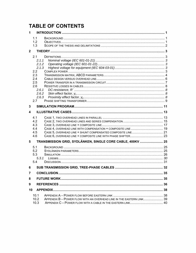
TABLE OF CONTENTS 1 INTRODUCTION .................................................................................................................... 1

1.1 BACKGROUND .................................................................................................................. 1 1.2 OBJECTIVES..................................................................................................................... 1 1.3 SCOPE OF THE THESIS AND DELIMITATIONS ........................................................................ 2

2 THEORY ................................................................................................................................. 3 2.1 DEFINITIONS..................................................................................................................... 3

2.1.1 Nominal voltage (IEC 601-01-21) .............................................................................. 3 2.1.2 Operating voltage (IEC 601-01-22)............................................................................ 3 2.1.3 Highest voltage for equipment (IEC 604-03-01) ........................................................ 3

2.2 COMPLEX POWER ............................................................................................................. 3 2.3 TRANSMISSION MATRIX, ABCD PARAMETERS..................................................................... 4 2.4 CABLE DESIGN VERSUS OVERHEAD LINE............................................................................. 6 2.5 POWER TRANSFER IN A TRANSMISSION CIRCUIT.................................................................. 7 2.6 RESISTIVE LOSSES IN CABLES............................................................................................ 8

2.6.1 DC-resistance, R´ ...................................................................................................... 8 2.6.2 Skin effect factor, y ................................................................................................... 8 s2.6.3 Proximity effect factor, y ........................................................................................... 8 p

2.7 PHASE SHIFTING TRANSFORMER........................................................................................ 9 3 SIMULATION PROGRAM.................................................................................................... 11 4 ILLUSTRATIVE CASES....................................................................................................... 13

4.1 CASE 1, TWO OVERHEAD LINES IN PARALLEL .................................................................... 13 4.2 CASE 2, TWO OVERHEAD LINES AND SERIES COMPENSATION............................................. 15 4.3 CASE 3, OVERHEAD LINE + COMPOSITE LINE..................................................................... 17 4.4 CASE 4, OVERHEAD LINE WITH COMPENSATION + COMPOSITE LINE .................................... 19 4.5 CASE 5, OVERHEAD LINE + SHUNT COMPENSATED COMPOSITE LINE................................... 21 4.6 CASE 6, OVERHEAD LINE + COMPOSITE LINE WITH PHASE SHIFTER..................................... 23

5 TRANSMISSION GRID, SYDLÄNKEN, SINGLE CORE CABLE, 400KV .......................... 25 5.1 BACKGROUND ................................................................................................................ 25 5.2 SYDLÄNKEN PARAMETERS............................................................................................... 25 5.3 SIMULATION ................................................................................................................... 26

5.3.1 Losses...................................................................................................................... 30 5.4 DISCUSSION ................................................................................................................... 31

6 SUB TRANSMISSION GRID, TREE-PHASE CABLES ...................................................... 32 7 CONCLUSION...................................................................................................................... 35 8 FUTURE WORK ................................................................................................................... 35 9 REFERENCES ..................................................................................................................... 36 10 APPENDIX............................................................................................................................ 38

10.1 APPENDIX A – POWER FLOW BEFORE EASTERN LINK ........................................................ 38 10.2 APPENDIX B – POWER FLOW WITH AN OVERHEAD LINE IN THE EASTERN LINK...................... 39 10.3 APPENDIX C – POWER FLOW WITH A CABLE IN THE EASTERN LINK..................................... 40

1 Introduction

1.1 Background

1.2 Objectives

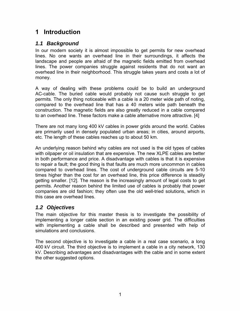
In our modern society it is almost impossible to get permits for new overhead lines. No one wants an overhead line in their surroundings, it affects the landscape and people are afraid of the magnetic fields emitted from overhead lines. The power companies struggle against residents that do not want an overhead line in their neighborhood. This struggle takes years and costs a lot of money. A way of dealing with these problems could be to build an underground AC-cable. The buried cable would probably not cause such struggle to get permits. The only thing noticeable with a cable is a 20 meter wide path of noting, compared to the overhead line that has a 40 meters wide path beneath the construction. The magnetic fields are also greatly reduced in a cable compared to an overhead line. These factors make a cable alternative more attractive. [4] There are not many long 400 kV cables in power grids around the world. Cables are primarily used in densely populated urban areas; in cities, around airports, etc. The length of these cables reaches up to about 50 km. An underlying reason behind why cables are not used is the old types of cables with oilpaper or oil insulation that are expensive. The new XLPE cables are better in both performance and price. A disadvantage with cables is that it is expensive to repair a fault; the good thing is that faults are much more uncommon in cables compared to overhead lines. The cost of underground cable circuits are 5-10 times higher than the cost for an overhead line, this price difference is steadily getting smaller. [12]. The reason is the increasingly amount of legal costs to get permits. Another reason behind the limited use of cables is probably that power companies are old fashion; they often use the old well-tried solutions, which in this case are overhead lines.

The main objective for this master thesis is to investigate the possibility of implementing a longer cable section in an existing power grid. The difficulties with implementing a cable shall be described and presented with help of simulations and conclusions. The second objective is to investigate a cable in a real case scenario, a long 400 kV circuit. The third objective is to implement a cable in a city network, 130 kV. Describing advantages and disadvantages with the cable and in some extent the other suggested options.

1

1.3 Scope of the thesis and delimitations All calculations are made in steady state; therefore additional calculations have to be made in terms of short circuit calculations, dynamic stability, etc. in order to fully investigate the viability of the solution.

2

2 Theory This chapter defines the theory used in this thesis.

2.1 Definitions

2.2

2.1.1 Nominal voltage (IEC 601-01-21) A suitable approximate value of voltage used to designate or identify a system. i.e. 130, 220, and 400 kV. [6]

2.1.2 Operating voltage (IEC 601-01-22) The value of the voltage under normal conditions, at a given instant at a given point of the system. [6]

2.1.3 Highest voltage for equipment (IEC 604-03-01) The highest r.m.s. value of phase-to-phase voltage for which the equipment is designed in respect of its insulation as well as other characteristics which relate to this voltage in the relevant equipment standards. [7]

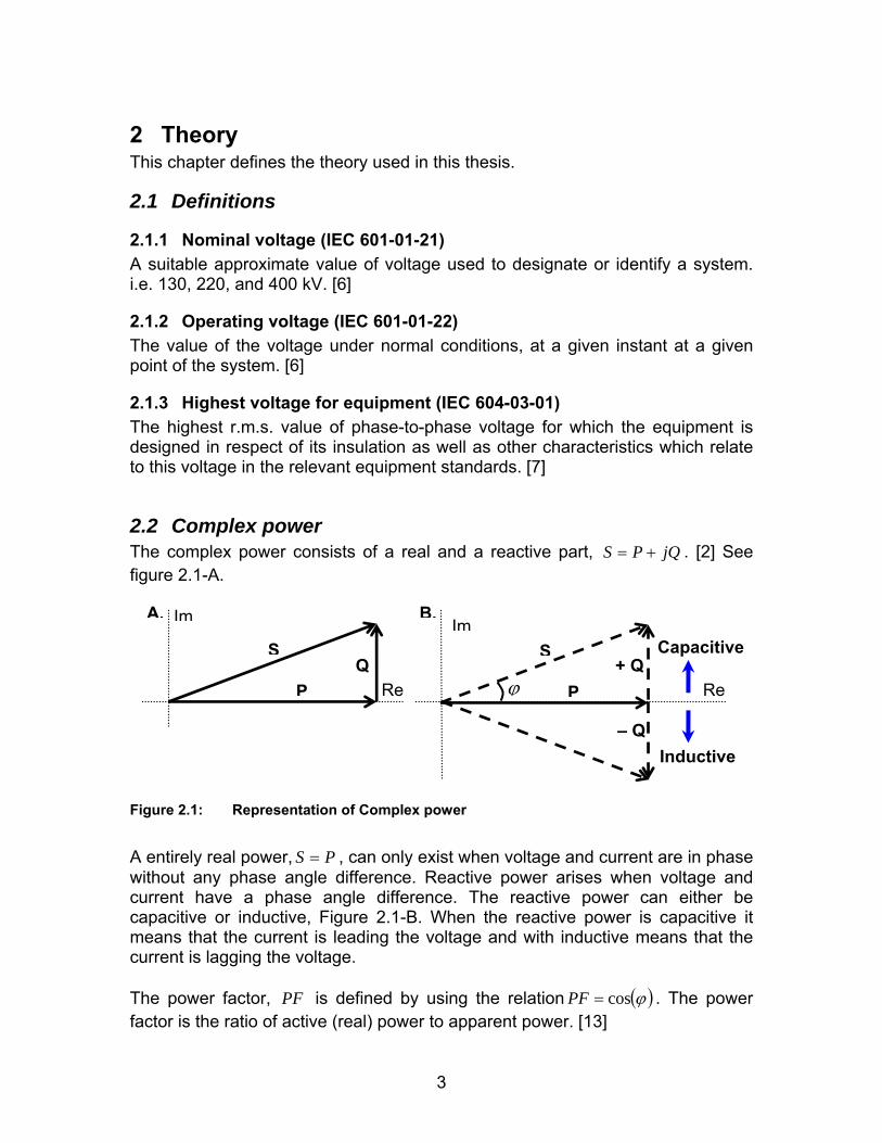
Complex power The complex power consists of a real and a reactive part, . [2] See jQPS +=figure 2.1-A.

S

PQ

S

P+ Q

Im

– Q

Im

Inductive

Re

A. B.

ϕ Re

Capacitive

Figure 2.1: Representation of Complex power

A entirely real power, , can only exist when voltage and current are in phase without any phase angle difference. Reactive power arises when voltage and current have a phase angle difference. The reactive power can either be capacitive or inductive,

PS =

Figure 2.1-B. When the reactive power is capacitive it means that the current is leading the voltage and with inductive means that the current is lagging the voltage.

( )ϕcos=PFPFThe power factor, is defined by using the relation . The power factor is the ratio of active (real) power to apparent power. [13]

3

2.3 Transmission matrix, ABCD parameters To calculate voltages and currents, long circuit theory with ABCD parameters is used in this thesis. The transmission matrix, ABCD parameters, makes it easy to connect different blocks of parameters together, either in series or in parallel. Equation 2.1 defines the parameterizations of a circuit. [13] (Derived from propagation constants in steady state).

( ) ( )( ) ( ) ⎥

⎦

⎤⎢⎣

⎡

⎥⎥⎦

⎤

⎢⎢⎣

⎡

⋅⋅⋅⋅⋅⋅

=⎥⎦

⎤⎢⎣

⎡⎥⎦

⎤⎢⎣

⎡=⎥

⎦

⎤⎢⎣

⎡

R

R

C

C

R

R

S

S

IV

lyzlyzYlyzZlyz

IV

DCBA

IV

coshsinhsinhcosh

Equation 2.1

yz1Zc ==

CYwhere

SV , The sending end voltage and current SI

RV RI, The receiving end voltage and current

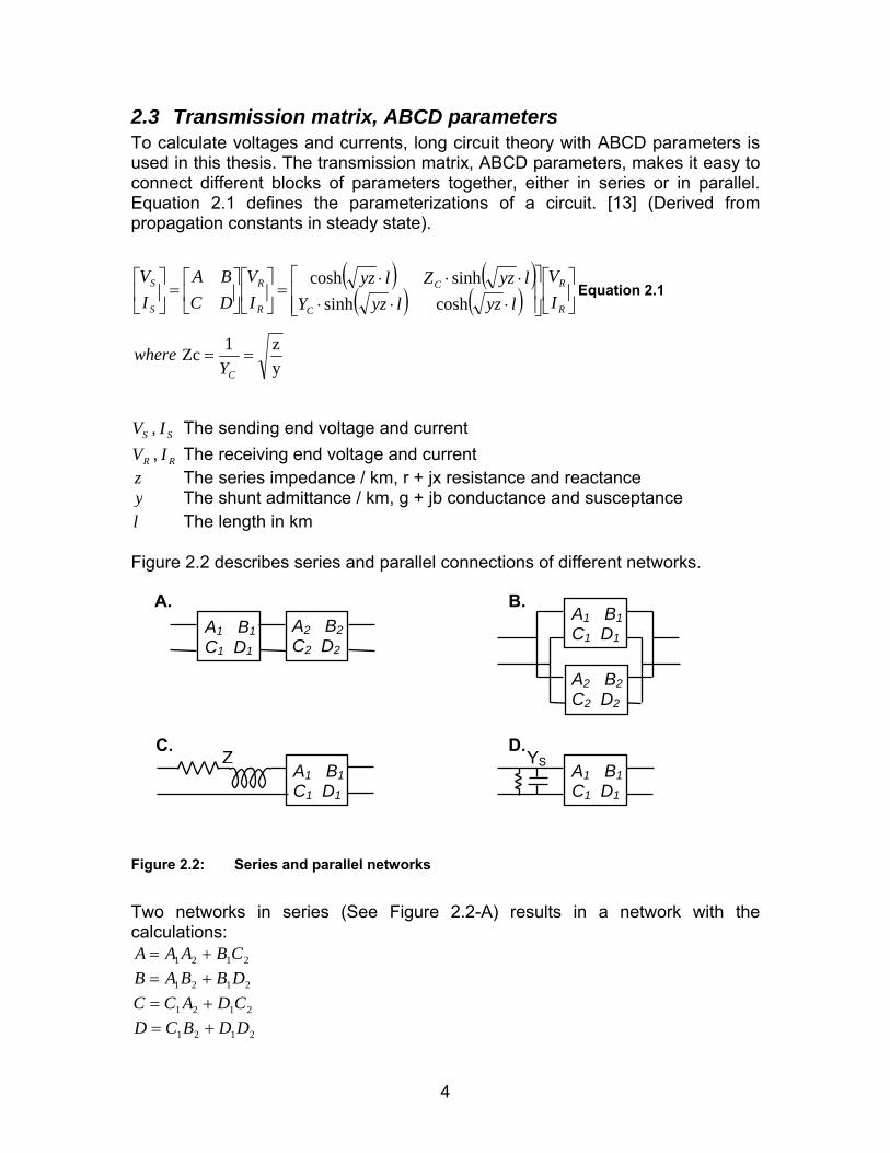
z The series impedance / km, r + jx resistance and reactance y The shunt admittance / km, g + jb conductance and susceptancel The length in km Figure 2.2 describes series and parallel connections of different networks.

A1 B1C1 D1

A. B. A2 B2C2 D2

A1 B1C1 D1

C. A1 B1C1 D1

A2 B2C2 D2

A1 B1C1 D1

D. Z YS

Figure 2.2: Series and parallel networks

Two networks in series (See Figure 2.2-A) results in a network with the calculations:

2121 CBAAA += 2121 DBBAB +=

2121 CDACC +=

2121 DDBCD +=

4

Two networks in parallel (See Figure 2.2-B) results in a network with the calculations:

21

1221

BBBABAA

++

=

21

21

BBBBB+

=

( )( )21

122121 BB

DDAACCC+

−−++=

21

1221

BBBDBDD

++

=

ZA series impedance, at the sending end with a circuit, A B C D1 B1 1 1, (See

-C) results in a network with the calculations: Figure

2.2ZCAA 11 += ZDBB 11 +=

1CC =

1DD = A shunt admittance, at the sending together with a circuit, ASY B C D1 B1 1 1, (See

-D) results in a network with the calculations: Figure 2.21AA =

1BB =

SYACC 11 +=

SYACC 11 +=

5

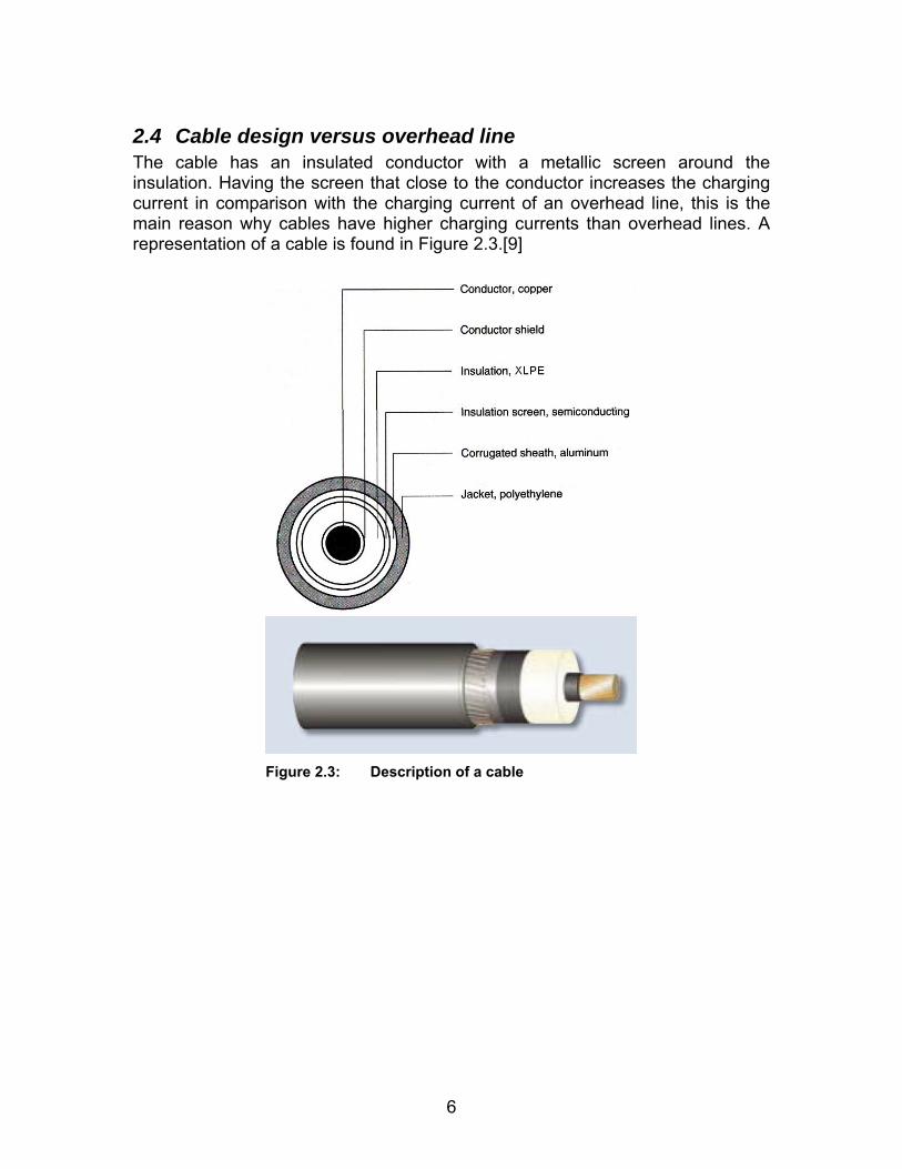
2.4 Cable design versus overhead line The cable has an insulated conductor with a metallic screen around the insulation. Having the screen that close to the conductor increases the charging current in comparison with the charging current of an overhead line, this is the main reason why cables have higher charging currents than overhead lines. A representation of a cable is found in Figure 2.3.[9]

Figure 2.3: Description of a cable

6

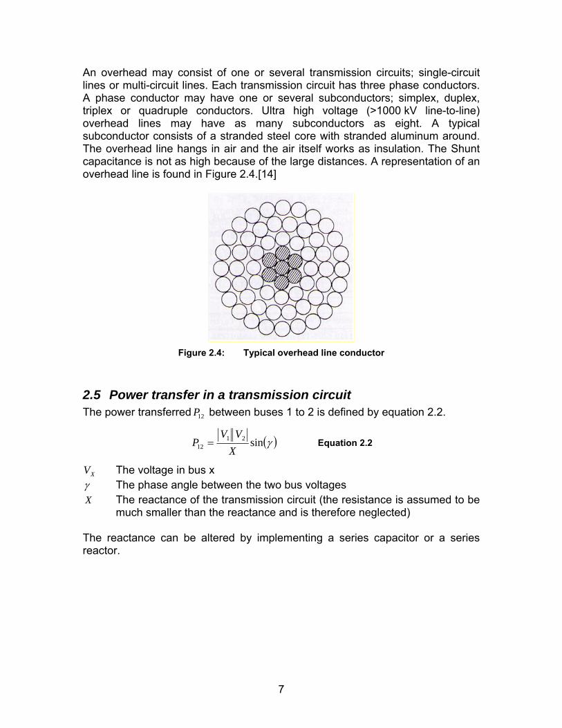
An overhead may consist of one or several transmission circuits; single-circuit lines or multi-circuit lines. Each transmission circuit has three phase conductors. A phase conductor may have one or several subconductors; simplex, duplex, triplex or quadruple conductors. Ultra high voltage (>1000 kV line-to-line) overhead lines may have as many subconductors as eight. A typical subconductor consists of a stranded steel core with stranded aluminum around. The overhead line hangs in air and the air itself works as insulation. The Shunt capacitance is not as high because of the large distances. A representation of an overhead line is found in Figure 2.4.[14]

Figure 2.4: Typical overhead line conductor

2.5 Power transfer in a transmission circuit The power transferred between buses 1 to 2 is defined by 12P equation 2.2.

( )γsin2112 X

VVP = Equation 2.2

XV The voltage in bus x γ The phase angle between the two bus voltages

The reactance of the transmission circuit (the resistance is assumed to be much smaller than the reactance and is therefore neglected)

X

The reactance can be altered by implementing a series capacitor or a series reactor.

7

2.6 Resistive losses in cables In order to calculate the resistive losses, a number of factors have to be calculated. The AC-resistance, R, of a cable is given by equation 2.3.

( )ps yyRR ++= 1´ Equation 2.3

´R DC-resistance at a given temperature sy The skin effect factor, explained in chapter 2.6.2

py The proximity effect factor, explained in chapter 2.6.3

2.6.1 DC-resistance, R´ A conductor resistance is almost always given in the DC-resistance at 20 °C, R0. The resistance is temperature dependant and in order to resolve the DC-resistance at a given temperature, T, equation 2.4 is used. [8]

( )[ ]201´ 200 += TRR −α Equation 2.4

2.6.2 Skin effect factor, y s

The skin effect is the alternating electric current tendency to distribute a greater current density near the surface of the conductor, than at its core. The current flows at the “skin” of the conductor. The skin effect factor is given by equation 2.5. [8]

wherex

xy

s

ss ,

8.0192 4

4

⋅+= ss k

Rfx ⋅⋅= −72 10´

8π Equation 2.5

sk A coefficient depending on the conductor shape

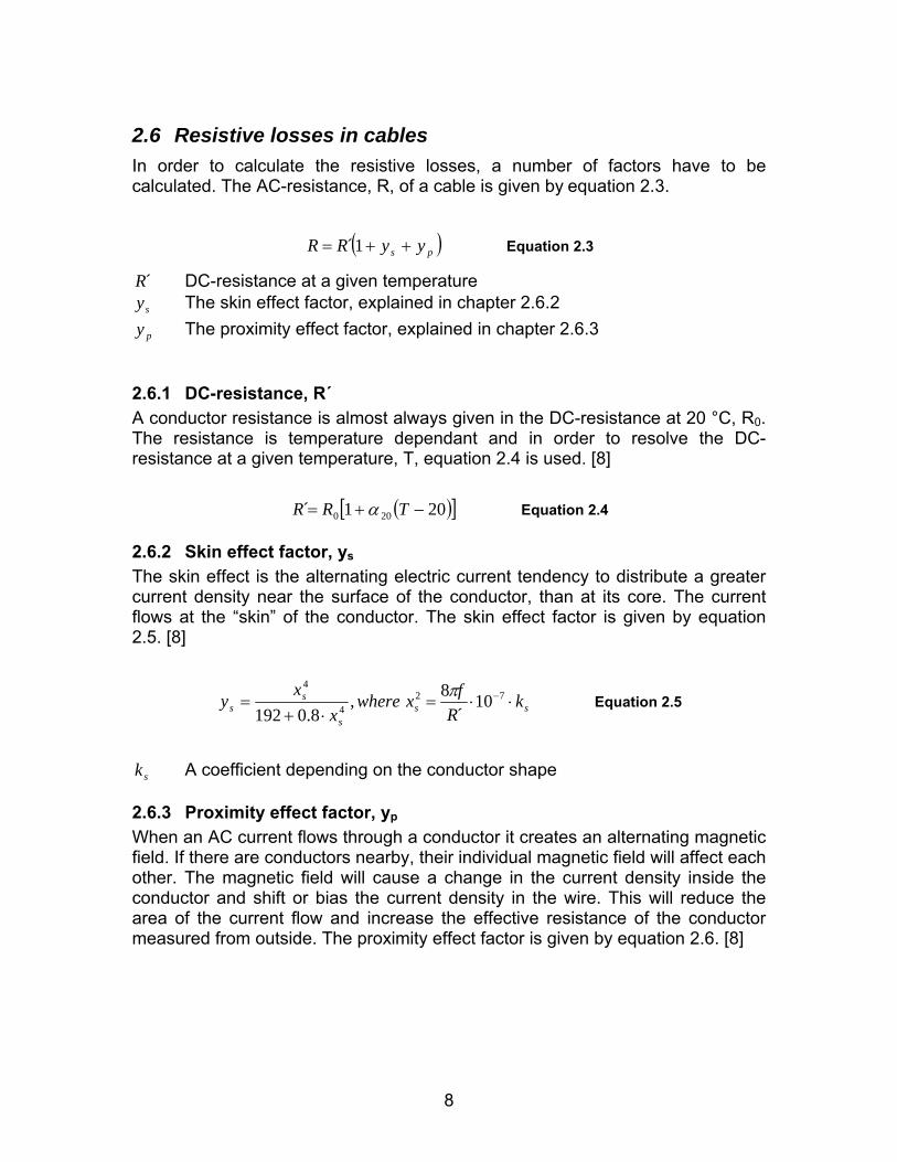
2.6.3 Proximity effect factor, yp When an AC current flows through a conductor it creates an alternating magnetic field. If there are conductors nearby, their individual magnetic field will affect each other. The magnetic field will cause a change in the current density inside the conductor and shift or bias the current density in the wire. This will reduce the area of the current flow and increase the effective resistance of the conductor measured from outside. The proximity effect factor is given by equation 2.6. [8]

8

⎥⎥⎥⎥⎥

⎦

⎤

⎢⎢⎢⎢⎢

⎣

⎡

+⋅+

+⎟⎠⎞

⎜⎝⎛⋅⋅⎟

⎠⎞

⎜⎝⎛⋅

⋅+=

27.08.0192

18.1312.08.0192

4

4

22

4

4

p

p

CC

p

pp

xxs

ds

dx

xy Equation 2.6

PP kR

fx ⋅⋅= −72 10´

8πwhere

Cd The diameter of conductor (mm)

s The distance between conductor axes (mm) pk A coefficient depending on the conductor shape

2.7 Phase shifting transformer A phase shifting transformer, PST, is used for regulating the power flow in a power system. The PST is often placed between two independent power systems The transferred power between two points is defined by Equation 2.2,

( )γsin2112 X

VVP = .

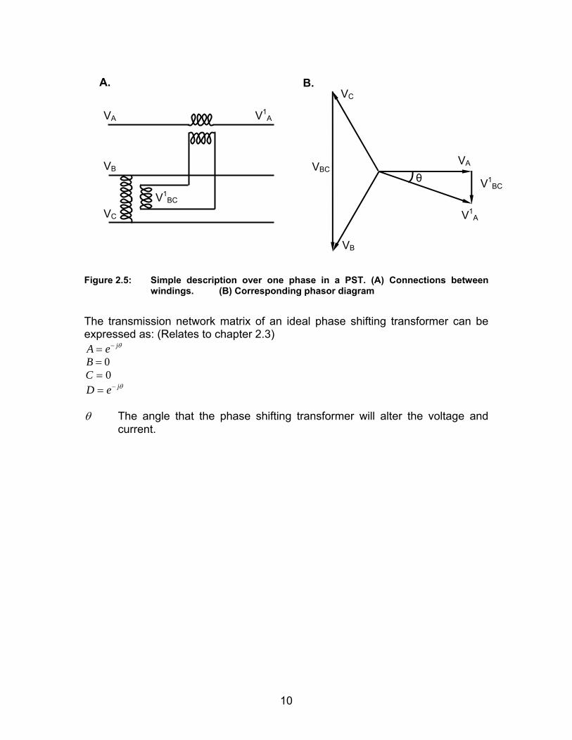
In an interconnected power system the bus voltage levels are kept fairly constant and the bus voltage is common for all circuits connected to the bus. The reactance, X , is a physical constant depending on the construction of the circuits. One way to regulate power flowing through a circuit is to reduce/increase the phase angle in the circuit. The principal of a PST is that it inserts voltage into one phase by energizing voltage from the other two phases in order to alter the phase angle and alter the voltage. Figure 2.5 describes the connections of a single phase in a PST, there are similar connections for the other two phases. There are different types of PST:s, Figure 2.5 describes one simplified type. All PST:s have on-load tap changers which enables stepwise regulation. By having many steps the power flow can be regulated gradually. The regulation can be in a positive angle,θ which increases the power flow. The regulation can also be in a negative angle, θ− which decreases the power flow. The PST can increase or decrease the power by altering the phase angle ( )θγ Δ+ in Equation 2.2. [2]

9

VA

V1A

VC

VB

VBC

V1BC

θ

A. B.

VA

VB

VC

V1A

V1BC

Figure 2.5: Simple description over one phase in a PST. (A) Connections between

windings. (B) Corresponding phasor diagram

The transmission network matrix of an ideal phase shifting transformer can be expressed as: (Relates to chapter 2.3)

θjeA −= 0=B 0=C

θjeD −= θ The angle that the phase shifting transformer will alter the voltage and

current.

10

3 Simulation program The simulation program is written in a Matlab M-file. This program builds on the transmission matrix theory (chapter 2.3). In order to determine the ABCD parameters for a circuit some basic data is needed: (see Equation 2.1)

1 The resistance of the circuit per phase and km. This is the “r” in the series impedance, . The program takes the resistive losses into account, see zFigure 2.3.

2 The inductance of the circuit per phase and km. This is the “x” in the series impedance, . z

3 The shunt capacitance of the circuit per phase and km. This is the “b” in the shunt admittance, y . The conductance “g” is assumed to be zero.

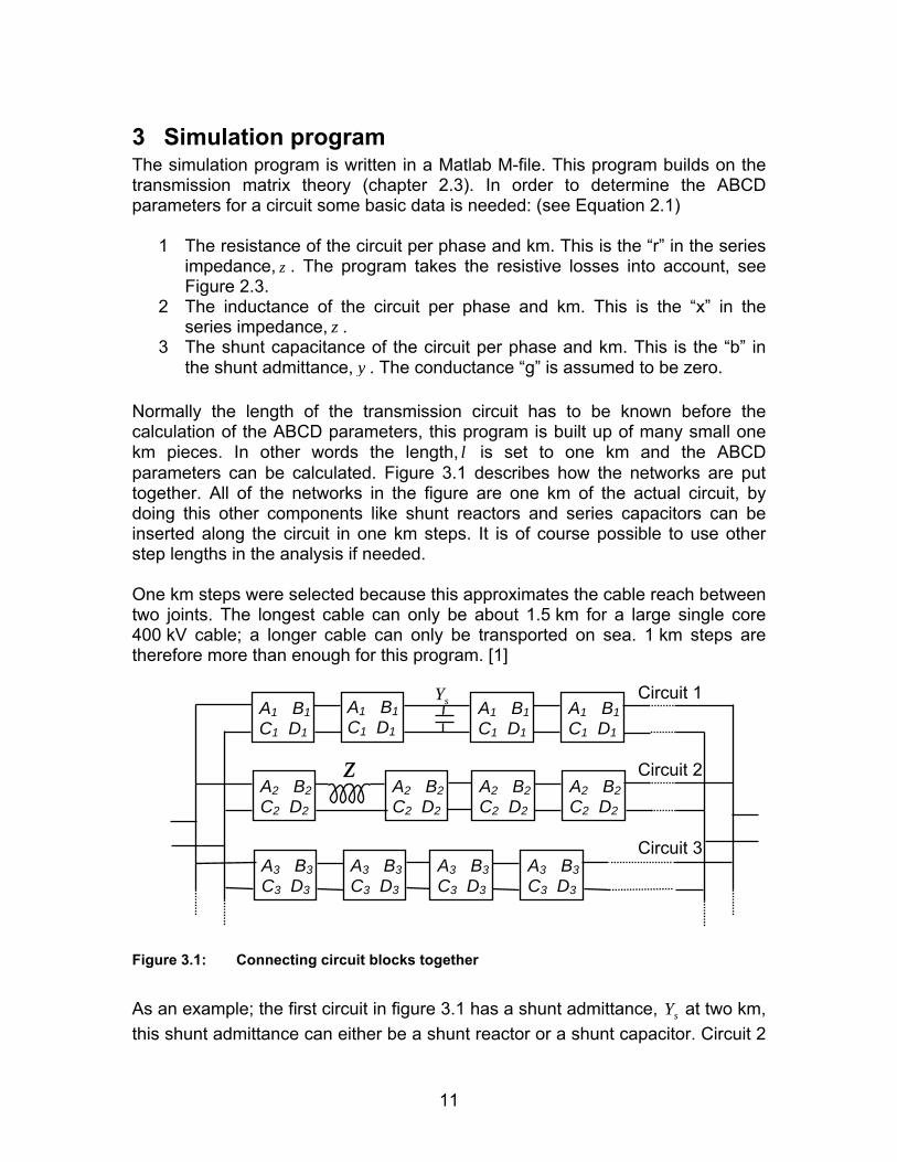
Normally the length of the transmission circuit has to be known before the calculation of the ABCD parameters, this program is built up of many small one km pieces. In other words the length, l is set to one km and the ABCD parameters can be calculated. Figure 3.1 describes how the networks are put together. All of the networks in the figure are one km of the actual circuit, by doing this other components like shunt reactors and series capacitors can be inserted along the circuit in one km steps. It is of course possible to use other step lengths in the analysis if needed. One km steps were selected because this approximates the cable reach between two joints. The longest cable can only be about 1.5 km for a large single core 400 kV cable; a longer cable can only be transported on sea. 1 km steps are therefore more than enough for this program. [1]

Figure 3.1: Connecting circuit blocks together

As an example; the first circuit in figure 3.1 has a shunt admittance, sY at two km, this shunt admittance can either be a shunt reactor or a shunt capacitor. Circuit 2

A1 B1C1 D1

A1 B1C1 D1

A1 B1C1 D1

A1 B1C1 D1

A2 B2C2 D2

A2 B2C2 D2

A2 B2C2 D2

A3 B3C3 D3

A3 B3C3 D3

A3 B3C3 D3

A2 B2C2 D2

sY

z

A3 B3C3 D3

Circuit 1

Circuit 2

Circuit 3

11

Zhas series impedance, at one km, this series impedance can either be a series reactor or a series capacitor. The program has a choice matrix which defines where all different series and shunt components are located, it also defines which circuit that is used i.e. A or A . ,B ,C ,D ,B ,C ,D1 1 1 1 2 2 2 2 The program iterates along the circuit and saves the accumulated network every km. When all circuits are calculated respectively, the next thing is to make a parallel connection of all circuits. This parallel connection starts with connecting circuit 1 and 2 into one new network, after this the new network and circuit 3 is connected and so on. The result when all circuits are connected is a final network, Atot,Btot,Ctot,Dtot, which represent the whole system between two nodes in one set of parameters. Now its time to calculate voltages and currents, the receiving end is normally used as a reference. The receiving end voltage, is set to be phase reference, then the load at the receiving end defines how large and with what phase angle the current, shall be. By using

RV

RI Equation 2.1 the sending end voltage, and current, can be calculated. The voltage and current at both the sending end and receiving end is now known. These currents are the total amount of currents through all circuits together. It is crucial to know the current going through every individual circuits; otherwise it would be impossible to calculate the voltages and currents at different points inside each circuit. By taking the network parameters for circuit 1 and solving the receiving end current when knowing the voltages and the sending end current,

SV

SI

equation 2.1 is used. The current in each circuit is derived i.e. the sending end voltage and current for circuit 1 is known, it is now possible to go back to the saved accumulated network and derive the voltage and current at every km in the circuit. The program only needs the voltages and currents to be able to calculate active power, reactive power, angle differences, power factors etc. The program displays the calculations in different diagrams; these diagrams are used in all cases later on.

12

4 Illustrative Cases The purpose of this chapter is to analyze some cases that will result when underground cables are installed in transmission networks consisting mainly of overhead lines. The first case consists of two overhead lines in parallel, it describes a common situation in transmission grids used today, overhead lines. The later cases illustrate cables in parallel with overhead lines and the problems that occur.

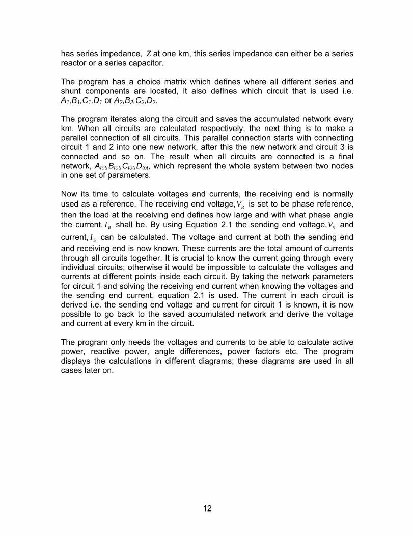
4.1 Case 1, two overhead lines in parallel To illustrate two overhead lines in parallel, theory of longer circuits is used. Circuit lengths are 200 km each and the nominal voltage is 400 kV. The reactance is for both of the circuits 0.3 Ω/km. The resistance, RLX , for circuit 1 and circuit 2 is 0.015 Ω/km and 0.03 Ω/km each. The shunt capacitance is 12 nF per phase and km. At the receiving end the load is 1500 MVA with a variable power factor. Figure 4.1 represents the two circuits.

1V 2V 3 Ω + 60j Ω 1500 MVA 6 Ω + 60j Ω

Figure 4.1: Representation of two overhead lines in parallel

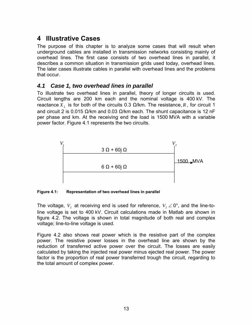
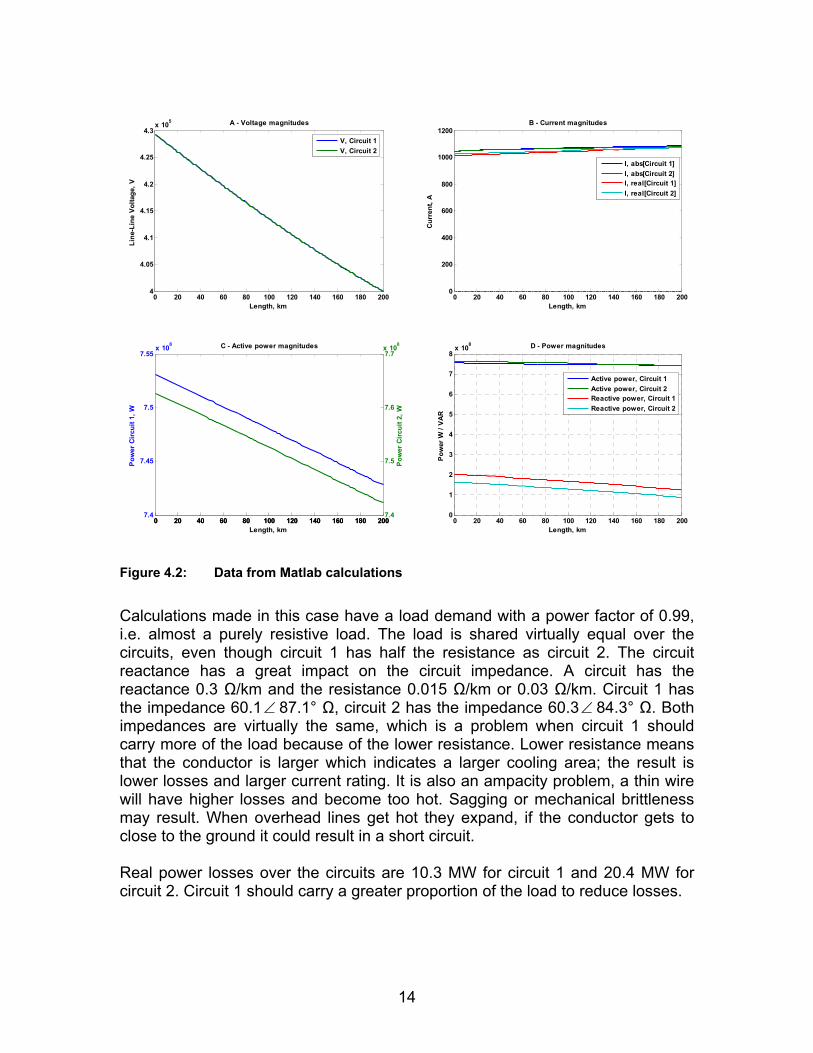
The voltage, at receiving end is used for reference, 2V 2V ∠ 0°, and the line-to-line voltage is set to 400 kV. Circuit calculations made in Matlab are shown in figure 4.2. The voltage is shown in total magnitude of both real and complex voltage; line-to-line voltage is used. Figure 4.2 also shows real power which is the resistive part of the complex power. The resistive power losses in the overhead line are shown by the reduction of transferred active power over the circuit. The losses are easily calculated by taking the injected real power minus ejected real power. The power factor is the proportion of real power transferred trough the circuit, regarding to the total amount of complex power.

13

0 20 40 60 80 100 120 140 160 180 2004

4.05

4.1

4.15

4.2

4.25

4.3x 105

Length, km

Line

-Lin

e Vo

ltage

, VA - Voltage magnitudes

V, Circuit 1V, Circuit 2

0 20 40 60 80 100 120 140 160 180 2000

200

400

600

800

1000

1200

Length, km

Cur

rent

, A

B - Current magnitudes

I, abs[Circuit 1]I, abs[Circuit 2]I, real[Circuit 1]I, real[Circuit 2]

0 20 40 60 80 100 120 140 160 180 2007.4

7.45

7.5

7.55x 108

Pow

er C

ircu

it 1,

W

Length, km

C - Active power magnitudes

0 20 40 60 80 100 120 140 160 180 2007.4

7.5

7.6

7.7x 108

Pow

er C

ircu

it 2,

W

0 20 40 60 80 100 120 140 160 180 2000

1

2

3

4

5

6

7

8x 108

Length, km

Pow

er W

/ V

AR

D - Power magnitudes

Active power, Circuit 1Active power, Circuit 2Reactive power, Circuit 1Reactive power, Circuit 2

Figure 4.2: Data from Matlab calculations

Calculations made in this case have a load demand with a power factor of 0.99, i.e. almost a purely resistive load. The load is shared virtually equal over the circuits, even though circuit 1 has half the resistance as circuit 2. The circuit reactance has a great impact on the circuit impedance. A circuit has the reactance 0.3 Ω/km and the resistance 0.015 Ω/km or 0.03 Ω/km. Circuit 1 has the impedance 60.1 87.1° Ω, circuit 2 has the impedance 60.3∠ 84.3° Ω. Both impedances are virtually the same, which is a problem when circuit 1 should carry more of the load because of the lower resistance. Lower resistance means that the conductor is larger which indicates a larger cooling area; the result is lower losses and larger current rating. It is also an ampacity problem, a thin wire will have higher losses and become too hot. Sagging or mechanical brittleness may result. When overhead lines get hot they expand, if the conductor gets to close to the ground it could result in a short circuit.

∠

Real power losses over the circuits are 10.3 MW for circuit 1 and 20.4 MW for circuit 2. Circuit 1 should carry a greater proportion of the load to reduce losses.

14

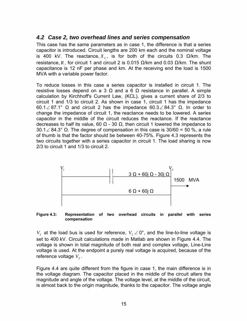
4.2 Case 2, two overhead lines and series compensation This case has the same parameters as in case 1, the difference is that a series capacitor is introduced. Circuit lengths are 200 km each and the nominal voltage is 400 kV. The reactance, , is for both of the circuits 0.3 Ω/km. The resistance,

LXR , for circuit 1 and circuit 2 is 0.015 Ω/km and 0.03 Ω/km. The shunt

capacitance is 12 nF per phase and km. At the receiving end the load is 1500 MVA with a variable power factor. To reduce losses in this case a series capacitor is installed in circuit 1. The resistive losses depend on a 3 Ω and a 6 Ω resistance in parallel. A simple calculation by Kirchhoff's Current Law, (KCL), gives a current share of 2/3 to circuit 1 and 1/3 to circuit 2. As shown in case 1, circuit 1 has the impedance 60.1∠ 87.1° Ω and circuit 2 has the impedance 60.3∠ 84.3° Ω. In order to change the impedance of circuit 1, the reactance needs to be lowered. A series capacitor in the middle of the circuit reduces the reactance. If the reactance decreases to half its value, 60 Ω - 30 Ω, then circuit 1 lowered the impedance to 30.1∠ 84.3° Ω. The degree of compensation in this case is 30/60 = 50 %, a rule of thumb is that the factor should be between 40-75%. Figure 4.3 represents the two circuits together with a series capacitor in circuit 1. The load sharing is now 2/3 to circuit 1 and 1/3 to circuit 2.

1V 2V 3 Ω + 60j Ω - 30j Ω 1500 MVA

6 Ω + 60j Ω

Figure 4.3: Representation of two overhead circuits in parallel with series

compensation

2V 2V ∠ at the load bus is used for reference, 0°, and the line-to-line voltage is

set to 400 kV. Circuit calculations made in Matlab are shown in Figure 4.4. The voltage is shown in total magnitude of both real and complex voltage, Line-Line voltage is used. At the endpoint a purely real voltage is acquired, because of the reference voltage . 2V Figure 4.4 are quite different from the figure in case 1, the main difference is in the voltage diagram. The capacitor placed in the middle of the circuit alters the magnitude and angle of the voltage. The voltage level, at the middle of the circuit, is almost back to the origin magnitude, thanks to the capacitor. The voltage angle

15

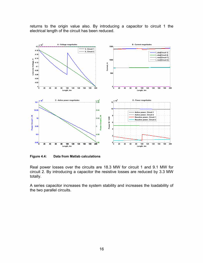
returns to the origin value also. By introducing a capacitor to circuit 1 the electrical length of the circuit has been reduced.

0 20 40 60 80 100 120 140 160 180 2004

4.02

4.04

4.06

4.08

4.1

4.12

4.14

4.16

4.18

4.2x 105

Length, km

Line

-Lin

e Vo

ltage

, V

A - Voltage magnitudes

V, Circuit 1V, Circuit 2

0 20 40 60 80 100 120 140 160 180 2000

500

1000

1500

Length, km

Curr

ent,

A

B - Current magnitudes

I, abs[Circuit 1]I, abs[Circuit 2]I, real[Circuit 1]I, real[Circuit 2]

0 20 40 60 80 100 120 140 160 180 2009.85

9.9

9.95

10

10.05

10.1x 108

Pow

er C

ircu

it 1,

W

Length, km

C - Active power magnitudes

0 20 40 60 80 100 120 140 160 180 2004.96

4.98

5

5.02

5.04

5.06x 108

Pow

er C

ircu

it 2,

W

0 20 40 60 80 100 120 140 160 180 2000

2

4

6

8

10

12x 108

Length, km

Pow

er W

/ V

AR

D - Power magnitudes

Active power, Circuit 1Active power, Circuit 2Reactive power, Circuit 1Reactive power, Circuit 2

Figure 4.4: Data from Matlab calculations

Real power losses over the circuits are 18.3 MW for circuit 1 and 9.1 MW for circuit 2. By introducing a capacitor the resistive losses are reduced by 3.3 MW totally. A series capacitor increases the system stability and increases the loadability of the two parallel circuits.

16

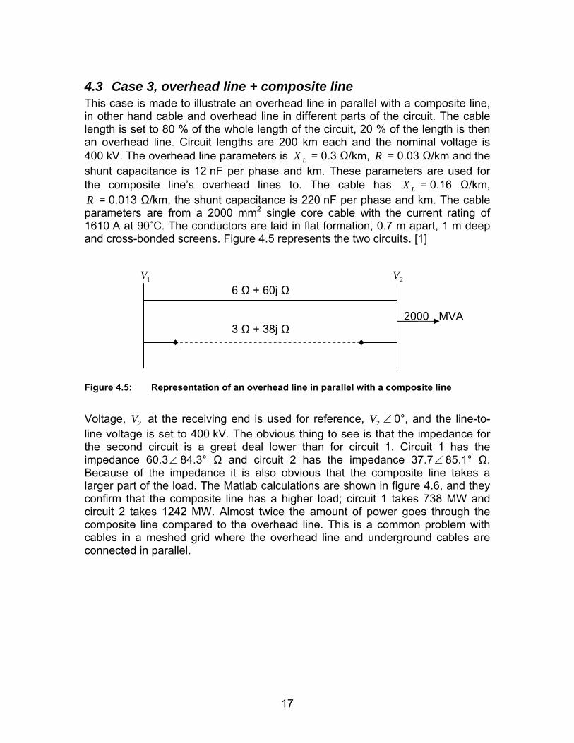
4.3 Case 3, overhead line + composite line This case is made to illustrate an overhead line in parallel with a composite line, in other hand cable and overhead line in different parts of the circuit. The cable length is set to 80 % of the whole length of the circuit, 20 % of the length is then an overhead line. Circuit lengths are 200 km each and the nominal voltage is 400 kV. The overhead line parameters is = 0.3 Ω/km, RLX = 0.03 Ω/km and the shunt capacitance is 12 nF per phase and km. These parameters are used for the composite line’s overhead lines to. The cable has = 0.16 Ω/km, LXR = 0.013 Ω/km, the shunt capacitance is 220 nF per phase and km. The cable parameters are from a 2000 mm2 single core cable with the current rating of 1610 A at 90˚C. The conductors are laid in flat formation, 0.7 m apart, 1 m deep and cross-bonded screens. Figure 4.5 represents the two circuits. [1]

1V 2V 6 Ω + 60j Ω 2000 MVA 3 Ω + 38j Ω

Figure 4.5: Representation of an overhead line in parallel with a composite line

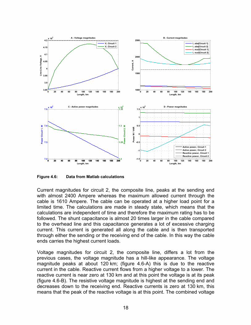
Voltage, at the receiving end is used for reference, 2V 2V ∠ 0°, and the line-to-line voltage is set to 400 kV. The obvious thing to see is that the impedance for the second circuit is a great deal lower than for circuit 1. Circuit 1 has the impedance 60.3∠ 84.3° Ω and circuit 2 has the impedance 37.7∠ 85.1° Ω. Because of the impedance it is also obvious that the composite line takes a larger part of the load. The Matlab calculations are shown in figure 4.6, and they confirm that the composite line has a higher load; circuit 1 takes 738 MW and circuit 2 takes 1242 MW. Almost twice the amount of power goes through the composite line compared to the overhead line. This is a common problem with cables in a meshed grid where the overhead line and underground cables are connected in parallel.

17

0 20 40 60 80 100 120 140 160 180 2003.85

3.9

3.95

4

4.05

4.1

4.15

4.2x 105

Length, km

Line

-Lin

e Vo

ltage

, VA - Voltage magnitudes

V, Circuit 1V, Circuit 2

0 20 40 60 80 100 120 140 160 180 2001000

1500

2000

2500

Length, km

Cur

rent

, A

B - Current magnitudes

I, abs[Circuit 1]I, abs[Circuit 2]I, real[Circuit 1]I, real[Circuit 2]

0 20 40 60 80 100 120 140 160 180 2007.2

7.3

7.4

7.5x 108

Pow

er C

ircu

it 1,

W

Length, km

C - Active power magnitudes

0 20 40 60 80 100 120 140 160 180 2001.2

1.25

1.3

1.35x 109

Pow

er C

ircu

it 2,

W

0 20 40 60 80 100 120 140 160 180 200-1.5

-1

-0.5

0

0.5

1

1.5x 109

Length, km

Pow

er W

/ V

AR

D - Power magnitudes

Active power, Circuit 1Active power, Circuit 2Reactive power, Circuit 1Reactive power, Circuit 2

Figure 4.6: Data from Matlab calculations

Current magnitudes for circuit 2, the composite line, peaks at the sending end with almost 2400 Ampere whereas the maximum allowed current through the cable is 1610 Ampere. The cable can be operated at a higher load point for a limited time. The calculations are made in steady state, which means that the calculations are independent of time and therefore the maximum rating has to be followed. The shunt capacitance is almost 20 times larger in the cable compared to the overhead line and this capacitance generates a lot of excessive charging current. This current is generated all along the cable and is then transported through either the sending or the receiving end of the cable. In this way the cable ends carries the highest current loads. Voltage magnitudes for circuit 2, the composite line, differs a lot from the previous cases, the voltage magnitude has a hill-like appearance. The voltage magnitude peaks at about 120 km; (figure 4.6-A) this is due to the reactive current in the cable. Reactive current flows from a higher voltage to a lower. The reactive current is near zero at 130 km and at this point the voltage is at its peak (figure 4.6-B). The resistive voltage magnitude is highest at the sending end and decreases down to the receiving end. Reactive currents is zero at 130 km, this means that the peak of the reactive voltage is at this point. The combined voltage

18

of the resistive and reactive is called complex voltage, this is the voltage shown in figure 4.6. This case illustrates the difficulties when combining overhead lines and cables. The next cases introduce series compensation in the circuits in order to handle some of the obstacles.

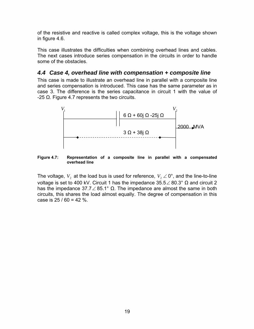
4.4 Case 4, overhead line with compensation + composite line This case is made to illustrate an overhead line in parallel with a composite line and series compensation is introduced. This case has the same parameter as in case 3. The difference is the series capacitance in circuit 1 with the value of -25 Ω. Figure 4.7 represents the two circuits.

1V 2V 6 Ω + 60j Ω -25j Ω 2000 MVA 3 Ω + 38j Ω

Figure 4.7: Representation of a composite line in parallel with a compensated

overhead line

The voltage, at the load bus is used for reference, 2V 2V ∠ 0°, and the line-to-line voltage is set to 400 kV. Circuit 1 has the impedance 35.5∠ 80.3° Ω and circuit 2 has the impedance 37.7 85.1° Ω. The impedance are almost the same in both circuits, this shares the load almost equally. The degree of compensation in this case is 25 / 60 = 42 %.

∠

19

0 20 40 60 80 100 120 140 160 180 2003.85

3.9

3.95

4

4.05

4.1

4.15

4.2

4.25x 105

Length, km

Line

-Lin

e Vo

ltage

, VA - Voltage magnitudes

V, Circuit 1V, Circuit 2

0 20 40 60 80 100 120 140 160 180 2001300

1400

1500

1600

1700

1800

1900

2000

2100

2200

Length, km

Cur

rent

, A

B - Current magnitudes

I, abs[Circuit 1]I, abs[Circuit 2]I, real[Circuit 1]I, real[Circuit 2]

0 20 40 60 80 100 120 140 160 180 2009.6

9.8

10

10.2x 108

Pow

er C

ircu

it 1,

W

Length, km

C - Active power magnitudes

0 20 40 60 80 100 120 140 160 180 2001

1.02

1.04

1.06x 109

Pow

er C

ircu

it 2,

W

0 20 40 60 80 100 120 140 160 180 200-1.5

-1

-0.5

0

0.5

1

1.5x 109

Length, km

Pow

er W

/ V

AR

D - Power magnitudes

Active power, Circuit 1Active power, Circuit 2Reactive power, Circuit 1Reactive power, Circuit 2

Figure 4.8: Data from Matlab calculations

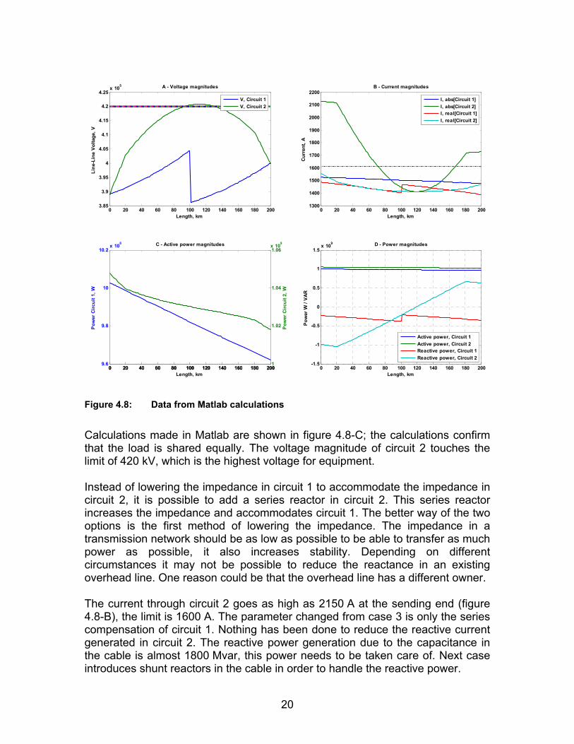
Calculations made in Matlab are shown in figure 4.8-C; the calculations confirm that the load is shared equally. The voltage magnitude of circuit 2 touches the limit of 420 kV, which is the highest voltage for equipment. Instead of lowering the impedance in circuit 1 to accommodate the impedance in circuit 2, it is possible to add a series reactor in circuit 2. This series reactor increases the impedance and accommodates circuit 1. The better way of the two options is the first method of lowering the impedance. The impedance in a transmission network should be as low as possible to be able to transfer as much power as possible, it also increases stability. Depending on different circumstances it may not be possible to reduce the reactance in an existing overhead line. One reason could be that the overhead line has a different owner. The current through circuit 2 goes as high as 2150 A at the sending end (figure 4.8-B), the limit is 1600 A. The parameter changed from case 3 is only the series compensation of circuit 1. Nothing has been done to reduce the reactive current generated in circuit 2. The reactive power generation due to the capacitance in the cable is almost 1800 Mvar, this power needs to be taken care of. Next case introduces shunt reactors in the cable in order to handle the reactive power.

20

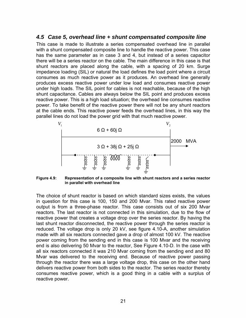
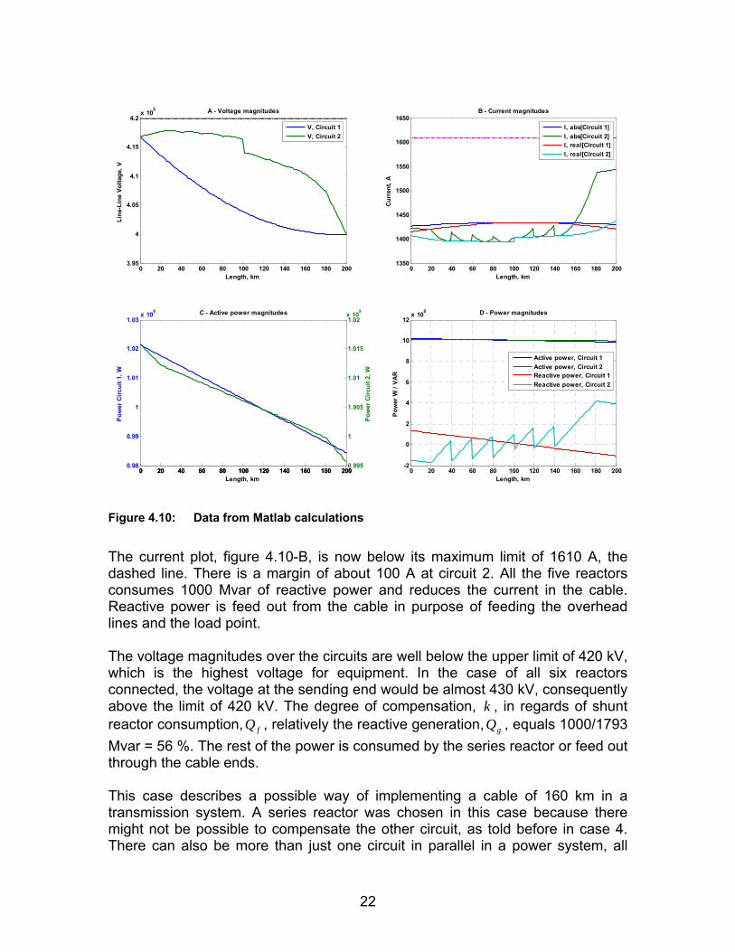
4.5 Case 5, overhead line + shunt compensated composite line This case is made to illustrate a series compensated overhead line in parallel with a shunt compensated composite line to handle the reactive power. This case has the same parameter as in case 3 and 4, but instead of a series capacitor there will be a series reactor on the cable. The main difference in this case is that shunt reactors are placed along the cable, with a spacing of 20 km. Surge impedance loading (SIL) or natural the load defines the load point where a circuit consumes as much reactive power as it produces. An overhead line generally produces excess reactive power under low load and consumes reactive power under high loads. The SIL point for cables is not reachable, because of the high shunt capacitance. Cables are always below the SIL point and produces excess reactive power. This is a high load situation; the overhead line consumes reactive power. To take benefit of the reactive power there will not be any shunt reactors at the cable ends. This reactive power feeds the overhead lines, in this way the parallel lines do not load the power grid with that much reactive power.

1V 2V 6 Ω + 60j Ω 2000 MVA 3 Ω + 38j Ω + 25j Ω

Figure 4.9: Representation of a composite line with shunt reactors and a series reactor

in parallel with overhead line

The choice of shunt reactor is based on which standard sizes exists, the values in question for this case is 100, 150 and 200 Mvar. This rated reactive power output is from a three-phase reactor. This case consists out of six 200 Mvar reactors. The last reactor is not connected in this simulation, due to the flow of reactive power that creates a voltage drop over the series reactor. By having the last shunt reactor disconnected, the reactive power through the series reactor is reduced. The voltage drop is only 20 kV, see figure 4.10-A, another simulation made with all six reactors connected gave a drop of almost 100 kV. The reactive power coming from the sending end in this case is 100 Mvar and the receiving end is also delivering 50 Mvar to the reactor, See Figure 4.10-D. In the case with all six reactors connected it was 210 Mvar coming from the sending end and 80 Mvar was delivered to the receiving end. Because of reactive power passing through the reactor there was a large voltage drop, this case on the other hand delivers reactive power from both sides to the reactor. The series reactor thereby consumes reactive power, which is a good thing in a cable with a surplus of reactive power.

21

0 20 40 60 80 100 120 140 160 180 2003.95

4

4.05

4.1

4.15

4.2x 105

Length, km

Line

-Lin

e Vo

ltage

, VA - Voltage magnitudes

V, Circuit 1V, Circuit 2

0 20 40 60 80 100 120 140 160 180 2001350

1400

1450

1500

1550

1600

1650

Length, km

Cur

rent

, A

B - Current magnitudes

I, abs[Circuit 1]I, abs[Circuit 2]I, real[Circuit 1]I, real[Circuit 2]

0 20 40 60 80 100 120 140 160 180 2000.98

0.99

1

1.01

1.02

1.03x 109

Pow

er C

ircu

it 1,

W

Length, km

C - Active power magnitudes

0 20 40 60 80 100 120 140 160 180 2000.995

1

1.005

1.01

1.015

1.02x 109

Pow

er C

ircu

it 2,

W

0 20 40 60 80 100 120 140 160 180 200-2

0

2

4

6

8

10

12x 108

Length, km

Pow

er W

/ V

AR

D - Power magnitudes

Active power, Circuit 1Active power, Circuit 2Reactive power, Circuit 1Reactive power, Circuit 2

Figure 4.10: Data from Matlab calculations

The current plot, figure 4.10-B, is now below its maximum limit of 1610 A, the dashed line. There is a margin of about 100 A at circuit 2. All the five reactors consumes 1000 Mvar of reactive power and reduces the current in the cable. Reactive power is feed out from the cable in purpose of feeding the overhead lines and the load point. The voltage magnitudes over the circuits are well below the upper limit of 420 kV, which is the highest voltage for equipment. In the case of all six reactors connected, the voltage at the sending end would be almost 430 kV, consequently above the limit of 420 kV. The degree of compensation, , in regards of shunt reactor consumption, , relatively the reactive generation, , equals 1000/1793 Mvar = 56 %. The rest of the power is consumed by the series reactor or feed out through the cable ends.

kfQ gQ

This case describes a possible way of implementing a cable of 160 km in a transmission system. A series reactor was chosen in this case because there might not be possible to compensate the other circuit, as told before in case 4. There can also be more than just one circuit in parallel in a power system, all

22

parallel circuits would have to be compensated. Later on in the Sydlänken case, there are four circuits in parallel. Compensation on the cable is bound to happen.

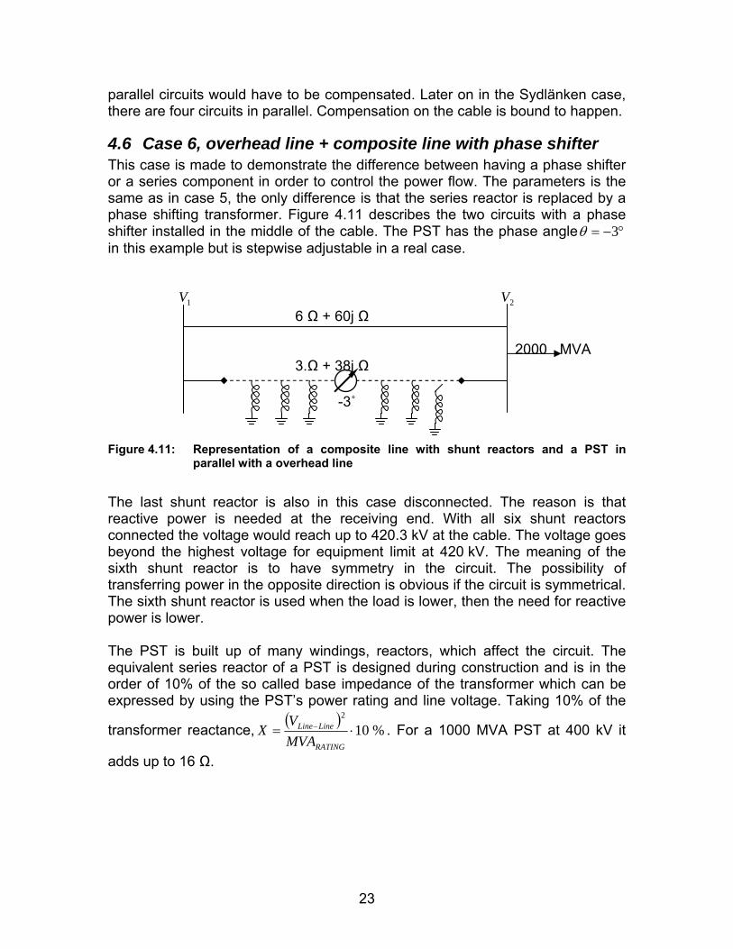
4.6 Case 6, overhead line + composite line with phase shifter This case is made to demonstrate the difference between having a phase shifter or a series component in order to control the power flow. The parameters is the same as in case 5, the only difference is that the series reactor is replaced by a phase shifting transformer. Figure 4.11 describes the two circuits with a phase shifter installed in the middle of the cable. The PST has the phase angle °−= 3θ in this example but is stepwise adjustable in a real case.

1V 2V 6 Ω + 60j Ω 2000 MVA 3.Ω + 38j Ω

-3˚

Figure 4.11: Representation of a composite line with shunt reactors and a PST in

parallel with a overhead line

The last shunt reactor is also in this case disconnected. The reason is that reactive power is needed at the receiving end. With all six shunt reactors connected the voltage would reach up to 420.3 kV at the cable. The voltage goes beyond the highest voltage for equipment limit at 420 kV. The meaning of the sixth shunt reactor is to have symmetry in the circuit. The possibility of transferring power in the opposite direction is obvious if the circuit is symmetrical. The sixth shunt reactor is used when the load is lower, then the need for reactive power is lower. The PST is built up of many windings, reactors, which affect the circuit. The equivalent series reactor of a PST is designed during construction and is in the order of 10% of the so called base impedance of the transformer which can be expressed by using the PST’s power rating and line voltage. Taking 10% of the

transformer reactance,( )

%102

⋅= −

RATING

LineLine

MVAV

X . For a 1000 MVA PST at 400 kV it

adds up to 16 Ω.

23

0 20 40 60 80 100 120 140 160 180 2003.95

4

4.05

4.1

4.15

4.2x 105

Length, km

Line

-Lin

e Vo

ltage

, VA - Voltage magnitudes

V, Circuit 1V, Circuit 2

0 20 40 60 80 100 120 140 160 180 2001400

1450

1500

1550

1600

1650

Length, km

Cur

rent

, A

B - Current magnitudes

I, abs[Circuit 1]I, abs[Circuit 2]I, real[Circuit 1]I, real[Circuit 2]

0 20 40 60 80 100 120 140 160 180 2000.98

1

1.02x 109

Pow

er C

ircu

it 1,

W

Length, km

C - Active power magnitudes

0 20 40 60 80 100 120 140 160 180 2000.98

1

1.02x 109

Pow

er C

ircu

it 2,

W

0 20 40 60 80 100 120 140 160 180 200-4

-2

0

2

4

6

8

10

12x 108

Length, km

Pow

er W

/ V

AR

D - Power magnitudes

Active power, Circuit 1Active power, Circuit 2Reactive power, Circuit 1Reactive power, Circuit 2

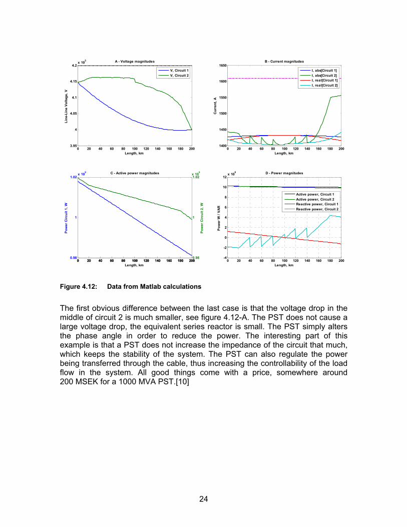
Figure 4.12: Data from Matlab calculations

The first obvious difference between the last case is that the voltage drop in the middle of circuit 2 is much smaller, see figure 4.12-A. The PST does not cause a large voltage drop, the equivalent series reactor is small. The PST simply alters the phase angle in order to reduce the power. The interesting part of this example is that a PST does not increase the impedance of the circuit that much, which keeps the stability of the system. The PST can also regulate the power being transferred through the cable, thus increasing the controllability of the load flow in the system. All good things come with a price, somewhere around 200 MSEK for a 1000 MVA PST.[10]

24

5 Transmission grid, Sydlänken, single core cable, 400kV

5.1 Background Sydlänken is a project that shall reinforce the power grid in the southern parts of Sweden, in the province Skåne. This project connects the Hallsberg substation to a new substation at Hörby, see Figure 5.1. One of the underlying reasons behind building this circuit is the blackout that occurred 23 September in 2003. The blackout affected the southern parts of Sweden and east Denmark. The entire grid below Hallsberg and Kinna was affected. A reinforcement circuit from Hallsberg down to Hörby was then suggested. Another reason for the Sydlänken project is to increase the import/export capability of power to Denmark, Poland and Germany. [11]

5.2 Sydlänken parameters The project has two main alternatives, an overhead line or an underground HVDC Light (High voltage direct current) cable. A HVDC Light alternative would also be a way of increasing and controlling the voltage in Skåne. Increasing the voltage in Skåne will ultimately result in a capacity increase of all the other circuits carrying power down to Skåne. The Swedish power grid is split up into different sections; the blue dashed line in Figure 5.1 is called section 4. This section can under normal conditions transfer as much as 4500 MW. Worth mentioning is that this section lies precisely south of the two nuclear power plants, Oskarshamn (east coast) and Ringhals (west coast). The plants can regulate voltage and reactive power which increases the power capabilities in section 4. There are not many large power plants south of this section in Sweden; therefore most of the power flowing down is consumed by various load points along the way. In other terms, the transfer capability down to Hörby is much less than 4500 MW, a high estimate is 3500 MW. Together with the new Sydlänken circuit, which shall carry 500 MW, it sums up to 4000 MW. The overhead line alternative must be able to carry 500 MW of power down to Hörby, this alternative does not increase the voltage. The HVDC Light alternative

Figure 5.1: Sydlänken, reinforces the soutern parts of Sweden.

400 kV 220 kV Sydlänken

25

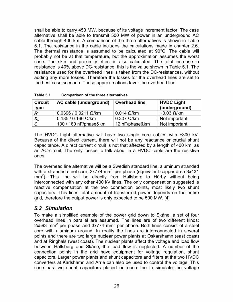
shall be able to carry 450 MW, because of its voltage increment factor. The case alternative shall be able to transmit 500 MW of power in an underground AC cable through 400 km. A comparison of the three alternatives is shown in Table 5.1. The resistance in the cable includes the calculations made in chapter 2.6. The thermal resistance is assumed to be calculated at 90°C. The cable will probably not be at that temperature, but the approximation assumes the worst case. The skin and proximity effect is also calculated. The total increase in resistance is 40% above DC-resistance, this is the value shown in Table 5.1. The resistance used for the overhead lines is taken from the DC-resistances, without adding any more losses. Therefore the losses for the overhead lines are set to the best case scenario. These approximations favor the overhead line. Table 5.1 Comparison of the three alternatives

Circuit type

AC cable (underground) Overhead line HVDC Light (underground)

0.0396 / 0.0211 Ω/km 0.014 Ω/km ~0.03 Ω/km R 0.185 / 0.166 Ω/km 0.307 Ω/km Not important XL130 / 180 nF/phase&km 12 nF/phase&km Not important C

The HVDC Light alternative will have two single core cables with ±300 kV. Because of the direct current, there will not be any reactance or crucial shunt capacitance. A direct current circuit is not that affected by a length of 400 km, as an AC-circuit. The only losses to talk about in a HVDC cable are the resistive ones. The overhead line alternative will be a Swedish standard line, aluminum stranded with a stranded steel core, 3x774 mm2 per phase (equivalent copper area 3x431 mm2). This line will be directly from Hallsberg to Hörby without being interconnected with any other 400 kV lines. The only compensation suggested is reactive compensation at the two connection points, most likely two shunt capacitors. This lines total amount of transferred power depends on the entire grid, therefore the output power is only expected to be 500 MW. [4]

5.3 Simulation To make a simplified example of the power grid down to Skåne, a set of four overhead lines in parallel are assumed. The lines are of two different kinds; 2x593 mm2 2 per phase and 3x774 mm per phase. Both lines consist of a steel core with aluminum around. In reality the lines are interconnected in several points and there are two large nuclear power plants at Oskarshamn (east coast) and at Ringhals (west coast). The nuclear plants affect the voltage and load flow between Hallsberg and Skåne, the load flow is neglected. A number of the connection points in the grid have equipment for voltage regulation, shunt capacitors. Larger power plants and shunt capacitors and filters at the two HVDC converters at Karlshamn and Arrie can also be used to control the voltage. This case has two shunt capacitors placed on each line to simulate the voltage

26

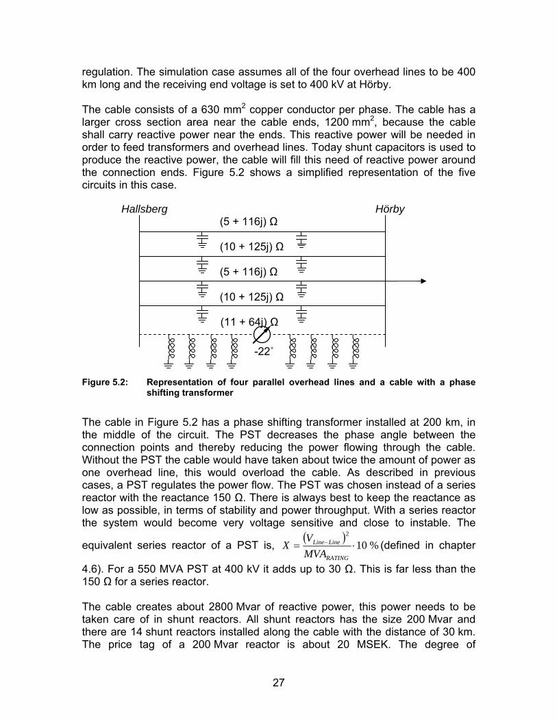
regulation. The simulation case assumes all of the four overhead lines to be 400 km long and the receiving end voltage is set to 400 kV at Hörby.

2The cable consists of a 630 mm copper conductor per phase. The cable has a larger cross section area near the cable ends, 1200 mm2, because the cable shall carry reactive power near the ends. This reactive power will be needed in order to feed transformers and overhead lines. Today shunt capacitors is used to produce the reactive power, the cable will fill this need of reactive power around the connection ends. Figure 5.2 shows a simplified representation of the five circuits in this case.

Hallsberg Hörby (5 + 116j) Ω (10 + 125j) Ω (5 + 116j) Ω (10 + 125j) Ω

(11 + 64j) Ω

-22˚

Figure 5.2: Representation of four parallel overhead lines and a cable with a phase shifting transformer

The cable in Figure 5.2 has a phase shifting transformer installed at 200 km, in the middle of the circuit. The PST decreases the phase angle between the connection points and thereby reducing the power flowing through the cable. Without the PST the cable would have taken about twice the amount of power as one overhead line, this would overload the cable. As described in previous cases, a PST regulates the power flow. The PST was chosen instead of a series reactor with the reactance 150 Ω. There is always best to keep the reactance as low as possible, in terms of stability and power throughput. With a series reactor the system would become very voltage sensitive and close to instable. The

equivalent series reactor of a PST is, ( )

%102

⋅= −

RATING

LineLine

MVAV

X (defined in chapter

4.6). For a 550 MVA PST at 400 kV it adds up to 30 Ω. This is far less than the 150 Ω for a series reactor. The cable creates about 2800 Mvar of reactive power, this power needs to be taken care of in shunt reactors. All shunt reactors has the size 200 Mvar and there are 14 shunt reactors installed along the cable with the distance of 30 km. The price tag of a 200 Mvar reactor is about 20 MSEK. The degree of

27

compensation, k , in regards of shunt reactor consumption, , relatively the reactive generation, , equals 2800/2800 Mvar = 100%. This seems like a lot, but this is needed in order to manage the energization of the cable. Energizing a circuit means that the receiving end is open, the receiving end current, , is then equal to zero. The receiving end is not connected and the cable must maintain a voltage below the highest voltage for equipment, which is 420 kV. Further harmonic studies are needed in order to establish that 100% compensation is a viable case. There could be resonance at this high compensation grade.

fQ

gQ

RI

0 50 100 150 200 250 300 350 4004

4.05

4.1

4.15

4.2x 10

5

Length, km

Line

-Lin

e Vo

ltage

, V

Voltage magnitudes along the cable, when open end

V, Zsa = 0 ΩV, Zsa = 32 Ω

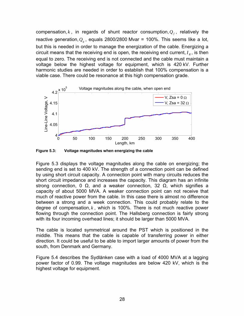
Figure 5.3: Voltage magnitudes when energizing the cable

Figure 5.3 displays the voltage magnitudes along the cable on energizing; the sending end is set to 400 kV. The strength of a connection point can be defined by using short circuit capacity. A connection point with many circuits reduces the short circuit impedance and increases the capacity. This diagram has an infinite strong connection, 0 Ω, and a weaker connection, 32 Ω, which signifies a capacity of about 5000 MVA. A weaker connection point can not receive that much of reactive power from the cable. In this case there is almost no difference between a strong and a week connection. This could probably relate to the degree of compensation, , which is 100%. There is not much reactive power flowing through the connection point. The Hallsberg connection is fairly strong with its four incoming overhead lines; it should be larger than 5000 MVA.

k

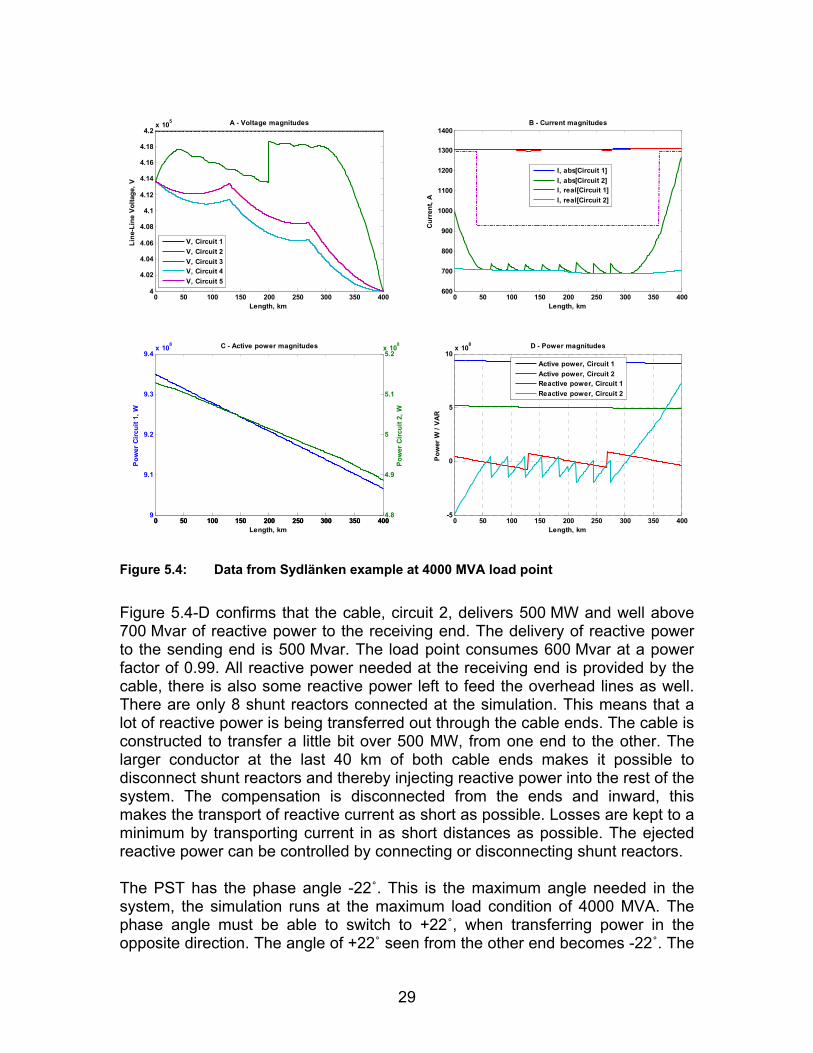
The cable is located symmetrical around the PST which is positioned in the middle. This means that the cable is capable of transferring power in either direction. It could be useful to be able to import larger amounts of power from the south, from Denmark and Germany. Figure 5.4 describes the Sydlänken case with a load of 4000 MVA at a lagging power factor of 0.99. The voltage magnitudes are below 420 kV, which is the highest voltage for equipment.

28

0 50 100 150 200 250 300 350 4004

4.02

4.04

4.06

4.08

4.1

4.12

4.14

4.16

4.18

4.2x 105

Length, km

Line

-Lin

e Vo

ltage

, VA - Voltage magnitudes

V, Circuit 1V, Circuit 2V, Circuit 3V, Circuit 4V, Circuit 5

0 50 100 150 200 250 300 350 400600

700

800

900

1000

1100

1200

1300

1400

Length, km

Cur

rent

, A

B - Current magnitudes

I, abs[Circuit 1]I, abs[Circuit 2]I, real[Circuit 1]I, real[Circuit 2]

0 50 100 150 200 250 300 350 4009

9.1

9.2

9.3

9.4x 108

Pow

er C

ircu

it 1,

W

Length, km

C - Active power magnitudes

0 50 100 150 200 250 300 350 4004.8

4.9

5

5.1

5.2x 108

Pow

er C

ircu

it 2,

W

0 50 100 150 200 250 300 350 400-5

0

5

10x 108

Length, km

Pow

er W

/ V

AR

D - Power magnitudes

Active power, Circuit 1Active power, Circuit 2Reactive power, Circuit 1Reactive power, Circuit 2

Figure 5.4: Data from Sydlänken example at 4000 MVA load point

Figure 5.4-D confirms that the cable, circuit 2, delivers 500 MW and well above 700 Mvar of reactive power to the receiving end. The delivery of reactive power to the sending end is 500 Mvar. The load point consumes 600 Mvar at a power factor of 0.99. All reactive power needed at the receiving end is provided by the cable, there is also some reactive power left to feed the overhead lines as well. There are only 8 shunt reactors connected at the simulation. This means that a lot of reactive power is being transferred out through the cable ends. The cable is constructed to transfer a little bit over 500 MW, from one end to the other. The larger conductor at the last 40 km of both cable ends makes it possible to disconnect shunt reactors and thereby injecting reactive power into the rest of the system. The compensation is disconnected from the ends and inward, this makes the transport of reactive current as short as possible. Losses are kept to a minimum by transporting current in as short distances as possible. The ejected reactive power can be controlled by connecting or disconnecting shunt reactors. The PST has the phase angle -22˚. This is the maximum angle needed in the system, the simulation runs at the maximum load condition of 4000 MVA. The phase angle must be able to switch to +22˚, when transferring power in the opposite direction. The angle of +22˚ seen from the other end becomes -22˚. The

29

PST in this case will have to manage angles from -25˚ to + 25˚ and have the rating of approximately 550 MVA, because there is always some reactive power flowing in either direction in the cable.

5.3.1 Losses The transfer losses in the new circuit are an important factor when deciding which alternative to use. A comparison of the three different types of circuits used in the simulation is shown in Table 5.2. Circuit 1 is the overhead line that is suggested in the Sydlänken project. Circuit 3 is the older type of overhead line used in Sweden. Circuit 1 has lower losses than the cable; this is of course due to the larger conductors (equals 1293 mm2 of copper). The losses in the grid are probably somewhere in between circuit 1 and circuit 3, because the load sharing is almost equal. Average losses for the overhead lines then

become %3.4829906

5.7%8293.1%906=

+⋅+⋅ . The losses per transferred watt is based

on real power only, the cable delivers more reactive power than real power in this example. Reactive power contributes to the losses; current of both active and reactive loads the conductor. More current means more losses. The losses in the shunt reactors are not taken into account. The losses are approximately 0.4 % for a shunt reactor, which means 0.8 MW per reactor. Table 5.2: Losses in the simulation

Resistive losses Circuit 1, New type 3x774 mm

Circuit 2, Cable

Circuit 3, Old type 3x593 mm2 2

28.2 22.1 47.3 Total losses (MW) 906 489 829 Transferred power (MW)

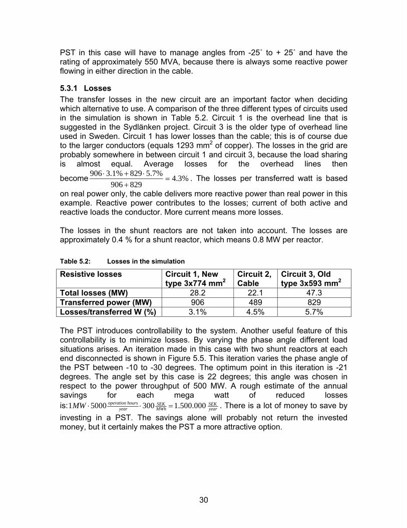
3.1% 4.5% 5.7% Losses/transferred W (%) The PST introduces controllability to the system. Another useful feature of this controllability is to minimize losses. By varying the phase angle different load situations arises. An iteration made in this case with two shunt reactors at each end disconnected is shown in Figure 5.5. This iteration varies the phase angle of the PST between -10 to -30 degrees. The optimum point in this iteration is -21 degrees. The angle set by this case is 22 degrees; this angle was chosen in respect to the power throughput of 500 MW. A rough estimate of the annual savings for each mega watt of reduced losses is: year

SEKMWhSEK

yearhoursoperationMW 000.500.130050001 =⋅⋅ . There is a lot of money to save by

investing in a PST. The savings alone will probably not return the invested money, but it certainly makes the PST a more attractive option.

30

-30 -28 -26 -24 -22 -20 -18 -16 -14 -12 -101.65

1.66

1.67

1.68

1.69

1.7

1.71

1.72x 10

8

Phase angle, degree

Tota

l los

ses,

Wat

t

Losses depending on PST:s phase angle

Figure 5.5: Losses in the complete circuit depending on the PST:s phase angle

5.4 Discussion The cable alternative is a feasible option in the range of 400 km from a steady state perspective. There are higher losses in the cable compared to the newer overhead line (circuit 1), but the overhead line was based on DC resistance. The choice of cable dimension could be larger, the 630 mm2 cable was chosen in respect to the transfer capabilities of 500 MW. The existing power grid used today is limited by the older overhead lines. The power transfer capabilities in new overhead lines are thereby far from fully utilized. A cable transfers to much power, which is the opposite of the new overhead lines. A PST could also be interesting for the new overhead line; it could increase the power throughput and thereby reduce losses. The cable has to be compensated with 14 shunt reactors; these reactors cost about 20 MSEK each. It sums up to 280 MSEK, probably less because of the quantity. The PST probably costs at least 100 MSEK, a 1000 MVA PST costs about 200 MSEK. A rough estimation could be that the compensation needed costs about 400 MSEK. This is quite a lot, but a PST is a good investment both in terms of extra controllability and loss reduction.

31

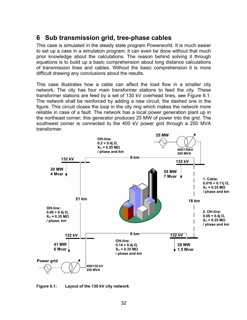
6 Sub transmission grid, tree-phase cables This case is simulated in the steady state program Powerworld. It is much easier to set up a case in a simulation program; it can even be done without that much prior knowledge about the calculations. The reason behind solving it through equations is to build up a basic comprehension about long distance calculations of transmission lines and cables. Without the basic comprehension it is more difficult drawing any conclusions about the results. This case illustrates how a cable can affect the load flow in a smaller city network. The city has four main transformer stations to feed the city. These transformer stations are feed by a set of 130 kV overhead lines, see Figure 6.1. The network shall be reinforced by adding a new circuit, the dashed one in the figure. This circuit closes the loop in the city ring which makes the network more reliable in case of a fault. The network has a local power generation plant up in the northeast corner; this generator produces 25 MW of power into the grid. The southwest corner is connected to the 400 kV power grid through a 250 MVA transformer.

132 kV

132 kV 132 kV

132 kV

21 km

6 km

8 km

18 km

25 MW

OH-line:0.14 + 0.4j Ω, XC = 0.35 MΩ / phase and km

OH-line: 0.08 + 0.4j Ω, XC = 0.35 MΩ / phase, km

OH-line:0.2 + 0.4j Ω, XC = 0.35 MΩ / phase and km

2. OH-line:0.08 + 0.4j Ω, XC = 0.35 MΩ / phase and km

1. Cable:0.018 + 0.11j Ω,XC = 0.35 MΩ / phase and km

Power grid

41 MW 6 Mvar

20 MW 4 Mvar 55 MW

7 Mvar

28 MW 1.5 Mvar

400/130 kV 250 MVA

400/130kV 200 MVA

Figure 6.1: Layout of the 130 kV city network

32

The new circuit can either be an overhead line or an underground cable. The overhead line parameters are 0.08 + 0.4j Ω with the shunt capacitance 350 kΩ per phase and km. The cable is suggested to be a 1000 mm2 with the parameters 0.018 + 0.11j Ω with the shunt capacitance 12.7 kΩ per phase and km. Let us assume that the generation plant up in the northeast corner has a fault. The northeast bus has to increase its load from the other two busses. The load flow over this system without the new circuit is shown in Appendix A. The southern line is this example is a 127 mm2 and has a maximum current throughput of about 2 A/ mm2, this line can then transmit about 60 MVA. The transmitted power on this link depends on which alternative that is used for the eastern link, Appendix B and Appendix C. The power through the southern link in the overhead line and cable alternative is 63 MVA and 73 MVA. Let us assume that the southern link can handle the load of 63 MVA. The cable has to be series compensated in some form. The simplest solution is to add a series reactor to the new eastern cable which reduces the power throughput. A PST can also be used but it is a bit more expensive. The series reactor of 9 Ω reduces the power through the southern to less than 60 MVA. A cable generates a lot of reactive power; this power is needed at the loads and transformers. The cable case feeds the 130 kV grid with reactive power, there is also 5 Mvar going back through the feeding 250 MVA transformer. The transformer consumes about 21 Mvar; this means that the city only has to buy 16 Mvar of reactive power from the 400 kV grid. In the overhead line alternative the city would have to buy 39 Mvar of reactive power. This is a significant difference and there could be money to save by having a cable that generates reactive power. Table 6.1: Power transmitted from the grid

Power transmitted from the grid

Before Cable with a series reactor

Overhead line

144.90 144.45 144.49 MW 41.53 15.76 38.68 Mvar

150.73 145.31 149.58 MVA Table 6.1 describes the difference between the three options. The overhead line alternative saves 410 kW while the cable saves 450 kW. As said before, the big difference lies in the amount of consumed reactive power where the cable alternative is the most favorable. There is a quite large difference in the total amount of complex power drawn from the grid, where the cable draws about 5 MVA less.

33

A real example is that the city of Lund in Sweden has two 130 kV cables connecting their three substations together, all of the substations has a primary connection from the grid. The cables works as backup in case of a fault and instead of shunt capacitors (provides reactive power).

34

7 Conclusion Cables has much lower impedance than overhead lines, this makes it necessary to investigate the power flow in some detail. Low impedance is better in terms of stability and power transfer, but the existing power grids used today consists of overhead lines. The cable may take on too much load in an interconnected power system. Some series compensation is always needed in order to balance the load sharing. The compensation can be a series capacitor or reactor in order to decrease or increase the impedance of the circuit. A better alternative is to use a PST as compensation, it can control and alter the power flow in real-time. The PST increases stability and can also be used for minimizing losses in a system. The shunt capacitance of a cable can be both an advantage and a disadvantage. Power systems need reactive power in order to feed lines, transformers and loads. The amount of reactive power needed differs a lot. An overhead line consumes reactive power at high loads, but at low loads it can produce excess reactive power. In a long cable circuit, i.e. Sydlänken, the cable produces to much reactive power; this reactive power has to be taken care of in shunt reactors. The amount of shunt compensation needed becomes expensive; this is the price for using a cable. The price should be set in relation to the fact that cables affect the surroundings less and the magnetic fields are greatly reduced. In a smaller network, i.e. the 130 kV example, a cable can be a good way of decreasing the amount of reactive power needed. The smaller grid don not need to buy reactive power from the power gird. Decreasing the reactive power also decreases the complex power drawn from the power grid.

8 Future work This thesis introduces the idea of a longer cable in an interconnected power system. This is not a complete solution, further calculations have to be made in order to have a complete due able option, calculations like stability, short-circuit, etc.

35

9 References [1] ABB, XLPE cable systems – user’s guide, Brochure issued by: ABB

Power Technologies AB, High Voltage Cables, SE-371 23 Karlskrona [2] B.M. Weedy and B.J Cory, 1998, Electric power systems, fourth edition [3] Danielsson Magnus, Svenska Kraftnät [4] Fingrid, kraftledningsprojekt - Genom luften eller i jorden, http://www.fingrid.fi/attachments/svenska/publikationer/GenomLuften.pdf

(070121) [5] Svenska kraftnät, 2006, Pilot study – Sydlänken, http://www.svk.se/upload/4563/SvK_Forstudie_060926_webb.pdf

(070121) [6] IEC, 1985, Chapter 601: Generation, transmission and distribution of

electricity – general [7] IEC, 1987, Chapter 604: Generation, Transmission and distribution of

electricity – general, [8] IEC 60287, Electric cables – Calculation of the current ratings [9] IEEE, George J Anders, 1997, Rating of electric power cables [10] Lindahl Sture, 2007, IEA Lunds Tekniska Högskola, tutoring [11] Svenska Kraftnät, 2003, Elavbrottet 23 september 2003 – händelser och

åtgärder, http://www.svk.se/upload/3592/Rapport_avbrott_20030923_for_webb.pdf

(070121)

36

[12] Thorburn Stefan, 2007, ABB Corporate research, tutoring [13] Turan Gönen, 1988, Electric power transmission system engineering:

analysis and design, [14] Walker Mark, 1982, Aluminum Electrical Conductor Handbook, Second

edition

37

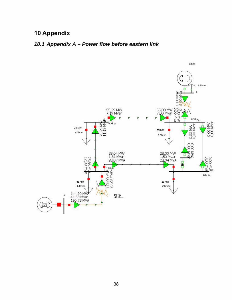
10 Appendix

10.1 Appendix A – Power flow before eastern link

38

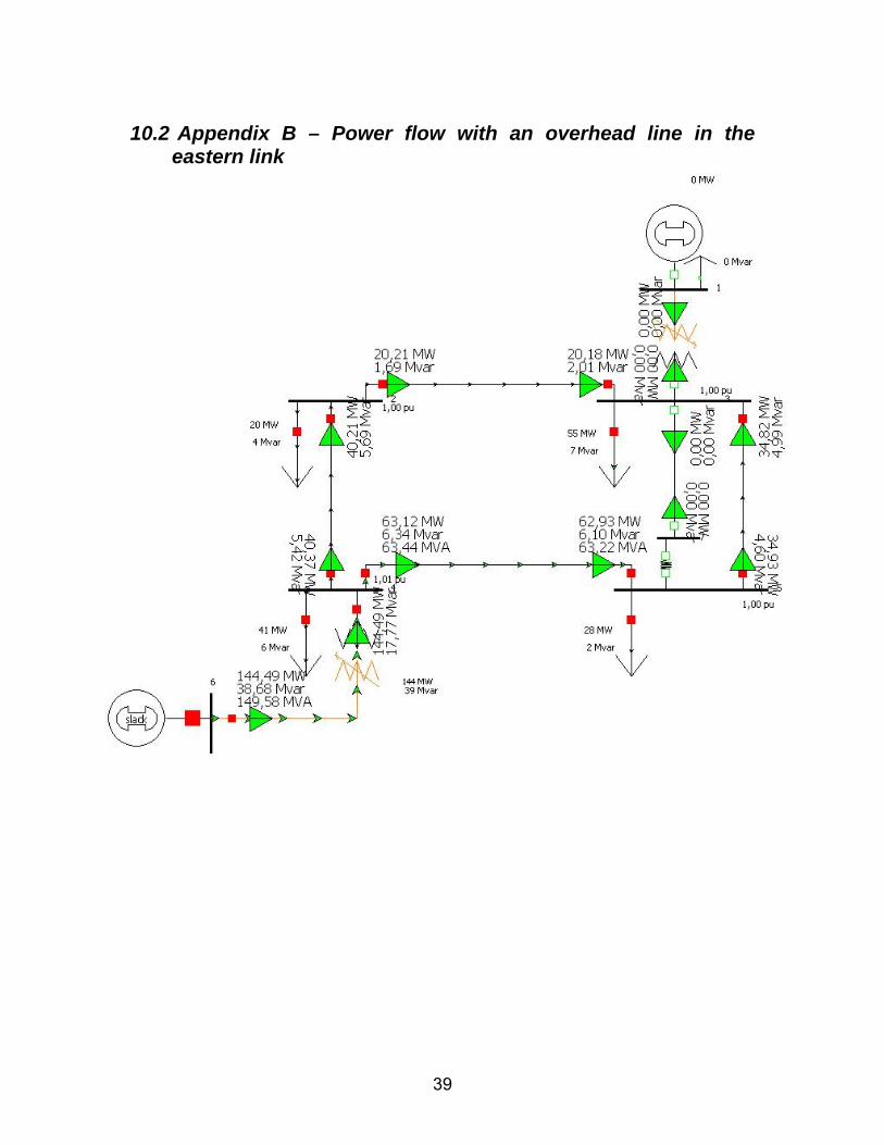
10.2 Appendix B – Power flow with an overhead line in the eastern link

39

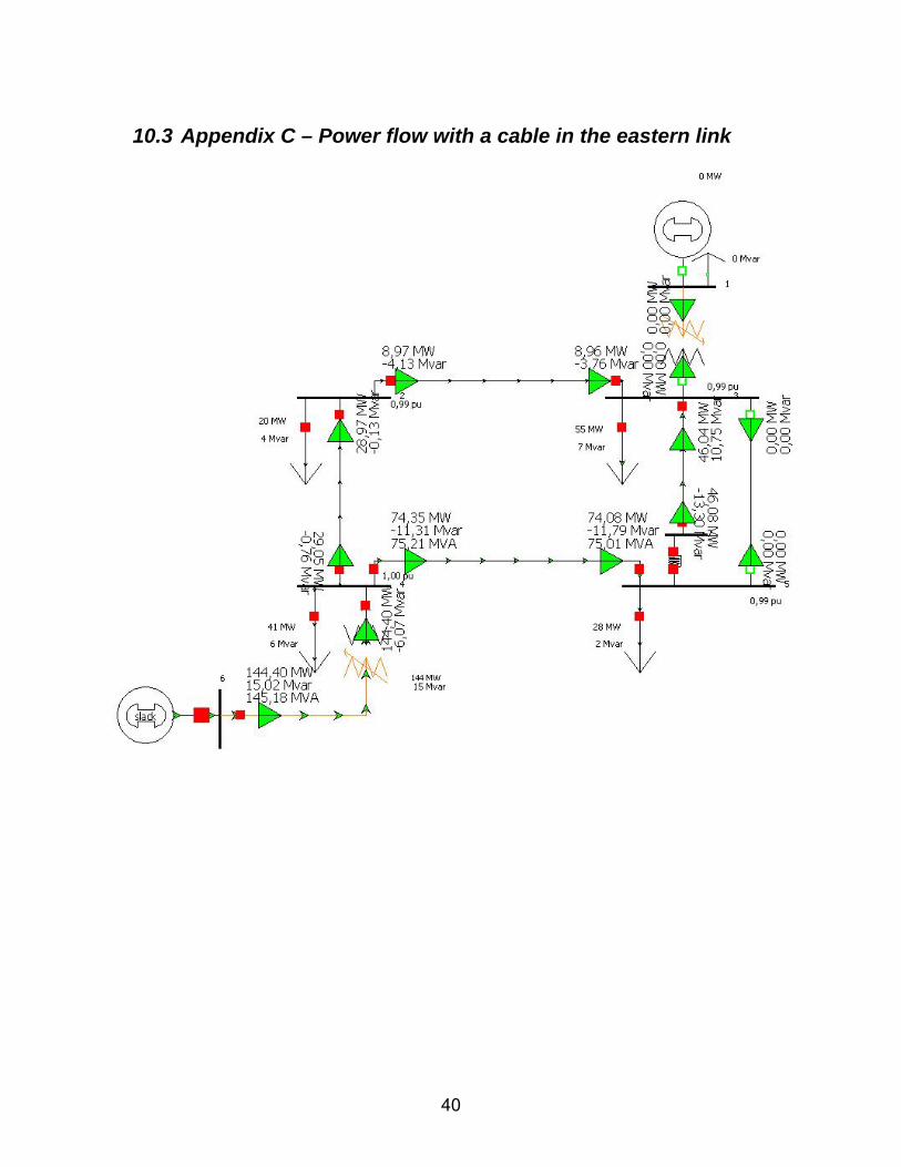
10.3 Appendix C – Power flow with a cable in the eastern link

40