Embed Size (px)
Citation preview

January 2013
Do not remove this if sending to pagerunnerr Page Title
UK Aviation Forecasts

The Department for Transport has actively considered the needs of blind and partially sighted people in accessing this document. The text will be made available in full on the Department’s website. The text may be freely downloaded and translated by individuals or organisations for conversion into other accessible formats. If you have other needs in this regard please contact the Department.
Department for Transport Great Minster House 33 Horseferry Road London SW1P 4DR Telephone 0300 330 3000 Website www.gov.uk/dft email enquiries [email protected]
© Crown copyright 2013
Copyright in the typographical arrangement rests with the Crown.
You may re-use this information (not including logos or third-party material) free of charge in any format or medium, under the terms of the Open Government Licence. To view this licence, visit www.nationalarchives.gov.uk/doc/open-government-licence/ or write to the Information Policy Team, The National Archives, Kew, London TW9 4DU, or e-mail: [email protected].
Where we have identified any third-party copyright information you will need to obtain permission from the copyright holders concerned.

Contents Executive summary ............................................................................................ 1
Introduction ..................................................................................................... 1 Key drivers of aviation demand....................................................................... 2 Approach to forecasting national demand ...................................................... 3 Approach to allocating passengers to airports ................................................ 4 National demand forecasts ............................................................................. 6 Airport level forecasts ..................................................................................... 8 Carbon emissions ........................................................................................... 9 Further information ......................................................................................... 9
1. Introduction ............................................................................................... 10 Nature and purpose of forecasts................................................................... 10 Document structure ...................................................................................... 11
2. DfT aviation forecasting............................................................................. 12 Overview....................................................................................................... 12 National Air Passenger Demand Model ........................................................ 15 National Air Passenger Allocation Model ...................................................... 21 Fleet Mix Model (FMM)................................................................................. 33 CO2 Emissions Model ................................................................................... 34
3. Input assumptions ..................................................................................... 37 Introduction ................................................................................................... 37 Assumptions driving passenger demand ...................................................... 37 Changes to relationships between passenger demand and its drivers ......... 44 Treatment of uncertainty ............................................................................... 47 Local growth adjustments ............................................................................. 49 Surface access to airports ............................................................................ 51 Freight........................................................................................................... 55 Airport capacities .......................................................................................... 56 Overseas hubs.............................................................................................. 58 Changing aircraft technology ........................................................................ 59 Calculating UK aviation CO2 emissions ........................................................ 61
4. Unconstrained passenger forecasts.......................................................... 66 Introduction (what is an unconstrained forecast?) ........................................ 66 Unconstrained passenger forecasts ............................................................. 66
5. Constrained passenger and aircraft forecasts........................................... 68 Introduction (what is a constrained forecast?) .............................................. 68 Passenger forecasts ..................................................................................... 68 ATM forecasts............................................................................................... 82
6. CO2 emissions forecasts ........................................................................... 84 Nature and purpose of forecasts................................................................... 84 Context of aviation greenhouse gas emissions............................................. 86 CO2 forecasts ............................................................................................... 88 Fuel efficiency............................................................................................... 90

7. Sensitivity tests ......................................................................................... 93 Approach ...................................................................................................... 93 Economic growth .......................................................................................... 93 Oil prices....................................................................................................... 95 Air fares ........................................................................................................ 96 Market maturity ............................................................................................. 97 Overview....................................................................................................... 99
8. Comparison with DfT 2011 forecasts ...................................................... 100 Introduction ................................................................................................. 100 Changes to methodology............................................................................ 101 Input variables ............................................................................................ 103 Unconstrained air passengers .................................................................... 105 Constrained passengers............................................................................. 107 Constrained ATMs ...................................................................................... 108 Airport use .................................................................................................. 108 CO2 emissions ............................................................................................ 110
9. Model performance ................................................................................. 111 Performance of the model over recent years .............................................. 111 Validation of airport, route and ATM forecasts............................................ 112
Annex A: Econometric models in the National Air Passenger Demand Model122 Data sources............................................................................................... 123 Econometric methods ................................................................................. 123 Technical Peer Review ............................................................................... 124 Econometric models used in the NAPDM................................................... 124 Long run air fare and income elasticities .................................................... 131 Implementation of market maturity in NAPDM............................................ 134
Annex B: Model validation results .................................................................. 138
Annex C: Key input variables ......................................................................... 145
Annex D Passenger forecasts (unconstrained) .............................................. 149
Annex E Passenger forecasts (constrained) .................................................. 156
Annex F: ATM forecasts (constrained) ........................................................... 167
Annex G: CO2 emission forecasts (constrained) ............................................ 171
Annex H: Glossary ......................................................................................... 177

Executive summary
Key findings
This report sets out forecasts of passenger numbers, air transport movements and aviation carbon emissions at UK airports.
Demand for air travel is forecast to increase within the range of 1% - 3% a year up to 2050, compared to historical growth rates of 5% a year over the last 40 years. The slowdown in growth rates in the future reflects the anticipation of market maturity across different passenger markets and a projected end to the long-term decline in average fares seen in the last two decades.
The central forecast, taking into account the impact of capacity constraints, is for passenger numbers at UK airports to increase from 219 million passengers in 2011 to 315 million in 2030 and 445 million by 2050. This is an increase of 225 million passengers over the next 40 years compared to an increase of 185 million since 1970.
The central forecasts of passenger numbers have been reduced by around 7% in 2030 from levels last forecast by the DfT in August 2011. Primarily this reflects revisions to the Office of Budget Responsibility's (OBR) forecasts for the UK economy and the Department of Energy and Climate Change's (DECC) projections of oil prices.
The major South East airports are forecast to be full by 2030. However, there is a range around this projection and they could be full as soon as 2025 or as late as 2040. Heathrow remains full across all the demand cases considered.
CO2 emissions from flights departing the UK are forecast to increase from 33.3 MtCO2 in 2011 to 47 MtCO2 within the range 35 – 52MtCO2 by 2050.
Introduction
1. This document sets out the Department for Transport (DfT) 2013 forecasts for aviation. The primary purpose of these forecasts is to inform long-term strategic aviation policy. For example, they support ongoing work on the development of the Government's sustainable framework for UK aviation (Aviation Policy Framework), the work of other Government departments and those working independently in the aviation sector.
1

2. The forecasts are presented as ranges to reflect the inherent uncertainty in forecasting to 2050. The range has been informed by evidence on the potential variability around the economic inputs expected to drive future air passenger growth. The range also allows for past relationships between economic inputs and aviation activity to change at different rates into the future.
Key drivers of aviation demand
3. The first step in forecasting future growth is to establish the historic relationships between demand and underlying economic variables. DfT analysis and assessments by external researchers have highlighted the two key drivers of this long-term growth in aviation demand shown in Figure 1: a long-term growth in incomes (which includes projected population growth) and a long-term decline in the real cost of air fares.1 Forecasts then use projections of these key drivers to predict future aviation demand at a national level. The UK economy and incomes are projected to return to long-term growth rates. However, it is expected that the decline in air fares will draw to a close as the opportunities for airlines to cut operating costs reduce and as the sector meets the increasing costs of its carbon dioxide (CO2) emissions.
Figure 1: Key drivers explaining historic air passenger demand growth
100
150
200
250
300
350
400
1984 1988 1992 1996 2000 2004 2008 2012
To
tal t
erm
ina
l pa
ss
en
ge
r in
de
x (
19
84
= 1
00
)
Contribution of decliningair fares
Contribution of risingeconomic activity
1 For example, Graham (2000) Demand for leisure air travel and limits to growth, Journal of Air Transport Management 6, 2000, 109-118 and Dargay and Hanley (2001) The determinants of demand for international air travel to and from the UK.
2

Approach to forecasting national demand
4. Table 1 summarises the range of sources used to project the key drivers of demand. As Table 1 shows, external and independent sources are used wherever possible. However, there is inevitably significant uncertainty about how these drivers will evolve, especially over the longer term. In order to capture this uncertainty a range of demand scenarios has been adopted (as outlined in Box 1).
Table 1: Key inputs to the national forecasts
Key driver Component Source
UK GDP and consumption Office of Budget Responsibility
Foreign GDP IMF & Enerdata
Income
Imports and exports Office of Budget Responsibility (OBR)
Fuel costs DECC (oil price) & DfT (fuel efficiency)
Non-fuel costs DfT projection
Air Passenger Duty (APD) Current HMRC published rates
Fares
Carbon costs DECC (carbon price) & DfT (carbon efficiency)
5. It is anticipated that the aviation market will "mature" - becoming progressively less responsive to changes in its key drivers. For example, growth in domestic air travel has slowed as it has to some of the European markets first served by the low cost carriers.
6. These forecasts adopt a series of judgment-based assumptions to reflect different levels of market maturity. The central assumption has the effect of reducing forecast demand by around 7% in 2030 and 21% in 2050 relative to a projection assuming no market maturity.
3

Box 1: Uncertainty in the national forecast
Variations in five key input variables are combined to produce high and low demand scenarios.
GDP: a key change from the approach to uncertainty used in DfT's August 2011 forecasts is the adoption of the OBR’s own assessment of the uncertainty in their GDP forecasts. DfT forecasts use the OBR's 20% and 80% confidence intervals around their central forecast until 2017. By 2015 this amounts to a range of +/- 2% compared to the central case GDP growth for that year. In the longer term the OBR's low and high productivity GDP cases are adopted.
Oil and carbon prices: DECC’s low and high scenarios are used to define the forecast range. By 2030 this means that oil prices are around 40% higher in the high demand case and 40% lower in the low demand case. Market maturity: the extent of market maturity can be strengthened or weakened in the model. In the high scenario market maturity assumptions are lowered – this increases demand by around 4% in 2030, relative to the central case. In the low demand case stronger market maturity is assumed – this decreases demand by around 10% in 2030 relative to the central case.
Behaviour change: the low demand case assumes that demand from business passengers is reduced by 10% as the use and impact on travel of video conferencing increases. The high demand case assumes an additional 5% growth in business passengers reflecting evidence that new communications technology could be a complement to traditional face-to-face meetings.2
GDP Growth uncertainty
Source: OBR Economic and Fiscal Outlook Dec 2012
OBR 20% to 80% confidence interval used in latest forecast
Previous +/- 0.25% per annum assumed in August 2011 forecasts
Approach to allocating passengers to airports
7. A passenger to airport allocation model is used to distribute the forecast of national passenger demand between 31 of the largest airports in the UK. Interviews of air passengers by the Civil Aviation Authority (CAA) are used to understand origins, destinations and travel purposes of
2 Committee on Climate Change Meeting the UK aviation target – options for reducing emissions to 2050 (2009).
4

passengers at UK airports. The model then predicts the airport choices of these passengers based on a statistical analysis of past decisions. The model can also then be used to incorporate the future impacts of capacity constraints at airports. Box 2 describes in stylised form the process followed by the airport choice model.
8. The approach outlined in Box 2 allows the UK aviation system to be modelled as a whole, explicitly taking into account the interactions between different airports. The model first produces "unconstrained" passenger forecasts. Unconstrained forecasts exclude the impacts of any runways or terminals reaching capacity, equivalent to assuming that all airports can expand by as much as they need to meet forecast national demand. The model then takes into account the effect of capacity limitations at airports, restricting the throughputs of passengers and aircraft movements to actual airport capacities in order to produce the "constrained" forecasts.
Box 2: How are passengers allocated to airports?
1. A passenger is more likely to use an airport that costs relatively less in terms of both time and money to reach than an airport that is more difficult to access.
2. Passengers prefer to use an airport that has more regular servicesto one that has less frequent services. This is intuitive as a more regular service increases the chance of finding a service at the desired time and reduces the risk from a missed connection. This relationship is modelled in additional detail. More passengers may lead to airlines offering either bigger aircraft or more frequent services. In the latter case, more passengers will in turn be attracted and cycles of increasing passengers and frequencies develop.
3. When the number of passengers choosing an airport exceeds the capacity at that airport, the model increases the cost of using that airport. This has two effects:- some passengers will choose an alternative airport; and- other passengers will choose not to fly.In both cases the demand will drop back to capacity at the congested airport. The model will iteratively increase the costs at all congested airports until no airport exceeds its input capacity.
Research has repeatedly found that there have been two key drivers of passenger choice of airport :
- the costs of travelling to airports; and,- the frequency of services offered at airports.
The relative importance of cost and frequency and other lesser factors and combined with a model to capture the impact of capacity constraints. This process works on a detailed geographic level and is outlined more fully below.
At the personal level passengers often take account of fares in their choice of airport. But at an aggregate level, and over the year, the differences in fares tend to average out to the extent that research rarely finds them a statistically significant determinant of airport choice.
Surface
access costs
Airport
choice
Frequency
of service
Capacity
constraints
5

National demand forecasts
Unconstrained forecasts
9. The unconstrained forecasts represent underlying estimates of demand in the absence of airport capacity constraints. Passengers are predicted to grow in the range of 1-3% a year over the period between 2010 and 2050. This is significantly lower than the growth of 5% a year seen over the past 40 years. This demonstrates an assumed gradual maturing of the aviation market and an end to the long-term decline in air fares seen over the previous two decades. In the central case this means that passenger numbers rise from 219 million passengers in 2011, reaching 320 million passengers by 2030 and 480 million by 2050. Figure 2 shows the new forecast of million passengers per annum (mppa) alongside the previous forecast made in 2011.
10. The new unconstrained forecast implies that, in the absence of capacity constraints, the growth in the number of international trips made per UK resident would fall from a long run average of around 4% a year, to just over 2% a year in the high demand case, 1.5% a year in the central demand case and just over 0.5% a year in the low demand case.
Figure 2: National unconstrained forecasts, million passengers per annum (mppa)
6

Constrained forecasts
11. The constrained forecasts, that assume no new runways are built in the UK, are lower than unconstrained forecasts by around 5 million passengers in 2030 and by around 35 million in 2050 in the central demand case. This means that passenger numbers are forecast to rise from 219 million passengers in 2011, reaching 315 million passengers by 2030 and 445 million by 2050 in the central case.
12. Overall the latest central forecast is lower than the DfT's previous 2030 forecast made in August 2011 by around 20 million passengers in (and 90 million from the 2009 forecast) and 25 million passengers in 2050 below the previous forecast. These changes and the effect of the recession on recent forecasts are discussed in more detail in Box 3.
13. In Figure 3 the high demand forecast is not shown beyond 2040. As all of the major airports are forecast to reach capacity, it is not possible to extend the forecast further. The 2011 forecasts shown alongside the new forecast the high growth case also ended at a similar time.3
Figure 3: National constrained forecasts, million passengers per annum (mppa)
3 However, in the 2011 published report the high growth forecast was extended beyond the point the model would run. Passenger numbers were extrapolated for each airport. The reason for this “off-model” extension was to estimate aviation carbon emissions in the high demand case, required at the time for the Government response to the Committee on Climate Change.
7

Airport level forecasts
14. In the central forecast, the five largest South East airports are forecast to be full by 2030. However, the high and low demand scenarios underline the uncertainty around this conclusion. With the range of demand used they could be full as soon as 2025 (the high case) or take until 2040 (the low case). Heathrow had effectively reached capacity in 2011 and it is forecast to remain at capacity in all scenarios.
15. In the high and central demand cases, a number of other airports are expected to reach capacity over the forecast period including Birmingham, Bristol, East Midlands and Manchester.
Box 3: Changes to the forecasts since August 2011
Overall the central unconstrained forecast is around 7% lower in 2030 compared to the DfT's August 2011 forecast. This is broadly similar to the drop in constrained forecasts.
The figure below shows the proportion of this total change that is attributable to each of the different input assumptions that have been updated.
2012 outturn passengers
Exchange rates
Carbon prices
Oil prices Foreign GDPUK GDP and
consumptionFleet
efficiency
-80%
-70%
-60%
-50%
-40%
-30%
-20%
-10%
0%
10%
Ch
an
ge
in p
ax
as
a p
erc
en
tag
e o
f to
tal c
ha
ng
e
2030 2050
Revisions to the OBR's projections of UK GDP and consumer expenditure account for the more than 60% of the total change in the forecast. Additionally, DECC's updated oil price projections and a revised approach to incorporating fleet efficiency improvements each account for around 10% of the overall decline in forecast passenger numbers.
This latest reduction of 25 million in the unconstrained terminal passenger central forecast for 2030 is considerably less than the 26% drop (120 million passengers) between the forecasts published in January 2009 and those in 2011. Between the DfT forecasts of 2009 and 2011, broadly comparable constrained scenarios saw a drop of 17% (70 million) compared to 7% (20 million) between 2011 and 2013.
8

9
Carbon emissions
16. The constrained passenger forecasts lead to a central prediction of CO2 emissions4 from aircraft departing UK airports growing from 33.3 million tonnes of carbon dioxide (MtCO2) in 2010 to 43.5 MtCO2 by 2030. The range around this forecast is 39.7 - 48.2 MtCO2. By 2050, UK aviation CO2 emissions are forecast to be 47.0 MtCO2, with a range around the forecast of 34.7 – 52.1MtCO2.
17. Post 2030, the growth in aviation CO2 emissions is forecast to slow as the effects of market maturity and airport capacity constraints causes a reduction in the rate of growth of activity at UK airports. Improvements in aircraft fuel efficiency are expected to continue beyond 2030 and, in the central and high forecasts, a small amount of biofuels is expected to penetrate the aircraft fleet as kerosene and carbon allowance prices increase. These projections also assume that the aviation sector pays a price for its emissions in line with DECC's projections of traded carbon prices.
Further information
18. The main document and its data annexes describe these forecasts and their methodology in more detail. Online supplementary tables also provide that information and some additional detail in accessible formats.
19. Requests for specific further information about the forecasts in this document can be made through:
4 Defined here as from all international and domestic flights departing UK airports.

1. Introduction
1.1 This document sets out the Department for Transport (DfT) 2013 forecasts for air passengers, aircraft movements and CO2 emissions at UK airports. The forecasts cover all years from the present to 2050. They are the eleventh set of forecasts produced by the Department since 1984 and supersede the last set of forecasts published in August 2011.5
1.2 The forecasts serve a number of purposes:
they take a view on a range of expected passenger demand and aircraft movements to inform potential aviation policies including their associated environmental assessments;
they provide estimates for the expected range of aviation greenhouse gas emissions which are used by the UK government in international negotiations; and
they are also used by other Government departments and those working independently within the aviation sector.
Nature and purpose of forecasts
1.3 The primary purpose of the passenger forecasts is to inform long term, strategic aviation policy. It is important to recognise that in making any prediction about the future there is inherent uncertainty and aviation demand is no exception. Low, central and high forecasts are presented in order to acknowledge this uncertainty in the forecasting process and present a range of possible outcomes reflecting alternative views of how key drivers of aviation demand may evolve over time.
1.4 More weight is placed on the role of these forecasts in informing long-term strategic policy than in providing detailed forecasts at each individual airport. For both continuity with previous publications and transparency of the forecasting methodology, airport level forecasts are included in this document. But the uncertainty reflected by the range at the national level is compounded at the level of the individual airport. At the airport level DfT forecasts may also differ from local airport forecasts. The latter may be produced for different purposes and may be informed by specific commercial and local information.
5 UK Aviation Forecasts, August 2011, http://assets.dft.gov.uk/publications/uk-aviation-forecasts-2011/uk-aviation-forecasts.pdf.
10

1.5 It should be noted that while the Department aims to accurately reflect existing planning restrictions on the expansion of airports, the forecasts should not in themselves be considered a cap on the development of individual airports. In some circumstances the airport specific forecasts could be used, in conjunction with additional relevant information, to inform local planning decisions.
1.6 Unrounded forecasts are generally presented in this document. This is primarily to give transparency to modelling outputs. The use of unrounded figures does not reflect the underlying level of certainty around individual results.
Document structure
1.7 The rest of this report is laid out in the following way:
Chapter 2 describes the models and methodology used by the DfT in producing these forecasts;
Chapter 3 sets out the input assumptions used in these forecasts;
Chapter 4 describes the composition of the range of forecasts unconstrained by any limits on UK airport capacity;
Chapter 5 describes the range of forecasts where demand is constrained to making best use of current airport capacity;
Chapter 6 presents the forecasts of CO2 emissions associated with the range of demand forecast;
Chapter 7 reports a number of sensitivity tests carried out to vary key input assumptions;
Chapter 8 compares this new forecast with the previous forecasts published by the Department in August 2011; and
Chapter 9 gives details on the performance of the underlying models in replicating 'actual' UK aviation activity.
1.8 A series of annexes describe some of the more technical aspects of the forecasting process in greater detail and give a more detailed breakdown of the results than is possible in the main part of the report. The data annexes are supplemented by electronic versions of the data tables which appear in this document.
11

2. DfT aviation forecasting
Overview
2.1 This section describes the methodology and assumptions used to produce forecasts of UK air passengers and air transport movements (ATMs). The forecasting framework described in this chapter was independently peer reviewed in 2010-11. This review concluded that the model was fit for the purpose of providing the forecast estimates required for policy development.6
2.2 The main stages of the Department's Aviation Model are shown in overview in Box 2.1 with the inputs, processes and outputs laid out in more detail in Figure 2.1.
Box 2.1 - Overview of the model
National Air Passenger Demand ModelUnconstrained
1. NAPDM forecasts national air travel demand at an aggregated level
2. NAPAM splits the national demand to form airport level forecasts of passengers and air transport movements (ATMs) on either an unconstrained or constrained basis
National Air Passenger Allocation ModelUnconstrained
National Air Passenger Allocation Model
Constrained
The passenger forecasts are generated in two steps: the National Air Passenger Demand Model (NAPDM) and the National Air Passenger Allocation Model (NAPAM)
Fleet Mix Model
6 Letter from NERA Economic consulting to DfT, July 2011 at: https://www.gov.uk/government/uploads/system/uploads/attachment_data/file/4505/peer-review-letter.pdf.
3. NAPAM ATM outputs are used in aircraft and emissions models
CO2 Emissions Model
12

Terminal passengers and air transport movements
2.3 The model forecasts the number of passengers passing through UK airports ('terminal passengers') each year. This covers UK and foreign residents travelling to, from or within the UK and those mainly foreign passengers passing through the UK and transferring at UK hubs. As part of the process to account for the impacts of airport capacity on passenger demand, the number of ATMs is also forecast.
2.4 The primary units of the forecasts are terminal passengers and ATMs. The Civil Aviation Authority (CAA) records the number of passengers, and the number of aircraft take-offs and landings, at UK airports each year.
2.5 The CAA further defines an ATM as a landing or take-off of an aircraft engaged on the transport of passengers, cargo or mail on commercial terms (excluding 'air taxi' movements, and empty positioning flights). As it does not include non-commercial movements, it also excludes private, aero-club, and military movements.
2.6 The CAA defines a 'terminal passenger' as a person joining or leaving an aircraft at a reporting airport, as part of ATM. This includes passengers 'interlining' (transferring between connecting services), but excludes those ’transiting' (arriving and departing on the same aircraft without entering the terminal) at a reporting UK airport.
2.7 The number of terminal passengers is related to, but not the same as, the number of trips by air to and from the UK. For example, a passenger making:
a direct, one way trip from the UK to an overseas destination would count as one terminal passenger;
a domestic, direct, one way trip would count as two terminal passengers (departing from an airport and arriving at an airport) ;
a one way trip from the UK to an overseas destination, via a UK connection (or transfer) would count as three terminal passengers; and,
a one way trip between two overseas countries via a connection in the UK would count as two terminal passengers.
2.8 A round trip would involve double the terminal passengers of a one-way trip. The full definitions of terminal passengers and air transport movements are available on the CAA website.7 A more detailed methodology statement can also be found in Annex A.
7 www.caa.co.uk/docs/80/airport_data/2006Annual/Foreward.pdf.
13

Figure 2.1: UK aviation forecasting framework
ConsumerSpending
GDP
carbon allowance prices
National Air Passenger
DemandModel
National AirPassenger
Allocation Model
UnconstrainedPassenger
Demand
Exchange rates
Trade
Market Maturity
Air PassengerDuty rates
Oil Prices
Fuel CostsNon Fuel
Costs
Carbon Charge
Air Fares
Airport capacities
Road/Rail costs
New aircraft bytype
Aircraft retirementages
Fuel efficiency ofnew aircraft
ATMs by route & size band
Shadow CostsAirport level passenger forecasts*
Fleet MixModel
Fuel efficiency offleet
ATMs by route & aircraft type
Route distances
Infrastructurecosts
Transport UserBenefits Model
CO2
ForecastingModel
CO2 emissions
Net benefits ofpotential policy
measures
Local demographic forecasts (DfT NTEM)
* these can be on a constrained or unconstrained basis
data input
model
intermediate output
final output
Key
14

National Air Passenger Demand Model
2.9 The National Air Passenger Demand Model (NAPDM) is used to forecast the number of UK air passengers up to 2050 assuming no UK airport capacity constraints. It does this by combining a set of time-series econometric models of past UK air travel demand with projections of key driving variables and assumptions about how the relationship between UK air travel and its key drivers will change into the future.
2.10 This analysis, along with independent academic research,8 highlights that historically there have been two key drivers of the long-term increases seen in aviation demand:
the long-term rise in incomes and economic activity9
the long-term decline in air fares.
2.11 The exact contribution of each varies by market segment, but, by way of illustration, Figure 2.2 shows a broad breakdown of the contributions of the two main drivers to overall passenger numbers in the UK (with population incorporated into the income driver).
Figure 2.2: Key drivers of overall air passenger demand
100
150
200
250
300
350
400
1984 1988 1992 1996 2000 2004 2008 2012
To
tal t
erm
ina
l pa
ss
en
ge
r in
de
x (
19
84
= 1
00
)
Contribution of decliningair fares
Contribution of risingeconomic activity
8 For example, Graham (2000), Demand for leisure air travel and limits to growth, Journal of Air Transport Management 6, 2000, 109-118 or Dargay and Hanley (2001), The determinants of demand for international air travel to and from the UK. 9 The rise in population projected in Office of National Statistics (ONS) forecasts is included in the forecast through the input forecasts of income and economic activity produced by the Office for Budget Responsibility (OBR) which in turn take account of population as an input.
15

Markets
2.12 The market for passenger air travel through UK airports can be split into separate sub-markets reflecting different trends, strength of driving forces and availability of data. Even before conducting statistical economic analysis, it might be expected that the demand for leisure trips would be driven by consumer spending, and to some extent affected by air fares. On the other hand, travel for business purposes might be expected to be driven by total GDP and international trade, and less affected by air fares at the aggregate national level. Similarly, it might be expected that the strength of the causal factors will vary between global regions, reflecting a range of factors including each region’s stage of economic development, the maturity of the air travel market to and from the UK and the availability of alternative modes of travel.
2.13 The market for passenger air travel is therefore split according to:
the global region the passenger is travelling to or from (see Figure 2.3);
whether the passenger is a UK or overseas resident;
the passenger's journey purpose (leisure or business);
whether the passenger has an international or domestic destination; and,
whether the passenger is passing through the UK making an international to international connection at a UK airport (as part of a journey between two other nations).
Figure 2.3: Global regions used in the National Air Passenger Demand
16
2.14 Overall, this gives nineteen market sectors for which separate econometric models are estimated and used to forecast demand. Annex A gives more technical detail on the econometric models underlying NAPDM.
Responsiveness of demand (elasticity)
2.15 Table 2.1 summarises the estimated long run elasticities of air passengers with respect to income and fares that have been used in producing the updated forecasts.10 These elasticities are derived from the 19 separate econometric models of air market sectors. The econometric models seek to statistically explain the historic relationship between the changes in the number of air passengers and changes in economic variables. The statistical relationships that best explain the behaviour are examined sector by sector. The historic data used covers the period 1984-2008. After 2008 NAPDM performance is controlled to actual passenger outturns up to 2011. The equations derived are then applied to projections of the explanatory variables to produce national level forecasts for each market sector.
2.16 Table 2.1 shows that income (which includes measures of population growth) is a strong driver in the domestic and UK markets, with the estimated income elasticity of demand ranging from 1.2 to 1.7. This falls to 1.0 for the foreign markets, and 0.5 for the international to international interliners market. The overall average income elasticity is strong at 1.3. Air fare elasticities are more variable. A strong price elasticity of -0.7 is used for the UK leisure sector, while a slightly lower value of -0.6 is used for the foreign leisure market. The fare elasticity for the domestic market is lower still at -0.5, although this elasticity combines the relatively price elastic (-0.7) domestic leisure sector, with the more price inelastic (-0.3) domestic business sector. Lower air fare elasticities of -0.2 are used for both the UK and foreign business markets.
10 The elasticity of demand with respect to another variable shows the percentage change in demand that would result from a 1% change in the other variable.
17

Table 2.1: Long run price and income elasticities of UK terminal passenger demand
Elasticity of demand with respect to
Sector Share of passenger demand in base
Income Air fares
UK Business 8% 1.2 -0.2
UK Leisure 45% 1.4 -0.7
Foreign Business 7% 1.0 -0.2
Foreign Leisure 14% 1.0 -0.6
International to international interliners
10% 0.5 -0.7
Domestic 15% 1.7 -0.5
Overall 100% 1.3 -0.6
Notes:
Income variable depends on sector.
Price and income elasticities are point estimates.
Results are elasticity of terminal passengers to income or fares.
2.17 The resulting overall air fare elasticity is -0.6. Air fares are often only a relatively small proportion of the overall journey cost: duration of stay, costs of getting to the airport, convenience and many other factors influence choice. It is intuitive that fare responsiveness is some way below unity, given that passengers may also have options beyond not travelling in their response to an increase in fare. For example, passengers might also reduce the cost of their trip by travelling to a less expensive destination, or by using a less expensive class of travel or airline. This overall fare elasticity is also in keeping with the findings for other modes that UK transport demand is price inelastic (i.e. has a price elasticity below -1). Box 2.2 explains that the elasticities presented in Table 2.1 are broadly consistent with other relevant published studies.
18

Box 2.2: National aviation demand price and income elasticities comparisons
In assessing the results of the econometric modelling, the price and income elasticities have been compared with those found in the literature. In choosing elasticities for comparison, it is essential to focus on studies which are relevant to the UK national passenger demand. For example, it would not be accurate to compare a national level price elasticity to that of a sub-national market, or an individual airline. As shown by CAA (2005), price effects at the sub-national level could be stronger, reflecting greater substitution possibilities, but substitution between routes or airlines would not affect the total market size. Also, comparisons with markets in other countries or regions of the world are complicated by their different population distribution, geography and transport systems, and market structures. A literature review revealed that while there is a large number of studies of aviation price and income elasticities, relatively few are relevant to UK national demand. Key studies which are directly comparable are Graham (2000),1 Dargay & Hanley (2001),2 CAA (2005)3 and Dargay, Menaz & Cairns (2006).4 None of these studies covers all the market sectors modelled and used for forecasting, but where they coincide they find price elasticities broadly comparable to those presented in this report.
The price elasticity of UK leisure travel is found to be -0.6 by Dargay & Hanley; in the range of -0.7 to -0.8 (outbound) by the CAA; and, -1.0 for short haul and 0.4 for long haul by Dargay. Menaz & Cairns could not find significant fare effects for UK business travel, while Dargay & Hanley found a small price effect of -0.3, slightly above the elasticity underpinning the updated forecast of -0.2. Dargay and Hanley also estimated a price elasticity of -0.3 for the foreign business and leisure markets, which is close to the elasticities of -0.2 and -0.6 used for these sectors in these updated forecasts.
The income elasticity of UK leisure travel is found to be 2.0 by Graham, 1.5-1.8 (outbound) by CAA, 1.1 by Dargay & Hanley, and 1.0 for short haul and 2.9 for long haul by Dargay, Menaz & Cairns. These results match well with the elasticity underpinning the updated forecasts of 1.4. UK business travel's income (trade) elasticity is found to be 1.5 by Dargay & Hanley, and 3.5 for short haul and 0.2 for long haul flights by Dargay, Menaz & Cairns. The domestic income elasticity (1.2) used reporting the updated forecasts therefore lies comfortably within this range. Only Dargay and Hanly (1.8), estimated income elasticities for the foreign leisure sector, rather higher than the elasticity used here of 1.0. 1 Graham (2000) Demand for leisure air travel and limits to growth, Journal of Air Transport Management 6, 2000, 109-118 2 Dargay & Hanley (2001) The Determinants of demand for international air travel to and from the UK 3 CAA (2005) Demand for outbound leisure air travel and its key drivers 4 Dargay, Menaz and Cairns (2006) Public attitudes towards aviation and climate change.
19

2.18 In 2011 an independent peer review reported on the econometric methods used to derive income and price elasticities and the work set out in more detail in Annex A. It concluded that it was "a difficult exercise competently implemented, with a satisfactory level of external input to check and add to the work's quality".11
Modelling market maturity
2.19 The term 'market maturity' is often used to refer to the process by which the demand for a product becomes less responsive to its key drivers through time. Air travel demand has shown very strong growth for several decades and while it would seem reasonable to start from the premise that the drivers of demand in the past will continue to drive demand in the future, this can only be the starting point. Any exercise to forecast the future must also consider how the relationships observed in the past might change in the future and whether any additional drivers might become important.
2.20 For example, as with most markets, one might expect there to be some form of product cycle in aviation, with rapid early demand growth giving way to slower growth in later years. Various possible explanations for this phenomenon are suggested in the literature. One explanation, specific to the market for leisure air travel, is that as the frequency of overseas trips increases, the time available for additional trips diminishes. This reduces the likelihood over time that the response to additional income will be an increase in demand for more leisure travel.
2.21 In 2010 the Department commissioned a detailed review of the available evidence on market maturity and other factors potentially affecting the relationship between air travel demand and its key drivers from the University of Westminster.12 Although it was not possible to uncover quantified evidence of how the response to key drivers changes over time, the review did recommend that a set of judgments about the date from which market maturity will take effect and the scale of the impact on the way passenger demand responds to changes in its key drivers be included in the forecast.
2.22 As a result, a range of assumptions about maturity are applied to the econometric forecasts in the NAPDM prior to the allocation of passenger demand to UK airports. Overall these assumptions act to reduce demand by between 4% and 14% in 2030 and between 11% and 36% in 2050. More information about these assumptions is given in the next chapter, with further discussion of the issue included in Annex B of UK Aviation
11 Report by NERA Economic Consulting https://www.gov.uk/government/uploads/system/uploads/attachment_data/file/4508/peer-review-econometrics.pdf. 12 University of Westminster, 2010 DfT Air Transport – Market Maturity - Summary Report, available here: http://assets.dft.gov.uk/publications/market-maturity/report.pdf.
20

Forecasts, 201113 and a separate paper published alongside the forecasts.14
2.23 The technical work and papers supporting the approach taken to market maturity was also independently peer reviewed in 2010-2011. Although the review acknowledged the difficulty of the task, pointing out the potential of other drivers to emerge or for existing drivers to materially change in future decades, it concluded that this was "a significant advance from previous aviation passenger forecasts".15
National Air Passenger Allocation Model
2.24 The National Air Passenger Allocation Model (NAPAM) forecasts passenger demand at 31 individual airports operating as a national system. It forecasts how passengers might choose between UK airports in response to the capacity available at each airport in the future. It also projects ATM demand at each airport and the fare premia (shadow costs) for passengers wishing to use airports operating at capacity.
Box 2.3: UK airports in the National Air Passenger Allocation Model
London Midlands ScotlandHeathrow Birmingham GlasgowGatwick East Midlands EdinburghStansted Coventry AberdeenLuton PrestwickLondon City North InvernessSouthend Manchester
Newcastle Northern IrelandOther East & SE Liverpool Belfast InternationalSouthampton Leeds Bradford Belfast CityNorwich Durham Tees Valley
Doncaster-SheffieldSW and Wales HumbersideBristol BlackpoolCardiff WalesBournemouthExeterNewquay
2.25 The forecasts of airport choice (and thus the impact of capacity constraints on demand) are grounded in passengers’ actual, observed behaviour. They are not based simply on, for example, assumptions about how excess demand spills between airports, nor simple extrapolations of recent trends at particular airports.
13 https://www.gov.uk/government/publications/uk-aviation-forecasts-2011 14 See https://www.gov.uk/government/uploads/system/uploads/attachment_data/file/4513/key-drivers-npdm.pdf. 15 Report by NERA Economic Consulting https://www.gov.uk/government/uploads/system/uploads/attachment_data/file/4509/peer-review-key-drivers.pdf
21

2.26 NAPAM comprises several sub-models and routines. These are used in combination and iteratively:
the Passenger Airport Choice Model forecasts how passenger demand will split between UK airports;16
the ATM Demand Model translates the passenger demand forecasts for each airport into ATM forecasts; and,
the Demand Allocation Routine accounts for the likely impact of future UK airport capacity constraints on air transport movements (and thus passengers) at UK airports.
2.27 Figure 2.4 below illustrates this structure and process. The discussion below outlines: what the sub models do; how they are estimated; and, how they are used to forecast constrained passenger numbers. Chapter 9 reports how well they reproduce the base year data.
Figure 2.4: National Air Passenger Allocation Model
Airport runwayand terminal
capacities
Demandreallocation
routine
Present year unconstrained
passengerdemand by
zone
Shadowcosts
Airport choice model
Passengers by airport and zone
ATM demand model
ATMs by airport,route group, and
size band
Frequency byairport and
route
Last year shadow
costs
Last year frequency by
airport and route
Route viability thresholds
Preliminary airport allocation and route viability
testingroutine
Viable route frequencies
16 This model may also be referred to as 'SPASM' or 'NAPALM' in previous forecasting reports.
22

Modelling the passenger's choice of airport
2.28 The Passenger Airport Choice Model generates the forecast passenger demand at each modelled UK airport. It has been built to explain and reproduce passengers’ current choice of airport, as recorded in CAA passenger interview surveys.
2.29 A passenger flight is usually one part of a journey, comprising several stages and modes, between different parts of the world. To understand how passengers choose between UK airports it is therefore necessary to consider not just the airports they are flying between, but the initial origin or ultimate destination of their journey in the UK. For example, a passenger leaving Gatwick airport might have an initial origin at their home in Kent, and a passenger arriving at Leeds-Bradford airport might have a destination in York.
2.30 A traveller’s choice of airport will therefore be determined by a number of factors, including:
the initial origin (for outbound) or ultimate destination (for inbound) in the UK of their trip;
the final destination in the UK or overseas;
the location of airports in the UK;
the availability of flights offered at each airport;
the possibilities of transferring and making onward connections at UK and overseas airports;
the travel time and other costs for accessing each airport by road and public transport; and,
the traveller’s preference for services offered at each airport and their value of time.
2.31 The strength of each factor in driving an airport’s share of demand is determined by calibrating the model with CAA airport choice data.17 Calibration is a statistical technique by which the weight placed on each factor is chosen so as to maximise the model’s accuracy in predicting current choices. This means that the model represents passengers' actual, observed, airport choice behaviour.18
2.32 Although at the personal level passengers do often take account of fares in their choice of airport, at the regional and national level, and over the year, the differences in fares tend to average out. Consequently local
17 Passengers are interviewed by the CAA at Heathrow, Gatwick, Stansted, Luton and Manchester every year with all but the smallest regional airports in the model being rotated on an annual basis normally on a 3-5 year cycle. The 2008 choice data used in the estimation exercise includes the nine airports surveyed by the CAA in 2008 with data from other airports taken from the most recent survey and updated to 2008 traffic levels from published CAA activity statistics. 18 A technical note that describes the re-estimation process is available on request. The Peer Review report (Peer Review of NAPALM, John Bates Services, October 2010 (available at https://www.gov.uk/government/organisations/department-for-transport ) also provides a useful introduction to the re-estimation.
23

airport fares are not directly used as an input in modelling passengers' choice of airport - an approach discussed further below and supported by the independent peer reviewer of NAPAM.19
2.33 The model splits the UK into 455 zones (see Figure 2.5), and assumes that the share of travellers originating in, or destined for, each zone potentially travelling via each of the 31 modelled airports20 depends on:
the time and money costs of accessing that airport by road or public transport based on the network of road and rail services, (illustrated in the next chapter in Figure 3.7) using the standard transport modelling approach of combining journey time, including waiting and interchanging, and money costs into a single 'generalised cost' measure;
flight duration and the frequency of the service at each airport;
travellers’ preferences for particular airports; and,
travellers’ value of time (which varies by journey purpose).
2.34 The ultimate destination of internal UK passengers will be one of the 455 zones illustrated in Figure 2.5.
2.35 International passengers are defined as travelling to their ultimate foreign destination which will be one of 27 international route group zones or one of the 21 largest European airports which are modelled as separate destinations. The model explicitly includes the option for passengers to transfer at a hub airport either in the UK airports or abroad, including Frankfurt, Dubai, Paris Charles de Gaulle or Schiphol.
2.36 The definition of "route group zones" and the identity of separately modelled European airports are shown in Table 2.2. Route group zones are each further subdivided into up to 20 possible destinations. The passenger to airport allocation model analyses the level of demand between a UK airport and a route group zone to forecast how many destinations within the zone are served by a particular UK airport. This facility has been calibrated to provide forecasts of the number of individual destinations served by each UK airport.
2.37 The geographic definition of the route group areas is shown below in Table 2.2 and Figure 2.6.
19 The independent expert peer reviewer of NAPAM supported the omission of fare from the airport choice model. See Peer Review of NAPALM, John Bates Services, October 2010 - available at https://www.gov.uk/government/uploads/system/uploads/attachment_data/file/4506/review-napalm.pdf , particularly pp.25-26. 20 The 31 airports were selected when NAPAM was first developed in 2000 and were the busiest 27 mainland UK airports for passenger activity plus the two Belfast airports. In 2006 Coventry and Blackpool were added and Doncaster-Sheffield replaced Sheffield City to reflect then current activity. In the latest model version Southend has replaced Plymouth which closed in 2011. Coventry has also ceased or are ceasing passenger operations, but is currently retained –two airports now busier, than the smallest of the current modelled set, Isle of Man and Derry, are both ‘offshore’.
24

Figure 2.5: Zones used in the National Air Passenger Allocation Model
25

Figure 2.6: Route group areas
Table 2.2: Overseas destinations - grouped zones and individual destinations
Route group areaLong/short haul
Belgium / Luxembourg S Paris CDGCanada West L Dublin DUBCanada East L Amsterdam AMSCanary Islands S Frankfurt FRAFrance S Brussels BRUGermany S Zurich ZRHGreece S Dusseldorf DUSGreenland / Iceland S Copenhagen CPHItaly S Madrid MADNetherlands S Munich MUCRepublic of Ireland S Rome FCOUnited States West L Milan LINUnited States East L Stockholm ARNIberian Peninsula S Vienna VIEOther Med. States S Oslo FBUScandinavia / Baltics S Barcelona BCNCentral Europe S Athens ATHEast Europe S Hamburg HAMWest Africa L Lisbon LISEast Africa L Geneva GVASouth Africa L Nice NCELatin America LMiddle East LIndia LFar East LAustralia LChannel Islands S
Individually modelled airports
26

2.38 In allocating passengers between UK districts and their ultimate foreign destination, the lower the time and money costs of accessing an airport and the greater the range and depth of services offered, the greater will be the share of demand to/from a given zone the airport will attract.
2.39 Air fares have not been included in the list of factors driving airport choice. An extensive exercise to re-estimate the factors driving airport choice failed to find a statistically significant relationship between fares for particular routes and passengers’ choice of airport. This is partly attributable to the difficulty in deriving reliable mean fares with the increasingly wide spread of fares for each route available with web based ticketing and modern yield management systems. It is also attributable to the magnitude of the variability for the aggregate data often being too low between different airports in the same market. The decision to omit fares as an airport choice variable was supported by the Peer Review process.21 However, as the previous section has described, fares remain a key driver of the underlying unconstrained demand forecasts and play a part in determining the overall decision whether or not to travel by air. At the personal level, at particular times and for particular journeys, comparison of fares will continue to play some part in choosing an airport, even though statistically robust relationships cannot be derived for the whole market.
21 Peer Review of NAPALM, John Bates Services, October 2010, pp. 25-26.
27

Box 2.4: Allocating passengers between airports
Modelling and forecasting how people choose between a set of discrete options is an established practice in statistics and transport modelling. The Passenger Airport Choice Model is an application of the standard multinomial logit formulation commonly used in this context. The model assumes the proportion P of passengers with journey purpose p travelling to/from UK zone i to foreign destination j, that use airport A, can be represented by the following very flexible functional form (the example is the simplest form):
where
i = zone of origin
j = zone of destination
p = journey purpose
A = airport
R = route
CostijA = generalised cost of travelling from zone i to zone j using airport A
β = unknown parameter to be estimated during calibration
Model calibration involves using statistical data to select the set of values for the unknown parameters which lead to the model's predictions best fitting the base year data. The strength of different drivers of passengers' airport choice is likely to vary between passenger groups. For example, business passengers may be more affected by the frequency of flights offered. Therefore separate allocation models are estimated for the following markets:
international scheduled22 and charter (package holiday) passengers;
domestic passengers beginning and ending their journeys in the UK;
transfer passengers "interlining" by changing planes at a hub airport,23
UK and foreign passengers;
business and leisure passengers; and,
short haul and long haul passengers.
Some of these markets have more complicated functional forms than the generic equation shown earlier in this box.
22 A further distinction is currently drawn between conventional scheduled and "No Frills" (NFC) airlines in the allocation as the calibration results showed a difference in parameter estimates. However, these markets have become less clearly differentiated over time, and this distinction is not made at all parts of
28

2.40 The input data for these passenger choice relationships are fed into the Passenger Airport Choice Model, which applies the calibrated relationship between these driving factors of airport choice to forecast how much of the forecast demand to/from each zone will travel via each airport. Summing forecast demand for each airport across all the zones and passenger markets gives the total forecast demand for each airport, unconstrained by airport capacity.
2.41 A key element of the constrained airport forecasts is that they are derived system-wide and allow airports to compete for demand for particular destinations. This demand originates at the level of UK and foreign resident passenger origins in UK districts and results in each airport having distinct catchment areas for its differing services. Figure 2.7 below illustrates how the National Air Passenger Allocation Model has produced overlapping catchments for four South East airports for the 2030 forecast year. It shows how the modelling allows passengers from individual catchments to travel to a range of airports. These catchments and potential airport choices can and do change over time as the system changes.
Figure 2.7: Projected overlapping catchments from four South East airports in 2030
the forecasting (e.g. the econometric models of unconstrained demand). The distinction has also been withdrawn in the model of internal domestic flights. 23 These include passengers with UK origins or destinations changing at a UK hub airport ("domestic interliners"); passengers with UK origins or destinations changing at an overseas hub airport such as Amsterdam, Schiphol; or, passengers with no ground origin or destination within the UK but who use a UK hub airport to interchange ("international to international interliners").
29

Modelling ATMs
2.42 The ATM model produces forecasts of the number of ATMs by aircraft size band and route, at each airport. It is important to understand the demand in terms of numbers of passengers as well as the number of flights, or ATMs for four reasons.
An important determinant of passenger choices is the frequency of service provided at different airport options. As such the projection of the number of flights will influence passenger decisions.
As demand is forecast to grow, forecast demand will exceed capacity at some airports. The limiting capacity could be the airport terminal, runway, or planning constraint. Runway capacity is measured not by passenger numbers, but by the number of ATMs. The ATM Demand Model translates passenger demand into ATM demand at each airport, to allow comparison of demand with both passenger and ATM capacity constraints.
It is important to predict when new routes will become available at particular airports, creating a new option for passengers to consider.
Finally, predictions of ATMs and aircraft-kilometres by aircraft type on each route are required for estimating future aviation carbon emissions.
2.43 The ATM Demand Model simulates the introduction of new routes by testing in each forecast year whether sufficient demand exists to make new routes viable from each airport. Effectively this assumes that, in line with mainstream economic theory, supply of routes will respond to demand, subject to airport capacity and a minimum passenger threshold to make a new route commercially viable. The test is two-way, so routes can be both opened and withdrawn. Also, airports are tested jointly for new routes, allowing them to compete with each other.
2.44 For each route from each airport, the ATM Demand Model then forecasts the size of aircraft, load factor, and frequency of operation used to meet forecast passenger demand based on relationships between these factors derived statistically from historical data. Box 2.5 provides further detail on the modelled relationship between capacity, demand, aircraft size and how it is affected by capacity constraints.
2.45 Forecasts of CO2 emissions and environmental assessments require more detailed assumptions to be made about the specific aircraft types that make up the stock of aircraft in each forecast year. These are generated in the Fleet Mix Model, which is explained later in this section.
30

Constraining airports to capacity
2.46 As illustrated in Figure 2.4, the Passenger Airport Choice Model and the ATM Demand Model jointly forecast passenger and ATM demand at each airport. The Demand Reallocation Routine component of the National Air Passenger Allocation Model then models the impact and interactions of capacity constraints on the numbers of air passengers, and on ATMs and their passenger loads at each UK airport.
2.47 If unconstrained passenger demand at an airport exceeds capacity, the Demand Reallocation Routine increases the cost of using the airport until the demand to use the airport falls to within its maximum capacity. This is known as a ‘shadow cost’, or ‘congestion premium’ and performs the function of limiting the number of passengers to capacity. It also represents the value a marginal passenger would place on flying to/from that airport, if extra capacity were available. It is therefore a key input to the appraisal of potential additional capacity.
2.48 The Demand Reallocation Routine adds the shadow cost to the other costs of using each over-capacity airport, and then re-runs the Passenger Airport Choice and ATM Demand models to re-forecast passenger and ATM demand at each airport. This shadow cost will have two effects:
some passengers in the model will be re-allocated to an alternative, less-congested airport; and
some passengers in the model will decide not to fly, reducing the total amount of passenger traffic travelling through UK airports.
2.49 This routine is iterated until a solution is found in which capacity is not exceeded at any airport.24 Importantly, this means that in the forecasts the effect of capacity constraints on the numbers of air passengers using UK airports takes into account capacities at all airports, and is based on passengers’ observed airport choice behaviour.
24 An equilibrium solution which satisfies capacity limits at all airports is computationally intensive and progressively more difficult to solve as demand mounts through the forecasting period. The solution is generally deemed to be found when over-capacity airports are within +/-3% of their input capacities. Runway capacity is regarded as a "harder" capacity than terminal capacity in the search for an equilibrium solution. For more information see Rules and Modelling: A Users Guide to SPASM, Edition 2, DfT/Scott Wilson, April 2004, see Chapter H.
31

Box 2.5: Relationship between capacity, demand and aircraft size
The relationship between aircraft size and airport capacity is complex. The historical relationship between aircraft size and passenger demand at the route level shows a well established correlation between increasing aircraft size and rising passenger demand. When this relationship is extended into the future, adding new capacity increases route level demand and aircraft sizes can grow.
However, a shortage of runway capacity can also favour the use of larger aircraft, to maximise the number of passengers using scarce slots. The Demand Reallocation Routine tests for breaches of both runway and terminal capacity. As the shadow cost is ultimately added to the individual passenger's overall cost of travel, a runway constraint will stimulate the use of larger aircraft and higher passenger loads (to help airlines meet demand and because the charge levied on the use of the runway is lower on a per passenger basis for heavier loaded aircraft). Conversely a terminal shadow cost will not penalise the use of smaller aircraft. Runway capacity is generally treated as a more finite or 'binding' limit than terminal capacity.
Overall, the most prevalent effect in the ATM Demand Model is in line with the underlying historic data of aircraft loads tending to increase as demand rises. However, the capacity response effect also occurs, and in practice the response to capacity limits will vary between airlines depending on their differing business models and commercial objectives.
2.50 In 2010-2011 the Passenger Airport Choice and the ATM Demand Models were independently peer reviewed by a recognised expert in the field of transport modelling. The peer reviewer found the model "in its current form is broadly fit for purpose", but went on to make a series of recommendations to which the DfT formally replied and which in most part have been incorporated into the programme of continuous model improvement.25
25 There are three relevant documents associated with the John Bates services review of NAPALM: The Peer Review itself: https://www.gov.uk/government/uploads/system/uploads/attachment_data/file/4506/review-napalm.pdf and the DfT Response to the Peer Review: https://www.gov.uk/government/uploads/system/uploads/attachment_data/file/4511/response-napalm-review.pdf.. and the NERA overarching peer reviewers comments https://www.gov.uk/government/uploads/system/uploads/attachment_data/file/4507/peer-review-napalm.pdf
32

Fleet Mix Model (FMM)
2.51 The Fleet Mix Model (FMM) forecasts the particular composition of the aircraft fleet for each airport and route by specific aircraft type and age. It achieves this by taking the base year distribution of ATMs by aircraft type and age operating at all UK airports, and projects it forward using the forecast of ATM demand by seat band at each airport from NAPAM, with assumptions about:
the retirement age of each aircraft type; and,
the split of new aircraft entering the fleet each year between specific aircraft types (by seat band and class of airline).
2.52 The FMM retires aircraft from the UK fleet as they reach the end of their serviceable life, within the range 20-25 years and usually 22 years, and replaces them with new aircraft. When an aircraft retires, it is assumed to be replaced by one of three types present in each year's "supply pool" for each seat band:
1 a new aircraft of the same type; 2 a new aircraft of an existing but different type; or, 3 a new aircraft of a new type
2.53 This is the mechanism which is used, in association with testing the viability of new markets which can potentially be served from each UK airport, to represent the future transition of the supply side of the aviation industry. For example it can reflect the emergence of smaller medium and long haul point-to-point markets made possible by the future orders for the Boeing 787 Dreamliner and Airbus A350. And to reflect the variation in business models within the aviation industry, different fleet replacement assumptions are also used in different sectors of the market, i.e. scheduled, charter and low cost airlines.
33

CO2 Emissions Model
2.54 This section sets out how CO2 forecasts are generated from the ATM forecasts by present and future aircraft type derived within the Fleet Mix Model. Figure 2.8 provides an overview of the modelling components and key assumptions that together produce the forecast of CO2 emissions to 2050.
Figure 2.8: Forecasting aviation CO2 emissions
New aircraft fuel efficiency growth
ratesAircraft retirement
ratesNew aircraft types
National AirPassengerAllocation
Model Fleet MixModel
ATMs by seatband byairport
ATMs on each route from each airport by
aircraft typeAircraft size
Load factors Seat kms on eachroute from each
airport by aircraft typeDistances
Fuel efficiencyFuel burned on each route from each
airport by aircraft type
Operational efficiencies
Biofuel penetration rateCarbon intensity of fuel
CO2
emissions
Passenger aircraft
2.55 The forecast number of ATMs by specific aircraft types at each airport generated by the FMM are converted into forecasts of seat-kilometres at the same level of detail, by applying projections of aircraft size (i.e. the number of seats per ATM), and the distance flown on each airport route. The latter is based on 'great circle' distances, which is a common metric for aviation purposes, and represents the shortest air travel distance between two airports taking account of the curvature of the earth. The actual distance flown is likely to be longer than the great circle distance in reality due to sub-optimal routeing and stacking at airports during
34

periods of heavy congestion. An adjustment factor is therefore applied to uplift the distance flown by 8%.26
2.56 The forecast of seat-kilometres by airport, route, and aircraft type is then combined with the projected fuel efficiency of each aircraft type for that forecast year (measured in seat-kilometres per tonne of fuel) to generate the forecast of fuel burned by flights departing each UK airport, on each route.
2.57 Current fuel burn rates by passenger aircraft type, measured in kilograms of fuel per aircraft for different distance bands flown, and for different stages of the flight are initially taken from the European Environment Agency's 'CORINAIR' Emission Inventory Guidebook.27 This is an established and authoritative source of data on aircraft fuel burn rates, giving separate values for the different stages of the flight such as landing and take off including taxiing and cruise emissions for different aircraft types. It is used for general reference and for use by parties to the Convention on Long Range Transboundary Air Pollution (LRTAP) for reporting to the UNECE Secretariat in Geneva.
2.58 In 2009, the DfT commissioned QinetiQ to re-assess the suitability of the current CORINAIR guidebook rates of fuel burnt by distance band for each CORINAIR aircraft type and for each aircraft type used in DfT modelling.28 The recommendations from this study have been incorporated within the current versions of the CO2 model.
Freight aircraft
2.59 The ATMs and ATM-kms of passenger aircraft will account for the emissions from moving the significant volume of freight carried in the bellyhold of those aircraft. However, dedicated freight aircraft must be accounted for separately, so ATMs and emissions from freighter aircraft are separately forecasted.
2.60 Unconstrained airport level freighter demand is forecast by growing base year freighter tonnage at each airport in line with the national tonnage demand forecast, and applying airport-specific payload projections.29
26 Aviation and the Global Environment, Intergovernmental Panel on Climate Change (IPCC), 1990, paragraph 8.2.2.3 states that ATM routeing problems add an average of 9-10% to the distance of all European flights. More recently, the Civil Air Navigation Services Organisation (CANSO) stated in 2008 that baseline global ATM efficiency was between 92%-94% in 2005, i.e. there was 6-8% air traffic management inefficiency. In European airspace the inefficiency was estimated at 7-11%. The central forecasts are based on the upper CANSO estimate of the global inefficiency. See ATM Global Environment Efficiency Goals for 2050, CANSO, 2008 http://www.canso.org/xu/document/cms/streambin.asp?requestid=BF60D441-40D0-4293-9675-A3517F0AC9A9. 27 EMEP/CORINAIR Emission Inventory Guidebook - 2006, European Environment Agency http://reports.eea.europa.eu/EMEPCORINAIR4/en/page002.html 28 Future Aircraft Fuel Efficiencies – Review of Forecast Method, QinetiQ, March 2010. 29 Base figures of cargo ATMs and payloads used in the freight modelling are taken from CAA airport statistics: in particular Tables 6 and 14 e.g.: http://www.caa.co.uk/docs/80/airport_data/2011Annual/Table_06_Air_Transport_Movements_vs_Previous
35

2.61 Emissions are projected to grow by combining the freighter ATMs, average trip length, and fuel efficiency projections. Trip length is projected to grow at a decreasing rate and fuel efficiency is assumed to follow a similar path to that of other passenger aircraft.
_Year_2011.pdf and http://www.caa.co.uk/docs/80/airport_data/2011Annual/Table_14_Intl_and_Domestic_Freight_2011.pdf
36

3. Input assumptions
Introduction
3.1 This chapter describes how the drivers of demand are projected forwards to produce forecasts of passenger demand and gives more detail about the other key model inputs.
3.2 There is of course, inherent uncertainty in projecting any of these variables into the future. To reflect this, the forecasts adopt a range of assumptions for each key input. However, to simplify the description of the inputs this section concentrates initially on the central projections used. A separate sub-section (paragraphs 3.35 to 3.37) discusses the approach to uncertainty.
3.3 Chapter 8 describes and discusses how these inputs have varied from those when the DfT last published aviation forecasts in August 2011.
Assumptions driving passenger demand
3.4 Projections for each of the driving variables are fed into the relationships (introduced in Chapter 2) for each market segment to produce forecasts of aviation demand. It is helpful to group the passenger demand inputs into the two main drivers of aviation demand: economic activity and air fares. As it is only possible to outline the inputs in summary form in this section, further detail including time series of input data is provided in Annex C and the supplementary tables published alongside this report.
Inputs influencing income and economic activity
3.5 Historically, different measures of income or economic activity have had stronger relationships with different segments of the aviation market. UK leisure demand has been most strongly related to measures of consumption expenditure, while UK business demand has been more closely related to measures of GDP or trade. Foreign demand is more closely related to measures of foreign GDP. A summary of key measures and their central projections are outlined below, and full details of which drivers are used for which markets can be found in Annex A.
3.6 The GDP and consumer expenditure forecasts used for the UK are those most recently available from the independent Office of Budgetary
37

Responsibility (OBR) in the December 2012 Autumn Statement.30 These OBR forecasts incorporate ONS forecasts of UK population as a contributory factor in their UK GDP forecast. The ONS population assumptions used by the OBR are shown in Table 3.1 and the OBR's GDP forecasts are illustrated below in Figure 3.1 and reproduced more comprehensively in Annex C.
Figure 3.1: UK GDP and consumer expenditure input forecasts
-5
-4
-3
-2
-1
0
1
2
3
2008 2012 2016 2020
%
Annual real growth UK GDPDrives UK business passenger demand
Average growth 1.93% pa
-6
-5
-4
-3
-2
-1
0
1
2
3
2008 2012 2016 2020
%
Annual real growth UK consumer expenditureDrives UK leisure passenger demand
Average growth 1.78% pa
Table 3.1: ONS population forecasts used by the OBR
Year Population (million)1995 58.02000 58.92005 60.22010 62.32015 64.52020 66.52025 68.32030 69.92035 71.32040 72.62045 73.92050 75.1
Source: ONS
*Low Migrant Variation used for central GDP scenario by OBR
**Population for UK including Northern Ireland
30 Economic and fiscal outlook – December 2012, Office for Budgetary Responsibility, 2012 available at http://budgetresponsibility.independent.gov.uk/economic-and-fiscal-outlook-december-2012/ for projections to 2017 and July 2012, Fiscal Sustainability Report, 2012 available at http://budgetresponsibility.independent.gov.uk/fiscal-sustainability-report-july-2012/ for long-term projections. Consumer expenditure is assumed to grow in line with GDP beyond 2017.
38

3.7 The near-term overseas GDP growth projections are split by four broad geographic regions as shown in Table 3.2. Projections for 2008 to 2015 are based on the IMF World Economic Outlook (WEO), October 2012.31 The projections for 2016-2050 are based on forecasts produced by Enerdata, and calibrated to the World Energy Outlook 2011. In both cases the projections provided to the Department are then weighted by the proportion of traffic travelling between the UK and the relevant countries in 2008.
Table 3.2: Annual real growth foreign GDP (foreign passenger demand driver)
Annual average growth 2008-2050Western Europe 1.70%OECD (non European) countries 2.10%New industrialised countries (NICs) 5.20%Developing countries (LDCs) 4.30%
3.8 The growth rates for visible trade volumes have historically followed those of GDP. Therefore the assumptions are directly based on the relationship of trade with UK and foreign GDP growth. Historical data reveals that trade with Western Europe and non-European OECD members was more strongly correlated with GDP in those overseas regions. Therefore the growth rate of trade with Western Europe and other OECD members grows at the same rate as the local GDP of those regions. However trade with NICs and LDCs was found to be more strongly correlated with UK GDP, so the growth rate of trade with NICs and LDCs has been assumed to grow at the same rate as UK GDP. Historically both imports and exports have been found to correlate similarly with GDP across all the data, so the same growth rates are assumed to apply to imports and exports.
31 Report available at www.imf.org/external/pubs/ft/weo/2010/01/pdf/text.pdf
39

Inputs influencing air fares
3.9 Figure 3.2 provides an overview of the Department’s projection of future air fares split by its constituent components. It should be noted that this is a national average across all traffic, that there will be a wide variation around this mean and that air fares within the model are projected separately for the different regional markets and purposes of travel.
Figure 3.2: Composition of average fares for all flights
£0
£20
£40
£60
£80
£100
£120
£140
£160
£180
£200
2008 2010 2012 2014 2016 2018 2020 2022 2024 2026 2028 2030 2032 2034 2036 2038 2040 2042 2044 2046 2048 2050
Other cost per passenger Fuel cost per passengerAPD Carbon cost per passenger per flight
3.10 Forecast fuel costs are driven by breakdowns of airline costs based on CAA Airline Cost data up to 2010 coupled with projections of aviation fuel prices which in turn are driven by assumptions about oil prices, £/$ exchange rates and fuel efficiency. The relationships are summarised in Figure 3.3.
40

Figure 3.3: Developing a range of airline fuel costs
1. Oil price projections in $ per barrel are taken from the Department of Energy and Climate Change. These are converted into Oil Prices in £ per barrel using Exchange Rate projections from the Office of Budget Responsibility.
$ per barrel Oil Prices
£ per barrel Oil Prices
2. Following the historical relationship, we assume a £10 increase in the price of a barrel of oil leads to a 7 pence per litre increase in aviation fuel prices.
£ per litre aviation fuel
prices 3. This is assumed to be passed through to final air fares after adjusting for the changes in fuel efficiency, as projected by the DfT's Fleet Mix Model (FMM).
Fuel cost per ticket
3.11 Oil price projections are based on the Department of Energy and Climate Change’s (DECC) Fossil Fuel Price Assumptions, published in October 2012.32 In the central case, prices start at $105 a barrel in 2012 (in 2008 prices); equivalent to around $118 in nominal prices. This rises to over $120 a barrel by 2030 in 2008 prices. Oil prices are held constant in real terms (i.e. assumed to rise in line with inflation) from 2030 onwards. The range of oil prices used in the demand range is shown in Table 3.6.
3.12 Exchange rate assumptions are taken from the Economic and Fiscal Outlook from the OBR.33 In the long-term, the forecast is held constant at the OBR’s final forecast value of 1.6 $ to the £ in 2017/18.
3.13 The scope for biofuels to have a significant impact on air fares and consequently levels of demand has also been considered. Combining the latest available projections of biofuel prices with the central projections of oil and carbon prices suggests that, without any further
32 https://www.gov.uk/government/uploads/system/uploads/attachment_data/file/65698/6658-decc-fossil-fuel-price-projections.pdf 33 They are created by dividing the reported forecast of price of oil in $ per barrel by the price of oil in £ per barrel, provided in table 4.1 of Economic and Fiscal Outlook, December 2012: http://budgetresponsibility.independent.gov.uk/economic-and-fiscal-outlook-december-2012/.
41

Government action, biofuels could become competitively priced in the 2040s.34 It is assumed that biofuels will account for 2.5% of fuel use on flights using UK airports by 2050 in the central forecasts. But there is significant uncertainty surrounding future biofuel prices. In producing the updated forecasts it is assumed that the airlines use of biofuels will not significantly affect their combined fuel and carbon costs. The penetration of biofuels therefore has no effect on air fares, or on the demand forecasts. However, it does have an effect on CO2 forecasts.
3.14 Carbon costs are forecast in line with DECC’s 2012 projections of the traded price of carbon.35 This effectively assumes that throughout the forecast period there will be a policy in place that ensures that aviation pays for the carbon it emits and that this will be passed through to air fares. The volume of CO2 emitted can be estimated from the aviation fuel consumption for each market.
3.15 In 2008 real prices these latest DECC projections assume that the cost of a tonne of traded CO2 equivalent will be £5.26 in 2012, rising to nearly £70 in 2030 and almost £200 in 2050.
3.16 Improvements in fuel efficiency resulting from modelling the turnover of the future aircraft fleet reduce the fuel cost element of air fares. Aircraft fuel consumption over time is forecast for each destination region using the outputs of the Fleet Mix and CO2 models, described in paragraphs 3.52 – 3.66. The central assumptions about the use of more fuel efficient aircraft reduce air fares by 4% in 2030 and 19% by 2050.
3.17 Air Passenger Duty (APD) rates are based on the rates announced in the 2012 Autumn Statement.36 Table 3.3 sets out the APD rates used in the forecasts expressed in 2008 prices and converted from the APD bands to the forecasting regions. When used in the modelling they are assumed to remain constant in real terms for the rest of the modelling period (i.e. this is the equivalent of rates rising in line with inflation). The rate in each geographic region in the forecast model is aligned with APD geographic bands using CAA passenger survey data and is a weighted average across APD rates for reduced and standard classes.
34 It is assumed that sustainable biofuel use will not be included within the scope of any market based mechanism used to manage carbon emissions. 35 http://www.decc.gov.uk/en/content/cms/emissions/valuation/valuation.aspx 36 http://www.hmrc.gov.uk/rates/apd.htm . The rates are £13 for Band A, £67 for Band B, £83 for Band C and £94 for Band D. The rates are double for premium class: £26, £134, £166 and £188.
42

Table 3.3: Current APD rates
Geographic Region Average APD Rate (2008 prices)
Western Europe £11.88
OECD £66.88
Newly industrialised countries (NICs) £89.64
Less developed countries (LDCs) £60.22
Domestic £11.57
3.18 The other airline costs contributing to fare levels include staff, equipment and maintenance, sales and marketing. Many of these have trended downwards in the last decade, for both short-haul and long-haul operations. As Figure 3.4 demonstrates, from 1998 to 2010, non-fuel costs in real terms declined, on average, by around 2 % a year for both short-haul and long-haul flights.
Figure 3.4: UK airline non-fuel costs, (excluding APD), 2008 prices
£0.050
£0.044£0.043
£0.046
£0.049
£0.045
£0.041 £0.041
£0.035
£0.034
£0.032£0.032
£0.034
£0.033
y = -0.0014x + 0.0501
R2 = 0.8149
£0.030
£0.035
£0.040
£0.045
£0.050
1997 1998 1999 2000 2001 2002 2003 2004 2005 2006 2007 2008 2009 2010
£/S
eat-
km
3.19 The decline has been driven by:
increasing airline competition;
the convergence of lower cost and full service airline business models; and,
the continuing evolution of non-fare revenue streams by airlines.
3.20 These negative trends are projected to continue for a time, but at a slowing rate. The forecast assumption is that costs decline (in real terms) by an average of 1% pa in the period 2010-2030, after which they are held constant.
43

3.21 Load factors are another input into the overall fare faced by passengers in general, because airline costs do not generally increase quite proportionally with the number of passengers. The load factor determines how both airline fuel costs, carbon costs and non-fuel costs are shared among passengers in the calculation of the average fare level for each forecasting region. They are extracted from the appropriate detailed model outputs at 5 yearly intervals until a load factor ceiling for each market is reached. They are not allowed to trend downwards. The ceilings are a user judgment input and are currently set at:
80% for internal domestic flights,
80% for short haul flights, and
90% for long haul flights.
3.22 Trip length is also a significant parameter in calculating the fuel cost and carbon cost per passenger, as fuel estimates are based on a seat kilometre basis. It is assumed that trip lengths by region do not vary over time, as analysis of historical evidence suggests that within the broad forecasting regions (Europe, OECD, NIC, LDC, domestic UK) there is little scope for change.
Changes to relationships between passenger demand and its drivers
Market maturity
3.23 As highlighted in Chapter 2, a series of assumptions are made about the extent to which the response of air travel demand to additional income could decline in the future. In the absence of quantified evidence, these forecasts have drawn on qualitative evidence provided by the University of Westminster to generate judgment-based adjustments to reflect market maturity.37
3.24 Higher and lower bounds have been developed to recognise the degree of uncertainty around these assumptions. These can be treated as either end of a range of reasonably likely outcomes, with the central forecast defined to fall broadly in the middle of that range.
3.25 In defining the range of assumptions, the 19 market segments for which separate econometric models have been estimated in the National Air Passenger Demand Model are split into 3 groups. Broadly, the groups bring together markets on the basis of how soon they are expected to show signs of market maturity. These are set out in Table 3.4.
37 University of Westminster, 2010 DfT Air Transport – Market Maturity - Summary Report, available at: http://assets.dft.gov.uk/publications/market-maturity/report.pdf .
44

Table 3.4: Maturity of different forecasting markets
Maturity of markets Markets included
1. Most mature DMB, DML 2. Fairly mature UBW, UBO, ULW, ULO, FBW, FBO, FLW, FLO, ULN, ULL3. Least mature UBN, UBL, FBN, FBL, FLN, FLL
Domestic journeys within the UK: DMB: Domestic business; DML: Domestic leisure.
Journeys between the UK and other countries: First letter denotes UK resident (U), or Foreign resident (F).
Second letter denotes Business (B), or Leisure (L).
Third letter denotes foreign origin or destination:W: Western Europe; O: OECD excluding Western Europe;
N: Newly Industrialised Countries (NICs); L: Less Developed Countries (LDCs).
Table B1: Maturity of different markets
3.26 Group 1, the most mature, is the domestic markets. While it has not been possible to find definitive evidence of maturity in these segments, these markets have already experienced rapid growth, but have seen their growth slow recently, even before the recent recession. It is expected that the effects of maturity will show more clearly on these markets in the near future.
3.27 Group 2 contains the maturing business and leisure markets to/from Western Europe and the non-European OECD countries. These markets are relatively large and have already experienced rapid growth in the period used for the estimation of the econometric models, so are considered to have less potential for rapid growth in the future than in the past.
3.28 This group also includes the UK leisure markets to newly industrialised countries (NICs) and less developed countries (LDCs). These markets experienced very rapid growth between 1984 and 2008, the period over which the econometric models used in the forecasting model were estimated. The income elasticities (YEDs) estimated for these markets are amongst the highest of any of the models. It is considered that the high YEDs are a reflection of these markets having experienced the rapid growth phase of their life cycle. Therefore while they appear to be the least mature (according to the estimated YEDs) it is anticipated that they are likely to be affected by maturity in the nearer future than group 3. Therefore these markets are included in the ‘fairly mature’ group such that they will have maturity applied from early in the forecasting period.
3.29 Group 3 includes the less mature business markets in NICs and LDCs as well as foreign leisure to NICs and LDCs. The countries in these markets generally are low income, and are forecast to have the highest GDP growth rates over the forecasting period, such that it is expected that these markets will have significant scope for further growth. It is therefore expected that these markets will mature later than those in groups 1 and 2. This is in line with advice from the University of Westminster suggesting that long haul markets are some of the least mature. These markets also have the scope to benefit more than the other segments from further market liberalisation.
45

3.30 Following on the from the study undertaken by the University of Westminster for the DfT in 2010, it has been assumed that the income elasticities decline in a straight line from the value originally estimated in the econometric models, to a target “matured” value over the space of 70 years.38 The point at which this process starts and the level of this target value is summarised for each group in Table 3.5 below:
Table 3.5: Year maturity assumptions take effect, and final targets
Maturity of markets
Maturity starts High maturity target YED
Central maturity target YED
Low maturity target YED39
Most mature 2010
Fairly mature 2015
Least mature 2025
0.2
0.6
1
3.31 In the central case, the maturity assumptions reduced demand by 7% in 2030 and 21% in 2050. More information about the impact that these assumptions have on the income elasticities for each segment and the way they are implemented in the model is provided in Annex A
Changes in behaviour
3.32 Videoconferencing is becoming available on basic computers. Coupled with increasing broadband uptake, this should mean that sophisticated videoconferencing facilities will be widely available. However there is significant uncertainty as to whether this will cause levels of business travel to adjust its relationship with its past key drivers of demand. For the central forecasts it is therefore assumed that the increasing availability of videoconferencing facilities will have no impact on traffic.
3.33 For the lower bound forecasts, it is assumed that the increasing availability of videoconferencing facilities will result in a 10% reduction in business air travel by 2050, relative to the level of demand implied by NAPDM forecasts. This assumption is consistent with that made by the Committee on Climate Change (CCC) in the ‘optimistic’ scenario in their report Meeting the UK aviation target – options for reducing emissions to 2050. For the upper bound forecasts, a 5% increase in business air travel by 2050, relative to the level of demand implied by NAPDM forecasts is assumed. This reflects recent research cited by the CCC
38 The Domestic Leisure travel market is the only exception to this where the income elasticity originally estimated was over-ridden to reflect potential bias caused by the omission of a valid measure of fares. 39 If original analysis suggested market YED is currently less than 1 then it is assumed to remain constant. In the high case, a higher YED of 1.3 was imposed at the start of the forecasting period for the UBN, UBL, FBN, FBL, FLN and FLL markets to reflect the findings of an influential OECD paper on the potential benefits of air transport liberalisation (Air Transport Liberalisation and its Impacts on Airline Competition and air passenger traffic, T.H.Oum et al., OECD, 2009).
46

suggesting that rather than substituting for business travel, greater telecommunications use can lead to increases in total travel.40
3.34 No assumptions are made about behavioural changes in leisure markets.
Treatment of uncertainty
3.35 In forecasting aviation demand it is essential to recognise the inherent uncertainty of the process and try to identify key conclusions that persist across a range of possible scenarios. Box 3.1 discusses the nature of this uncertainty in the aviation sector.
Box 3.1: The nature of uncertainty in passenger demand forecasts
There has been substantial growth of UK air passenger travel since 1950. However, this long-term trend has been subject to a number of short-term fluctuations driven by factors, such as economic recessions, oil price shocks, military conflicts, terrorism, fears of global pandemics or volcanic ash episodes.
Some of these events, such as fluctuations in GDP, can be reflected by considering alternative scenarios around the central case.
However, many of these fluctuations and events are inherently unpredictable and simply cannot be captured within the forecasts.
In addition to these short-term "shocks" to aviation demand, there will be uncertainty about how the relationships between aviation's key drivers and passenger demand change in response to economic, social and technological changes over time. While it is accepted that evidence is limited on many of these issues, these forecasts do consider how relationships might change as part of the forecast range, for example; through the mechanism of market maturity.
UK terminal passengers 1950-2012
0.0
50.0
100.0
150.0
200.0
250.0
300.0
1950 1955 1960 1965 1970 1975 1980 1985 1990 1995 2000 2005 2010
UK
ter
min
al p
asse
ng
ers
(mp
pa)
`
40 See Committee on Climate Change ‘Meeting the UK aviation target – options for reducing emissions to 2050’ (2009) http://www.theccc.org.uk/reports/aviation-report .
47

3.36 The latest forecasts have adopted a new approach to modelling high and low demand scenarios to better reflect the Office of Budget Responsibility's own assessment of uncertainty around their GDP projections.41 This is shown in Figure 3.5 where each shaded area out from the central forecast line represents a 20% increase in the likelihood of the outturn GDP growth being within the range. This forecast adopts GDP assumptions for the high and low scenario that include the middle 60% of this range. In 2015 this is broadly equivalent to reducing GDP growth by 2% from central forecasts for the low scenario and increasing it by 2% for the high demand scenario for that year. This gives a wider spread of GDP assumptions than were used in the last forecasts published in August 2011 that used +/-0.25% around central growth for each year. Post 2016 this forecast adopts the OBR's high productivity growth rate for the high demand scenario and low productivity growth rate for the low demand scenario - these are drawn in the short term from the OBR's Economic and Fiscal Outlook, December 2012 and in the long term from the Fiscal Sustainability Report, July 2012.42
Figure 3.5: Range of OBR GDP forecasts
OBR 20% to 80% confidence interval used in latest forecast
Previous +/- 0.25% per annum assumed in August 2011 forecasts
3.37 Table 3.6 summarises the key assumptions made for the low, central and high cases – note that full details of the input assumptions are available in Annex C and the preceding sections of this chapter. These scenarios
41 Otherwise the approach is the same as that adopted in the August 2011 forecast with one further simplification; there is no longer a difference in exchange rates between scenarios as this was found to have a negligible impact. 42 Chart 1.1 from Office of Budget Responsibility Economic and Fiscal Outlook, December 2012 http://budgetresponsibility.independent.gov.uk/economic-and-fiscal-outlook-december-2012/ and Fiscal Sustainability Report http://budgetresponsibility.independent.gov.uk/fiscal-sustainability-report-july-2012/
48

should not be considered extreme ranges but are instead intended to represent a reasonable range of uncertainty. As such, they combine some assumptions that will act to increase demand and some that will act to decrease demand; for example, the high scenario combines high GDP assumptions that increase demand with high oil prices that act to decrease demand.43
Table 3.6: Key assumptions for the passenger forecast range
Low demand case Central demand case High demand case
Economic growth (average, 2011–2030 for UK)*
OBR’s 20% confidence interval and long term “low productivity case”
OBR’s central caseOBR’s 80% confidence interval long term “high productivity case”
1.7% 2.2% 2.7%Oil prices (price per barrel in 2030, in 2008 prices)
DECC low oil price scenarioDECC central oil price scenario
DECC high oil price scenario
$73 $123 $174Market maturity (impact on demand, compared no maturity assumption, 2030)
High maturity assumptionsCentral maturity assumptions
Low maturity assumptions
-14% -7% -4%Carbon price (2030 tCO2
equivalent, in 2008 prices)DECC low traded carbon price scenario
DECC central traded carbon price scenario
DECC high traded carbon price scenario
£35 £69 £104
Behaviour change (impact on demand, 2030)
High videoconferencing use No changeVideoconferencing complements aviation travel
-2% 0% 1%
* Growth rates for all measures of income (UK consumption, foreign GDP and trade) are changed by the same absolute amount as UK GDP for high and low demand scenarios.
Local growth adjustments
3.38 The first step in allocating passengers to airports is to use the unconstrained national demand forecasts from NAPAM for each type of passenger journey purpose and to project growth in demand to/from zones (the districts of ultimate origin or destination) in the UK. Immediately prior to allocation to airports, growth rates by journey purpose are varied at the zonal (district) level to take account of DfT forecasts for local income and population growth. The growth in passengers at the national level is, however, controlled to be consistent with the forecast growth from the National Air Passenger Demand Model.
3.39 The distribution of demand across the country reflects long-term local DfT forecasts of population and income used across government and based on:
ONS population projections; and
Experian forecasts of employment and economic activity by region.
43 This can be considered a "demand shock" style relationship whereby increasing global GDP increases demand for oil which increases the price of oil.
49

3.40 The regional variation in demand is based on the input of district or regional growth rates compatible with DfT's National Trip End Model (NTEM)44 model of local trip making rates and its underlying demographic and income forecasts. NTEM outputs drive models of the propensity to fly by district for UK resident passengers. The process has been updated to use the DfT's latest version of NTEM (6.2).
3.41 NTEM generates demographic forecasts for population and employment at 5 yearly intervals up to 2041 based on the underlying regional income and economic activity forecasts. Table 3.7 shows the changes in the key drivers of regional forecasting variation, income and population, output by NTEM between 2011 and 2041. There is significant variation in the distribution of income and population growth inputs across the UK by 2041 - those areas with higher income and population growth are allocated a greater proportion of future demand growth.45
Table 3.7: Underlying DfT NTEM regional income and population forecasts
2011 2041 % change 2011 2041 % changeSout h West 48.7 63.7 31% 5.2 6.4 23%Wales 26.0 32.0 23% 3.0 3.3 12%Lond on 97.0 124.9 29% 7.6 9.5 25%Sout h East 96.0 118.5 23% 8.5 10.1 19%East ern England 60.4 78.7 30% 5.8 7.3 26%Nor t h East 21.8 26.1 20% 2.6 2.8 11%Yorksh ire and Hum b ersid e 46.6 62.0 33% 5.3 6.4 22%Nor t h West 63.9 75.7 18% 6.8 7.4 9%West Mid land s 48.4 58.6 21% 5.4 6.2 14%East Mid land s 40.3 52.2 30% 4.4 5.4 22%Scot land 51.2 60.7 19% 5.1 5.4 6%Total 600.4 753.3 25% 59.6 70.3 18%Source: DfT's National Trip End Model (NTEM)Population estimates do not include Northern Ireland
Income (£billion) Population (million)NTEM region
3.42 Figure 3.6 illustrates the geographical distribution of international and domestic passenger demand in 2010 and the central demand forecast in 2040 without constraints to airport capacity at the district level.
44 Also often referred to as TEMPRO. 45 NTEM uses ONS population forecasts. The ONS forecasts used by the OBR in their economic outputs will sometimes be newer. The ONS forecasts shown in Table 3.1 may therefore differ from the NTEM population forecasts shown in Table 3.7. They will also differ because the Table 3.1 forecasts include Northern Ireland while NTEM is limited to mainland UK.
50

Figure 3.6: Distribution of air passenger demand 2010 & 2040 unconstrained
Source: DfT's passenger allocation model
Surface access to airports
3.43 The allocation of passengers with a journey end in mainland UK to airports uses travel time and costs between each zone and each airport, based on DfT models of future road and rail network and conditions. This information is sourced from the DfT's Long Distance Model.
51

Figure 3.7: Airport surface access networks used in future trips to airports
Source: DfT Long Distance Model (LDM)
3.44 These costs of airport access take account of major planned future surface transport infrastructure:
all committed major motorway and A-road schemes in the Highways Agency Roads Programme;
Crossrail, Thameslink and larger public transport improvements (from 2019 onwards);
High Speed 2 from 2026 and with extension north of Birmingham from 2033 onwards taken from the Government’s decision on the HS2 route published in January 2012.46
46 High Speed Rail: Investing in Britain’s Future – Decisions and Next Steps, HS2 Ltd, January 2012
52

3.45 The HS2 definition is introduced into the DfT’s air passenger allocation model in two phases, to reflecting the most recently published HS2 plans. Phase 1 connects London Euston with Birmingham without a direct Heathrow connection and opens in 2026. Phase 2 represents the whole ‘Y’ network with northern extensions to Manchester and Leeds and including direct Heathrow services and comes into use in 2033. This primarily has the effect of making airports close to or on the published line of the HS2 route more accessible to wider passenger catchment areas.
3.46 All the highway and public transport schemes excluding HS2 detailed in Table 3.8 are assumed to be complete by 2019, and, after which, apart from HS2, no further schemes are added. This does involve some simplifications as a minority of schemes (listed in Table 3.9) are programmed to be constructed after 2019.
53

Table 3.8: Highway improvements from 2008 network included in 2019 networks
Road Name Scheme Highways Agency Status
M1 Junction 6a-10 Widening Completed
M1 Junction 28-31 HSRU Planned
M1 Junctions 10-13 HSRU Current
M1 Junctions 25-28 Widening Current
M1 Junctions 24-25 HSRU Current
M4 Junction 19-20 HSRU Planned
M5 Junction 15-17 HSRU Planned
M6 Junction 11a-19 Widening Planned (not on HA website)
M6 Junction 4-5 HSRU Planned (not on HA website)
M6 Junction 8-10a HSRU Planned (not on HA website)
M6 Junction 5-8 HSRU Planned
M6 Carlisle to Guards Mill Extension Completed
M20 Junction 3-5 HSRU Candidate (not on HA website)
M25 Junction 16-23 Widening Current
M25 Junction 27-30 Widening Current
M25 Junction 1b-3 Widening Current
M25 Junction 23-27 HSRU Planned
M25 Junction 5-7 HSRU Planned
M42 Junctions 3a-7 HSRU Current
M60 Junction 15-12 Lane Gain Planned
M62 Junction 25-30 HSRU Planned
M74 M74 Completion Current*
M80 M80 Stepps to Haggs Current*
A1 Dishforth to Barton Improvement Scheme Current
A5 - M1 Dunstable Northern Bypass Planned
A11 Improvements (dualling) Completed/Current/Planned
A14 Ellington to Fen Ditton Planned
A14 Kettering Bypass Widening Planned
A21 Tonbridge to Penbury Current
A23 Handcross to Warninglid Planned
A30 Temple to Higher Carblake Improvement Planned
A46 Newark to Widmerpool Improvement Current
A421 Bedford to M1 Junction 13 Current
A453 Widening (M1 Junction 24 to A52 Nottingham) Planned
A595 Parton to Lillyhall Improvement Completed
Table 3.9: Highway improvements after 2019 included in 2019 networks
Road Name Scheme Highways Agency Status
M1 Junction 32-35a HSRU Planned
M1 Junction 39-42 HSRU Planned
M6 Junction 13-19 HSRU Planned
A160/A180 Improvements Planned
A21 Dualing Planned
54

Freight
3.47 An assumption about the future growth in freighter ATMs is required to provide an indication of the number of runway movements that might be required for non-passenger aircraft. Figure 3.8 shows the number of freighters using the airports included in the forecasting model over the period 1990 – 2011.
Figure 3.8: Freighter aircraft at UK airports, 1990-2011
Freighter ATMs
0
20
40
60
80
100
120
19
90
19
91
19
92
19
93
19
94
19
95
19
96
19
97
19
98
19
99
20
00
20
01
20
02
20
03
20
04
20
05
20
06
20
07
20
08
20
09
20
10
20
11
Th
ou
sa
nd
s
Source CAA airport statistics
3.48 Following a period of strong growth in the late 1990s usage of air freighters has been subdued, with a steady decline over the last decade. While some of this trend appears to be driven by an increase in the share of total freight carried as bellyhold cargo and an increase in the payload per freighter, it has also coincided with a flattening of overall demand for air freight. Several reasons for this have been suggested, including: increased capacity and frequency of shipping services; aviation fuel prices rising faster than shipping fuel prices; disruption to air services (particularly on the North Atlantic routes) following the 2001 terrorist attack in New York; and the increasing importance of the Far East market.
3.49 This forecast assumes that demand for air freight, the share of freight carried on dedicated cargo flights and the average payload of these flights will follow the average trend over the period 1990 – 2011. This results in a future projection for air freight ATMs that grows from 2011 outturn at an average rate of 0.4% a year.
55

Airport capacities
3.50 Forecasting the impact of capacity constraints requires assumptions about both the terminal and runway capacities of each airport included in the model. Box 3.2 summarises the approach to determining the capacity of airports.
Box 3.2: Runway capacity estimation
Runway capacity assumptions - input on an annual basis - are a key input to the forecasts. The annual runway capacity depends on physical, operational and demand characteristics including the runway length, the provision of taxiways, hours of operation, air traffic control restrictions and in some cases planning limits on ATMs. Demand characteristics include the prevailing daily and seasonal profiles, because airports with a high proportion of seasonal holiday traffic will have less effective capacity than airports that can make full use of their runways all year round, and airports which depend heavily on premium business traffic can make relatively less use of their off-peaks.
Over the summer of 2012, the Department for Transport conducted a survey of the airports included in the model. The aim of the survey was to improve the department's understanding of each airport's own view of its current capacity and how they envisaged this changing in their future plans - usually their published masterplans. The information updated and supplemented previous work originally developed during runway simulations and consultations with regional airport operators during the Regional Air Services Coordination Study (RASCO, 2002) and with BAA and others during the South East Regional Air Services Study (SERAS, 2002). Typical annual capacities input for forecasting are usually around 225,000 annual ATMs for single runways. This is a little higher than many airports might currently estimate, but allows for some piecemeal improvements to taxiways and aprons to achieve maximum use of existing runways. It also allows for an increase in off peak and out of season movements as national demand grows. Some airports which depend heavily on peak period traffic might consider themselves runway constrained at lower levels such as 190,000-200,000 annual ATMs.
Key specific changes: Birmingham runway extension adds
9% capacity and allows new destinations to be reached
Luton adds 35% to its runway capacity and 70% to its terminal capacity
Manchester independently operates its 2 runways and increases passenger capacity from 30m to 56m
3.51 The capacity definition used for constrained forecasts in this document is broadly in line with the ‘maximum use’ or ‘s02’ capacity scenario used in previous forecasts (shortened to ‘max use’ elsewhere), Under the ‘max use’ scenario it is assumed:
no new runways are built in the UK;
schemes already in the planning system and airport masterplans
56

implemented by 2020;
incremental growth to full potential long-term capacity by 2030 taking account of the airports’ own longer term plans, physical site constraints and up 13% capacity gain (where possible) through operational and technological improvement;47
terminal capacity increased incrementally to service additional runway capacity; and
no changes after 2030.
3.52 Table 3.10 shows the runway and terminal passenger capacities assumed for each airport in the ‘max use’ scenario. The terminal passenger capacity is the maximum number of passengers an airport's terminal and associated passenger handling infrastructure is assumed capable of serving a year. The table shows that in general most of the capacity added after 2008 is provided at regional airports to allow them to fully utilise their practical annual runway capacities with enhancements to terminal capacity to match.
47Based on research in Airport Capacities, DTLR Technical Note, June 2001.
57

Table 3.10: ATM and passenger capacity assumptions for max use
2008 2030 2050 2008 2030 2050
London airports
Heathrow 480 480 480 90 90 90Gatwick 270 280 280 40 45 45Stansted 241 259 259 30 35 35Luton 130 160 160 12 18 18London City 73 120 120 5 8 8London, Total 1,194 1,299 1,299 176 196 196Rest of UKAberdeen 100 150 150 6 6 6Belfast International 200 260 260 10 23 23Belfast City 45 110 110 4 8 8Birmingham 189 206 206 18 37 37Bournemouth 150 150 150 3 5 5Bristol 150 226 226 10 12 12Cardiff 105 150 150 3 8 8East Midlands 264 264 264 6 14 14Edinburgh 150 225 225 13 20 20Exeter 150 150 150 2 4 4Glasgow 226 226 226 10 20 20Humberside 150 150 150 1 3 3Inverness 150 150 150 1 3 3Leeds/Bradford 150 150 150 3 8 8Liverpool 213 213 213 7 15 15Manchester 324 400 500 25 38 55Newcastle 213 226 226 9 15 15Newquay 75 75 75 1 3 3Norwich 175 175 175 2 3 3Southend 0 53 53 0 2 2Southampton 150 150 150 3 7 7Teesside 150 150 150 1 2 2Blackpool 150 150 150 1 3 5Coventry 150 150 150 1 2 2Doncaster Sheffield 57 80 80 2 7 7Prestwick 150 225 225 3 12 12Rest of UK, Total 3,987 4,614 4,714 142 277 296National, Total 5,181 5,913 6,013 319 473 492
ATMs (000s) Terminal passengers (mppa)
Airport
Overseas hubs
3.53 UK hub airports (assumed to be Heathrow, Gatwick, Stansted and Manchester) have to compete with Amsterdam, Paris CDG, Frankfurt and Dubai for transfer passengers who start or end journeys in the UK. Transfers of international passengers at these overseas hubs who do not originate in or visit the UK are not currently included. No capacity constraint is assumed at these overseas hubs.
58

Changing aircraft technology
Aircraft fleets
3.54 The primary source of fuel efficiency gains is expected to come from the retirement of less efficient current aircraft types and their replacement by newer more fuel efficient types throughout the forecasting period. As explained in chapter 2, the Fleet Mix Model (FMM) forecasts the distribution of the future fleet by aircraft type, based on the retirement of old aircraft and the entry into the fleet of new aircraft. To project gains in the fleet's efficiency due to the replacement of older aircraft with newer, more efficient models, it is therefore necessary to project the efficiency of the aircraft that will enter service in the years to 2050, and feed that into the FMM.
3.55 In general the forecasts are based on the assumption that there will be gradual improvements relative to conventional technologies. These improvements are expected to reduce the weight of the engines and airframe through the increased use of new materials, improve various airframe efficiency metrics such as the reduction of aero-dynamic drag and increase both the thermo-dynamic and propulsive efficiency of engines. The forecasts do not reflect more radical departures such as the blended wing body aircraft or open rotor engines. The limited introduction of biofuels into the central and high baselines also has an impact on the emissions forecasts, although this assumption is independent of aircraft type.
3.56 Aircraft entering service in a future year could be of an existing type, a known new type (i.e. aircraft not yet in service but which are on order such as the Boeing 787, Airbus A350 and the Bombardier C Series) or a completely new type. The efficiency of new types of aircraft expected in the near future can be projected using manufacturers' specifications for their aircraft and PIANO aircraft design and performance software.48 Box 3.3 sets out the specific assumptions.
48 PIANO-X Aircraft performance and emissions software. LIssys Ltd. http://www.piano.aero/.
59

Box 3.3: Efficiency of new aircraft types in the near future
Manufacturers' data and the PIANO aircraft design and performance model are used to project the fuel burn rates of new aircraft types expected to enter service in the near future. For example, the next generation of Boeing 737s and Airbus A320s are assumed to burn 15% less fuel than the current types. Boeing 787s are assumed to burn 5% less fuel than the B767s they will often replace. Airbus A350s are assumed to burn 7% more fuel than a B767, but their potential larger seating capacities mean that significant efficiencies can be delivered to the efficiency metric of seat-kms per tonne of fuel. The Airbus A380 is assumed to burn 15% more fuel than a Boeing 747-400, but could deliver efficiencies of up to 12% in terms of seat-kms per tonne of fuel depending on the seating configurations of each type. These updated rates are applied to the CORINAIR data of the respective existing aircraft types to project burn rates for the new types. An adjustment is also made to reflect the potential variation in seating configurations of the new aircraft. With the smaller jets, the main new type is the Bombardier C Series regional jet which is assumed to have a 20% fuel saving on the Airbus A319.
New aircraft types
3.57 No great technological change is assumed before 2020 beyond aircraft already in development. Mid-generation upgraded and re-engined Airbus A320 and B737 aircraft are assumed to enter service from around 2016. The introduction of Boeing 787s, Airbus A350s and Bombardier C Series aircraft are also assumed to improve on the types they replace. The forecasts do not assume any fuel efficiency gains are delivered through retrofitting because these gains are likely to be relatively small and limited to a relatively narrow range of aircraft currently in service.
3.58 As development of new aircraft types tends to follow a product cycle over many years, it is probable that future generations of aircraft types will enter production and then the fleet during the 2020s with further waves in the 2030s and 2040s. However, their introduction is expected to vary by size classes and the position of aircraft of that class in the approximate 20 year production and development cycles. For example it is assumed that there will be relatively few new types to replace 120-200 seat narrow-bodied types in the 2020s because of the potential introduction of re-engined new B737 MAX and A320neo generations modelled entering the fleet after 2016. New 2020 generation 500+ seat aircraft are not assumed to enter the replacement pools until late in the decade because of the current development of the A380 and B747-800.49
3.59 Table 3.11 below shows the assumed fuel efficiency gains for the future generations (FG) of aircraft introduced in the 2020s, 2030s and 2040s.
49 There is a more complete description of the assumptions about the aircraft product cycle in paragraphs 3-38-3.44 of UK Aviation Forecasts, August 2011, http://assets.dft.gov.uk/publications/uk-aviation-forecasts-2011/uk-aviation-forecasts.pdf
60
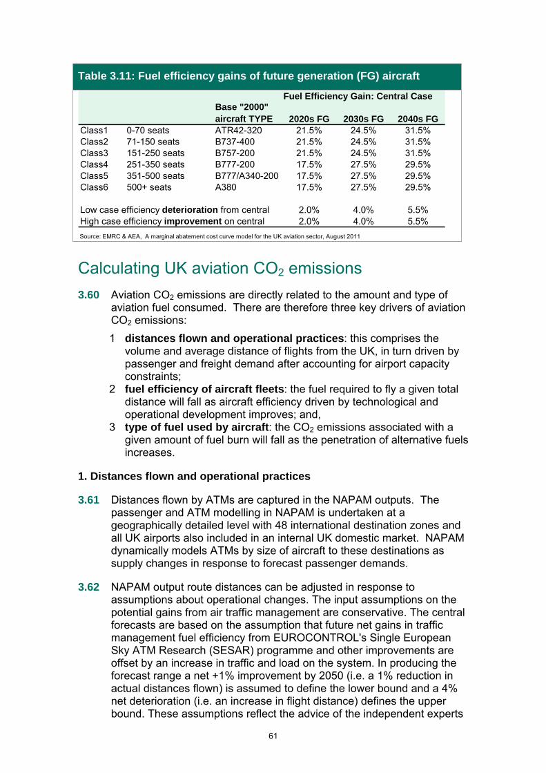
Table 3.11: Fuel efficiency gains of future generation (FG) aircraft
Fuel Efficiency Gain: Central CaseBase "2000" aircraft TYPE 2020s FG 2030s FG 2040s FG
Class1 0-70 seats ATR42-320 21.5% 24.5% 31.5%Class2 71-150 seats B737-400 21.5% 24.5% 31.5%Class3 151-250 seats B757-200 21.5% 24.5% 31.5%Class4 251-350 seats B777-200 17.5% 27.5% 29.5%Class5 351-500 seats B777/A340-200 17.5% 27.5% 29.5%Class6 500+ seats A380 17.5% 27.5% 29.5%
Low case efficiency deterioration from central 2.0% 4.0% 5.5%High case efficiency improvement on central 2.0% 4.0% 5.5%
Source: EMRC & AEA, A marginal abatement cost curve model for the UK aviation sector, August 2011
Calculating UK aviation CO2 emissions
3.60 Aviation CO2 emissions are directly related to the amount and type of aviation fuel consumed. There are therefore three key drivers of aviation CO2 emissions:
1 distances flown and operational practices: this comprises the volume and average distance of flights from the UK, in turn driven by passenger and freight demand after accounting for airport capacity constraints;
2 fuel efficiency of aircraft fleets: the fuel required to fly a given total distance will fall as aircraft efficiency driven by technological and operational development improves; and,
3 type of fuel used by aircraft: the CO2 emissions associated with a given amount of fuel burn will fall as the penetration of alternative fuels increases.
1. Distances flown and operational practices
3.61 Distances flown by ATMs are captured in the NAPAM outputs. The passenger and ATM modelling in NAPAM is undertaken at a geographically detailed level with 48 international destination zones and all UK airports also included in an internal UK domestic market. NAPAM dynamically models ATMs by size of aircraft to these destinations as supply changes in response to forecast passenger demands.
3.62 NAPAM output route distances can be adjusted in response to assumptions about operational changes. The input assumptions on the potential gains from air traffic management are conservative. The central forecasts are based on the assumption that future net gains in traffic management fuel efficiency from EUROCONTROL's Single European Sky ATM Research (SESAR) programme and other improvements are offset by an increase in traffic and load on the system. In producing the forecast range a net +1% improvement by 2050 (i.e. a 1% reduction in actual distances flown) is assumed to define the lower bound and a 4% net deterioration (i.e. an increase in flight distance) defines the upper bound. These assumptions reflect the advice of the independent experts
61

working on the DfT marginal abatement cost curve (MACC) study analysis in 2010-2011.50
3.63 In producing the forecast range some allowance has been made for changes in airline operational practices (e.g. optimised payloads, flying speeds and altitudes) to deliver fuel efficiency gains. No additional improvement has been assumed in producing the central forecast, but +/- 0.25% efficiency improvement in fuel efficiency of future aircraft fleets relative to the central case has been assumed in producing the lower/upper bound of the CO2 emissions forecast.
2. Fuel efficiency of aircraft fleets
3.64 Current fuel burn rates by aircraft type measured in kilograms of fuel per aircraft for different distance bands flown, and for different stages of the flight are initially taken from the European Environment Agency's 'CORINAIR' Emission Inventory Guidebook.51 Seat-kms per mass of fuel (i.e. seat-kms per tonne or kg of fuel) is the preferred metric for measuring aviation fuel efficiency. The value of this metric is that it is essentially unaffected by the assumed or modelled load factors.
3.65 In 2010 a QinetiQ study commissioned by DfT reported on the suitability of the current CORINAIR guidebook rates of fuel burnt by distance band for each CORINAIR aircraft type. The study provided advice on the mapping of specific aircraft types to generic CORINAIR types, adjustments to the fuel burn rates for existing aircraft especially those not well represented in the generic types such as extended range versions of the B777 and the A380. It also provided rates for aircraft expected to enter service in the next decade such as Boeing 787s, Airbus A350s and the Bombardier C Series52 and then the subsequent generations of new aircraft from 2020s onwards. All these recommendations have been retained in the Fleet Mix and CO2 models in these forecasts.
3. Type of fuel used by aircraft
3.66 The updated central forecasts assume that biofuels are gradually introduced in the 2020s and make up 2.5% of all aviation fuel burnt by aircraft departing UK airports in 2050. In defining the lower bound of the forecast range, no biofuels penetration is assumed to 2050, while in defining the upper bound of the range, biofuel penetration is assumed to
50EMRC & AEA, A marginal abatement cost curve model for the UK aviation sector, August 2011 http://assets.dft.gov.uk/publications/response-ccc-report/mac-report.pdf 51 EMEP/CORINAIR Emission Inventory Guidebook - 2006, European Environment Agency http://reports.eea.europa.eu/EMEPCORINAIR4/en/page002.html This is an established and authoritative source of data on aircraft fuel burn rates, giving separate values for the different stages of the flight such as landing and take off including taxiing and cruise emissions for different aircraft types. It is used for general reference and for use by parties to the Convention on Long Range Transboundary Air Pollution (LRTAP) for reporting to the UNECE Secretariat in Geneva. See Future Aircraft Fuel Efficiencies – Review of Forecast Method, QinetiQ on behalf of the DfT, March 2010, Chapter 6. https://www.gov.uk/government/uploads/system/uploads/attachment_data/file/4515/future-aircraft-fuel-efficiency.pdf
62

3.67 Once the above method has forecast the amount of fuel that is burned on flights departing each airport on each route by aircraft type, this is converted into CO2 emissions on the basis that 1.00 kg of kerosene emits 3.15 kg of CO2.
53 Where biofuel uptake is assumed, this average carbon intensity factor is reduced on the assumption that biofuels are accounted for in the transport sector as having zero emissions.54 For example, in the central forecast in 2050 with 2.5% biofuel take up, it is assumed that across the entire fleet 1.00kg of fuel emits 3.07kg of CO2.
CO2 emissions range
3.68 After forecasting the range of ATMs, further assumptions relating to the composition of the fleet and operational practice are applied to extend the outer boundaries of the CO2 emissions range. It should be noted that although these assumptions potentially have some further effect on airline fuel costs and therefore fares, they are not fed back into the National Air Passenger Demand Model at this stage.55 The assumptions made are summarised in Table 3.12:
53 Each 1 kg of kerosene contains 858 g of carbon. Each 1kg of carbon is equivalent to 44/12 or 3.67 kg of CO2. 54 In practice, different biofuel feedstocks have different levels of life-cycle emissions and biofuels use in aviation is expected to result in lower emissions, but not reduce emissions to zero. The approach taken here is consistent with the accounting of biofuel use in the UK’s carbon budgets and in the EU ETS, and with the latest guidance from the International Panel for Climate Change (IPCC). 55 Fleet fuel efficiency is an input to the fares faced by passengers in the National Air Passenger Demand Model because fuel efficiency is an input to the forecasts of fares faced by passengers. Representative fuel efficiencies for the low, central and high demand scenarios from recent (but not final) model runs are used in these fare forecasts. The principle is to use the best available model outputs on fleet fuel efficiency rates while avoiding unnecessary iterations between the demand and CO2 model components of the forecasting framework where changes in output passenger demand would be very small.
63

Table 3.12: CO2 emission variable range assumptions
Low: low demand growth (low oil prices)+
no regulatory CO2 standard;
standard DfT retirement ages of 22 years,56
no retro-fitting;
2020 future generation having a 19.5-23.5% fuel burn improvement on 2000 standard types, the 2030 future generation having a 28.5-31.5% improvement and the 2040 future generation having a 35.0-37.0% improvement;
after ATM growth, SESAR and other programmes achieve a 1% net air traffic management system gain by 2050;
0.25% extra efficiency each year through airline operational efficiency practices; and,
no biofuel use.
Central: central demand growth +
no regulatory CO2 standard;
standard DfT retirement ages of 22 years;
no retro-fitting;
2020 future generation having a 17.5-21.5% fuel burn improvement on 2000 standard types, the 2030 future generation having a 24.5-27.5% improvement and the 2040 future generation having a 29.5-31.5% improvement;
no net air traffic management system gains as improvements from SESAR and other programmes are assumed to accommodate the growth in ATMs without further deterioration in levels of service;
no improvement from airline operational efficiency practices; and,
0.5% biofuel use in 2030 rising to 2.5% by 2050.
56 Based on analysis of DfT analysis of UK fleet turnover using airframe data from CAA. There are some exceptions to 22 years for the earlier retirement of very old types and slightly later retirement for the charter fleet.
64

High: high demand growth (high oil prices)+
no regulatory CO2 standard;
standard DfT retirement ages of 22 years;
no retro-fitting;
2020 future generation having a 15.5-19.5% fuel burn improvement on 2000 standard types, the 2030 future generation having a 20.5-23.5% improvement and the 2040 future generation having a 24.0-26.0% improvement;
a 4% deterioration in the net air traffic management system despite the implementation of SESAR and associated programmes;
0.25% less efficiency each year through airline operational practices; and,
1% biofuel use in 2030 rising to 5% by 2050.
65

4. Unconstrained passenger forecasts
Introduction (what is an unconstrained forecast?)
4.1 The unconstrained forecasts represent underlying estimates of demand in the absence of airport capacity constraints. The forecasts reported here are derived from the National Air Passenger Allocation Model.
Unconstrained passenger forecasts
4.2 The results for million terminal passengers57 per annum (mppa) at the national level are summarised in Table 4.1.58
Table 4.1: UK terminal passenger forecasts (unconstrained), mppa
Low Central High
2010 211 211 2112015 220 230 2402020 240 260 2802025 260 290 3152030 280 320 3602035 295 355 4152040 315 390 4852045 335 435 5652050 350 480 660
Figures in forecast years rounded to nearest 5 mppa.
4.3 Table 4.1 shows that in the absence of capacity constraints the underlying trend of growth in UK air passenger demand is forecast to continue, rising from 211 million passengers per annum (mppa) in 2010 to 320mppa in 2030, within the range 280mppa to 360mppa, and to 480mppa by 2050, within the range 350mppa to 660mppa. Figure 4.1
57 See paragraphs 2.3-2.8 for definition and discussion of the unit of 'terminal passenger'. 58 These are modelled unconstrained passengers after allocation by the National Air Passenger Allocation Model. These will differ from the unconstrained terminal passenger forecasts produced by the input National Air Passenger Demand Model because the National Air Passenger Allocation Model allocates passengers to indirect routes such as via UK hubs where a single one way journey may be counted as three terminal passengers. See paragraphs 2.3-2.8.
66

illustrates the range of unconstrained forecasts graphically. Annex D provides more detailed results.
Figure 4.1: UK unconstrained demand – historic with central, low and high forecasts
0
100
200
300
400
500
600
700
800
1990 1995 2000 2005 2010 2015 2020 2025 2030 2035 2040 2045 2050
UK
te
rmin
al
pa
ss
en
ge
rs,
mp
pa
Forecast range Central forecast
2010 - 2050 1%-3% average
growth
1990 - 2010 4% average
growth
67

5. Constrained passenger and aircraft forecasts
Introduction (what is a constrained forecast?)
5.1 Constrained UK air passenger and ATM forecasts, take into account the effect of the limitations to runway and terminal capacity at UK airports. They are formed by inputting the unconstrained demand forecasts output by the National Air Passenger Demand Model into the DfT National Air Passenger Allocation Model. The assumed capacity constraints at UK airports are outlined in chapter 3 at paragraphs 3.50-3.52.
5.2 Forecasts are presented for the low-central-high range of demand with passengers allocated using the maximum use capacity scenario (see the section on airport capacities in chapter 3). In the high demand case it is not possible for the passenger to airport allocation model to complete forecasting in the later years of the forecast period. When this occurs no results are interpolated and the relevant areas in the table are shaded out. In practice this indicates that all the larger airports across the UK are at capacity.
Passenger forecasts
5.3 The results for million terminal passengers59 per annum (mppa) at the national level are summarised in Table 5.1. This table shows that, after accounting for airport capacity constraints under the ‘max use’ capacity scenario, the number of UK air passengers is forecast to rise to 315mppa in 2030, within the range 275mppa to 345mppa. By 2050, the number of UK air passengers is forecast to reach 445mppa within the range 340mppa to 445mppa.60 Annex E gives more detailed passenger forecasts, and Box 5.1 sets out how these forecasts can be interpreted in terms of future trip-making by air passengers.
59 See paragraphs 2.3-2.8 for definition and discussion of the unit of 'terminal passenger'. 60 Note that the allocation model cannot fit high growth demand to available capacity much beyond 2040, so high growth terminal passengers have been assumed to remain constant after 2043. This is why central and high growth forecasts appear to converge by 2050.
68

Table 5.1: UK terminal passengers forecast, 'max use' capacity, mppa
Low Central High
2010 211 211 2112015 220 225 2352020 235 255 2752025 255 285 3102030 275 315 3452035 290 340 3952040 305 370 4502045 325 4102050 340 445
Figures in forecast years rounded to nearest 5 mppa.
National Air Passenger Allocation Model failed to reach 2050.
Box 5.1: Forecast terminal passengers and journeys
The average number of international air trips taken by each resident in the UK has increased by 5% a year between 1988 and 2008, from just under 0.4 international trips in 1988 to just under 1 trip a year in 2008.61 Converting the unrounded central 2030 forecast of 313 million terminal passengers into trips abroad by UK residents and visits from foreign residents requires a careful application of the definition of terminal passengers set out in paragraphs 2.3-2.8 and also identification of those hub interchanges by passengers who do not stop in the UK (international-international interliners). Applying this definition shows:
UK residents make 1.24 overseas trips by air per person using the ONS estimate of 70m UK residents in 2030. This equates to 176m terminal passengers.
There would be 34m foreign visits by air compared with the current 23m foreign visits accounting for 69m terminal passengers.
Domestic journeys are counted at two UK airports, so 41m terminal passengers account for 10m internal domestic return air journeys or 1 domestic flight for every 7 UK residents in 2030.
Finally, there would be 6.75m return journeys (equating to 27m terminal passengers) by international-international interliners using UK hub airports to make connections without stopping in the UK - up from the current level of 5.5m return connections (or 22m terminal passengers).
61 Estimates of the exact number of international air trips per person vary between sources. These are "backcast" numbers for consistency with the forecast to 1988 using the growth rates from the International Passenger Survey completed by the Office of National Statistics. See also Table TSGB0113 in
69

5.4 Figure 5.1 further illustrates the range of updated UK air passenger forecasts for the ‘max use’ capacity scenario. A comparison of the constrained forecasts presented in Table 5.1 and Figure 5.1 with the unconstrained forecasts in Table 4.1 and Figure 4.1 shows that the assumed future airport capacities constrain forecast throughput at UK airports, and that the impact of this increases through time. In the central forecasts, airport capacity constrains national throughput by 5mppa in 2030 rising to 35mppa by 2050. At the lower end of the forecast range, capacity is forecast to constrain airport throughput by 5mppa in 2030 and by 10mppa in 2050. At the upper end of the forecast range, airport capacity constrains throughput by 15mppa in 2030 and 220mppa in 2050.
Figure 5.1: UK terminal passengers (constrained – ‘max use’) - historic with central, low, and high forecasts
0
50
100
150
200
250
300
350
400
450
500
1990 1995 2000 2005 2010 2015 2020 2025 2030 2035 2040 2045 2050
UK
te
rmin
al
pa
ss
en
ge
rs,
mp
pa
Forecast range Central forecast
2010 - 2050 1%-2% average
growth
1990 - 2010 4% average
growth
5.5 No high growth results are presented after 2040 as the model suggests that the airport system has become overloaded by around that time. In the maximum use of existing capacity scenario this tends to happen with national throughputs of about 450 million terminal passengers. As Figure 5.1 illustrates, this level of saturation is reached around 2050 with central demand but is not reached in the forecast period at the lower end of the demand range.
https://www.gov.uk/government/publications/transport-statistics-great-britain-2012 for more information on current levels of trip by UK residents and foreign visits by air and other modes.
70

International and domestic passengers
5.6 Table 5.2 splits international passengers by length of haul. It analyses the ultimate passenger destination and classifies (for example) passengers who use a European hub airport such as Amsterdam Schiphol, Paris Charles de Gaulle or Frankfurt en route to a long haul destination as being long haul. Table 5.2 shows that the proportion of long haul journeys varies between 27%-29%. The long haul proportion increases over time as short haul demand tends to use smaller aircraft and these aircraft are more likely to be displaced as airports become runway constrained.62 Such passengers are modelled as either not travelling or using more distant and less preferred airports. The largest reduction occurs to the hub transfers as these passengers incur the penalty of utilising constrained runways twice as they interchange at the hub.
Table 5.2: International terminal passengers, 2010 to 2050 (mppa) by length of haul
Low Central High Low Central High Low Central High Low Central High2010 119 119 119 36 36 36 29 29 29 183 183 1832020 135 148 160 42 46 50 31 29 28 208 223 2382030 159 183 201 50 58 64 35 31 27 244 272 2922040 178 220 261 56 71 88 37 30 26 271 322 3752050 197 263 64 89 39 37 300 388
National Air Passenger Allocation Model failed to reach 2050.
Short Haul Long Haul TotalYear
Transfers
5.7 A similar effect is apparent in the breakdown between the international and domestic passenger markets shown in Table 5.363 and Figure 5.2 if the hub transfers are excluded from the international totals. Like short haul international passengers, domestic passengers are carried on smaller aircraft and the majority have one journey end in an area of the UK with congested airports, so are therefore also more likely to be displaced by runway constraints.
Table 5.3: International and domestic constrained passengers, 2010-2050 (mppa)
Low Central High Low Central High Low Central High2010 183 183 183 27 27 27 211 211 2112020 208 223 238 28 32 38 236 255 2772030 244 272 292 32 41 55 276 313 3472040 271 322 375 35 50 76 306 372 4512050 300 388 39 59 339 447
National Air Passenger Allocation Model failed to reach 2050.
International Domestic TotalYear
62 The fare premium applied to airports with overloaded runways is charged on a per plane basis. With larger aircraft (e.g. those on long haul routes) the fare premium is split among more passengers and therefore is lower on a per passenger basis making routes using larger aircraft more resilient to increasing fare premia. 63 The analysis defines domestic passengers as those making journeys within the UK and does not include those using domestic services to transfer to an international flight at a UK hub.
71

Figure 5.2: Domestic and international constrained passengers, 2000-2050 (mppa)
0
50
100
150
200
250
300
350
400
450
500
2000 2005 2010 2015 2020 2025 2030 2035 2040 2045 2050
mp
pa
International low
International central
International high
Domestic low
Domestic central
Domestic high
Historical data
5.8 It is usually more informative to examine the changing patterns of international and domestic demand on the basis of constrained forecasts. Some equivalent analysis of unconstrained passenger demand has been made and this is presented in Annex D.
Business and leisure passengers
5.9 Table 5.4 below and Figure 5.3 show both UK and foreign resident passengers split between business and leisure journey purposes for international journeys across the forecast range. At present 80% of air passenger journeys beginning or ending in the UK are for leisure purposes. This split is forecast to change only very slightly by 2050 with leisure purposes continuing to represent 79% of international air trips to and from the UK across the forecast range of demand. However leisure passengers are more likely to switch airport and make longer airport access journeys as congestion rises and therefore the results of this analysis at individual airports vary more significantly than at the national level.
72

Table 5.4: Constrained international forecasts of passengers, 2010-2050 by purpose (mppa)
Low Central High Low Central High2010 147 147 147 36 36 362020 166 176 187 42 47 512030 195 214 225 49 58 672040 217 254 290 54 68 852050 240 307 60 81
National Air Passenger Allocation Model failed to reach 2050.
Year
Leisure (mppa) Business (mppa)
Figure 5.3: Constrained international forecasts of passengers by purpose, 2000-2050 (mppa)
0
50
100
150
200
250
300
350
400
2000 2005 2010 2015 2020 2025 2030 2035 2040 2045 2050
mp
pa
Leisure low
Leisure central
Leisure high
Business low
Business central
Business high
Historic data
5.10 Figure 5.4 provides a similar analysis for the forecast range of air passengers internal to the UK. Internal domestic flights are much more evenly split between business and leisure purposes. This split is not forecast to change greatly, but the share of business passengers is expected to grow modestly over time. This analysis is confined to passengers travelling internally within the UK. It excludes passengers using domestic flights to transfer to international connections who are counted in the international forecasts. If these passengers had been
73

included in this analysis then Figure 5.4 would show leisure passengers slightly outnumbering business passengers in most demand cases.64
Figure 5.4: Constrained domestic forecasts of passengers, 2000-2050 (mppa) by purpose
0
5
10
15
20
25
30
35
40
45
2000 2005 2010 2015 2020 2025 2030 2035 2040 2045 2050
mp
pa
Leisure low
Leisure central
Leisure high
Business low
Business central
Business high
Historic Business data
Historic Leisure data
5.11 It is usually more informative to examine the changing patterns of demand by different journey purposes on the basis of constrained forecasts. However, some equivalent analysis of unconstrained passenger demand has been made and this is presented in Annex D.
64 It is not appropriate to count the domestic-international transfers in the domestic category because if airports become constrained or more attractive direct routes start up or more attractive surface connections to alternative airports become available then these passengers disappear from domestic flights.
74

5.12 Figure 5.5 below shows the proportions of the regional destinations of business and leisure respectively. Internal domestic flights are more significant for business passengers while Western Europe attracts a noticeably lower proportion of business passengers than for leisure purposes.
Figure 5.5: Business and leisure shares by region, 2010 & 2030 (mppa)
Business Travel
52.5% 53.3% 52.9% 51.1%
10.3% 10.5% 9.6%9.0%
2.7% 3.0% 2.8%2.7%
7.6%9.1% 9.0%
8.7%
26.9% 24.1% 25.6% 28.5%
0%
10%
20%
30%
40%
50%
60%
70%
80%
90%
100%
2010 2030 Low 2030 Central 2030 High
Western Europe OECD (Non-European) Newly Industrialised Countries
Less Developed Countries Domestic (UK only)
Leisure Travel
66.0% 66.4% 66.2% 65.0%
11.3% 11.7% 10.9% 10.4%
3.0% 3.3% 3.2%3.1%
11.2% 10.9% 10.7%10.4%
8.6% 7.7% 9.0% 11.1%
0%
10%
20%
30%
40%
50%
60%
70%
80%
90%
100%
2010 2030 Low 2030 Central 2030 High
Western Europe OECD (Non-European) Newly Industrialised Countries
Less Developed Countries Domestic (UK only)
75

Passengers at UK airports
5.13 The National Air Passenger Allocation Model forecasts how passenger demand will be distributed in a system-wide manner between airports around the UK, after accounting for likely airport capacity constraints. Table 5.5 below shows the central airport forecasts to 2050 for the South East and other larger UK airports, under the central 'max use' capacity scenario. It shows that between 2030 and 2040 airport passenger growth at the London airports is forecast to almost cease as they reach full capacity.65 After 2040 growth is only forecast to occur at airports outside the South East. Annex E shows the results for each modelled UK airport.
5.14 The model is tasked with finding an equilibrium balance between demand and available capacity for all airports in the system. At times, particularly later in the period, this means that some limited variations around input passenger capacity are permitted to allow the modelling to converge at an equilibrium solution, resulting in some forecasts shown here or in Annex E being marginally over input capacity.
5.15 Unrounded forecasts are presented in Annex E. This is primarily to give transparency to modelling outputs. The use of unrounded figures does not reflect the underlying level of certainty around individual results.
65 While the airports are effectively full, there is still some growth as a result of some further increases in aircraft sizes and load factors.
76

Table 5.5: UK terminal passenger forecasts (mppa) at principal UK airports, 2011-2050, ‘max use’, (central forecast)
Airport 2011 2020 2030 2040 2050
Heathrow 66 75 82 87 93Gatwick 31 37 41 43 44Stansted 19 25 36 36 35Luton 9 14 18 19 18London City 3 5 6 6 7Southend 0 2 3 2 2London 128 158 186 193 199annual growth rate 2.4% 1.6% 0.4% 0.3%
Manchester 18 22 28 39 55Birmingham 9 12 17 28 38Glasgow 7 7 9 10 12Edinburgh 9 11 13 17 20Bristol 6 7 10 12 12Newcastle 4 4 5 6 9Belfast International 4 5 7 8 10Liverpool 5 5 7 8 15East Midlands 4 4 4 9 14Other modelled 15 20 27 42 63
2.0% 2.7% 3.5% 3.3%
Total 209 255 313 372 4472.2% 2.0% 1.7% 1.9%
Non-London annual growth rate
annual growth rate
5.16 As demand grows the airports fill until they become constrained by limits either on the terminal or runway capacities. Table 5.6 shows a similar analysis of the larger airports for the low and high ends of the forecast range. High growth is shaded out after 2040 because no model results are possible after the early 2040s as demand rises over 450mppa. At this point over 90% of national passenger capacity in the 'maximum use' scenario is being used.
5.17 The central forecasts suggest that all the South East airports would be at capacity at around 2030 and the larger airports outside the South East from about 2040. At the low end of the forecast range, the South East airports in total are at capacity by 2040. The high range forecast is that the South East airports are full by 2025.
77

Table 5.6: Low-high range of UK terminal passenger (mppa) forecasts at principal UK airports, 2020-2050, ‘max use’ capacity scenario
2020 2030 2040 2050 2020 2030 2040 2050
Heathrow 75 80 85 89 74 82 91Gatwick 39 39 40 41 40 41 44Stansted 21 30 36 35 29 35 34Luton 11 15 19 18 15 18 18London City 3 7 7 7 6 7 7Southend 1 2 2 2 2 2 2London 150 173 189 192 166 185 196annual growth rate 1.6% 1.4% 0.9% 0.2% 2.6% 1.1% 0.6%
Manchester 20 24 28 33 24 32 57Birmingham 10 11 14 19 14 25 36Glasgow 6 7 8 9 8 10 14Edinburgh 10 11 13 15 12 16 21Bristol 6 8 9 11 8 12 12Newcastle 4 4 5 5 5 6 8Belfast International 4 5 6 7 6 8 11Liverpool 5 5 6 7 6 8 15East Midlands 3 4 4 6 4 6 14Other modelled 18 24 24 35 24 39 67Non-London annual growth rate 0.6% 1.8% 1.3% 2.2% 3.2% 3.9% 4.7%
Total 236 276 306 339 277 347 451annual growth rate 1.2% 1.6% 1.1% 1.0% 2.8% 2.3% 2.7%
National Air Passenger Allocation Model failed to reach 2050.
High end of rangeLow end of rangeAirport
5.18 The first airports to fill are in the London area. Table 5.7 uses the constrained central forecasts shown above in Table 5.5 and relates this demand to the maximum use scenario runway capacities given in Table 3.10. It illustrates when the London airports become full and how the airports most affected by 'spill' from the South East react. Similar analysis for the low and high ends of the demand range is included in Annex E.
78

Table 5.7: UK airports runway capacity used, 2011-2050, ‘max use’ capacity scenario (central forecast)
Airport 2011 2020 2030 2040 2050
Heathrow 99% 100% 100% 100% 100%Gatwick 90% 100% 100% 100% 100%Stansted 58% 69% 100% 100% 100%Luton 59% 60% 100% 100% 100%London City 56% 87% 100% 100% 100%Southend 42% 100% 100% 100%London 81% 86% 100% 100% 100%Manchester 49% 57% 55% 58% 100%Birmingham 45% 56% 79% 100% 100%Bristol 35% 38% 37% 100% 100%East Midlands 22% 17% 20% 43% 100%Southampton 27% 36% 52% 100% 100%Other modelled 22% 24% 28% 33% 43%National 39% 43% 50% 54% 63%100% = runway or terminal capacity exceeded, other %s refer to runway usage.
Mainland UK airports only.
5.19 As airports fill up and become constrained passengers either re-allocate to a less preferred airport or are deterred by the increased prices at the constrained airports from travelling altogether. Figure 5.6 shows the geographic distribution by district of proportions of passengers who were suppressed from travelling by capacity constraints for the central case forecasts in 2040.
79

Figure 5.6: Proportions of air passengers suppressed from travel by district, 2040, (central demand)
International destinations served from the UK
5.20 As described in chapters 2 and 9, the airport allocation model has been calibrated to replicate as close as possible the number of international destinations served by each airport in the model validation year of 2011. This allows the model to make a useful estimate of how this range of destinations might increase in response to future changes in demand.
80

5.21 Table 5.8 reports how the number of destinations served with at least daily services at a selection of the larger airports changes. It rises with demand at airports which are less capacity constrained, but contracts at the most constrained airports where routes consolidate and destinations served by smaller aircraft get squeezed out by runway slot constraints. It should be noted that this analysis does not include domestic routes but does count both charter and scheduled destinations. A more disaggregate breakdown by type of carrier (full service scheduled, low cost and charter) is available in Annex E.66
Table 5.8 : Modelled international destinations served at selected UK airports, 2011, 2030 & 2050, central demand
2011* 2030 2050Heathrow 135 136 121Gatwick 79 86 83Stansted 56 74 68Luton 26 42 31London City 17 22 14Southend 0 5 4London** 178 212 230
Manchester 40 65 105Birmingham 21 40 67Glasgow 6 6 12Edinburgh 11 20 31Newcastle 6 8 17Belfast International 2 9 16Bristol 13 28 41Liverpool 15 23 35East Midlands 7 9 54Other modelled airports 22 49 78
Total** 178 215 242
**Total different destinations available, not sum of individual airport destinations
All types of carrier
* 2011 is modelled. Modelled numbers will vary slightly from observed patterns because they represent a full year of operation: observed data will include seasonal services and new start-ups or routes withdrawn during the course of the year.
66 Unlike Table 5.8, the counting of routes in Annex E is made on the basis of routes with more than 5,000 passengers to the destinations and each destination counted separately for the full service scheduled, low cost and charter airline markets. The style of presentation of using a passenger number threshold in Annex E is compatible with the validation exercise reported in Table 9.6 and Annex B.
81

ATM forecasts
5.22 Forecast ATMs are highly dependent on the forecasts of passengers, routeings and passenger loads on aircraft. Table 5.9 and Figure 5.7 show the forecast range for ATMs to 2050. The ATM forecasts are presented at a more detailed airport level in Annex F.
5.23 Table 5.9 shows that in common with the constrained passenger forecasts, the high ATM forecast is flat relative to the central forecast in the later years. This is because in the high forecast the major airports are unable to accommodate further runway movements in the 2030s and 2040s. It is assumed that relatively little of this activity can transfer to the smaller airports once the medium sized regional airports are full.
Table 5.9: Range of UK ATM (000s) forecasts, 2010-2050
000s ATMs Low Central High
2010 2,000 2,000 2,0002015 2,000 2,100 2,2002020 2,100 2,300 2,5002025 2,300 2,500 2,7002030 2,400 2,700 3,0002035 2,500 3,000 3,4002040 2,700 3,200 3,8002045 2,900 3,500 3,8002050 3,000 3,800 3,800
Figures in forecast years rounded to nearest 100 thousand ATMs.
National Air Passenger Allocation Model failed to reach 2050.
5.24 When the high range model runs cease in the 2040s, 85% of runway and 88% of terminal capacity are used. Only eight airports are not fully utilised and these are generally the most distant from the South East.67 Extrapolating ATMs to fill the last runway remaining capacity would give a misleading result because of the specialised and niche markets served by these airports.
67 In the model these are the two Northern Ireland airports, three Scottish airports, the two North East airports and Newquay. Many of these have significant and distinctive domestic markets or are 'niche' destinations.
82

Figure 5.7: Projected range of constrained ATM demand to 2050
0
1000
2000
3000
4000
1990 1995 2000 2005 2010 2015 2020 2025 2030 2035 2040 2045 2050
UK
AT
Ms
(0
00
s)
Forecast range Central forecast
2010 - 2050 1%-2% average
growth1990 - 2010 2% average
growth
83
6. CO2 emissions forecasts
Nature and purpose of forecasts
6.1 There is currently no internationally agreed way of allocating international emissions to individual countries. The DfT forecast carbon dioxide (CO2) emissions produced by all flights departing UK airports to 2050, adjusted to match the DECC estimate of outturn (i.e. published) aviation CO2 emissions (using the UNFCCC reporting method) in the base year,68 as reported in the National Atmospheric Emissions Inventory (NAEI).69 The forecasts therefore include CO2 emitted from all domestic flights within the UK, and all international flights which depart UK airports, irrespective of the nationality of passengers or carriers.
6.2 The forecast of aviation CO2 covers emissions from aircraft. It does not include related emissions from journeys to and from UK airports which are recorded in different parts of the UK national inventory.70
68 This covers the 31 largest airports in the UK. Emissions from the other minor airports are unlikely to be significant as they offer only short range services. DECC's estimates of outturn CO2 emissions from aviation are based on the amount of aviation fuel uplifted from bunkers at all UK airports. The 'forecast' for 2008 is about 0.5MtCO2 (1%) below the latest revised DECC estimate for that year. This residual amount is added back into the forecasts. A similar procedure is required by DECC when converting air fuel sales data to CO2 bunker emissions data for domestic and international civil aviation. In the modelling the normalisation also reflects any difference in definition, including the absence from the modelling of the minor types of traffic such as business jets which are difficult to model, or flights from very small airports that are not included in the model. 69 See www.naei.org.uk/. In the NAEI, UK domestic aviation CO2 emissions are reported in the UK total and international aviation emissions are reported as a memo item. 70 The CO2 forecasts in this report relate specifically to aircraft both on the ground and in the air. However, in appraising potential policy measures affecting capacity/level of activity at specific airports the DfT also considers the potential for significant impacts on CO2 emissions from airport surface access.
84

6.3 The sources of emissions covered in the forecasts in this chapter are set out in Table 6.1 below.
Table 6.1: Definition of CO2 emissions in the forecasts
Emissions source Included in the forecasts?
All domestic passenger flights departing within the UK71
All international passenger flights departing UK airports
All passenger aircraft while on the ground in the UK e.g. taxiing
All domestic freighter aircraft departing UK airports
All international freighter aircraft departing UK airports72
All freighter aircraft while on the ground in the UK e.g. taxiing
General aviation (non commercial flights) in UK airspace
Surface access, i.e. passenger and freight journeys to and from a UK airport
Non-aircraft airport sources, e.g. terminal lighting and airfield vehicles
UK registered aircraft flying from airports not in the UK
International flights arriving in the UK
Over-flights passing through UK airspace
6.4 CO2 emission forecasts are presented based on the low-high range of passenger demand allocated to the maximum use of existing airport capacity scenario (see the section on airport capacities in chapter 3). In the high demand case it is not possible for the passenger to airport allocation model to complete forecasts in the later years of the period. When this occurs no results are interpolated and the relevant areas are greyed out. In practice this indicates that all the larger airports across the UK are at capacity.
6.5 The scope of the CO2 emissions modelling is aircraft departing UK airports. Although forecasts are produced of numbers of UK transfer passengers opting to use foreign hubs, there are no forecasts of aircraft departing foreign hub airports from which robust assessments associated with the full onward journey of UK passengers emissions could be calculated.73
71 Emissions from return domestic flights are counted as two UK departures rather than from total arrival and departure ATMs reported at UK airports. An estimate on this basis would double-count domestic aviation emissions. 72 Emissions from freight carried in the belly hold of aircraft are captured in the passenger aircraft emissions. 73 Suitable emissions forecasts from continental hub airports affected by changing patterns of UK passenger movement would require modelling of ATMs at overseas airports. This requires estimates of
85

Context of aviation greenhouse gas emissions
6.6 The DfT’s UK aviation CO2 emission forecasts are used to help monitor and inform long-term strategic UK aviation and climate change policy. Recent forecasts have been central to the Government's response to the Committee on Climate Change (CCC) report.74 These forecasts will support the ongoing work on the development of the Government's sustainable framework for UK aviation (Aviation Policy Framework).
6.7 This section sets out how aviation’s greenhouse gas emissions have grown and how they currently compare to total greenhouse gas emissions at the national and global level.
6.8 CO2 makes up about 99 per cent of the Kyoto greenhouse gas emissions from UK aviation.75
6.9 Figure 6.1 shows UK aviation emissions in million tonnes of carbon dioxide (MtCO2) since 1970 to 2010, the latest year for which NAEI bunker fuel returns are available. It demonstrates that in keeping with the global growth in demand for air travel discussed in Chapters 2 and 3, CO2 emissions have tended to grow strongly. Some deviations from the trend are evident, and these are explained by demand variations, such as those resulting from the oil price shocks in the 1970s, recessions, terrorism threats or fears of global pandemics. The unprecedented reduction in aviation CO2 emissions following the recent financial crisis and economic recession is clearly visible. Figure 6.1 also shows that international travel from the UK, as opposed to domestic flights, has been the main source of emissions growth, consistently accounting for over 90% of aviation emissions.
future service patterns, future fleet mixes and future pressure on capacity at overseas hub airports. This is beyond the scope of DfT modelling. 74 Government Response to the Committee on climate change’s report on reducing emissions from UK Aviation to 2050, Department for Transport, August 2011 75 UK Greenhouse Gas Emissions, Department of Energy & Climate Change, 2011 2010 Inventory Tables - UK Greenhouse Gas Statistics. http://www.decc.gov.uk/en/content/cms/statistics/climate_stats/gg_emissions/uk_emissions/uk_emissions.aspx
86

Figure 6.1: Aviation CO2 emissions, MtCO2, 1970-2010
0
5
10
15
20
25
30
35
40
1970 1975 1980 1985 1990 1995 2000 2005 2010
Mil
lio
n t
on
nes
of
carb
on
dio
xid
e
International
Domestic
6.10 While aviation is currently a relatively small contributor to total greenhouse gas emissions (both at the UK and global levels), the projected continuing growth in its emissions alongside projected reductions in other sectors means that aviation’s contribution could increase significantly in the coming decades.
6.11 Available evidence indicates that the aviation sector is responsible for approximately one to two per cent of global greenhouse gas emissions.76 At the UK level, in 2010 domestic aviation accounts for 0.3% of UK greenhouse gas emissions. If internal shipping and international aviation emissions are added to the total in 2010, UK aviation (domestic and international) accounted for 5.4% of UK GHG emissions. This compares to the total for UK transport of 27.1%.77
6.12 As with the passenger forecasts, the CO2 projections are intended to capture the long-term trend in UK aviation CO2 emissions. While they can capture some short-term effects to the extent that the factors driving changes in aviation can be accurately forecast, they are not primarily intended to predict short-term deviations from the trend, as could be caused by further unforeseen recessions or other external shocks.
6.13 There are significant uncertainties about the future path of the factors driving changes in aviation CO2 emissions. As with the air passenger forecasts, this uncertainty is reflected by presenting the CO2 forecasts as a further range around the range already presented for the ATM and
76 Reducing Transport Greenhouse Gas Emissions: Trends and Data, International Transport Forum, 2010 http://www.internationaltransportforum.org/Pub/pdf/10GHGTrends.pdf/ Aviation and Marine Transportation: GHG Mitigation Potential and Challenges, Pew Center on Global Climate Change, 2009 http://www.pewclimate.org/docUploads/aviation-and-marine-report-2009.pdf. 77 UK Greenhouse Gas Emissions, Department of Energy & Climate Change, 2011 - 2010 Inventory Tables - UK Greenhouse Gas Statistics. http://www.decc.gov.uk/en/content/cms/statistics/climate_stats/gg_emissions/uk_emissions/uk_emissions.aspx
87

3.
Other greenhouse gases
6.14 Although aviation does not emit significant quantities of any other Kyoto greenhouse gases, it results in other emissions that have both cooling and warming effects on the climate. These effects come about as a direct result of the atmospheric conditions in which they are emitted. Non-CO2 emissions with climate impacts include water vapour and nitrogen oxides (NOx). Emissions of NOx result in the production of ozone (an air pollutant with harmful health and ecosystem effects and a greenhouse gas), but also the reduction of ambient methane which has a cooling effect. The current understanding is that the overall balance of NOx is warming.
6.15 The last major international assessment of these impacts was made by the Intergovernmental Panel on Climate Change (IPCC) in 1999. A comprehensive updated assessment of aviation emissions was undertaken by Lee et al in 2009.78 CCC (2009) summarises the findings of Lee et al (2009), including its estimates of the different climate effects of aviation.79 For example, the estimated 100-year Global Warming Potentials from Lee et al (2009) indicate that, once the non-CO2 climate effects of aviation are taken into account, aviation’s overall climate effects could be up to double the climate effect of its CO2 emissions. However, while scientific advances since the 1999 assessment have reduced key uncertainties, considerable scientific uncertainty still remains. The latest advice from Lee et al has been not to apply a multiplier to the CO2 emission forecasts.
CO2 forecasts
National
6.16 Table 6.2 reports the central forecast and overall forecast range for CO2 emissions from UK aviation to 2050. The forecast range combines the range of ATM forecasts (explained in chapter 3), with alternative assumptions relating to the composition of the fleet and operational practises explained in paragraph 3.68.
6.17 Table 6.2 shows that under the central forecast aviation emissions rise from 33.3MtCO2 in 2010 to 43.0MtCO2 in 2030, within the range 39.7MtCO2 to 48.2MtCO2. After 2030, the growth in aviation CO2 emissions is forecast to slow as the effects of market maturity and airport capacity constraints cause the growth of activity at UK airports to slow. At
78 Lee et al. (2009) Aviation and global climate in the 21st century, Atmospheric Environment. http://www.tiaca.org/images/tiaca/PDF/IndustryAffairs/2009%20IPCC%20authors%20update.pdf 79 Committee on Climate Change (2009) Meeting the UK aviation target – options for reducing emissions to 2050.
88

the same time fuel efficiency gains continue with aircraft design improvement and the carbon intensity of emissions reducing with the introduction of biofuel. By 2040, the balance of these effects causes emissions to stabilise, before starting to fall by 2050. The forecasts suggest that, in 2050, UK aviation CO2 emissions will reach 47.0MtCO2, within the range 34.7MtCO2 to 52.1MtCO2.
Table 6.2: UK Aviation CO2 forecasts to 2050, MtCO2
Low Central High2010 33.3 33.3 33.32020 36.3 39.4 42.52030 39.7 43.5 48.22040 38.7 46.4 56.92050 34.7 47.0 52.1
*2050 high CO 2 forecast assuming ATMs capped to 2043 level
6.18 Figure 6.2 presents the range of aviation CO2 forecasts alongside historic aviation CO2 emissions.
Figure 6.2: Range of UK aviation CO2 forecasts
0
10
20
30
40
50
60
70
1990 1995 2000 2005 2010 2015 2020 2025 2030 2035 2040 2045 2050
CO
2 e
mis
sio
ns,
MtC
O2
Forecast range Central forecast
6.19 High range ATMs are not forecast beyond 2043, because, as described in paragraphs 5.23-0, the total UK runway capacity is 85% used and using the last remaining capacity would produce a misleading pattern of traffic. In this situation ATMs are frozen at their 2043 level for the period 2044-2050, but the CO2 modelling continues on these ATMs assuming the continuation of the fuel efficiency gains which result from the turnover of the fleet and replacement of older less efficient types by the latest aircraft.
89

Airport level
6.20 As explained above, the national forecast of UK aviation CO2 emissions is based on detailed forecasts of passenger and ATM demand at the airport level. Table 6.3 presents the central CO2 emissions forecasts to 2050, for the largest of the UK's airports.
Table 6.3: CO2 emissions from departing aircraft at individual airports (central forecast)
2010 2030 2050 2010 2030 2050Heathrow 18.8 21.4 18.2 57% 49% 39%Gatwick 3.9 4.7 4.3 12% 11% 9%Stansted 1.1 3.5 1.9 3% 8% 4%Luton 0.7 1.3 0.9 2% 3% 2%London City 0.2 0.5 0.5 1% 1% 1%London Total 24.7 31.4 25.7 75% 72% 55%Other UK Airports 6.9 10.3 19.5 21% 24% 42%Ground APU 0.4 0.5 0.7 1% 1% 2%Freight 0.8 1.2 0.9 2% 3% 2%Residual 0.1 0.1 0.1 0% 0% 0%Total 32.85 43.50 46.97 100% 100% 100%
Emissions million tonnes CO2 Share of Total UK Departure CO2
6.21 Table 6.3 shows that in 2010 London airports accounted for 75% of total UK aviation CO2 emissions. This is forecast to decline to 72% by 2030 and then to 55% by 2050. This is because in the ‘max use’ capacity scenario, growth in aircraft movements is largely only possible at regional airports after 2030. Airports such as Heathrow and Gatwick cannot increase their ATMs because they are at capacity, but they benefit from the fuel efficiency gains as new generations of aircraft enter the fleet. At present Heathrow accounts for around half of the UK's aviation CO2 emissions. This reflects its large share of traffic (around a fifth) and its larger proportion of long haul flights. In the longer term these shares are forecast to decline.
Fuel efficiency
6.22 Table 6.4 shows the penetration of the new aircraft across UK based aviation activity after their introduction in the 2020s and their contribution to aviation emissions. The ‘new aircraft’ are termed ‘FG’ elsewhere in the modelling and refer to aircraft types which enter the fleet for the first time from separate production cycles in the 2020s, 2030s and 2040s. They are distinct from the ‘known’ new types expected to enter service in the next ten years such as the wide-bodied Boeing 787 and Airbus 350 families, and narrow-bodied new generations of Boeing 737s and Airbus A320s and the new Bombardier C Series.80
80 These types are discussed more fully in Future Aircraft Efficiencies – Final Report, QinetiQ, March 2010, but note that the precise efficiency improvements described there have been superseded by the MAC curve analysis reported in Marginal Abatement Cost Curve Model for the UK Aviation Sector, Technical Report, EMRC/AEA, July 2011.
90

Table 6.4: Proportion of aircraft-kms output by future generation ('FG') aircraft, 2020-2050
2020 2030 2040 2050Low 0% 18% 44% 88%Central 0% 20% 44% 82%High 0% 18% 45% 79%
Aircraft-kms
6.23 Table 6.5 shows the range of annual average fuel efficiency improvements underpinning the updated forecasts. It shows that under the central forecasts average fleet fuel efficiency improves by 8% between 2010 and 2030, equivalent to 0.3% a year, with efficiency gains accelerating in the 2020s as the current fleet is largely replaced. The fuel efficiency improvements of future aircraft were based on the DfT's marginal abatement cost curve (MACC) analysis in 2011 which had built on work by QinetiQ in 2010.81
Table 6.5: Annual average fuel efficiency improvements to 2050
Year
IPCC 1999
Low Central High
2010-2020 0.0% -0.1% -0.3% 1.00%
2020-2030 0.8% 0.9% 0.7% 0.50%
2010-2030 0.3% 0.3% 0.1% 0.90%
Aggregate 2010-2030 8.7% 8.1% 3.3%2030-2040 pa 1.4% 1.0% 0.7%2040-2050 pa 2.3% 1.8% 1.5%Aggregate 2010-2050 pa 1.0% 0.8% 0.6%
Annual average
DfT passenger demand range forecasts 2008
6.24 The DfT forecast fuel efficiency is significantly below that predicted by the widely referenced IPCC study in 1999 for the period to 2030. But the IPCC had forecast efficiencies primarily to 2010 based mainly on research published in the early 1990s and based on technical data on
81 Marginal Abatement Cost Curve Model for the UK Aviation Sector, Technical Report, EMRC/AEA, July 2011; Future Aircraft Fuel Efficiencies – Review of Forecast Method, QinetiQ, March 2010.
91

energy use by aircraft operating between 1970 and 1989.82 The previous report, UK Aviation Forecasts, August 2011 explored the reasons for the lower expectations for efficiency improvement than those of the IPCC.83 Essentially it is because the introduction of new aircraft models into the world fleet has been much slower than the IPCC anticipated.84
6.25 More recent work by ICAO/CAEP Modelling and Data Task Force (MODTF) suggests that without significant new aircraft in the fleet before 2016 fuel burn efficiency improvements are likely to be around 0.6% a year rising to 1.0% a year with new ‘known’ aircraft such as Boeing 787s.85 This corresponds closely with the efficiencies running through DfT modelling.
6.26 The structure of the Fleet Mix Model (FMM) can contribute to an understatement of fuel efficiency gains in the first decade of the modelling period shown in Table 6.5. This is essentially a model construct caused by simplifications in the seat categories passed by the airport allocation model to the FMM. This is explained in UK Aviation Forecasts, August 2011.86 It means that the forecast fuel efficiency improvements presented in Table 6.5, are likely to be slightly understated, particularly in the early forecasting period. So while Table 6.5 implies a gradual worsening of fuel efficiency between 2010 and 2020 under the central and high forecasts, this could, more realistically, be interpreted as a very slight improvement in efficiency over the period, especially as recent world economic conditions have incentivised airlines to accelerate the retirement of their more fuel inefficient aircraft.
6.27 It should also be noted that there is not a feedback loop to the demand model for fuel efficiency. The efficiency index shown in Annex C is based on the immediately previous interim CO2 model outputs.
82 Greene, D.L. 1992: Energy-efficiency improvement potential of commercial aircraft in Annual Review of Energy and the Environment, USA, pp.537-574. 83 Aviation and the Global Atmosphere, IPCC, 1999, Table 9-2, p.302. Note also that IPCC (but not Greene) imply that improvements in passenger management and operational efficiencies may have contributed to the fuel efficiency rates (p.302). No such improvements are included in the central forecasts, but alternative assumptions about the scope for improvements in air traffic management and airline operating efficiency are reflected in the overall forecast range . 84 Paragraphs 3-47-3.48 of UK Aviation Forecasts, August 2011, http://assets.dft.gov.uk/publications/uk-aviation-forecasts-2011/uk-aviation-forecasts.pdf. 85 CAEP/8-IP/8 Environmental Goals Assessment Report by MODTF to the Eighth Meeting of CAEP February 2010. See Appendix P. 86 Paragraph 3.49 UK Aviation Forecasts, August 2011.
92

7. Sensitivity tests
Approach
7.1 As with any forecasting exercise looking so far into the future, there is uncertainty over the path the driving variables will follow. Therefore a range of values around the central projection has been considered for the following key variables:
economic growth;
oil prices;
air fares; and,
market maturity assumptions.
7.2 These sensitivity tests illustrate the impact on the forecasts of varying the projections of these driving factors within reasonable bounds. The nature of each sensitivity test depends on the uncertainty surrounding the projected variable. The overall range around the demand forecasts reported in chapters 4 and 5 differs from these separate variable sensitivity tests in that the ranges vary multiple input variables at once: effectively combining a set of sensitivity tests. The approach used to develop this range is outlined in the ‘Treatment of Uncertainty’ section of chapter 3.
7.3 All sensitivity test forecasts report various levels of demand allocated to the maximum use of existing airport capacity scenario (see the section on airport capacities in chapter 3). In some sensitivity tests, where demand is raised significantly above central, it is not possible for the passenger to airport allocation model to complete forecasting in the later years of the forecast period. When this occurs no results are interpolated and the relevant areas in the table are shaded out. In practical terms this indicates that across the UK more than 90% of airport capacity is used up.87
Economic growth
7.4 Projections of the following variables are varied for the economic growth sensitivity tests:
UK GDP;
87 And the remaining capacity is in inconvenient or unsuitable locations for most remaining passengers.
93

UK consumer expenditure; and,
the GDPs of the four foreign demand forecasting world areas: Western Europe, other OECD, newly industrialising countries (NICs) and less developed countries (LDCs).
7.5 The high UK GDP projection for 2012-2017 uses the 80% confidence interval88 of OBR’s GDP projection89 and the ‘high productivity long-run scenario’ in OBR’s Fiscal Sustainability Report for 2018-2050.90 The low UK GDP projection for 2012-2017 uses the 20% confidence interval and the ‘low productivity long-run scenario’ for years beyond 2018.
7.6 For high projections of UK consumer expenditure and world GDPs, the central annual growth projections are increased by the difference between the high and central UK GDP growth sensitivities for that year. Similarly, the low projections of UK consumer expenditure and world GDPs are derived by reducing the central projections by the difference between the central and low UK GDP for that year.
7.7 The range projections of UK GDP growth and the implied percentage change in the overall level of income from the combined income variables together with the resulting forecast range are summarised in Table 7.1 for 2030 and 2050. A comparison of the constrained forecast with the main range over the full forecast period is shown in Figure 7.1.
Table 7.1: UK GDP assumptions and outputs of sensitivity tests
Low GDP Central High GDP Low GDP Central High GDPUK GDP growth p.a. 1.8% 2.3% 2.8% 1.7% 2.2% 2.7%% change in level of income against central case* -15% 16% -23% 28%Unconstrained forecast, mppa 269 320 377 367 482 630Constrained forecast, mppa 265 313 360 354 447
Forecast could not be extended to 2050
* GDP or income growth assumptions are varied in every year from 2012. This differential in growth compounds over time implying that the change in the level of income can be substantial by 2030 and 2050.
2030 2050
88 Implying that the OBR consider there is an 80% probability that UK GDP growth will be lower than this projection. 89 Economic and fiscal outlook – December 2012, Office for Budgetary Responsibility, 2011 available at http://budgetresponsibility.independent.gov.uk/economic-and-fiscal-outlook-december-2012/ for projections to 2017 July 2012. 90 Fiscal Sustainability Report - July 2012, Office of Budget Responsibility available at http://budgetresponsibility.independent.gov.uk/fiscal-sustainability-report-july-2012/ for long-term projections.
94

Figure 7.1: GDP sensitivity test (constrained)
0
50
100
150
200
250
300
350
400
450
500
1990 1995 2000 2005 2010 2015 2020 2025 2030 2035 2040 2045 2050
mp
pa
High/Low range
GDP sensitivity test range
Central case
Historic data
7.8 The overall low – high forecast range lies within the individual GDP sensitivity before 2040 due to the interaction of the different assumptions on the variables comprising the overall range. In the high range case increased GDP and lower market maturity raise demand while higher oil prices increase air fares and thus lower demand. In the low range case lower GDP and higher market maturity reduce demand while lower oil prices reduce fares and thus increase demand. The impact of oil prices tends to narrow the overall range relative to the effect of the change in GDP assumptions; however, in the long-run, the effect of market maturity strengthens and leads to the overall range widening beyond the individual GDP test results.
Oil prices
7.9 The high and low oil price projections published in DECC’s Fossil Fuel Price Projections91 are used to produce the high and low oil price sensitivity tests up to 2030.92 The impacts on air passenger demand and the implied percentage change in air fares against the central case are summarised in Table 7.2. A comparison of the constrained forecast with the main range over the full forecast period is shown in Figure 7.2.
91 https://www.gov.uk/government/uploads/system/uploads/attachment_data/file/65698/6658-decc-fossil-fuel-price-projections.pdf. 92 Oil prices are then held constant in real terms at the final value for years beyond 2030.
95

Table 7.2: Oil price assumptions and outputs sensitivity tests
Low oil$ Central High oil$ Low oil$ Central High oil$Oil price scenarios US$/barrel 2008 prices $73.1 $123.3 $173.6 $73.1 $123.3 $173.6Unconstrained forecast, mppa 356 320 295 524 482 452Constrained forecast, mppa 342 313 291 447 428% Change in air fares against central case -17% 18% -10% 12%
Forecast could not be extended to 2050
2030 2050
Figure 7.2: Oil sensitivity test (constrained)
0
50
100
150
200
250
300
350
400
450
500
1990 1995 2000 2005 2010 2015 2020 2025 2030 2035 2040 2045 2050
mp
pa
High/Low range
Oil price sensitivity test range
Central case
Historic data
Air fares
7.10 For air fares sensitivity tests, the central air fares projection is reduced by 5% in the low air fares scenario. For the high air fares scenario the central air fares projection is increased by 5%. Air fares are an intermediate output of the model calculated from a number of other factors, as outlined in chapter 3. The change included in this sensitivity test is not attributed to any specific component of air fares but can be used to understand the implications of changes to any one of its constituent parts.
96

7.11 The impacts of varying air fares on air passenger demand is summarised in Table 7.3 below. A comparison of the constrained forecast with the main range over the full forecast period is shown in Figure 7.3.
Table 7.3: Air fares assumptions and outputs of sensitivity tests
Low fares Central High fares Low fares Central High faresAverage air fares (£, 2008) 169 178 186 166 175 183% Change in air fares against central case -5% 5% -5% 5%Unconstrained forecast, mppa 329 320 311 496 482 469Constrained forecast, mppa 320 313 305 453 447 442
2030 2050
Figure 7.3: Fare sensitivity test (constrained)
0
50
100
150
200
250
300
350
400
450
500
1990 1995 2000 2005 2010 2015 2020 2025 2030 2035 2040 2045 2050
mp
pa
High/Low range
Fare sensitivity test range
Central case
Historic data
Market maturity
7.12 The market maturity sensitivity tests vary the extent to which future demand is sensitive to growing income. The assumptions used in the high and low sensitivities are described in chapter 3. A low maturity sensitivity implies that consumers will continue to respond to additional income to a greater extent, resulting in higher overall demand.
7.13 Table 7.4 shows the impact on air passenger demand of the market maturity sensitivity tests. A comparison of the constrained forecast with the main range over the full forecast period is shown in Figure 7.4.
97

Table 7.4: Market maturity assumptions and outputs of sensitivity tests
Low maturity Central High maturity Low maturity Central High maturityUnconstrained forecast, mppa 328 320 295 540 482 391Constrained forecast, mppa 320 313 290 447 374
Forecast could not be extended to 2050
2030 2050
Figure 7.4: Market maturity sensitivity test (constrained)
0
50
100
150
200
250
300
350
400
450
500
1990 1995 2000 2005 2010 2015 2020 2025 2030 2035 2040 2045 2050
mp
pa
High/Low range
Market maturity sensitivity test range
Central case
Historic data
98

Overview
7.14 Table 7.5 summarises the results given for each individual test described in this section and reports the change from the central demand case.
Table 7.5: UK terminal passengers forecast (constrained), individual variable sensitivity tests, 2030 and 2050
(2011 forecasts demand scenario) 2030 mppa
Dfference from central case (mppa) 2050 mppa
Dfference from central case (mppa)
Central case 313 447Low GDP (Low) 265 -47 354 -94High oil price (Low) 291 -22 428 -20High Fare (Low) 305 -7 442 -5High maturity (Low) 290 -22 374 -73High GDP (High) 360 48Low oil price (High) 342 29Low fare (High) 320 7 453 6Low maturity (High) 320 7
National Air Passenger Allocation Model failed to reach 2050.
2030 2050Sensitivity
7.15 The largest variation from central was with the GDP test, the least through the air fares test. High maturity has a significant effect later in the period. All tests which raise demand tend to converge towards 2050 because of system-wide capacity constraints.
99

8. Comparison with DfT 2011 forecasts
Introduction
8.1 This chapter describes how these latest forecasts differ from the last published forecasts, UK Aviation Forecasts, August 2011. It describes how both methodological refinement and updating of the key input variables contribute to a 7% reduction in the overall level of the new unconstrained forecast described below in paragraph 8.14.
8.2 The changes in methodology and the long-term economic inputs were relatively modest compared to the change when the DfT last published forecasts in 2011. The 2011 forecasts were the first to include the major revisions to the long-term economic outlook following the financial crisis of 2008 and subsequent recession.93 The drop of 26% from 465 million terminal passengers in the 2030 unconstrained forecast in the 2009 publication94 to 345 million passengers in the equivalent forecast in the 2011 publication is considerably greater than the reduction analysed in this chapter.95
8.3 Comparisons between published constrained forecasts should be treated with some care because definitions in the core forecast scenario of the different publications have different capacity assumptions. In 2009 the main constrained forecast included two additional runways in the South East, while, as this chapter sets out in paragraph 8.7, the capacity of the core maximum use scenario has also changed since 2011. In this particular case, the drop of 7% between the 2011 and 2013 forecasts was also evident in the constrained forecasts.96
93 Forecasting work for the DfT's UK Air Passenger and CO2 Forecasts, January 2009 was prepared in the autumn of 2008. It was therefore only very partially able to take account of emerging revisions in the input economic forecasts, mainly through a 'recession scenario' sensitivity test which took account of the latest (autumn) Pre-Budget Statement Treasury GDP forecasts. 94 In UK Air Passenger and CO2 Forecasts, January 2009, the final forecast year was 2030. In 2011 the forecasts were extended for the first time to 2050. 95 This calculation is based on the measure of unconstrained terminal passengers at airports in Table 2.7 of UK Aviation Forecasts, August 2011 and the equivalent terminal passenger output from NAPAM in 2009 and not the direct econometric model outputs from NAPDM (Table G.1 in both the 2009 and 2011 forecast documents). 96 Between 2009 and 2011 the equivalent change in the then maximum use cases was a drop of 17% from 405 million to 335 million.
100

Changes to methodology
8.4 The framework used to produce this forecast is essentially the same as that adopted for UK Aviation Forecasts, August 2011. However the policy of continual improvement means the Department’s aviation model has progressed and developments to the methodology since that publication, are outlined below.
Fuel efficiency assumptions
8.5 Chapter 3 outlines how fuel efficiency forecasts are used to help project fuel and carbon cost components of future air fares. The August 2011 forecast assumed that all destination region markets (long haul and short haul) experienced the same improvement in fuel efficiency. This was a simplification and has been refined in the latest forecast so that a separate projection of fuel efficiency is adopted for each regional market. This change, combined with adopting ATM projections, reduced the national forecast by around 6 mppa in 2030 and 13mppa in 2050.
Exchange rates
8.6 Previous forecasts have assumed that the dollar - sterling exchange rate used to convert the world price of oil would remain fixed at the median point of its historic range, $1.68 to the £. This forecast adopts the Office of Budget Responsibility’s forecast of dollar – sterling exchange rates as these should better reflect market expectations of changes in the short to medium term, although the long-term projection remains similar at $1.59 to the £. These changes acted to reduce the forecast by around 3 million passengers in 2030.
Capacity assumptions
8.7 Over the summer of 2012, the Department for Transport conducted a survey of the airports included in the model. The aim of the survey was to improve the department’s understanding of each airport’s own view of its current capacity and how they envisaged this changing in future plans - usually their public masterplans. The latest forecast includes changes to capacity projections for a number of airports as a result of analysis of the survey responses. These changes are outlined in Table 8.1.
101

Table 8.1: Changes in maximum use capacity assumptions
Change in current capacity
Change in 2050 capacity
Change in current capacity
Change in 2050 capacity
London AirportsHeathrow 0 0 4 4Gatwick 0 20 -2 3Stansted 0 0 -5 0Luton 0 25 2 1London City 0 0 -3 0London, Total 0 45 -5 8
Aberdeen -100 -76 1 -4
Belfast International 0 0 0 0Belfast City -3 62 0 4Birmingham 0 0 0 10Bournemouth -50 -76 2 -2Bristol -50 0 4 0Cardiff -95 -76 -9 -5East Midlands 64 38 -19 -11Edinburgh -55 -1 -7 0Exeter -50 -76 -1 -9Glasgow 25 0 -2 0Humberside -50 -76 0 -9Inverness -50 -76 0 -5Leeds/Bradford 0 0 -2 -4Liverpool 13 -13 -5 -5Manchester 3 -100 -6 -1Newcastle 13 0 3 -5Newquay -125 -151 0 -1Norwich -25 -51 0 0Southend* na na na naSouthampton 0 0 -3 0Teesside -50 -75 -2 -8Blackpool 0 0 -2 -4Coventry 150 0 1 0Doncaster Sheffield 0 23 0 4Prestwick -50 -1 0 -3Regional, Total -491 -720 -47 -55National, Total -491 -675 -52 -47* Sout hend airp o r t w as no t includ ed in t he 2011 f o recast s
ATMs (000s) Terminal Passengers (mppa)
Airport
* * For act ual cap acit ies see 2011 UK aviat ion f o recast s t ab le 2.6 and f o r cur ren t cap acit ies see
t ab le 3.9.
Change in airports included in the model
8.8 Plymouth airport is no longer included in the model following its closure in 2011. Southend airport has been added into the model in its place to reflect the step change in the scale of its passenger operations following easyJet's introduction of scheduled services in the spring of 2012.
102

8.9 Southend airport only began significant scheduled passenger services to continental Europe in the spring of 2012. This presents some modelling challenges: there is not a complete calendar year of CAA statistical returns and there has not yet been a CAA passenger interview survey from which to identify district origin-destinations and journey purposes. It is assumed that Southend becomes active in 2013.
8.10 CAA statistics on passengers and ATMs for each route have been annualised and used to synthesise a pattern of district to foreign destination movements for 2013. Approximately 75% of the traffic is assumed to be stimulated (i.e. not previously travelling from that area). Adjustments are made to the other local growth rates to control overall growth to the national forecast. After that the added traffic grows at the appropriate forecast national rates. Once Southend is open it is free to compete for existing demand from other airports which in turn are free to compete for the traffic stimulated around Southend.
Freight
8.11 The August 2011 forecast assumed that, following a period of recovery, growth in freighter ATMs would return to the long-run trend estimated by MDS Transmodal in 2000 and used by Halcrow in the earlier version of the freight model.97 This long-run trend was estimated based on a relationship between freight demand and GDP over a period in which freighter usage had been increasing rapidly. However, as discussed in chapter 3, since 2001 the number of freighter ATMs has declined. Given the sustained nature of this trend over a ten year period, this forecast adopts a revised projection that reflects the overall pattern of freight ATMs since 1990. This reduces the overall average growth projected in freighter ATMs between 2011 and 2050, from around 2% a year to around 0.5% a year, reducing the number of freight ATMs projected for 2030 in the unconstrained forecast from 120,000 to 60,000.
Input variables
8.12 This forecast incorporates the latest projections of a number of input variables, most notably:
the Office for Budget Responsibility (OBR) has issued lower UK GDP and consumption forecasts; and
the Department of Energy and Climate Change (DECC) has issued higher oil price forecasts and revised down its shorter term traded-sector carbon price forecasts.
97 UK Air Freight Study Stage 1, MDS Transmodal, August 2000; UK Air Freight Study Stage 2, MDS Transmodal, August 2001; and, SERAS Stage 2, Appraisal Findings Report – Supporting Documentation: Freight Forecasting, Halcrow, May 2002.
103

8.13 Table 8.2 below summarises the input variables that have been updated since the August 2011 forecast and the sources of the updates while Box 8.1 discusses the changes in some key variables in more detail.
Table 8.2: Updated input variables
Variables Source
UK real GDP
OBR December 2012 Economic and Fiscal Outlook
OBR July 2012 Fiscal Sustainability Report
UK consumption OBR December 2012 Economic and Fiscal Outlook
Foreign real GDP IMF World Economics Outlook
Oil prices DECC Oct 2012 fossil fuel price projections
Carbon prices
DECC Oct 2012 updated short-term traded carbon values used for UK public policy appraisal and supporting tables to DECC Dec 2012 valuation of energy use and greenhouse gas emissions for appraisal
Air Passenger Duty UKTradeInfo Bulletin
$/£ Exchange rate OBR December 2012 Economic and Fiscal Outlook
Airline costs CAA airline financial tables, 2010-2011
Outturn passengers CAA airport statistics, 2011
104
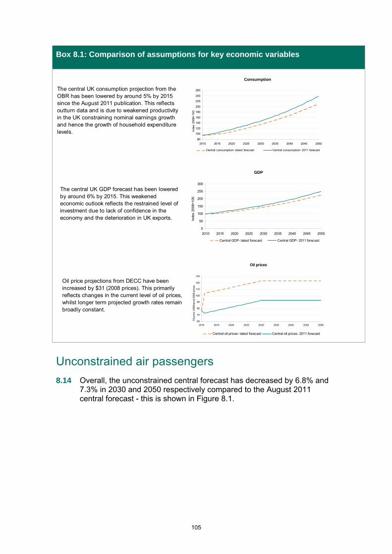
Box 8.1: Comparison of assumptions for key economic variables
Consumption
80
100
120
140
160
180
200
220
240
260
2010 2015 2020 2025 2030 2035 2040 2045 2050
Inde
x 20
08=
100
Central consumption- latest forecast Central consumption- 2011 forecast
GDP
0
50
100
150
200
250
300
2010 2015 2020 2025 2030 2035 2040 2045 2050
Inde
x 20
08=
100
Central GDP- latest forecast Central GDP- 2011 forecast
Oil prices
60
70
80
90
100
110
120
130
2010 2015 2020 2025 2030 2035 2040 2045 2050
Oil
pric
e U
S$/
barr
el 2
008
pric
es
Central oil prices- latest forecast Central oil prices- 2011 forecast
The central UK consumption projection from the OBR has been lowered by around 5% by 2015 since the August 2011 publication. This reflects outturn data and is due to weakened productivityin the UK constraining nominal earnings growth and hence the growth of household expenditure levels.
The central UK GDP forecast has been lowered by around 6% by 2015. This weakened economic outlook reflects the restrained level of investment due to lack of confidence in the economy and the deterioration in UK exports.
Oil price projections from DECC have been increased by $31 (2008 prices). This primarily reflects changes in the current level of oil prices, whilst longer term projected growth rates remain broadly constant.
Unconstrained air passengers
8.14 Overall, the unconstrained central forecast has decreased by 6.8% and 7.3% in 2030 and 2050 respectively compared to the August 2011 central forecast - this is shown in Figure 8.1.
105

Figure 8.1: Change in unconstrained national air passenger forecasts
8.15 Figure 8.2 explains this change in central forecasts compared to the 2011 publication in terms of the contributions of each of the updated inputs, expressed as a percentage of the total overall change for that year.
Figure 8.2: Impact of input changes on passenger forecasts
2012 outturn passengers
Exchange rates
Carbon prices
Oil prices Foreign GDPUK GDP and
consumptionFleet
efficiency
-80%
-70%
-60%
-50%
-40%
-30%
-20%
-10%
0%
10%
Ch
an
ge
in p
ax
as
a p
erc
en
tag
e o
f to
tal c
ha
ng
e
2030 2050
Effects attributed to changes in APD and airline costs are negligible.
8.16 The decrease in forecast passenger numbers since 2011’s central forecast can be largely explained by the change in projections of UK
106

GDP and consumer expenditure. They account for more than 60% of the drop in demand forecast.
8.17 Similarly, lower projections of foreign GDP due to slower-than-expected economic recovery have also pushed passenger demand forecasts downwards in the near term. Another significant factor driving down the latest passenger forecasts compared to the last publication is the change in oil price assumptions. Higher oil price projections are expected to push up future air fares relative to the projection of air fares used in the 2011 forecasts, resulting in lower passenger demand forecasts.
8.18 After taking all the revised inputs into account, the model projected passenger numbers for 2012 to be around 3 million (2%) lower than outturn passenger data from the CAA indicated.98 The forecast was adjusted upwards to reflect this difference, represented in Figure 8.2 by the “2012 Outturn passengers” category.
Constrained passengers
8.19 Overall, the constrained passenger numbers are around 6% lower in 2030 and 4% lower in 2050 in the central constrained forecast, as summarised by Table 8.3.
8.20 The changes in constrained forecasts may not be proportionate to changes in unconstrained forecasts as the level and geographic balance of demand and the changes made to the definition of the 'maximum use' capacity scenario will alter which airports reach capacity and how future passengers react.
Table 8.3: Change in constrained air passenger forecasts
2011 forecast
Latest forecast
2011 forecast
Latest forecast
2011 forecast
Latest forecast
2030 298 276 334 313 381 3472050 381 339 471 447
National Air Passenger Allocation Model failed to reach 2050.
Low Central High
98 An estimate for 2012 passenger numbers was made based on the 11 months of outturn data available at the time.
107

Constrained ATMs
8.21 Figure 8.3 compares the constrained forecasts of ATMs between 2011 and the latest forecasts. The latest central forecast has gone down by 8.1% in 2030 and by 5.2% in 2050.
Figure 8.3: Change in constrained ATM forecasts
Airport use
8.22 Table 8.2 below summarises changes in constrained passenger forecasts for the largest airports between the 2011 and these latest forecasts. In comparison with the 2011 central forecast, the number of passengers travelling via London airports has increased while demand in other regions has fallen. This is largely driven by three factors.
Aligning the model with 2011 outturn passenger data from the CAA suggested that a greater proportion of demand was using airports in the South East than was projected in the 2011 forecasts. This largely explains the reduction in passenger numbers in Scottish and northern airports.
The change in airport capacity assumptions discussed in paragraph 8.7 has marginally increased capacity at Gatwick and Luton airports. This also helps explain some of the other airport level results, for example, the fall in passenger numbers in East Midlands Airport and the rise in passengers at Birmingham Airport in the later years can be explained by the changes in airport capacity assumptions after 2030.
The introduction of Southend Airport into the model and the higher capacity assumption for Gatwick have lowered congestion costs at
108

South East airports in the central case and this reduces the level of spill to airports such as Birmingham in the medium term.
Table 8.4: Change in airport use, 2011 and current forecast
mppa2011 Central
ForecastCurrent
Forecast2011 Central
ForecastCurrent
Forecast
Heathrow 85 82 86 93Gatwick 39 41 41 44Stansted 34 36 32 35Luton 17 18 16 18London City 7 6 7 7London 181 183 183 197
Manchester 35 28 55 55Birmingham 26 17 27 38Glasgow 10 9 19 12Edinburgh 16 13 20 20Bristol 9 10 12 12Newcastle 6 5 10 9Belfast International 8 7 11 10Liverpool 6 7 19 15East Midlands 4 4 25 14*Other modelled 32 30 88 65
Total 334 313 470 448
* includes Southend airport in current forecast
2030 2050
109

CO2 emissions
8.23 Central CO2 emission projections are around 9% lower in 2030 and 4% lower in 2050 compared to the August 2011 forecasts. This reflects both the changes in the numbers of ATMs and latest outturn emissions data. Figure 8.4 shows the changes in more detail.
Figure 8.4: CO2 emissions compared to August 2011 forecast
110

9. Model performance
Performance of the model over recent years
9.1 The econometric models resulting from the estimation process show a strong ability to fit the historic data up to the time series model baseline of 2008. Figure 9.1 shows that, when aggregated to the national level, the models accurately predict the trend in passenger demand, while also capturing many shorter term movements. Annex A provides details of the performance of the individual models used for each of the 19 market sectors.
Figure 9.1: Actual and fitted UK terminal passengers 1996-2008
100
120
140
160
180
200
220
240
260
1996 1998 2000 2002 2004 2006 2008
UK
ter
min
al p
asse
nger
s m
ppa
Model Fit Actual
Note: not every model is fitted to data prior to 1996, so totals consistent with CAA outturn data can be presented from
1996 only.
9.2 As the latest version of the model begins forecasting from 2008, it can be used to produce 'predictions' for 2009, 2010, 2011 and 2012 using outturn values for all the driving variables included in the models (i.e. GDP, oil prices, APD etc). Table 9.1 shows the difference between these predictions and outturn passenger numbers for those years.
111

Table 9.1: Difference between outturn data and NAPDM predictions 2009-2012
2009 2010 2011 2012
Percentage difference from outturn data
+ 3% + 14% + 4% + 2%
9.3 Table 9.1 demonstrates that the predictions of UK air passengers exceed the outturn statistics for the numbers of passengers using UK airports between 2009 and 2012. There is a particularly high difference in 2010, the year of the main Eyjafjallajökul volcanic ash episode. This mismatch appears to be temporary with the differences returning to relatively small levels by 2012 and having little effect on the future projections. Much of the over-forecast is concentrated in the domestic and international business markets. The reasons for this could include:
further structural changes in the domestic aviation air market;
sectors of UK business activities with high propensity to fly such as the financial sector having been disproportionately hit compared to other areas, an effect not fully captured by overall UK GDP; and,
the volcanic ash episode of May-June 2010 cannot be accounted for in the model predictions and resulted in an estimated 4.8m lost terminal passengers.
9.4 In producing the updated forecasts the national unconstrained forecasts for 2009, 2010, 2011 and 2012 produced by the National Air Passenger Demand Model, have been adjusted to equal the observed number of UK terminal passengers in those years. Forecasts for future years have been adjusted in line with the difference observed in 2012 in order to ensure that any un-modelled structural changes in the aviation market are reflected in the forecasts.
Validation of airport, route and ATM forecasts
9.5 An important factor determining the confidence that can be placed in a calibrated model is its ability to replicate independent observed data. The process of comparing modelled or 'predicted' output against independent 'actual' or observed data is known as 'validation'. In the passenger to airport allocation model, this assessment is undertaken at various levels of detail:
overall airport throughput (passengers and aircraft)
passengers and aircraft travelling between individual airports and destination areas (zones);
loadings on aircraft; and
numbers of specific routes operating at individual airports.
112

9.6 These assessments are an important part of the quality assurance of the forecast results.
9.7 Obtaining full sets of passenger demand for all UK passengers from CAA interviews and statistics is an onerous task. The initial passenger demand and supply networks (the airports and the routes they offer) are input for 2008 as was the case with the last forecast publication of 2011. However, the validation exercise has been moved forward from 2009 to 2011. It is now calibrated to the most recent year for which the full CAA statistical returns data are available. This CAA data is used as the independent check data (the "actual" heading in the tables below).
9.8 Validating to a base year of 2011 improves the quality of the model forecasts, but is a more severe test of model performance because:
the model is required to forecast through 2008, 2009 and 2010 prior to reaching the validation year and in each year after the 2008 base the numbers of aircraft and loadings on each route are calculated internally by the model in response to modelled passengers rather than using the input base year supply data; and
demand in 2011 has been created by applying the regional growth factors from 2008 so modelled demand will not necessarily match actual demand and will also be subject to local variation that has taken place since the base year.
113

Airport level passenger validation
9.9 Table 9.2 below reports the accuracy of the model in predicting passenger demand at the London airports and those airports that handled more than 3mppa in 2011 (in total these comprise 92% of modelled demand). It shows that the model is very successful in predicting the number of passengers travelling through each UK airport. Demand is predicted to within +/-1% at Heathrow and Stansted and for the London airports as a group. The London area total fitted value is highly accurate. At all the larger airports outside the London area the model is accurate to within +/-10%. The national total for all 31 airports in the model is also highly accurate. More detailed analysis of the model’s calibration and validation at all airports is set out in Annex B.
Table 9.2: Actual and predicted passengers at modelled airports, mppa in 2011
Actual Fitted Difference Difference (%)Heathrow 69.4 69.5 0.1 0%Gatwick 33.6 35.1 1.4 4%Stansted 18.0 17.9 -0.1 -1%Luton 9.5 10.2 0.7 7%London City 3.0 2.9 -0.1 -3%London subtotal 133.6 135.5 1.9 1%Manchester 18.8 19.8 1.0 5%Birmingham 8.6 9.0 0.4 4%Glasgow 6.9 6.3 -0.6 -9%Edinburgh 9.4 8.8 -0.6 -6%Bristol 5.8 5.8 0.0 0%Newcastle 4.3 4.0 -0.3 -7%Belfast International 4.1 4.0 -0.1 -2%Liverpool 5.2 5.1 -0.1 -2%East Midlands 4.2 3.9 -0.4 -8%Other airports in model 16.8 16.7 -0.2 -1%Total in model 217.7 218.9 1.1 1%Other non-modelled airports 2.3National total 220.1
114

Route group zone level passenger validation
9.10 Table 9.3 summarises the model's success in predicting passenger demand on individual routes or routes grouped into model zones at each airport. The table presents the validation against data for the 697 modelled routes99 which each carried more than 25,000 passengers a year in 2011.100 The results are weighted by the number of passengers on each route. The table shows that two thirds of the passengers are on routes where passenger numbers are predicted to within +/-10% of actual figures, rising to over 80% within +/-20%. Of the 4% of passengers travelling on routes in the 50%+ error band, a disproportionately large share, almost half, were on smaller internal domestic services or inclusive tour charter routes.
Table 9.3: Zone level passenger prediction, 2011, all flights (domestic and international)
Error band
Proportion of passengers on routes in
band
Cumulative proportion
0%-5% 47% 47%5%-10% 20% 66%
10%-20% 16% 82%20%-30% 8% 90%30%-40% 5% 95%40%-50% 2% 96%
50%+ 4% 100%
9.11 Figure 9.2 illustrates the correlation between the actual and fitted passenger numbers in a scatter plot. The trend line has a slope close to one, and the data are scattered very closely around the trend line. This indicates that the model is very successful in predicting route level demands in the base year. Annex B provides more detailed validation results.101
99 The model has 59 specific airport destinations in the UK and Europe and 21 destinations which are geographical groupings of routes to smaller or more remote airports (a "route group"). Strictly the definition of route here is "route or route group". 100 Validation in practice extended to all routes with more than 5,000 passengers in 2009, extending the total calibration exercise to include close to 1,000 separate routes. 101 A more detailed split into domestic and international passengers is available in Annex B.
115

Figure 9.2: Scatter plot of actual and fitted passenger numbers by route, all flights (domestic and international), 2011
y = 0.9888x + 61.46
R2 = 0.9894
0
1
2
3
4
5
6
7
8
9
10
0 1 2 3 4 5 6 7 8 9 10
mod
elle
d m
ppa
observed mppa
116

Airport level ATM validation
9.12 As with the model of passengers' airport choice, an important factor determining the confidence which can be placed in this calibrated model is its ability to replicate observed data on numbers of passenger ATMs and their loadings at each airport and on each route. The model’s ability to successfully predict 2011 ATM demand has therefore been examined at both the airport and route level.
9.13 Table 9.4 below reports actual and predicted ATMs at the London airports and those regional airports with over 3mppa demand (these comprise 92% of passenger demand). It shows that the model predicts ATMs accurately at London area airports. At Heathrow and Stansted, ATMs are predicted to within +/-2% and only the smallest airport, London City is outside +/-5%. Total London area passenger aircraft traffic is accurately forecast to within +/-2%.
9.14 The ATM predictions at the larger airports outside the London area are similarly accurate, with one exception, all being within +/-15% of actual figures. Annex B sets out the ATM results for all modelled UK airports.
Table 9.4: Actual and predicted ATMs at modelled airports, 000s per annum in 2011
2011 Fitted Difference Difference (%)Heathrow 477 488 11.2 2%Gatwick 245 257 11.8 5%Stansted 139 150 11.7 8%Luton 76 81 4.5 6%London City 67 61 -6.1 -9%London subtotal 1,004 1,037 33.1 3%Manchester 158 166 8.1 5%Birmingham 85 92 7.7 9%Glasgow 72 66 -6.0 -8%Edinburgh 109 98 -11.0 -10%Bristol 53 53 0.5 1%Newcastle 45 43 -2.5 -5%Belfast International 38 42 4.0 10%Liverpool 46 43 -3.2 -7%East Midlands 58 50 -8.8 -15%Other airports in model 341 322 -19.5 -6%Total in model 2,010 2,013 2.3 0.1%Other non-modelled airports 132National total 2,143
117

Route group zone level ATM validation
9.15 Table 9.5 shows the performance of the model in predicting aircraft movements by international geographic zone.102 As with the passenger demand predictions, the large number of routes means the results are summarised by accuracy band.
9.16 The validation of aircraft movements by route is a particularly stringent test of the model accuracy, being dependent on both the modelled passenger allocation to the route and the performance of the ATM forecasting model in allocating appropriate aircraft sizes and types to each route. It also requires that the model satisfactorily predicts aircraft loads (passengers per ATM) at the route level and, as explained in paragraph 9.7, reflects the cumulative effect of 3 years of ATM calculations since the model base year of 2008.
9.17 Table 9.5 shows that about 51% of routes have ATMs predicted to within +/-20%. Of the 17% of passengers travelling on ATMs in routes in the 50%+ error band, over half were on smaller internal domestic services or inclusive tour charter routes.
Table 9.5: Route level passenger prediction, 2011, all flights (domestic and international)
Error bandRoutes in
bandCumulative proportion
0%-5% 15% 15%5%-10% 12% 27%
10%-20% 24% 51%20%-30% 15% 66%30%-40% 10% 76%40%-50% 7% 83%
50%+ 17% 100%
9.18 Figure 9.3 shows the correlation between actual and fitted ATMs by route. The slope of the trend line being close to one, the low intercept, and the fairly tight fit of the data around the trend line indicate that the model is successful in predicting base year ATMs by route.
102 Route here is used in the sense of the 48 international model destination zones including the route group zones, but not the separate destinations within the grouped zones.
118

Figure 9.3: Scatter plot of actual and fitted passenger numbers by route, all flights (domestic and international), 2011
y = 1.009x + 7.0412
R2 = 0.9618
0
10,000
20,000
30,000
40,000
50,000
60,000
0 10,000 20,000 30,000 40,000 50,000
observed ATMs
mod
elle
d A
TM
s
Destinations
9.19 Paragraphs 9.10-9.11 reported the model performance in assigning passengers between UK airports and destination zones. In the model definition (see paragraphs 2.35-2.37 in chapter 2) the 21 largest European airports in terms of UK traffic are discretely modelled as separate zones. However, all the long haul airports and the rest of the European airports are members of 27 "route group" zones. The passenger to airport allocation model analyses the level of demand between a UK airport and a "route group zone" to forecast how many members of the route group zone are served by a particular UK airport. The quality of this aspect of model performance is important in three key respects:
it determines the numbers of aircraft movements to a route group;
it determines the modelled aircraft sizes to different zones and allows a mix of different aircraft sizes to the different destinations within the route group; and
it provides a more meaningful measure of connectivity at specific UK airports.
9.20 The first two attributes impact on frequency and have an impact on the allocation of passengers to routes, the forecasting of numbers of aircraft movements and the validation reported above. However, it is the third aspect that is particularly relevant when using the model as an indicator of future UK connectivity. An additional base year validation against actuals exercise has therefore been undertaken on this aspect of model
119

performance to establish the suitability of the model for forecasting and quantifying future UK connectivity.
Table 9.6: Actual and predicted numbers of international destinations served (scheduled services only)
2011 Actual 2011 Modelled DifferenceHeathrow 175 174 -1Gatwick 214 232 18Stansted 148 146 -2Luton 89 101 12London City 31 26 -5London subtotal 657 679 22Manchester 142 145 3Birmingham 79 79 0Glasgow 32 20 -12Edinburgh 76 76 0Bristol 70 69 -1Newcastle 36 33 -3Belfast International 28 30 2Liverpool 65 69 4East Midlands 59 50 -9Other airports in model 171 177 6Total in model 1,415 1,427 12* Destination only counted if more than 5000 passengers per year
9.21 Table 9.6 compares actual full service and low cost scheduled routes at each airport in 2011 with those predicted by the model. Only routes with more than 5,000 passengers a year are included, but flows below this level will represent considerably less than 1 return flight a year at any UK airport.103
9.22 There is an equally robust correspondence between actual and predicted destinations served for international charter flights. Figure 9.4 shows this information in the form of a scatter plot for the 31 modelled airports (again for routes with more 5,000 passengers a year) and includes charter destinations in the analysis. The slope of the trend line is close to one and the low intercept confirms the good representation of actual route numbers by the model in 2011.
9.23 More data on the forecasting of destinations and connectivity is given in Annex B. This includes analysis of all airports in the model, separate scheduled and charter connectivity analysis and the numbers of UK routes at each of the foreign destination zones.
103 The table adds the model's 'full service' and low cost scheduled sectors,. So if the same destination is served by both a low cost and full service carrier at the same airport it will be counted twice at that airport. Equivalent tables for each sector which remove this potential effect are included in Annex B.
120

Figure 9.4: Scatter plot of actual and fitted international destinations served at UK airports (all flight types)
y = 1.077x - 4.4869R2 = 0.9935
-50
0
50
100
150
200
250
300
350
0 50 100 150 200 250 300 350
Modelled routes
Act
ual r
oute
s
121

Annex A: Econometric models in the National Air Passenger Demand Model
A.1 This annex provides a technical overview of the data and methods on which the econometric models used in the National Air Passenger Demand Model are based, plus the resulting parameter estimates, diagnostic tests and key long run elasticities.
A.2 The econometric models used were re-estimated prior to the publication of UK Aviation Forecasts, 2011.104 Annex A of the 2011 publication as well as two technical notes published alongside that report provide more detailed descriptions of the changes made and the data used.105
A.3 Ultimately the aim of the econometric analysis was to estimate models which successfully explained past demand movements, had parameter estimates in line with economic theory, and passed the standard diagnostic tests. Particular emphasis was placed on establishing the relationship between demand and income variables, and searching for fare effects where data permitted. Passengers are segmented into separate markets that are expected to have broadly similar characteristics. The 19 market segments are, therefore, split according to:
the global region a passenger is travelling to or from;
whether the passenger is a UK or overseas resident;
the passenger's journey purpose (business or leisure);
the type of flight the passenger is on (international or domestic); and,
whether the passenger is making an international to international connection using a UK airport.
104 https://www.gov.uk/government/publications/uk-aviation-forecasts-2011 105 ‘Re-estimating the National Air Passenger Demand Model Econometric Equations, DfT 2011’ ‘Reflecting changes in the relationship between UK air travel and its key drivers in the National Air Passenger Demand Model’, DfT, 2011
122
Data sources
A.4 The primary source of data for air passenger demand and fares paid is the ONS International Passenger Survey (IPS). This survey dataset gives a continuous time series for traffic from 1984-2008, and for fares from 1987-2008. However, it collects fare data from only UK passengers, and does not include domestic air passengers.
A.5 The passenger interview surveys conducted by the CAA provide an important supplementary source which has been used to supply time series for international-to-international interlining passengers, to provide information on journey purpose (business/leisure) and the share of domestic interliner passengers on domestic routes. The survey results also provide some data on domestic air fares and fares paid by foreign passengers as well as providing an independent validation of the IPS fares data for 1982 to 1987 which was compiled in the form of an index from an earlier DfT forecasting exercise.106
A.6 Elsewhere ONS data is used for UK GDP and consumer expenditure, UN statistics on foreign GDP, HM Revenue & Customs for trade data, Bank of England quarterly returns for dollar exchange rates, and UN local currency GDP statistics for other currency to dollar exchange rates.
Econometric methods
A.7 Most of the markets display strongly trended variables. There are upward trends in traffic, but also in independent variables such as GDP, exports and imports. Similarly there is typically a downwards trend in air fares. These trends are non-stationary.107
A.8 Using standard regression techniques with non-stationary time series data can result in spurious regressions, because the standard errors on the estimated parameters are biased, leading to measures of parameter significance and model goodness of fit that are misleadingly high. If the data series are non stationary but a linear combination of them is stationary (their time paths are linked), then the series are said to be cointegrated - this means that there is a meaningful relationship between them.108
A.9 This forecast adopts a series of Unrestricted Error Correction Models (UECM) to model passenger numbers in each market segment. A number of other techniques were considered, however, it was found that the UECM approach offered the best balance between data
106 Air Passenger Forecasts for the United Kingdom’, Department for Environment Transport and the Regions, 2000 107 i.e. they are not following fixed, constant time trends. 108 To be cointegrated the variables must be integrated of the same order - this is the minimum number of differences required to obtain a stationary series.
123

requirements and estimation efficiency.109 Cointegration was tested for using the augmented Dickey-Fuller test on the residuals of the long-run form of the relationship.110 A number of different functional forms were tested but the log-log form, where all variables are expressed in natural logarithms, was chosen for all models as it was able to best explain past movements in air passenger traffic.
A.10 The general form of the relationship is described below:
Technical Peer Review
A.11 Expert academic advice was sought to ensure the methods used to re-estimate the models were suitable. A team at the University of Westminster (UoW), led by Professor Austin Smyth, evaluated the techniques and subsequently ad hoc advice was also provided by Professor Joyce Dargay, Emeritus Professor of Transport Econometrics at the Institute of Transport Studies. Professor Dargay examined all of the final models and endorsed the methods used, as well as making some useful suggestions as to how to interpret the findings.
Econometric models used in the NAPDM
Parameter estimates and diagnostics
A.12 The results of the econometric analysis of each of the 19 passenger markets used in the NAPDM are summarised in the following tables. Table A1 reports the parameter estimates and Table A2 reports the t-statistics.
A.13 Each of the 19 passenger markets is described by a typically three letter code used to identify nationality, purpose and the region of the journey:
109 A full explanation of these methods can be found in Applied Time Series Econometrics, W.Enders, 2004, Wiley, 2nd ed. pp 335-339 110 This is the test used in the first step of the Engle-Granger approach. If the null hypothesis of non-stationarity of the residuals can be rejected then there is evidence of a cointegrated relationship.
124

Journeys between the UK and foreign countries:
First letter denotes UK resident (U), or Foreign resident (F).
Second letter denotes Business (B), or Leisure (L).
Third letter denotes foreign origin or destination: W: Western Europe; O:
OECD excluding Western Europe; N: Newly Industrialised Countries
(NICs); L: Less Developed Countries (LDCs).
Domestic journeys within the UK: DMB: Domestic business; DML:
Domestic leisure.
International to international (interliner) passengers: I-I.
A.14 Thus the codes used for the nineteen market sectors in the following tables are:
UBW UK resident, business, Western Europe
UBO UK resident, business, OECD
UBN UK resident, business, NIC
UBL UK resident, business, LDC
ULW UK resident, leisure, Western Europe
ULO UK resident, leisure, OECD
ULN UK resident, leisure, NIC
ULL UK resident, leisure, LDC
FBW Foreign resident, business, Western Europe
FBO Foreign resident, business, OECD
FBN Foreign resident, business, NIC
FBL Foreign resident, business, LDC
FLW Foreign resident, leisure, Western Europe
FLO Foreign resident, leisure, OECD
FLN Foreign resident, leisure, NIC
FLL Foreign resident, leisure, LDC
DMB Domestic, business
DML Domestic, leisure
I to I International-international interliner (non-UK transfer)
125

A.15 The notation used for the column headings in Table A1 and Table A2 is:
lntra Natural logarithm of Traffic levels
lngdp Natural logarithm of UK GDP
lncon Natural logarithm of UK Consumption
lnfgp Natural logarithm of Foreign GDP
lnips Natural logarithm of UK Passenger Fares
lnpfr Natural logarithm of Foreign Passenger Fares
lnexr Natural logarithm of UK Nominal Exchange Rate
lnimp Natural logarithm of UK Imports
lnexp Natural logarithm of UK Exports
d.[variable] Differenced variable
l.[variable] or L1 Lagged variable (one year)
d.l.[variable] or DL Differenced lagged (one year) variable
D[year] Dummy
A.16 Various diagnostic tests have been completed to check that the estimated equations are robust. Plots of fitted versus actual were studied as a first check of accuracy, followed by a test for omitted variables (Ramsay RESET), a test for heteroskedasticity (Breusch-Pagan), and a test for autocorrelation (Breusch-Godfrey). The results of these tests for each passenger market can be found in Table A3. Table A3 also shows the 2008 share of total modelled passenger traffic to and from the UK.
A.17 Tables A1 to A3 show that:
in all markets an R2 value111 exceeding 0.6 is obtained;
the income variables are significant at the 5% level or higher in all but the FBN and I-I models, where the foreign GDP variable is significant at the 10% level in I-I and insignificant in the FBN model. The fare level variables are significant at the 5% level, with two exceptions (FLN and FBO), where the variable is retained because the variables are jointly significant, the parameter is of the correct sign and magnitude, and therefore likely to be useful in forecasting,112 and
111 R2 is a measure of the goodness of fit of a model. It measures the proportion of variability of the dependent variable (the number of air passengers) in the past that is explained by the model. 112 The critical values for the t-stats, given the 24 observations in the UK and foreign market models (excluding domestic and I-I markets), are 1.71 at the 10% level, 2.06 at the 5% level and 2.80 at the 1% level. Given that there are 19 observations in the domestic models the critical values for the t-stats are 1.73 at the 10% level, 2.09 at the 5% level and 2.86 at the 1% level. The critical values for the t-stat in the I-I model, given 12 observations, are 1.78 at the 10% level, 2.18 at the 5% level and 3.05 at the 1% level.
126

127
there is no evidence of autocorrelation or heteroscedasticity at the 5% level except in the UK Business to Western Europe market – which suffers from autocorrelation.
A.18 In estimating the econometric models a constant was initially included in every model. The constant was only excluded if it was found to be statistically insignificant.

128
Table A1: Parameter estimates
Sector
UBW D-Lnt-Tra 0 1.27 -0.35 0.47 -0.78 0.57 -0.21 0.42
UBO D-Lnt-Tra 0 2.40 0.02 -0.41 0.18 0.21
UBN D-Lnt-Tra 0 4.98 0.54 -0.86 0.41 0.46
UBL D-Lnt-Tra 0 4.98 0.54 -0.86 0.41 0.46
ULW D-Lnt-Tra 0 2.82 -0.47 0.62 -0.16 0.13
ULO D-Lnt-Tra 0 -0.85 0.81 -0.73 0.56 -0.25 0.43
ULN D-Lnt-Tra 0 1.88 -0.16 -0.84 1.34 -0.46
ULL D-Lnt-Tra 0 2.60 -0.49 -0.51 0.95 -0.44
FBW D-Lnt-Tra 0.79 1.87 0.52 -1.21 0.75 -0.30 0.60 -0.15
FBO D-Lnt-Tra 2.95 -0.45 0.67 -1.02 -0.17 0.57
FBN D-Lnt-Tra 0.49 0.53 -0.30 0.23 0.64
FBL D-Lnt-Tra 0.54 0.18 -0.39 0.27 0.52
FLW D-Lnt-Tra 0.94 -0.67 -0.36 0.44 -0.27 -0.08 -0.21
FLO D-Lnt-Tra 8.90 0.94 -0.20 -0.75 0.41 -1.58
FLN D-Lnt-Tra 3.74 0.20 -0.18 -1.02 0.53 -0.22 -0.28
FLL D-Lnt-Tra 2.10 0.08 0.003 -0.53 0.25 -0.18 0.44 -0.24
DMB D-Lnt-Tra 0 2.96 -0.41 0.41
DML D-Lnt-Tra -2.42 2.41 -0.42 0.95 -0.08
I to I D-Lnt-Tra 5.82 0.06 -0.24 -1.06 0.50 -0.70 -0.15
d9
6
0.26
0.26
d.l
ng
dp
d.l
nco
n
d.l
nfg
p
l.ln
imp
I.In
exr
d9
1
l.ln
exp
l.ln
fgp
d9
3
d0
0
d0
1
d0
2
d0
3
d.l
nim
p
l.ln
tra
l.ln
ips
l.ln
pfr
VariableC
on
st
De
p V
ari
ab
le
-0.20
l.ln
gd
p
l.ln
co
n
d.l
nip
s
d.l
np
fr
d.l
nex
r
d.l
nex
p

129
Table A2: Parameter t-statistics
UBW D-Lnt-Tra 0 2.05 -1.93 4.14 -3.65 3.23 -3.17 3.39 0.00 0.00 0.00 0.00 0.00 0.00
UBO D-Lnt-Tra 0 6.26 0.19 -6.89 3.52 3.92 0.00 0.00 0.00 0.00 0.00 0.00
UBN D-Lnt-Tra 0 3.31 2.32 -5.09 4.63 4.42
UBL D-Lnt-Tra 3.31 2.32 -5.09 4.63 4.42
ULW D-Lnt-Tra 0 4.29 -2.90 2.91 -2.79 -2.56
ULO D-Lnt-Tra 0 -2.26 3.88 -3.35 2.78 -2.84 2.51
ULN D-Lnt-Tra 0 2.02 -0.79 -3.46 3.29 -2.98
ULL D-Lnt-Tra 0 2.62 -2.33 -2.44 2.37 -2.28 2.86
FBW D-Lnt-Tra 1.10 3.70 3.70 -8.60 5.00 -3.50 6.90 -3.35
FBO D-Lnt-Tra 2.30 -1.50 3.60 -4.10 -0.90 3.60
FBN D-Lnt-Tra 2.00 2.20 -1.90 1.60 5.21 -4.98FBL D-Lnt-Tra 2.40 1.60 -3.80 4.30 7.71
FLW D-Lnt-Tra 1.10 -3.70 -5.50 2.70 -2.80 -1.61 -4.45
FLO D-Lnt-Tra 2.80 2.40 -0.20 -4.40 2.50 -2.50
FLN D-Lnt-Tra 2.70 0.50 -0.40 -4.50 3.60 -1.10 -2.18 -3.07
FLL D-Lnt-Tra 2.30 0.80 -4.30 3.20 -2.20 6 -3.53
DMB D-Lnt-Tra 0 4.50 -3.48 3.42 3.39
DML D-Lnt-Tra -2.42 4.86 -2.34 2.27 -2.2
I to I D-Lnt-Tra 3.40 0.10 -1.00 -5.80 2.00 -3.40 -4.73
-3.02
Sector
VariableC
on
st
d.l
ng
dp
d.l
nco
n
d.l
nfg
p
d.l
nip
s
d.l
np
fr
d.l
nex
r
d.l
nex
p
d.l
nim
p
l.ln
tra
l.ln
gd
p
l.ln
co
n
l.ln
fgp
l.ln
ips
l.ln
pfr
l.ln
ex
p
l.ln
imp
d08
I.In
ex
r
d91
d93
d00
3.76
Dep
Var
iab
le
d01
d02
d96
3.76
d03
d04
d05

Table A3: Results of diagnostic tests
UBW 6% 0.78 8.6 0 5.94 0.01 5 0.02 0.05 0.82
UBO 1% 0.89 30.22 0 0.76 0.38 1.04 0.4 0.23 0.63
UBN 0% 0.79 11.01 0 0.36 0.55 0.4 0.75 0.14 0.71
UBL 1% 0.79 11.01 0 0.36 0.55 0.4 0.75 0.14 0.71
ULW 33% 0.73 10.06 0 0.11 0.74 1.7 0.21 0.23 0.64
ULO 5% 0.7 6.89 0.001 0.5 0.48 0.88 0.47 0.04 0.85
ULN 1% 0.7 8.66 0 0.89 0.35 3.15 0.06 1.35 0.25
ULL 6% 0.79 10.95 0 0.14 0.7 0.33 0.81 0.22 0.64
FBW 5% 0.87 14.85 0 1.14 0.29 3.53 0.05 0.75 0.39
FBO 1% 0.6 5.4 0.003 0.14 0.71 0.66 0.59 1.28 0.26
FBN 0% 0.84 18.44 0 2.41 0.12 0.35 0.71 0.29 0.59
FBL 1% 0.83 23.1 0 3.11 0.08 0.52 0.68 0.33 0.56
FLW 10% 0.82 12.84 0 2.5 0.11 0.88 0.48 1.58 0.21
FLO 3% 0.63 4.91 0.004 4.02 0.05 0.5 0.69 0.66 0.41
FLN 0% 0.7 5.28 0.003 3.04 0.08 1.25 0.33 1.46 0.23
FLL 1% 0.85 13.44 0 0.02 0.89 2.14 0.14 0.96 0.33
DMB 7% 0.75 11.19 0 1.19 0.28 0.74 0.55 0.18 0.67
DML 8% 0.66 6.88 0.003 2.09 0.15 1.58 0.25 0.29 0.59
I to I 10% 0.96 22.8 0.002 0.11 0.74 0.61 0.67 0.02 0.9
RE
SE
T
sign
ificanc
e
Breu
sch-P
agan
h
eterosk
edasticity
Breu
sch-P
agan
sig
nifican
ceF sig
Breu
sch
-G
od
frey au
toco
rrelatio
n
Breu
sch
-G
od
frey sig
nifican
ce
Ram
sey R
ES
ETSector
2008 share of modelled
traffic R2 F
130

Long run air fare and income elasticities
A.19 Price and income elasticities have been calculated (where possible) using the method in Figure A1.
Figure A1: Calculation of price and income elasticities
Given an ECM equation with traffic and fares variables expressed in natural logarithms (simplified):
)ln(lnlnln 11 faredfaretratrad tt
Fare elasticity of demand with respect to traffic can be derived. Assuming that in the long run equilibrium, d lntra and d lnfare are zero:
11
11
11
lnln
lnln
lnln0
tt
tt
tt
faretra
faretra
faretra
Now each side can be differentiated and rearranged to find that the fare elasticity of demand is given by (-):
1
1
1
1
11
11
/1
t
t
t
t
tt
tt
tra
fare
dfare
dtra
dfarefare
dtratra
A.20 The measurement of income elasticities was complicated in some markets by the presence of more than one income variable. This was primarily an issue in business markets where it was found, not unexpectedly, that demand was driven by economic activity in the UK and in the overseas market. This was dealt with by taking the sum of the coefficients on these components and dividing through by the (negative of the) coefficient on lagged traffic (α in Figure A1) to find the income elasticity.
A.21 Another complication in calculating income elasticities concerned the foreign leisure market to Western Europe which contained UK consumer spending as its only income variable. In this market the coefficient on UK consumer spending was used to calculate the income elasticity on the basis that UK consumer spending is treated as operating as a proxy for consumer spending in the rest of Europe.
A.22 There are a few markets where it was suspected that model or data limitations led to unexpected values for the income elasticities (YEDs) and price elasticities (PEDs). In these circumstances, it is reasonable, for the purposes of forecasting, to impose YEDs or PEDs if there is a strong rationale for believing a certain relationship exists which, because of data limitations, has not been picked up in the estimated equations.
131

A.23 This led to imposing PEDs in three markets – ULW, DML, DMB and FLO – and a YED in the DML market:
PED of -0.7 imposed in ULW: The long run PED of -0.33 estimated for the ULW market is likely to be biased downwards because the fare series used reflects scheduled fares only. When we estimated a model for the scheduled market only we find a long run PED of -0.7. This PED is more in line with prior expectations that this would be one of the more price elastic markets. This is because 1) traffic in this segment was dominated by holiday traffic and 2) passengers in this segment are more likely to have alternative modes of transport available to them. The PED of -0.7 is also more consistent with the literature on price elasticities.
PED of -0.33 imposed in FLO: It was not possible to estimate a PED for this model. Based on the expectation that the PED for this market should be of the same order of magnitude as that for ULO (because traveller incomes are broadly similar, there are no realistic alternative travel modes, and FLO passengers tend to have at least as many alternative travel destinations available to them), for forecasting purposes it was decided to impose the PED estimated for the ULO market (-0.33).
PED of -0.3 imposed in DMB: Despite the availability of alternative modes, it was not possible to estimate a PED for this model. Therefore, based on the expectation that the PED market should be of the same order of magnitude as that estimated for the UBW market, for forecasting purposes it was decided to impose the PED estimated for the UBW market (-0.3)
PED of -0.7 imposed in DML: Surpisingly, given the expectation that it would be one of the more price elastic it was not possible to estimate a PED for this sector. Based on the expectation that the PED for this sector should be of broadly the same order of magnitude as that estimated for the ULW market (because of passengers having similar income levels and availability of alternative modes of travel) for forecasting purposes it was decided to impose the PED estimated for the ULW market (-0.7).
YED of 1.5 imposed in DML in 2010: It is considered that the long run YED of 2.3 for the DML market is likely to be an overestimate, and potentially biased because of the omission of a fares variable from the estimated model. It was therefore decided to impose a lower YED of 1.5 in 2010 to compensate for the imposition of a significant fare variable, and to bring the YED closer to that estimated for the ULW sector.
A.24 In addition it proved impossible to derive a satisfactory model for the UBL market. Therefore, for forecasting, the elasticities estimated for the UBN market have been used, on the basis that this is expected to be the most similar of the other sectors for which models were estimated to the UBL sector. Given that the UBL sector is one of the smallest (accounting for 1% of total UK terminal passengers in 2008), the
132

imposition of the model for UBN will not significantly affect the overall forecasts.
A.25 Table A4 below summarises the resulting long run income and air fare elasticities.
Table A4: Long run price and income elasticities of UK air passenger demand
UBW 6% -0.3 1.3
UBO 1% 0.0 1.0
UBN 0% 0.0 1.0
UBL 1% 0.0 1.0
ULW 33% -0.7 1.3
ULO 5% -0.3 1.3
ULN 1% -0.6 1.6
ULL 6% -0.9 1.9
FBW 5% -0.2 1.1
FBO 1% -0.2 0.6
FBN 0% 0.0 0.8
FBL 1% 0.0 0.7
FLW 10% -0.8 1.2
FLO 3% -0.3 0.5
FLN 0% -0.2 0.5
FLL 1% -0.3 0.5
DMB 7% -0.3 1.0
DML 8% -0.7 1.5
I to I 10% -0.7 -0.7 0.5 0.5
Overall 100% -0.6 1.3
Income variable depends on sectorPrice and income elasticities are point estimatesResults are elasticity of terminal passengers to income or fares
Sector YED
Market YED
1.2-0.2
Sector PED Market PED2008 share of
passenger trafficSector
1.0
1.7-0.5
1.4
1.0
-0.7
-0.2
-0.6
A.26 The average PED across all markets is -0.6 and the overall YED is 1.3. It is intuitive that the overall price elasticity is some way below unity, given that passengers may have options for responding to an increase in price which reduces the cost of their trip without preventing it, such as travelling to a less expensive destination, or by a less expensive class of
133

travel or airline. It is also in keeping with findings for other modes that UK transport demand is relatively price inelastic. Chapter 2 demonstrates that these results are broadly in line with other relevant published studies.
Implementation of market maturity in NAPDM
A.27 As described in Chapter 2, there is reason to believe that the historical relationships identified in the econometric models may change over time reflecting market maturity. For all market segments, the econometric models take the Unrestricted Error Correction Model (UECM) form such that:
ttii
iti
tiii
tiit uXYYXY
1,
211
11,
01,0
Where:
Yt is passenger demand in the market segment at time t
Xi,t is the value of explanatory variable DfT at time t
, DfT,DfT and DfT are parameters to be estimated
A.28 When all the variables are expressed in log form, the long run elasticity of demand with respect to explanatory variable Xi is equal to 1
i
A.29 It was not possible to find a way to vary the elasticities through time, while retaining the UECM form. So the focus has concentrated on the long run relationship between passenger demand and its key drivers implied by the UECM estimated for each market segment. For example, the UECM estimated for the ULN market (UK residents travelling for leisure to/from the NICs) is:
tt tttt t uIPS ConTraIPSCon Tra 11 1 ln 46 . 0 ln33.1ln84.0ln16 . 0 ln88 . 1 ln
Where:
LnTrat is the natural logarithm of the number of passengers in ULN at time t
LnCont is the natural logarithm of UK Consumer Spending at time t
LnIPSt is the natural logarithm of fares at time t
This implies a long run relationship of the form:
tttt uIPSConTra
11 ln84.0
46.0ln
84.0
33.1ln
or,
tttt uIPSConTra ln55.0ln58.1ln
134

A.30 The coefficients on lnCont and lnIPSt can be interpreted as the (constant) income (in this case consumer spending) and fare elasticities of demand respectively. As explained previously, this follows because the model is in log-log form.
A.31 By subtracting lnTrat-1 from lnTrat the long run relationship in differences can be expressed such that:
tttt uIPSConTra ln55.0ln58.1ln
A.32 This model form is attractive as it allows variation of the income and price elasticities of demand (1.58 and -0.55 above) through time, without affecting the relationship between demand and income and fare in previous periods. More details of this approach and the sense checks carried out are available in a technical note published alongside UK Aviation Forecasts, August 2011.113
A.33 Chapter 3 described the approach used in incorporating market maturity into the forecasts. Tables A5 to A7 give additional detail about the assumptions applied in the low, central and high maturity cases.
Table A5: Low growth income elasticities (YEDs) and market maturity adjustments
Sector YED in 2010 YED in 2030 YED in 2080
Year maturity factor is
applied from Year saturation
reached
UBW 1.28 0.83 0.26 2015 2085UBO 0.97 0.81 0.26 2015 2085UBN 1.01 0.95 0.37 2025 2095UBL 1.01 0.95 0.37 2025 2095ULW 1.33 0.83 0.26 2015 2085ULO 1.35 0.83 0.26 2015 2085ULN 1.59 1.06 0.28 2015 2085ULL 1.85 1.06 0.28 2015 2085FBW 1.11 0.83 0.26 2015 2085FBO 0.55 0.48 0.23 2015 2085FBN 0.76 0.72 0.32 2025 2095FBL 0.69 0.65 0.3 2025 2095FLW 1.21 0.83 0.26 2015 2085FLO 0.55 0.47 0.22 2015 2085FLN 0.51 0.49 0.27 2025 2095FLL 0.46 0.45 0.26 2025 2095DMB 0.99 0.78 0.25 2010 2085DML 1.50 0.77 0.2 2010 2080
1) Most mature2) Fairly mature 3) Least mature
113 Reflecting changes in the relationship between UK air travel and its key drivers in the National Air passenger demand model, DfT, July 2011
135

Table A6: Central growth income elasticities (YEDs) and market maturity adjustments
Market YED in 2010 YED in 2030 YED in 2080
Year maturity factor is
applied from
Year saturation reached
UBW 1.28 1.13 0.65 2015 2085UBO 0.97 0.89 0.63 2015 2085UBN 1.01 0.98 0.69 2025 2095UBL 1.01 0.98 0.69 2025 2095ULW 1.33 1.18 0.65 2015 2085ULO 1.35 1.19 0.65 2015 2085ULN 1.59 1.38 0.67 2015 2085ULL 1.85 1.58 0.69 2015 2085FBW 1.11 1.00 0.64 2015 2085FBO 0.55 0.55 0.55 2015 2085FBN 0.76 0.75 0.63 2025 2095FBL 0.69 0.68 0.6 2025 2095FLW 1.21 1.08 0.64 2015 2085FLO 0.55 0.55 0.55 2015 2085FLN 0.51 0.51 0.51 2025 2095FLL 0.46 0.46 0.46 2025 2095DMB 0.99 0.88 0.60 2010 2080DML 1.50 1.24 0.6 2010 2080
1) Most mature2) Fairly mature 3) Least mature
136

Table A7: High growth income elasticities (YEDs) and market maturity adjustments
Sector YED in 2010 YED in 2030 YED in 2080
Year maturity factor is
applied from Year saturation
reached
UBW 1.28 1.22 1.02 2015 2085UBO 0.97 0.97 0.97 2015 2085UBN 1.01 1.28 1.06 2025 2095UBL 1.01 1.28 1.06 2025 2095ULW 1.33 1.26 1.02 2015 2085ULO 1.35 1.27 1.02 2015 2085ULN 1.59 1.46 1.04 2015 2085ULL 1.85 1.67 1.06 2015 2085FBW 1.11 1.09 1.01 2015 2085FBO 0.55 0.55 0.55 2015 2085FBN 0.76 1.28 1.06 2025 2095FBL 0.69 1.28 1.1 2025 2095FLW 1.21 1.16 1.01 2015 2085FLO 0.55 0.55 0.55 2015 2085FLN 0.51 1.28 1.06 2025 2095FLL 0.46 1.28 1.06 2025 2095DMB 0.99 0.99 0.99 2010 2080DML 1.50 1.71 1.0 2010 2080
1) Most mature2) Fairly mature 3) Least mature
137

Annex B: Model validation results
Annex B.1
Airport level: comparison of actual (CAA returns) and modelled passengers and ATMs, 2011
Actual Fitted Difference Actual Fitted DifferenceHeathrow 69.4 69.5 -0.1 477 488 -11Gatwick 33.6 35.1 -1.4 245 257 -12Manchester 18.8 19.8 -1.0 158 166 -8Stansted 18.0 17.9 0.1 139 150 -12Birmingham 8.6 9.0 -0.4 85 92 -8Luton 9.5 10.2 -0.7 76 81 -4Glasgow 6.9 6.3 0.6 72 66 6Edinburgh 9.4 8.8 0.6 109 98 11Bristol 5.8 5.8 0.0 53 53 0Newcastle 4.3 4.0 0.3 45 43 2Belfast International 4.1 4.0 0.1 38 42 -4Liverpool 5.2 5.1 0.1 46 43 3East Midlands 4.2 3.9 0.4 58 50 9Aberdeen 3.1 2.6 0.5 99 93 6Leeds Bradford 2.9 3.0 -0.1 33 32 2Prestwick 1.3 1.4 -0.1 10 11 -1Belfast City 2.4 2.6 -0.2 41 40 1London City 3.0 2.9 0.1 67 61 6Southampton 1.8 1.9 -0.1 41 47 -5Cardiff 1.2 1.1 0.1 16 15 1Durham Tees Valley 0.2 0.2 0.0 6 5 1Exeter 0.7 0.7 0.0 13 13 0Bournemouth 0.6 0.6 0.1 6 7 -1Coventry 0.0 0.0 0.0 1 0 1Doncaster Sheffield 0.8 0.8 0.0 6 6 0Inverness 0.6 0.7 -0.1 15 14 1Norwich 0.4 0.4 0.0 20 16 3Humberside 0.3 0.3 0.0 13 6 7Blackpool 0.2 0.2 0.1 10 8 2Newquay 0.2 0.3 -0.1 7 9 -2
Passengers (mppa) ATMs (000 pa)Airport
138

Annex B.2
Percentage of passengers by route error band, 2011
All flights (domestic and international)
Error bandProportion of
routesCumulative proportion
0%-5% 47% 47%5%-10% 20% 66%
10%-20% 16% 82%20%-30% 8% 90%30%-40% 5% 95%40%-50% 2% 96%
50%+ 4% 100%
International flights
Error bandProportion of
routesCumulative proportion
0%-5% 43% 43%5%-10% 23% 66%
10%-20% 18% 84%20%-30% 8% 92%30%-40% 3% 96%40%-50% 2% 97%
50%+ 3% 100%
Domestic flights
Error bandProportion of
routesCumulative proportion
0%-5% 61% 61%5%-10% 7% 68%
10%-20% 7% 75%20%-30% 6% 82%30%-40% 9% 91%40%-50% 2% 93%
50%+ 7% 100%
139

Annex B.3
Route (zone) level scatter analysis all destinations, international and domestic, 2011
2011 All passenger types
y = 0.9888x + 61.46
R2 = 0.9894
0
1
2
3
4
5
6
7
8
9
10
0 1 2 3 4 5 6 7 8 9 10
Observed mppa
Mod
elle
d m
ppa
2011 All ATMs
y = 1.009x + 7.0412
R2 = 0.9618
0
10
20
30
40
50
60
0 10 20 30 40
Observed ATMs (000s)
Mod
elle
d A
TM
s (0
00s)
50
2011 All aircraft loads
y = 0.7921x + 14.276
R2 = 0.6717
0
50
100
150
200
250
300
350
0 50 100 150 200 250 300 350 400 450Observed load
Mod
elle
d lo
ad
140

Annex B.4
Route (zone) level scatter analysis international destinations, 2011
2011 All international passengers
y = 0.992x + 76.079
R2 = 0.9928
01
2345
678
910
0 1 2 3 4 5 6 7 8 9 10
Mod
elle
d m
ppa
Observed mppa
2011 All international loads
y = 0.7852x + 14.876
R2 = 0.62910
50
100
150
200
250
300
350
0 100 200 300 400 500Obseerved load
Mod
elle
d lo
ad
2011 All international ATMs
y = 1.0201x + 8.7845
R2 = 0.9741
0
5
10
15
20
25
30
35
40
0 5 10 15 20 25 30 35 40
Mod
elle
d A
TM
s (0
00s)
Observed ATMs (000s)
141

Annex B.5
Route level scatter analysis domestic destinations, 2011
2011 All domestic passengers
y = 0.918x + 1748.6
R2 = 0.91190
200
400
600
800
1,000
1,200
1,400
0 200 400 600 800 1,000 1,200 1,400
mod
elle
d pa
ssen
gers
(00
0s)
Observed passengers (000s)
2011 domestic ATMs
y = 0.9304x + 18.596
R2 = 0.87290
2
4
6
8
10
12
0 2 4 6 8 10 1
Observed ATMs (000s)
Mod
elle
d A
TM
s (0
00s)
2
2011 domestic aircraft loads
y = 0.8703x + 10.548
R2 = 0.6999
0
20
40
60
80
100
120
140
160
0 50 100 150Observed load
Mod
elle
d lo
ad
142

Annex B.6
Actual and predicted numbers of international destinations served at UK airports, 2011
Actual Modelled Actual ModelledHeathrow 175 174 7 0Gatwick 214 232 95 109Manchester 142 145 82 100Stansted 148 146 26 32Birmingham 79 79 55 65Glasgow 32 20 38 39Luton 89 101 24 19Edinburgh 76 76 13 10Bristol 70 69 36 38Newcastle 36 33 38 43Belfast International 28 30 22 10Liverpool 65 69 0 1East Midlands 59 50 38 38Leeds/Bradford 49 50 13 17Aberdeen 9 10 4 2Prestwick 23 24 0 0Belfast City 1 2 2 0London City 31 26 0 0Southampton 26 29 1 2Cardiff 12 13 26 18Durham Tees Valley 2 1 4 3Bournemouth 14 13 11 7Exeter 11 12 16 9Inverness 1 1 0 0Coventry 0 0 0 0Doncaster Sheffield 11 15 24 21Norwich 1 1 8 5Humberside 2 1 4 2Newquay 1 1 0 0Blackpool 8 4 0 0Southend 0 0 0 0Total 1,415 1,427 587 590
2. 'Scheduled' include full service and low cost added at each airport, destinations served by both counted *23. Only routes with 5,000 passengers in the observed data counted.
1. 'Destination served' is the sum of the number served from each UK airport to the group including individually modelled destinations
Scheduled CharterAirport
143

144
Annex B.7
Actual and predicted numbers of international destinations served from UK airports, 2011
Actual Modelled Actual ModelledUnited States East 29 26 7 10United States West 11 13 1 1Canada East 13 11 1 0Canada West 8 8 0 0West Africa 7 7 4 7East Africa 29 31 22 24South Africa 7 7 0 0Latin America 24 25 43 49Middle East 26 27 1 1India 17 15 2 6Far East 16 18 2 6Australia 3 3 0 0Total Long Haul 190 191 83 104Iberian Peninsula 212 209 115 133Canary Islands 68 77 61 59France 108 107 19 13Italy 90 85 28 29Greece 29 27 98 76Other Med. States 133 121 131 137Belgium / Luxembourg 7 12 0 0Netherlands 3 5 0 0Germany 52 62 3 0Scandinavia / Baltics 48 52 5 5Central Europe 44 44 15 10East Europe 111 115 17 14Greenland / Iceland 4 4 1 0Republic of Ireland 50 47 0 0Channel Islands 29 25 0 0Total Short Haul Groups 988 992 493 476Paris 20 21 0 0Amsterdam 31 32 0 0Frankfurt 10 7 0 0Dublin 27 29 1 1Brussels 10 11 0 0Zurich 9 8 0 0Dusseldorf 10 9 0 0Copenhagen 11 12 0 0Madrid 10 10 0 0Munich 9 10 0 0Rome 7 6 1 2Milan 3 3 0 0Stockholm 5 5 0 1Vienna 2 2 0 0Oslo 4 6 0 0Barcelona 15 19 1 1Athens 5 3 0 0Hamburg 6 7 0 0Lisbon 9 7 0 0Geneva 18 21 8 5Nice 16 16 0 0Total Individual Airports 237 244 11 10
2. At individual airports this is simply a count of number of UK airports serving the destination.3. Only routes with 5,000 passengers in the observed data counted.
1. 'Destination served' is the sum of the number served from each UK airport to the group for all UK
Scheduled Charter

Annex C: Key input variables
Annex C.1
GDP input assumptions
YearReal UK GDP*
growth (%), low
Real UK GDP* growth (%),
central
Real UK GDP* growth (%),
high
Growth of UK consumer
expenditure (%), low
Growth of UK consumer
expenditure (%), central
Growth of UK consumer
expenditure (%), high
Real GDP growth at West Europe
(%), central
Real GDP growth at
OECDs (%), central
Real GDP growth at NICs (%), central
Real GDP growth at LDCs
(%), central
Real GDP growth at West Europe
(%), low
Real GDP growth at
OECDs (%), low
Real GDP growth at NICs
(%), low
Real GDP growth at
LDCs (%), low
Real GDP growth at West
Europe (%), high
Real GDP growth at
OECDs (%), high
Real GDP growth at NICs
(%), high
Real GDP growth at LDCs (%),
high
2010 1.60 1.60 1.60 2.50 2.50 2.50 1.15 0.92 8.06 5.23 1.15 0.92 8.06 5.23 1.15 0.92 8.06 5.232011 0.30 0.30 0.30 -1.90 -1.90 -1.90 1.02 2.45 7.80 4.60 1.02 2.45 7.80 4.60 1.02 2.45 7.80 4.602012 -1.00 -0.30 0.40 0.40 1.10 1.80 1.02 2.45 7.80 4.60 0.32 1.75 7.10 3.90 1.72 3.15 8.50 5.302013 -0.20 1.00 2.30 -0.50 0.70 2.00 1.02 2.45 7.80 4.60 -0.18 1.25 6.60 3.40 2.32 3.75 9.10 5.902014 -0.10 1.80 3.50 -0.90 1.00 2.70 1.02 2.45 7.80 4.60 -0.88 0.55 5.90 2.70 2.72 4.15 9.50 6.302015 0.20 2.10 3.80 -1.10 0.80 2.50 1.02 2.45 7.80 4.60 -0.88 0.55 5.90 2.70 2.72 4.15 9.50 6.302016 0.50 2.50 4.20 -0.90 1.10 2.80 1.96 2.34 8.17 4.73 -0.04 0.34 6.17 2.73 3.66 4.04 9.87 6.432017 0.70 2.60 4.40 -0.70 1.20 3.00 1.96 2.34 8.17 4.73 0.06 0.44 6.27 2.83 3.76 4.14 9.97 6.532018 1.70 2.20 2.70 1.70 2.20 2.70 1.96 2.34 8.17 4.73 1.46 1.84 7.67 4.23 2.46 2.84 8.67 5.232019 1.70 2.20 2.70 1.70 2.20 2.70 1.96 2.34 8.17 4.73 1.46 1.84 7.67 4.23 2.46 2.84 8.67 5.232020 1.70 2.20 2.70 1.70 2.20 2.70 1.96 2.34 8.17 4.73 1.46 1.84 7.67 4.23 2.46 2.84 8.67 5.232021 1.70 2.20 2.70 1.70 2.20 2.70 2.56 1.75 6.73 4.84 2.06 1.25 6.23 4.34 3.06 2.25 7.23 5.342022 1.70 2.20 2.70 1.70 2.20 2.70 2.56 1.75 6.73 4.84 2.06 1.25 6.23 4.34 3.06 2.25 7.23 5.342023 1.70 2.20 2.70 1.70 2.20 2.70 2.56 1.75 6.73 4.84 2.06 1.25 6.23 4.34 3.06 2.25 7.23 5.342024 1.70 2.20 2.70 1.70 2.20 2.70 2.56 1.75 6.73 4.84 2.06 1.25 6.23 4.34 3.06 2.25 7.23 5.342025 1.80 2.30 2.80 1.80 2.30 2.80 2.56 1.75 6.73 4.84 2.06 1.25 6.23 4.34 3.06 2.25 7.23 5.342026 1.80 2.30 2.80 1.80 2.30 2.80 2.03 2.03 4.60 4.17 1.53 1.53 4.10 3.67 2.53 2.53 5.10 4.672027 1.80 2.30 2.80 1.80 2.30 2.80 2.03 2.03 4.60 4.17 1.53 1.53 4.10 3.67 2.53 2.53 5.10 4.672028 1.80 2.30 2.80 1.80 2.30 2.80 2.03 2.03 4.60 4.17 1.53 1.53 4.10 3.67 2.53 2.53 5.10 4.672029 1.80 2.30 2.80 1.80 2.30 2.80 2.03 2.03 4.60 4.17 1.53 1.53 4.10 3.67 2.53 2.53 5.10 4.672030 1.80 2.30 2.80 1.80 2.30 2.80 2.03 2.03 4.60 4.17 1.53 1.53 4.10 3.67 2.53 2.53 5.10 4.672031 1.70 2.20 2.80 1.70 2.20 2.80 1.72 2.49 3.77 3.71 1.22 1.99 3.27 3.21 2.32 3.09 4.37 4.312032 1.70 2.20 2.70 1.70 2.20 2.70 1.72 2.49 3.77 3.71 1.22 1.99 3.27 3.21 2.22 2.99 4.27 4.212033 1.70 2.20 2.70 1.70 2.20 2.70 1.72 2.49 3.77 3.71 1.22 1.99 3.27 3.21 2.22 2.99 4.27 4.212034 1.60 2.10 2.60 1.60 2.10 2.60 1.72 2.49 3.77 3.71 1.22 1.99 3.27 3.21 2.22 2.99 4.27 4.212035 1.70 2.20 2.70 1.70 2.20 2.70 1.72 2.49 3.77 3.71 1.22 1.99 3.27 3.21 2.22 2.99 4.27 4.212036 1.70 2.20 2.70 1.70 2.20 2.70 1.49 2.41 3.27 3.60 0.99 1.91 2.77 3.10 1.99 2.91 3.77 4.102037 1.70 2.20 2.70 1.70 2.20 2.70 1.49 2.41 3.27 3.60 0.99 1.91 2.77 3.10 1.99 2.91 3.77 4.102038 1.70 2.20 2.70 1.70 2.20 2.70 1.49 2.41 3.27 3.60 0.99 1.91 2.77 3.10 1.99 2.91 3.77 4.102039 1.70 2.20 2.70 1.70 2.20 2.70 1.49 2.41 3.27 3.60 0.99 1.91 2.77 3.10 1.99 2.91 3.77 4.102040 1.80 2.30 2.80 1.80 2.30 2.80 1.49 2.41 3.27 3.60 0.99 1.91 2.77 3.10 1.99 2.91 3.77 4.102041 1.80 2.30 2.80 1.80 2.30 2.80 1.59 1.79 2.97 4.00 1.09 1.29 2.47 3.50 2.09 2.29 3.47 4.502042 1.80 2.30 2.80 1.80 2.30 2.80 1.59 1.79 2.97 4.00 1.09 1.29 2.47 3.50 2.09 2.29 3.47 4.502043 1.90 2.40 2.90 1.90 2.40 2.90 1.59 1.79 2.97 4.00 1.09 1.29 2.47 3.50 2.09 2.29 3.47 4.502044 1.80 2.30 2.80 1.80 2.30 2.80 1.59 1.79 2.97 4.00 1.09 1.29 2.47 3.50 2.09 2.29 3.47 4.502045 1.80 2.30 2.80 1.80 2.30 2.80 1.59 1.79 2.97 4.00 1.09 1.29 2.47 3.50 2.09 2.29 3.47 4.502046 1.80 2.30 2.80 1.80 2.30 2.80 1.59 1.79 2.97 4.00 1.09 1.29 2.47 3.50 2.09 2.29 3.47 4.502047 1.70 2.20 2.70 1.70 2.20 2.70 1.59 1.79 2.97 4.00 1.09 1.29 2.47 3.50 2.09 2.29 3.47 4.502048 1.70 2.20 2.70 1.70 2.20 2.70 1.59 1.79 2.97 4.00 1.09 1.29 2.47 3.50 2.09 2.29 3.47 4.502049 1.70 2.20 2.70 1.70 2.20 2.70 1.59 1.79 2.97 4.00 1.09 1.29 2.47 3.50 2.09 2.29 3.47 4.502050 1.70 2.20 2.70 1.70 2.20 2.70 1.59 1.79 2.97 4.00 1.09 1.29 2.47 3.50 2.09 2.29 3.47 4.50
All growth is expressed in real terms from a 2008 price base
*These are adjusted from the OBR nominal estimates to bring them into line with an RPI base
145

146
Annex C.2
Input oil and carbon price and APD rate assumptions
YearReal oil prices ($/barrel), low
Real oil prices ($/barrel),
centralReal oil prices ($/barrel), high
Exchange rate $/£
Real traded carbon price
(£/tonne CO2e), low
Real traded carbon price
(£/tonne CO2e), central
Real carbon price (£/tonne CO2e), high
Real weighted APD rate(£) for 2-way Western Europe flights
Real weighted APD rate (£)
for 2-way OECDs flights
Real weighted APD rate (£) for
2-way NICs flights
Real weighted APD rate (£) for 2-way LDCs flights
Real weighted APD rate (£) for domestic flights
2010 $76.36 $76.36 $76.36 $1.55 £11.89 £11.89 £11.89 £5.49 £25.83 £32.01 £22.87 £10.692011 $104.13 $104.13 $104.13 $1.60 £12.54 £12.54 £12.54 £5.63 £31.68 £42.52 £28.56 £10.962012 $95.91 $105.05 $114.18 $1.58 £0.00 £5.26 £10.94 £5.85 £32.91 £44.01 £29.61 £11.402013 $94.45 $105.96 $116.83 $1.59 £0.00 £5.46 £11.34 £5.94 £33.44 £44.82 £30.11 £11.572014 $93.08 $106.96 $119.66 $1.60 £0.00 £5.70 £11.77 £5.94 £33.44 £44.82 £30.11 £11.572015 $91.71 $107.88 $122.40 $1.60 £0.00 £5.89 £12.20 £5.94 £33.44 £44.82 £30.11 £11.572016 $90.25 $108.88 $125.32 $1.60 £0.00 £6.09 £12.65 £5.94 £33.44 £44.82 £30.11 £11.572017 $88.97 $109.80 $128.25 $1.60 £0.00 £6.49 £13.13 £5.94 £33.44 £44.82 £30.11 £11.572018 $87.60 $110.80 $131.26 $1.59 £0.00 £6.90 £13.97 £5.94 £33.44 £44.82 £30.11 £11.572019 $86.32 $111.80 $134.37 $1.59 £0.00 £7.33 £14.87 £5.94 £33.44 £44.82 £30.11 £11.572020 $85.04 $112.81 $137.56 $1.59 £0.00 £7.81 £15.83 £5.94 £33.44 £44.82 £30.11 £11.572021 $83.76 $113.81 $140.76 $1.59 £3.45 £13.94 £24.61 £5.94 £33.44 £44.82 £30.11 £11.572022 $82.48 $114.82 $144.05 $1.59 £6.91 £20.07 £33.40 £5.94 £33.44 £44.82 £30.11 £11.572023 $81.20 $115.82 $147.52 $1.59 £10.37 £26.20 £42.17 £5.94 £33.44 £44.82 £30.11 £11.572024 $80.02 $116.92 $150.99 $1.59 £13.82 £32.33 £50.96 £5.94 £33.44 £44.82 £30.11 £11.572025 $78.83 $117.92 $154.46 $1.59 £17.28 £38.46 £59.74 £5.94 £33.44 £44.82 £30.11 £11.572026 $77.64 $119.02 $158.12 $1.59 £20.74 £44.58 £68.53 £5.94 £33.44 £44.82 £30.11 £11.572027 $76.45 $120.03 $161.86 $1.59 £24.19 £50.71 £77.30 £5.94 £33.44 £44.82 £30.11 £11.572028 $75.36 $121.12 $165.70 $1.59 £27.64 £56.84 £86.09 £5.94 £33.44 £44.82 £30.11 £11.572029 $74.17 $122.22 $169.53 $1.59 £31.10 £62.97 £94.87 £5.94 £33.44 £44.82 £30.11 £11.572030 $73.07 $123.31 $173.55 $1.59 £34.56 £69.10 £103.66 £5.94 £33.44 £44.82 £30.11 £11.572031 $73.07 $123.31 $173.55 $1.59 £37.97 £75.94 £113.91 £5.94 £33.44 £44.82 £30.11 £11.572032 $73.07 $123.31 $173.55 $1.59 £41.20 £82.39 £123.59 £5.94 £33.44 £44.82 £30.11 £11.572033 $73.07 $123.31 $173.55 $1.59 £44.42 £88.85 £133.27 £5.94 £33.44 £44.82 £30.11 £11.572034 $73.07 $123.31 $173.55 $1.59 £47.65 £95.30 £142.95 £5.94 £33.44 £44.82 £30.11 £11.572035 $73.07 $123.31 $173.55 $1.59 £50.87 £101.75 £152.62 £5.94 £33.44 £44.82 £30.11 £11.572036 $73.07 $123.31 $173.55 $1.59 £54.10 £108.20 £162.30 £5.94 £33.44 £44.82 £30.11 £11.572037 $73.07 $123.31 $173.55 $1.59 £57.33 £114.65 £171.98 £5.94 £33.44 £44.82 £30.11 £11.572038 $73.07 $123.31 $173.55 $1.59 £60.55 £121.11 £181.66 £5.94 £33.44 £44.82 £30.11 £11.572039 $73.07 $123.31 $173.55 $1.59 £63.78 £127.56 £191.34 £5.94 £33.44 £44.82 £30.11 £11.572040 $73.07 $123.31 $173.55 $1.59 £67.01 £134.01 £201.02 £5.94 £33.44 £44.82 £30.11 £11.572041 $73.07 $123.31 $173.55 $1.59 £70.23 £140.46 £210.70 £5.94 £33.44 £44.82 £30.11 £11.572042 $73.07 $123.31 $173.55 $1.59 £73.46 £146.92 £220.38 £5.94 £33.44 £44.82 £30.11 £11.572043 $73.07 $123.31 $173.55 $1.59 £76.68 £153.37 £230.05 £5.94 £33.44 £44.82 £30.11 £11.572044 $73.07 $123.31 $173.55 $1.59 £79.91 £159.82 £239.73 £5.94 £33.44 £44.82 £30.11 £11.572045 $73.07 $123.31 $173.55 $1.59 £83.14 £166.27 £249.41 £5.94 £33.44 £44.82 £30.11 £11.572046 $73.07 $123.31 $173.55 $1.59 £86.36 £172.73 £259.09 £5.94 £33.44 £44.82 £30.11 £11.572047 $73.07 $123.31 $173.55 $1.59 £89.59 £179.18 £268.77 £5.94 £33.44 £44.82 £30.11 £11.572048 $73.07 $123.31 $173.55 $1.59 £92.82 £185.63 £278.45 £5.94 £33.44 £44.82 £30.11 £11.572049 $73.07 $123.31 $173.55 $1.59 £96.04 £192.08 £288.13 £5.94 £33.44 £44.82 £30.11 £11.572050 $73.07 $123.31 $173.55 $1.59 £99.27 £198.54 £297.80 £5.94 £33.44 £44.82 £30.11 £11.57

Annex C.3
Fuel efficiency indices and input airline non-fuel and taxation costs
Year
Growth of airline costs for Western
Europe flights (%)
Growth of airline costs for long haul (OECD, NIC, LDC) flights
(%)
Growth of airline costs for
domestic flights (%)
Index of fuel efficiency
improvement for Western Europe flights, 2010=100
Index of fuel efficiency
improvement for OECDs flights,
2010=100
Index of fuel efficiency
improvement for NICs flights,
2010=100
Index of fuel efficiency
improvement for LDCs flights,
2010=100
Index of fuel efficiency
improvement for domestic
flights, 2010=100
2010 0.00 -1.58 -1.39 100.0 100.0 100.0 100.0 100.02011 -1.31 -1.49 -1.31 99.9 99.8 99.7 99.2 99.32012 -1.23 -1.40 -1.23 99.9 99.6 99.4 98.4 98.72013 -1.17 -1.33 -1.17 99.8 99.4 99.2 97.6 98.02014 -1.11 -1.27 -1.11 99.7 99.2 98.9 96.8 97.32015 -1.06 -1.21 -1.06 99.7 99.0 98.6 96.0 96.72016 -1.01 -1.16 -1.01 100.1 99.0 99.0 96.0 96.22017 -0.97 -1.11 -0.97 100.6 99.0 99.4 96.1 95.62018 -0.93 -1.07 -0.93 101.1 99.0 99.8 96.1 95.12019 -0.90 -1.03 -0.90 101.6 99.0 100.2 96.1 94.62020 -0.86 -1.00 -0.86 102.1 99.0 100.6 96.2 94.12021 -0.83 -0.96 -0.83 102.7 100.4 101.8 97.3 94.92022 -0.81 -0.93 -0.81 103.2 101.8 102.9 98.5 95.72023 -0.78 -0.91 -0.78 103.8 103.2 104.0 99.6 96.52024 -0.76 -0.88 -0.76 104.4 104.6 105.2 100.8 97.32025 -0.74 -0.85 -0.74 104.9 106.0 106.3 102.0 98.12026 -0.72 -0.83 -0.72 104.9 108.1 107.7 103.6 98.42027 -0.70 -0.81 -0.70 104.9 110.1 109.0 105.1 98.72028 -0.68 -0.79 -0.68 104.9 112.2 110.4 106.7 99.02029 -0.66 -0.77 -0.66 104.9 114.4 111.7 108.4 99.32030 -0.65 -0.75 -0.65 104.9 116.5 113.1 110.0 99.72031 0.00 0.00 0.00 105.5 117.5 113.2 111.0 101.32032 0.00 0.00 0.00 106.1 118.4 113.4 112.0 103.12033 0.00 0.00 0.00 106.7 119.3 113.5 113.1 104.82034 0.00 0.00 0.00 107.4 120.3 113.6 114.1 106.62035 0.00 0.00 0.00 108.0 121.3 113.7 115.1 108.42036 0.00 0.00 0.00 108.2 123.5 117.9 117.6 109.72037 0.00 0.00 0.00 108.5 125.8 122.2 120.2 111.12038 0.00 0.00 0.00 108.7 128.2 126.7 122.8 112.52039 0.00 0.00 0.00 109.0 130.6 131.4 125.5 113.92040 0.00 0.00 0.00 109.2 133.0 136.2 128.3 115.42041 0.00 0.00 0.00 109.7 136.6 139.8 131.5 115.92042 0.00 0.00 0.00 110.1 140.4 143.5 134.8 116.42043 0.00 0.00 0.00 110.6 144.2 147.3 138.2 116.92044 0.00 0.00 0.00 111.1 148.1 151.3 141.7 117.42045 0.00 0.00 0.00 111.5 152.2 155.3 145.3 118.02046 0.00 0.00 0.00 111.9 157.3 160.3 150.0 120.22047 0.00 0.00 0.00 112.3 162.6 165.5 154.9 122.52048 0.00 0.00 0.00 112.7 168.0 170.9 159.9 124.82049 0.00 0.00 0.00 113.1 173.7 176.5 165.1 127.22050 0.00 0.00 0.00 113.5 179.5 182.2 170.5 129.6
Airline costs exclude fuel, taxation and traded carbon costs.For fuel efficiency improvement, 105 means there's a 5% improvement in terms of seat-km/tonne fuel relative to 2010 level for that market
147

Annex C.4
Single fare (real) average breakdown*, international and domestic passengers
YearFuel cost per
passenger
Carbon cost per passenger per
flight APDOther cost per
passengerTotal average
fares
2008 £61.24 £0.00 £9.78 £77.00 £148.022009 £47.92 £0.00 £9.77 £69.18 £126.862010 £59.40 £0.00 £10.83 £73.02 £143.242011 £77.74 £0.00 £12.41 £76.23 £166.392012 £79.53 £1.51 £12.90 £75.74 £169.682013 £80.59 £1.59 £13.20 £76.05 £171.422014 £81.65 £1.67 £13.28 £76.04 £172.642015 £83.08 £1.75 £13.37 £76.03 £174.232016 £83.51 £1.81 £13.42 £75.29 £174.032017 £83.84 £1.92 £13.47 £74.48 £173.712018 £84.16 £2.03 £13.46 £73.34 £172.982019 £84.23 £2.14 £13.45 £72.25 £172.072020 £84.31 £2.26 £13.45 £71.22 £171.242021 £83.87 £4.01 £13.45 £70.32 £171.672022 £83.45 £5.70 £13.46 £69.46 £172.062023 £83.02 £7.34 £13.46 £68.63 £172.462024 £82.67 £8.93 £13.47 £67.84 £172.922025 £82.26 £10.48 £13.48 £67.07 £173.292026 £82.13 £12.04 £13.50 £66.51 £174.182027 £81.96 £13.55 £13.52 £65.97 £175.002028 £81.85 £15.03 £13.55 £65.45 £175.882029 £81.75 £16.47 £13.58 £64.95 £176.752030 £81.65 £17.89 £13.60 £64.47 £177.612031 £81.12 £19.45 £13.62 £64.36 £178.562032 £80.58 £20.96 £13.64 £64.24 £179.422033 £80.05 £22.44 £13.65 £64.12 £180.262034 £79.53 £23.91 £13.67 £64.02 £181.132035 £79.00 £25.35 £13.69 £63.90 £181.942036 £78.03 £26.83 £13.72 £63.74 £182.322037 £77.10 £28.08 £13.77 £63.59 £182.532038 £76.19 £29.28 £13.81 £63.44 £182.732039 £75.29 £30.46 £13.85 £63.30 £182.902040 £74.40 £31.59 £13.90 £63.13 £183.032041 £73.16 £32.65 £13.93 £62.75 £182.482042 £71.96 £33.56 £13.97 £62.38 £181.862043 £70.78 £34.43 £14.00 £61.99 £181.202044 £69.62 £35.26 £14.03 £61.64 £180.562045 £68.49 £36.06 £14.07 £61.29 £179.912046 £67.13 £36.84 £14.11 £60.89 £178.962047 £65.81 £37.41 £14.15 £60.51 £177.892048 £64.53 £37.96 £14.20 £60.15 £176.832049 £63.27 £38.46 £14.24 £59.79 £175.762050 £62.05 £38.93 £14.29 £59.43 £174.70
*Fares are for a single one-way journey. They are national averages across all traffic, weighted by different regional markets and for business and leisure passengers.
148

Annex D Passenger forecasts (unconstrained)
D.1 The unconstrained forecasts represent underlying estimates of demand in the absence of airport capacity constraints.
D.2 For transparency, the numbers presented in this annex are direct unrounded model outputs, although it should be noted that this does not reflect the level of uncertainty around the forecast. While the range of demand scenarios adopted represents a range of outcomes at the national level, there may be additional factors that need to be considered when considering the degree of uncertainty at the level of particular airports.
149

Annex D.1
Forecasts of passengers by purpose and world region, 2010-2050 (unconstrained)
2020 2030 2040 2050Low Central High Low Central High Low Central High Low Central High
UK BusinessShort Haul 13.4 16.1 18.5 20.8 18.7 23.7 28.5 21.3 29.3 38.6 23.9 35.9 52.4
OECD 1.6 1.7 2.1 2.3 2.0 2.7 3.4 2.3 3.3 4.6 2.6 4.1 6.3
NIC 0.6 0.7 0.9 1.0 0.8 1.1 1.4 0.9 1.3 2.0 1.1 1.6 2.8LDC 1.6 2.6 3.1 3.6 3.0 4.0 5.0 3.4 4.9 6.7 3.8 6.0 9.2
All Long Haul 3.8 5.1 6.0 6.9 5.9 7.8 9.8 6.7 9.6 13.3 7.5 11.7 18.2All UK Business 17.1 21.2 24.6 27.7 24.6 31.5 38.2 28.0 38.9 51.9 31.4 47.6 70.6UK LeisureScheduled Short Haul 58.4 68.4 75.3 81.7 81.7 93.9 103.0 91.6 115.8 137.6 102.4 144.8 187.8
OECD 7.4 8.7 9.7 10.7 10.6 12.5 13.8 12.0 15.9 19.2 13.6 20.7 27.6
NIC 2.7 3.3 3.7 4.1 3.9 4.6 5.2 4.4 5.8 7.2 5.1 7.6 10.5
LDC 9.5 11.2 12.4 13.6 13.4 15.7 17.4 15.1 19.9 23.9 17.1 25.7 34.4
All Scheduled Long Haul 19.7 23.2 25.9 28.4 27.9 32.8 36.4 31.6 41.6 50.4 35.8 54.0 72.5Short Haul Charter 16.0 15.2 16.7 18.2 18.0 20.7 22.6 20.1 25.6 30.3 22.4 32.4 42.4
Long Haul Charter 3.3 2.5 2.8 3.0 2.9 3.4 3.8 3.2 4.3 5.2 3.5 5.1 6.8
All Charter 19.3 17.6 19.5 21.3 20.9 24.1 26.5 23.3 29.9 35.5 25.9 37.5 49.2All Short Haul 74.4 83.5 92.0 99.9 99.7 114.6 125.7 111.6 141.4 167.9 124.8 177.1 230.2All Long Haul 23.0 25.7 28.7 31.5 30.8 36.2 40.2 34.8 45.9 55.5 39.4 59.2 79.3All UK Leisure 97.4 109.2 120.7 131.4 130.5 150.8 165.9 146.4 187.3 223.5 164.1 236.3 309.5Foreign BusinessShort Haul 9.9 10.6 12.0 13.2 12.0 14.6 17.0 13.3 17.3 21.9 14.6 20.5 28.4
OECD 1.7 1.8 2.0 2.2 2.0 2.5 2.9 2.2 2.9 3.8 2.4 3.4 4.9
NIC 0.3 0.4 0.4 0.5 0.4 0.5 0.6 0.4 0.6 0.8 0.5 0.7 1.1LDC 1.2 1.3 1.5 1.6 1.4 1.7 2.1 1.6 2.0 2.6 1.7 2.4 3.4
All Long Haul 3.3 3.4 3.9 4.3 3.8 4.7 5.6 4.2 5.5 7.2 4.6 6.4 9.3All Foreign Business 13.3 14.1 15.9 17.4 15.8 19.3 22.6 17.5 22.9 29.2 19.1 26.9 37.7Foreign LeisureShort Haul 24.8 28.3 29.8 31.3 33.2 35.4 37.7 36.7 42.0 49.2 40.6 50.6 67.0
OECD 5.6 6.3 6.4 6.5 7.5 7.4 7.7 8.2 8.7 10.1 9.1 10.3 14.1
NIC 1.0 1.1 1.2 1.2 1.3 1.3 1.4 1.5 1.6 1.9 1.6 1.8 2.7
LDC 3.2 3.7 3.7 3.8 4.3 4.3 4.4 4.7 4.9 5.8 5.2 5.8 8.4
All Long Haul 9.7 11.2 11.3 11.5 13.1 13.1 13.5 14.4 15.1 17.8 16.0 18.0 25.2All Foreign Leisure 34.5 39.5 41.1 42.8 46.3 48.5 51.3 51.1 57.2 67.0 56.6 68.6 92.2
International to International 21.1 25.7 24.0 23.0 31.8 28.2 25.8 35.8 33.6 31.6 39.7 40.5 39.3Transfer
Total UK International 114.5 130.4 145.3 159.0 155.1 182.3 204.1 174.4 226.2 275.3 195.5 283.9 380.1Total Foreign International 68.9 79.2 81.0 83.3 93.9 96.1 99.7 104.4 113.7 127.7 115.4 136.1 169.3Total International 183.4 209.6 226.3 242.3 249.0 278.4 303.8 278.8 339.9 403.1 311.0 420.0 549.4
Business 12.6 13.2 15.1 18.0 14.9 19.2 25.9 16.7 23.8 37.1 18.4 29.1 52.4Leisure 12.0 12.5 14.4 17.1 14.1 18.2 24.6 15.8 22.5 35.2 17.4 27.5 49.3Miscellaneous 2.5 2.5 2.9 3.5 2.9 3.7 5.0 3.2 4.6 7.2 3.6 5.7 10.2Total Domestic 27.2 28.1 32.4 38.5 31.9 41.2 55.5 35.7 50.9 79.5 39.4 62.3 112.0
GRAND TOTAL 210.6 237.7 258.7 280.8 280.9 319.6 359.3 314.5 390.7 482.6 350.4 482.2 661.4
1. International figures are terminal passengers and count domestic interlining passengers changing at hub airports.2. Scheduled figures include both "full service" and "no frills" airlines.3. Domestic passengers exclude those using domestic flights to connect to international flights at a hub airport.4. Miscellaneous includes passengers at minor airports not surveyed in the source data and other non-surveyed passengers such as
domestic charters, oil rig traffic etc., most, but not all, will be domestic.5. 2010 is modelled.
INTERNATIONAL
DOMESTIC (Internal "end to end")
(mppa) 2010
150
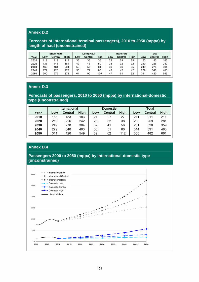
Annex D.2
Forecasts of international terminal passengers), 2010 to 2050 (mppa) by length of haul (unconstrained)
Low Central High Low Central High Low Central High Low Central High2010 119 119 119 36 36 36 29 29 29 183 183 1832020 135 148 161 42 46 50 33 32 32 210 226 2422030 160 184 204 50 58 64 39 36 35 249 278 3042040 179 226 273 56 72 88 43 42 42 279 340 4032050 200 279 372 64 90 125 47 51 52 311 420 549
YearTotalShort Haul Long Haul Transfers
Annex D.3
Forecasts of passengers, 2010 to 2050 (mppa) by international-domestic type (unconstrained)
Low Central High Low Central High Low Central High2010 183 183 183 27 27 27 211 211 2112020 210 226 242 28 32 38 238 259 2812030 249 278 304 32 41 56 281 320 3592040 279 340 403 36 51 80 314 391 4832050 311 420 549 39 62 112 350 482 661
International Domestic TotalYear
Annex D.4
Passengers 2000 to 2050 (mppa) by international-domestic type (unconstrained)
0
100
200
300
400
500
600
2000 2005 2010 2015 2020 2025 2030 2035 2040 2045 2050
International Low
International Central
International High
Domestic Low
Domestic Central
Domestic High
Historical data
151

Annex D.5
International passengers 2000 to 2050 (mppa) by journey purpose (unconstrained)
0
100
200
300
400
500
2000 2005 2010 2015 2020 2025 2030 2035 2040 2045 2050
mp
pa
Leisure Low
Leisure Central
Leisure High
Business Low
Business Central
Business High
Historic data
Annex D.6
Domestic passengers 2000 to 2050 (mppa) by journey purpose (unconstrained)
0
10
20
30
40
50
60
70
2000 2005 2010 2015 2020 2025 2030 2035 2040 2045 2050
mp
pa
Leisure Low
Leisure Central
Leisure High
Business Low
Business Central
Business High
Historic Business data
Historic Leisure data
152

Annex D.7
Business and leisure shares by region 2010 & 2030 (unconstrained)
Business Travel
52.5% 53.4% 53.1% 51.2%
10.3% 10.5% 9.7%9.0%
2.7% 2.8% 2.7%2.7%
7.6% 9.1% 9.0%8.7%
26.9% 24.1% 25.5% 28.5%
0%
10%
20%
30%
40%
50%
60%
70%
80%
90%
100%
2010 2030 Low 2030 Central 2030 High
Western Europe OECD (Non-European) Newly Industrialised Countries
Less Developed Countries Domestic (UK only)
Leisure Travel
65.9% 66.1% 66.0% 64.9%
11.2% 12.0% 11.2% 10.7%
3.0% 3.2% 3.1% 3.0%
11.2% 11.1% 10.9% 10.6%
8.6% 7.5% 8.8% 10.8%
0%
10%
20%
30%
40%
50%
60%
70%
80%
90%
100%
2010 2030 Low 2030 Central 2030 High
Western Europe OECD (Non-European) Newly Industrialised Countries
Less Developed Countries Domestic (UK only)
153

Annex D.8
Terminal passenger forecasts, central demand case, 2010-2050 (unconstrained)
Airport 2011 2020 2030 2040 2050
Heathrow 69.4 86.6 109.4 134.8 170.1Gatwick 33.6 38.3 39.8 45.3 51.9Manchester 18.8 24.5 30.3 37.0 45.7Stansted 18.0 23.4 26.3 32.2 37.9Luton 9.5 9.2 13.9 18.3 20.8Edinburgh 9.4 10.9 14.5 18.1 22.1Birmingham 8.6 11.4 13.9 17.2 22.7Glasgow 6.9 6.7 8.1 9.6 12.1Bristol 5.8 6.5 9.2 11.5 13.0Liverpool 5.2 4.7 5.3 6.1 6.8Newcastle 4.3 4.4 5.4 6.4 8.2East Midlands 4.2 3.3 4.2 5.2 7.1Belfast International 4.1 4.9 6.3 7.9 9.7Aberdeen 3.1 3.0 3.8 4.6 6.0London City 3.0 3.9 6.2 8.4 10.6Leeds/Bradford 2.9 3.6 5.7 7.4 9.2Belfast City 2.4 3.0 3.8 4.7 5.8Southampton 1.8 1.9 2.3 2.9 3.3Prestwick 1.3 1.5 1.3 1.3 1.3Cardiff 1.2 1.0 1.0 1.3 2.6Doncaster Sheffield 0.8 1.1 1.3 1.7 2.1Exeter 0.7 0.7 1.0 1.4 2.5Bournemouth 0.6 0.6 0.7 0.9 2.3Inverness 0.6 0.8 1.0 1.2 1.5Norwich 0.4 0.4 0.7 0.8 1.0Humberside 0.3 0.6 1.0 1.1 1.4Blackpool 0.2 0.1 0.4 0.5 0.6Newquay 0.2 0.5 0.5 0.6 0.8Durham Tees Valley 0.2 0.2 0.1 0.1 0.2Coventry 0.0 0.0 0.0 0.0 0.0Southend 0.0 1.0 2.2 2.3 2.5
1. 2011 f igures are CAA act uals.
2. Cen t ral d em and case
3. Modelled results are a notional scenario with no capacity constraints at any airport.
4. Airports sorted by 2011 throughput.
mppa
154

Annex D.9
Modelled international destinations served at selected UK airports 2011, 2030 & 2050 (unconstrained)
2011 2030 2050Heathrow 138 162 193Gatwick 75 85 106Stansted 55 66 80Luton 26 30 40London City 14 16 25Southend 0 4 1London** 178 208 246
Manchester 41 64 84Birmingham 22 32 52Glasgow 6 7 10Edinburgh 11 22 31Newcastle 6 10 14Belfast International 2 9 15Bristol 13 22 36Liverpool 15 18 22East Midlands 7 9 15Other modelled airports 19 39 55
Total** 178 209 251
**Total different destinations available, not sum of individual airport destinations
All types of carrier
* 2011 is modelled. Modelled numbers will vary slightly from observed patterns because they represent a full calendar observed data will include seasonal services and new start-ups or routes withdrawn during the course of the year.
155

Annex E Passenger forecasts (constrained)
E.1 This annex includes specific airport forecasts. This is for both continuity with previous publications and transparency of the forecasting methodology. At the airport level DfT forecasts may differ from local airport forecasts. The latter may be produced for different purposes and may be informed by specific commercial and local information.
E.2 It should be noted that while the DfT aims to accurately reflect existing planning restrictions on the expansion of airports, the forecasts should not in themselves be considered a cap on the development of individual airports. In some circumstances the airport specific forecasts could be used, in conjunction with additional relevant information, to inform local planning decisions.
E.3 While the range of demand scenarios adopted represents a range of outcomes at the national level, there may be additional factors that need to be considered when considering the degree of associated with particular airports.
E.4 The model is tasked with finding an equilibrium balance between demand and available capacity for all airports in the system. At times, particularly later in the period, this means that some limited variations around input passenger capacity are permitted to allow the modelling to converge at an equilibrium solution, resulting in some forecasts being marginally over input capacity.
E.5 Unrounded forecasts are presented. This is primarily to give transparency to modelling outputs. The use of unrounded figures does not reflect the underlying level of certainty around individual results.
156

Annex E.1
Forecasts of passengers by purpose and world region, 2010-2050 (constrained)
2020 2030 2040 2050Low Central High Low Central High Low Central High Low Central High
UK BusinessShort Haul 13.4 16.0 18.4 20.7 18.6 23.5 27.9 21.1 28.5 36.4 23.4 33.3
OECD 1.6 1.8 2.0 2.3 2.0 2.7 3.3 2.3 3.3 4.6 2.6 4.1NIC 0.6 0.7 0.9 1.0 0.9 1.2 1.5 1.0 1.3 1.8 1.2 1.6
LDC 1.6 2.6 3.1 3.5 3.0 4.0 4.9 3.4 4.9 6.7 3.8 6.0
All Long Haul 3.8 5.1 6.1 6.9 5.9 7.8 9.7 6.7 9.5 13.1 7.6 11.7All UK Business 17.2 21.2 24.5 27.6 24.5 31.3 37.6 27.8 38.0 49.5 31.0 45.0UK LeisureScheduled Short Haul 58.4 67.9 74.2 80.4 80.5 91.9 98.9 89.7 109.9 127.5 98.8 131.1
OECD 7.4 8.5 9.4 10.2 9.9 11.6 12.8 11.3 14.8 17.8 12.8 18.6
NIC 2.7 3.2 3.7 4.1 3.9 4.7 5.0 4.5 5.5 6.5 5.0 7.0LDC 9.5 10.8 11.8 12.8 12.7 14.8 16.1 14.4 18.6 21.9 16.2 23.5
All Scheduled Long Haul 19.6 22.6 25.0 27.0 26.6 31.2 33.9 30.2 38.8 46.2 34.0 49.1Short Haul Charter 16.0 15.2 16.7 18.2 18.0 20.7 22.4 20.0 25.3 29.6 22.2 31.1
Long Haul Charter 3.3 2.5 2.8 3.0 2.9 3.4 3.8 3.2 4.2 5.1 3.5 5.0
All Charter 19.3 17.6 19.5 21.3 20.9 24.1 26.3 23.2 29.5 34.7 25.8 36.1All Short Haul 74.4 83.1 90.9 98.6 98.5 112.6 121.3 109.6 135.2 157.1 121.0 162.1All Long Haul 22.9 25.0 27.7 30.1 29.5 34.6 37.7 33.4 43.1 51.3 37.5 54.2All UK Leisure 97.3 108.1 118.6 128.7 127.9 147.2 159.0 143.0 178.3 208.4 158.5 216.3Foreign BusinessShort Haul 9.9 10.6 11.9 13.1 12.0 14.5 16.9 13.2 17.2 21.4 14.4 20.1
OECD 1.7 1.8 2.0 2.2 2.0 2.4 2.9 2.2 2.9 3.7 2.4 3.4
NIC 0.3 0.4 0.4 0.5 0.4 0.5 0.6 0.5 0.6 0.8 0.5 0.7
LDC 1.2 1.3 1.4 1.6 1.4 1.7 2.1 1.6 2.0 2.6 1.7 2.4
All Long Haul 3.3 3.4 3.9 4.3 3.8 4.7 5.6 4.2 5.5 7.1 4.6 6.4All Foreign Business 13.3 14.0 15.8 17.4 15.7 19.2 22.5 17.4 22.7 28.5 19.0 26.5Foreign LeisureShort Haul 24.8 28.0 29.2 30.7 32.5 34.5 36.3 35.6 40.2 46.6 39.0 47.5
OECD 5.6 6.2 6.2 6.3 7.0 7.0 7.2 7.7 8.0 9.3 8.5 9.4
NIC 1.0 1.1 1.2 1.2 1.3 1.3 1.4 1.5 1.5 1.8 1.6 1.7LDC 3.2 3.6 3.6 3.6 4.1 4.0 4.1 4.5 4.7 5.5 5.0 5.5
All Long Haul 9.7 10.9 11.0 11.1 12.4 12.4 12.7 13.7 14.2 16.6 15.1 16.6All Foreign Leisure 34.5 38.9 40.2 41.7 44.9 46.9 48.9 49.3 54.4 63.2 54.1 64.1
International to International 21.1 25.5 23.7 22.7 31.0 27.0 24.0 33.4 28.6 25.7 37.2 36.2Transfer
Total UK International 114.5 129.3 143.1 156.3 152.4 178.5 196.6 170.8 216.3 257.9 189.5 261.3Total Foreign International 68.9 78.5 79.7 81.9 91.6 93.1 95.4 100.1 105.7 117.4 110.3 126.8Total International 183.4 207.7 222.9 238.2 244.0 271.6 292.0 270.9 322.0 375.3 299.8 388.0
Business 12.6 13.1 15.1 18.0 14.8 19.3 25.9 16.6 23.6 36.6 18.3 28.7Leisure 12.0 12.4 14.3 17.1 14.0 18.1 24.2 15.7 21.8 32.9 17.1 25.7Miscellaneous 2.5 2.5 2.9 3.4 2.8 3.6 4.6 3.2 4.3 6.2 3.4 5.0Total Domestic 27.2 28.1 32.4 38.4 31.7 41.0 54.7 35.4 49.8 75.6 38.8 59.4
GRAND TOTAL 210.5 235.8 255.2 276.6 275.8 312.6 346.7 306.4 371.7 450.9 338.6 447.5National Air Passenger Allocation Model failed to reach 2050.
1. International figures are terminal passengers and count domestic interlining passengers changing at hub airports.2. Scheduled figures include both "full service" and low cost airlines.3. Domestic passengers exclude those using domestic flights to connect to international flights at a hub airport.4. Miscellaneous includes passengers at minor airports not surveyed in the source data and other non-surveyed passengers such as
domestic charters, oil rig traffic etc., most, but not all, will be domestic.5. 2010 is modelled.
INTERNATIONAL
DOMESTIC (Internal "end to end")
(mppa) 2010
157

Annex E.2
Terminal passenger forecasts, central demand case, 2011-2050 (constrained)
Airport 2011 2020 2030 2040 2050
Heathrow 69.4 75.5 81.8 86.9 92.9Gatwick 33.6 37.3 40.6 42.6 44.2Manchester 18.8 22.1 28.1 39.0 55.2Stansted 18.0 25.4 35.7 36.0 35.4Luton 9.5 13.8 18.5 18.6 17.7Edinburgh 9.4 10.5 13.2 16.8 20.5Birmingham 8.6 11.8 16.7 28.2 38.3Glasgow 6.9 6.9 8.7 9.7 12.2Bristol 5.8 6.8 9.7 12.3 12.3Liverpool 5.2 5.3 6.7 8.2 15.4Newcastle 4.3 4.2 5.1 5.8 8.9East Midlands 4.2 3.6 4.4 9.0 14.1Belfast International 4.1 4.9 6.5 8.2 10.3Aberdeen 3.1 2.9 3.7 4.5 5.6London City 3.0 4.9 6.2 6.4 7.1Leeds/Bradford 2.9 4.4 6.4 8.3 8.4Belfast City 2.4 3.0 3.7 4.7 5.8Southampton 1.8 2.3 4.0 7.0 6.7Prestwick 1.3 1.8 2.0 2.2 2.6Cardiff 1.2 0.9 1.1 1.7 7.8Doncaster Sheffield 0.8 0.9 1.3 2.3 6.5Exeter 0.7 0.7 1.1 1.7 3.0Bournemouth 0.6 0.7 1.4 4.8 4.4Inverness 0.6 0.8 1.0 1.2 1.4Norwich 0.4 0.4 0.6 1.5 3.6Humberside 0.3 0.7 0.9 1.0 3.0Blackpool 0.2 0.3 0.4 0.4 0.3Newquay 0.2 0.5 0.5 0.5 1.2Durham Tees Valley 0.2 0.2 0.1 0.1 0.4Coventry 0.0 0.0 0.0 0.0 0.0Southend 0.0 1.5 2.5 2.3 2.3
1. 2011 figures are CAA actuals.
2. Central demand case.
3. Modelled results s02 scenario (max use of existing runways).
4. Input terminal capacities may be marginally exceeded to allow the model to converge to an equilibrium s
5. Airports sorted by 2011 throughput.
mppa
158

Annex E.3
Terminal passengers, forecast range, 2030 & 2050 (constrained)
2030 2050 2030 2050 2030 2050Heathrow 80.3 89.1 81.8 92.9 81.6Gatwick 38.9 41.1 40.6 44.2 41.1Manchester 24.2 33.5 28.1 55.2 32.3Stansted 30.5 35.4 35.7 35.4 35.3Luton 15.2 18.5 18.5 17.7 18.5Edinburgh 11.1 14.5 13.2 20.5 15.9Birmingham 11.3 19.4 16.7 38.3 25.3Glasgow 7.3 8.6 8.7 12.2 10.2Bristol 7.7 10.7 9.7 12.3 12.4Liverpool 5.1 6.7 6.7 15.4 7.7Newcastle 4.4 5.0 5.1 8.9 5.8East Midlands 3.7 5.8 4.4 14.1 6.2Belfast International 5.2 6.7 6.5 10.3 8.1Aberdeen 3.0 3.6 3.7 5.6 4.7London City 6.8 6.8 6.2 7.1 6.7Leeds/Bradford 6.4 8.0 6.4 8.4 7.1Belfast City 3.0 3.7 3.7 5.8 4.9Southampton 2.2 7.4 4.0 6.7 4.6Prestwick 1.7 1.5 2.0 2.6 2.3Cardiff 0.9 1.3 1.1 7.8 1.2Doncaster Sheffield 0.8 0.9 1.3 6.5 1.6Exeter 1.0 1.7 1.1 3.0 1.2Bournemouth 0.7 2.9 1.4 4.4 5.0Inverness 0.8 1.0 1.0 1.4 1.3Norwich 0.4 0.8 0.6 3.6 1.1Humberside 0.7 0.9 0.9 3.0 1.2Blackpool 0.3 0.3 0.4 0.3 0.4Newquay 0.4 0.3 0.5 1.2 0.5Durham Tees Valley 0.0 0.1 0.1 0.4 0.1Coventry 0.0 0.0 0.0 0.0 0.0Southend 1.8 2.5 2.5 2.3 2.3
National Air Passenger Allocation Model failed to reach 2050.
1. Range is und er ly ing d em and scenar ios, no t runw ay const rain t op t ions.
2. Mod elled result s s02 scenar io (m ax use o f exist ing runw ays).
3. High grow t h m od el runs d id no t reach 2050.
4. Input terminal capacities may be marginally exceeded to allow the model to converge to an equilibrium solution.
5. Airports sorted by 2011 throughput.
Airport
mppa
Low Central High
159

Annex E.4
UK runway capacity used, low - high range, max use, 2011-2050 (constrained)
Low 2011 2020 2030 2040 2050
Heathrow 99% 100% 100% 100% 100%Gatwick 90% 100% 100% 100% 100%Stansted 58% 58% 81% 100% 100%Luton 59% 48% 68% 100% 100%London City 56% 59% 100% 100% 100%Southend 28% 42% 42% 57%London 81% 81% 92% 97% 97%Manchester 49% 52% 49% 44% 52%Birmingham 45% 46% 56% 71% 99%Bristol 35% 33% 27% 36% 40%East Midlands 22% 17% 18% 20% 24%Southampton 27% 28% 34% 53% 100%Other modelled 22% 22% 25% 25% 29%National 39% 40% 44% 45% 50%
Central 2011 2020 2030 2040 2050
Heathrow 99% 100% 100% 100% 100%Gatwick 90% 100% 100% 100% 100%Stansted 58% 69% 100% 100% 100%Luton 59% 60% 100% 100% 100%London City 56% 87% 100% 100% 100%Southend 42% 100% 100% 100%London 81% 86% 100% 100% 100%Manchester 49% 57% 55% 58% 100%Birmingham 45% 56% 79% 100% 100%Bristol 35% 38% 37% 100% 100%East Midlands 22% 17% 20% 43% 100%Southampton 27% 36% 52% 100% 100%Other modelled 22% 24% 28% 33% 43%National 39% 43% 50% 54% 63%
High 2011 2020 2030 2040 2050
Heathrow 99% 100% 100% 100%Gatwick 90% 100% 100% 100%Stansted 58% 77% 100% 100%Luton 59% 70% 100% 100%London City 56% 100% 100% 100%Southend 54% 100% 100%London 81% 92% 100% 100%Manchester 49% 61% 64% 100%Birmingham 45% 64% 100% 100%Bristol 35% 49% 100% 100%East Midlands 22% 18% 26% 100%Southampton 27% 38% 58% 100%Other modelled 22% 26% 35% 45%National 39% 47% 56% 64%100% = runway or terminal capacity exceeded, other %s refer to runway usage.
Mainland UK airports only.National Air Passenger Allocation Model failed to reach 2050.
160

Annex E.5
Terminal passengers by world destination, excluding transfers, max use, 2010-2050 (constrained)
2010 2020 2030 2040 2050Domestic 27 32 41 50 59Europe 119 148 183 220 263Rest of Africa 6 6 7 9 11United States and Canada 14 17 21 26 33Caribbean & South America 3 4 5 6 8Middle East 5 8 10 13 16Indian Sub-continent 3 3 4 6 7Far East 4 6 7 9 11Australasia 2 2 2 3 3Total (exc. Transfers) 182 226 281 342 411
1. Modelled results from the s02 max use of existing runways scenario
3. Passengers beginning or ending their journeys in the UK, i.e. excluding international-international transfers4. 2010 is modelled.
mppa
2. Europe SH includes African Mediterranean holiday destinations, excl Egypt and Israel
Annex E.6
Transfer passengers, max use, 2010-2050 (constrained)
2010 2020 2030 2040 2050Domestic-international transfers Heathrow 5.5 2.5 0.5 0.3 0.2
Gatwick 1.5 2.0 2.2 0.7 0.1Other UK 0.5 0.9 1.5 0.4 0.1
Total 7.4 5.3 4.1 1.4 0.4UK transfers at overseas hubs European Hub 2.2 1.7 1.3 1.5 2.2
Middle East 1.7 1.9 2.0 2.0 3.2Total 4.0 3.5 3.4 3.5 5.4
International-international transfers Heathrow 18.0 21.0 23.3 23.6 26.9Gatwick 1.7 2.1 2.6 2.5 1.1Other UK 1.4 0.6 1.1 2.5 8.2
Total 21.1 23.7 27.0 28.6 36.2Grand total 32.5 32.6 34.5 33.5 42.0
Notes1. Modelled results from the s02 scenario (max use of existing runways)2. Domestic-international transfers at UK airports count each passenger *2 at the UK hub, but not at the UK originating airport3. Domestic international transfers at overseas airport count each passenger *1 at UK originating airport4. Proxy European airport hubs in model are Amsterdam, Paris CDG and Frankfurt5. Proxy Middle East hub is Dubai6. Transfers at other airports e.g. US or Far East hubs are not modelled7. International-international transfers have used UK hubs, but have ultimate origin or destination outside the UK8. 2010 figures are modelled, not actuals
mppaHub
161

162
Annex E.7
Terminal passengers by region of surface journey to airport origin, max use, 2010-2050 (constrained)
Surface to SE airports 2010 2020 2030 2040 2050
Northern Ireland 0 0 0 0 0Scotland 0 0 0 0 0North 2 2 2 1 1Midlands 6 9 10 7 5Wales 1 1 1 1 1South West 5 6 7 6 5
Regional total 14 19 20 15 12SE passengers 89 112 136 156 167Total surface passengers at SE airports 103 131 157 171 179Other airports
Northern Ireland 6 7 9 12 16Scotland 20 23 29 34 42North 28 34 43 54 66Midlands 13 15 19 29 39Wales 3 4 5 7 9South West 7 8 11 16 21
Regional total 77 90 117 153 193SE passengers 2 4 7 17 39Total surface passengers at other airports 78 95 124 171 231
Passengers with regional O-Ds
Northern Ireland 6 7 9 12 16Scotland 20 23 29 34 42North 30 35 45 55 66Midlands 19 24 30 36 44Wales 4 5 7 8 10South West 12 14 18 22 26South East 91 116 143 173 206
Total surface passengers 181 226 281 341 411I to I interliners at SE airports 21 24 27 27 28I to I interliners at regional airports 0 0 0 2 8Domestic interliners at SE airports 7 5 4 1 0Domestic interliners at regional airports 0 0 0 0 0Grand total 210 255 312 371 4471. SE Regional Airports: Heathrow, Gatwick, Stansted, Luton, London City, Southampton, Southend and Norwich.2. SE Passengers are from London, South East and Eastern Regions.
3. Domestic Interliners are counted as surface passengers to first airport and interliners (*2) at the hub.4. Passengers may not total exactly as a result of rounding to nearest million.
5. 2010 figures are modelled.6. All figures include only the 31 modelled UK airports.
max use, million passengers

Annex E.8
Terminal passengers by length of haul and journey purpose, 2010, modelled (constrained)
2010 Grandmppa Bus Lei Misc Total UKBus UKLei FoBus FoLei Total UKBus UKLei FoBus FoLei Total I to I from UK Total Total
Heathrow 1.2 1.0 0.1 2.2 4.7 6.5 3.8 4.8 19.7 3.1 10.1 2.7 5.7 21.6 18.0 5.5 23.5 67.1Gatwick 0.8 1.0 0.1 1.9 1.7 13.7 1.1 4.4 20.9 0.2 3.9 0.2 1.2 5.6 1.7 1.5 3.2 31.5Stansted 0.6 0.7 0.1 1.4 1.7 8.1 1.3 4.2 15.2 0.0 0.0 0.0 0.0 0.0 1.2 0.3 1.5 18.0Luton 0.7 0.3 0.1 1.0 0.8 5.1 0.6 2.2 8.6 0.0 0.0 0.0 0.0 0.1 0.0 0.0 0.0 9.7London City 0.4 0.2 0.2 0.8 0.4 0.6 0.3 0.6 1.9 0.0 0.0 0.0 0.0 0.1 0.0 0.0 0.0 2.8Southend 0.0 0.0 0.0 0.0 0.0 0.0 0.0 0.0 0.0 0.0 0.0 0.0 0.0 0.0 0.0 0.0 0.0 0.0London Total 3.7 3.1 0.5 7.3 9.2 34.0 7.1 16.1 66.4 3.3 14.1 3.0 7.0 27.3 21.0 7.2 28.2 129.2Manchester 0.5 0.4 0.1 1.0 0.9 8.3 0.8 1.4 11.4 0.3 3.8 0.2 0.8 4.9 0.1 0.2 0.3 17.7Birmingham 0.5 0.4 0.1 1.0 0.5 4.4 0.5 0.8 6.2 0.0 0.8 0.0 0.2 1.0 0.0 0.0 0.0 8.2Glasgow 1.6 0.6 0.2 2.4 0.2 1.9 0.1 0.4 2.5 0.1 0.7 0.0 0.3 1.2 0.0 0.0 0.0 6.0Edinburgh 1.8 1.7 0.1 3.7 0.6 2.7 0.3 1.2 4.7 0.0 0.3 0.0 0.2 0.5 0.0 0.0 0.0 9.0Bristol 0.3 0.5 0.0 0.8 0.2 3.9 0.1 0.7 4.9 0.0 0.1 0.0 0.0 0.1 0.0 0.0 0.0 5.8Newcastle 0.5 0.6 0.0 1.0 0.2 2.2 0.1 0.2 2.7 0.0 0.3 0.0 0.1 0.4 0.0 0.0 0.0 4.1Belfast International 0.8 1.3 0.0 2.0 0.1 1.4 0.0 0.1 1.7 0.0 0.0 0.0 0.0 0.1 0.0 0.0 0.0 3.8Liverpool 0.2 0.3 0.2 0.6 0.3 3.0 0.2 1.1 4.5 0.0 0.0 0.0 0.0 0.0 0.0 0.0 0.0 5.2East Midlands 0.3 0.2 0.0 0.5 0.2 3.2 0.1 0.4 3.8 0.0 0.1 0.0 0.0 0.1 0.0 0.0 0.0 4.3Other Airports in Model 2.6 3.0 1.2 6.8 0.8 7.2 0.6 1.4 10.0 0.0 0.3 0.0 0.1 0.5 0.0 0.0 0.0 17.3Regional Total 9.0 8.9 2.0 19.9 4.0 38.0 2.7 7.7 52.4 0.4 6.4 0.3 1.7 8.8 0.1 0.2 0.1 81.2National Total 12.6 12.0 2.5 27.2 13.1 72.0 9.8 23.8 118.7 3.7 20.5 3.2 8.7 36.1 21.1 7.4 28.5 210.51. Domestic total only includes "end to end" domestic travel and excludes transfers
2. Modelled results from the s02 scenario (max use of existing runways)
3. Long haul includes "medium haul" destinations to Midle East and North America.
4. UK to Channel Isles counted as short haul
5. I to I Hub transfers are not counted as part of the short haul / long haul categories
6. UK based transfers are not purpose split at the hub: purpose split totals will be lower than in Table E.1
7. 2010 results are modelled.
Short haul Long haul Hub transfersDomestic (Excl. intl transfers)
163

Annex E.9
Terminal passengers by length of haul and journey purpose, 2030, max use (constrained)
2030 Grandmppa Bus Lei Misc Total UKBus UKLei FoBus FoLei Total UKBus UKLei FoBus FoLei Total I to I from UK Total Total
Heathrow 0.4 0.4 0.1 0.8 7.3 7.2 4.9 4.7 24.1 5.8 16.0 3.7 7.6 33.1 23.3 0.5 23.8 81.8Gatwick 1.3 1.4 0.1 2.8 2.6 15.0 1.5 5.4 24.5 0.7 5.4 0.4 1.9 8.5 2.6 2.2 4.8 40.6Stansted 1.0 1.1 0.1 2.3 2.9 16.2 2.0 7.6 28.7 0.3 1.6 0.1 0.5 2.5 0.8 1.4 2.2 35.7Luton 1.8 1.4 0.1 3.3 1.7 9.6 0.9 3.0 15.2 0.0 0.0 0.0 0.0 0.0 0.1 0.0 0.1 18.5London City 1.0 0.3 0.2 1.4 1.2 1.8 0.7 1.1 4.8 0.0 0.0 0.0 0.0 0.0 0.0 0.0 0.0 6.2Southend 0.1 0.1 0.0 0.2 0.2 1.3 0.2 0.7 2.4 0.0 0.0 0.0 0.0 0.0 0.0 0.0 0.0 2.5London Total 5.5 4.6 0.6 10.8 15.9 51.1 10.2 22.5 99.6 6.9 23.0 4.2 10.0 44.1 26.8 4.0 30.8 185.3Manchester 0.7 0.6 0.2 1.5 1.7 14.2 1.1 2.2 19.3 0.6 5.2 0.3 1.1 7.1 0.2 0.1 0.3 28.1Birmingham 0.8 0.6 0.2 1.5 1.3 8.2 0.9 2.0 12.5 0.1 2.3 0.0 0.2 2.6 0.0 0.0 0.0 16.7Glasgow 2.6 1.3 0.3 4.2 0.2 2.3 0.1 0.3 2.9 0.1 1.0 0.0 0.4 1.5 0.0 0.0 0.0 8.7Edinburgh 2.7 2.3 0.2 5.1 1.2 4.2 0.4 2.0 7.8 0.1 0.1 0.0 0.1 0.3 0.0 0.0 0.0 13.2Bristol 0.5 0.7 0.0 1.1 0.3 6.3 0.2 0.9 7.6 0.0 0.9 0.0 0.0 0.9 0.0 0.0 0.0 9.7Newcastle 0.7 0.8 0.0 1.5 0.2 2.8 0.1 0.2 3.4 0.0 0.2 0.0 0.0 0.3 0.0 0.0 0.0 5.1Belfast International 1.4 2.3 0.0 3.7 0.2 2.2 0.1 0.2 2.7 0.0 0.1 0.0 0.0 0.2 0.0 0.0 0.0 6.5Liverpool 0.3 0.5 0.3 1.0 0.3 3.9 0.2 1.1 5.6 0.0 0.0 0.0 0.0 0.0 0.0 0.0 0.0 6.7East Midlands 0.4 0.2 0.0 0.6 0.1 3.4 0.0 0.2 3.7 0.0 0.1 0.0 0.0 0.1 0.0 0.0 0.0 4.4Other Airports in Model 3.8 4.3 1.8 9.9 1.8 12.4 1.0 2.6 17.8 0.0 0.3 0.0 0.1 0.4 0.0 0.0 0.0 28.1Regional Total 13.7 13.5 2.9 30.2 7.4 60.0 4.2 11.7 83.3 0.9 10.2 0.4 2.0 13.4 0.2 0.1 0.2 127.2National Total 19.3 18.1 3.6 41.0 23.3 111.1 14.4 34.2 182.9 7.7 33.3 4.6 12.0 57.6 27.0 4.1 31.1 312.61. Domestic total only includes "end to end" domestic travel and excludes transfers
2. Modelled results from the s02 scenario (max use of existing runways)
3. Long haul includes "medium haul" destinations to Midle East and North America.
4. UK to Channel Isles counted as short haul
5. I to I Hub transfers are not counted as part of the short haul / long haul categories
6. UK based transfers are not purpose split at the hub: purpose split totals will be lower than in Table E.1
7. Input terminal capacities may be marginally exceeded to allow the model to converge to an equilibrium solution.
Hub transfersDomestic (Excl. intl transfers) Short haul Long haul
164

165
Annex E.10
Terminal passengers by length of haul and journey purpose, 2050, max use (constrained)
2050 Grandmppa Bus Lei Misc Total UKBus UKLei FoBus FoLei Total UKBus UKLei FoBus FoLei Total I to I from UK Total Total
Heathrow 0.5 0.5 0.1 1.1 7.9 2.8 4.7 1.9 17.3 7.1 24.6 4.9 10.6 47.3 26.9 0.2 27.2 92.9Gatwick 1.0 1.3 0.1 2.5 3.3 20.2 1.9 6.3 31.7 0.9 5.8 0.5 1.7 8.9 1.1 0.1 1.2 44.2Stansted 1.8 1.4 0.1 3.3 3.6 16.5 2.8 9.2 32.0 0.0 0.0 0.0 0.0 0.0 0.0 0.0 0.1 35.4Luton 3.4 2.4 0.1 5.9 2.2 4.8 1.5 3.2 11.7 0.0 0.0 0.0 0.0 0.0 0.0 0.0 0.0 17.7London City 1.2 0.3 0.2 1.6 2.3 1.1 1.4 0.7 5.5 0.0 0.0 0.0 0.0 0.0 0.0 0.0 0.0 7.1Southend 0.1 0.2 0.0 0.3 0.3 0.9 0.2 0.7 2.1 0.0 0.0 0.0 0.0 0.0 0.0 0.0 0.0 2.3London Total 8.0 6.0 0.6 14.7 19.6 46.3 12.5 22.0 100.3 8.0 30.4 5.4 12.3 56.2 28.1 0.3 28.4 199.7Manchester 1.0 0.8 0.3 2.1 2.9 23.8 2.1 4.5 33.3 0.8 9.7 0.4 1.6 12.5 7.3 0.0 7.3 55.2Birmingham 1.0 0.6 0.2 1.8 1.3 15.1 0.9 3.7 21.0 2.6 10.0 0.4 1.7 14.7 0.8 0.0 0.8 38.3Glasgow 3.5 1.5 0.4 5.4 0.2 3.9 0.1 0.5 4.7 0.1 1.4 0.0 0.5 2.1 0.0 0.0 0.0 12.2Edinburgh 4.4 3.4 0.2 8.0 1.7 6.4 0.6 2.9 11.6 0.1 0.5 0.0 0.2 0.9 0.0 0.0 0.0 20.5Bristol 0.7 0.8 0.0 1.5 0.5 8.1 0.2 1.2 10.2 0.0 0.6 0.0 0.0 0.6 0.0 0.0 0.0 12.3Newcastle 1.0 1.1 0.0 2.1 0.3 5.1 0.2 0.4 6.0 0.0 0.9 0.0 0.0 0.9 0.0 0.0 0.0 8.9Belfast International 2.1 3.5 0.0 5.6 0.2 3.6 0.2 0.3 4.2 0.0 0.3 0.0 0.1 0.4 0.0 0.0 0.0 10.3Liverpool 0.4 0.8 0.4 1.6 0.6 10.3 0.4 2.4 13.8 0.0 0.0 0.0 0.0 0.0 0.0 0.0 0.0 15.4East Midlands 0.7 0.6 0.0 1.3 0.9 8.3 0.6 2.9 12.6 0.0 0.2 0.0 0.0 0.2 0.0 0.0 0.0 14.1Other Airports in Model 5.9 6.6 2.7 15.2 5.0 31.2 2.2 6.7 45.2 0.0 0.1 0.0 0.1 0.3 0.0 0.0 0.0 60.7Regional Total 20.7 19.7 4.4 44.7 13.7 115.9 7.5 25.5 162.6 3.6 23.7 0.9 4.2 32.4 8.1 0.0 8.1 247.8National Total 28.7 25.7 5.0 59.4 33.3 162.1 20.0 47.5 262.9 11.7 54.1 6.3 16.5 88.6 36.2 0.4 36.6 447.51. Domestic total only includes "end to end" domestic travel and excludes transfers
2. Modelled results from the s02 scenario (max use of existing runways)
3. Long haul includes "medium haul" destinations to Midle East and North America.
4. UK to Channel Isles counted as short haul
5. I to I Hub transfers are not counted as part of the short haul / long haul categories
6. UK based transfers are not purpose split at the hub: purpose split totals will be lower than in Table E.1
7. Input terminal capacities may be marginally exceeded to allow the model to converge to an equilibrium solution.
Domestic (Excl. intl transfers) Short haul Long haul Hub transfers

Annex E.11
Destinations served split by airline type, 2010-2050 (constrained)
2011 2020 2030 2040 2050 2011 2020 2030 2040 2050 2011 2020 2030 2040 2050
Heathrow 174 173 168 170 155 0 0 0 0 0 0 0 0 0 0
Gatwick 133 148 140 124 94 99 103 73 70 54 109 63 69 69 62
Manchester 80 91 117 140 163 65 54 58 59 54 100 75 84 100 121
Birmingham 52 70 82 113 88 27 37 43 46 48 65 40 43 41 39
Luton 50 56 64 52 37 51 21 19 11 12 19 24 28 28 0
Stansted 32 37 45 40 15 114 102 108 110 109 32 21 19 1 1
Southampton 29 33 48 45 27 0 0 0 0 0 2 1 0 1 0
London City 26 38 44 28 18 0 0 0 0 0 0 0 0 0 0
Edinburgh 16 18 28 36 39 60 82 89 98 90 10 7 5 8 10
Glasgow 12 12 12 13 17 8 3 3 2 5 39 40 47 48 53
Belfast International 12 14 17 19 26 18 22 24 26 26 10 10 13 16 22
Exeter 12 14 19 29 29 0 0 1 2 22 9 9 11 12 1
Newcastle 10 8 12 17 15 23 23 23 24 29 43 40 41 43 59
Bristol 9 9 14 14 41 60 58 69 74 36 38 32 31 31 29
Aberdeen 9 12 13 15 16 1 1 3 4 8 2 1 1 1 5
Doncaster Sheffield 9 4 2 11 15 6 0 0 0 0 21 20 19 20 21
Liverpool 4 3 10 12 22 65 45 39 40 63 1 0 0 1 2
Leeds/Bradford 3 2 1 2 1 47 63 65 66 61 17 3 1 0 0
Cardiff 3 3 4 5 7 10 5 4 3 47 18 15 13 18 18
Prestwick 2 3 4 8 8 22 17 17 16 17 0 0 0 0 0
Belfast City 2 3 3 4 8 0 0 0 0 0 0 0 0 1 1
East Midlands 1 1 1 31 40 49 24 22 21 59 38 23 25 29 29
Durham Tees Valley 1 1 0 0 5 0 0 0 0 0 3 1 0 0 0
Bournemouth 1 2 6 30 28 12 10 11 13 8 7 5 2 2 0
Inverness 1 2 2 2 2 0 0 0 0 0 0 0 0 0 0
Norwich 1 1 3 12 31 0 0 0 0 1 5 0 0 6 1
Humberside 1 10 13 13 31 0 0 0 0 0 2 1 1 0 0
Newquay 1 2 2 2 8 0 0 0 0 1 0 0 0 0 0
Blackpool 1 3 3 3 1 3 0 0 0 0 0 0 0 0 0
Coventry 0 0 0 0 0 0 0 0 0 0 0 0 0 0 0
Southend 0 5 5 5 7 0 11 15 11 6 0 0 0 0 0
Total 687 778 882 995 994 740 681 686 696 756 590 431 453 476 474
1. Destinations counted if more than 5,000 passengers allocated to the destination.
2. 2011 are modelled and counted on the same basis and may differ from CAA actuals based on service frequency.
3. Airports sorted by 'full service' modelled scheduled routes, 2011.
Scheduled LCC Charter
Annex E.12
Billion revenue passenger-kms (constrained)
Low Central High2010 581 581 5812015 627 644 6652020 683 729 7772025 753 816 8702030 819 900 9712035 862 979 1,1032040 916 1,086 1,2792045 973 1,2212050 1,029 1,341
National Air Passenger Allocation Model failed to reach 2050.
3. RPK counts both arriving and departing passengers.
2. Revenue Passenger-kms (RPK) counted only for passengers at the 31 UK airports in the model.
1. Modelled results from the core "s02" max use of existing runways scenario
166

Annex F: ATM forecasts (constrained)
F.1 For transparency, the numbers presented in this annex are direct unrounded model outputs. The model is tasked with finding an equilibrium balance between demand and available capacity for all airports in the system. At times, particularly later in the period, this means that some limited variations around input ATM capacity are permitted to occur to allow the modelling to converge at an equilibrium solution, resulting in some forecasts marginally over input capacity. In this annex, unlike Annex E, a capped to capacity figure will be shown where there has been a breach, but this will be shown on the table by bold italic format and the direct model output will also be given in the supplementary tables published alongside this report.
F.2 Unrounded forecasts are presented in this annex. This is primarily to give transparency to modelling outputs. The use of unrounded figures does not reflect the underlying level of certainty around individual results.
F.3 The direct model output is used in the CO2 calculations reported in Annex G.
167

Annex F.1
ATMs by domestic/international, scheduled/charter, passenger/freight, 2010-2050, central forecast, max use (constrained)
ATM 000s
International Scheduled
International Charter Domestic Freight Total
2010 1,294 101 550 51 1,9962015 1,370 91 561 55 2,0772020 1,514 104 602 55 2,2742025 1,678 116 661 56 2,5112030 1,844 127 695 59 2,7242035 2,024 139 742 59 2,9642040 2,216 150 788 61 3,2152045 2,485 164 816 59 3,5252050 2,676 174 858 60 3,768
1. ATMs are counted at the 31 UK airports included in the DfT model.
2. All figures are modelled, including 2010.
3. Modelled results from s02 scenario (maximum use of existing runways)
4. ATMs exclude general aviation, air taxis, positional, diplomatic, military and other miscellaneous flights.
Annex F.2
ATMs by South East airport 2010-2050, central forecast, max use (constrained)
ATM 000s Heathrow Gatwick Stansted LutonLondon
CityTotal
LondonLondon Share
Other Airports Total
2010 480 234 155 79 66 1,014 51% 975 1,9892015 480 265 165 76 75 1,060 51% 1,004 2,0642020 480 269 179 97 104 1,129 50% 1,113 2,2422025 480 280 207 118 120 1,205 49% 1,255 2,4602030 480 280 253 134 120 1,266 47% 1,413 2,6792035 480 280 252 134 120 1,266 43% 1,646 2,9122040 480 280 259 135 120 1,274 40% 1,872 3,1462045 480 277 246 131 120 1,254 36% 2,207 3,4612050 478 280 253 134 120 1,265 35% 2,391 3,656
1. Other ATMs are counted at the remaining 26 UK airports included in the DfT model.2. All figures are modelled, including 20103. ATMs unrounded.4. Model results for the Central Demand Case, s02 scenario (max use of existing runways)5. ATMs exclude general aviation, air taxis, positional, diplomatic, military and other miscellaneous flights.6. Individual airport totals capped strictly to capacity, modelling constraint tolerances removed, model output totals may differ from F.17. Bold italic numbers are the individual airport totals capped to capacity. Uncapped versions are in the supplementary tables
168

Annex F.3
ATM forecasts at UK airports, 2010-2050 central forecast, max use (constrained)
Airport 2011 2020 2030 2040 2050
Heathrow 476.9 480.0 480.0 480.0 478.2Gatwick 244.8 268.6 280.0 280.0 280.0Manchester 158.2 184.2 221.2 291.9 433.7Stansted 138.8 179.3 252.5 259.0 252.8Edinburgh 108.7 117.0 140.8 160.2 173.8Aberdeen 99.5 100.0 123.0 139.2 150.0Birmingham 84.7 114.7 161.9 206.0 194.0Luton 76.2 96.7 133.7 134.9 133.7Glasgow 72.4 65.6 78.8 88.0 100.8London City 67.4 104.1 120.0 120.0 120.0East Midlands 58.4 45.8 51.7 114.2 193.8Bristol 52.8 57.5 84.0 105.0 122.2Liverpool 46.2 41.0 55.0 65.2 121.6Newcastle 45.1 45.2 54.4 59.8 78.8Southampton 41.3 54.2 78.1 126.1 121.4Belfast City 41.2 45.7 55.5 68.8 82.7Belfast International 38.3 48.6 61.8 77.9 97.0Leeds/Bradford 33.4 42.6 58.3 76.3 78.3Norwich 19.5 20.6 28.0 45.1 79.3Cardiff 16.2 14.4 20.3 27.4 75.3Inverness 15.1 16.3 22.1 29.4 30.0Humberside 13.3 25.6 30.4 33.4 48.8Exeter 12.7 13.2 17.7 26.4 35.7Blackpool 10.2 9.8 10.7 10.9 9.5Prestwick 10.0 12.3 14.2 15.9 18.6Newquay 6.9 12.6 15.2 16.8 32.6Bournemouth 6.3 8.6 18.9 72.9 78.2Durham Tees Valley 6.3 4.7 2.5 2.5 9.1Doncaster Sheffield 6.2 6.0 7.7 12.2 59.7Coventry 0.7 0.2 0.2 0.2 0.2Southend 19.2 27.8 27.2 28.6
1. 2011 figures are CAA actuals, but only include modelled commercial scheduled and charter services
2. Central demand case
3. Modelled results s02 scenario (max use of existing runways).
4. Bold italic numbers are the individual airport totals capped to capacity.Uncapped versions are in the
supplementary tables.
5. Airports sorted by 2011 ATM throughput.
thousands
169

Annex F.4
ATM forecasts at UK airports, 2030 & 2050, low-high range, max use (constrained)
2030 2050 2030 2050 2030 2050Heathrow 480 480 480 478 480Gatwick 280 280 280 280 279Manchester 197 259 221 434 257Stansted 211 247 253 253 257Edinburgh 130 169 141 174 162Aberdeen 115 143 123 150 135Birmingham 116 205 162 194 206Luton 109 138 134 134 135Glasgow 71 81 79 101 89London City 120 119 120 120 120East Midlands 47 62 52 194 69Bristol 61 90 84 122 109Liverpool 38 52 55 122 62Newcastle 48 54 54 79 61Southampton 51 127 78 121 87Belfast City 47 60 56 83 68Belfast International 51 65 62 97 75Leeds/Bradford 56 69 58 78 68Norwich 25 39 28 79 35Cardiff 18 23 20 75 21Inverness 17 26 22 30 29Humberside 28 35 30 49 35Exeter 16 23 18 36 22Blackpool 10 10 11 10 11Prestwick 13 12 14 19 17Newquay 12 15 15 33 17Bournemouth 9 45 19 78 80Durham Tees Valley 2 3 3 9 3Doncaster Sheffield 5 6 8 60 9Coventry 0 0 0 0 0Southend 22 30 28 29 26
National Air Passenger Allocation Model failed to reach 2050.
1. Range is underlying demand scenarios, not runway constraint options.
2. Modelled results s02 scenario (max use of existing runways).
3. Bold italic numbers are the individual airport totals capped to capacity.Uncapped versions are in the supplementary
tables.4. Airports sorted by 2011 ATM throughput.
Low Central HighAirport
170

Annex G: CO2 emission forecasts (constrained)
171

Annex G.1
CO2 emissions by UK airport, 2030/2050, low-central-high range, max use, (constrained)
2030 2050Low Central High Low Central High
Heathrow 21.2 21.4 22.1 15.6 18.2 20.0Gatwick 4.3 4.7 4.8 3.5 4.3 5.0Stansted 2.9 3.5 3.0 2.4 1.9 2.1Manchester 2.6 3.2 3.8 3.0 5.3 5.4Birmingham 1.0 1.7 3.6 1.4 4.6 4.6Luton 1.1 1.3 1.2 1.3 0.9 0.9Edinburgh 0.6 0.7 0.9 0.7 1.0 1.0Bristol 0.5 0.7 1.0 0.7 1.0 0.9Glasgow 0.6 0.7 0.8 0.5 0.8 1.1London City 0.5 0.5 0.5 0.3 0.5 0.5Liverpool 0.3 0.4 0.4 0.3 0.9 0.9Leeds/Bradford 0.5 0.4 0.4 0.6 0.4 0.4Belfast International 0.3 0.3 0.4 0.3 0.5 0.6East Midlands 0.3 0.3 0.5 0.4 1.1 1.1Newcastle 0.3 0.3 0.4 0.3 0.5 1.0Southampton 0.2 0.3 0.3 0.5 0.4 0.4Aberdeen 0.2 0.2 0.3 0.1 0.2 0.3Prestwick 0.1 0.2 0.2 0.1 0.2 0.3Belfast City 0.1 0.1 0.2 0.1 0.2 0.3Humberside 0.1 0.1 0.2 0.1 0.3 0.4Southend 0.1 0.1 0.1 0.1 0.1 0.1Bournemouth 0.0 0.1 0.5 0.3 0.4 0.4Doncaster Sheffield 0.1 0.1 0.1 0.1 0.5 0.5Cardiff 0.1 0.1 0.1 0.1 0.4 0.4Exeter 0.1 0.1 0.1 0.1 0.2 0.3Inverness 0.0 0.1 0.1 0.0 0.0 0.1Newquay 0.0 0.0 0.0 0.0 0.1 0.2Norwich 0.0 0.0 0.1 0.0 0.3 0.2Blackpool 0.0 0.0 0.0 0.0 0.0 0.3Durham Tees Valley 0.0 0.0 0.0 0.0 0.1 0.2Ground (APU) 0.5 0.5 0.6 0.6 0.7 0.8Freight 1.2 1.2 1.2 0.9 0.9 1.0Residual 0.1 0.1 0.1 0.1 0.1 0.1Total 39.7 43.5 48.2 34.7 47.0 52.1
Notes
1. Low CO2 assumes low demand scenario
2. High CO2 assumes high demand scenario
3. All cases are for the option 's02': 'Max use' scenario,
4. Airports sorted on 2030 central CO2 emissions.
5. CO2 emissions from UK departures only.
6. APU, freight and residual add-on not allocated to airports.
million tonnes CO2
172
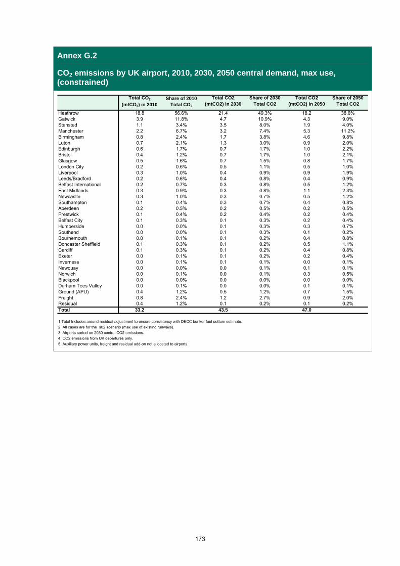
173
Annex G.2
CO2 emissions by UK airport, 2010, 2030, 2050 central demand, max use, (constrained)
Total CO2
(mtCO2) in 2010Share of 2010
Total CO2
Total CO2 (mtCO2) in 2030
Share of 2030 Total CO2
Total CO2 (mtCO2) in 2050
Share of 2050 Total CO2
Heathrow 18.8 56.6% 21.4 49.3% 18.2 38.6%Gatwick 3.9 11.8% 4.7 10.9% 4.3 9.0%Stansted 1.1 3.4% 3.5 8.0% 1.9 4.0%Manchester 2.2 6.7% 3.2 7.4% 5.3 11.2%Birmingham 0.8 2.4% 1.7 3.8% 4.6 9.8%Luton 0.7 2.1% 1.3 3.0% 0.9 2.0%Edinburgh 0.6 1.7% 0.7 1.7% 1.0 2.2%Bristol 0.4 1.2% 0.7 1.7% 1.0 2.1%Glasgow 0.5 1.6% 0.7 1.5% 0.8 1.7%London City 0.2 0.6% 0.5 1.1% 0.5 1.0%Liverpool 0.3 1.0% 0.4 0.9% 0.9 1.9%Leeds/Bradford 0.2 0.6% 0.4 0.8% 0.4 0.9%Belfast International 0.2 0.7% 0.3 0.8% 0.5 1.2%East Midlands 0.3 0.9% 0.3 0.8% 1.1 2.3%Newcastle 0.3 1.0% 0.3 0.7% 0.5 1.2%Southampton 0.1 0.4% 0.3 0.7% 0.4 0.8%Aberdeen 0.2 0.5% 0.2 0.5% 0.2 0.5%Prestwick 0.1 0.4% 0.2 0.4% 0.2 0.4%Belfast City 0.1 0.3% 0.1 0.3% 0.2 0.4%Humberside 0.0 0.0% 0.1 0.3% 0.3 0.7%Southend 0.0 0.0% 0.1 0.3% 0.1 0.2%Bournemouth 0.0 0.1% 0.1 0.2% 0.4 0.8%Doncaster Sheffield 0.1 0.3% 0.1 0.2% 0.5 1.1%Cardiff 0.1 0.3% 0.1 0.2% 0.4 0.8%Exeter 0.0 0.1% 0.1 0.2% 0.2 0.4%Inverness 0.0 0.1% 0.1 0.1% 0.0 0.1%Newquay 0.0 0.0% 0.0 0.1% 0.1 0.1%Norwich 0.0 0.1% 0.0 0.1% 0.3 0.5%Blackpool 0.0 0.0% 0.0 0.0% 0.0 0.0%Durham Tees Valley 0.0 0.1% 0.0 0.0% 0.1 0.1%Ground (APU) 0.4 1.2% 0.5 1.2% 0.7 1.5%Freight 0.8 2.4% 1.2 2.7% 0.9 2.0%Residual 0.4 1.2% 0.1 0.2% 0.1 0.2%Total 33.2 43.5 47.0
1.Total Includes around residual adjustment to ensure consistency with DECC bunker fuel outturn estimate.
2. All cases are for the s02 scenario (max use of existing runways).
3. Airports sorted on 2030 central CO2 emissions.
4. CO2 emissions from UK departures only.
5. Auxiliary power units, freight and residual add-on not allocated to airports.

Annex G.3
ATMs (short vs long haul), available seat-kms, average flight length, and CO2 emissions (short vs long haul), by UK airport, 2010, central forecast (constrained)
2010Short Haul &
Domestic ATMs (000s)Long Haul ATMs
(000s)Available Seat-
Kms (m)Average Flight
Length (km)Short Haul & Domestic
CO2 (mtCO2)
Long Haul CO2
(mtCO2)
Total CO2
(mtCO2)
Heathrow 324 161 436,687 3,076 2.5 16.2 18.8Gatwick 206 28 103,978 1,897 1.7 2.2 3.9Manchester 137 16 60,367 1,678 1.0 1.3 2.2Stansted 146 0 35,370 1,261 1.1 0.0 1.1Birmingham 83 4 21,549 1,250 0.5 0.3 0.8Luton 76 0 20,406 1,394 0.7 0.0 0.7Edinburgh 92 2 14,068 930 0.5 0.1 0.6Glasgow 52 3 13,891 1,133 0.3 0.2 0.5Bristol 52 1 10,712 1,151 0.4 0.0 0.4East Midlands 35 0 9,717 1,425 0.3 0.0 0.3Liverpool 43 0 9,674 1,202 0.3 0.0 0.3Newcastle 40 1 9,257 1,187 0.3 0.1 0.3Leeds/Bradford 31 0 6,202 1,091 0.2 0.0 0.2Belfast International 35 0 5,789 1,041 0.2 0.0 0.2Prestwick 14 0 4,146 1,466 0.1 0.0 0.1London City 62 0 3,609 632 0.2 0.0 0.2Aberdeen 46 0 2,892 710 0.2 0.0 0.2Doncaster Sheffield 6 0 2,681 2,149 0.1 0.0 0.1Cardiff 15 0 2,549 1,005 0.1 0.0 0.1Southampton 44 0 1,911 551 0.1 0.0 0.1Belfast City 35 0 1,727 440 0.1 0.0 0.1Bournemouth 3 0 1,222 1,883 0.0 0.0 0.0Exeter 11 0 972 689 0.0 0.0 0.0Inverness 10 0 708 594 0.0 0.0 0.0Durham Tees Valley 6 0 664 757 0.0 0.0 0.0Blackpool 2 0 425 1,436 0.0 0.0 0.0Norwich 8 0 285 450 0.0 0.0 0.0Humberside 5 0 278 531 0.0 0.0 0.0Newquay 7 0 201 386 0.0 0.0 0.0Southend 0 0 0 0 0.0 0.0 0.0Total 1,626 217 781,938 1,746 11.1 20.4 31.6Total CO2 including freight, ground delay emissions and residual adjustment to DECC 2010 estimate 33.2
1. All cases are for the s02 scenario (max use of existing runways).
2. Seat-Kms and average distances are next stop only.
3. Distances are Great Circle and uprated by 8% for indirect routeing and stacking.
4. CO2 emissions from UK departures only.
5. Airport level CO2 emissions exclude freight and ground (delay) emissions.
6. Airports sorted on descending available seat-kms.
7. "0" means non-zero, or rounds to zero at 0dp.
8. ATMs are direct model output, airport totals may marginally exceed capacity.
174

Annex G.4
ATMs (short vs long haul), available seat-kms, average flight length, and CO2 emissions (short vs long haul), by UK airport, 2030, central forecast (constrained)
2030
Short Haul & Domestic ATMs
(000s)Long Haul ATMs
(000s)Available Seat-
Kms (m)Average Flight
Length (km)
Short Haul & Domestic CO2
(mtCO2)
Long Haul CO2
(mtCO2)
Total CO2
(mtCO2)
Heathrow 301 192 551,766 3,541 2.4 19.0 21.4Gatwick 236 43 132,258 1,992 1.7 3.0 4.7Stansted 232 10 96,988 1,721 1.9 1.6 3.5Manchester 189 25 95,512 1,852 1.4 1.8 3.2Birmingham 147 9 49,235 1,477 1.0 0.7 1.7Luton 130 0 43,141 1,608 1.3 0.0 1.3Bristol 78 5 22,242 1,588 0.6 0.1 0.7Edinburgh 121 1 19,275 943 0.7 0.1 0.7Glasgow 62 4 18,931 1,103 0.3 0.3 0.7East Midlands 30 1 12,392 2,037 0.3 0.0 0.3Liverpool 55 0 11,525 1,224 0.4 0.0 0.4Leeds/Bradford 57 0 10,431 1,108 0.4 0.0 0.4London City 118 0 9,747 767 0.5 0.0 0.5Newcastle 52 0 9,512 1,067 0.3 0.0 0.3Belfast International 58 0 7,959 962 0.3 0.0 0.3Prestwick 14 0 6,062 2,196 0.2 0.0 0.2Southampton 76 0 4,569 683 0.3 0.0 0.3Aberdeen 55 0 4,094 763 0.2 0.0 0.2Doncaster Sheffield 8 0 3,776 2,149 0.1 0.0 0.1Southend 28 0 3,118 710 0.1 0.0 0.1Belfast City 49 0 2,556 426 0.1 0.0 0.1Humberside 17 0 2,466 1,849 0.1 0.0 0.1Bournemouth 17 0 2,413 1,109 0.1 0.0 0.1Cardiff 17 0 1,476 651 0.1 0.0 0.1Exeter 17 0 1,420 696 0.1 0.0 0.1Inverness 17 0 1,010 625 0.1 0.0 0.1Blackpool 3 0 489 1,037 0.0 0.0 0.0Newquay 10 0 355 457 0.0 0.0 0.0Norwich 10 0 288 399 0.0 0.0 0.0Durham Tees Valley 3 0 47 333 0.0 0.0 0.0Total 2,206 291 1,125,053 1,822 15.1 26.6 41.7Total CO2 including freight, ground delay emissions and residual adjustment to DECC 2010 estimate 43.5
1. All cases are for the s02 scenario (max use of existing runways).
2. Seat-Kms and average distances are next stop only.
3. Distances are Great Circle and uprated by 8% for indirect routeing and stacking.
4. CO2 emissions from UK departures only.
5. Airport level CO2 emissions exclude freight and ground (delay) emissions.
6. Airports sorted on descending available seat-kms.
7. "0" means non-zero, or rounds to zero at 0dp.
8. ATMs are direct model output, airport totals may marginally exceed capacity.
175

Annex G.5
ATMs (short vs long haul), available seat-kms, average flight length, and CO2 emissions (short vs long haul), by UK airport, 2050, central forecast (constrained)
2050
Short Haul & Domestic ATMs
(000s)Long Haul ATMs
(000s)Available Seat-
Kms (m)Average Flight
Length (km)
Short Haul & Domestic CO2
(mtCO2)
Long Haul CO2
(mtCO2)
Total CO2
(mtCO2)
Heathrow 224 251 726,107 4,366 1.6 16.6 18.2Manchester 371 56 195,615 1,890 2.3 2.9 5.3Birmingham 146 44 191,621 2,972 1.5 3.1 4.6Gatwick 244 41 145,836 2,219 2.1 2.2 4.3Stansted 242 0 60,581 1,287 1.9 0.0 1.9Edinburgh 158 4 32,959 1,085 0.9 0.2 1.0East Midlands 173 1 32,393 1,415 1.1 0.0 1.1Bristol 117 3 32,000 1,664 0.9 0.1 1.0Glasgow 77 7 31,866 1,340 0.4 0.4 0.8Liverpool 121 0 31,000 1,430 0.9 0.0 0.9Luton 130 0 29,882 1,186 0.9 0.0 0.9Newcastle 72 4 20,422 1,398 0.5 0.1 0.5Doncaster Sheffield 60 0 18,129 1,652 0.5 0.0 0.5Belfast International 91 2 14,537 1,079 0.5 0.0 0.5Leeds/Bradford 77 0 13,886 1,076 0.4 0.0 0.4London City 147 0 12,762 773 0.5 0.0 0.5Cardiff 74 0 11,645 996 0.4 0.0 0.4Humberside 42 0 10,001 1,751 0.3 0.0 0.3Bournemouth 76 0 9,661 1,362 0.4 0.0 0.4Southampton 121 0 8,006 689 0.4 0.0 0.4Prestwick 18 0 7,849 2,162 0.2 0.0 0.2Norwich 51 0 7,345 1,321 0.3 0.0 0.3Aberdeen 75 0 6,540 816 0.2 0.0 0.2Exeter 35 0 5,886 1,208 0.2 0.0 0.2Belfast City 73 0 4,619 495 0.2 0.0 0.2Southend 29 0 2,336 546 0.1 0.0 0.1Newquay 25 0 1,533 726 0.1 0.0 0.1Durham Tees Valley 9 0 1,416 1,862 0.1 0.0 0.1Inverness 22 0 1,391 626 0.0 0.0 0.0Blackpool 2 0 127 762 0.0 0.0 0.0Total 3,100 412 1,667,951 1,878 19.8 25.5 45.2Total CO2 including freight, ground delay emissions and residual adjustment to DECC 2010 estimate 47.0
1. All cases are for the s02 scenario (max use of existing runways).
2. Seat-Kms and average distances are next stop only.
3. Distances are Great Circle and uprated by 8% for indirect routeing and stacking.
4. CO2 emissions from UK departures only.
5. Airport level CO2 emissions exclude freight and ground (delay) emissions.
6. Airports sorted on descending available seat-kms.
7. "0" means non-zero, or rounds to zero at 0dp.
8. ATMs are direct model output, airport totals may marginally exceed capacity.
176

Annex H: Glossary
APD Air Passenger Duty
ATM air transport movement or air traffic management
CAA Civil Aviation Authority
CAEP The ICAO Committee on Aviation Environmental Protection
CANSO Civil Air Navigation Services Organisation
CCC Committee on Climate Change
CO2 Carbon Dioxide
CORINAIR part of the European Environment Agency (EEA) Corine programme (Co-ordination of information on the environment) tasked with creating an inventory of European air pollutant emissions – in effect a methodology and databank for calculating aviation emissions by aircraft type.
DECC Department of Energy and Climate Change
DEFRA Department for Environment, Food and Rural Affairs
DfT Department for Transport
Enerdata independent energy forecasters used by DECC
EU ETS European Union Emissions Trading Scheme
ExR exchange rates
FG Future Generation: aircraft not currently in development introduced in decades after 2020
FMM Fleet Mix Model
GDP Gross Domestic Product (National Income)
HMRC Her Majesty's Revenue and Customs
HMT Her Majesty’s Treasury
IATA International Air Transport Association (airline trade body)
ICAO International Civil Aviation Organisation
IMF International Monetary Fund
IPCC Intergovernmental Panel on Climate Change
IPS International Passenger Survey (ONS)
177

LDC(s) Less Developed Countries
LDM Long Distance Model ( a DfT multi-modal model)
LRTAP Long Range Transboundary Air Pollution
MAC(C) Marginal Abatement Cost (Curve)
MDS-T MDS Transmodal (Freight Consultants)
MODTF Modelling and Data Task Force of the ICAO Committee on Aviation Environmental Protection
mppa million passengers per annum
MtCO2 million tonnes of carbon dioxide
NAEI National Atmospheric Emissions Inventory
NAPALM previous name for DfT National Air Passenger Allocation Model (NAPAM)
NAPAM National Air Passenger Allocation Model
NAPDM National Air Passenger Demand Model
NATS National Air Traffic Services
NIC(s) Newly Industrialised Countries
NTEM National Trip End Model (DfT)
OBR Office for Budget Responsibility
OECD Organisation for Economic Co-operation and Development (used in this report to refer to members outside the European Union)
ONS Office of National Statistics
PED price elasticity of demand
PIANO(-X) Aircraft performance and emissions software. LIssys Ltd
RASCO Regional Air Services Co-ordination Study DfT (2002)
RF or RFI Radiative Fencing Index – a factor applied to CO2 to account for other climate change impacts of aviation emissions
RPK Revenue passenger-kilometre
s02 the baseline ‘max use’ development scenario
SERAS South East Region Air Services Study DfT (2002)
SESAR Single European Sky ATM Research (ATM as Air Traffic Management)
SPASM original name for DfT National Air Passenger Allocation Model (NAPAM)
UNECE United Nations Economic Commission for Europe
178

179
UNFCC United Nations Framework Convention on Climate Change
WEO World Economic Outlook (produced by the International Monetary Fund)
YED income elasticity