Embed Size (px)
Citation preview

Int J Comput VisDOI 10.1007/s11263-008-0204-y
Twin Gaussian Processes for Structured Prediction
Liefeng Bo · Cristian Sminchisescu
Received: 22 July 2008 / Accepted: 24 December 2008© Springer Science+Business Media, LLC 2009
Abstract We describe twin Gaussian processes (TGP), ageneric structured prediction method that uses Gaussianprocess (GP) priors on both covariates and responses,both multivariate, and estimates outputs by minimizing theKullback-Leibler divergence between two GP modeled asnormal distributions over finite index sets of training andtesting examples, emphasizing the goal that similar inputsshould produce similar percepts and this should hold, on av-erage, between their marginal distributions. TGP capturesnot only the interdependencies between covariates, as in atypical GP, but also those between responses, so correlationsamong both inputs and outputs are accounted for. TGP is ex-emplified, with promising results, for the reconstruction of3d human poses from monocular and multicamera video se-quences in the recently introduced HumanEva benchmark,where we achieve 5 cm error on average per 3d marker formodels trained jointly, using data from multiple people andmultiple activities. The method is fast and automatic: it re-quires no hand-crafting of the initial pose, camera calibra-tion parameters, or the availability of a 3d body model asso-ciated with human subjects used for training or testing.
Keywords Structured prediction · Gaussian processes ·3d human pose reconstruction · Feature extraction · Videoprocessing
L. BoTTI-Chicago, Chicago, IL 60637, USAe-mail: [email protected]
C. Sminchisescu (�)University of Bonn, INS, Bonn 53115, Germanye-mail: [email protected]
1 Introduction
We study structured prediction problems inspired by com-puter vision, where we wish to predict a multivariate out-put from a multivariate input and a joint training set. Here,the input is the image or its descriptor (e.g. a ‘bag ofwords’ histogram model that quantizes the occurrence ofa feature over the image, for instance a local edge distri-bution) and the output is a scene representation, an objectshape or a three-dimensional human pose. Both the inputsand the outputs are high-dimensional and strongly corre-lated. At basic level, image features are spatially coherent(nearby pixels more often have similar color, contrast oredge orientation than not), whereas outputs are structureddue to physical constraints in the world. For example three-dimensional human poses are constrained at scene level bythe ground plane and the location of typical objects, at phys-ical level by gravitation, equilibrium and joint/body limits,and at functional level by the strong body part correlationsin motions like walking, running, jumping that have regu-lar or periodic structure, hence, at least locally, low intrin-sic dimensionality. Given the recent availability of train-ing data (CMU 2003; Sigal and Black 2006), there hasbeen increasing interest in example-intensive, discriminativeapproaches to 3d human pose reconstruction, either basedon nearest-neighbor schemes (Shakhnarovich et al. 2003;Poppe 2007) or parametric predictors (Rosales and Sclaroff2002; Agarwal and Triggs 2006; Sminchisescu et al. 2007),trained using images of people and their corresponding 3dground truth pose. A shortcoming of existing methods istheir inability to model interdependencies between outputs.Our work aims to improve the modeling of output corre-lations by using Gaussian processes and a new predictioncriterion.
Int J Comput Vis
While Gaussian processes (Rasmussen and Williams2006) are powerful tools for modeling non-linear depen-dencies, being potentially relevant for pose reconstruction,most GP models focus on the prediction of a single out-put. Although generalizations to multiple outputs can bederived by training independent models for each one or ty-ing parameters across dimensions, this fails to account foroutput correlations in the final predictive model (Weston etal. 2002). This motivates our TGP method that encodes therelations between both inputs and outputs using GP priors.Since samples from two Gaussian processes reflect marginalsimilarities among them, the idea is to match distributionsof inputs and outputs as well as possible. For vision, thisemphasizes the objective that similar images should lead tosimilar 3d percepts. More robustly, generalizing to trainingand testing ensembles, we wish distributions of similar in-puts and similar percepts to be close, hence the property tohold on average. Formally, this is achieved by minimizingthe Kullback-Leibler divergence between the marginal GPof outputs and observations, both modeled as normal distrib-utions over sets of finite training/testing (i.e. example/query)indices.
1.1 Related Work
Structured Prediction. Research in discriminative learn-ing has recently focused on structured methods that ex-ploit complex internal dependencies among outputs in or-der to improve prediction. Although the majority of meth-ods address the classification case (Lafferty et al. 2001;Taskar et al. 2004; Tsochantaridis et al. 2004), structuredregression has received increasing attention, due to its widepotential applicability. Weston et al. (2002) proposed Ker-nel Dependency Estimation, where internal dependenciesamong outputs are captured using kernel principal com-ponent analysis, and an input to kernel space mapping islearned for each (uncorrelated) kernel principal dimensionseparately, using ridge regression. Prediction works by map-ping to kernel space using the learned regression model, thensolving a pre-image problem to recover the result in the out-put coordinate system. Cortes et al. (2005) give a concep-tually cleaner reformulation of kernel dependency estima-tion, based on a closed-form solution, where kernel principalcomponent analysis is no longer explicitly required and pre-diction is made by analytically optimizing a more complexcost function. Along the lines of Cortes et al. (2005), Geurtset al. (2006, 2007) study methods to kernelize the output ofregression trees and extend them to ensembles within a gra-dient boosting framework. Continuous value structured pre-diction based on both spatial (per timeframe) and temporal(across timeframes) dependencies has been pursued in theprobabilistic BM3E framework (Sminchisescu et al. 2005,2007), which uses conditional mixture of experts (Bayesian
regressors or kernel dependency estimators) for spatial pre-diction and conditional Markov chains for temporal fusion.
Distribution divergence measures have recently been in-tegrated within cost functions for dimensionality reduction.Stochastic neighbor embedding (SNE) (Hinton and Roweis2002; Memisevic 2006) explicitly computes the probabil-ity of distances between points in data space and estimateslow-dimensional, latent coordinates, by matching the corre-sponding distributions. The Gaussian Process latent variablemodel (GPLVM) (Lawrence 2005) can also be interpretedas minimizing the KL-divergence between data and latentdistributions with respect to the latent variables. However,the methods are designed for dimension reduction, a differ-ent problem than supervised learning, as considered here.1
Unlike existing methods, TGP explores the use of Kullback-Leibler divergence in a supervised setting in order to makepredictions in a structured output space.
An alternative is to view the Kullback-Leibler diver-gence as one possible dependence measure that gives the‘goodness of alignment’ between two kernels. Along theselines, in Sect. 3 we comparatively analyze predictive strate-gies based on other two frequently used kernel dependencymeasures: kernel target alignment (KTA) (Cristianini et al.2001a, 2001b) and the Hilbert-Schmidt independence crite-rion (HSIC) (Gretton et al. 2005a, 2005b). We also exten-sively compare KTA, HSIC and TGP empirically, and showthat TGP is significantly more accurate than either KTA orHSIC.
In recently published work, temporally overlapping withour initial introduction of TGP (Bo and Sminchisescu 2008),Guzman and Holden (2007) also refer to their GP regres-sion method based on a binary switching noise model as‘twinned’, but this is very different from the model and goalsof TGP. Guzman & Holden’s method (2007) can be viewedas a particular instantiation of a two-component GP mix-ture model with tied kernel parameters and different noiseoutputs—an instance of the general mixture of GP modelof Tresp (2000). Both methods are interesting in their ownright, but are substantially different in scope and implemen-tation from the structured prediction goal and cost functionsused here. Name similarities are purely coincidental.
3D Human Pose Reconstruction. Given the vastness of thetopic, this subsection only highlights research in 3d humanpose reconstruction without aiming at a full literature re-view. Work in 3d human pose reconstruction has focusedon both generative and discriminative methods. Generative
1Formally, these can be viewed as optimizing a reversed relative en-tropy with linear output kernel as opposed to TGP, which uses regularrelative entropy with non-linear output kernel. ‘Regular’ and ‘reverse’should be understood as polar options, not qualifiers—both choices canbe justified, problem depending.
Int J Comput Vis
methods model the joint distribution of states and obser-vations using, most frequently, an observation model anda state prior, and compute state conditionals using (an of-ten expensive) Bayesian inversion. The key components ofgenerative methods are the inference algorithm, the stateprior and the observation model. It is essential both to buildan observation model that peaks in regions correspondingto correct percepts in state space, and then find those re-gions efficiently—ideally the two processes should be syn-chronized in training (Roth et al. 2004; Sminchisescu andWelling 2007). Successful search algorithms include an-nealing (Neal 1998; Deutscher et al. 2000; Sidenbladh etal. 2000), hybrid Monte-Carlo and Hyperdynamic sampling(Duane et al. 1987; Choo and Fleet 2001; Sminchisescu andTriggs 2002b) or covariance and kinematic sampling (Smin-chisescu and Triggs 2001, 2003). Observation models in-clude edge and silhouettes (Deutscher et al. 2000), inten-sity based on learned features (Sidenbladh and Black 2001;Roth et al. 2004) or consistent silhouette likelihoods basedon bidirectional attraction/overlap terms, as first proposedby Sminchisescu (2002), Sminchisescu and Telea (2002).State priors include dedicated activity models (e.g. walk-ing, running) (Deutscher et al. 2000; Sidenbladh et al.2000; Wang et al. 2008), physical models (Brubaker andFleet 2008; Vondrak et al. 2008), nearest-neighbor dynamics(Sidenbladh et al. 2000) and non-linear latent variable mod-els (Sminchisescu and Jepson 2004a; Urtasun et al. 2005;Li et al. 2006; Kanaujia et al. 2007). Discriminative meth-ods focus on modeling only the conditional state distrib-ution or, in non-probabilistic cases, its point estimates. Ofimportance is the design of the image descriptor, the choiceof output representation and the predictor. A variety of de-scriptors based on hierarchical feature design and metriclearning methods has been studied in Agarwal and Triggs(2006), Sminchisescu et al. (2007), Kanaujia et al. (2006).Discriminative predictors based on either nearest-neighbors(Shakhnarovich et al. 2003), sparse regression (Agarwal andTriggs 2006), mixture of neural nets (Rosales and Sclaroff2002), or conditional Bayesian mixtures of experts withtemporal smoothness constraints (Sminchisescu et al. 2007;Bo et al. 2008) have been demonstrated to produce com-petitive results automatically. The combination of discrim-inative and generative models is promising and several au-thors have started to study it recently: Sminchisescu et al.(2006) jointly learn coupled generative-discriminative mod-els in alternation and integrate detection and pose estimationin a common sliding window framework, whereas Sigal etal. (2007) focus on human body surface models, estimatedby combining discriminative prediction and verification, us-ing particle filters.
To conclude, there has been significant progress in 3d hu-man pose recovery, both conceptually—understanding thelimitations of existing likelihood or search algorithms, and
deriving improved procedures and conceptually new mod-els and image features to overcome them—and practically,by building systems that can reconstruct shape and performfine body measurements from images (Sigal et al. 2007),recover 3d human motion from multiple views (Deutscheret al. 2000; Kehl et al. 2005) or reconstruct from com-plex monocular video footage like dancing or movies, e.g.Run Lola Run (Sminchisescu and Triggs 2003; Kanaujiaet al. 2006). The current paper consolidates this conclusionby demonstrating that a novel structured discriminative ap-proach achieves promising results for reconstructing 3d hu-man motion in the HumanEva benchmark (5 cm error perbody joint are obtained, on average). The method, whichis trained using data from all subjects and all motions, isfast and automatic: it requires no initialization of the humanpose, no camera calibration and no knowledge of the bodyshape parameters of the human subjects during training, ortheir identity for testing.
Organization. Beyond the current introduction and relatedwork Sect. 1, the paper is structured as follows: Sect. 2presents the Twin Gaussian Process model (TGP) withboth its static (Sect. 2.2) and dynamic versions (Sect. 2.3)(DTGP), and discusses methods for speeding up inferencebased on nearest neighbors (Sect. 2.4); Sect. 3 analyzes ker-nel alignment methods and contrasts their cost function andempirical prediction accuracy with the ones of TGP; Sect. 4presents extensive comparative experiments using the Hu-manEva datasets, where we test several methods includingK-nearest neighbors (KNN), Gaussian Process Regression(GPR), static and dynamic Twin Gaussian processes, TGPand DTGP as well as kernel alignment methods based onthe Hilbert Schmidt independence criterion (HSIC), and theKernel Target Alignment method (KTA).
2 Twin Gaussian Process Model
In structured discriminative prediction, we are given aset of inputs (e.g. for vision, image observations) R =(r1, r2, . . . ,rN) and a set of the corresponding multivariateoutputs (for vision, e.g. 3d pose vectors) X = (x1,x2, . . . ,
xN), with dim(x) = D. Here, R stores the image observa-tions and X the output vectors columnwise, e.g. dim(X) =D × N . The goal is to infer the multivariate output givenan input. Since this fits, in principle, the classical regressionproblem, existing algorithms such as k nearest neighbor re-gression and Gaussian process regression can be applied,for a start. In the next sections we briefly review GaussianProcess Regression (GPR), identify its limitations for struc-tured prediction, and describe a family of methods referredto as Twin Gaussian Processes (TGP), to address these.
Int J Comput Vis
2.1 Gaussian Process Regression (GPR)
A Gaussian process is a collection of random variables, anyfinite number of number of which have a joint Gaussiandistribution. For Gaussian process regression (GPR), therandom variables represent the value of the function f (r)for inputs r. GPR assumes f (r) is a zero mean stationaryGaussian process with covariance function k(ri , rj ), encod-ing correlations between pairs of random variables:
cov(f (ri ), f (rj )
)= KR
(ri , rj
)(1)
One covariance function particularly used is the Gaussian,e.g.: KR(ri , rj ) = exp(−γr‖ri − rj‖2) + λrδij , with γr ≥ 0the kernel width parameter, λr ≥ 0 the noise variance and δij
the Kronecker delta function, which is 1 if i = j , and 0 oth-erwise. This kernel function prior constrains input samplesthat are nearby to have highly correlated outputs.
However, most often we are not interested in drawingrandom functions from the prior, but to incorporate the con-straints from training data. According to the prior, the jointdistribution of observed outputs and an unknown test outputx corresponding to a given input r is:
[(X(d))�
x(d)
]∼ NR
(0,
[KR Kr
R
(KrR)� KR(r, r)
])(2)
where X(d) is the d th row of X and x(d) is the d th entity ofx, KR is a N × N matrix with (KR)ij = KR(ri , rj ) and Kr
R
is a N × 1 column vector with (KrR)i = KR(ri , r).
To obtain a meaningful posterior, we have restricted thejoint distribution to contain only those functions that areconsistent with the observed output. Because the joint isGaussian, the predictive distribution obtained by condition-ing on the observed output, p(x(d)|(X(d))�) is also Gaussianwith mean and variance given by:
m(x(d)) = X(d)K−1R Kr
R, (3)
σ 2(x(d)) = KR(r, r) − (KrR)�K−1
R KrR (4)
Hence, we infer an output given a test input r, using themean (3) of the predictive distribution.
2.2 Twin Gaussian Processes (TGP)
Gaussian process regression (Rasmussen and Williams2006) is a standard method to model non-linear input-outputdependencies, but it only focuses on the prediction of a sin-gle output. Although generalizations to multiple outputs canbe derived by training independent models for each, thisfails to leverage information about correlations among out-put components in the predictor (Weston et al. 2002).
Another potential limitation is that GPR cannot handlethe multiple solutions corresponding to plausible scene in-terpretations that frequently occur in hard, inverse 3d from2d monocular vision problems like pose reconstruction. Thisgets further complicated in the articulated case (Lee andChen 1985; Morris and Rehg 1998; Deutscher et al. 2000;Sidenbladh et al. 2000; Choo and Fleet 2001; Sminchisescuand Triggs 2002a, 2003; Sminchisescu and Jepson 2004b).One effective way to deal with ambiguity (multivaluedness)arising in perceptual, 3d from 2d inference problems, isto use mixture of experts or their conditional counterparts(Rosales and Sclaroff 2002; Sminchisescu et al. 2007). Suchmodels are more complex to train and provide a multiplic-ity of solutions that can be either ranked using gating func-tions or verified using an observation model (such modelshave achieved state-of-the art results in HumanEva (Bo etal. 2008)).
While certain (monocular) ambiguities are intrinsic to theproblem and appear to be to a large extent unavoidable us-ing current technology,2 in this work we aim to make 3dpercepts less ambiguous through a synergy of expressiveimage features (we use the current state-of-the art in or-der to balance the delicate trade-offs of selectivity and in-variance), aggressive use of prior knowledge, dynamics (ifsequences rather than single images are available) and im-proved search. Thus, we consider a ‘controlled hallucina-tion’ setting, and study search based structured predictionand density-sensitive costs that focus on the strongest mode,carrying most of the probability mass in the output distrib-ution. Since covariance functions can encode spatial corre-lations explicitly, we define covariance functions over out-puts in a similar way these were defined over inputs in a GP.This extends existing methods with models of output corre-lations.
To fix ideas, we first consider an alternative view toGaussian processes. Since
[(X(d))�
x(d)
]is a sample from a
Gaussian distribution (2), NX(0,KX⋃
x) where we can es-timate the covariance matrix as:
KX⋃
x =[(X(d))�
x(d)
][X(d) x(d)
]
=[(X(d))�X(d) (X(d))�x(d)
X(d)x(d) x(d)x(d)
](5)
In perception problems, we wish similar inputs to producesimilar percepts. Since we know the true Gaussian distri-bution of the inputs NR , we measure the offset betweenthe estimated Gaussian distribution of outputs, including anew target, and the homologous input distribution, usingKullback-Leibler divergence:
DKL(NX ‖ NR) = −N
2− 1
2log
∣∣KX⋃
x∣∣
Int J Comput Vis
+ 1
2Tr
{KX
⋃x
[KR Kr
R
(KrR)� KR(r, r)
]−1}
+ 1
2log
∣∣∣∣
[KR Kr
R
(KrR)� KR(r, r)
]∣∣∣∣ (6)
The Kullback-Leibler divergence is always non-negativeand zero if and only if the two Gaussian distributions havethe same covariance. However, the output x(d) is unknown inthis measure. To match the estimated output distribution andthe fully observed input one, we estimate output targets (testdata) by minimizing the Kullback-Leibler divergence (6):
x∗ = arg minx(d)
[L(x(d)) ≡ DKL(NX ‖ NR)] (7)
2View of Monocular Ambiguities. Reconstructing articulated 3d posefrom monocular model-image point correspondences is certainly am-biguous, according to geometric (Lee and Chen 1985; Morris andRehg 1998; Sminchisescu and Triggs 2003) and computational studies(Deutscher et al. 2000; Sidenbladh et al. 2000; Choo and Fleet 2001;Sminchisescu and Triggs 2002a, 2002b; Rosales and Sclaroff 2002;Sminchisescu et al. 2007) of the problem. For other image features andvolumetric models, the problem may be more difficult to analyze geo-metrically, but poses that correspond to reflective placements of limbsw.r.t. the camera rays of sight produce only marginally different imageprojections, with comparable likelihoods, even under similarity mea-sures based on sophisticated image features (see Deutscher et al. 2001;Sidenbladh et al. 2002; Sminchisescu and Triggs 2002a and computa-tional studies in Deutscher et al. 2000; Sminchisescu and Triggs 2002a,2005; Sidenbladh and Black 2001; Rosales and Sclaroff 2002; Smin-chisescu et al. 2007). Subtle differences do exist between the ‘close-in-depth’ and ‘far-in-depth’ configurations, but these would give the‘true’ pose some margin only for perfect subject models and imagefeatures with no data association errors (it remains unclear under whatcircumstances this can happen). In principle, shadows can offer supple-mentary cues, but the key relevant regions seem to be hard to identifyin scenes with complex lighting and for unknown people wearing de-formable clothing. Even so, different solutions become practically in-distinguishable for objects placed further away in depth from the cam-era. It should also be clear that in a sufficiently general model com-plexity class, monocular ambiguities can persist in an image sequence,when dynamic constraints are considered (Sminchisescu and Jepson2004b), and can also persist for models constrained using prior knowl-edge (Sminchisescu and Jepson 2004a; Rosales and Sclaroff 2002;Sminchisescu et al. 2007) (for illustrations of both static and dynamicambiguities, see videos at http://sminchisescu.ins.uni-bonn.de/talks/).In the long run, a combination of low-complexity models and appro-priate context management may produce solutions—effectively ‘con-trolled hallucinations’—that are unambiguous in their class rather thanin general. This may turn out to be more effective than a hardlinebottom-up approach, where every bit of uncertainty is expelled by ju-diciously analyzing all ‘cues’. In fact, the belief that vision can stillproceed despite extensive sets of ambiguities (e.g. bas-relief, pictor-ial depth, structure-from-motion) is not foreign to researchers in bothcomputer vision and psychophysics (Koenderink and van Doorn 1979;Koenderink 1998; Battu et al. 2007). Notwithstanding, the readershould be aware that we do not only design models that can repre-sent several structured solutions, but also employ complex state-of-the-art image features (HMAX, HoG) and dynamics, see e.g. Sect. 2.3and Sect. 4, and (Sminchisescu et al. 2007; Kanaujia et al. 2006;Bo et al. 2008). To the extent possible, no component of the systemwas trivialized.
Invoking matrix determinant and matrix inverse identitiesand dropping constants, we minimize (8) w.r.t. the outputvector x(d):
L(x(d)) = x(d)x(d) − 2x(d)X(d)K−1R Kr
R
−[KR(r, r) − (Kr
R)�K−1R Kr
R
]
× log{
x(d)x(d) − x(d)X(d)
× [(X(d))�X(d)
]−1(X(d))�x(d)
}(8)
This prediction bears certain resemblance to the mean of aGPR. If we drop the third term in (8) to obtain the cost:
L∼GPR(x(d)) = x(d)x(d) − 2x(d)X(d)K−1R Kr
R (9)
we obtain a quadratic function of x(d), with analytical solu-tion exactly the mean of a GPR (the variance is different!).
For the multivariate case, if we consider the training out-puts along each dimension as samples and assume D sam-ples from their Gaussian distribution (2), we can estimatethe covariance matrix KX
⋃x as:
KX⋃
x = 1
D
[X�x�
][X x
]= 1
D
[X�X X�xx�X x�x
](10)
As in the 1d case discussed previously, we predict by min-imizing the Kullback-Leibler divergence between the esti-mated output Gaussian and the one of the inputs w.r.t. out-put x:
L(x) = x�x − 2x�XK−1R Kr
R
−[KR(r, r) − (Kr
R)�K−1R Kr
R
]
× log[x�x − x�X(X�X)−1X�x
](11)
Consider the covariance matrix (10) that depends on outputsin the training set. If outputs along each dimension are i.i.d,this can be a good estimate. But if the dimensional outputsare correlated, as in the case considered here, the estimatecan be poor. In general, we want the covariance matrix to beas much as possible sensitive to correlations between out-puts. This justifies a model with covariance function overoutputs:
cov(f (xi ), f (xj )
)= KX
(xi ,xj
)(12)
where, e.g. KX(xi ,xj ) = exp(−γx‖xi − xj‖2) + λxδij , fora Gaussian.
Using this model, we estimate the covariance matrix as
KX⋃
x =[
KX KxX
(KxX)� KX(x,x)
](13)
Int J Comput Vis
Based on the estimated Gaussian, we predict by minimizingthe KL divergence w.r.t. outputs:
L(x) = KX(x,x) − 2(KxX)�K−1
R KrR
−[KR(r, r) − (Kr
R)�K−1R Kr
R
]
× log[KX(x,x) − (Kx
X)�K−1X Kx
X
](14)
When designing a cost function for structured prediction,intuitively we want: (1) training input-output pairs whoseinputs are far away from the test input should make smallcontributions to prediction; (2) training input-output pairswhose inputs are near the test input but the correspondingoutputs are far away from the test output should again makesmall contributions to estimates. Otherwise said, the train-ing samples with both similar inputs and similar outputsto a test input (and the output estimate) should contributesignificantly to the estimate. By carefully considering thecross term in (14): (Kx
X)�K−1R Kr
R (the first term is con-stant for a Gaussian kernel and the third does not depend onthe test input) or its equivalent form, more convenient forthis argument:
∑Ni=1
∑Nj=1 HijKX(xi ,x)KR(rj , r), where
H = K−1R , we see how 1) and 2) can be achieved: 1) we can
limit the impact of the training pairs that have inputs dis-similar with the test input by setting γr large—then corre-sponding KR(rj , r) are close to zero; 2) we can downgradethe impact of training data with similar inputs but dissimi-lar outputs w.r.t. the test input-output (estimate) by settingγx large (see the third row of Fig. 2). Hence only trainingdata that has both similar inputs and similar outputs with thequery may dynamically2 play a key role in the final estimate.In this respect, TGP goes beyond classical regression meth-ods like ridge regression or Gaussian process regression,where training data with similar inputs but dissimilar out-puts negatively impact the estimate by pulling in contradic-tory directions (see the second row in Fig. 2). It is also sig-nificantly different from their ‘robust’ versions (e.g. robustLWR) where a certain resistance to contradictory evidenceis achieved procedurally,3 rather than formally in TGP, at thelevel of a cost function that is profiled for good performancevia cross-validation and hyperparameter optimization, andwhere estimates are provably convergent.
Training. Learning for TGP requires the inversion of ker-nel matrices KR and KX in (14) neither of which dependon the test input, nor the output. Covariances of both inputsand outputs are damped using multiplicative factors of theidentity matrix (λr, λx ) in order to improve the stability ofinversion.
2The output changes during the local optimization-based inference, c.f.(7), and so does the index set of similar outputs swept by its kernel.3Our experience confirms earlier findings by Shakhnarovich et al.(2003) regarding the similar performance of robust/LWR and WKNN.
Prediction. Prediction using TGP requires non-linear op-timization of the cost (14). We use a second order, BFGSquasi-Newton optimizer with cubic polynomial line searchfor optimal step size selection. We initialize using ridgeregressors independently trained for each output. This im-proves both the accuracy and speed of prediction comparedto random initialization (Sect. 4 studies the sensitivity ofprediction to initialization). For a given test input, we pre-compute the terms (α and β) that do not depend on outputin order to accelerate loss function and gradient evaluations:
L(x) = KX(x,x) − 2α�KxX
− β log[KX(x,x) − (Kx
X)�K−1X Kx
X
](15)
∂L(x)
∂x(d)= ∂KX(x,x)
∂x(d)− 2α� ∂Kx
X
∂x(d)
−β log
[∂KX(x,x)
∂x(d) − 2(KxX)�K−1
X
∂KxX
∂x(d)
]
KX(x,x) − (KxX)�K−1
X KxX
(16)
where α = K−1R Kr
R and β = KR(r, r) − (KrR)�K−1
R KrR .
The gradients of kernel function depend on specific choices—for the Gaussian used in the paper, we have ∂KX(x,x)
∂x(d) = 0and
∂KxX
∂x(d)=
⎡
⎢⎢⎢⎢⎣
−2γx(x(d) − x
(d)1 )KX(x,x1)
−2γx(x(d) − x
(d)2 )KX(x,x2)...
−2γx(x(d) − x
(d)N )KX(x,xN)
⎤
⎥⎥⎥⎥⎦
(17)
Kullback-Leibler divergence being an asymmetric mea-sure, it is natural to also consider the cost obtained by re-versing it:
DKL(NR ‖ NX)
= −N
2− 1
2log
∣∣∣∣
[KR Kr
R
(KrR)� KR(r, r)
]∣∣∣∣
+ log
∣∣∣∣
[KX Kx
X
(KrX)� KX(x,x)
]∣∣∣∣
+ 1
2Tr
([KR Kr
R
(KrR)� KR(r, r)
]
×[
KX KxX
(KxX)� KX(x,x)
]−1)
(18)
Invoking matrix identities and dropping constants (detailedderivations are given in Appendix), we obtain the cost func-tion corresponding to an ‘inverse’ TGP (ITGP):
I (x) = −2(KrR)�K−1
X KxX + (Kx
X)�K−1X KRK−1
X KxX
Int J Comput Vis
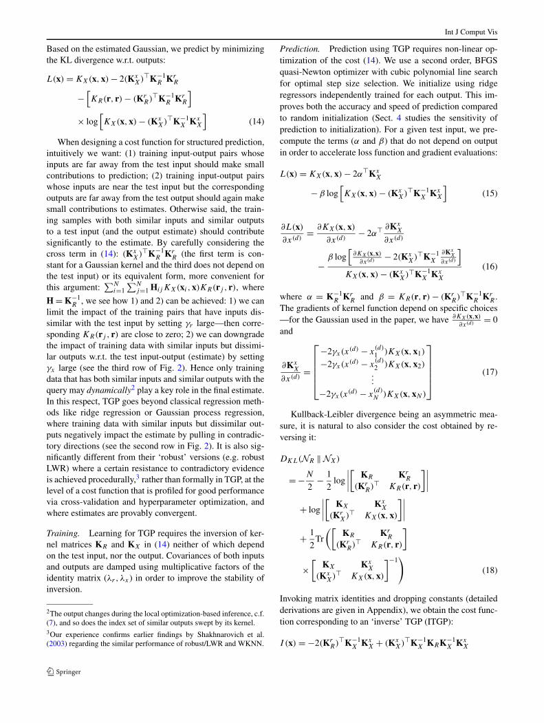
Fig. 1 Training set for a toy problem (predict a 1d output variablex given a 1d control r) consists of 250 values of x generated uni-formly in (0,1), for which we evaluate r = x + 0.3 sin(2xπ)+ ε with ε
drawn from a zero mean Gaussian with standard deviation 0.05. Starscorrespond to examples where KNN and GPR suffer from ‘bound-ary/discontinuous effects’. See also Fig. 2 for results that illustrate howdifferent models (KNN, GPR, TGP, ITGP) trained on this dataset be-have when tested with 250 equally spaced inputs r in (0,1)
+[KX(x,x) − (Kx
X)�K−1X Kx
X
]
× log[KX(x,x) − (Kx
X)�K−1X Kx
X
]
−[KX(x,x) − (Kx
X)�K−1X Kx
X
]
× log[KR(r, r) − (Kr
R)�K−1R Kr
R
](19)
Like TGP, we make predictions by optimizing (19) w.r.t. x.Intuitions behind different cost functions for both TGP
and ITGP are given next. Besides exploiting structured de-pendencies between outputs, TGP/ITGP give plausible solu-tions for ‘hard multivalue prediction problems’ where stan-dard regression methods such as GPR do not work well. Toillustrate, we consider a multivalued 1d input-output prob-lem, the S-shape (Bishop and Svensen 2003). In Fig. 1, wegenerate a training set of 250 values of x uniformly distrib-uted in (0,1) and evaluate r = x + 0.3 sin(2xπ) + ε withε drawn from a zero mean Gaussian with standard devi-ation 0.05. For testing, shown in Fig. 2, we generate 250equally-spaced values with x in (0,1) and evaluate r accord-ing to the model. The goal is to predict x given r , in thetest set according to the model learned based on the trainingset.
Although a toy problem, the S-shape models situationsthat occur in real world applications and datasets with mul-tivariate input-output samples, such as human pose recon-struction, because the output: 1) is multivalued in the mid-dle of S-shape; 2) is discontinuous on the boundary be-tween the univalued and multivalued regions, and 3) thetraining set is noisy. This epitomizes hard 3d from 2d articu-lated pose reconstruction problems from monocular images,
where ambiguities among multiple separated regions of thestate space (Sminchisescu and Triggs 2003) compound withrange uncertainty within each (Sminchisescu and Triggs2001), and persist even in restricted inference settings reg-ularized by temporal (dynamic) constraints (Sminchisescuand Jepson 2004b) or prior knowledge (Sminchisescu andJepson 2004a). Our experiments using complex image fea-tures and real vision datasets show that predictors like TGPor conditional mixture of experts models (BME and its vari-ants) consistently outperform GPR or KNN models—forcomplementary experiments see Sminchisescu et al. (2007),Bo et al. (2008).
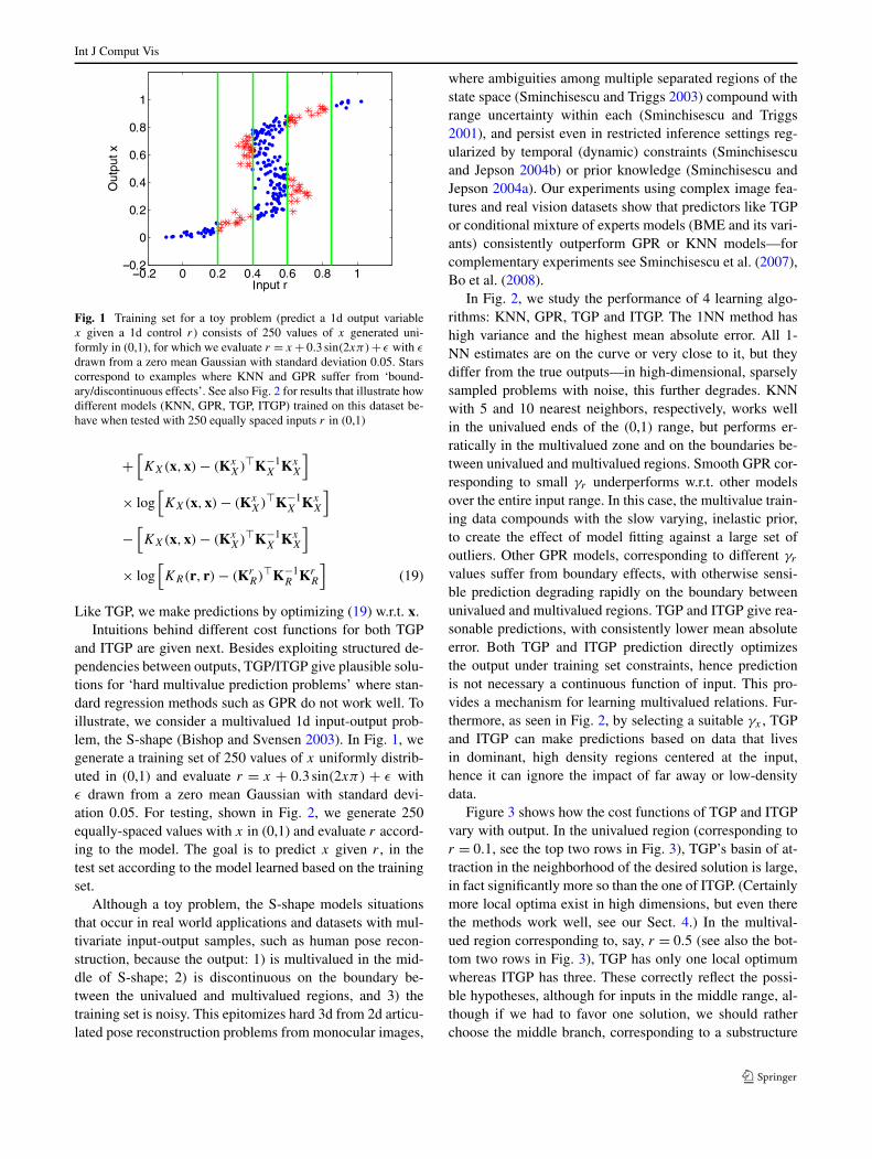
In Fig. 2, we study the performance of 4 learning algo-rithms: KNN, GPR, TGP and ITGP. The 1NN method hashigh variance and the highest mean absolute error. All 1-NN estimates are on the curve or very close to it, but theydiffer from the true outputs—in high-dimensional, sparselysampled problems with noise, this further degrades. KNNwith 5 and 10 nearest neighbors, respectively, works wellin the univalued ends of the (0,1) range, but performs er-ratically in the multivalued zone and on the boundaries be-tween univalued and multivalued regions. Smooth GPR cor-responding to small γr underperforms w.r.t. other modelsover the entire input range. In this case, the multivalue train-ing data compounds with the slow varying, inelastic prior,to create the effect of model fitting against a large set ofoutliers. Other GPR models, corresponding to different γr
values suffer from boundary effects, with otherwise sensi-ble prediction degrading rapidly on the boundary betweenunivalued and multivalued regions. TGP and ITGP give rea-sonable predictions, with consistently lower mean absoluteerror. Both TGP and ITGP prediction directly optimizesthe output under training set constraints, hence predictionis not necessary a continuous function of input. This pro-vides a mechanism for learning multivalued relations. Fur-thermore, as seen in Fig. 2, by selecting a suitable γx , TGPand ITGP can make predictions based on data that livesin dominant, high density regions centered at the input,hence it can ignore the impact of far away or low-densitydata.
Figure 3 shows how the cost functions of TGP and ITGPvary with output. In the univalued region (corresponding tor = 0.1, see the top two rows in Fig. 3), TGP’s basin of at-traction in the neighborhood of the desired solution is large,in fact significantly more so than the one of ITGP. (Certainlymore local optima exist in high dimensions, but even therethe methods work well, see our Sect. 4.) In the multival-ued region corresponding to, say, r = 0.5 (see also the bot-tom two rows in Fig. 3), TGP has only one local optimumwhereas ITGP has three. These correctly reflect the possi-ble hypotheses, although for inputs in the middle range, al-though if we had to favor one solution, we should ratherchoose the middle branch, corresponding to a substructure
Int J Comput Vis
Fig. 2 Prediction of KNN, Gaussian Process Regression (GPR) andTwin Gaussian Processes (TGP, ITPG) on the test set of the toy ex-ample described in Fig. 1. Err is mean absolute error. Top shows theprediction given by KNN for different number of neighbors, 1, 10 and20. Second row shows predictions of GPR with different kernel pa-rameters γr = 1, 5 and 10. Third row shows predictions of TGP with
different output kernel width parameters γx = 10, 15 and 20. Forth rowshows prediction given by ITGP with different kernel widths γx = 10,15 and 20 (width parameter γr is fixed at 0.2, cross-validated, for bothTGP and ITGP). The minima of ITGP tend to remain unchanged on theboundary between univalued and multivalued regions, hence predictionis flat there

Int J Comput Vis
Fig. 3 Costs of TGP and ITGP (14 and 19) as function of output x,for λr , λx = 10−4 and γr = 0.2. In the two top rows, input r is 0.1, forthe bottom two, r is 0.5. From left to right, γx is 10, 15, 20. The localoptima of TGP correspond to correct outputs for the different inputs
given (to check, use Fig. 1 to raise a vertical line at the query r andread the corresponding x values where this intercepts the S shape; seethe match with the minima of TGP/ITGP
with most nearby data support. This partly explains whyTGP is empirically found to be more reliable than ITGP forhuman pose reconstruction, although both work well in thetoy case.
2.3 Dynamic Twin Gaussian Processes (DTGP)
In sequence modeling or time series problems like track-ing, the state vectors link temporally, so the current state
Int J Comput Vis
not only correlates with the current image (observation),but often bears strong relation with previous states, in par-ticular the most recent. For non-linear dynamical systems,e.g. generative time-series models solved with Kalman fil-tering or particle filtering, the dependencies appear explic-itly in distributions p(xt |rt ) or p(xt |xt−1) (Bar-Shalom andFortman 1988; Isard and Blake 1998). For conditional timeseries models, the relations surface up as tertiary cliques,and recursive density propagation updates use local distrib-utions p(xt |xt−1, rt ) that bind together the reactive effectof measurements and correlations with the previous state(Sminchisescu et al. 2007). Here we take a cost break-down inspired by generative sequence models (but noticethat our search-based structured predictor integrates priorknowledge and search in a way that is very different fromgenerative models), and optimize the current state based notonly on TGP that correlate states and observations at thesame timestep, but also states at successive timesteps. Anal-ogous to how the dependencies are modeled in autoregres-sion (Bar-Shalom and Fortman 1988; Blake et al. 1999),we consider an auto-TGP. Without loss of generality, wework with a first-order auto-TGP, where the current stateis independent of all but the most recent one. Extensionsto multiple state dependencies are straightforward, althoughthey imply a more expensive optimization over state subse-quences larger than two timesteps, and are more sensitive tophase alignment of training and testing sequences.
Let Xt = (x2,x3, . . . ,xt ) be the joint set of states, includ-ing the current timestep t , where Xt stores the pose vec-tors columnwise. For notational compactness, we assumethe training set is temporally ordered. (For cases where thetraining set includes several sequences, the initial state X0 ofeach can be adjusted using an observation-sensitive TGP).Given Xt−1 and Xt as training inputs and outputs, the ideain auto-TGP is to predict the current state given the last stateusing TGP (the observation in the original TGP becomesthe state at the previous timestep in the supplementary auto-TGP term).
As for the TGP in the previous section, we specify a jointGaussian distribution over the training inputs and the testinput xt−1:
[(Xd
t−1)�
xdt−1
]∼ NXt−1
(
0,
[KXt−1 Kxt−1
Xt−1
(Kxt−1Xt−1
)� KXt−1(xt−1,xt−1)
])
(20)
Using the kernel function defined on outputs, we estimatethe covariance matrix
KXt
⋃xt
=[
KXt Kxt
Xt
(Kxt
Xt)� KXt (xt ,xt )
](21)
Again, we match the estimated covariance matrix of outputsto the one of inputs using Kullback-Leibler divergence. In-voking matrix identities and dropping constants, we mini-mize (22) with input xt−1 and output xt , as follows:
A(xt ,xt−1)
= KXt (xt ,xt ) − 2(Kxt
Xt)�K−1
Xt−1Kxt−1
Xt−1
+ (Kxt−1Xt−1
)�K−1Xt−1
KXt K−1Xt−1
Kxt−1Xt−1
−[KXt−1(xt−1,xt−1) − (Kxt−1
Xt−1)�K−1
Xt−1Kxt−1
Xt−1
]
× log[KXt (xt ,xt ) − (Kxt
Xt)�K−1
XtKxt
Xt
]
+[KXt−1(xt−1,xt−1) − (Kxt−1
Xt−1)�K−1
Xt−1Kxt−1
Xt−1
]
× log[KXt−1(xt−1,xt−1) − (Kxt−1
Xt−1)�K−1
Xt−1Kxt−1
Xt−1
]
(22)
Combining observation and dynamic components, we cre-ate a dynamic TGP (DTGP), which minimize the tradeoffbetween an observation-sensitive TGP and an auto-TGP:
D(x1,x2, . . . ,xT ) =T∑
t=1
L(xt ) + λ
T∑
t=1
A(xt ,xt−1) (23)
where λ ≥ 0 is a tradeoff parameter.One option is to optimize the cost sequentially, in a sweep
similar to filtering in non-linear, generative time-series mod-els (the cheapest option, computationally): at t = 1, only es-timate the state based on the observation sensitive TGP termof the cost (22). In subsequent steps fix xt−1 to the previ-ously estimated value and optimize the observation sensitiveand dynamic components of the cost w.r.t. xt . Other opti-mizations we have tried include the smoothed version wherext at all timesteps are estimated jointly, based on an entireobservation sequence, or a middle ground, where shorterstate subsequences are smoothed (we tested sequences ofsize 2, 5, 10, 15, 20, 30, 40 frames). All these more ex-pensive strategies improve the estimates to some degree, al-though in our experiments we found performance to saturatebeyond 20 timesteps.
Training. We need to compute matrices K−1R , K−1
Xt−1, K−1
Xt
and K−1Xt−1
KXt K−1Xt−1
, none depending either on the test inputor the test output. These account for temporal information inthe training set (damping factors λr , λxt−1 and λxt are used,in order to improve the stability of inversion).
Prediction. Like TGP, prediction of DTGP requires non-linear optimization over the desired number of timesteps.We work with the full DTGP (no KNN optimization, seenext section Sect. 2.4) and make predictions, once again, by
Int J Comput Vis
optimizing with a BFGS quasi-Newton method, with cubicpolynomial line search, and caching of output-independentmatrix blocks. DTGP-KNN is potentially more complex toimplement as nearest-neighbors of states being optimized,that forms the input to the pair-wise state auto-TGPs, changein a potentially non-smooth manner during optimization(we have obtained stable results using subgradient meth-ods). Initializing the state sequence using TGP (no dynamicconstraints, independent observation-based models at eachtime-step) often improves the speed of convergence andthe accuracy of prediction significantly compared to otherstrategies.
2.4 Twin Gaussian Process with K Nearest Neighbors
TGP requires N ×N matrix inversions with O(N3) trainingcost and O(N2) memory storage, which is impractical forproblems with more than 10,000 examples. Sparse approxi-mations can be used to reduce the training and storage costof TGP (Smola and Schölkopf 2000; Vincent and Bengio2002). The methods select a representative subset of regres-sors, dropping training complexity to O(Np2), where p isthe size of the subset. Since p�N in most cases, sparse ap-proximations achieve substantial speedups. They remain ap-plicable here, although a potential limitation is the indepen-dence of the representative subset from the run-time query.Another aspect is scaling to very large datasets where toachieve sufficiently accurate approximations even the sparsesubset can be too large.
Here, we adopt a conceptually simpler method: find theK nearest neighbors of a test input and estimate TGP on thereduced set (TGPKNN). A similar approach is widely usedin local regression (Schaal et al. 1997). The differences fromsparse approximations are worth noticing. Sparse methodsfind a reduced set globally, and this remains unchanged dur-ing testing. Instead, the working set of TGPKNN dependson the current test input. This allows us to work with a sig-nificantly smaller set that is potentially more relevant locallyand likely to generalize better. The trade-off is, as expected,in training vs. testing speed.
The naive version of KNN is easy to implement (com-pute distances between a test and all training inputs), butcomputationally intensive for large datasets. Many sophis-ticated NN search algorithms have been proposed, gen-erally seeking to reduce the number of distance evalua-tions performed. Recent work (Krauthgamer and Lee 2004;Cortes et al. 2005) shows that the cost of K nearest neigh-bor queries can be driven down to O(log(N)) if cover treedata structures are used. We follow this to drop the compu-tational cost of TGPKNN to O(log(N))+ O(K3), where K
is constant (in our experiments, K = 1000 worked just fine).Hence, TGPKNN has potential for large training sets in theorder of 108 examples.
3 Kernel Target Alignment and Hilbert-SchmidtIndependence Criterion
An alternative interpretation is to view the Kullback-Leiblerdivergence as one possible kernel dependency measure thatgives the goodness of alignment between two kernels. Thisraises the question whether other kernel dependency mea-sures can work better than KL for prediction. Kernel Tar-get Alignment (KTA) (Cristianini et al. 2001a, 2001b) is awidely used measure that has been applied to kernel para-meter optimization, feature selection, clustering, etc. KTAwrites as follows:
KTA = Tr(KRX�X)√
Tr(KRKR)Tr(X�XX�X)(24)
where KR is the kernel matrix defined over inputs and X isthe output. Although the original KTA does not use a non-linear kernel on outputs, one can, in principle replace X�Xby KX:
KTA = Tr(KRKX)√Tr(KRKR)Tr(KXKX)
(25)
Like in the previous section, consider the two kernel ma-trices defined over an augmented set consisting of a train-
ing set, a test input and its target output:[ KR Kr
R
(KrR)� KR(r,r)
]and
[ KX KxX
(KxX)� KX(x,x)
]. Substituting into (25), we obtain
KTA = Tr(KRKX) + 2(KrR)�Kx
X + KR(r, r)KX(x,x)√
Tr(KXKX) + 2(KxX)�Kx
X + KX(x,x)KX(x,x)
(26)
where we dropped the constant term:
√Tr(KRKR) + 2(Kr
R)�KrR + KR(r, r)KR(r, r) (27)
Prediction is made by maximizing (26) with respect to x.Another potentially relevant alignment method is the
Hilbert-Schmidt Independence Criterion (HSIC) (Gretton etal. 2005a, 2005b). This has the form:
HISC = (N − 1)2Tr(KXHNKRHN) (28)
where HN = IN − 1N
N, IN is an N × N identity matrix and
1N is an N × N matrix of all 1s. We consider an augmentedset (training set, test input and target output):
HSIC = N2[Tr(KRKX) + 2(K
r
R)�KxX
+ KR(r, r)KX(x,x)]
(29)
Int J Comput Vis
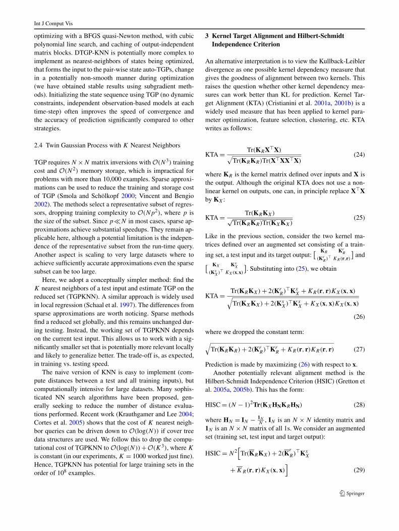
Fig. 4 Prediction of kernel target alignment and Hilbert-Schmidt inde-pendent criterion on the test set of the toy problem described in Fig. 1.Err is the mean absolute error. Top row shows the prediction given by
KTA with width parameters γx = 30, 40, 50. Bottom row gives HSICpredictions for widths γx = 10, 15, 20. The parameter γr is cross-validated to 5 and 0.2 for KTA and HSIC, respectively
where
[KR K
r
R
(Kr
R)� KR(r, r)
]
= HN+1
[KR Kr
R
(KrR)� KR(r, r)
]HN+1
(30)
Figure 4 shows predictive results of KTA and HSIC onthe toy problem described in Fig. 1. Like TGP, KTA andHSIC can deal with discontinued, multivalued regimes (theprediction can change abruptly on the boundary betweenunivalued and multivalued regions) although KTA and HSICappear to be less accurate than TGP. Our experiments forhuman motion reconstruction in Sect. 4 suggest that TGPis significantly more accurate than KTA and HSIC. TGP isclosely related to Gaussian processes which are successfulpredictors for standard cases, whereas algorithms like KTAor HSIC were primarily designed for parameter selection orindependence testing, not for prediction. For instance, thecost function of HSIC is not necessarily maximized whenthe two kernel matrices are identical, which makes predic-tion by HSIC somewhat inaccurate even in regions wherethere are consistently single solutions.
4 Experiments
We evaluate the performance of TGP and its variants on theHumanEva-I dataset (Sigal and Black 2006), which consistsof 4 subjects doing 6 predefined actions: Walking, Jogging,Throw-catch, Gestures, Boxing and Combo (walking fol-lowed by jogging and then balancing on each one of thetwo feet). Video data and ground truth motion of the bodyare captured using a marker-based motion capture systemand synchronized in software. Combo motions of all sub-jects and all motions of one subject are withheld. Table 1summarizes the structure of the training set (frames with in-valid MoCap were removed). For details on HumanEva, seethe report by the authors (Sigal and Black 2006). For someof the experiments we use image features extracted fromthe first camera, together with additional training samplesobtained from the second and the third camera, using vir-tual rotations of their pose sets into one common monocularframe (Poppe 2007). In this way we triple the ‘monocular’training set (rather than triple the descriptor size). Modelsobtained in this way are referred in our tables as ‘C1Add’.We also run (truly) monocular experiments where only datafrom one camera is used, e.g. ‘C1’. In other experiments,image features extracted of images from 3 cameras are com-bined in a (longer 3×) descriptor, ‘C1+C2+C3’.
Int J Comput Vis
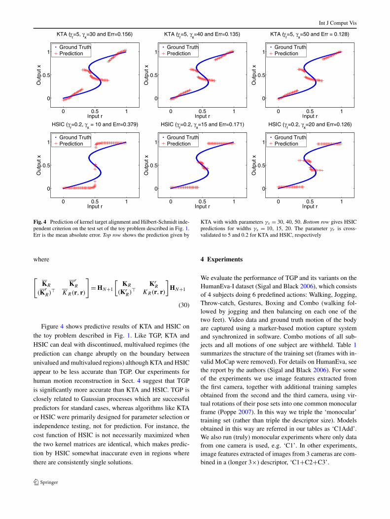
Fig. 5 Affinity matrices fordifferent motions executed bySubject 2 in HumanEva. Thesecorrespond to features extractedfrom images of the first camera,on temporally ordered testsequences, and are computedbased on the Euclidean distancebetween image features (darkermeans more similar). The firstand third columns showaffinities for HMAX, the secondand fourth for HoG. From top tobottom: Walking, Jogging andGesture sequences
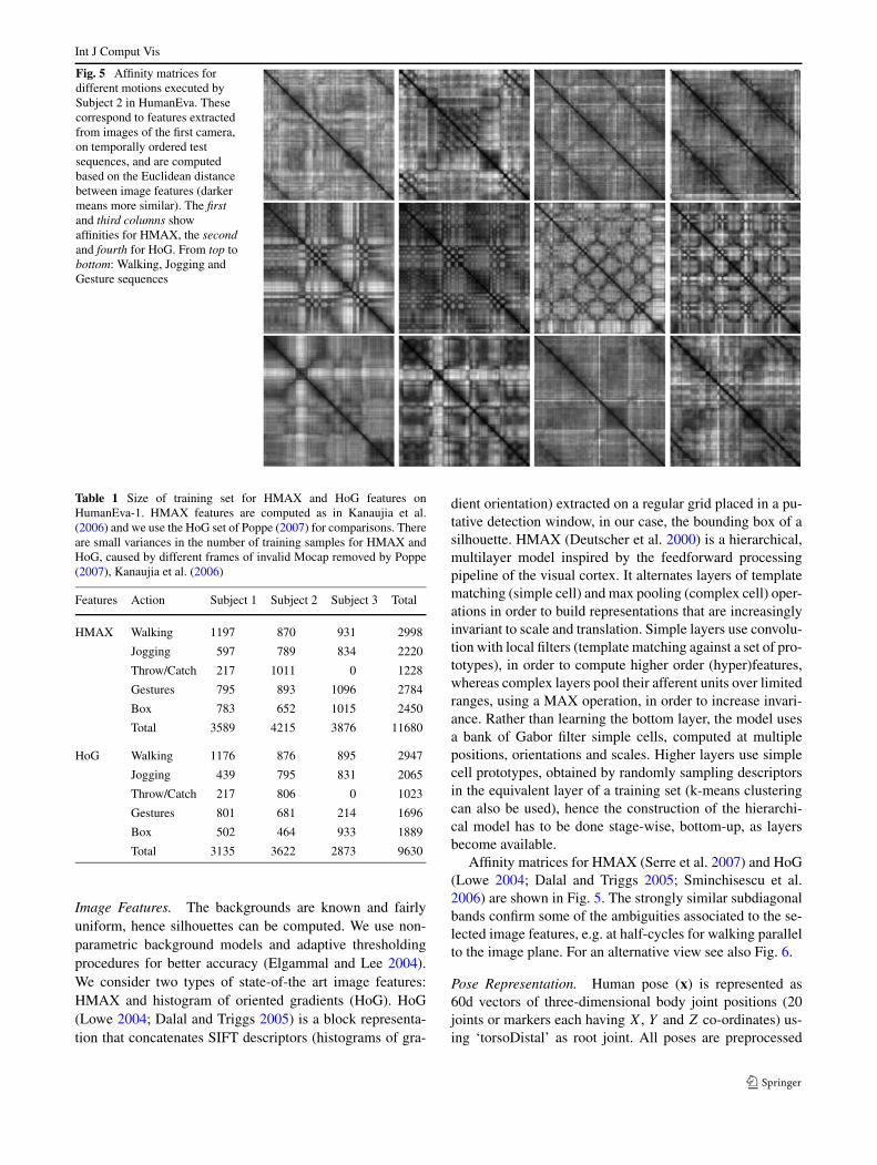
Table 1 Size of training set for HMAX and HoG features onHumanEva-1. HMAX features are computed as in Kanaujia et al.(2006) and we use the HoG set of Poppe (2007) for comparisons. Thereare small variances in the number of training samples for HMAX andHoG, caused by different frames of invalid Mocap removed by Poppe(2007), Kanaujia et al. (2006)
Features Action Subject 1 Subject 2 Subject 3 Total
HMAX Walking 1197 870 931 2998
Jogging 597 789 834 2220
Throw/Catch 217 1011 0 1228
Gestures 795 893 1096 2784
Box 783 652 1015 2450
Total 3589 4215 3876 11680
HoG Walking 1176 876 895 2947
Jogging 439 795 831 2065
Throw/Catch 217 806 0 1023
Gestures 801 681 214 1696
Box 502 464 933 1889
Total 3135 3622 2873 9630
Image Features. The backgrounds are known and fairlyuniform, hence silhouettes can be computed. We use non-parametric background models and adaptive thresholdingprocedures for better accuracy (Elgammal and Lee 2004).We consider two types of state-of-the art image features:HMAX and histogram of oriented gradients (HoG). HoG(Lowe 2004; Dalal and Triggs 2005) is a block representa-tion that concatenates SIFT descriptors (histograms of gra-
dient orientation) extracted on a regular grid placed in a pu-tative detection window, in our case, the bounding box of asilhouette. HMAX (Deutscher et al. 2000) is a hierarchical,multilayer model inspired by the feedforward processingpipeline of the visual cortex. It alternates layers of templatematching (simple cell) and max pooling (complex cell) oper-ations in order to build representations that are increasinglyinvariant to scale and translation. Simple layers use convolu-tion with local filters (template matching against a set of pro-totypes), in order to compute higher order (hyper)features,whereas complex layers pool their afferent units over limitedranges, using a MAX operation, in order to increase invari-ance. Rather than learning the bottom layer, the model usesa bank of Gabor filter simple cells, computed at multiplepositions, orientations and scales. Higher layers use simplecell prototypes, obtained by randomly sampling descriptorsin the equivalent layer of a training set (k-means clusteringcan also be used), hence the construction of the hierarchi-cal model has to be done stage-wise, bottom-up, as layersbecome available.
Affinity matrices for HMAX (Serre et al. 2007) and HoG(Lowe 2004; Dalal and Triggs 2005; Sminchisescu et al.2006) are shown in Fig. 5. The strongly similar subdiagonalbands confirm some of the ambiguities associated to the se-lected image features, e.g. at half-cycles for walking parallelto the image plane. For an alternative view see also Fig. 6.
Pose Representation. Human pose (x) is represented as60d vectors of three-dimensional body joint positions (20joints or markers each having X, Y and Z co-ordinates) us-ing ‘torsoDistal’ as root joint. All poses are preprocessed

Int J Comput Vis
Fig. 6 Ambiguities in HumaEva-I. We select a test image according to the motion shown in the title and find its 50 nearest neighbors based onHoG. We record 3d poses associated with the 50 images and plot the Euclidean distance between the pose of the nearest image and the other 49poses (notice that no ground truth is used, as we don’t have it). Notice that poses cluster at multiple well separated levels
by subtracting the root joint location from all the other jointpositions in every frame. This representation is not partic-ularly good for learning, as perceptually identical poses ofpeople with different body proportions tend to be encodedsomewhat differently (joint angles and skeletons could havebeen more appropriate, but they are not currently availablefor HumanEva), but our normalization by root subtractionappears to largely palliate this. In fact, it turns out that TGPis not sensitive to different body proportions or the existenceof accurate kinematic or volumetric human body models:methods trained on samples captured from all subjects donot perform significantly worse than those trained on indi-vidual subjects (see our Tables 4 and 5). This degree of ro-bustness is harder to achieve with a generative model wherealignment (observation modeling) constraints pay an impor-tant role, and reliable inference is often contingent both ona 3d human model well adapted to the body proportionsof each human subject and on good camera calibration, setaside model initialization. These stringent requirements areno longer required for TGP.
Error Metric. We report the error between the estimated xand the ground truth pose x according to the measure sug-gested by Sigal and Black (Sigal and Black 2006), and usedby the online evaluation system:
D(x,x) = 1
M
M∑
i=1
‖mi(x) − mi(x)‖ (31)
where mi(x) ∈ R3 is a function that extracts the three dimen-
sional coordinates of the ith joint position, M is the numberof the joint positions for each pose and ‖ · ‖ is the Euclideandistance. For a motion sequence of T frames, we report theaverage joint position error as:
Errseq = 1
T
T∑
i=1
D(xi ,xi ) (32)
4.1 Initialization of TGP
For pose estimation, TGP optimizes a non-convex cost func-tion (14), and a suitable initialization is desirable in order toavoid shallow local optima. We study the impact of three dif-ferent initialization methods: K nearest neighbors (KNN),ridge regression (RR) with models trained for each outputdimension independently and ground truth (GrTruth), whichwe don’t have in general, but represents a gold standard tocheck against model bias. In this experiment we use the val-idation set as test set, but for methodological consistency wedivide each train and validation sequence into approximatelyequal chunks. The new ‘training and validation set’ consistsof the second half of all motions sequences from all subjectsand the new ‘test set’ consists of their first half.
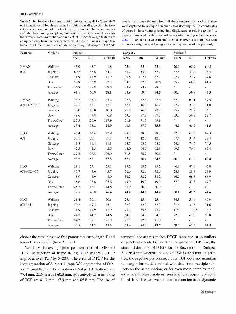
We set λr = λx = 10−4 (inversion of kernel matrices isinvolved in TGP and mild damping with a multiplicativefactor of a diagonal matrix improves stability), and to cross-validate we grid search for γr and γx over suitable ranges.The results are shown in Table 2. As expected, ground truthinitialization works best among all three methods. RR out-performs KNN in most cases with estimates based on RRclose to the ones obtained from ground truth. For example,for HoG (C1+C2+C3), RR initialization gives the same av-erage error as the ground truth for Subjects 2 and 3, and only0.4 mm higher average error for Subject 1.
4.2 Evaluation of Dynamic TGP
This section compares the static and dynamic versions ofTGP. We initialize TGP using independent output RR andoptimize the kernel parameters γr and γx using cross vali-dation. We initialize DTGP with the estimated pose of theobservation-sensitive TGP, obtained independently, at eachtimestep—this usually gives good starting points and accel-erates convergence. The observation-dependent componentof DTGP is set as in the static model (TGP) and the ker-nel parameter of the dynamic, auto-TGP, γA is set to γx . We
Int J Comput Vis
Table 2 Evaluation of different initializations using HMAX and HoGon HumanEva-I. Models are trained on data from all subjects. The low-est error is shown in bold. In the table, ‘/’ show that the values are notavailable (no training samples); ‘Average’ gives the averaged error forthe different motions of the same subject; ‘C1’ means image feature arecomputed only from the first camera; ‘C1+C2+C3’ means image fea-tures from three cameras are combined in a single descriptor; ‘C1Add’
means that image features from all three cameras are used as if theywere captured by a single camera by transforming the 3d coordinatesof poses in those cameras using their displacements relative to the firstcamera, thus tripling the standard monocular training set size (Poppe2007). KNN, RR and GrTruth indicate that TGPKNN is initialized withK nearest neighbors, ridge regression and ground truth, respectively
Features Motions Subject 1 Subject 2 Subject 3
KNN RR GrTruth KNN RR GrTruth KNN RR GrTruth
HMAX Walking 43.9 43.7 41.8 25.4 25.4 25.4 70.9 68.9 64.5
(C1) Jogging 60.2 57.6 54.7 53.7 53.2 52.7 37.5 37.4 36.4
Gestures 11.9 11.9 11.9 100.8 102.1 87.3 27.7 27.7 27.8
Box 52.9 52.9 52.7 104.5 82.5 78.6 65.2 68.9 61.4
ThrowCatch 136.8 137.8 129.5 89.9 83.9 78.7 / / /
Average 61.1 60.9 58.1 74.9 69.4 64.5 50.3 50.7 47.5
HMAX Walking 33.2 33.2 33.2 22.6 22.6 22.6 67.4 61.1 57.5
(C1+C2+C3) Jogging 47.1 47.1 47.1 47.1 46.9 46.7 32.7 31.9 31.8
Gestures 10.0 10.0 10.0 96.5 86.4 82.2 25.9 25.7 24.1
Box 49.6 49.8 46.8 63.2 57.8 57.5 53.5 56.8 52.7
ThrowCatch 127.3 126.0 117.9 71.9 71.3 69.9 / / /
Average 53.4 53.2 51.0 60.3 57.0 55.8 44.9 43.9 41.5
HoG Walking 45.4 43.4 42.9 28.3 28.3 28.3 62.3 62.5 62.3
(C1) Jogging 55.1 55.1 55.1 43.2 42.5 42.5 37.4 37.4 37.4
Gestures 11.8 11.8 11.8 68.7 68.3 68.3 74.6 74.5 74.5
Box 42.5 42.5 42.5 64.0 64.0 62.8 69.3 70.4 67.4
ThrowCatch 137.8 137.8 136.9 81.5 78.7 70.6 / / /
Average 58.5 58.1 57.8 57.1 56.4 54.5 60.9 61.2 60.4
HoG Walking 29.1 29.1 29.1 19.2 19.2 19.2 46.8 47.0 46.8
(C1+C2+C3) Jogging 43.7 43.6 43.7 32.6 32.6 32.6 28.9 28.9 28.9
Gestures 8.9 8.9 8.9 58.2 58.2 58.2 66.9 66.8 66.9
Box 35.6 35.6 35.6 49.9 49.9 49.9 57.9 47.8 47.7
ThrowCatch 145.2 116.7 114.8 60.9 60.9 60.9 / / /
Average 52.5 46.8 46.4 44.2 44.2 44.2 50.1 47.6 47.6
HoG Walking 31.4 30.8 30.6 25.4 25.4 25.4 54.5 51.4 49.9
(C1Add) Jogging 50.2 49.5 45.1 32.3 32.3 32.3 31.6 31.6 31.6
Gestures 11.9 11.9 11.9 75.7 75.8 75.7 119.2 118.2 78.7
Box 44.7 44.7 44.6 64.7 64.3 64.3 72.3 67.6 59.8
ThrowCatch 134.2 137.1 125.9 76.5 72.5 71.0 / / /
Average 54.5 54.8 51.6 54.9 54.0 53.7 69.4 67.2 55.4
choose the remaining two free parameters: step length T andtradeoff λ using CV (here T = 20).
We show the average joint position error of TGP andDTGP as function of frame in Fig. 7. In general, DTGPimproves over TGP by 5–20%. The error of DTGP for theJogging motion of Subject 1 (top), Walking motion of Sub-ject 2 (middle) and Box motion of Subject 3 (bottom) are77.4 mm, 22.6 mm and 60.5 mm, respectively whereas thoseof TGP are 81.3 mm, 27.9 mm and 65.8 mm. The use of
temporal constraints makes DTGP more robust to outliersor poorly segmented silhouettes compared to TGP. E.g., thestandard deviation of DTGP for the Box motion of Subject3 is 26.4 mm whereas the one of TGP is 52.5 mm. In prac-tice, the superior performance over TGP does not maintainits margin for models trained with data from multiple sub-jects on the same motion, or for even more complex mod-els where different motions from multiple subjects are com-bined. In such cases, we notice an attenuation in the dynamic
Int J Comput Vis
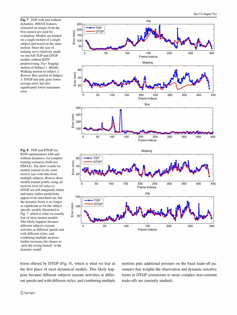
Fig. 7 TGP with and withoutdynamics. HMAX featuresextracted on images from thefirst camera are used forevaluation. Models are trainedon a single motion of a singlesubject and tested on the samemotion. Since the size oftraining set is relatively small,we run full TGP and DTGPmodels without KNNpreprocessing. Top: Joggingmotion of Subject 1. Middle:Walking motion of subject 2.Bottom: Box motion of Subject3. DTGP not only gives loweraverage error, but alsosignificantly lower maximumerror
Fig. 8 TGP and DTGP (noKNN optimization) with andwithout dynamics, for complextraining scenarios (both useHMAX). Top show results formodels trained on the samemotion type with data frommultiple subjects. Bottom showmodels trained jointly using allmotions from all subjects.DTGP are still marginally betterand many outlier predictionsappear to be smoothed out, butthe dynamic boost is no longeras significant as for the subjectspecific models illustrated inFig. 7, which is what we usuallyfear of most motion models.This likely happens becausedifferent subjects executeactivities at different speeds andwith different styles, andcombining multiple motionsfurther increases the chance to‘pick the wrong branch’ in thedynamic model
boost offered by DTGP (Fig. 8), which is what we fear in
the first place of most dynamical models. This likely hap-
pens because different subjects execute activities at differ-
ent speeds and with different styles, and combining multiple
motions puts additional pressure on the fixed trade-off pa-
rameter that weights the observation and dynamic-sensitive
terms in DTGP (extensions to more complex non-constant
trade-offs are currently studied).
Int J Comput Vis
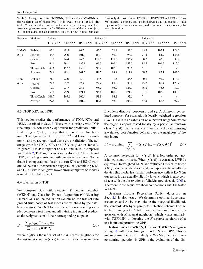
Table 3 Average errors for ITGPKNN, HSICKNN and KTAKNN onthe validation set of HumanEva-I, with lowest error in bold. In thetable, ‘/’ marks values that are not available (no training samples);‘Average’ gives average error for different motions of the same subject;‘C1’ indicates that models are trained only with HoG features extracted
form only the first camera. ITGPKNN, HSICKNN and KTAKNN use800 nearest neighbors, and are initialized using the output of ridgeregression (RR) with univariate predictors trained independently foreach dimension
Features Motions Subject 1 Subject 2 Subject 3
ITGPKNN KTAKNN HSICKNN ITGPKNN KTAKNN HSICKNN ITGPKNN KTAKNN HSICKNN
HMAX Walking 67.6 89.5 90.7 47.7 71.8 82.0 85.7 102.1 124.2
(C1) Jogging 84.4 95.0 101.0 83.3 95.7 94.2 71.4 84.9 134.6
Gestures 13.0 24.4 26.7 117.9 118.9 136.4 30.3 43.8 39.2
Box 64.6 79.1 132.1 99.3 106.1 153.5 85.5 101.7 112.0
ThrowCatch 143.6 152.6 156.8 95.4 102.1 93.6 / / /
Average 74.6 88.1 101.5 88.7 98.9 111.9 68.2 83.1 102.5
HoG Walking 71.7 92.0 95.1 46.5 76.8 85.5 80.2 95.9 116.7
(C1) Jogging 72.6 82.7 97.5 72.4 89.3 93.2 73.2 86.4 123.4
Gestures 12.3 23.7 25.8 95.2 95.0 126.9 36.2 45.5 39.3
Box 55.8 75.9 121.1 96.8 108.7 121.7 81.8 102.2 109.3
ThrowCatch 149.7 163.8 166.4 91.8 98.8 92.6 / / /
Average 72.4 87.6 101.2 80.5 93.7 104.0 67.9 82.5 97.2
4.3 ITGP, KTA and HSIC
This section studies the performance of ITGP, KTA andHSIC, described in Sect. 3. These work similarly with TGP(the output is non-linearly optimized for prediction, initial-ized using RR, etc.), except that different cost functionsused. The regularizers λr = λx = 10−4 and kernel parame-ters γr and γx are optimized using cross validation. The av-erage error for ITGP, KTA and HSIC is given in Table 3.In general, ITGP is superior to KTA and HSIC. Comparedwith Table 2, TGP significantly outperforms ITGP, KTA andHSIC, a finding consistent with our earlier analysis. Noticethat it is computational feasible to run KTA and HSIC with-out KNN, but our experience suggests that combining KTAand HSIC with KNN gives lower errors compared to modelstrained on the full dataset.
4.4 Evaluation of TGP
We compare TGP with weighted K nearest neighbor(WKNN) and Gaussian Process Regression (GPR), usingHumanEva’s online evaluation system on the test set (theground truth poses of test videos are withheld by the data-base creators). WKNN locates the K closest training sam-ples between a test input and all training inputs and predictsas the weighted sum of their corresponding outputs:
x∗ =∑
j∈Nk(r) W(r, rj )xj∑
j∈Nk(r) W(r, rj )(33)
where Nk(r) is the index set of the K nearest neighbors forthe test input r and W(r, rj ) is the similarity measure (here
Euclidean distance) between r and rj . A different, yet re-lated approach for estimation is locally weighted regression(LWR). LWR is an extension of K nearest neighbors wherethe target is approximated locally by a particular functionclass f (r;β). The parameters β are learned by minimizinga weighted cost function defined over the neighbors of thetest input:
β∗r = argminβr
∑
j∈Nk(r)
W(r, rj )‖xj − f (rj ;βr)‖2 (34)
A common selection for f (r;β) is a low-order polyno-mial, constant or linear. When f (r;β) is constant, LWR isequivalent to weighted KNN. We evaluated LWR with linearf (r;β) on the validation set and our experimental results in-dicated this model has similar performance with WKNN (inour tests, it was actually slightly lower), which is also con-sistent with the observations of Shakhnarovich et al. (2003).Therefore in the sequel we show comparisons with the fasterWKNN.
Gaussian Process Regression (GPR), described inSect. 2.1 is also tested. We determine optimal hyperpara-meters γr and λr by maximizing the marginal likelihood,the standard GPR hyperparameter selection scheme. For thetripled training set (C1Add), we use Gaussian process re-gression with K nearest neighbors, which works similarlywith TGPKNN, by locating the K nearest neighbors of atest input and performing GPR.
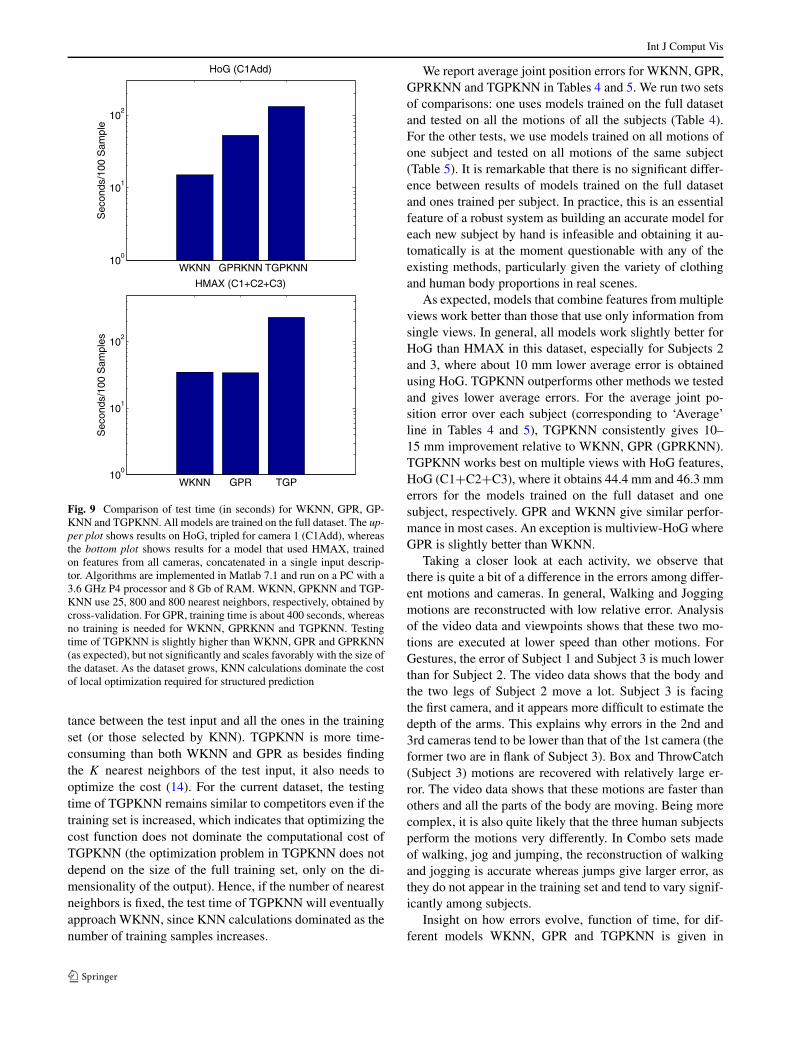
Testing times for WKNN, GPR and TGPKNN are givenin Fig. 9, with close timings of WKNN and GPR. This isnot surprising because similarly to WKNN, the most time-consuming operation in GPR is the evaluation of the dis-
Int J Comput Vis
Fig. 9 Comparison of test time (in seconds) for WKNN, GPR, GP-KNN and TGPKNN. All models are trained on the full dataset. The up-per plot shows results on HoG, tripled for camera 1 (C1Add), whereasthe bottom plot shows results for a model that used HMAX, trainedon features from all cameras, concatenated in a single input descrip-tor. Algorithms are implemented in Matlab 7.1 and run on a PC with a3.6 GHz P4 processor and 8 Gb of RAM. WKNN, GPKNN and TGP-KNN use 25, 800 and 800 nearest neighbors, respectively, obtained bycross-validation. For GPR, training time is about 400 seconds, whereasno training is needed for WKNN, GPRKNN and TGPKNN. Testingtime of TGPKNN is slightly higher than WKNN, GPR and GPRKNN(as expected), but not significantly and scales favorably with the size ofthe dataset. As the dataset grows, KNN calculations dominate the costof local optimization required for structured prediction
tance between the test input and all the ones in the trainingset (or those selected by KNN). TGPKNN is more time-consuming than both WKNN and GPR as besides findingthe K nearest neighbors of the test input, it also needs tooptimize the cost (14). For the current dataset, the testingtime of TGPKNN remains similar to competitors even if thetraining set is increased, which indicates that optimizing thecost function does not dominate the computational cost ofTGPKNN (the optimization problem in TGPKNN does notdepend on the size of the full training set, only on the di-mensionality of the output). Hence, if the number of nearestneighbors is fixed, the test time of TGPKNN will eventuallyapproach WKNN, since KNN calculations dominated as thenumber of training samples increases.
We report average joint position errors for WKNN, GPR,GPRKNN and TGPKNN in Tables 4 and 5. We run two setsof comparisons: one uses models trained on the full datasetand tested on all the motions of all the subjects (Table 4).For the other tests, we use models trained on all motions ofone subject and tested on all motions of the same subject(Table 5). It is remarkable that there is no significant differ-ence between results of models trained on the full datasetand ones trained per subject. In practice, this is an essentialfeature of a robust system as building an accurate model foreach new subject by hand is infeasible and obtaining it au-tomatically is at the moment questionable with any of theexisting methods, particularly given the variety of clothingand human body proportions in real scenes.
As expected, models that combine features from multipleviews work better than those that use only information fromsingle views. In general, all models work slightly better forHoG than HMAX in this dataset, especially for Subjects 2and 3, where about 10 mm lower average error is obtainedusing HoG. TGPKNN outperforms other methods we testedand gives lower average errors. For the average joint po-sition error over each subject (corresponding to ‘Average’line in Tables 4 and 5), TGPKNN consistently gives 10–15 mm improvement relative to WKNN, GPR (GPRKNN).TGPKNN works best on multiple views with HoG features,HoG (C1+C2+C3), where it obtains 44.4 mm and 46.3 mmerrors for the models trained on the full dataset and onesubject, respectively. GPR and WKNN give similar perfor-mance in most cases. An exception is multiview-HoG whereGPR is slightly better than WKNN.
Taking a closer look at each activity, we observe thatthere is quite a bit of a difference in the errors among differ-ent motions and cameras. In general, Walking and Joggingmotions are reconstructed with low relative error. Analysisof the video data and viewpoints shows that these two mo-tions are executed at lower speed than other motions. ForGestures, the error of Subject 1 and Subject 3 is much lowerthan for Subject 2. The video data shows that the body andthe two legs of Subject 2 move a lot. Subject 3 is facingthe first camera, and it appears more difficult to estimate thedepth of the arms. This explains why errors in the 2nd and3rd cameras tend to be lower than that of the 1st camera (theformer two are in flank of Subject 3). Box and ThrowCatch(Subject 3) motions are recovered with relatively large er-ror. The video data shows that these motions are faster thanothers and all the parts of the body are moving. Being morecomplex, it is also quite likely that the three human subjectsperform the motions very differently. In Combo sets madeof walking, jog and jumping, the reconstruction of walkingand jogging is accurate whereas jumps give larger error, asthey do not appear in the training set and tend to vary signif-icantly among subjects.
Insight on how errors evolve, function of time, for dif-ferent models WKNN, GPR and TGPKNN is given in

Int J Comput Vis
Table 4 Evaluation of average joint position error (and variance) ofdifferent models that use input descriptors based on HMAX and HoGon the test set of HumanEva-I (error reported in mm). All models aretrained jointly on data from the three human subjects. Average jointposition error is computed by Humaneva’s online evaluation system,and we discard frames with invalid mocap case when the evaluationsystem returns −1 (note that averages become lower if values for in-valid frames are taken to be 0). The lowest error is given in bold. Inthe table, ‘/’ indicates that the values are not available (for whateverreason no test results are returned); ‘Average’ gives the average er-
ror for the different motions of the same subject; ‘C1’ indicates thatimage features are computed only using data from the first camera;‘C1+C2+C3’ means that image features from three cameras are com-bined in a single descriptor; ‘C1Add’ means that data from the firstcamera is augmented with data from the second and third by trans-forming to the coordinate system of the first. We used GPR with KNNfor the tripled training samples (standard GPR wouldn’t work becausethere are too many training samples). WKNN, GPRKNN and TGP-KNN use 25, 800 and 800 neighbors, respectively, all cross-validated
Features Motions Subject 1 Subject 2 Subject 3
WKNN GPR TGPKNN WKNN GPR TGPKNN WKNN GPR TGPKNN
HMAX Walking 45.9(22.6) 65.3(22.3) 37.5(17.0) 48.2(25.5) 60.2(19.2) 40.2(17.8) 63.8(23.6) 74.4(27.9) 51.1(27.1)
(C1) Jogging 55.9(21.0) 69.6(19.8) 48.7(17.7) 56.4(22.6) 66.6(19.0) 46.5(15.3) 68.3(27.2) 82.2(22.0) 58.9(21.1)
Gestures 25.7(5.7) 30.8(6.7) 22.3(4.1) 93.3(30.9) 103.9(20.5) 84.5(16.1) 75.9(26.7) 68.5(9.9) 54.3(11.2)
Box 73.6(14.3) 90.8(15.6) 79.6(23.4) 130.7(60.6) 133.4(54.6) 122.6(59.5) 112.1(48.1) 135.7(46.0) 116.9(64.9)
ThrowCatch / / / 74.5(35.3) 70.4(26.9) 67.5(32.1) 124.5(36.9) 78.3(21.7) 112.7(34.6)
Combo / / / 87.6(61.6) 90.1(45.6) 74.1(53.3) 131.7(88.9) 125.2(63.3) 116.1(77.4)
Average 50.3 64.1 47.0 81.7 87.4 72.6 96.0 94.1 85.0
HMAX Walking 41.5(15.5) 53.0(17.0) 31.3(7.2) 47.2(30.4) 44.8(15.5) 32.2(15.3) 46.2(21.7) 56.1(19.5) 35.3(16.3)
(C1+C2+C3) Jogging 52.1(18.7) 49.8(12.2) 37.1(9.1) 44.3(15.2) 47.8(12.5) 34.6(7.4) 52.3(22.3) 60.6(18.6) 42.7(15.7)
Gestures 24.3(7.4) 28.0(5.8) 21.6(5.2) 84.0(22.3) 86.1(17.0) 68.7(15.7) 49.6(6.1) 55.3(6.9) 46.5(4.7)
Box 86.8(46.3) 74.2(22.6) 81.7(36.3) 112.1(56.6) 108.5(53.0) 89.7(42.9) 93.4(37.4) 131.6(44.1) 92.8(51.6)
ThrowCatch / / / 69.2(33.5) 70.4(26.9) 53.2(22.9) 114.1(35.9) 66.4(24.9) 90.2(33.6)
Combo / / / 82.3(53.4) 73.5(44.8) 62.3(50.0) 91.9(49.3) 110.7(53.3) 81.4(49.1)
Average 51.2 51.3 42.9 73.1 71.9 56.8 74.6 78.5 64.8
HoG Walking 47.5(21.1) 62.1(25.9) 38.2(21.4) 46.7(35.2) 51.1(30.0) 32.8(23.1) 66.7(32.0) 58.2(25.2) 40.2(23.2)
(C1) Jogging 54.5(22.4) 64.4(21.1) 42.0(12.9) 43.3(14.4) 51.9(22.7) 34.7(16.6) 56.1(25.4) 66.6(28.0) 46.4(28.9)
Gestures 23.4(13.5) 26.8(11.2) 20.4(7.6) 75.1(28.1) 85.5(21.8) 71.7(25.7) 75.3(11.1) 75.3(11.5) 72.7(21.2)
Box 79.7(27.7) 78.3(21.7) 63.1(14.2) 105.8(46.9) 100.3(46.2) 98.6(64.1) 100.4(52.3) 117.7(43.7) 106.7(62.6)
ThrowCatch / / / 71.4(34.2) 78.6(22.6) 52.6(25.8) 111.7(32.9) 68.1(21.8) 107.5(38.2)
Combo / / / 78.6(48.6) 83.8(50.5) 66.5(61.2) 114.0(77.3) 122.6(80.2) 95.3(75.6)
Average 51.3 57.9 40.9 70.1 75.2 59.5 87.4 84.8 78.1
HoG Walking 37.5(12.0) 45.1(21.0) 26.6(7.0) 40.1(23.9) 33.5(15.1) 25.2(9.7) 55.3(25.1) 42.3(20.7) 31.0(13.3)
(C1+C2+C3) Jogging 45.2(13.7) 43.1(14.4) 32.2(9.1) 37.7(12.2) 31.4(9.2) 26.9(6.0) 45.4(18.3) 42.6(14.3) 32.4(10.5)
Gestures 23.7(7.2) 27.7(7.4) 19.2(3.5) 72.8(26.3) 67.6(17.8) 50.2(11.2) 56.1(6.4) 48.6(5.2) 50.9(4.6)
Box 88.7(36.2) 66.7(19.1) 57.7(17.3) 91.8(41.2) 81.3(42.9) 72.5(38.0) 92.3(47.9) 90.9(38.1) 75.5(45.1)
ThrowCatch / / / 57.6(23.8) 45.9(20.7) 40.5(16.5) 92.8(31.8) 68.6(23.3) 74.1(31.8)
Combo / / / 71.9(52.2) 58.3(41.8) 51.9(50.3) 83.9(53.0) 76.2(42.8) 64.6(44.3)
Average 48.8 45.7 33.9 62.0 53.0 44.5 71.0 61.5 54.8
HoG Walking 41.2(16.8) 49.6(21.1) 32.0(17.7) 39.6(26.8) 40.7(16.7) 26.9(8.4) 55.3(21.7) 50.9(21.4) 38.4(14.6)
(C1Add) Jogging 46.4(18.6) 52.1(12.6) 36.0(23.4) 38.0(10.0) 43.1(12.8) 31.2(6.8) 47.4(23.5) 50.7(17.7) 35.5(12.2)
Gestures 26.4(13.5) 23.4(10.6) 20.1(7.6) 75.1(28.1) 92.2(24.0) 69.6(23.9) 75.3(11.1) 85.3(12.3) 70.4(26.1)
Box 79.7(27.7) 81.8(24.0) 61.8(12.6) 103.4(45.1) 94.4(37.3) 92.3(51.0) 100.4(52.3) 146.8(54.3) 104.1(61.8)
ThrowCatch / / / 69.5(31.9) 62.9(24.9) 52.2(22.7) 111.7(33.4) 123.0(42.4) 107.6(42.4)
Combo / / / 69.8(49.3) 75.4(54.7) 60.3(63.2) 106.1(79.7) 113.7(87.9) 94.2(91.0)
Average 48.4 51.7 37.5 65.9 68.1 55.4 82.7 95.1 75.0
Int J Comput Vis
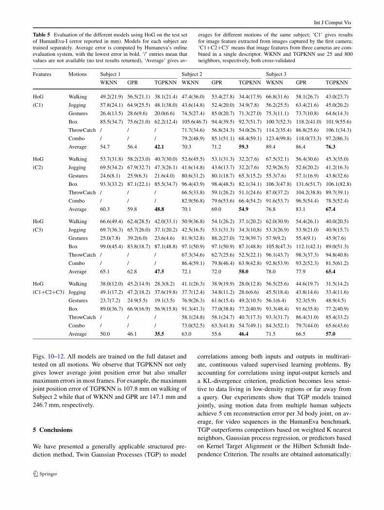
Table 5 Evaluation of the different models using HoG on the test setof HumanEva-I (error reported in mm). Models for each subject aretrained separately. Average error is computed by Humaneva’s onlineevaluation system, with the lowest error in bold. ‘/’ entries mean thatvalues are not available (no test results returned), ‘Average’ gives av-
erages for different motions of the same subject; ‘C1’ gives resultsfor image feature extracted from images captured by the first camera;‘C1+C2+C3’ means that image features from three cameras are com-bined in a single descriptor. WKNN and TGPKNN use 25 and 800neighbors, respectively, both cross-validated
Features Motions Subject 1 Subject 2 Subject 3
WKNN GPR TGPKNN WKNN GPR TGPKNN WKNN GPR TGPKNN
HoG Walking 49.2(21.9) 56.5(21.1) 38.1(21.4) 47.4(36.0) 53.4(27.8) 34.4(17.9) 66.8(31.6) 58.1(26.7) 43.0(23.7)
(C1) Jogging 57.8(24.1) 64.9(25.5) 48.1(38.0) 43.6(14.8) 52.4(20.0) 34.9(7.8) 56.2(25.5) 63.4(21.6) 45.0(20.2)
Gestures 26.4(13.5) 28.6(9.6) 20.0(6.6) 74.5(27.4) 85.0(20.7) 71.3(27.0) 75.3(11.1) 73.7(10.8) 64.6(14.3)
Box 85.5(34.7) 75.6(21.0) 62.2(12.4) 105.6(46.7) 94.4(39.5) 92.7(51.7) 100.7(52.3) 118.2(41.0) 101.9(55.6)
ThrowCatch / / / 71.7(34.6) 56.8(24.3) 54.0(26.7) 114.2(35.4) 86.8(25.6) 106.1(34.3)
Combo / / / 79.2(48.9) 85.1(51.1) 68.4(59.1) 123.4(99.8) 118.0(73.3) 97.2(86.3)
Average 54.7 56.4 42.1 70.3 71.2 59.3 89.4 86.4 76.3
HoG Walking 53.7(31.8) 58.2(23.0) 40.7(30.0) 52.6(45.5) 53.1(31.3) 32.2(7.6) 67.5(32.1) 56.4(30.6) 45.3(35.0)
(C2) Jogging 69.5(34.2) 67.9(32.7) 47.3(26.1) 41.6(14.8) 43.6(13.7) 32.2(7.6) 52.9(26.5) 52.6(20.2) 41.2(16.3)
Gestures 24.6(8.1) 25.9(6.3) 21.6(4.0) 80.6(31.2) 80.1(18.7) 65.3(15.2) 55.3(7.6) 57.1(16.9) 43.8(32.6)
Box 93.3(33.2) 87.1(22.1) 85.5(34.7) 96.4(43.9) 98.4(48.5) 82.1(34.1) 106.3(47.8) 131.6(51.7) 106.1(82.8)
ThrowCatch / / / 66.5(33.8) 59.1(26.2) 51.1(24.6) 87.0(37.2) 104.2(38.8) 89.7(39.1)
Combo / / / 82.9(56.8) 79.6(53.6) 66.4(54.2) 91.6(53.7) 96.5(54.4) 78.5(52.4)
Average 60.3 59.8 48.8 70.1 69.0 54.9 76.8 83.1 67.4
HoG Walking 66.6(49.4) 62.4(28.5) 42.0(33.1) 50.9(36.8) 54.1(26.2) 37.1(20.2) 62.0(30.9) 54.4(26.1) 40.0(20.5)
(C3) Jogging 69.7(36.3) 65.7(26.0) 37.1(20.2) 42.5(16.5) 53.1(31.3) 34.3(10,8) 53.3(26.9) 53.9(21.0) 40.9(15.7)
Gestures 25.0(7.8) 39.2(6.0) 23.6(4.6) 81.9(32.8) 88.2(27.0) 72.9(39.7) 57.9(9.2) 55.4(9.1) 45.9(7.6)
Box 99.0(45.4) 83.8(18.7) 87.1(48.8) 97.1(50.9) 97.1(50.9) 87.1(48.8) 105.8(47.3) 112.1(42.1) 89.0(51.3)
ThrowCatch / / / 67.3(34.6) 62.7(25.6) 52.5(22.1) 96.1(43.7) 98.3(37.3) 94.8(40.8)
Combo / / / 86.4(59.1) 79.8(46.4) 63.9(42.8) 92.8(53.9) 93.2(52.3) 81.5(61.2)
Average 65.1 62.8 47.5 72.1 72.0 58.0 78.0 77.9 65.4
HoG Walking 38.0(12.0) 45.2(14.9) 28.3(8.2) 41.1(26.3) 38.9(19.9) 28.0(12.8) 56.5(25.6) 44.6(19.7) 31.5(14.2)
(C1+C2+C3) Jogging 49.1(17.2) 47.2(18.2) 37.6(19.8) 37.7(12.4) 34.8(11.2) 28.6(6.6) 45.5(18.4) 43.8(14.6) 33.4(11.6)
Gestures 23.7(7.2) 24.9(5.5) 19.1(3.5) 76.9(26.3) 61.6(15.4) 49.2(10.5) 56.1(6.4) 52.3(5.9) 48.9(4.5)
Box 89.0(36.7) 66.9(16.9) 56.9(15.8) 91.3(41.3) 77.0(38.8) 77.2(40.9) 93.3(48.4) 91.6(35.8) 77.2(40.9)
ThrowCatch / / / 58.1(24.8) 58.1(24.7) 40.7(17.3) 93.3(31.7) 86.4(31.0) 85.4(33.2)
Combo / / / 73.0(52.5) 63.3(41.8) 54.7(49.1) 84.3(52.1) 79.7(44.0) 65.6(43.6)
Average 50.0 46.1 35.5 63.0 55.6 46.4 71.5 66.5 57.0
Figs. 10–12. All models are trained on the full dataset andtested on all motions. We observe that TGPKNN not onlygives lower average joint position error but also smallermaximum errors in most frames. For example, the maximumjoint position error of TGPKNN is 107.8 mm on walking ofSubject 2 while that of WKNN and GPR are 147.1 mm and246.7 mm, respectively.
5 Conclusions
We have presented a generally applicable structured pre-diction method, Twin Gaussian Processes (TGP) to model
correlations among both inputs and outputs in multivari-ate, continuous valued supervised learning problems. Byaccounting for correlations using input-output kernels anda KL-divergence criterion, prediction becomes less sensi-tive to data living in low-density regions or far away froma query. Our experiments show that TGP models trainedjointly, using motion data from multiple human subjectsachieve 5 cm reconstruction error per 3d body joint, on av-erage, for video sequences in the HumanEva benchmark.TGP outperforms competitors based on weighted K nearestneighbors, Gaussian process regression, or predictors basedon Kernel Target Alignment or the Hilbert Schmidt Inde-pendence Criterion. The results are obtained automatically:
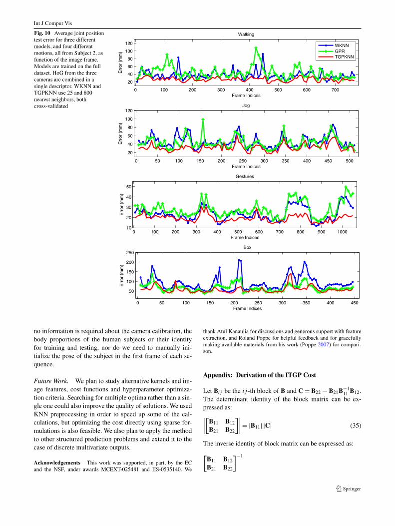
Int J Comput Vis
Fig. 10 Average joint positiontest error for three differentmodels, and four differentmotions, all from Subject 2, asfunction of the image frame.Models are trained on the fulldataset. HoG from the threecameras are combined in asingle descriptor. WKNN andTGPKNN use 25 and 800nearest neighbors, bothcross-validated
no information is required about the camera calibration, thebody proportions of the human subjects or their identityfor training and testing, nor do we need to manually ini-tialize the pose of the subject in the first frame of each se-quence.
Future Work. We plan to study alternative kernels and im-age features, cost functions and hyperparameter optimiza-tion criteria. Searching for multiple optima rather than a sin-gle one could also improve the quality of solutions. We usedKNN preprocessing in order to speed up some of the cal-culations, but optimizing the cost directly using sparse for-mulations is also feasible. We also plan to apply the methodto other structured prediction problems and extend it to thecase of discrete multivariate outputs.
Acknowledgements This work was supported, in part, by the ECand the NSF, under awards MCEXT-025481 and IIS-0535140. We
thank Atul Kanaujia for discussions and generous support with featureextraction, and Roland Poppe for helpful feedback and for gracefullymaking available materials from his work (Poppe 2007) for compari-son.
Appendix: Derivation of the ITGP Cost
Let Bij be the ij -th block of B and C = B22 − B21B−111 B12.
The determinant identity of the block matrix can be ex-pressed as:∣∣∣∣
[B11 B12
B21 B22
]∣∣∣∣= |B11| |C| (35)
The inverse identity of block matrix can be expressed as:
[B11 B12
B21 B22
]−1
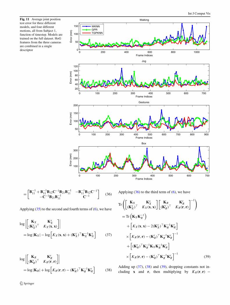
Int J Comput Vis
Fig. 11 Average joint positiontest error for three differentmodels, and four differentmotions, all from Subject 1,function of timestep. Models aretrained on the full dataset. HoGfeatures from the three camerasare combined in a singledescriptor
=[
B−111 + B−1
11 B12C−1B21B−111 −B−1
11 B12C−1
−C−1B21B−111 C−1
](36)
Applying (35) to the second and fourth terms of (6), we have
log
∣∣∣∣
[KX Kx
X
(KxX)� KX(x,x)
]∣∣∣∣
= log |KX| − log[KX(x,x) + (Kx
X)�K−1X Kx
X
](37)
log
∣∣∣∣
[KR Kr
R
(KrR)� KR(r, r)
]∣∣∣∣
= log |KR| + log[KR(r, r) − (Kr
R)�K−1R Kr
R
](38)
Applying (36) to the third term of (6), we have
Tr
([KX Kx
X
(KxX)� KX(x,x)
][KR Kr
R
(KrR)� KR(r, r)
]−1)
= Tr(
KXK−1R
)
+[KX(x,x) − 2(Kx
X)�K−1R Kr
R
]
×[KR(r, r) − (Kr
R)�K−1R Kr
R
]−1
+[(Kr
R)�K−1R KXK−1
R KrR
]
×[KR(r, r) − (Kr
R)�K−1R Kr
R
]−1(39)
Adding up (37), (38) and (39), dropping constants not in-cluding x and r, then multiplying by KR(r, r) −
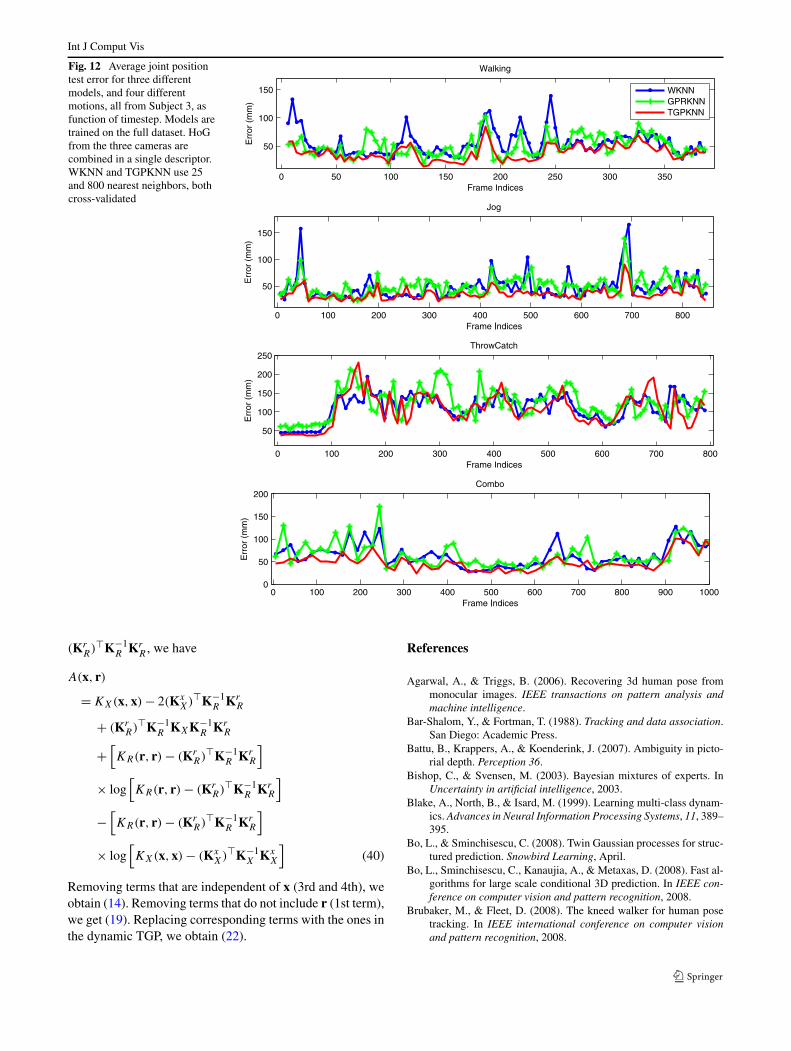
Int J Comput Vis
Fig. 12 Average joint positiontest error for three differentmodels, and four differentmotions, all from Subject 3, asfunction of timestep. Models aretrained on the full dataset. HoGfrom the three cameras arecombined in a single descriptor.WKNN and TGPKNN use 25and 800 nearest neighbors, bothcross-validated
(KrR)�K−1
R KrR , we have
A(x, r)
= KX(x,x) − 2(KxX)�K−1
R KrR
+ (KrR)�K−1
R KXK−1R Kr
R
+[KR(r, r) − (Kr
R)�K−1R Kr
R
]
× log[KR(r, r) − (Kr
R)�K−1R Kr
R
]
−[KR(r, r) − (Kr
R)�K−1R Kr
R
]
× log[KX(x,x) − (Kx
X)�K−1X Kx
X
](40)
Removing terms that are independent of x (3rd and 4th), weobtain (14). Removing terms that do not include r (1st term),we get (19). Replacing corresponding terms with the ones inthe dynamic TGP, we obtain (22).
References
Agarwal, A., & Triggs, B. (2006). Recovering 3d human pose frommonocular images. IEEE transactions on pattern analysis andmachine intelligence.
Bar-Shalom, Y., & Fortman, T. (1988). Tracking and data association.San Diego: Academic Press.
Battu, B., Krappers, A., & Koenderink, J. (2007). Ambiguity in picto-rial depth. Perception 36.
Bishop, C., & Svensen, M. (2003). Bayesian mixtures of experts. InUncertainty in artificial intelligence, 2003.
Blake, A., North, B., & Isard, M. (1999). Learning multi-class dynam-ics. Advances in Neural Information Processing Systems, 11, 389–395.
Bo, L., & Sminchisescu, C. (2008). Twin Gaussian processes for struc-tured prediction. Snowbird Learning, April.
Bo, L., Sminchisescu, C., Kanaujia, A., & Metaxas, D. (2008). Fast al-gorithms for large scale conditional 3D prediction. In IEEE con-ference on computer vision and pattern recognition, 2008.
Brubaker, M., & Fleet, D. (2008). The kneed walker for human posetracking. In IEEE international conference on computer visionand pattern recognition, 2008.
Int J Comput Vis
Choo, K., & Fleet, D. (2001). People tracking using hybrid MonteCarlo filtering. In IEEE international conference on computer vi-sion, 2001.
CMU (2003). Human Motion DataBase. Online at http://mocap.cs.cmu.edu/search.html.
Cortes, C., Mohri, M., & Weston, J. (2005). A general regression tech-nique for learning transductions. In International conference onmachine learning (pp. 153–160) 2005.
Cristianini, N., Shawe-Taylor, J., Elisseeff, A., & Kandola, J. S.(2001a). On kernel-target alignment. In Advances in neural in-formation processing systems (pp. 367–373) 2001.
Cristianini, N., Shawe-Taylor, J., & Kandola, J. S. (2001b). Spectralkernel methods for clustering. In Advances in neural informationprocessing systems (pp. 649–655) 2001.
Dalal, N., & Triggs, B. (2005). Histograms of oriented gradients forhuman detection. In IEEE international conference on computervision and pattern recognition, 2005.
Deutscher, J., Blake, A., & Reid, I. (2000). Articulated body motioncapture by annealed particle filtering. In IEEE international con-ference on computer vision and pattern recognition, 2000.
Deutscher, J., Davidson, A., & Reid, I. (2001). Articulated partition-ing of high dimensional search spaces associated with articulatedbody motion capture. In IEEE international conference on com-puter vision and pattern recognition, 2001.
Duane, S., Kennedy, A. D., Pendleton, B. J., & Roweth, D. (1987).Hybrid Monte Carlo. Physics Letters B, 195(2), 216–222.
Elgammal, A., & Lee, C. (2004). Inferring 3d body pose from silhou-ettes using activity manifold learning. In IEEE international con-ference on computer vision and pattern recognition, 2004.
Geurts, P., Wehenkel, L., & d’Alché Buc, F. (2006). Kernelizing theoutput of tree-based methods. In International conference on ma-chine learning (pp. 345–352) 2006.
Geurts, P., Wehenkel, L., & d’Alché Buc, F. (2007). Gradient boost-ing for kernelized output spaces. In International conference onmachine learning, New York, NY, USA (pp. 289–296) 2007.
Gretton, A., Bousquet, O., Smola, A. J., & Schölkopf, B. (2005a).Measuring statistical dependence with Hilbert-Schmidt norms. InS. Jain & W.-S. Lee (Eds.), Proceedings algorithmic learning the-ory, 2005.
Gretton, A., Herbrich, R., Smola, A. J., Bousquet, O., & Schölkopf, B.(2005b). Kernel methods for measuring independence. Journal ofMachine Learning Research, 6, 2075–2129.
Guzman, A. N., & Holden, S. (2007). Twinned Gaussian processes.In Advances in neural information processing systems, December2007.
Hinton, G. E., & Roweis, S. T. (2002). Stochastic neighbor embedding.In Advances in neural information processing systems (pp. 833–840) 2002.
Isard, M., & Blake, A. (1998). CONDENSATION—conditional den-sity propagation for visual tracking. International Journal ofComputer Vision.
Kanaujia, A., Sminchisescu, C., & Metaxas, D. (2006). Semi-supervised hierarchical models for 3D human pose reconstruc-tion. In IEEE international conference on computer vision andpattern recognition, 2006.
Kanaujia, A., Sminchisescu, C., & Metaxas, D. (2007). Spectral latentvariable models for perceptual inference. In IEEE InternationalConference on Computer Vision, Vol. 1, 2007.
Kehl, R., Bray, M., & Gool, L. V. (2005). Full body tracking frommultiple views using stochastic sampling. In IEEE internationalconference on computer vision and pattern recognition, 2005.
Koenderink, J. (1998). Pictorial relief. Philosophical TransactionsRoyal Society London A 356.
Koenderink, J., & van Doorn, A. (1979). The internal representation ofsolid shape with respect to vision. Biological Cybernetics 32(3).
Krauthgamer, R., & Lee, J. R. (2004). Navigating nets: simple algo-rithms for proximity search. In SODA ’04: Proceedings of the fif-teenth annual ACM-SIAM symposium on discrete algorithms (pp.798–807) 2004.
Lafferty, J., McCallum, A., & Pereira, F. (2001). Conditional randomfields: probabilistic models for segmenting and labeling sequencedata. In International conference on machine learning, 2001.
Lawrence, N. (2005). Probabilistic non-linear component analysis withGaussian process latent variable models. Journal of MachineLearning Research, 6, 1783–1816.
Lee, H. J., & Chen, Z. (1985). Determination of 3D human body pos-tures from a single view. Computer Vision, Graphics and ImageProcessing, 30, 148–168.
Li, R., Yang, M., Sclaroff, S., & Tian, T. (2006). Monocular tracking of3D human motion with a coordinated mixture of factor analyzers.In European conference on computer vision, 2006.
Lowe, D. (2004). Distinctive image features from scale-invariant key-points. International Journal of Computer Vision, 60(2).
Memisevic, R. (2006). Kernel information embeddings. In Interna-tional conference on machine learning, 2006.
Morris, D., & Rehg, J. (1998). Singularity analysis for articulated ob-ject tracking. In IEEE international conference on computer vi-sion and pattern recognition (pp. 289–296) 1998.
Neal, R. (1998). Annealed importance sampling (Technical Report9805). Department of Statistics, University of Toronto.
Poppe, R. (2007). Evaluating example-based human pose estimation:Experiments on HumanEva sets. In HumanEva Workshop CVPR,2007.
Rasmussen, C. E., & Williams, C. K. I. (2006). Gaussian processes formachine learning. Adaptive computation and machine learning.Cambridge: MIT Press.
Rosales, R., & Sclaroff, S. (2002). Learning body pose via special-ized maps. In Advances in neural information processing systems,2002.
Roth, S., Sigal, L., & Black, M. (2004). Gibbs likelihoods for Bayesiantracking. In IEEE international conference on computer visionand pattern recognition, 2004.
Schaal, S., Atkeson, C., & Moore, A. (1997). Locally weighted learn-ing. Artificial Intelligence Review, 11, 11–73.
Serre, T., Wolf, L., Bileschi, S., & Riesenhuber, M. (2007). Robust ob-ject recognition with cortex-like mechanisms. IEEE Transactionson Pattern Analysis and Machine Intelligence, 29(3), 411–426.
Shakhnarovich, G., Viola, P., & Darrell, T. (2003). Fast pose estimationwith parameter sensitive hashing. In IEEE international confer-ence on computer vision, 2003.
Sidenbladh, H., & Black, M. (2001). Learning image statistics forBayesian tracking. In IEEE international conference on computervision, 2001.
Sidenbladh, H., Black, M., & Fleet, D. (2000). Stochastic tracking of3D human figures using 2D image motion. In European confer-ence on computer vision, 2000.
Sidenbladh, H., Black, M., & Sigal, L. (2002). Implicit probabilisticmodels of human motion for synthesis and tracking. In Europeanconference on computer vision, 2002.
Sigal, L., & Black, M. (2006). HumanEva: synchronized video and mo-tion capture dataset for evaluation of articulated human motion(Technical Report CS-06-08). Brown University.
Sigal, L., Balan, A., & Black, M. J. (2007). Combined discriminativeand generative articulated pose and non-rigid shape estimation. InAdvances in neural information processing systems, 2007.
Sminchisescu, C. (2002). Consistency and coupling in human modellikelihoods. In IEEE international conference on automatic faceand gesture recognition (pp. 27–32). Washington, DC, 2002.
Sminchisescu, C., & Jepson, A. (2004a). Generative modeling for con-tinuous non-linearly embedded visual inference. In Internationalconference on machine learning (pp. 759–766). Banff, 2004.
Int J Comput Vis
Sminchisescu, C., & Jepson, A. (2004b). Variational mixture smooth-ing for non-linear dynamical systems. In IEEE international con-ference on computer vision and pattern recognition (Vol. 2, pp.608–615). Washington, DC, 2004.
Sminchisescu, C., & Telea, A. (2002). Human pose estimation fromsilhouettes. A consistent approach using distance level sets. InWSCG international conference for computer graphics, visualiza-tion and computer vision, Czech Republic, 2002.
Sminchisescu, C., & Triggs, B. (2001). Covariance-scaled sampling formonocular 3D body tracking. In IEEE international conferenceon computer vision and pattern recognition (Vol. 1, pp. 447–454).Hawaii, 2001.
Sminchisescu, C., & Triggs, B. (2002a). Building roadmaps of localminima of visual models. In European conference on computervision (Vol. 1, pp. 566–582). Copenhagen, 2002.
Sminchisescu, C., & Triggs, B. (2002b). Hyperdynamics importancesampling. In European conference on computer vision (Vol. 1, pp.769–783). Copenhagen, 2002.
Sminchisescu, C., & Triggs, B. (2003). Kinematic jump processes formonocular 3D human tracking. In IEEE international conferenceon computer vision and pattern recognition (Vol. 1, pp. 69–76).Madison, 2003.
Sminchisescu, C., & Triggs, B. (2005). Mapping minima and transi-tions in visual models. International Journal of Computer Vision61(1).
Sminchisescu, C., & Welling, M. (2007). Generalized darting Monte-Carlo. In Artificial Intelligence and Statistics, Vol. 1, 2007.
Sminchisescu, C., Kanaujia, A., Li, Z., & Metaxas, D. (2005). Condi-tional visual tracking in kernel space. In Advances in neural in-formation processing systems, 2005.
Sminchisescu, C., Kanaujia, A., & Metaxas, D. (2006). Learning jointtop-down and bottom-up processes for 3D visual inference. In
IEEE international conference on computer vision and patternrecognition, 2006.
Sminchisescu, C., Kanaujia, A., & Metaxas, D. (2007). BM3E: dis-criminative density propagation for visual tracking. IEEE Trans-actions on Pattern Analysis and Machine Intelligence.
Smola, A. J., & Schölkopf, B. (2000). Sparse greedy matrix approxi-mation for machine learning. In International conference on ma-chine learning (pp. 911–918) 2000.
Taskar, B., Guestrin, C., & Koller, D. (2004). Max-margin Markovnetworks. In Advances in neural information processing systems,2004.
Tresp, V. (2000). Mixtures of Gaussian processes. In Advances inneural information processing systems, 2000.
Tsochantaridis, I., Hofmann, T., Joachims, T., & Altun, Y. (2004). Sup-port vector machine learning for interdependent and structuredoutput spaces. In International conference on machine learning,2004.
Urtasun, R., Fleet, D., Hertzmann, A., & Fua, P. (2005). Priors for peo-ple tracking in small training sets. In IEEE international confer-ence on computer vision, 2005.
Vincent, P., & Bengio, Y. (2002). Kernel matching pursuit. MachineLearning, 48, 165–187.
Vondrak, M., Sigal, L., & Jenkins, O. C. (2008). Physical simulation forprobabilistic motion tracking. In IEEE international conferenceon computer vision and pattern recognition, 2008.
Wang, J., Fleet, D. J., & Hertzmann, A. (2008). Gaussian process dy-namical models. In IEEE transactions on pattern analysis andmachine intelligence, 2008.
Weston, J., Chapelle, O., Elisseeff, A., Scholkopf, B., & Vapnik, V.(2002). Kernel dependency estimation. In Advances in neural in-formation processing systems, 2002.