Tutorial on Operating Characteristics of Microprocessor-Based Multiterminal Line

Current Differential Relays

Bogdan Kasztenny, Gabriel Benmouyal, Héctor J. Altuve, and Normann Fischer Schweitzer Engineering Laboratories, Inc.

Published in Line Current Differential Protection: A Collection of

Technical Papers Representing Modern Solutions, 2014

Previously presented at the 66th Annual Georgia Tech Protective Relaying Conference, April 2012

Previous revised edition released November 2011

Originally presented at the 38th Annual Western Protective Relay Conference, October 2011

1

Tutorial on Operating Characteristics of Microprocessor-Based Multiterminal Line

Current Differential Relays Bogdan Kasztenny, Gabriel Benmouyal, Héctor J. Altuve, and Normann Fischer,

Schweitzer Engineering Laboratories, Inc.

Abstract—Line current differential (87L) protection schemes face extra challenges compared with other forms of differential protection, in addition to the traditional requirements of sensitivity, speed, and immunity to current transformer saturation. Some of these challenges include data communication, alignment, and security; line charging current; and limited communications bandwidth.

To address these challenges, microprocessor-based 87L relays apply elaborate operating characteristics, which are often different than a traditional percentage differential characteristic used for bus or transformer protection. These sophisticated elements may include adaptive restraining terms, apply an Alpha Plane, use external fault detection logic for extra security, and so on.

While these operating characteristics provide for better performance, they create the following challenges for users:

• Understanding how the 87L elements make the trip decision.

• Understanding the impact of 87L settings on sensitivity and security, as well as grasping the relationship between the traditional percentage differential characteristic and the various 87L operating characteristics.

• Having the ability to transfer settings between different 87L operating characteristics while keeping a similar balance between security and dependability.

• Testing the 87L operating characteristics. These issues become particularly significant in applications

involving more than two currents in the line protection zone (multiterminal lines) and lines terminated on dual-breaker buses.

This paper is a tutorial on this relatively new protection topic and offers answers to the outlined challenges.

I. INTRODUCTION The current differential principle is the most powerful

short-circuit protection method. Responding to all currents bounding the zone of protection, the principle has a very high potential for both sensitivity (effectively, it sees the fault current at the place of an internal fault) and security (effectively, it sees an external fault current flowing in and out of the protection zone). Also, differential protection is typically easy to apply because it does not require elaborate short-circuit studies and settings calculations.

In its application to power lines, the principle is little or not affected by weak terminals, series compensation, changing short-circuit levels, current inversion, power swings, nonstandard short-circuit current sources, and many other

issues relevant for protection techniques based on measurements from a single line terminal [1].

Differential protection applied to buses, transformers, generators, or motors is well-researched and belongs to a mature field of protective relaying. In contrast, microprocessor-based 87L schemes began to be commonly applied less than 15 years ago and belong to a relatively new field with only the second generation of relays available in the market.

Each type of differential protection faces its own unique challenges. Transformer differential protection must deal with fictitious differential signals caused by magnetizing inrush conditions while striving for fast operation and sensitivity to turn-to-turn faults, for example. Line current differential protection is no exception. Its challenges include the requirement of high sensitivity, current alignment issues, security under current transformer (CT) saturation, line charging current, limited bandwidth channels, channel impairments, and failure modes, to mention the key challenges.

Present 87L elements are sophisticated and adaptive in order to maintain the simplicity of application inherent in the differential principle itself, while addressing challenges related to applications to power lines.

This paper is a tutorial on the operating characteristics of 87L elements. We focus on practical implementations actually available in present 87L relays.

We start with an overview of challenges inherent in 87L applications and then review the two main implementations in great detail—the percentage differential and the Alpha Plane differential elements. We highlight their similarities and differences as well as relative strengths. Other operating principles exist, but they are either theoretical or not commonly used and are not covered in this paper.

We follow with a description of a generalized Alpha Plane principle that merges the two-restraint Alpha Plane and multiterminal percentage differential approaches, allowing us to benefit from the relative strengths of each.

Next, we focus on solutions to three challenges of 87L protection: security under external faults and CT saturation, security under current alignment errors, and line charging currents.

2

Finally, we discuss the high adaptivity of 87L elements, which results from addressing the challenges, and the impact of that adaptivity on settings selection and testing.

This tutorial provides in-depth coverage of the topic with specific equations and numerical examples using steady-state values, as well as waveforms from transient simulation studies.

We assume the reader has a background in differential protection in general, as well as in line protection requirements and general principles. We also assume the reader has basic knowledge of signal processing methods used in microprocessor-based relays, such as Fourier or cosine filtering. The references provide the required background knowledge and allow for further reading to explore some of the topics in greater detail.

The goal of this paper is to contribute to the better understanding of microprocessor-based 87L relays and bring appreciation to the advancements achieved by relay designers and application engineers over the last decade.

II. CHALLENGES OF LINE CURRENT DIFFERENTIAL PROTECTION

Line current differential applications create several new challenges in addition to the general considerations applicable to bus, transformer, generator, and other forms of differential protection. These challenges stem from the fact that a power line is not a contained piece of apparatus, like a bus or a power transformer, but stretches across a distance. The following subsections elaborate on specific issues resulting from the size of lines as protected elements.

A. Sensitivity Requirements Short circuits on power lines can happen under a variety of

conditions, including high soil resistivity increasing the tower grounding resistance, contact with trees and other objects, isolator flashover due to contamination, ionization of air due to fires in the vegetation along the right of way, and impact of wind, to name the most common factors.

Grounding of power line towers is less effective than substation grounding, and power lines are not surrounded with many solidly grounded objects. As a result, short circuits on power lines can be accompanied by relatively high fault resistance, particularly for single-line-to-ground faults.

High-resistance line faults draw limited currents and do not normally impact the power system from the dynamic stability and equipment damage points of view. However, power lines are located in public space, and as such, short circuits on power lines can contribute to secondary effects (such as human safety issues and property damage) if not detected with adequate sensitivity and speed.

Therefore, the sensitivity of 87L protection is an important consideration.

B. Line Charging Current Long transmission lines and cables can draw a substantial

amount of charging current. The line charging current is not measured by the 87L scheme as an input and therefore appears as a fictitious differential signal, jeopardizing security.

Line energization is the most demanding scenario when considering the line charging current.

First, the charging current is supplied through the single circuit breaker that just energized the line, and therefore, the charging current appears as a single-end feed. No restraining action is possible because there is no other current to use for restraining. Elevating the 87L element pickup, the classical solution to maintain security, reduces sensitivity.

Second, the line energization current has a transient inrush component in it, with peak values much higher than the steady-state charging current, calling for even higher pickup thresholds, at least temporarily until the capacitive inrush current subsides.

During symmetrical conditions, the line charging current is a positive-sequence current. This allows 87L elements that respond to negative- and/or zero-sequence differential signals to mitigate problems related to the line charging current. However, under unbalanced conditions, negative- or zero-sequence charging currents may appear in response to negative- or zero-sequence voltages. Good examples to consider are breaker pole scatter during line energization or external faults in very weak systems causing line voltage unbalance and making the line draw sequence charging currents.

C. Series-Compensated Lines Series-compensated lines create unique protection

problems due to the capacitive reactance included in series with the protected line, potentially causing voltage and current inversion [1] [2]. In addition, the capacitor overvoltage protection makes the series capacitor circuit nonlinear, and unequal bypassing actions between the phases create series unbalance at the point of the capacitor installation. This series unbalance couples the sequence networks that represent the protected line, thus challenging traditional protection assumptions and relationships between sequence currents and voltages during both internal and external faults.

It is common knowledge that the differential principle is not affected by series compensation. This is only partially correct. Of course, the principle is not jeopardized from the security point of view, but current inversion and coupling between sequence networks create challenges from the dependability point of view. Series compensation may also delay 87L operation for internal faults [1] [3].

D. Communications Channel Because lines span long distances, it is better to think of

87L protection as 87L schemes, rather than 87L relays. The 87L schemes comprise two or more relays that need to share their local currents measured in different substations located miles or even hundreds of miles apart. These separate relays therefore require a channel for exchanging current values as a part of the 87L scheme. In this respect, both analog and microprocessor-based implementations face considerable challenges, even though specific problems are different for the analog and microprocessor-based schemes.

Analog schemes using pilot wires can only be applied to very short lines because of signal attenuation due to the series

3

resistance and shunt capacitance of the pilot wires. In order to reduce the number of pilot wires, these schemes often combine the phase currents into one signal instead of using the phase-segregated approach.

Microprocessor-based relays utilize long-haul digital communications to exchange the current signals, thus avoiding the limitation of the line length.

However, the following new challenges arise in microprocessor-based implementations:

• Because they work on digital data derived from current samples, these implementations require the means to align the local and remote current measurements so that currents taken at the same time are used in the differential calculations (see Section II, Subsection E).

• Long-haul channels, unless they use direct fiber, are often built with general purpose communications equipment. These networks are prone to various impairments that create both security and dependability problems for 87L schemes (see Section II, Subsection F).

• The available bandwidth (i.e., the amount of data that can be shared within any period of time) is limited, at least historically (see Section II, Subsection G).

E. Alignment of Digital Current Values Microprocessor-based relays using the differential principle

need current data to have the same time reference. In bus, transformer, or generator protection, this is accomplished naturally by using a single protective device that directly receives all the required currents and samples them in a synchronized fashion. Microprocessor-based 87L schemes need an explicit method to synchronize or align the currents taken by separate 87L relays at various line terminals.

When using symmetrical channels (equal latencies in the transmitting and receiving directions), 87L schemes can align the data using the industry standard method known as the ping-pong algorithm. When the channel is not symmetrical, the ping-pong algorithm fails, yielding a current phase error proportional to the amount of asymmetry, which, in turn, creates a fictitious differential signal.

One solution is to use a common time reference to drive the current sampling (historically, Global Positioning System [GPS] clocks). However, reliance on GPS and associated devices for protection is not a commonly accepted solution.

In addition, channel latency may change in response to communications path switching when using multiplexed channels. This problem calls for proper data handling methods built in the 87L relays. In general, each relay needs to wait for the slowest channel to deliver the remote current data, but at the same time, the alignment delay needs to be as short as possible in order not to penalize the speed of operation.

F. Channel Impairments Bit errors, asymmetry, unintentional cross-connections

between separate 87L schemes, path switching, accidental loopbacks, and frame slips are examples of impairments, or

events in the long-haul communications network that may affect performance of 87L schemes.

Specific solutions are applied to each of these problems, such as disturbance detection supervision for undetected bit errors or relay addressing for unintended cross-connections and loopbacks [4]. Still, it is beneficial for the 87L operating characteristic itself to have a ride-through ability to prevent or mitigate the impact of channel impairments.

G. Channel Bandwidth Limitation Historically, microprocessor-based 87L schemes are

required to work with 56 kbps or 64 kbps channels originally created by the telecommunications industry to carry voice data. A 64 kbps channel allows the clocking of about 260 bits of data in a quarter of a power cycle. Given the necessary overhead, such as packet framing, data integrity protection, and relay addressing, the room left to send current data is very limited, much lower than 260 bits every quarter of a power cycle. By comparison, bus, transformer, or generator differential relays have practically unlimited access (in terms of analog-to-digital converter resolution and sampling frequency) to all the protection zone boundary currents.

The channel bandwidth restriction is an important consideration because it limits the visibility of the local relay into the situation at the remote terminals. For example, in dual-breaker applications, the local relay ideally measures both breaker currents individually at the remote substation, but sending both current measurements doubles the packet payload.

The limited channel bandwidth makes the application of tried-and-true protection solutions and algorithms in 87L designs more challenging. The next subsection describes the most relevant example of this challenge.

H. CT Saturation for External Faults Because of its required sensitivity, differential protection

must include countermeasures to CT errors, saturation during external faults in particular. External fault detection algorithms are known in the art of bus or transformer protection. These algorithms detect external fault events before any CT saturation occurs and engage extra security measures to prevent relay misoperation. These measures can include an increase in the restraining action and an extra intentional time delay, among others.

However, effective external fault detection algorithms require access to all the zone boundary currents with high fidelity (samples taken at relatively high sampling rates). This requirement may be challenging in 87L applications because of the channel bandwidth limitation. As a result, simplified external fault detection algorithms are often used, or the 87L operating characteristic is designed for better immunity to CT saturation at some expense of sensitivity.

I. Phase and Sequence Differential Elements Phase differential (87LP) elements face two challenges in

87L applications. First, because they add the currents to create a differential signal, these elements are prone to misoperation for external faults if the currents were misaligned, such as

4

when using asymmetrical channels in the ping-pong synchronization mode. Second, because they use the through currents (load or external fault currents) for restraining, these elements have limited sensitivity, despite the fact that their differential signals are not impacted by load. Setting the phase differential elements to be more sensitive only increases the danger of misoperation due to channel asymmetry, and the issues of immunity to alignment errors and sensitivity cannot be easily reconciled in phase differential element applications.

This observation inspired sequence differential elements—single-phase elements responding to the negative- or zero-sequence differential current (87LQ and 87LG, respectively) and stabilized with the corresponding sequence through current. This way, the load component is removed not only from the differential signal but also from the restraining action, thus allowing for much higher sensitivity. At the same time, the standing sequence currents are very low (ideally zero) during normal system operation, which mitigates the effect of temporary current misalignment, such as that due to asymmetrical channels.

In addition, sequence networks are typically very homogeneous, which keeps the relative angles of the sequence currents of the line protection zone almost perfectly in phase for internal faults. This fact provides a good margin when balancing protection dependability and security. Relative immunity to line charging current is yet another advantage of sequence differential elements.

However, the high sensitivity of sequence differential elements makes them prone to misoperate on external faults accompanied with CT errors. Consider a three-phase balanced fault, such as when closing on safety grounds inadvertently left after equipment maintenance. True (primary) negative- and zero-sequence currents equal zero (or are very close to zero), but saturation of one or more CTs would generate fictitious negative- or zero-sequence components in the secondary currents. A negative- or zero-sequence differential scheme would experience security issues due to the fictitious differential signal. Restraining is very difficult because one of the line terminals would measure a fictitious non-zero sequence current, while the other terminals may correctly measure a zero value in the sequence current. A sequence differential scheme would not have any actual through negative- and zero-sequence current for restraining. Similar concerns apply to the zero-sequence current measurements during faults not involving ground.

These considerations make the external fault detection algorithms and channel bandwidth limitations even more relevant.

The challenges related to microprocessor-based multiterminal 87L protection described so far call for a multidimensional optimization of the relay design, involving protection algorithms, signal processing, communications issues, and so on. The 87L operating characteristic (the mapping of individual currents around the protection zone into a trip decision) plays an important role in addressing these problems. Different solutions have emerged since the introduction of microprocessor-based 87L relays.

In the remainder of this paper, we review details of some of the key solutions to the stated challenges.

III. PERCENTAGE DIFFERENTIAL CHARACTERISTIC

A. Differential Signal A differential element responds to a differential (operating)

signal. Equation (1) defines the differential signal iDIF for a line bounded by N currents, i1 through iN. DIF 1 2 Ni i i i= + + + (1)

For example, a three-terminal line connected to a breaker-and-a-half bus at each terminal is bounded by six currents per phase.

The differential signal may be used in a number of ways by the differential element, but the primary purpose is to check the level of the differential signal to qualify an internal fault. For this reason, the differential signal is typically filtered for better accuracy, and its magnitude is derived:

DIF DIFI i= (2)

where: | | denotes an operation of filtering and magnitude estimation.

Depending on the relay design and the particular processing of the differential signal in the relay algorithm, filtering and magnitude estimation can use a cosine or Fourier filter, or even absolute values of instantaneous samples. Filters may use half-cycle, full-cycle, or variable data windows. Moreover, a given relay may process the same differential signal (1) in multiple ways simultaneously, with resulting magnitudes (2) serving different parts of the differential element algorithm.

Designs that work on samples execute (1) first and follow with filtering and magnitude estimation per (2). Designs that work on phasors calculate phasors first, apply (1) to phasors, and follow with magnitude estimation per (2). The final outcome is the same, but there are significant differences between the two approaches (samples versus phasors) when it comes to the amount of data sent and amount of information available to remote relays. In general, 87L designs that work on samples are more potent because they have access to more information in the remote currents.

The phase differential (87LP) elements respond to the per-phase differential signals (1). The sequence differential (87LQ and 87LG) elements respond to the differential signal derived from the negative- or zero-sequence phasors calculated first from the phase currents. For example:

( ) 1Q 2Q NQDIF QI Ī Ī Ī= + + + (3)

B. Restraining Signal As explained in Section II, the differential signal can differ

from zero for a number of events, not only for internal faults. Many of the sources of the fictitious differential signal depend on the magnitudes of the line currents (the greater the currents, the greater the fictitious differential signal). CT errors and

5

current alignment errors are good examples of this relationship.

This observation led to the application of percentage differential elements [5]. The element develops a restraining signal and uses a portion of it (a percentage) to qualify the differential signal. Therefore, the function of the restraining signal is to reflect the overall current level for all the line currents (the through current). This function can be fulfilled in a number of ways. Unlike the differential signal, which is created in the same universal way by all differential relays, the restraining signal is an arbitrary signal and, as such, is design-dependent.

Equations (4) and (5) describe typical restraining signals, IRST, for multiterminal lines.

RST 1 2 NI i i i= + + + (4)

( )RST 1 2 NI max i , i , , i= … (5)

Most relays use one of these two expressions. Reference [6] provides more information on various ways of creating the restraining signal.

In general, the restraining signal alone can provide security only up to a certain degree of CT saturation, as we show in Section VII. As a result, advanced relays tend to rely on mechanisms other than a simple restraint during extreme CT saturation.

Combinations of the approaches (4) and (5) are possible. For example, the local currents at each terminal (in dual-breaker applications) can be treated using (4), and subsequently, the consolidated local and remote currents can be aggregated in the total restraining signal using (5).

Similar to the differential signal, the restraining signal can be processed using different filters of different window lengths or can use absolute values of instantaneous samples. Moreover, multiple restraining signals can be calculated for usage in different parts of the 87L algorithm. For example, using full-cycle cosine filtering in (2), (4), and (5) provides accurate differential and restraining signals, suitable for percentage differential characteristics. Using absolute values of samples in these operations provides faster, less accurate instantaneous differential and restraining signals, suitable for external fault detection algorithms.

The 87LP elements respond to the per-phase restraining signals. The 87LQ and 87LG elements respond to the restraining signal derived from the negative- or zero-sequence phasors calculated first from the phase currents. For example:

( ) 1Q 2Q NQRST QI Ī Ī Ī= + + + (6)

During three-phase balanced faults, the restraining signals of the 87LQ and 87LG elements are zero, and during phase-to-phase faults, the restraining signal of the 87LG element is zero. Therefore, the restraining signal defined as (6) for these elements fails to meet its primary function of providing security for the mentioned fault types, and extra security measures are needed to secure the sequence elements for these fault types.

C. Operating Characteristic A percentage differential element operates when the

differential signal is above a constant pickup value: DIFI P> (7)

and above a percentage of the restraining signal: DIF RSTI K • I> (8)

Some relays may combine numerically, rather than logically, the pickup and restraining conditions: DIF RSTI P K • I> + (9)

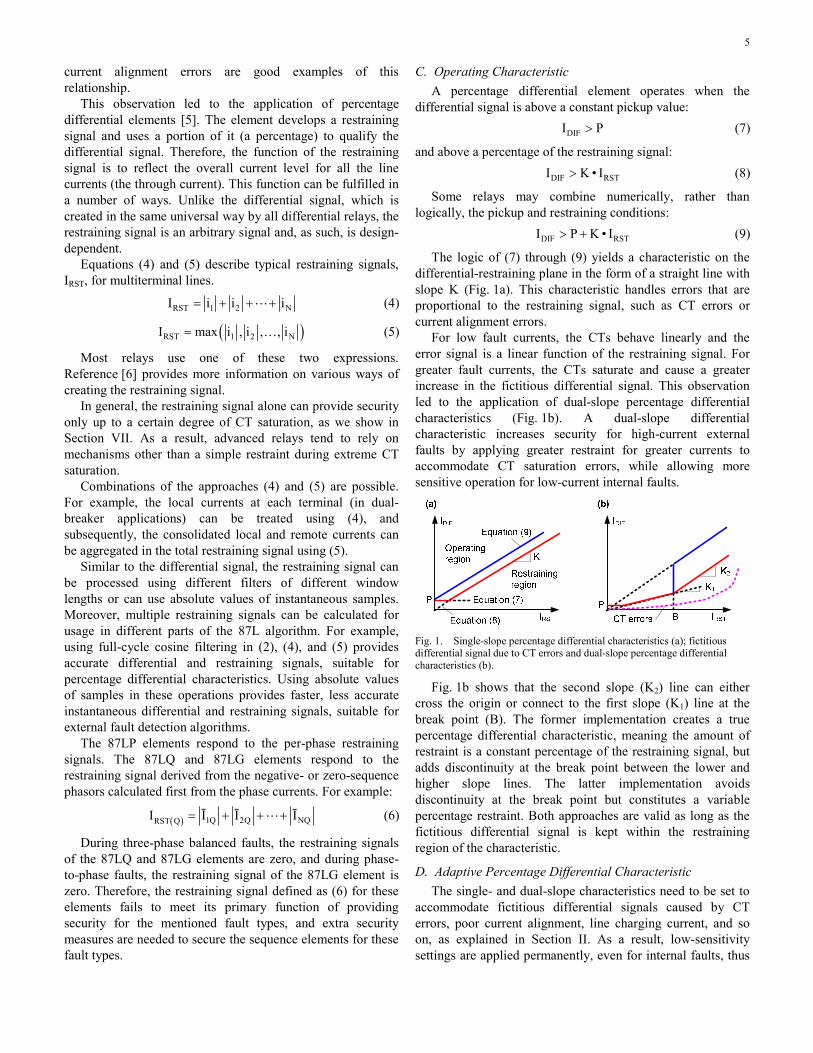
The logic of (7) through (9) yields a characteristic on the differential-restraining plane in the form of a straight line with slope K (Fig. 1a). This characteristic handles errors that are proportional to the restraining signal, such as CT errors or current alignment errors.

For low fault currents, the CTs behave linearly and the error signal is a linear function of the restraining signal. For greater fault currents, the CTs saturate and cause a greater increase in the fictitious differential signal. This observation led to the application of dual-slope percentage differential characteristics (Fig. 1b). A dual-slope differential characteristic increases security for high-current external faults by applying greater restraint for greater currents to accommodate CT saturation errors, while allowing more sensitive operation for low-current internal faults.

Fig. 1. Single-slope percentage differential characteristics (a); fictitious differential signal due to CT errors and dual-slope percentage differential characteristics (b).

Fig. 1b shows that the second slope (K2) line can either cross the origin or connect to the first slope (K1) line at the break point (B). The former implementation creates a true percentage differential characteristic, meaning the amount of restraint is a constant percentage of the restraining signal, but adds discontinuity at the break point between the lower and higher slope lines. The latter implementation avoids discontinuity at the break point but constitutes a variable percentage restraint. Both approaches are valid as long as the fictitious differential signal is kept within the restraining region of the characteristic.

D. Adaptive Percentage Differential Characteristic The single- and dual-slope characteristics need to be set to

accommodate fictitious differential signals caused by CT errors, poor current alignment, line charging current, and so on, as explained in Section II. As a result, low-sensitivity settings are applied permanently, even for internal faults, thus

6

limiting sensitivity of the 87L element or even jeopardizing its dependability.

Adaptive differential elements control the restraining action dynamically using dedicated logic to detect conditions that require more security and engage the extra security only when required. This adaptive behavior can be achieved typically in two ways.

One solution uses two sets of settings (normal and extended security) and settings switchover logic to toggle between the normal and extended security. Normal security settings, in effect most of the time, provide high sensitivity. The adaptive element switches to the less-sensitive extended security settings only when required in response to rare or abnormal events. Settings switchover may be triggered by external fault detection (Section VII), poor data alignment (Section VIII), loss of charging current compensation (Section IX), and so on.

Fig. 2 illustrates the concept of adaptive percentage restraint settings. Typically, only the percentage restraint (slope) is increased, but increasing the pickup threshold is also an option.

Fig. 2. Adaptive percentage differential characteristic.

Another approach uses an adaptive restraining signal [7] [8]. As noted in Section III, Subsection B, the restraining signal is an arbitrary quantity, and as such, it can be augmented at will to provide extra restraint upon detection of a condition that requires extra security.

Section V, Subsection C lists examples of extra terms that may be added adaptively to the restraining signal, while the following sections of the paper provide more details on conditions and detection methods to trigger the adaptive behavior.

IV. ALPHA PLANE CHARACTERISTIC

A. Alpha Plane The current-ratio complex plane, or Alpha Plane [9],

provides a way to analyze the operation of a two-restraint differential element. In 87L protection, the Alpha Plane is a plot on a two-dimensional plane of the ratio of the remote current (ĪR) to the local current (ĪL):

R

L

Īk

Ī= (10)

The 87L elements that operate based on the Alpha Plane principle continuously calculate the ratio (10) and compare

this ratio with an operating characteristic defined on the Alpha Plane.

B. Events Relevant to 87L Elements on the Alpha Plane The Alpha Plane approach resembles the analysis of

distance element operation on the impedance plane. References [1] and [3] discuss the loci of various events on the Alpha Plane in detail. A short summary follows here.

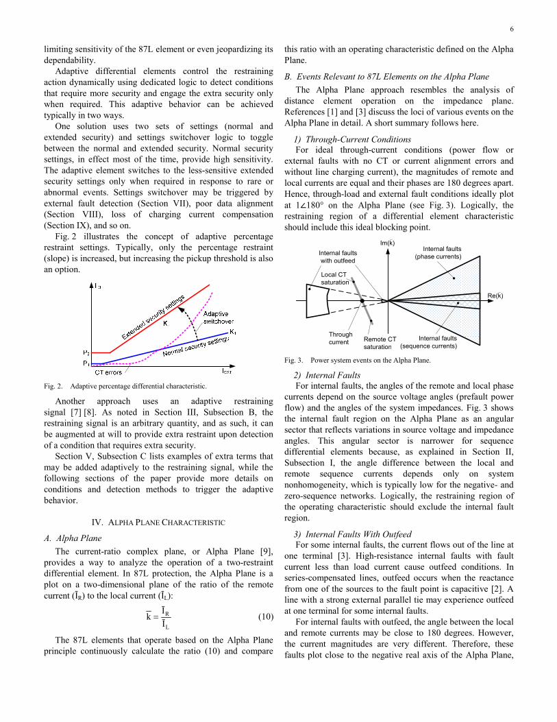
1) Through-Current Conditions For ideal through-current conditions (power flow or

external faults with no CT or current alignment errors and without line charging current), the magnitudes of remote and local currents are equal and their phases are 180 degrees apart. Hence, through-load and external fault conditions ideally plot at 1∠180° on the Alpha Plane (see Fig. 3). Logically, the restraining region of a differential element characteristic should include this ideal blocking point.

Re(k)

Internal faults(sequence currents)

Internal faults(phase currents)

Im(k)

Throughcurrent

Local CT saturation

Remote CT saturation

Internal faultswith outfeed

Fig. 3. Power system events on the Alpha Plane.

2) Internal Faults For internal faults, the angles of the remote and local phase

currents depend on the source voltage angles (prefault power flow) and the angles of the system impedances. Fig. 3 shows the internal fault region on the Alpha Plane as an angular sector that reflects variations in source voltage and impedance angles. This angular sector is narrower for sequence differential elements because, as explained in Section II, Subsection I, the angle difference between the local and remote sequence currents depends only on system nonhomogeneity, which is typically low for the negative- and zero-sequence networks. Logically, the restraining region of the operating characteristic should exclude the internal fault region.

3) Internal Faults With Outfeed For some internal faults, the current flows out of the line at

one terminal [3]. High-resistance internal faults with fault current less than load current cause outfeed conditions. In series-compensated lines, outfeed occurs when the reactance from one of the sources to the fault point is capacitive [2]. A line with a strong external parallel tie may experience outfeed at one terminal for some internal faults.

For internal faults with outfeed, the angle between the local and remote currents may be close to 180 degrees. However, the current magnitudes are very different. Therefore, these faults plot close to the negative real axis of the Alpha Plane,

7

but away from the 1∠180° point (Fig. 3). Logically, the restraining region of the operating characteristic should exclude the regions corresponding to internal faults with outfeed.

4) CT Saturation During External Faults When a CT saturates, the fundamental frequency

component of the secondary current decreases in magnitude and advances in angle.

We consider the phase differential elements first. When the local CT saturates and the CT at the remote end of the protected line does not saturate, the current-ratio magnitude of the phase currents increases and its phase angle decreases, moving the operating point upward and to the left from the 1∠180° point (Fig. 3). When the remote CT saturates and the local CT does not saturate, the current-ratio magnitude decreases and its phase angle increases, moving the operating point downward and to the right. Because of the effect of the current dc offset on CT saturation and the relay filtering transients, the current ratio actually describes a time-dependent irregular trajectory. Section VII provides more details and shows transient CT saturation trajectories. Logically, the restraining region of the operating characteristic should include the current ratios corresponding to external faults with CT saturation.

The impact of CT saturation on the sequence current ratio is far more complex than just a relatively well-defined shift from the 1∠180° point. The sequence current ratio is a function of six phasors for a two-restraint differential zone and depends on the fault type and amount of CT saturation in any of the up to six CTs that may carry fault current. Section VII further discusses this topic.

5) CT Saturation During Internal Faults Similar phenomena take place during internal faults. CT

saturation alters the phase current-ratio magnitude and angle, shifting the operating point from the expected internal fault position as defined by the source voltage angles and the system impedances. Logically, the restraining region of the operating characteristic should exclude the current ratios corresponding to internal faults with CT saturation.

6) Line Charging Current As explained in Section II, Subsection B, the differential

scheme measures the line charging current as a differential signal. Considering the charging current alone, the Alpha Plane element response to the charging current is very similar to that of internal faults. The current-ratio magnitude may vary considerably depending on the system impedances and reactive power sources in the vicinity of the line. This variation includes an ultimate case of an open breaker or a very weak system, leading to a current-ratio magnitude of zero or infinity. At the same time, the angles of the charging current contributions from both ends of the line are similar, placing the current ratio close to the positive real axis of the Alpha Plane.

When considering both the through current (load or external faults) and the charging current, the phase current ratio stays relatively close to the 1∠180° point, shifting more from this point when the charging current becomes a larger portion of the through current. The through current limits the impact of the charging current, providing the Alpha Plane elements with some security.

Sequence currents must be discussed separately, however. Under symmetrical conditions, there is no (or very small) standing sequence charging current. There is no (or very small) through sequence current either. Therefore, there is no stabilizing effect from the through current for the sequence current ratio, but that stabilizing effect is not required anyway.

However, sequence charging currents may appear under unbalanced conditions. Line energization (a single-end feed) creates challenges for any differential element. On the Alpha Plane, the single-end feed causes the current ratio to be zero or infinity, depending on if the local or remote terminal picks up the line.

Section IX discusses solutions to the line charging current challenges.

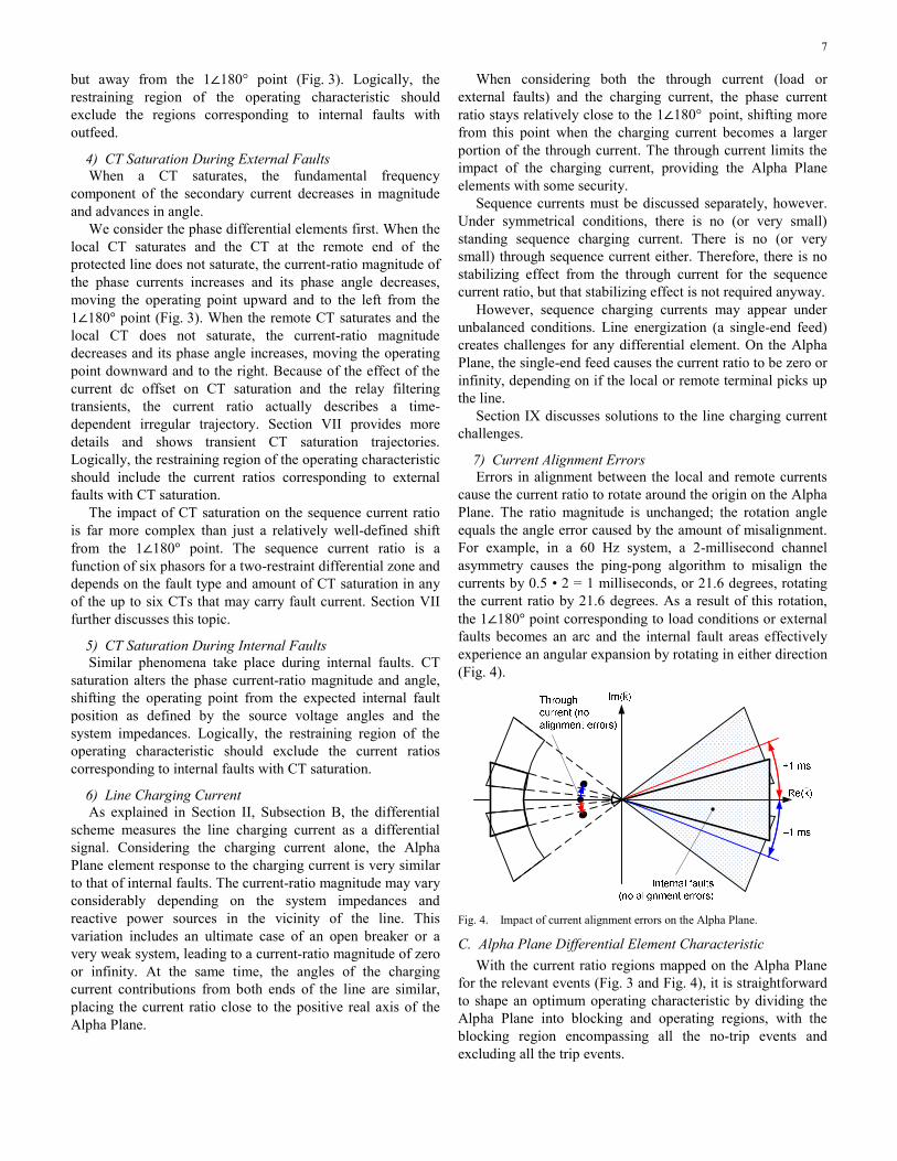
7) Current Alignment Errors Errors in alignment between the local and remote currents

cause the current ratio to rotate around the origin on the Alpha Plane. The ratio magnitude is unchanged; the rotation angle equals the angle error caused by the amount of misalignment. For example, in a 60 Hz system, a 2-millisecond channel asymmetry causes the ping-pong algorithm to misalign the currents by 0.5 • 2 = 1 milliseconds, or 21.6 degrees, rotating the current ratio by 21.6 degrees. As a result of this rotation, the 1∠180° point corresponding to load conditions or external faults becomes an arc and the internal fault areas effectively experience an angular expansion by rotating in either direction (Fig. 4).

Fig. 4. Impact of current alignment errors on the Alpha Plane.

C. Alpha Plane Differential Element Characteristic With the current ratio regions mapped on the Alpha Plane

for the relevant events (Fig. 3 and Fig. 4), it is straightforward to shape an optimum operating characteristic by dividing the Alpha Plane into blocking and operating regions, with the blocking region encompassing all the no-trip events and excluding all the trip events.

8

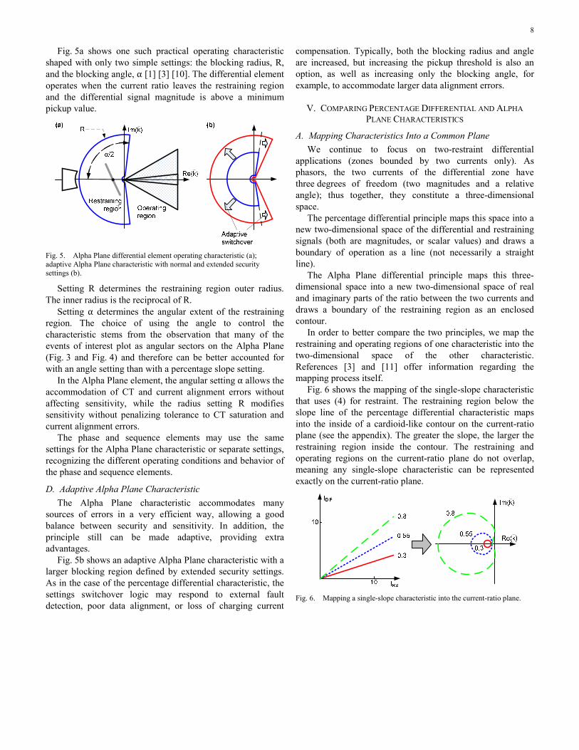
Fig. 5a shows one such practical operating characteristic shaped with only two simple settings: the blocking radius, R, and the blocking angle, α [1] [3] [10]. The differential element operates when the current ratio leaves the restraining region and the differential signal magnitude is above a minimum pickup value.

Fig. 5. Alpha Plane differential element operating characteristic (a); adaptive Alpha Plane characteristic with normal and extended security settings (b).

Setting R determines the restraining region outer radius. The inner radius is the reciprocal of R.

Setting α determines the angular extent of the restraining region. The choice of using the angle to control the characteristic stems from the observation that many of the events of interest plot as angular sectors on the Alpha Plane (Fig. 3 and Fig. 4) and therefore can be better accounted for with an angle setting than with a percentage slope setting.

In the Alpha Plane element, the angular setting α allows the accommodation of CT and current alignment errors without affecting sensitivity, while the radius setting R modifies sensitivity without penalizing tolerance to CT saturation and current alignment errors.

The phase and sequence elements may use the same settings for the Alpha Plane characteristic or separate settings, recognizing the different operating conditions and behavior of the phase and sequence elements.

D. Adaptive Alpha Plane Characteristic The Alpha Plane characteristic accommodates many

sources of errors in a very efficient way, allowing a good balance between security and sensitivity. In addition, the principle still can be made adaptive, providing extra advantages.

Fig. 5b shows an adaptive Alpha Plane characteristic with a larger blocking region defined by extended security settings. As in the case of the percentage differential characteristic, the settings switchover logic may respond to external fault detection, poor data alignment, or loss of charging current

compensation. Typically, both the blocking radius and angle are increased, but increasing the pickup threshold is also an option, as well as increasing only the blocking angle, for example, to accommodate larger data alignment errors.

V. COMPARING PERCENTAGE DIFFERENTIAL AND ALPHA PLANE CHARACTERISTICS

A. Mapping Characteristics Into a Common Plane We continue to focus on two-restraint differential

applications (zones bounded by two currents only). As phasors, the two currents of the differential zone have three degrees of freedom (two magnitudes and a relative angle); thus together, they constitute a three-dimensional space.

The percentage differential principle maps this space into a new two-dimensional space of the differential and restraining signals (both are magnitudes, or scalar values) and draws a boundary of operation as a line (not necessarily a straight line).

The Alpha Plane differential principle maps this three-dimensional space into a new two-dimensional space of real and imaginary parts of the ratio between the two currents and draws a boundary of the restraining region as an enclosed contour.

In order to better compare the two principles, we map the restraining and operating regions of one characteristic into the two-dimensional space of the other characteristic. References [3] and [11] offer information regarding the mapping process itself.

Fig. 6 shows the mapping of the single-slope characteristic that uses (4) for restraint. The restraining region below the slope line of the percentage differential characteristic maps into the inside of a cardioid-like contour on the current-ratio plane (see the appendix). The greater the slope, the larger the restraining region inside the contour. The restraining and operating regions on the current-ratio plane do not overlap, meaning any single-slope characteristic can be represented exactly on the current-ratio plane.

Fig. 6. Mapping a single-slope characteristic into the current-ratio plane.

9

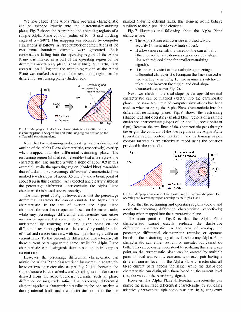
We now check if the Alpha Plane operating characteristic can be mapped exactly into the differential-restraining plane. Fig. 7 shows the restraining and operating regions of a sample Alpha Plane contour (radius of R = 3 and blocking angle of α = 240°). This mapping was obtained by computer simulations as follows. A large number of combinations of the two zone boundary currents were generated. Each combination falling into the operating region of the Alpha Plane was marked as a part of the operating region on the differential-restraining plane (shaded blue). Similarly, each combination falling into the restraining region of the Alpha Plane was marked as a part of the restraining region on the differential-restraining plane (shaded red).

IRST

IDIF

10

10

Re(k)

Im(k)

Restraining and operating regions overlap

–1

RestrainOperate

ab

Fig. 7. Mapping an Alpha Plane characteristic into the differential-restraining plane. The operating and restraining regions overlap on the differential-restraining plane.

Note that the restraining and operating regions (inside and outside of the Alpha Plane characteristic, respectively) overlap when mapped into the differential-restraining plane. The restraining region (shaded red) resembles that of a single-slope characteristic (line marked a with a slope of about 0.9 in this example), while the operating region (shaded blue) resembles that of a dual-slope percentage differential characteristic (line marked b with slopes of about 0.5 and 0.9 and a break point of about 8 pu in this example). As expected and clearly visible in the percentage differential characteristic, the Alpha Plane characteristic is biased toward security.

The main point of Fig. 7, however, is that the percentage differential characteristic cannot emulate the Alpha Plane characteristic. In the area of overlap, the Alpha Plane characteristic restrains or operates based on the current ratio, while any percentage differential characteristic can either restrain or operate, but cannot do both. This can be easily understood by realizing that any given point on the differential-restraining plane can be created by multiple pairs of local and remote currents, with each pair having a different current ratio. To the percentage differential characteristic, all these current pairs appear the same, while the Alpha Plane characteristic can distinguish them based on their complex current ratio.

However, the percentage differential characteristic can mimic the Alpha Plane characteristic by switching adaptively between two characteristics as per Fig. 7 (i.e., between the slope characteristics marked a and b), using extra information derived from the zone boundary currents, such as phase difference or magnitude ratio. If a percentage differential element applied a characteristic similar to the one marked a during internal faults and a characteristic similar to the one

marked b during external faults, this element would behave similarly to the Alpha Plane element.

Fig. 7 illustrates the following about the Alpha Plane characteristic:

• The Alpha Plane characteristic is biased toward security (it maps into very high slopes).

• It allows more sensitivity based on the current ratio (the unconditional restraining region is a dual-slope line with reduced slope for smaller restraining signals).

• It is inherently similar to an adaptive percentage differential characteristic (compare the lines marked a and b in Fig. 7 with Fig. 1b, and assume a switchover takes place between the single- and dual-slope characteristics as per Fig. 2).

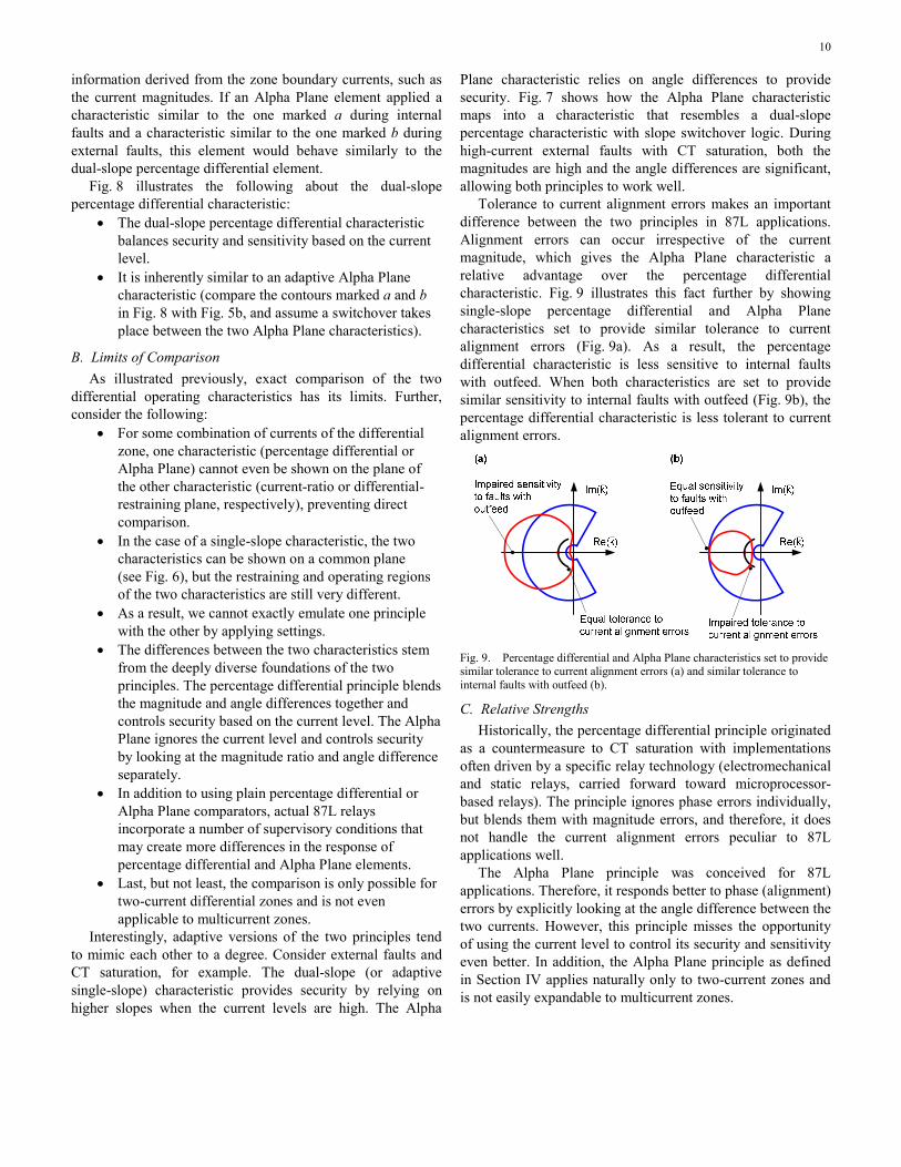
Next, we check if the dual-slope percentage differential characteristic can be mapped exactly into the current-ratio plane. The same technique of computer simulations has been used as when mapping the Alpha Plane characteristic into the differential-restraining plane. Fig. 8 shows the restraining (shaded red) and operating (shaded blue) regions of a sample dual-slope characteristic (slopes of 0.5 and 0.7, break point of 6 pu). Because the two lines of the characteristic pass through the origin, the contours of the two regions in the Alpha Plane (operating region contour marked a and restraining region contour marked b) are effectively traced using the equation provided in the appendix.

Fig. 8. Mapping a dual-slope characteristic into the current-ratio plane. The operating and restraining regions overlap on the Alpha Plane.

Note that the restraining and operating regions (below and above the percentage differential characteristic, respectively) overlap when mapped into the current-ratio plane.

The main point of Fig. 8 is that the Alpha Plane characteristic cannot exactly replicate the dual-slope differential characteristic. In the area of overlap, the percentage differential characteristic restrains or operates based on the restraining signal level, while any Alpha Plane characteristic can either restrain or operate, but cannot do both. This can be easily understood by realizing that any given point on the current-ratio plane can be created by multiple pairs of local and remote currents, with each pair having a different current level. To the Alpha Plane characteristic, all these current pairs appear the same, while the dual-slope characteristic can distinguish them based on the current level (i.e., the value of the restraining signal).

However, the Alpha Plane differential characteristic can mimic the percentage differential characteristic by switching adaptively between multiple contours as per Fig. 8, using extra

10

information derived from the zone boundary currents, such as the current magnitudes. If an Alpha Plane element applied a characteristic similar to the one marked a during internal faults and a characteristic similar to the one marked b during external faults, this element would behave similarly to the dual-slope percentage differential element.

Fig. 8 illustrates the following about the dual-slope percentage differential characteristic:

• The dual-slope percentage differential characteristic balances security and sensitivity based on the current level.

• It is inherently similar to an adaptive Alpha Plane characteristic (compare the contours marked a and b in Fig. 8 with Fig. 5b, and assume a switchover takes place between the two Alpha Plane characteristics).

B. Limits of Comparison As illustrated previously, exact comparison of the two

differential operating characteristics has its limits. Further, consider the following:

• For some combination of currents of the differential zone, one characteristic (percentage differential or Alpha Plane) cannot even be shown on the plane of the other characteristic (current-ratio or differential-restraining plane, respectively), preventing direct comparison.

• In the case of a single-slope characteristic, the two characteristics can be shown on a common plane (see Fig. 6), but the restraining and operating regions of the two characteristics are still very different.

• As a result, we cannot exactly emulate one principle with the other by applying settings.

• The differences between the two characteristics stem from the deeply diverse foundations of the two principles. The percentage differential principle blends the magnitude and angle differences together and controls security based on the current level. The Alpha Plane ignores the current level and controls security by looking at the magnitude ratio and angle difference separately.

• In addition to using plain percentage differential or Alpha Plane comparators, actual 87L relays incorporate a number of supervisory conditions that may create more differences in the response of percentage differential and Alpha Plane elements.

• Last, but not least, the comparison is only possible for two-current differential zones and is not even applicable to multicurrent zones.

Interestingly, adaptive versions of the two principles tend to mimic each other to a degree. Consider external faults and CT saturation, for example. The dual-slope (or adaptive single-slope) characteristic provides security by relying on higher slopes when the current levels are high. The Alpha

Plane characteristic relies on angle differences to provide security. Fig. 7 shows how the Alpha Plane characteristic maps into a characteristic that resembles a dual-slope percentage characteristic with slope switchover logic. During high-current external faults with CT saturation, both the magnitudes are high and the angle differences are significant, allowing both principles to work well.

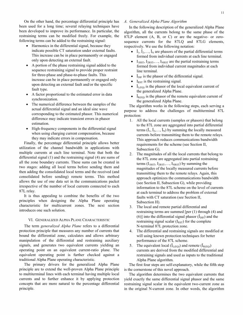
Tolerance to current alignment errors makes an important difference between the two principles in 87L applications. Alignment errors can occur irrespective of the current magnitude, which gives the Alpha Plane characteristic a relative advantage over the percentage differential characteristic. Fig. 9 illustrates this fact further by showing single-slope percentage differential and Alpha Plane characteristics set to provide similar tolerance to current alignment errors (Fig. 9a). As a result, the percentage differential characteristic is less sensitive to internal faults with outfeed. When both characteristics are set to provide similar sensitivity to internal faults with outfeed (Fig. 9b), the percentage differential characteristic is less tolerant to current alignment errors.

Fig. 9. Percentage differential and Alpha Plane characteristics set to provide similar tolerance to current alignment errors (a) and similar tolerance to internal faults with outfeed (b).

C. Relative Strengths Historically, the percentage differential principle originated

as a countermeasure to CT saturation with implementations often driven by a specific relay technology (electromechanical and static relays, carried forward toward microprocessor-based relays). The principle ignores phase errors individually, but blends them with magnitude errors, and therefore, it does not handle the current alignment errors peculiar to 87L applications well.

The Alpha Plane principle was conceived for 87L applications. Therefore, it responds better to phase (alignment) errors by explicitly looking at the angle difference between the two currents. However, this principle misses the opportunity of using the current level to control its security and sensitivity even better. In addition, the Alpha Plane principle as defined in Section IV applies naturally only to two-current zones and is not easily expandable to multicurrent zones.

11

On the other hand, the percentage differential principle has been used for a long time; several relaying techniques have been developed to improve its performance. In particular, the restraining terms can be modified freely. For example, the following terms can be added to the restraining signal:

• Harmonics in the differential signal, because they indicate possible CT saturation under external faults. This increase can be in place permanently or engaged only upon detecting an external fault.

• A portion of the phase restraining signal added to the sequence restraining signal to provide proper restraint for three-phase and phase-to-phase faults. This increase can be in place permanently or engaged only upon detecting an external fault and/or the specific fault type.

• A factor proportional to the estimated error in data synchronization.

• The numerical difference between the samples of the actual differential signal and an ideal sine wave corresponding to the estimated phasor. This numerical difference may indicate transient errors in phasor estimation.

• High-frequency components in the differential signal when using charging current compensation, because they may indicate errors in compensation.

Finally, the percentage differential principle allows better utilization of the channel bandwidth in applications with multiple currents at each line terminal. Note that both the differential signal (1) and the restraining signal (4) are sums of all the zone boundary currents. These sums can be created in two stages: adding all local terms before sending them and then adding the consolidated local terms and the received (and consolidated before sending) remote terms. This method allows the use of one data set in the communications packet irrespective of the number of local currents connected to each 87L relay.

It is thus appealing to combine the benefits of the two principles when designing the Alpha Plane operating characteristic for multicurrent zones. The next section introduces one such solution.

VI. GENERALIZED ALPHA PLANE CHARACTERISTIC The term generalized Alpha Plane refers to a differential

protection principle that measures any number of currents that bound the differential zone, calculates and allows arbitrary manipulation of the differential and restraining auxiliary signals, and generates two equivalent currents yielding an operating point on an equivalent current-ratio plane. The equivalent operating point is further checked against a traditional Alpha Plane operating characteristic.

The primary drivers for the generalized Alpha Plane principle are to extend the well-proven Alpha Plane principle to multiterminal lines with each terminal having multiple local currents and to further enhance it by applying protection concepts that are more natural to the percentage differential principle.

A. Generalized Alpha Plane Algorithm In the following description of the generalized Alpha Plane

algorithm, all the currents belong to the same phase of the 87LP element (A, B, or C) or are the negative- or zero-sequence currents for the 87LQ and 87LG elements, respectively. We use the following notation:

• Ī1, Ī2,…, ĪN are phasors of the partial differential terms formed from individual currents at each line terminal.

• I1RST, I2RST,…, INRST are the partial restraining terms formed from individual current magnitudes at each line terminal.

• ĪDIF is the phasor of the differential signal. • IRST is the restraining signal. • ĪL(EQ) is the phasor of the local equivalent current of

the generalized Alpha Plane. • ĪR(EQ) is the phasor of the remote equivalent current of

the generalized Alpha Plane. The algorithm works in the following steps, each serving a

purpose to address the challenges of multiterminal 87L protection:

1. All the local currents (samples or phasors) that belong to the 87L zone are aggregated into partial differential terms (Ī1, Ī2,…, ĪN) by summing the locally measured currents before transmitting them to the remote relays. This approach reduces communications bandwidth requirements for the scheme (see Section II, Subsection G).

2. The magnitudes of all the local currents that belong to the 87L zone are aggregated into partial restraining terms (I1RST, I2RST,…, INRST) by summing the magnitudes of the locally measured currents before transmitting them to the remote relays. Again, this approach optimizes the communications bandwidth (see Section II, Subsection G), while providing information to the 87L scheme on the level of currents at each terminal to address the problem of external faults with CT saturation (see Section II, Subsection H).

3. The local and remote partial differential and restraining terms are summed [per (1) through (4) and (6)] into the differential signal phasor (ĪDIF) and the restraining signal scalar (IRST) for the complete N-terminal 87L protection zone.

4. The differential and restraining signals are modified at will using known protection techniques for better performance of the 87L scheme.

5. The equivalent local (ĪL(EQ)) and remote (ĪR(EQ)) currents are derived from the modified differential and restraining signals and used as inputs to the traditional Alpha Plane algorithm.

The first four steps are self-explanatory, while the fifth step is the cornerstone of this novel approach.

The algorithm determines the two equivalent currents that yield exactly the same differential signal phasor and the same restraining signal scalar in the equivalent two-current zone as in the original N-current zone. In other words, the algorithm

12

design starts with the following question: Which are the two equivalent currents that yield exactly the same differential and restraining signals as the actual N-current zone? The problem is solved analytically during the algorithm design phase (as shown in the next paragraphs), and the resulting solution is programmed in a microprocessor-based relay and executed in real time during relay operation.

The algorithm design is constrained with three equations; the real and imaginary parts of the differential signal and the magnitude of the restraining signal from the two equivalent currents must match the actual values of the 87L zone. At the same time, the algorithm seeks to obtain four unknowns: the real and imaginary parts of the two equivalent currents. As a result, the problem has more variables than equations.

One specific approach avoids using a fourth equation by selecting the angular position of one of the equivalent currents to align the equivalent current with a specific actual zone boundary current [8]. That specific zone boundary current is the one that has the largest projection on the differential signal phasor.

The rationale supporting this solution is as follows. During external faults, it is preferable to select the current flowing out of the 87L zone as one of the equivalent currents. Because of CT saturation, the highest current is not necessarily the current flowing out of the protection zone toward the external fault. However, CT saturation would yield an error signal in this current that is relatively in phase with the external fault current (angle difference up to 90 degrees in an ultimate case of extreme saturation). This error signal would demonstrate itself as a fictitious differential signal, assuming all other CTs work without saturation (the worst-case scenario). As a result, the secondary external fault current (including the effect of CT saturation) is relatively in phase with the differential signal in addition to being significant (unless extreme CT saturation brings the magnitude of the secondary current down). Therefore, looking at the angles between each of the zone boundary currents and the differential signal helps in identifying the external fault current.

To this end, the following auxiliary signals are calculated:

( )k k DIFR Re Ī • Ī∗= (11)

where: * stands for a complex conjugate operation. k is 1..N.

The zone boundary current Īk that yields the highest Rk value is selected as an angular reference for one of the two equivalent Alpha Plane currents:

( )kArg Īβ = (12)

Next, an auxiliary phasor ĪX is calculated by shifting the differential signal by the angle β:

( )X DIFĪ Ī •1= ∠ −β (13)

Now, the following two equivalent currents can be calculated [8]:

( )

( ) ( )( )( )( ) ( )

L EQ

22X RST X

XRST X

Ī

Im Ī I Re Īj • Im Ī •1

2 • I Re Ī

=

⎛ ⎞− −⎜ ⎟+ ∠β⎜ ⎟−⎝ ⎠

(14)

( ) ( )( )RSTR EQ L EQĪ I Ī •1= − ∠β (15)

The generalized Alpha Plane algorithm derives the complex ratio of the two equivalent currents calculated per (14) and (15) and applies it to the operating characteristic. These internal calculations are performed independently for the A-phase, B-phase, C-phase, negative-sequence, and zero-sequence currents.

The following two examples illustrate the generalized Alpha Plane calculations using (11) through (15).

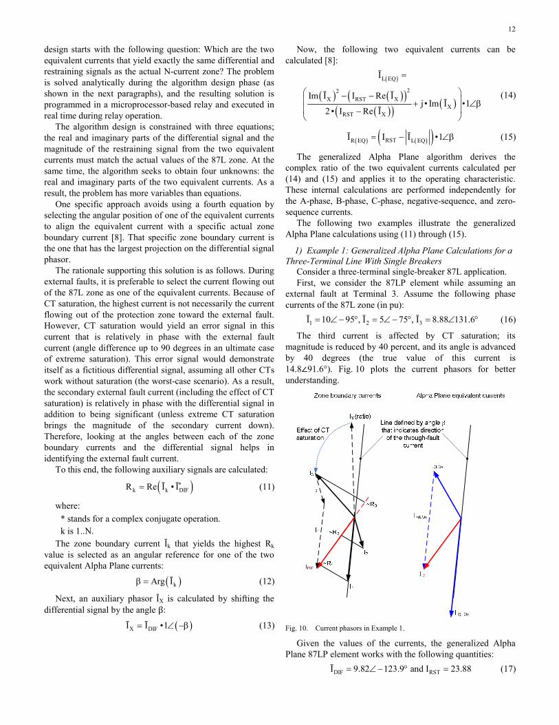
1) Example 1: Generalized Alpha Plane Calculations for a Three-Terminal Line With Single Breakers

Consider a three-terminal single-breaker 87L application. First, we consider the 87LP element while assuming an

external fault at Terminal 3. Assume the following phase currents of the 87L zone (in pu): 1 2 3Ī 10 95 , Ī 5 75 , Ī 8.88 131.6= ∠− ° = ∠− ° = ∠ ° (16)

The third current is affected by CT saturation; its magnitude is reduced by 40 percent, and its angle is advanced by 40 degrees (the true value of this current is 14.8∠91.6°). Fig. 10 plots the current phasors for better understanding.

Fig. 10. Current phasors in Example 1.

Given the values of the currents, the generalized Alpha Plane 87LP element works with the following quantities: DIF RSTĪ 9.82 123.9 and I 23.88= ∠− ° = (17)

13

The Rk values for the three currents as per (11) are 86.0, 32.3, and 21.8, respectively. The algorithm selects the Terminal 1 current Ī1 as the reference (the highest Rk). Therefore, β = –95° per (12). This selection is rational because, in this case, the bulk of the fault current flows between Terminals 1 and 3 (i.e., along the line of about ±90 degrees).

Using (14) and (15), the algorithm calculates: ( ) ( )L EQ R EQĪ 8.38 119.5 and Ī 15.50 95= ∠ ° = ∠− ° (18)

The complex ratio between the two equivalent currents is:

k 1.85 145= ∠ ° (19) An Alpha Plane characteristic with a blocking angle of at

least 70 degrees (the typical setting is around 180 degrees) would qualify this condition as an external fault.

By comparison, the percentage differential characteristic would need a slope of at least 9.82/23.88, or 41.1 percent in order to remain secure for this external fault.

We now apply a traditional two-current Alpha Plane concept to this three-terminal line. In one approach [3], all possible fault locations are considered and a separate current ratio is derived for each of the combinations. In this example, the following ratios are checked:

• Ī1 versus Ī2 + Ī3, yielding the ratio of 2.02∠106.4° (assumes an external fault at Terminal 1).

• Ī2 versus Ī1 + Ī3, yielding the ratio of 1.51∠–78.8° (assumes an external fault at Terminal 2).

• Ī3 versus Ī1 + Ī2, yielding the ratio of 1.66∠140° (assumes an external fault at Terminal 3).

Note that the blocking angle has the largest impact on security, and therefore, the third combination with the ratio of 1.66∠140° is the most appropriate. This result is expected because the external fault is truly at Terminal 3. The generalized Alpha Plane algorithm returned the ratio of 1.85∠145°. This value is a similar but slightly better value (considering protection security) and was obtained without exercising all possible fault locations.

Next, we consider the 87LQ element while assuming an internal fault. Assume the following negative-sequence currents (in pu): 1Q 2Q 3QĪ 2 87 , Ī 3 85 , Ī 1 82= ∠− ° = ∠− ° = ∠− ° (20)

The currents have similar phase angles, which reflects the homogeneity of the negative-sequence network.

The generalized Alpha Plane 87LQ element works with the following quantities: DIF RSTĪ 6 85.2 and I 6= ∠− ° = (21)

The Rk values are 12.0, 18.0, and 6.0, respectively. The algorithm selects the Terminal 2 current Ī2Q as the reference (the highest Rk). Therefore, β = –85°. This selection is of secondary importance as all the fault currents flow along the same line of about –85 degrees.

Using (14) and (15), the algorithm calculates: ( ) ( )L EQ R EQĪ 0.06 101.9 and Ī 5.94 85= ∠− ° = ∠− ° (22)

The complex ratio between the two equivalent currents is:

k 98.7 16.9= ∠ ° (23) Any Alpha Plane characteristic set rationally would qualify

this condition as an internal fault. When a given line terminal is a dual-breaker connection,

the remote relays working with the partial differential and partial restraining terms do not have access to the individual phasors of the two currents, but only to their sums (partial terms). This is only a minor limitation to the effectiveness of the generalized Alpha Plane algorithm because its strength results from reflecting the differential and through currents of the zone and these two signals are always represented correctly. The following example illustrates this point better.

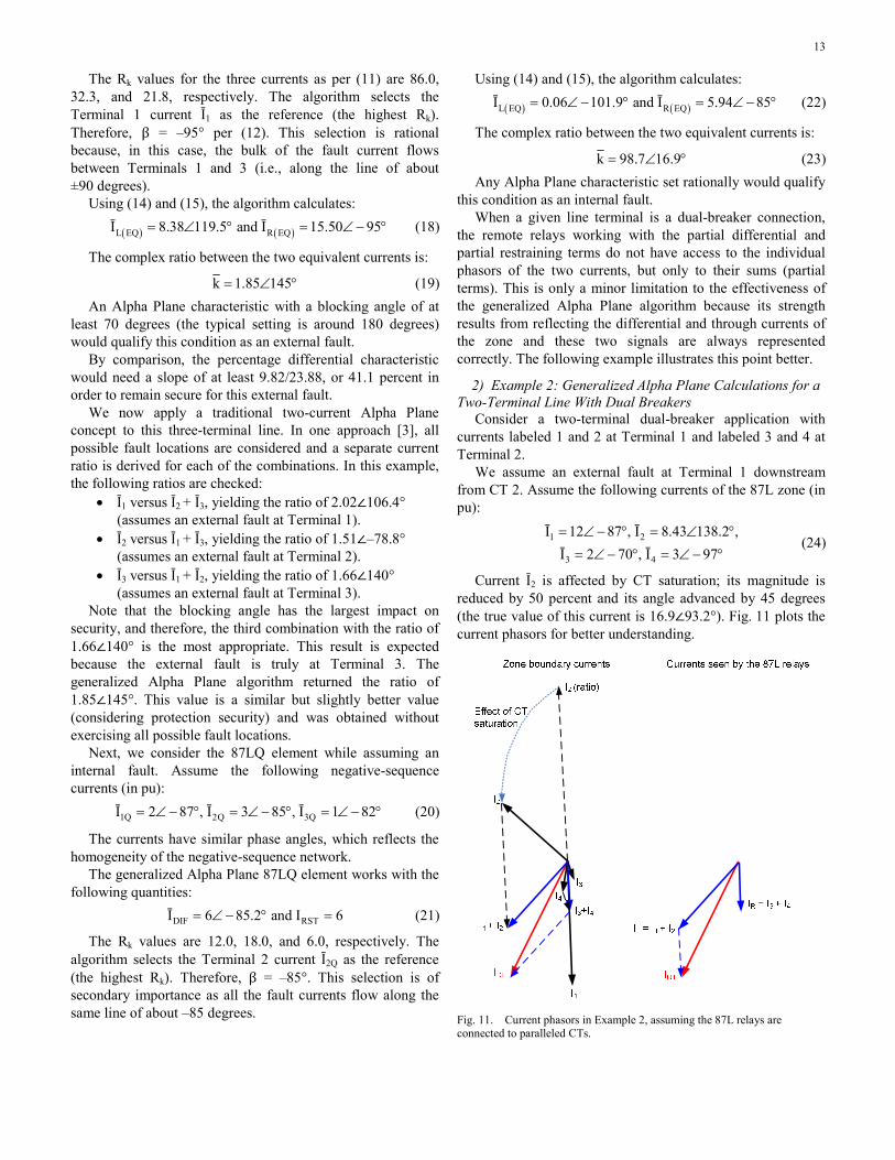
2) Example 2: Generalized Alpha Plane Calculations for a Two-Terminal Line With Dual Breakers

Consider a two-terminal dual-breaker application with currents labeled 1 and 2 at Terminal 1 and labeled 3 and 4 at Terminal 2.

We assume an external fault at Terminal 1 downstream from CT 2. Assume the following currents of the 87L zone (in pu):

1 2

3 4

Ī 12 87 , Ī 8.43 138.2 ,Ī 2 70 , Ī 3 97= ∠− ° = ∠ °

= ∠− ° = ∠− ° (24)

Current Ī2 is affected by CT saturation; its magnitude is reduced by 50 percent and its angle advanced by 45 degrees (the true value of this current is 16.9∠93.2°). Fig. 11 plots the current phasors for better understanding.

Fig. 11. Current phasors in Example 2, assuming the 87L relays are connected to paralleled CTs.

14

First, we consider 87L relays having single CT inputs and therefore wired to the two CTs at each terminal connected in parallel. These relays measure the following currents:

L 1 2

R 3 4

I Ī Ī 8.52 131.7 at Terminal 1;I Ī Ī 4.87 86.2 at Terminal 2

= + = ∠− °

= + = ∠− ° (25)

The differential signal is: DIFĪ 12.4 115.5= ∠− ° (26)

The percentage differential element works with a restraining signal of IRST = 8.52 + 4.87 = 13.4 and therefore requires a slope of at least 12.4/13.4, or 92.5 percent, for security.

The Alpha Plane element works with the complex current ratio of:

( )( )8.52 131.7

k 1.75 45.44.87 86.2

∠− °= = ∠− °

∠− ° (27)

and requires a blocking angle of at least 272 degrees for security.

Both the percentage differential and the Alpha Plane elements would have difficulties providing security in this case. The reason is that these elements are connected to the paralleled CTs and are not aware of the large through-fault current that flows in and out of the line protection zone at Terminal 1.

We now consider the generalized Alpha Plane elements in 87L relays with dual CT inputs that measure both currents at each line terminal. The partial terms are:

1 2

1 2

1 2

1 2

Terminal 1, differential: Ī Ī 12 87 8.43 138.2 8.52 131.7 ,

Terminal 1, restraining: I I 12 8.43 20.43,Terminal 2, differential:

Ī Ī 2 70 3 97 4.87 86.2 ,Terminal 2, restraining:

I I 2

+ = ∠− °+ ∠ ° = ∠− °

+ = + =

+ = ∠− ° + ∠− ° = ∠− °

+ = 3 5+ =

(28)

The generalized Alpha Plane element works with the following quantities: DIF RSTĪ 12.4 115.5 and I 25.43= ∠− ° = (29)

The Rk values are 101.6 and 52.8, respectively. The algorithm selects the Terminal 1 current Ī1 as the reference (the highest Rk). Therefore, β = –131.7°.

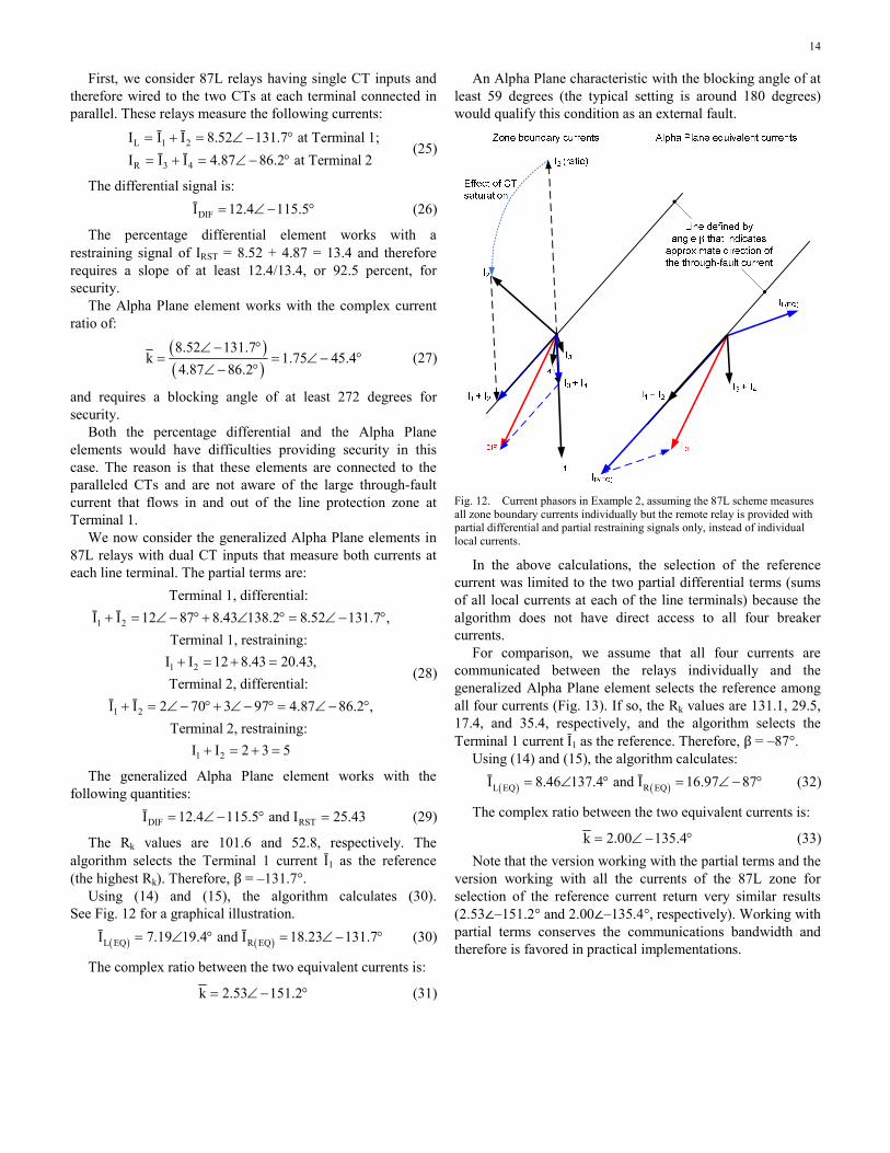
Using (14) and (15), the algorithm calculates (30). See Fig. 12 for a graphical illustration. ( ) ( )L EQ R EQĪ 7.19 19.4 and Ī 18.23 131.7= ∠ ° = ∠− ° (30)

The complex ratio between the two equivalent currents is:

k 2.53 151.2= ∠− ° (31)

An Alpha Plane characteristic with the blocking angle of at least 59 degrees (the typical setting is around 180 degrees) would qualify this condition as an external fault.

Fig. 12. Current phasors in Example 2, assuming the 87L scheme measures all zone boundary currents individually but the remote relay is provided with partial differential and partial restraining signals only, instead of individual local currents.

In the above calculations, the selection of the reference current was limited to the two partial differential terms (sums of all local currents at each of the line terminals) because the algorithm does not have direct access to all four breaker currents.

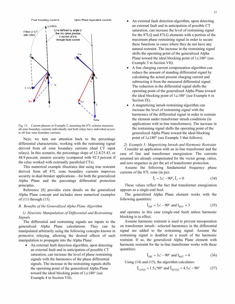
For comparison, we assume that all four currents are communicated between the relays individually and the generalized Alpha Plane element selects the reference among all four currents (Fig. 13). If so, the Rk values are 131.1, 29.5, 17.4, and 35.4, respectively, and the algorithm selects the Terminal 1 current Ī1 as the reference. Therefore, β = –87°.

Using (14) and (15), the algorithm calculates: ( ) ( )L EQ R EQĪ 8.46 137.4 and Ī 16.97 87= ∠ ° = ∠− ° (32)

The complex ratio between the two equivalent currents is:

k 2.00 135.4= ∠− ° (33) Note that the version working with the partial terms and the

version working with all the currents of the 87L zone for selection of the reference current return very similar results (2.53∠–151.2° and 2.00∠–135.4°, respectively). Working with partial terms conserves the communications bandwidth and therefore is favored in practical implementations.

15

Fig. 13. Current phasors in Example 2, assuming the 87L scheme measures all zone boundary currents individually and both relays have individual access to all four zone boundary currents.

Next, we turn our attention back to the percentage differential characteristic, working with the restraining signal derived from all zone boundary currents (dual CT input relays). In this scenario, the percentage slope of 12.4/25.43, or 48.9 percent, ensures security (compared with 92.5 percent if the relay worked with externally paralleled CTs).

This numerical example illustrates that using true restraint derived from all 87L zone boundary currents improves security in dual-breaker applications—for both the generalized Alpha Plane and the percentage differential protection principles.

Reference [8] provides extra details on the generalized Alpha Plane concept and includes more numerical examples of (11) through (15).

B. Benefits of the Generalized Alpha Plane Algorithm

1) Heuristic Manipulation of Differential and Restraining Signals

The differential and restraining signals are inputs to the generalized Alpha Plane calculations. They can be manipulated arbitrarily using the following concepts known in protective relaying, allowing the desired effects of such manipulation to propagate into the Alpha Plane:

• An external fault detection algorithm, upon detecting an external fault and in anticipation of possible CT saturation, can increase the level of phase restraining signals with the harmonics of the phase differential signals. The increase in the restraining signals shifts the operating point of the generalized Alpha Plane toward the ideal blocking point of 1∠180° (see Example 4 in Section VII).

• An external fault detection algorithm, upon detecting an external fault and in anticipation of possible CT saturation, can increase the level of restraining signal for the 87LQ and 87LG elements with a portion of the maximum phase restraining signal in order to secure these functions in cases where they do not have any natural restraint. The increase in the restraining signal shifts the operating point of the generalized Alpha Plane toward the ideal blocking point of 1∠180° (see Example 5 in Section VII).

• A line charging current compensation algorithm can reduce the amount of standing differential signal by calculating the actual present charging current and subtracting it from the measured differential signal. The reduction in the differential signal shifts the operating point of the generalized Alpha Plane toward the ideal blocking point of 1∠180° (see Example 6 in Section IX).

• A magnetizing inrush restraining algorithm can increase the level of restraining signal with the harmonics of the differential signal in order to restrain the element under transformer inrush conditions (in applications with in-line transformers). The increase in the restraining signal shifts the operating point of the generalized Alpha Plane toward the ideal blocking point of 1∠180° (see Example 3 that follows).

2) Example 3: Magnetizing Inrush and Harmonic Restraint Consider an application with an in-line transformer and the

case of line and transformer energization. The currents assumed are already compensated for the vector group, ratios, and zero sequence as per the art of transformer protection.

Assume the following fundamental frequency phase currents of the 87L zone (in pu): 1 2Ī 3 90 , Ī 0= ∠− ° = (34)

These values reflect the fact that transformer energization appears as a single-end feed.

The generalized Alpha Plane element works with the following quantities: DIF RSTĪ 3 90 and I 3= ∠− ° = (35)

and operates in this case (single-end feed) unless harmonic blocking is in effect.

Assume harmonic restraint is used to prevent misoperation on transformer inrush—selected harmonics in the differential signal are added to the restraining signal. Assume the restraining signal is doubled as a result of the harmonic restraint. If so, the generalized Alpha Plane element with harmonic restraint for the in-line transformer works with these quantities: DIF RSTĪ 3 90 and I 6= ∠− ° = (36)

Using (14) and (15), the algorithm calculates: ( ) ( )L EQ R EQĪ 1.5 90 and Ī 4.5 90= ∠ ° = ∠− ° (37)

16

As a result of augmenting the restraining signal, both equivalent currents are not zero (unlike the actual currents), allowing the element to restrain. The complex ratio between the two equivalent currents is:

k 3 180= ∠ ° (38) This operating point is safely within the blocking region of

a typical Alpha Plane characteristic, allowing the element to restrain properly.

In summary, having an intermediate layer of differential and restraining signals before transitioning into the Alpha Plane calculations allows the application of tried-and-true protection concepts and maximizes the advantages of both the traditional percentage differential and Alpha Plane principles.

VII. ENHANCING DIFFERENTIAL ELEMENT SECURITY FOR CT SATURATION

Previous sections of this paper pointed out that CT saturation causes a fictitious differential signal and suggested methods for enhancing 87L element security. In this section, we further analyze this problem, describe various solutions in more detail, and illustrate the discussion with numerical examples, including transient simulation studies.

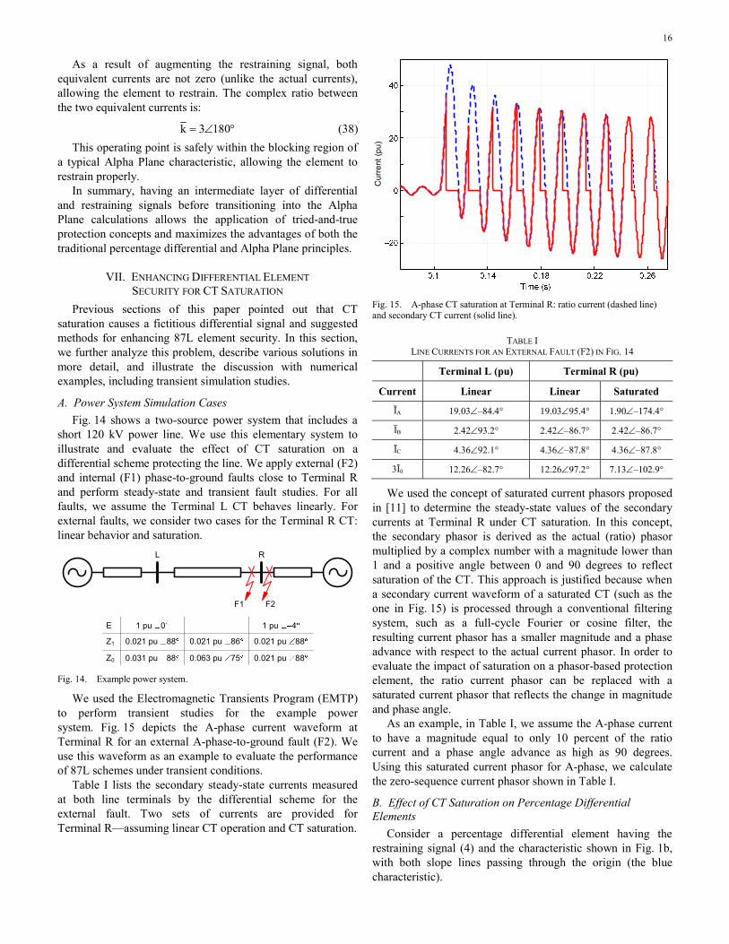
A. Power System Simulation Cases Fig. 14 shows a two-source power system that includes a

short 120 kV power line. We use this elementary system to illustrate and evaluate the effect of CT saturation on a differential scheme protecting the line. We apply external (F2) and internal (F1) phase-to-ground faults close to Terminal R and perform steady-state and transient fault studies. For all faults, we assume the Terminal L CT behaves linearly. For external faults, we consider two cases for the Terminal R CT: linear behavior and saturation.

L R

F1 F2

Z1

Z0

0.021 pu 88

0.021 pu 88

0.021 pu 86

0.063 pu 75

E 1 pu 4

0.021 pu 88

0.031 pu 88

1 pu 0

Fig. 14. Example power system.

We used the Electromagnetic Transients Program (EMTP) to perform transient studies for the example power system. Fig. 15 depicts the A-phase current waveform at Terminal R for an external A-phase-to-ground fault (F2). We use this waveform as an example to evaluate the performance of 87L schemes under transient conditions.

Table I lists the secondary steady-state currents measured at both line terminals by the differential scheme for the external fault. Two sets of currents are provided for Terminal R—assuming linear CT operation and CT saturation.

Cur

rent

(pu)

Fig. 15. A-phase CT saturation at Terminal R: ratio current (dashed line) and secondary CT current (solid line).

TABLE I LINE CURRENTS FOR AN EXTERNAL FAULT (F2) IN FIG. 14

Terminal L (pu) Terminal R (pu)

Current Linear Linear Saturated

ĪA 19.03∠–84.4° 19.03∠95.4° 1.90∠–174.4°

ĪB 2.42∠93.2° 2.42∠–86.7° 2.42∠–86.7°

ĪC 4.36∠92.1° 4.36∠–87.8° 4.36∠–87.8°

3Ī0 12.26∠–82.7° 12.26∠97.2° 7.13∠–102.9°

We used the concept of saturated current phasors proposed in [11] to determine the steady-state values of the secondary currents at Terminal R under CT saturation. In this concept, the secondary phasor is derived as the actual (ratio) phasor multiplied by a complex number with a magnitude lower than 1 and a positive angle between 0 and 90 degrees to reflect saturation of the CT. This approach is justified because when a secondary current waveform of a saturated CT (such as the one in Fig. 15) is processed through a conventional filtering system, such as a full-cycle Fourier or cosine filter, the resulting current phasor has a smaller magnitude and a phase advance with respect to the actual current phasor. In order to evaluate the impact of saturation on a phasor-based protection element, the ratio current phasor can be replaced with a saturated current phasor that reflects the change in magnitude and phase angle.

As an example, in Table I, we assume the A-phase current to have a magnitude equal to only 10 percent of the ratio current and a phase angle advance as high as 90 degrees. Using this saturated current phasor for A-phase, we calculate the zero-sequence current phasor shown in Table I.

B. Effect of CT Saturation on Percentage Differential Elements

Consider a percentage differential element having the restraining signal (4) and the characteristic shown in Fig. 1b, with both slope lines passing through the origin (the blue characteristic).

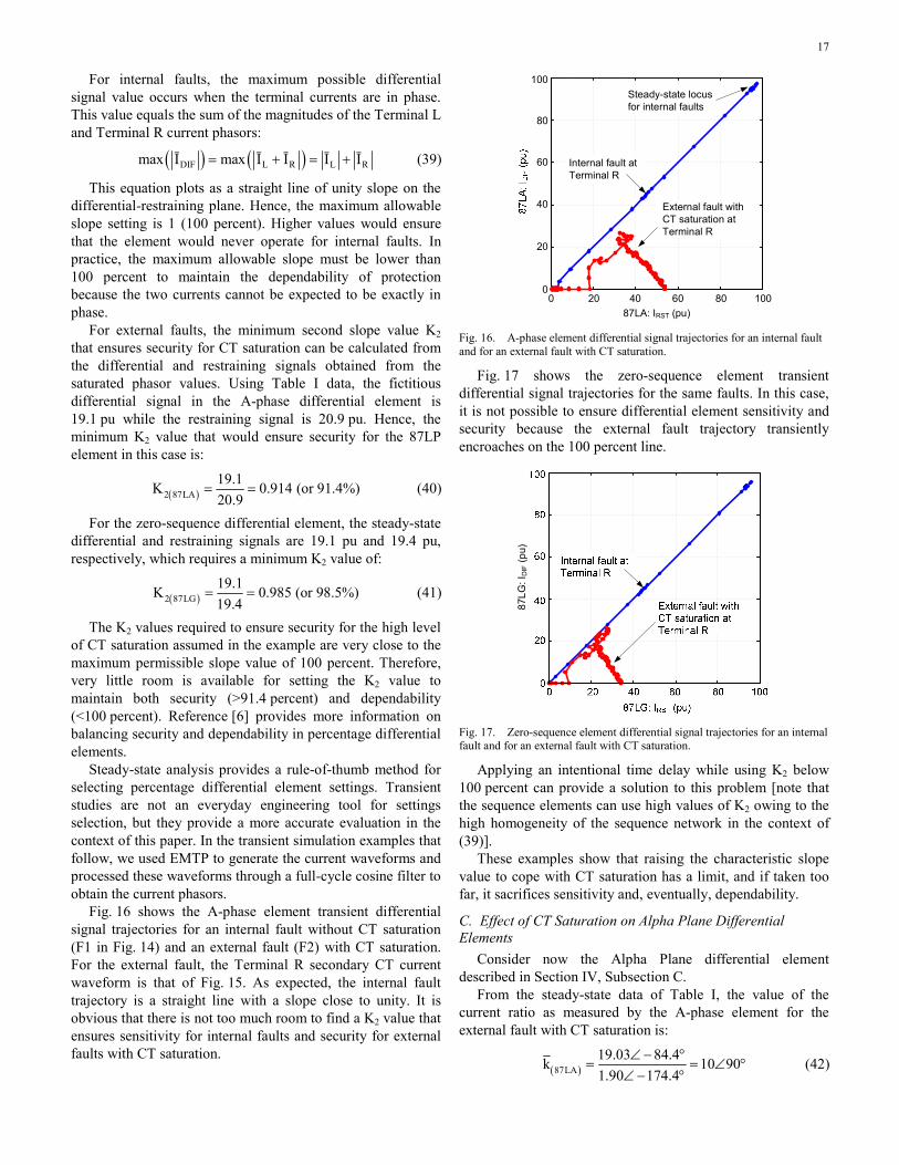
17

For internal faults, the maximum possible differential signal value occurs when the terminal currents are in phase. This value equals the sum of the magnitudes of the Terminal L and Terminal R current phasors:

( ) ( )DIF L R L Rmax Ī max Ī Ī Ī Ī= + = + (39)

This equation plots as a straight line of unity slope on the differential-restraining plane. Hence, the maximum allowable slope setting is 1 (100 percent). Higher values would ensure that the element would never operate for internal faults. In practice, the maximum allowable slope must be lower than 100 percent to maintain the dependability of protection because the two currents cannot be expected to be exactly in phase.

For external faults, the minimum second slope value K2 that ensures security for CT saturation can be calculated from the differential and restraining signals obtained from the saturated phasor values. Using Table I data, the fictitious differential signal in the A-phase differential element is 19.1 pu while the restraining signal is 20.9 pu. Hence, the minimum K2 value that would ensure security for the 87LP element in this case is:

( )2 87LA19.1K 0.914 (or 91.4%)20.9

= = (40)

For the zero-sequence differential element, the steady-state differential and restraining signals are 19.1 pu and 19.4 pu, respectively, which requires a minimum K2 value of:

( )2 87LG19.1K 0.985 (or 98.5%)19.4

= = (41)

The K2 values required to ensure security for the high level of CT saturation assumed in the example are very close to the maximum permissible slope value of 100 percent. Therefore, very little room is available for setting the K2 value to maintain both security (>91.4 percent) and dependability (<100 percent). Reference [6] provides more information on balancing security and dependability in percentage differential elements.

Steady-state analysis provides a rule-of-thumb method for selecting percentage differential element settings. Transient studies are not an everyday engineering tool for settings selection, but they provide a more accurate evaluation in the context of this paper. In the transient simulation examples that follow, we used EMTP to generate the current waveforms and processed these waveforms through a full-cycle cosine filter to obtain the current phasors.

Fig. 16 shows the A-phase element transient differential signal trajectories for an internal fault without CT saturation (F1 in Fig. 14) and an external fault (F2) with CT saturation. For the external fault, the Terminal R secondary CT current waveform is that of Fig. 15. As expected, the internal fault trajectory is a straight line with a slope close to unity. It is obvious that there is not too much room to find a K2 value that ensures sensitivity for internal faults and security for external faults with CT saturation.

0 20 40 60 80 1000

20

40

60

80

100

87LA: IRST (pu)

External fault with CT saturation at Terminal R

Internal fault at Terminal R

Steady-state locus for internal faults

Fig. 16. A-phase element differential signal trajectories for an internal fault and for an external fault with CT saturation.

Fig. 17 shows the zero-sequence element transient differential signal trajectories for the same faults. In this case, it is not possible to ensure differential element sensitivity and security because the external fault trajectory transiently encroaches on the 100 percent line.

87LG

: ID

IF(p

u)

Fig. 17. Zero-sequence element differential signal trajectories for an internal fault and for an external fault with CT saturation.

Applying an intentional time delay while using K2 below 100 percent can provide a solution to this problem [note that the sequence elements can use high values of K2 owing to the high homogeneity of the sequence network in the context of (39)].

These examples show that raising the characteristic slope value to cope with CT saturation has a limit, and if taken too far, it sacrifices sensitivity and, eventually, dependability.

C. Effect of CT Saturation on Alpha Plane Differential Elements

Consider now the Alpha Plane differential element described in Section IV, Subsection C.

From the steady-state data of Table I, the value of the current ratio as measured by the A-phase element for the external fault with CT saturation is:

( )87LA19.03 84.4k 10 901.90 174.4

∠− °= = ∠ °

∠− ° (42)

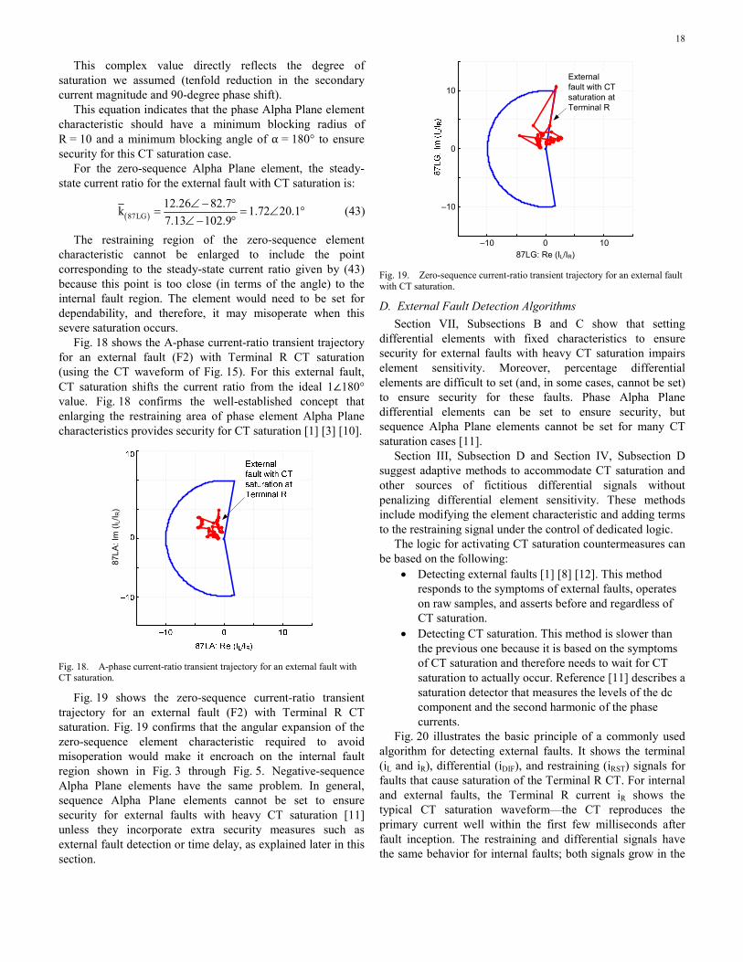
18

This complex value directly reflects the degree of saturation we assumed (tenfold reduction in the secondary current magnitude and 90-degree phase shift).

This equation indicates that the phase Alpha Plane element characteristic should have a minimum blocking radius of R = 10 and a minimum blocking angle of α = 180° to ensure security for this CT saturation case.

For the zero-sequence Alpha Plane element, the steady-state current ratio for the external fault with CT saturation is:

( )87LG12.26 82.7k 1.72 20.17.13 102.9

∠− °= = ∠ °

∠− ° (43)

The restraining region of the zero-sequence element characteristic cannot be enlarged to include the point corresponding to the steady-state current ratio given by (43) because this point is too close (in terms of the angle) to the internal fault region. The element would need to be set for dependability, and therefore, it may misoperate when this severe saturation occurs.

Fig. 18 shows the A-phase current-ratio transient trajectory for an external fault (F2) with Terminal R CT saturation (using the CT waveform of Fig. 15). For this external fault, CT saturation shifts the current ratio from the ideal 1∠180° value. Fig. 18 confirms the well-established concept that enlarging the restraining area of phase element Alpha Plane characteristics provides security for CT saturation [1] [3] [10].

87LA

: Im

(IL/I

R)

Fig. 18. A-phase current-ratio transient trajectory for an external fault with CT saturation.

Fig. 19 shows the zero-sequence current-ratio transient trajectory for an external fault (F2) with Terminal R CT saturation. Fig. 19 confirms that the angular expansion of the zero-sequence element characteristic required to avoid misoperation would make it encroach on the internal fault region shown in Fig. 3 through Fig. 5. Negative-sequence Alpha Plane elements have the same problem. In general, sequence Alpha Plane elements cannot be set to ensure security for external faults with heavy CT saturation [11] unless they incorporate extra security measures such as external fault detection or time delay, as explained later in this section.

–10 0 10

–10

0

10

87LG: Re (IL/IR)

External fault with CT saturation at Terminal R

Fig. 19. Zero-sequence current-ratio transient trajectory for an external fault with CT saturation.

D. External Fault Detection Algorithms Section VII, Subsections B and C show that setting

differential elements with fixed characteristics to ensure security for external faults with heavy CT saturation impairs element sensitivity. Moreover, percentage differential elements are difficult to set (and, in some cases, cannot be set) to ensure security for these faults. Phase Alpha Plane differential elements can be set to ensure security, but sequence Alpha Plane elements cannot be set for many CT saturation cases [11].

Section III, Subsection D and Section IV, Subsection D suggest adaptive methods to accommodate CT saturation and other sources of fictitious differential signals without penalizing differential element sensitivity. These methods include modifying the element characteristic and adding terms to the restraining signal under the control of dedicated logic.

The logic for activating CT saturation countermeasures can be based on the following:

• Detecting external faults [1] [8] [12]. This method responds to the symptoms of external faults, operates on raw samples, and asserts before and regardless of CT saturation.

• Detecting CT saturation. This method is slower than the previous one because it is based on the symptoms of CT saturation and therefore needs to wait for CT saturation to actually occur. Reference [11] describes a saturation detector that measures the levels of the dc component and the second harmonic of the phase currents.

Fig. 20 illustrates the basic principle of a commonly used algorithm for detecting external faults. It shows the terminal (iL and iR), differential (iDIF), and restraining (iRST) signals for faults that cause saturation of the Terminal R CT. For internal and external faults, the Terminal R current iR shows the typical CT saturation waveform—the CT reproduces the primary current well within the first few milliseconds after fault inception. The restraining and differential signals have the same behavior for internal faults; both signals grow in the

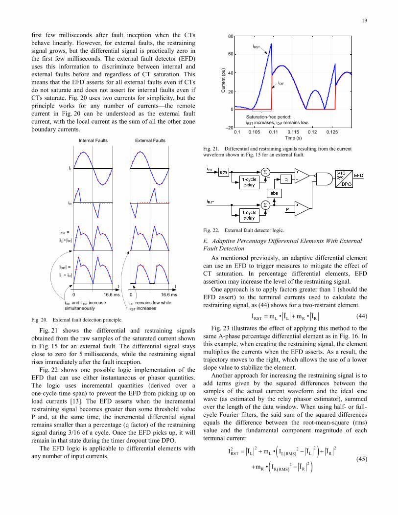
19

first few milliseconds after fault inception when the CTs behave linearly. However, for external faults, the restraining signal grows, but the differential signal is practically zero in the first few milliseconds. The external fault detector (EFD) uses this information to discriminate between internal and external faults before and regardless of CT saturation. This means that the EFD asserts for all external faults even if CTs do not saturate and does not assert for internal faults even if CTs saturate. Fig. 20 uses two currents for simplicity, but the principle works for any number of currents—the remote current in Fig. 20 can be understood as the external fault current, with the local current as the sum of all the other zone boundary currents.

Internal Faults External Faults

iDIF and iRST increase simultaneously

iDIF remains low while iRST increases

iL

iR

|iDIF| =

|iL + iR|

iRST =

|iL|+|iR|

t t

0 16.6 ms0 16.6 ms

Fig. 20. External fault detection principle.

Fig. 21 shows the differential and restraining signals obtained from the raw samples of the saturated current shown in Fig. 15 for an external fault. The differential signal stays close to zero for 5 milliseconds, while the restraining signal rises immediately after the fault inception.

Fig. 22 shows one possible logic implementation of the EFD that can use either instantaneous or phasor quantities. The logic uses incremental quantities (derived over a one-cycle time span) to prevent the EFD from picking up on load currents [13]. The EFD asserts when the incremental restraining signal becomes greater than some threshold value P and, at the same time, the incremental differential signal remains smaller than a percentage (q factor) of the restraining signal during 3/16 of a cycle. Once the EFD picks up, it will remain in that state during the timer dropout time DPO.

The EFD logic is applicable to differential elements with any number of input currents.

0.1 0.105 0.11 0.115 0.12 0.125–20

0

20

40

60

80

Time (s)

Cur

rent

(pu)

Saturation-free period:iRST increases, iDIF remains low.

iDIF

iRST

Fig. 21. Differential and restraining signals resulting from the current waveform shown in Fig. 15 for an external fault.

Σ

Σ

Fig. 22. External fault detector logic.

E. Adaptive Percentage Differential Elements With External Fault Detection

As mentioned previously, an adaptive differential element can use an EFD to trigger measures to mitigate the effect of CT saturation. In percentage differential elements, EFD assertion may increase the level of the restraining signal.

One approach is to apply factors greater than 1 (should the EFD assert) to the terminal currents used to calculate the restraining signal, as (44) shows for a two-restraint element.

RST L L R RI m • Ī m • Ī= + (44)

Fig. 23 illustrates the effect of applying this method to the same A-phase percentage differential element as in Fig. 16. In this example, when creating the restraining signal, the element multiplies the currents when the EFD asserts. As a result, the trajectory moves to the right, which allows the use of a lower slope value to stabilize the element.

Another approach for increasing the restraining signal is to add terms given by the squared differences between the samples of the actual current waveform and the ideal sine wave (as estimated by the relay phasor estimator), summed over the length of the data window. When using half- or full-cycle Fourier filters, the said sum of the squared differences equals the difference between the root-mean-square (rms) value and the fundamental component magnitude of each terminal current:

( )( )

( )( )

2 2 22 2RST L L L RL RMS

22R RR RMS

I Ī m • I Ī Ī

m • I Ī

= + − +

+ − (45)

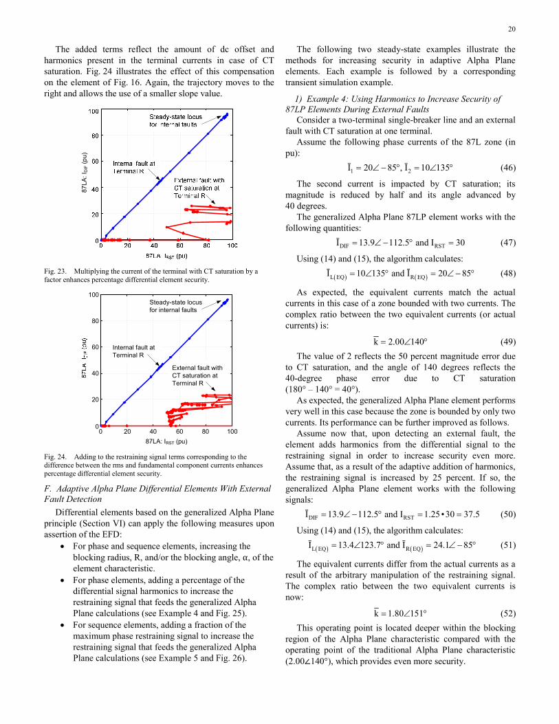
20

The added terms reflect the amount of dc offset and harmonics present in the terminal currents in case of CT saturation. Fig. 24 illustrates the effect of this compensation on the element of Fig. 16. Again, the trajectory moves to the right and allows the use of a smaller slope value.

87LA

: ID

IF(p

u)

Fig. 23. Multiplying the current of the terminal with CT saturation by a factor enhances percentage differential element security.

0 20 40 60 80 1000

20

40

60

80

100

87LA: IRST (pu)

Steady-state locus for internal faults

Internal fault at Terminal R

External fault with CT saturation at Terminal R

Fig. 24. Adding to the restraining signal terms corresponding to the difference between the rms and fundamental component currents enhances percentage differential element security.

F. Adaptive Alpha Plane Differential Elements With External Fault Detection

Differential elements based on the generalized Alpha Plane principle (Section VI) can apply the following measures upon assertion of the EFD:

• For phase and sequence elements, increasing the blocking radius, R, and/or the blocking angle, α, of the element characteristic.

• For phase elements, adding a percentage of the differential signal harmonics to increase the restraining signal that feeds the generalized Alpha Plane calculations (see Example 4 and Fig. 25).

• For sequence elements, adding a fraction of the maximum phase restraining signal to increase the restraining signal that feeds the generalized Alpha Plane calculations (see Example 5 and Fig. 26).

The following two steady-state examples illustrate the methods for increasing security in adaptive Alpha Plane elements. Each example is followed by a corresponding transient simulation example.

1) Example 4: Using Harmonics to Increase Security of 87LP Elements During External Faults

Consider a two-terminal single-breaker line and an external fault with CT saturation at one terminal.

Assume the following phase currents of the 87L zone (in pu): 1 2Ī 20 85 , Ī 10 135= ∠− ° = ∠ ° (46)

The second current is impacted by CT saturation; its magnitude is reduced by half and its angle advanced by 40 degrees.

The generalized Alpha Plane 87LP element works with the following quantities: DIF RSTĪ 13.9 112.5 and I 30= ∠− ° = (47)

Using (14) and (15), the algorithm calculates: ( ) ( )L EQ R EQĪ 10 135 and Ī 20 85= ∠ ° = ∠− ° (48)

As expected, the equivalent currents match the actual currents in this case of a zone bounded with two currents. The complex ratio between the two equivalent currents (or actual currents) is:

k 2.00 140= ∠ ° (49) The value of 2 reflects the 50 percent magnitude error due

to CT saturation, and the angle of 140 degrees reflects the 40-degree phase error due to CT saturation (180° – 140° = 40°).

As expected, the generalized Alpha Plane element performs very well in this case because the zone is bounded by only two currents. Its performance can be further improved as follows.

Assume now that, upon detecting an external fault, the element adds harmonics from the differential signal to the restraining signal in order to increase security even more. Assume that, as a result of the adaptive addition of harmonics, the restraining signal is increased by 25 percent. If so, the generalized Alpha Plane element works with the following signals: DIF RSTĪ 13.9 112.5 and I 1.25 •30 37.5= ∠− ° = = (50)

Using (14) and (15), the algorithm calculates: ( ) ( )L EQ R EQĪ 13.4 123.7 and Ī 24.1 85= ∠ ° = ∠− ° (51)

The equivalent currents differ from the actual currents as a result of the arbitrary manipulation of the restraining signal. The complex ratio between the two equivalent currents is now:

k 1.80 151= ∠ ° (52) This operating point is located deeper within the blocking

region of the Alpha Plane characteristic compared with the operating point of the traditional Alpha Plane characteristic (2.00∠140°), which provides even more security.

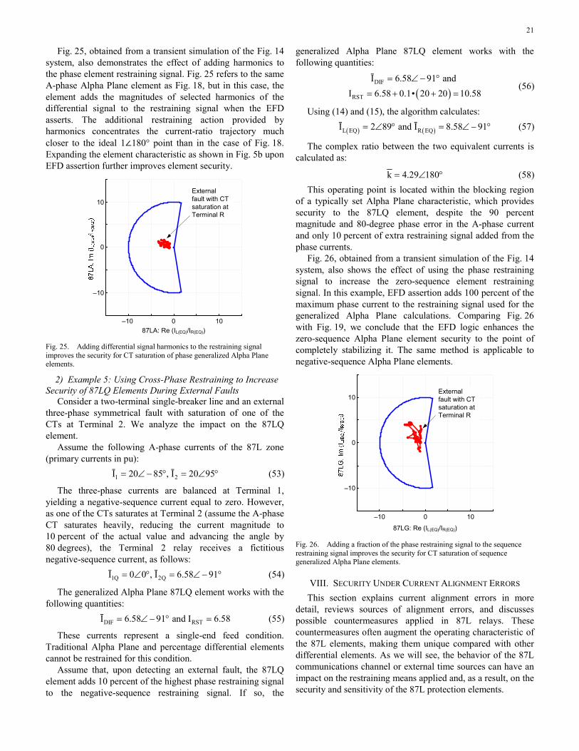
21

Fig. 25, obtained from a transient simulation of the Fig. 14 system, also demonstrates the effect of adding harmonics to the phase element restraining signal. Fig. 25 refers to the same A-phase Alpha Plane element as Fig. 18, but in this case, the element adds the magnitudes of selected harmonics of the differential signal to the restraining signal when the EFD asserts. The additional restraining action provided by harmonics concentrates the current-ratio trajectory much closer to the ideal 1∠180° point than in the case of Fig. 18. Expanding the element characteristic as shown in Fig. 5b upon EFD assertion further improves element security.

–10 0 10

–10

0

10

87LA: Re (IL(EQ)/IR(EQ))

External fault with CT saturation at Terminal R

Fig. 25. Adding differential signal harmonics to the restraining signal improves the security for CT saturation of phase generalized Alpha Plane elements.

2) Example 5: Using Cross-Phase Restraining to Increase Security of 87LQ Elements During External Faults

Consider a two-terminal single-breaker line and an external three-phase symmetrical fault with saturation of one of the CTs at Terminal 2. We analyze the impact on the 87LQ element.

Assume the following A-phase currents of the 87L zone (primary currents in pu): 1 2Ī 20 85 , Ī 20 95= ∠− ° = ∠ ° (53)

The three-phase currents are balanced at Terminal 1, yielding a negative-sequence current equal to zero. However, as one of the CTs saturates at Terminal 2 (assume the A-phase CT saturates heavily, reducing the current magnitude to 10 percent of the actual value and advancing the angle by 80 degrees), the Terminal 2 relay receives a fictitious negative-sequence current, as follows: 1Q 2QĪ 0 0 , Ī 6.58 91= ∠ ° = ∠− ° (54)

The generalized Alpha Plane 87LQ element works with the following quantities: DIF RSTĪ 6.58 91 and I 6.58= ∠− ° = (55)

These currents represent a single-end feed condition. Traditional Alpha Plane and percentage differential elements cannot be restrained for this condition.

Assume that, upon detecting an external fault, the 87LQ element adds 10 percent of the highest phase restraining signal to the negative-sequence restraining signal. If so, the

generalized Alpha Plane 87LQ element works with the following quantities:

( )

DIF

RST

Ī 6.58 91 and I 6.58 0.1• 20 20 10.58

= ∠− °

= + + = (56)

Using (14) and (15), the algorithm calculates: ( ) ( )L EQ R EQĪ 2 89 and Ī 8.58 91= ∠ ° = ∠− ° (57)

The complex ratio between the two equivalent currents is calculated as:

k 4.29 180= ∠ ° (58) This operating point is located within the blocking region

of a typically set Alpha Plane characteristic, which provides security to the 87LQ element, despite the 90 percent magnitude and 80-degree phase error in the A-phase current and only 10 percent of extra restraining signal added from the phase currents.

Fig. 26, obtained from a transient simulation of the Fig. 14 system, also shows the effect of using the phase restraining signal to increase the zero-sequence element restraining signal. In this example, EFD assertion adds 100 percent of the maximum phase current to the restraining signal used for the generalized Alpha Plane calculations. Comparing Fig. 26 with Fig. 19, we conclude that the EFD logic enhances the zero-sequence Alpha Plane element security to the point of completely stabilizing it. The same method is applicable to negative-sequence Alpha Plane elements.

–10 0 10

–10

0

10

87LG: Re (IL(EQ)/IR(EQ))

External fault with CT saturation at Terminal R

Fig. 26. Adding a fraction of the phase restraining signal to the sequence restraining signal improves the security for CT saturation of sequence generalized Alpha Plane elements.

VIII. SECURITY UNDER CURRENT ALIGNMENT ERRORS This section explains current alignment errors in more

detail, reviews sources of alignment errors, and discusses possible countermeasures applied in 87L relays. These countermeasures often augment the operating characteristic of the 87L elements, making them unique compared with other differential elements. As we will see, the behavior of the 87L communications channel or external time sources can have an impact on the restraining means applied and, as a result, on the security and sensitivity of the 87L protection elements.

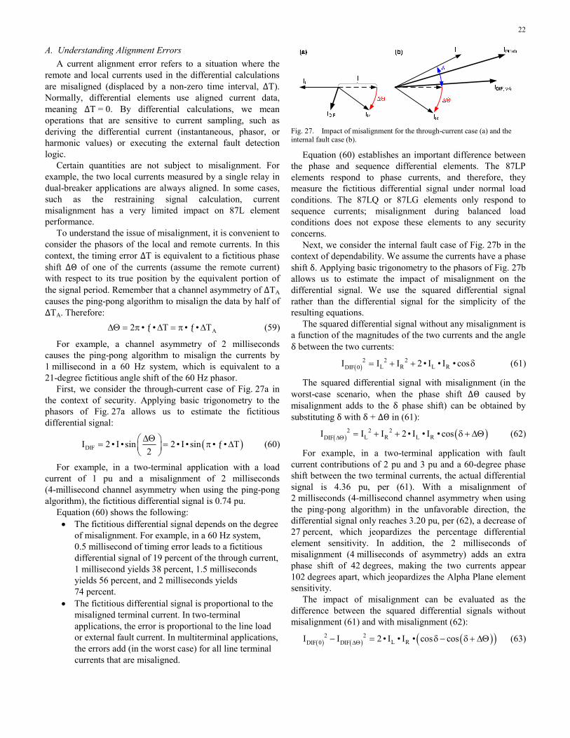
22

A. Understanding Alignment Errors A current alignment error refers to a situation where the

remote and local currents used in the differential calculations are misaligned (displaced by a non-zero time interval, ΔT). Normally, differential elements use aligned current data, meaning ΔT = 0. By differential calculations, we mean operations that are sensitive to current sampling, such as deriving the differential current (instantaneous, phasor, or harmonic values) or executing the external fault detection logic.

Certain quantities are not subject to misalignment. For example, the two local currents measured by a single relay in dual-breaker applications are always aligned. In some cases, such as the restraining signal calculation, current misalignment has a very limited impact on 87L element performance.

To understand the issue of misalignment, it is convenient to consider the phasors of the local and remote currents. In this context, the timing error ΔT is equivalent to a fictitious phase shift ΔΘ of one of the currents (assume the remote current) with respect to its true position by the equivalent portion of the signal period. Remember that a channel asymmetry of ΔTA causes the ping-pong algorithm to misalign the data by half of ΔTA. Therefore: A2 • • • •ΔΘ = π ƒ ΔΤ = π ƒ ΔΤ (59)

For example, a channel asymmetry of 2 milliseconds causes the ping-pong algorithm to misalign the currents by 1 millisecond in a 60 Hz system, which is equivalent to a 21-degree fictitious angle shift of the 60 Hz phasor.

First, we consider the through-current case of Fig. 27a in the context of security. Applying basic trigonometry to the phasors of Fig. 27a allows us to estimate the fictitious differential signal:

( )DIFI 2 • I • sin 2 • I • sin • •2ΔΘ⎛ ⎞= = π ƒ ΔΤ⎜ ⎟

⎝ ⎠ (60)

For example, in a two-terminal application with a load current of 1 pu and a misalignment of 2 milliseconds (4-millisecond channel asymmetry when using the ping-pong algorithm), the fictitious differential signal is 0.74 pu.

Equation (60) shows the following: • The fictitious differential signal depends on the degree

of misalignment. For example, in a 60 Hz system, 0.5 millisecond of timing error leads to a fictitious differential signal of 19 percent of the through current, 1 millisecond yields 38 percent, 1.5 milliseconds yields 56 percent, and 2 milliseconds yields 74 percent.

• The fictitious differential signal is proportional to the misaligned terminal current. In two-terminal applications, the error is proportional to the line load or external fault current. In multiterminal applications, the errors add (in the worst case) for all line terminal currents that are misaligned.

Fig. 27. Impact of misalignment for the through-current case (a) and the internal fault case (b).

Equation (60) establishes an important difference between the phase and sequence differential elements. The 87LP elements respond to phase currents, and therefore, they measure the fictitious differential signal under normal load conditions. The 87LQ or 87LG elements only respond to sequence currents; misalignment during balanced load conditions does not expose these elements to any security concerns.

Next, we consider the internal fault case of Fig. 27b in the context of dependability. We assume the currents have a phase shift δ. Applying basic trigonometry to the phasors of Fig. 27b allows us to estimate the impact of misalignment on the differential signal. We use the squared differential signal rather than the differential signal for the simplicity of the resulting equations.

The squared differential signal without any misalignment is a function of the magnitudes of the two currents and the angle δ between the two currents:

( )2 2 2

L R L RDIF 0I I I 2 • I • I • cos= + + δ (61)

The squared differential signal with misalignment (in the worst-case scenario, when the phase shift ΔΘ caused by misalignment adds to the δ phase shift) can be obtained by substituting δ with δ + ΔΘ in (61):

( ) ( )2 2 2L R L RDIFI I I 2 • I • I • cosΔΘ = + + δ + ΔΘ (62)

For example, in a two-terminal application with fault current contributions of 2 pu and 3 pu and a 60-degree phase shift between the two terminal currents, the actual differential signal is 4.36 pu, per (61). With a misalignment of 2 milliseconds (4-millisecond channel asymmetry when using the ping-pong algorithm) in the unfavorable direction, the differential signal only reaches 3.20 pu, per (62), a decrease of 27 percent, which jeopardizes the percentage differential element sensitivity. In addition, the 2 milliseconds of misalignment (4 milliseconds of asymmetry) adds an extra phase shift of 42 degrees, making the two currents appear 102 degrees apart, which jeopardizes the Alpha Plane element sensitivity.

The impact of misalignment can be evaluated as the difference between the squared differential signals without misalignment (61) and with misalignment (62):

( ) ( ) ( )( )2 2L RDIF 0 DIFI I 2 • I • I • cos cosΔΘ− = δ − δ + ΔΘ (63)

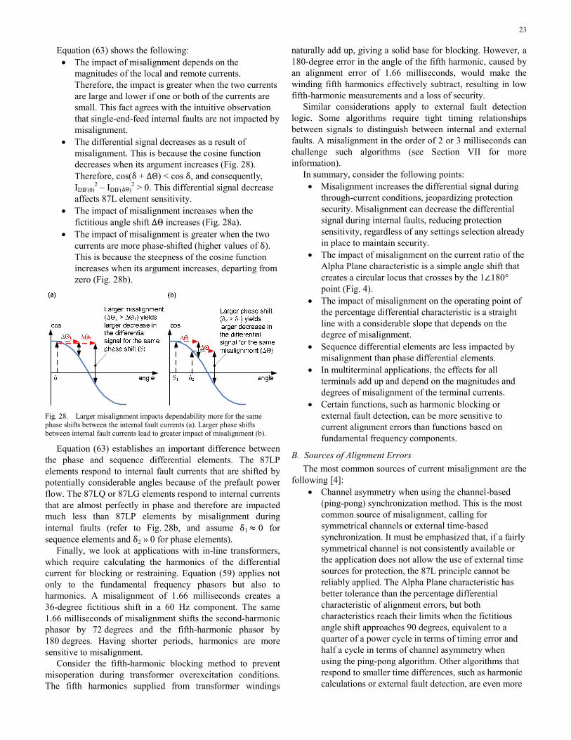
23

Equation (63) shows the following: • The impact of misalignment depends on the

magnitudes of the local and remote currents. Therefore, the impact is greater when the two currents are large and lower if one or both of the currents are small. This fact agrees with the intuitive observation that single-end-feed internal faults are not impacted by misalignment.

• The differential signal decreases as a result of misalignment. This is because the cosine function decreases when its argument increases (Fig. 28). Therefore, cos(δ + ΔΘ) < cos δ, and consequently, IDIF(0)

2 – IDIF(ΔΘ)2 > 0. This differential signal decrease

affects 87L element sensitivity. • The impact of misalignment increases when the

fictitious angle shift ΔΘ increases (Fig. 28a). • The impact of misalignment is greater when the two

currents are more phase-shifted (higher values of δ). This is because the steepness of the cosine function increases when its argument increases, departing from zero (Fig. 28b).

Fig. 28. Larger misalignment impacts dependability more for the same phase shifts between the internal fault currents (a). Larger phase shifts between internal fault currents lead to greater impact of misalignment (b).

Equation (63) establishes an important difference between the phase and sequence differential elements. The 87LP elements respond to internal fault currents that are shifted by potentially considerable angles because of the prefault power flow. The 87LQ or 87LG elements respond to internal currents that are almost perfectly in phase and therefore are impacted much less than 87LP elements by misalignment during internal faults (refer to Fig. 28b, and assume δ1 ≈ 0 for sequence elements and δ2 » 0 for phase elements).

Finally, we look at applications with in-line transformers, which require calculating the harmonics of the differential current for blocking or restraining. Equation (59) applies not only to the fundamental frequency phasors but also to harmonics. A misalignment of 1.66 milliseconds creates a 36-degree fictitious shift in a 60 Hz component. The same 1.66 milliseconds of misalignment shifts the second-harmonic phasor by 72 degrees and the fifth-harmonic phasor by 180 degrees. Having shorter periods, harmonics are more sensitive to misalignment.

Consider the fifth-harmonic blocking method to prevent misoperation during transformer overexcitation conditions. The fifth harmonics supplied from transformer windings

naturally add up, giving a solid base for blocking. However, a 180-degree error in the angle of the fifth harmonic, caused by an alignment error of 1.66 milliseconds, would make the winding fifth harmonics effectively subtract, resulting in low fifth-harmonic measurements and a loss of security.

Similar considerations apply to external fault detection logic. Some algorithms require tight timing relationships between signals to distinguish between internal and external faults. A misalignment in the order of 2 or 3 milliseconds can challenge such algorithms (see Section VII for more information).

In summary, consider the following points: • Misalignment increases the differential signal during

through-current conditions, jeopardizing protection security. Misalignment can decrease the differential signal during internal faults, reducing protection sensitivity, regardless of any settings selection already in place to maintain security.

• The impact of misalignment on the current ratio of the Alpha Plane characteristic is a simple angle shift that creates a circular locus that crosses by the 1∠180° point (Fig. 4).

• The impact of misalignment on the operating point of the percentage differential characteristic is a straight line with a considerable slope that depends on the degree of misalignment.

• Sequence differential elements are less impacted by misalignment than phase differential elements.

• In multiterminal applications, the effects for all terminals add up and depend on the magnitudes and degrees of misalignment of the terminal currents.

• Certain functions, such as harmonic blocking or external fault detection, can be more sensitive to current alignment errors than functions based on fundamental frequency components.

B. Sources of Alignment Errors The most common sources of current misalignment are the

following [4]: • Channel asymmetry when using the channel-based

(ping-pong) synchronization method. This is the most common source of misalignment, calling for symmetrical channels or external time-based synchronization. It must be emphasized that, if a fairly symmetrical channel is not consistently available or the application does not allow the use of external time sources for protection, the 87L principle cannot be reliably applied. The Alpha Plane characteristic has better tolerance than the percentage differential characteristic of alignment errors, but both characteristics reach their limits when the fictitious angle shift approaches 90 degrees, equivalent to a quarter of a power cycle in terms of timing error and half a cycle in terms of channel asymmetry when using the ping-pong algorithm. Other algorithms that respond to smaller time differences, such as harmonic calculations or external fault detection, are even more

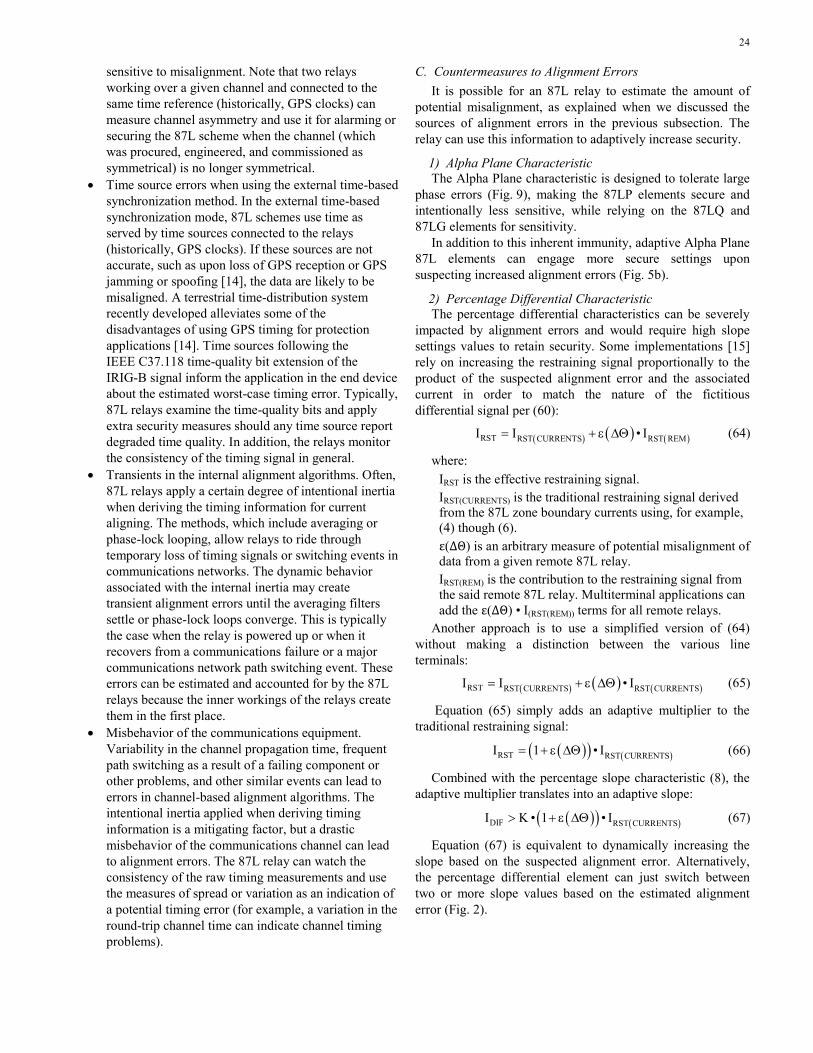
24

sensitive to misalignment. Note that two relays working over a given channel and connected to the same time reference (historically, GPS clocks) can measure channel asymmetry and use it for alarming or securing the 87L scheme when the channel (which was procured, engineered, and commissioned as symmetrical) is no longer symmetrical.

• Time source errors when using the external time-based synchronization method. In the external time-based synchronization mode, 87L schemes use time as served by time sources connected to the relays (historically, GPS clocks). If these sources are not accurate, such as upon loss of GPS reception or GPS jamming or spoofing [14], the data are likely to be misaligned. A terrestrial time-distribution system recently developed alleviates some of the disadvantages of using GPS timing for protection applications [14]. Time sources following the IEEE C37.118 time-quality bit extension of the IRIG-B signal inform the application in the end device about the estimated worst-case timing error. Typically, 87L relays examine the time-quality bits and apply extra security measures should any time source report degraded time quality. In addition, the relays monitor the consistency of the timing signal in general.

• Transients in the internal alignment algorithms. Often, 87L relays apply a certain degree of intentional inertia when deriving the timing information for current aligning. The methods, which include averaging or phase-lock looping, allow relays to ride through temporary loss of timing signals or switching events in communications networks. The dynamic behavior associated with the internal inertia may create transient alignment errors until the averaging filters settle or phase-lock loops converge. This is typically the case when the relay is powered up or when it recovers from a communications failure or a major communications network path switching event. These errors can be estimated and accounted for by the 87L relays because the inner workings of the relays create them in the first place.

• Misbehavior of the communications equipment. Variability in the channel propagation time, frequent path switching as a result of a failing component or other problems, and other similar events can lead to errors in channel-based alignment algorithms. The intentional inertia applied when deriving timing information is a mitigating factor, but a drastic misbehavior of the communications channel can lead to alignment errors. The 87L relay can watch the consistency of the raw timing measurements and use the measures of spread or variation as an indication of a potential timing error (for example, a variation in the round-trip channel time can indicate channel timing problems).

C. Countermeasures to Alignment Errors It is possible for an 87L relay to estimate the amount of

potential misalignment, as explained when we discussed the sources of alignment errors in the previous subsection. The relay can use this information to adaptively increase security.

1) Alpha Plane Characteristic The Alpha Plane characteristic is designed to tolerate large

phase errors (Fig. 9), making the 87LP elements secure and intentionally less sensitive, while relying on the 87LQ and 87LG elements for sensitivity.

In addition to this inherent immunity, adaptive Alpha Plane 87L elements can engage more secure settings upon suspecting increased alignment errors (Fig. 5b).

2) Percentage Differential Characteristic The percentage differential characteristics can be severely

impacted by alignment errors and would require high slope settings values to retain security. Some implementations [15] rely on increasing the restraining signal proportionally to the product of the suspected alignment error and the associated current in order to match the nature of the fictitious differential signal per (60):

( ) ( ) ( )RST RST CURRENTS RST REMI I • I= + ε ΔΘ (64)

where: IRST is the effective restraining signal. IRST(CURRENTS) is the traditional restraining signal derived from the 87L zone boundary currents using, for example, (4) though (6). ε(ΔΘ) is an arbitrary measure of potential misalignment of data from a given remote 87L relay. IRST(REM) is the contribution to the restraining signal from the said remote 87L relay. Multiterminal applications can add the ε(ΔΘ) • I(RST(REM)) terms for all remote relays.

Another approach is to use a simplified version of (64) without making a distinction between the various line terminals:

( ) ( ) ( )RST RST CURRENTS RST CURRENTSI I • I= + ε ΔΘ (65)

Equation (65) simply adds an adaptive multiplier to the traditional restraining signal:

( )( ) ( )RST RST CURRENTSI 1 • I= + ε ΔΘ (66)

Combined with the percentage slope characteristic (8), the adaptive multiplier translates into an adaptive slope:

( )( ) ( )DIF RST CURRENTSI K • 1 • I> + ε ΔΘ (67)

Equation (67) is equivalent to dynamically increasing the slope based on the suspected alignment error. Alternatively, the percentage differential element can just switch between two or more slope values based on the estimated alignment error (Fig. 2).

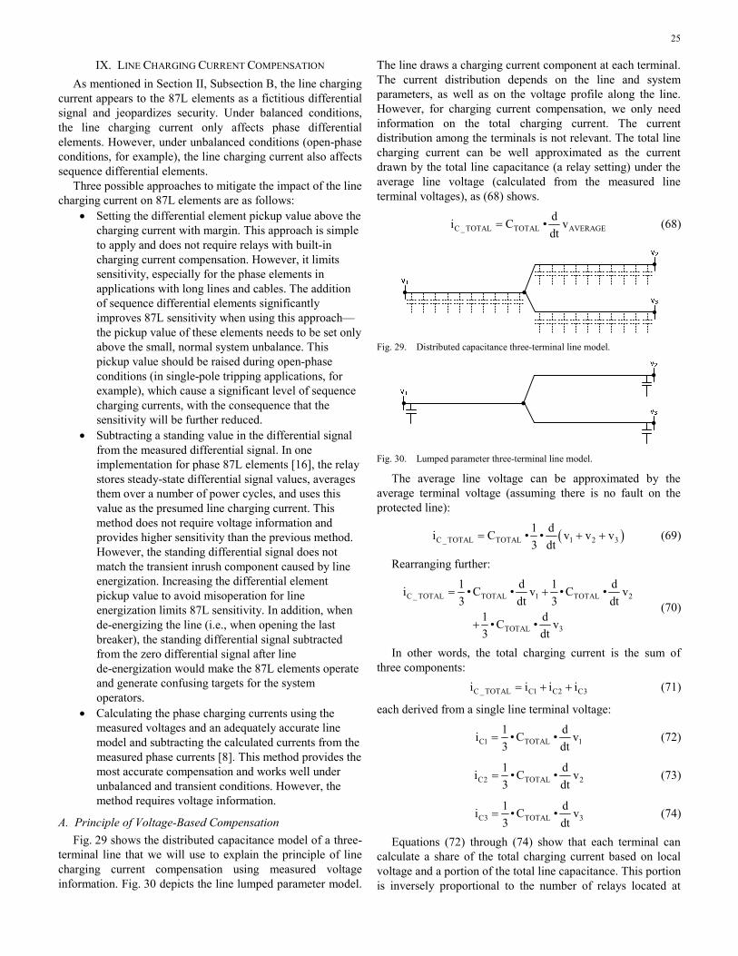
25

IX. LINE CHARGING CURRENT COMPENSATION As mentioned in Section II, Subsection B, the line charging

current appears to the 87L elements as a fictitious differential signal and jeopardizes security. Under balanced conditions, the line charging current only affects phase differential elements. However, under unbalanced conditions (open-phase conditions, for example), the line charging current also affects sequence differential elements.

Three possible approaches to mitigate the impact of the line charging current on 87L elements are as follows:

• Setting the differential element pickup value above the charging current with margin. This approach is simple to apply and does not require relays with built-in charging current compensation. However, it limits sensitivity, especially for the phase elements in applications with long lines and cables. The addition of sequence differential elements significantly improves 87L sensitivity when using this approach—the pickup value of these elements needs to be set only above the small, normal system unbalance. This pickup value should be raised during open-phase conditions (in single-pole tripping applications, for example), which cause a significant level of sequence charging currents, with the consequence that the sensitivity will be further reduced.

• Subtracting a standing value in the differential signal from the measured differential signal. In one implementation for phase 87L elements [16], the relay stores steady-state differential signal values, averages them over a number of power cycles, and uses this value as the presumed line charging current. This method does not require voltage information and provides higher sensitivity than the previous method. However, the standing differential signal does not match the transient inrush component caused by line energization. Increasing the differential element pickup value to avoid misoperation for line energization limits 87L sensitivity. In addition, when de-energizing the line (i.e., when opening the last breaker), the standing differential signal subtracted from the zero differential signal after line de-energization would make the 87L elements operate and generate confusing targets for the system operators.

• Calculating the phase charging currents using the measured voltages and an adequately accurate line model and subtracting the calculated currents from the measured phase currents [8]. This method provides the most accurate compensation and works well under unbalanced and transient conditions. However, the method requires voltage information.

A. Principle of Voltage-Based Compensation Fig. 29 shows the distributed capacitance model of a three-

terminal line that we will use to explain the principle of line charging current compensation using measured voltage information. Fig. 30 depicts the line lumped parameter model.

The line draws a charging current component at each terminal. The current distribution depends on the line and system parameters, as well as on the voltage profile along the line. However, for charging current compensation, we only need information on the total charging current. The current distribution among the terminals is not relevant. The total line charging current can be well approximated as the current drawn by the total line capacitance (a relay setting) under the average line voltage (calculated from the measured line terminal voltages), as (68) shows.

C _ TOTAL TOTAL AVERAGEdi C • vdt

= (68)

Fig. 29. Distributed capacitance three-terminal line model.

Fig. 30. Lumped parameter three-terminal line model.

The average line voltage can be approximated by the average terminal voltage (assuming there is no fault on the protected line):

( )C _ TOTAL TOTAL 1 2 31 di C • • v v v3 dt

= + + (69)

Rearranging further:

C _ TOTAL TOTAL 1 TOTAL 2

TOTAL 3

1 d 1 di • C • v • C • v3 dt 3 dt

1 d• C • v3 dt

= +

+ (70)

In other words, the total charging current is the sum of three components: C _ TOTAL C1 C2 C3i i i i= + + (71)

each derived from a single line terminal voltage:

C1 TOTAL 11 di • C • v3 dt

= (72)

C2 TOTAL 21 di • C • v3 dt

= (73)

C3 TOTAL 31 di • C • v3 dt

= (74)

Equations (72) through (74) show that each terminal can calculate a share of the total charging current based on local voltage and a portion of the total line capacitance. This portion is inversely proportional to the number of relays located at

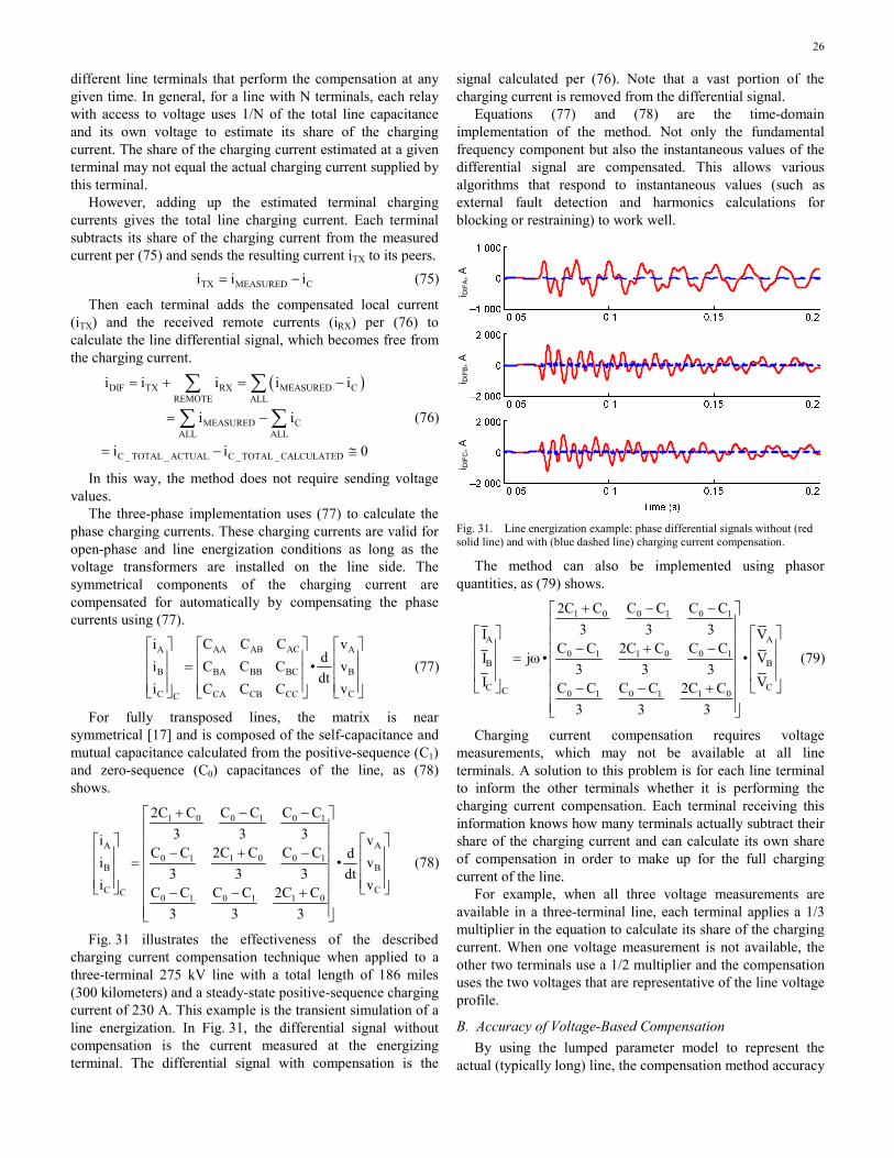
26

different line terminals that perform the compensation at any given time. In general, for a line with N terminals, each relay with access to voltage uses 1/N of the total line capacitance and its own voltage to estimate its share of the charging current. The share of the charging current estimated at a given terminal may not equal the actual charging current supplied by this terminal.

However, adding up the estimated terminal charging currents gives the total line charging current. Each terminal subtracts its share of the charging current from the measured current per (75) and sends the resulting current iTX to its peers. TX MEASURED Ci i i= − (75)

Then each terminal adds the compensated local current (iTX) and the received remote currents (iRX) per (76) to calculate the line differential signal, which becomes free from the charging current.

( )DIF TX RX MEASURED CREMOTE ALL

MEASURED CALL ALL

C _ TOTAL _ ACTUAL C _ TOTAL _ CALCULATED

i i i i i

i i

i i 0

= + = −

= −

= − ≅

∑ ∑

∑ ∑ (76)

In this way, the method does not require sending voltage values.

The three-phase implementation uses (77) to calculate the phase charging currents. These charging currents are valid for open-phase and line energization conditions as long as the voltage transformers are installed on the line side. The symmetrical components of the charging current are compensated for automatically by compensating the phase currents using (77).

AA AB ACA A

B BA BB BC B

C CCA CB CCC

C C Ci vdi C C C • vdt

i vC C C

⎡ ⎤⎡ ⎤ ⎡ ⎤⎢ ⎥⎢ ⎥ ⎢ ⎥= ⎢ ⎥⎢ ⎥ ⎢ ⎥⎢ ⎥⎢ ⎥ ⎢ ⎥⎣ ⎦ ⎣ ⎦⎣ ⎦

(77)

For fully transposed lines, the matrix is near symmetrical [17] and is composed of the self-capacitance and mutual capacitance calculated from the positive-sequence (C1) and zero-sequence (C0) capacitances of the line, as (78) shows.

1 0 0 1 0 1

A A0 1 1 0 0 1

B B

C CC 0 1 0 1 1 0

2C C C C C C

3 3 3i vC C 2C C C C di • v

3 3 3 dti vC C C C 2C C

3 3 3

+ − −⎡ ⎤⎢ ⎥

⎡ ⎤ ⎡ ⎤⎢ ⎥− + −⎢ ⎥ ⎢ ⎥⎢ ⎥=⎢ ⎥ ⎢ ⎥⎢ ⎥

⎢ ⎥ ⎢ ⎥⎢ ⎥⎣ ⎦ ⎣ ⎦− − +⎢ ⎥⎢ ⎥⎣ ⎦

(78)

Fig. 31 illustrates the effectiveness of the described charging current compensation technique when applied to a three-terminal 275 kV line with a total length of 186 miles (300 kilometers) and a steady-state positive-sequence charging current of 230 A. This example is the transient simulation of a line energization. In Fig. 31, the differential signal without compensation is the current measured at the energizing terminal. The differential signal with compensation is the

signal calculated per (76). Note that a vast portion of the charging current is removed from the differential signal.

Equations (77) and (78) are the time-domain implementation of the method. Not only the fundamental frequency component but also the instantaneous values of the differential signal are compensated. This allows various algorithms that respond to instantaneous values (such as external fault detection and harmonics calculations for blocking or restraining) to work well.

i DIF

A, A

i DIF

B, A

i DIF

C, A

Fig. 31. Line energization example: phase differential signals without (red solid line) and with (blue dashed line) charging current compensation.

The method can also be implemented using phasor quantities, as (79) shows.

1 0 0 1 0 1

A A0 1 1 0 0 1

B B

C CC 0 1 0 1 1 0

2C C C C C C

3 3 3I VC C 2C C C C

I j • • V3 3 3

I VC C C C 2C C

3 3 3

+ − −⎡ ⎤⎢ ⎥

⎡ ⎤ ⎡ ⎤⎢ ⎥⎢ ⎥ ⎢ ⎥− + −⎢ ⎥= ω⎢ ⎥ ⎢ ⎥⎢ ⎥⎢ ⎥ ⎢ ⎥⎢ ⎥⎣ ⎦ ⎣ ⎦− − +⎢ ⎥

⎢ ⎥⎣ ⎦

(79)

Charging current compensation requires voltage measurements, which may not be available at all line terminals. A solution to this problem is for each line terminal to inform the other terminals whether it is performing the charging current compensation. Each terminal receiving this information knows how many terminals actually subtract their share of the charging current and can calculate its own share of compensation in order to make up for the full charging current of the line.

For example, when all three voltage measurements are available in a three-terminal line, each terminal applies a 1/3 multiplier in the equation to calculate its share of the charging current. When one voltage measurement is not available, the other two terminals use a 1/2 multiplier and the compensation uses the two voltages that are representative of the line voltage profile.

B. Accuracy of Voltage-Based Compensation By using the lumped parameter model to represent the

actual (typically long) line, the compensation method accuracy

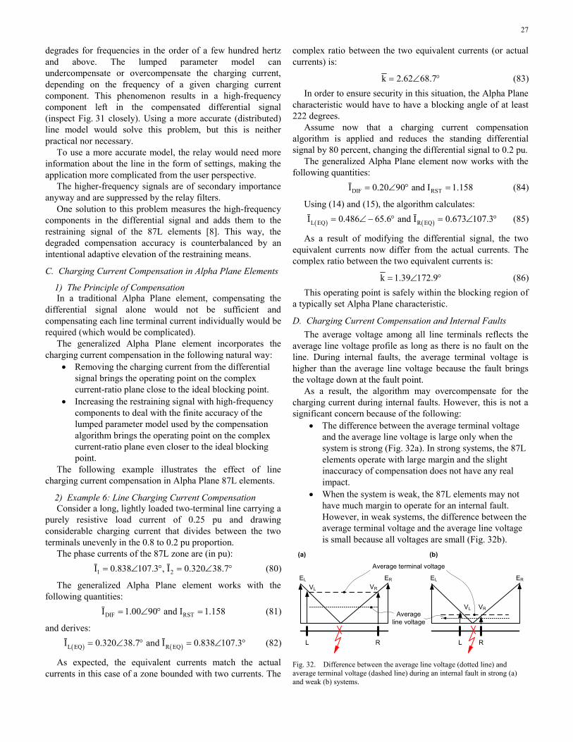
27

degrades for frequencies in the order of a few hundred hertz and above. The lumped parameter model can undercompensate or overcompensate the charging current, depending on the frequency of a given charging current component. This phenomenon results in a high-frequency component left in the compensated differential signal (inspect Fig. 31 closely). Using a more accurate (distributed) line model would solve this problem, but this is neither practical nor necessary.

To use a more accurate model, the relay would need more information about the line in the form of settings, making the application more complicated from the user perspective.

The higher-frequency signals are of secondary importance anyway and are suppressed by the relay filters.

One solution to this problem measures the high-frequency components in the differential signal and adds them to the restraining signal of the 87L elements [8]. This way, the degraded compensation accuracy is counterbalanced by an intentional adaptive elevation of the restraining means.

C. Charging Current Compensation in Alpha Plane Elements

1) The Principle of Compensation In a traditional Alpha Plane element, compensating the

differential signal alone would not be sufficient and compensating each line terminal current individually would be required (which would be complicated).

The generalized Alpha Plane element incorporates the charging current compensation in the following natural way:

• Removing the charging current from the differential signal brings the operating point on the complex current-ratio plane close to the ideal blocking point.

• Increasing the restraining signal with high-frequency components to deal with the finite accuracy of the lumped parameter model used by the compensation algorithm brings the operating point on the complex current-ratio plane even closer to the ideal blocking point.

The following example illustrates the effect of line charging current compensation in Alpha Plane 87L elements.

2) Example 6: Line Charging Current Compensation Consider a long, lightly loaded two-terminal line carrying a

purely resistive load current of 0.25 pu and drawing considerable charging current that divides between the two terminals unevenly in the 0.8 to 0.2 pu proportion.

The phase currents of the 87L zone are (in pu): 1 2Ī 0.838 107.3 , Ī 0.320 38.7= ∠ ° = ∠ ° (80)

The generalized Alpha Plane element works with the following quantities: DIF RSTĪ 1.00 90 and I 1.158= ∠ ° = (81)

and derives: ( ) ( )L EQ R EQĪ 0.320 38.7 and Ī 0.838 107.3= ∠ ° = ∠ ° (82)

As expected, the equivalent currents match the actual currents in this case of a zone bounded with two currents. The

complex ratio between the two equivalent currents (or actual currents) is:

k 2.62 68.7= ∠ ° (83) In order to ensure security in this situation, the Alpha Plane

characteristic would have to have a blocking angle of at least 222 degrees.

Assume now that a charging current compensation algorithm is applied and reduces the standing differential signal by 80 percent, changing the differential signal to 0.2 pu.

The generalized Alpha Plane element now works with the following quantities: DIF RSTĪ 0.20 90 and I 1.158= ∠ ° = (84)

Using (14) and (15), the algorithm calculates: ( ) ( )L EQ R EQĪ 0.486 65.6 and Ī 0.673 107.3= ∠− ° = ∠ ° (85)

As a result of modifying the differential signal, the two equivalent currents now differ from the actual currents. The complex ratio between the two equivalent currents is:

k 1.39 172.9= ∠ ° (86) This operating point is safely within the blocking region of

a typically set Alpha Plane characteristic.

D. Charging Current Compensation and Internal Faults The average voltage among all line terminals reflects the

average line voltage profile as long as there is no fault on the line. During internal faults, the average terminal voltage is higher than the average line voltage because the fault brings the voltage down at the fault point.

As a result, the algorithm may overcompensate for the charging current during internal faults. However, this is not a significant concern because of the following:

• The difference between the average terminal voltage and the average line voltage is large only when the system is strong (Fig. 32a). In strong systems, the 87L elements operate with large margin and the slight inaccuracy of compensation does not have any real impact.

• When the system is weak, the 87L elements may not have much margin to operate for an internal fault. However, in weak systems, the difference between the average terminal voltage and the average line voltage is small because all voltages are small (Fig. 32b).

(a)

ER

VRVL

EL

L R

(b)

ER

VRVL

EL

Average line voltage

L R

Average terminal voltage

Fig. 32. Difference between the average line voltage (dotted line) and average terminal voltage (dashed line) during an internal fault in strong (a) and weak (b) systems.

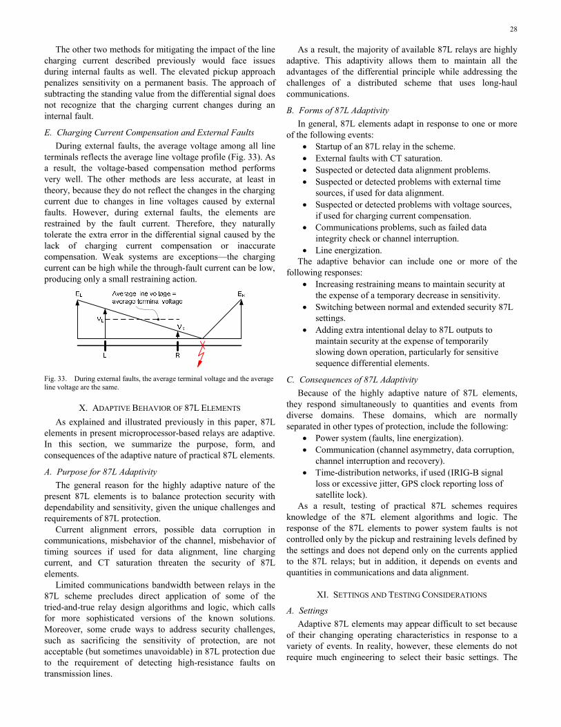
28

The other two methods for mitigating the impact of the line charging current described previously would face issues during internal faults as well. The elevated pickup approach penalizes sensitivity on a permanent basis. The approach of subtracting the standing value from the differential signal does not recognize that the charging current changes during an internal fault.

E. Charging Current Compensation and External Faults During external faults, the average voltage among all line

terminals reflects the average line voltage profile (Fig. 33). As a result, the voltage-based compensation method performs very well. The other methods are less accurate, at least in theory, because they do not reflect the changes in the charging current due to changes in line voltages caused by external faults. However, during external faults, the elements are restrained by the fault current. Therefore, they naturally tolerate the extra error in the differential signal caused by the lack of charging current compensation or inaccurate compensation. Weak systems are exceptions—the charging current can be high while the through-fault current can be low, producing only a small restraining action.

Fig. 33. During external faults, the average terminal voltage and the average line voltage are the same.

X. ADAPTIVE BEHAVIOR OF 87L ELEMENTS As explained and illustrated previously in this paper, 87L

elements in present microprocessor-based relays are adaptive. In this section, we summarize the purpose, form, and consequences of the adaptive nature of practical 87L elements.

A. Purpose for 87L Adaptivity The general reason for the highly adaptive nature of the

present 87L elements is to balance protection security with dependability and sensitivity, given the unique challenges and requirements of 87L protection.

Current alignment errors, possible data corruption in communications, misbehavior of the channel, misbehavior of timing sources if used for data alignment, line charging current, and CT saturation threaten the security of 87L elements.

Limited communications bandwidth between relays in the 87L scheme precludes direct application of some of the tried-and-true relay design algorithms and logic, which calls for more sophisticated versions of the known solutions. Moreover, some crude ways to address security challenges, such as sacrificing the sensitivity of protection, are not acceptable (but sometimes unavoidable) in 87L protection due to the requirement of detecting high-resistance faults on transmission lines.

As a result, the majority of available 87L relays are highly adaptive. This adaptivity allows them to maintain all the advantages of the differential principle while addressing the challenges of a distributed scheme that uses long-haul communications.

B. Forms of 87L Adaptivity In general, 87L elements adapt in response to one or more

of the following events: • Startup of an 87L relay in the scheme. • External faults with CT saturation. • Suspected or detected data alignment problems. • Suspected or detected problems with external time

sources, if used for data alignment. • Suspected or detected problems with voltage sources,

if used for charging current compensation. • Communications problems, such as failed data

integrity check or channel interruption. • Line energization.

The adaptive behavior can include one or more of the following responses:

• Increasing restraining means to maintain security at the expense of a temporary decrease in sensitivity.

• Switching between normal and extended security 87L settings.

• Adding extra intentional delay to 87L outputs to maintain security at the expense of temporarily slowing down operation, particularly for sensitive sequence differential elements.

C. Consequences of 87L Adaptivity Because of the highly adaptive nature of 87L elements,

they respond simultaneously to quantities and events from diverse domains. These domains, which are normally separated in other types of protection, include the following:

• Power system (faults, line energization). • Communication (channel asymmetry, data corruption,

channel interruption and recovery). • Time-distribution networks, if used (IRIG-B signal

loss or excessive jitter, GPS clock reporting loss of satellite lock).

As a result, testing of practical 87L schemes requires knowledge of the 87L element algorithms and logic. The response of the 87L elements to power system faults is not controlled only by the pickup and restraining levels defined by the settings and does not depend only on the currents applied to the 87L relays; but in addition, it depends on events and quantities in communications and data alignment.

XI. SETTINGS AND TESTING CONSIDERATIONS

A. Settings Adaptive 87L elements may appear difficult to set because

of their changing operating characteristics in response to a variety of events. In reality, however, these elements do not require much engineering to select their basic settings. The

29

following three factors contribute to the simplicity of settings selection:

• Typically, only three settings are required: the pickup threshold and the restraining settings, such as the slope (or slopes and the break point) for percentage differential elements or the blocking angle and radius for Alpha Plane elements.

• The differential principle itself makes the settings selection easier by alleviating issues like infeed effect for distance functions, impact of weak terminals, impact of series compensation, current reversal when clearing external faults on parallel lines, or power swings.

• The internal sophistication of present 87L elements allows them to perform very well based on built-in adaptivity. The user-selected basic settings only provide the general boundaries for the balance between sensitivity and security.

In summary, adaptive 87L elements rely on built-in algorithms and logic as much as on user settings. As a result, the differences in the nature of their settings (slopes versus blocking angle or radius) should not be overstated.

B. Testing The adaptive nature of 87L relays increases the complexity

of 87L scheme testing. Reference [18] reviews the many aspects of testing 87L schemes with a focus on field testing (commissioning testing, maintenance testing, and troubleshooting). The following three aspects are worth emphasizing:

• Testing the operating characteristic (with the basic settings of pickup and restraining) confirms the integrity of the scheme and verifies that the intended settings are applied in the relays. This testing is valuable in commissioning. Simple steady-state input signals generated by standard test set software are typically sufficient for these tests. This type of testing, however, does not provide much information related to the actual performance of the 87L element during power system faults.

• When testing for performance as a part of product certification or development, we should apply as realistic inputs to the relays as possible, instead of applying input signals generated by simple means. This procedure verifies that the relay algorithms respond correctly for real power system patterns. Testing with waveforms generated by electromagnetic transient programs, either in closed-loop mode (Real Time Digital Simulator) or in playback mode (output files from EMTP), is recommended when probing the relays for performance.

• When testing for performance, we should simulate events in all three domains to which the elements respond: power system, communications, and timing. This is most conveniently done in closed-loop simulation environments using scripts to coordinate events in all the domains involved (e.g., an external fault followed by a communications path switching 10 milliseconds after the fault inception and before the fault clearance).

XII. CONCLUSION This paper provides a wealth of information on the

algorithms and logic of 87L protection elements available in present microprocessor-based 87L relays.

Unique challenges for 87L schemes, as compared with other types of differential protection, are reviewed in great detail because they are the key driving forces for the internal sophistication and adaptivity of 87L elements.

This paper focuses on percentage differential and Alpha Plane operating characteristics because these two characteristics dominate the actual implementations presently available. Their similarities and differences are reviewed, as well as the relative strengths of each.

The Alpha Plane operating characteristic is able to tolerate greater phase angle errors that may result from current misalignment in 87L applications. On the other hand, the percentage differential operating characteristic allows the manipulation of the differential and restraining signals for the benefit of charging current compensation, cross-phase restraining of sequence differential elements, harmonic restraint in applications with in-line transformers, and so on.

This paper describes a generalized Alpha Plane element. This new technique applies the concept of the restraining signal before transitioning to an equivalent current ratio, thus benefiting from the relative strengths of both the percentage differential principle and the Alpha Plane principle.

Solutions to key challenges in 87L protection, applicable to either percentage differential or Alpha Plane elements, are reviewed in great detail. These challenges include security under external faults with CT saturation, security under current alignment errors, and line charging current. To address these unique challenges of 87L protection, the 87L elements are sophisticated and highly adaptive. The impact of adaptivity on settings selection and testing is also reviewed in this paper.

The 87L elements found in present microprocessor-based relays are optimized for performance rather than built to follow a simple operating characteristic. They perform very well without relying on fine-tuned settings to suit any particular application.

As a matter of fact, the performance of 87L elements depends as much on the algorithms and logic as on user settings. Therefore, knowledge of the algorithms and logic allows for a better grasp of the operating limits of any given 87L element in terms of security and sensitivity, as well as creating better certification programs for new relays.

30

XIII. APPENDIX The single-slope percentage differential characteristic with

a slope of K (0 < K < 1) passing through the origin and corresponding to (4) and (8) can be unambiguously mapped into the Alpha Plane. Equation (87) provides the limiting contour of the restraining region in polar coordinates k k= ∠θ .

( )2 22

2kk cos K 1 01 K

+ θ − + =−

(87)

XIV. REFERENCES [1] H. J. Altuve Ferrer and E. O. Schweitzer, III (eds.), Modern Solutions

for Protection, Control, and Monitoring of Electric Power Systems. Schweitzer Engineering Laboratories, Inc., Pullman, WA, 2010.

[2] H. J. Altuve, J. B. Mooney, and G. E. Alexander, “Advances in Series-Compensated Line Protection,” proceedings of the 35th Annual Western Protective Relay Conference, Spokane, WA, October 2008.

[3] J. Roberts, D. Tziouvaras, G. Benmouyal, and H. J. Altuve, “The Effect of Multiprinciple Line Protection on Dependability and Security,” proceedings of the 55th Annual Georgia Tech Protective Relaying Conference, Atlanta, GA, May 2001.

[4] B. Kasztenny, N. Fischer, K. Fodero, and A. Zvarych, “Communications and Data Synchronization for Line Current Differential Schemes,” proceedings of the 38th Annual Western Protective Relay Conference, Spokane, WA, October 2011.

[5] H. P. Sleeper, “Ratio Differential Relay Protection,” Electrical World, October 1927, pp. 827–831.

[6] M. J. Thompson, “Percentage Restrained Differential, Percentage of What?” proceedings of the 64th Annual Conference for Protective Relay Engineers, College Station, TX, April 2011.

[7] G. Ziegler, Numerical Differential Protection: Principles and Applications. Publicis Corporate Publishing, Erlangen, Germany, 2005.

[8] H. Miller, J. Burger, N. Fischer, and B. Kasztenny, “Modern Line Current Differential Protection Solutions,” proceedings of the 63rd Annual Conference for Protective Relay Engineers, College Station, TX, March 2010.

[9] A. R. van C. Warrington, Protective Relays: Their Theory and Practice, Vol. 1. Chapman and Hall Ltd., London, England, 1962.

[10] D. A. Tziouvaras, H. Altuve, G. Benmouyal, and J. Roberts, “Line Differential Protection With an Enhanced Characteristic,” proceedings of Med Power 2002, Athens, Greece, November 2002.

[11] G. Benmouyal and T. Lee, “Securing Sequence-Current Differential Elements,” proceedings of the 31st Annual Western Protective Relay Conference, Spokane, WA, October 2004.

[12] A. Guzmán, C. Labuschagne, and B. L. Qin, “Reliable Busbar and Breaker Failure Protection With Advanced Zone Selection,” proceedings of the 31st Annual Western Protective Relay Conference, Spokane, WA, October 2004.

[13] G. Benmouyal and J. Roberts, “Superimposed Quantities: Their True Nature and Application in Relays,” proceedings of the 26th Annual Western Protective Relay Conference, Spokane, WA, October 1999.

[14] K. Fodero, C. Huntley, and D. Whitehead, “Secure, Wide-Area Time Synchronization,” proceedings of the 12th Annual Western Power Delivery Automation Conference, Spokane, WA, April 2010.

[15] M. G. Adamiak, G. E. Alexander, and W. Premerlani, “A New Approach to Current Differential Protection for Transmission Lines,” proceedings of the 53rd Annual Georgia Tech Protective Relaying Conference, Atlanta, GA, May 1999.

[16] Z. Gajic, I. Brncic, and F. Rios, “Multi-Terminal Line Differential Protection With Innovative Charging Current Compensation Algorithm,” proceedings of the 10th Developments in Power System Protection Conference, March 2010.

[17] E. O. Schweitzer, III, N. Fischer, and B. Kasztenny, “A Fresh Look at Limits to the Sensitivity of Line Protection,” proceedings of the 37th Annual Western Protective Relay Conference, Spokane, WA, October 2010.

[18] D. Finney, N. Fischer, B. Kasztenny, and K. Lee, “Testing Considerations for Line Current Differential Schemes,” proceedings of the 38th Annual Western Protective Relay Conference, Spokane, WA, October 2011.

XV. BIOGRAPHIES Bogdan Kasztenny is a principal systems engineer in the research and development division of Schweitzer Engineering Laboratories, Inc. He has over 20 years of expertise in power system protection and control, including ten years of academic career and ten years of industrial experience, developing, promoting, and supporting many protection and control products. Bogdan is an IEEE Fellow, Senior Fulbright Fellow, Canadian member of CIGRE Study Committee B5, registered professional engineer in the province of Ontario, and an adjunct professor at the University of Western Ontario. Since 2011, Bogdan has served on the Western Protective Relay Conference Program Committee. Bogdan has authored about 200 technical papers and holds 20 patents.

Gabriel Benmouyal, P.E., received his BASc in electrical engineering and his MASc in control engineering from Ecole Polytechnique, Université de Montréal, Canada, in 1968 and 1970. In 1969, he joined Hydro-Québec as an instrumentation and control specialist. He worked on different projects in the fields of substation control systems and dispatching centers. In 1978, he joined IREQ, where his main fields of activity were the application of microprocessors and digital techniques for substations and generating station control and protection systems. In 1997, he joined Schweitzer Engineering Laboratories, Inc. as a principal research engineer. Gabriel is a registered professional engineer in the province of Québec and an IEEE senior member and has served on the Power System Relaying Committee since May 1989. He holds over six patents and is the author or coauthor of several papers in the fields of signal processing and power network protection and control.

Héctor J. Altuve received his BSEE degree in 1969 from the Central University of Las Villas in Santa Clara, Cuba, and his Ph.D. in 1981 from Kiev Polytechnic Institute in Kiev, Ukraine. From 1969 until 1993, Dr. Altuve served on the faculty of the Electrical Engineering School at the Central University of Las Villas. From 1993 to 2000, he served as professor of the Graduate Doctoral Program in the Mechanical and Electrical Engineering School at the Autonomous University of Nuevo León in Monterrey, Mexico. In 1999 through 2000, he was the Schweitzer Visiting Professor in the Department of Electrical Engineering at Washington State University. Dr. Altuve joined Schweitzer Engineering Laboratories, Inc. in January 2001, where he is currently a distinguished engineer and director of technology for Latin America. He has authored and coauthored more than 100 technical papers and several books and holds four patents. His main research interests are in power system protection, control, and monitoring. Dr. Altuve is an IEEE senior member.

Normann Fischer received a Higher Diploma in Technology, with honors, from Witwatersrand Technikon, Johannesburg in 1988, a BSEE, with honors, from the University of Cape Town in 1993, and an MSEE from the University of Idaho in 2005. He joined Eskom as a protection technician in 1984 and was a senior design engineer in the Eskom protection design department for three years. He then joined IST Energy as a senior design engineer in 1996. In 1999, he joined Schweitzer Engineering Laboratories, Inc. as a power engineer in the research and development division. Normann was a registered professional engineer in South Africa and a member of the South Africa Institute of Electrical Engineers. He is currently a member of IEEE and ASEE.

© 2011 by Schweitzer Engineering Laboratories, Inc. All rights reserved.

20111101 • TP6511-01