Embed Size (px)
Citation preview
Truncated Normal Collocation:(Chasing the One-Armed Man)
John BurkardtDepartment of Scientific Computing
Florida State University..........
3:30-4:45pm, 14 February 2014,Graduate Student Seminar ISC5934
..........http://people.sc.fsu.edu/∼jburkardt/presentations/
truncated normal 2014 fsu.pdf
1 / 55

INTRO:
In a prehistoric TV series called ”The Fugitive”, Dr Richard Kimble,falsely accused of murdering his wife, searched for the one-armed manwho was the real killer.
There are no murders scheduled for today, but I will be lopping off theright arm, the left arm, or both arms, of the standard normal distribution!
2 / 55
Truncated Normal Collocation
The Strange Case of the Abnormal Normal
Can You Describe the Suspect?
I Have a Cunning Plan
A Matter of Moments
The Summing Up
3 / 55
ABNORMAL: The Normal Probability Distribution
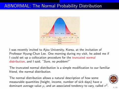
I was recently invited to Ajou University, Korea, at the invitation ofProfessor Hyung-Chun Lee. One morning during my visit, he asked me ifI could set up a collocation procedure for the truncated normaldistribution, and I said, ”Sure, no problem!”
The truncated normal distribution is a simple modification to our familiarfriend, the normal distribution.
The normal distribution allows a natural description of how somemeasurable quantities (height, income, number of sick days) have adominant average value µ, and an associated tendency to vary, called σ2.
4 / 55
ABNORMAL: The Truncated Normal
Mathematical models are idealizations, and have their limitations. Ifwe think the normal distribution is a good model of height distribution,then strictly speaking, we are admitting the possibility (small, but notzero!) of people who are as tall as 60 or 1000 feet - or negative 200 feet,for that matter.
This discrepancy could be a problem if we are doing a simulation, forinstance. Then we treat the mathematical distribution as physcial reality,we sample it, and we “believe” whatever comes out of the process. If wecreate a 1-inch person, then we are now stuck dealing with a physicallymeaningless but computationally real object.
5 / 55
ABNORMAL: The Truncated Normal
Sometimes these 1 inch people can actually cause the computation tocrash, or to produce meaningless results.
In our research group, a commonly studied problem involves thesimulation of the permeability function a(ω, x) related to groundwaterflow, arising in the equation:
∇ · (a(ω, x)∇u(x)) = f (x)
Mathematically, a solution to this problem can be guaranteed to exist aslong as the permeability function is everywhere positive, bounded awayfrom 0 and from infinity:
0 < amin ≤ a(ω, x) ≤ amax <∞
6 / 55
ABNORMAL: The Log-Normal Probability Distribution
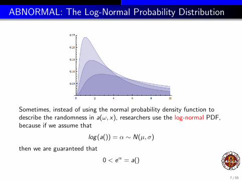
Sometimes, instead of using the normal probability density function todescribe the randomness in a(ω, x), researchers use the log-normal PDF,because if we assume that
log(a()) = α ∼ N(µ, σ)
then we are guaranteed that
0 < eα = a()
7 / 55
ABNORMAL: The Log-Normal Probability Distribution
If we use the log-normal PDF in this way, our simulation will neverselect a negative value for a(), and a() is described by a mathematicallytractable and plausible formula.
But while a() can’t be zero, it can get arbitrarily small or large, meaningthe mathematical requirement was not really guaranteed, and numericallywe may have issues with stability or ill-conditioning.
The distribution is also clearly a different shape from the normaldistribution; it’s not symmetric, and has different variance properties,
Rather than go to a new distribution, researchers have also consideredkeeping the normal distribution, but altering it in some simple way toavoid the problem areas.
8 / 55
ABNORMAL: The Truncated Normal Distribution
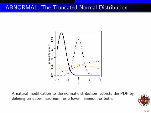
A natural modification to the normal distribution restricts the PDF bydefining an upper maximum, or a lower minimum or both.
9 / 55
ABNORMAL: The Truncated Normal Distribution
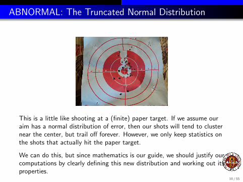
This is a little like shooting at a (finite) paper target. If we assume ouraim has a normal distribution of error, then our shots will tend to clusternear the center, but trail off forever. However, we only keep statistics onthe shots that actually hit the paper target.
We can do this, but since mathematics is our guide, we should justify ourcomputations by clearly defining this new distribution and working out itsproperties.
10 / 55
ABNORMAL: Parameters
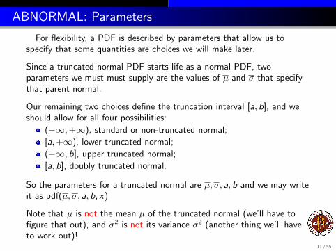
For flexibility, a PDF is described by parameters that allow us tospecify that some quantities are choices we will make later.
Since a truncated normal PDF starts life as a normal PDF, twoparameters we must must supply are the values of µ and σ that specifythat parent normal.
Our remaining two choices define the truncation interval [a, b], and weshould allow for all four possibilities:
(−∞,+∞), standard or non-truncated normal;
[a,+∞), lower truncated normal;
(−∞, b], upper truncated normal;
[a, b], doubly truncated normal.
So the parameters for a truncated normal are µ, σ, a, b and we may writeit as pdf(µ, σ, a, b; x)
Note that µ is not the mean µ of the truncated normal (we’ll have tofigure that out), and σ2 is not its variance σ2 (another thing we’ll haveto work out)!
11 / 55
Truncated Normal Collocation
The Strange Case of the Abnormal Normal
Can You Describe the Suspect?
I Have a Cunning Plan
A Matter of Moments
The Summing Up
12 / 55
DESCRIBE: PDF/CDF/invCDF/SAMPLE/MEAN/VAR
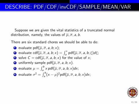
Suppose we are given the vital statistics of a truncated normaldistribution, namely, the values of µ, σ, a, b.
There are six standard chores we should be able to do:
1 evaluate pdf(µ, σ, a, b; x);2 evaluate cdf(µ, σ, a, b; x) =
∫ x
apdf(µ, σ, a, b; ξ)dξ;
3 solve C = cdf(µ, σ, a, b; x) for the value of x ;4 uniformly sample pdf(µ, σ, a, b; x).
5 evaluate µ =∫ b
ax pdf(µ, σ, a, b; x)dx ;
6 evaluate σ2 =∫ b
a(x − µ)2pdf(µ, σ, a, b; x)dx ;
13 / 55
DESCRIBE: PDF
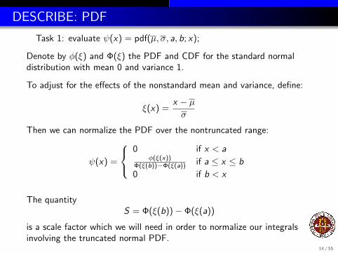
Task 1: evaluate ψ(x) = pdf(µ, σ, a, b; x);
Denote by φ(ξ) and Φ(ξ) the PDF and CDF for the standard normaldistribution with mean 0 and variance 1.
To adjust for the effects of the nonstandard mean and variance, define:
ξ(x) =x − µσ
Then we can normalize the PDF over the nontruncated range:
ψ(x) =
0 if x < a
φ(ξ(x))Φ(ξ(b))−Φ(ξ(a)) if a ≤ x ≤ b
0 if b < x
The quantityS = Φ(ξ(b))− Φ(ξ(a))
is a scale factor which we will need in order to normalize our integralsinvolving the truncated normal PDF.
14 / 55
DESCRIBE: CDF
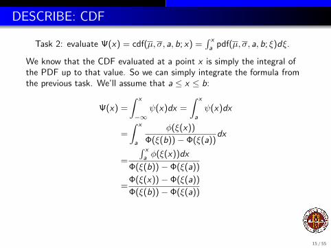
Task 2: evaluate Ψ(x) = cdf(µ, σ, a, b; x) =∫ x
apdf(µ, σ, a, b; ξ)dξ.
We know that the CDF evaluated at a point x is simply the integral ofthe PDF up to that value. So we can simply integrate the formula fromthe previous task. We’ll assume that a ≤ x ≤ b:
Ψ(x) =
∫ x
−∞ψ(x)dx =
∫ x
a
ψ(x)dx
=
∫ x
a
φ(ξ(x))
Φ(ξ(b))− Φ(ξ(a))dx
=
∫ x
aφ(ξ(x))dx
Φ(ξ(b))− Φ(ξ(a))
=Φ(ξ(x))− Φ(ξ(a))
Φ(ξ(b))− Φ(ξ(a))
15 / 55
DESCRIBE: CDF
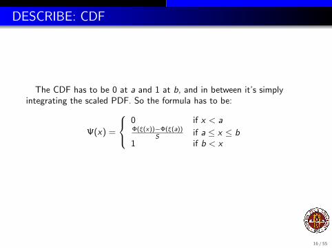
The CDF has to be 0 at a and 1 at b, and in between it’s simplyintegrating the scaled PDF. So the formula has to be:
Ψ(x) =
0 if x < aΦ(ξ(x))−Φ(ξ(a))
S if a ≤ x ≤ b1 if b < x
16 / 55
DESCRIBE: invCDF
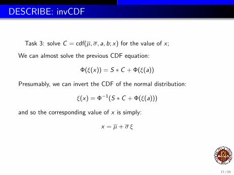
Task 3: solve C = cdf(µ, σ, a, b; x) for the value of x ;
We can almost solve the previous CDF equation:
Φ(ξ(x)) = S ∗ C + Φ(ξ(a))
Presumably, we can invert the CDF of the normal distribution:
ξ(x) = Φ−1(S ∗ C + Φ(ξ(a)))
and so the corresponding value of x is simply:
x = µ+ σ ξ
17 / 55
DESCRIBE: SAMPLE
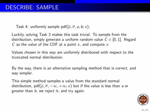
Task 4: uniformly sample pdf(µ, σ, a, b; x);
Luckily, solving Task 3 makes this task trivial. To sample from thedistribution, simply generate a uniform random value C ∈ [0, 1]. RegardC as the value of the CDF at a point x , and compute x .
Values chosen in this way are uniformly distributed with respect to thetruncated normal distribution.
By the way, there is an alternative sampling method that is correct, andway simpler.
This simple method samples a value from the standard normaldistribution, pdf(µ, σ,−∞,+∞; x) but if the value is less than a orgreater than b, we reject it, and try again.
18 / 55
DESCRIBE: SAMPLE (Bad Approach)
The nice thing about the simple “rejection” method is that it is trivialto program. If you can generate random normal numbers, you cangenerate random truncated normal numbers by throwing away the onesyou can’t use.
The drawback is that the amount of work needed to compute a samplegrows enormously as the truncation interval moves around.
We might imagine our typical truncation interval is something like[-5,+5] so we only throw away data that is 5 standard deviations off.
But we should be able to use the same program to sample in the interval[+5,+6], in which case we need to throw away all the data that is lessthan 5 standard deviations from the mean, and more. That program willtake forever to run.
So we really would prefer a sampling method that takes about the sametime to produce 1,000 samples, no matter what truncation interval wespecify. And we can do this.
19 / 55
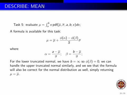
DESCRIBE: MEAN
Task 5: evaluate µ =∫ b
ax pdf(µ, σ, a, b; x)dx ;
A formula is available for this task:
µ = µ+φ(α)− φ(β)
Sσ
where
α =a− µσ
; β =b − µσ
;
For the lower truncated normal, we have b =∞ so φ(β) = 0; we canhandle the upper truncated normal similarly, and we see that the formulawill also be correct for the normal distribution as well, simply returningµ = µ.
20 / 55
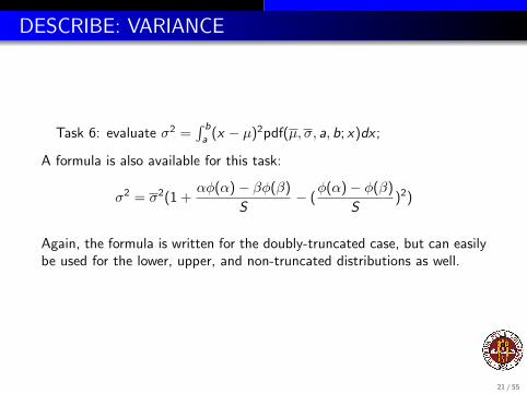
DESCRIBE: VARIANCE
Task 6: evaluate σ2 =∫ b
a(x − µ)2pdf(µ, σ, a, b; x)dx ;
A formula is also available for this task:
σ2 = σ2(1 +αφ(α)− βφ(β)
S− (
φ(α)− φ(β)
S)2)
Again, the formula is written for the doubly-truncated case, but can easilybe used for the lower, upper, and non-truncated distributions as well.
21 / 55
DESCRIBE: Checking the Facts
I set up a library called truncated normal which included code for thesix tasks, for all four truncation possibilities,
Now I figured I needed some confidence in my formulas before movingon, so I constructed a set of tests.
One simple test is to start with a value of X, compute its CDF, thencompute invCDF and see if we get back to X.
The second test was to do a simulation. That is, use the SAMPLEfunction to compute, say, 10,000 sample values of a distribution,compute the sample mean and variance, and compare them to theMEAN and VARIANCE functions.
After banging on the code, the tests behaved, and I felt much better.
http://people.sc.fsu.edu/∼jburkardt/m src/truncated normal/truncated normal.html
22 / 55
DESCRIBE: You’re Not Done!
I kept busy all morning long working out these details about thetruncated normal distribution and trying to program, document, and testthem.
That afternoon, Professor Lee came back into the office and asked if Ihad been able to complete the collocation task.
”Well...”, I said hesitantly, ”I can PDF, CDF, invCDF, SAMPLE, MEANand VARIANCE.”
”What about the collocation?” he asked.
”Actually,” I said, ”I might need one more day...”
As it turned out, I ended up working on this problem for another month.
23 / 55

Truncated Normal Collocation
The Strange Case of the Abnormal Normal
Can You Describe the Suspect?
I Have a Cunning Plan
A Matter of Moments
The Summing Up
24 / 55
PLAN: What Do We Need?
We weren’t pursuing the truncated normal distribution for its own sake- what we were really after was the ability to do collocation.
We wanted to estimate the expected value of “quantities of interest”associated with a system of partial differential equations that includedstochastic input terms.
The stochastic input terms were going to be modeled by truncatednormal distributions, so that they behaved like normal variables, but overa truncated range.
In order to estimate the quantities of interest, a collocation procedureselects many test values of the input terms, weighted by theirprobabilities, and computes an average that is really a multidimensionalintegral.
25 / 55
PLAN: We Need a Quadrature Rule
If every input term is controlled by a truncated normal distribution,then the crucial tool we need is a sequence of quadrature rules, ofincreasing accuracy, for that distribution.
A quadrature rule for the truncated normal distribution is a set of npoints xi and weights wi for which we make the estimate
1
S√
2πσ2
∫ b
a
f (x)e−(x−µ)2
2σ2 dx ≈n∑
i=1
wi · f (xi )
We are usually looking for a quadrature rule of Gaussian type, so that then-point rule will integrate precisely any function f (x) which is apolynomial of degree 2n − 1 or less.
Analytic formulas are known for special weight functions; otherwise, afamous paper by Golub and Welsch shows how to construct a matrixwhose eigendecomposition will produce the desired rule.
26 / 55
PLAN: Orthogonal Polynomial Family
The most common algorithm described by Golub and Welsch assumesthat the user knows a family of polynomials φi (x), i = 0, ... which areorthogonal with respect to the PDF.
To explain what is going on, let us suppose that we use our PDF todefine a new inner product of any two functions f () and g() by:
< f , g >≡∫ +∞
−∞f (x)g(x) pdf(µ, σ, a, b; x)dx
We can define a corresponding function norm:
||f || =√< f , f >
in which case we will want to restrict our attention to the space of allfunctions whose norm is finite.
27 / 55
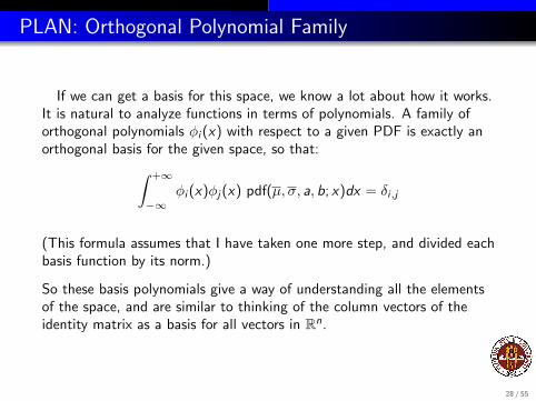
PLAN: Orthogonal Polynomial Family
If we can get a basis for this space, we know a lot about how it works.It is natural to analyze functions in terms of polynomials. A family oforthogonal polynomials φi (x) with respect to a given PDF is exactly anorthogonal basis for the given space, so that:∫ +∞
−∞φi (x)φj(x) pdf(µ, σ, a, b; x)dx = δi,j
(This formula assumes that I have taken one more step, and divided eachbasis function by its norm.)
So these basis polynomials give a way of understanding all the elementsof the space, and are similar to thinking of the column vectors of theidentity matrix as a basis for all vectors in Rn.
28 / 55
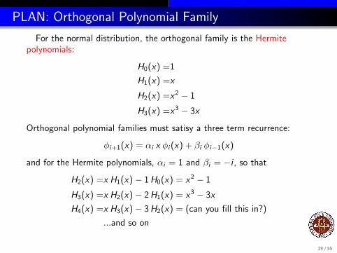
PLAN: Orthogonal Polynomial Family
For the normal distribution, the orthogonal family is the Hermitepolynomials:
H0(x) =1
H1(x) =x
H2(x) =x2 − 1
H3(x) =x3 − 3x
Orthogonal polynomial families must satisy a three term recurrence:
φi+1(x) = αi x φi (x) + βi φi−1(x)
and for the Hermite polynomials, αi = 1 and βi = −i , so that
H2(x) =x H1(x)− 1 H0(x) = x2 − 1
H3(x) =x H2(x)− 2 H1(x) = x3 − 3x
H4(x) =x H3(x)− 3 H2(x) = (can you fill this in?)
...and so on
29 / 55
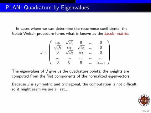
PLAN: Quadrature by Eigenvalues
In cases where we can determine the recurrence coefficients, theGolub-Welsch procedure forms what is known as the Jacobi matrix:
J =
α0
√β1 0 ... 0√
β1 α1
√β2 ... 0
0√β2 α2 ... 0
... ... ... ... ...0 0 0 ... αn−1
The eigenvalues of J give us the quadrature points; the weights arecomputed from the first components of the normalized eigenvectors.
Because J is symmetric and tridiagonal, the computation is not difficult,so it might seem we are all set...
30 / 55
PLAN: Truncated Normal is a Problem
Unfortunately, the Hermite polynomials Hi (x) are the correctorthogonal family for the normal distribution, but not for the truncatednormal distribution;
I don’t know the family for the truncated distribution.
And remember, we say “the” truncated normal distribution, but everychoice of the parameters µ, σ, a, b really gives us a completely differentdistribution, and presumably a different orthogonal family to work out...ifwe could work it out.
Fortunately, the orthogonal family method is not the only way.
Golub and Welsch described an alternative, the moment matrix method.
31 / 55
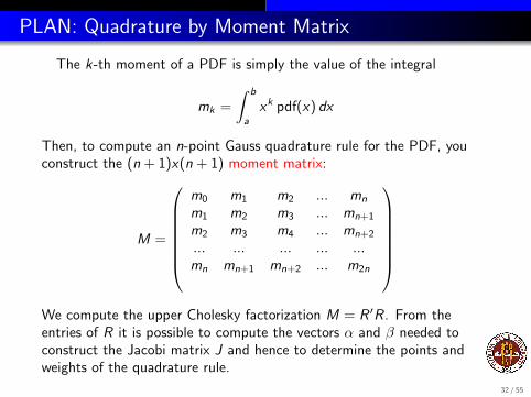
PLAN: Quadrature by Moment Matrix
The k-th moment of a PDF is simply the value of the integral
mk =
∫ b
a
xk pdf(x) dx
Then, to compute an n-point Gauss quadrature rule for the PDF, youconstruct the (n + 1)x(n + 1) moment matrix:
M =
m0 m1 m2 ... mn
m1 m2 m3 ... mn+1
m2 m3 m4 ... mn+2
... ... ... ... ...mn mn+1 mn+2 ... m2n
We compute the upper Cholesky factorization M = R ′R. From theentries of R it is possible to compute the vectors α and β needed toconstruct the Jacobi matrix J and hence to determine the points andweights of the quadrature rule.
32 / 55
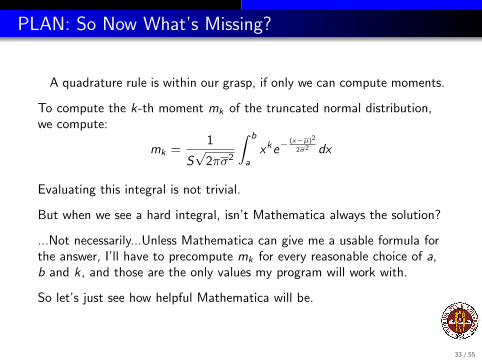
PLAN: So Now What’s Missing?
A quadrature rule is within our grasp, if only we can compute moments.
To compute the k-th moment mk of the truncated normal distribution,we compute:
mk =1
S√
2πσ2
∫ b
a
xke−(x−µ)2
2σ2 dx
Evaluating this integral is not trivial.
But when we see a hard integral, isn’t Mathematica always the solution?
...Not necessarily...Unless Mathematica can give me a usable formula forthe answer, I’ll have to precompute mk for every reasonable choice of a,b and k , and those are the only values my program will work with.
So let’s just see how helpful Mathematica will be.
33 / 55
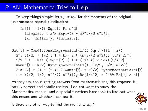
PLAN: Mathematica Tries to Help
To keep things simple, let’s just ask for the moments of the originalun-truncated normal distribution:
In[1] = 1/(S Sqrt[2 Pi s^2]Integrate [ x^k Exp[-(x - m)^2/(2 s^2)],{x, -Infinity, +Infinity}]
Out[1] = ConditionalExpression[(1/(S Sqrt[\[Pi]] s))2^(-(1/2) + 1/2 (-1 + k)) E^(-(m^2/(2 s^2))) (1/s^2)^(1/2 (-1 - k)) (-Sqrt[2] (-1 + (-1)^k) m Sqrt[1/s^2]Gamma[1 + k/2] Hypergeometric1F1[1 + k/2, 3/2, m^2/(2 s^2)] + (1 + (-1)^k) Gamma[(1 + k)/2] Hypergeometric1F1[(1 + k)/2, 1/2, m^2/(2 s^2)]), Re[1/s^2] > 0 && Re[k] > -1]
As they say about getting answers from mathematicians, this response istotally correct and totally useless! I do not want to study theMathematica manual and a special functions handbook to find out whatthis means and whether I can use it.
Is there any other way to find the moments mk?34 / 55
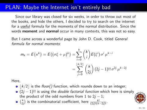
PLAN: Maybe the Internet isn’t entirely bad
Since our library was closed for six weeks, in order to throw out most ofthe books, and hide the others, I decided to try to search on the internetfor a useful formula for the moments of the normal distribution. Since thewords moment and normal occur in many contexts, this was not so easy.
But I came across a wonderful page by John D. Cook, titled Generalformula for normal moments:
mk = E{xk} = E{(σξ + µ)k} =k∑
i=0
(k
i
)E (ξi )σi µk−i
=
bk/2c∑j=0
(k
2j
)(2j − 1)!!σ2j µk−2j
Here,
bk/2c is the floor() function, which rounds down to an integer;
(2j − 1)!! is using the double factorial function which here is simplythe product of the odd numbers from 1 to 2j − 1;(
k2j
)is the combinatorial coefficient, here k!
(2j)!(k−2j)! .
35 / 55
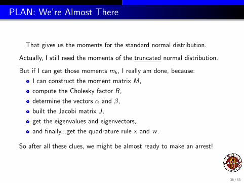
PLAN: We’re Almost There
That gives us the moments for the standard normal distribution.
Actually, I still need the moments of the truncated normal distribution.
But if I can get those moments mk , I really am done, because:
I can construct the moment matrix M,
compute the Cholesky factor R,
determine the vectors α and β,
built the Jacobi matrix J,
get the eigenvalues and eigenvectors,
and finally...get the quadrature rule x and w .
So after all these clues, we might be almost ready to make an arrest!
36 / 55

Truncated Normal Collocation
The Strange Case of the Abnormal Normal
Can You Describe the Suspect?
I Have a Cunning Plan
A Matter of Moments
The Summing Up
37 / 55
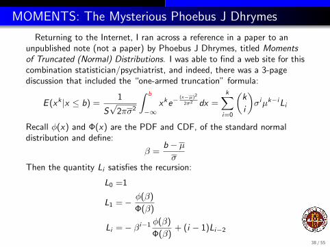
MOMENTS: The Mysterious Phoebus J Dhrymes
Returning to the Internet, I ran across a reference in a paper to anunpublished note (not a paper) by Phoebus J Dhrymes, titled Momentsof Truncated (Normal) Distributions. I was able to find a web site for thiscombination statistician/psychiatrist, and indeed, there was a 3-pagediscussion that included the “one-armed truncation” formula:
E (xk |x ≤ b) =1
S√
2πσ2
∫ b
−∞xke−
(x−µ)2
2σ2 dx =k∑
i=0
(k
i
)σiµk−iLi
Recall φ(x) and Φ(x) are the PDF and CDF, of the standard normaldistribution and define:
β =b − µσ
Then the quantity Li satisfies the recursion:
L0 =1
L1 =− φ(β)
Φ(β)
Li =− βi−1 φ(β)
Φ(β)+ (i − 1)Li−2
38 / 55
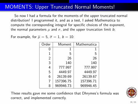
MOMENTS: Upper Truncated Normal Moments!
So now I had a formula for the moments of the upper truncated normaldistribution! I programmed it, and as a test, I asked Mathematica tocompute the corresponding integral for specific choices of the exponent,the normal parameters µ and σ, and the upper truncation limit b;
For example, for µ = 5, σ = 1, b = 10:
Order Moment Mathematica0 1 11 5 52 26 263 140 1404 777.997 777.9975 4449.97 4449.976 26139.69 26139.677 157396.75 157396.718 969946.73 969946.45
These results gave me some confidence that Dhrymes’s formula wascorrect, and implemented correctly.
39 / 55
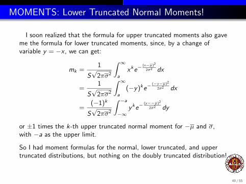
MOMENTS: Lower Truncated Normal Moments!
I soon realized that the formula for upper truncated moments also gaveme the formula for lower truncated moments, since, by a change ofvariable y = −x , we can get:
mk =1
S√
2πσ2
∫ ∞a
xke−(x−µ)2
2σ2 dx
=1
S√
2πσ2
∫ ∞a
(−y)ke−(−y−µ)2
2σ2 dx
=(−1)k
S√
2πσ2
∫ −a
−∞yke−
(y−−µ)2
2σ2 dy
or ±1 times the k-th upper truncated normal moment for −µ and σ,with −a as the upper limit.
So I had moment formulas for the normal, lower truncated, and uppertruncated distributions, but nothing on the doubly truncated distribution!
40 / 55
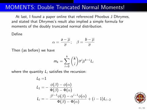
MOMENTS: Double Truncated Normal Moments!
At last, I found a paper online that referenced Phoebus J Dhrymes,and stated that Dhrymes’s result also implied a simple formula formoments of the doubly truncated normal distribution.
Define
α =a− µσ
; β =b − µσ
Then (as before) we have
mk =k∑
i=0
(k
i
)σiµk−iLi
where the quantity Li satisfies the recursion:
L0 =1
L1 =− φ(β)− φ(α)
Φ(β)− Φ(α)
Li =− βi−1φ(β)− αi−1φ(α)
Φ(β)− Φ(α)+ (i − 1)Li−2
41 / 55
MOMENTS: Double Truncated Normal Moments!
Now that I had usable moment formulas for all four cases, I added aseventh “task”, to compute the k-th moment, to the truncated normallibrary.
And I was now ready to consider the next step, which was to implementthe moment formulation of the Golub-Welsch algorithm for computingquadrature rules.
http://people.sc.fsu.edu/∼jburkardt/m src/truncated normal/truncated normal.html
42 / 55
Truncated Normal Collocation
The Strange Case of the Abnormal Normal
Can You Describe the Suspect?
I Have a Cunning Plan
A Matter of Moments
The Summing Up
43 / 55
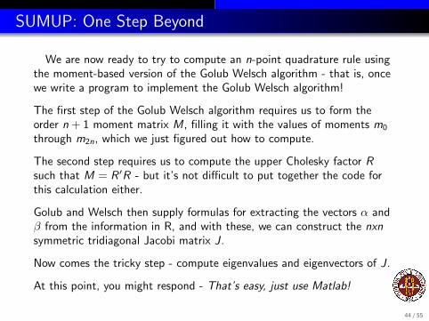
SUMUP: One Step Beyond
We are now ready to try to compute an n-point quadrature rule usingthe moment-based version of the Golub Welsch algorithm - that is, oncewe write a program to implement the Golub Welsch algorithm!
The first step of the Golub Welsch algorithm requires us to form theorder n + 1 moment matrix M, filling it with the values of moments m0
through m2n, which we just figured out how to compute.
The second step requires us to compute the upper Cholesky factor Rsuch that M = R ′R - but it’s not difficult to put together the code forthis calculation either.
Golub and Welsch then supply formulas for extracting the vectors α andβ from the information in R, and with these, we can construct the nxnsymmetric tridiagonal Jacobi matrix J.
Now comes the tricky step - compute eigenvalues and eigenvectors of J.
At this point, you might respond - That’s easy, just use Matlab!
44 / 55
SUMUP: Jacobi will get me the eigenvalues
I want my code to be accessible in several languages. So I really wantto write down an eigenvalue routine explicitly. Luckily, our symmetricmatrix J is ideal for the Jacobi eigenvalue algorithm.
The basic idea of the Jacobi algorithm is to pre- and post-multiply thematrix by Jacobi rotation matrices that zero out the largest off-diagonalelement. As this process is repeated, the matrix rapidly approximates adiagonal matrix, from which the eigenvalues can be read off.
Moreover, I had forgotten that this algorithm can also return thecorresponding eigenvectors, which we need to have for the quadratureweights.
So my next task was to write a library called jacobi eigenvalue whichwould allow me to test my implementation on some standard problems.
http://people.sc.fsu.edu/∼jburkardt/m src/jacobi eigenvalue/jacobi eigenvalue.html
45 / 55
SUMUP: The Golub-Welsch Moment Algorithm Executes
Once the Jacobi eigenvalue algorithm was working, I had all the piecesneeded to carry out a Golub-Welsch momentum algorithm.
Since I had never done this before, I first set up momentum calculationsfor Legendre, Laguerre, and Normal distributions, because I knew whatthe associated quadrature rules should be in these cases, and I caughtsome small errors this way.
Then I added in the momentum calculations for the truncated normaldistribution, and was finally able to compute some example rules.
I called this hunk of software quadmom for quadrature by moments.
http://people.sc.fsu.edu/∼jburkardt/m src/quadmom/quadmom.html
46 / 55
SUMUP: An Interactive Rule Calculator
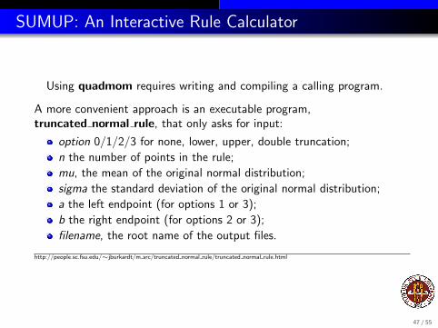
Using quadmom requires writing and compiling a calling program.
A more convenient approach is an executable program,truncated normal rule, that only asks for input:
option 0/1/2/3 for none, lower, upper, double truncation;
n the number of points in the rule;
mu, the mean of the original normal distribution;
sigma the standard deviation of the original normal distribution;
a the left endpoint (for options 1 or 3);
b the right endpoint (for options 2 or 3);
filename, the root name of the output files.
http://people.sc.fsu.edu/∼jburkardt/m src/truncated normal rule/truncated normal rule.html
47 / 55
SUMUP: An Interactive Rule Calculator
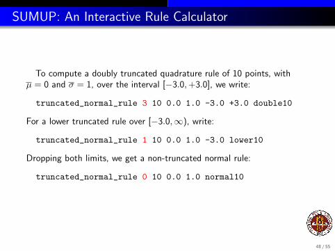
To compute a doubly truncated quadrature rule of 10 points, withµ = 0 and σ = 1, over the interval [−3.0,+3.0], we write:
truncated_normal_rule 3 10 0.0 1.0 -3.0 +3.0 double10
For a lower truncated rule over [−3.0,∞), write:
truncated_normal_rule 1 10 0.0 1.0 -3.0 lower10
Dropping both limits, we get a non-truncated normal rule:
truncated_normal_rule 0 10 0.0 1.0 normal10
48 / 55
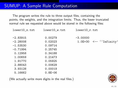
SUMUP: A Sample Rule Computation
The program writes the rule to three output files, containing thepoints, the weights, and the integration limits. Thus, the lower truncatednormal rule we requested above would be stored in the following files:
lower10_x.txt lower10_w.txt lower10_r.txt
-2.83915 0.00279 -3.00000-2.28008 0.02023 1.0E+30 <-- ‘‘Infinity’’-1.53530 0.09714-0.71994 0.257450.12958 0.341881.00659 0.214731.91770 0.059252.88043 0.006293.93128 0.000195.16662 0.8E-06
(We actually write more digits in the real files.)
49 / 55
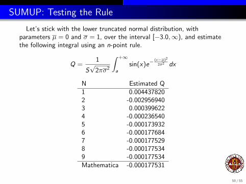
SUMUP: Testing the Rule
Let’s stick with the lower truncated normal distribution, withparameters µ = 0 and σ = 1, over the interval [−3.0,∞), and estimatethe following integral using an n-point rule.
Q =1
S√
2πσ2
∫ +∞
a
sin(x)e−(x−µ)2
2σ2 dx
N Estimated Q1 0.0044378202 -0.0029569403 0.0003996224 -0.0002365405 -0.0001739326 -0.0001776847 -0.0001775298 -0.0001775349 -0.000177534Mathematica -0.000177531
50 / 55
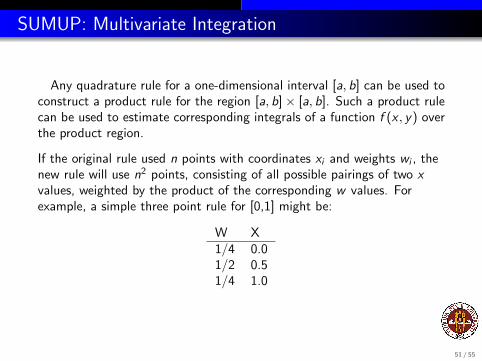
SUMUP: Multivariate Integration
Any quadrature rule for a one-dimensional interval [a, b] can be used toconstruct a product rule for the region [a, b]× [a, b]. Such a product rulecan be used to estimate corresponding integrals of a function f (x , y) overthe product region.
If the original rule used n points with coordinates xi and weights wi , thenew rule will use n2 points, consisting of all possible pairings of two xvalues, weighted by the product of the corresponding w values. Forexample, a simple three point rule for [0,1] might be:
W X1/4 0.01/2 0.51/4 1.0
51 / 55
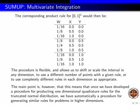
SUMUP: Multivariate Integration
The corresponding product rule for [0, 1]2 would then be:
W X Y1/16 0.0 0.01/8 0.5 0.01/16 1.0 0.01/8 0.0 0.51/4 0.5 0.51/8 1.0 0.51/16 0.0 1.01/8 0.5 1.01/16 1.0 1.0
The procedure is flexible, and allows us to shift or scale the interval inany dimension, to use a different number of points with a given rule, orto use completely different rules in each dimension as appropriate.
The main point is, however, that this means that once we have developeda procedure for producting one dimensional quadrature rules for thetruncated normal distribution, we have automatically a procedure forgenerating similar rules for problems in higher dimensions.
52 / 55
SUMUP: Sparse Grids
If we are interested in multivariate integration, then technically theproduct rule approach gives us everything we need. However, notice thatthe number of points used by a product rule involves raising the numberof points in the 1D rule to the power of the dimension. While a 3 pointrule in 1D looks cheap, in 10 dimenension it needs almost 60,000 pointsand more than 3 billion points in 20 dimensions.
When modeling stochastic problems, each random variable correspondsto a dimension, and it’s not uncommon for users to want 40 or 50 suchvariables. This would seem to rule out the use of standard quadraturerules, leaving nothing but Monte Carlo sampling to estimate theintegrals.
53 / 55
SUMUP: Sparse Grids
Luckily, we know how to randomly sample from the truncated normaldistribution. But if we wish to take advantage of the much improvedconvergence rate of quadrature rules, we can explore the construction ofa sparse grid based on our 1D quadrature rules.
In the case of a simple 3 point rule, a sparse grid will use 31 points in 10dimensions, 61 points in 20 dimensions, and 121 points in 40 dimensions.Although even a sparse grid will run into limitations as the 1D ruleincreases, it is able to efficiently give integral estimates of knownpreicision in dimensions that are unimaginable for the product rule.
A sparse grid is easily constructed by combining simple product grids;since we know how to do that for the truncated normal distribution, it’sjust of a question of working out the rule for puting them together thatwould remain.
54 / 55
CONCLUSION:
I hope I’ve given you an idea of the kinds of problems I look at, andhow I go about trying to solve them,
The main moral I can give is that, in a scientific computing project, youare almost always “an infinite distance away” from your final, happyworking code, and so you have to just pay very close attention to whatyou are doing right now, making sure you have understood what youneed to do, how it fits into the big picture, and why you can demonstratethat it is correct.
55 / 55