Transport of Intensity imaging with higher order derivatives

Transport of Intensity phase-amplitude imaging with higher order intensity derivatives

Laura Waller,1,*

Lei Tian,2 and George Barbastathis

2,3

1Department of Electrical Engineering and Computer Science, Massachusetts Institute of Technology, 77 Massachusetts Avenue, Cambridge, MA 02139, USA

2Department of Mechanical Engineering, Massachusetts Institute of Technology, 77 Massachusetts Avenue, Cambridge, MA 02139, USA

3Singapore-MIT Alliance for Research and Technology (SMART) Centre, 3 Science Drive 2, 117543 Singapore *[email protected]

Abstract: We demonstrate a method for improving the accuracy of phase retrieval based on the Transport of Intensity equation by using intensity measurements at multiple planes to estimate and remove the artifacts due to higher order axial derivatives. We suggest two similar methods of higher order correction, and demonstrate their ability for accurate phase retrieval well beyond the „linear‟ range of defocus that TIE imaging traditionally requires. Computation is fast and efficient, and sensitivity to noise is reduced by using many images.

©2010 Optical Society of America

OCIS codes: (100.5070) Phase retrieval; (100.3010) Image reconstruction techniques.

References and links

1. M. R. Teague, “Deterministic phase retrieval: a Green‟s function solution,” J. Opt. Soc. Am. A 73(11), 1434–1441 (1983).

2. N. Streibl, “Phase imaging by the transport equation of intensity,” Opt. Commun. 49(1), 6–10 (1984). 3. D. Paganin and K. Nugent, “Noninterferometric phase imaging with partially coherent light,” Phys. Rev. Lett.

80(12), 2586–2589 (1998). 4. E. Barone-Nugent, A. Barty, and K. Nugent, “Quantitative phase-amplitude microscopy I: optical microscopy,”

J. Microsc. 206(3), 194–203 (2002). 5. D. Paganin, A. Barty, P. J. McMahon, and K. A. Nugent, “Quantitative phase-amplitude microscopy. III. The

effects of noise,” J. Microsc. 214(1), 51–61 (2004). 6. T. Gureyev and K. Nugent, “Rapid quantitative phase imaging using the transport of intensity equation,” Opt.

Commun. 133(1-6), 339–346 (1997). 7. L. Allen and M. Oxley, “Phase retrieval from series of images obtained by defocus variation,” Opt. Commun.

199(1-4), 65–75 (2001). 8. G. Strang, Computational Science and Engineering, (Wellesley-Cambridge Press, 2007). 9. M. Soto, E. Acosta, and S. Ríos, “Performance analysis of curvature sensors: optimum positioning of the

measurement planes,” Opt. Express 11(20), 2577–2588 (2003). 10. T. Gureyev, A. Roberts, and K. Nugent, “Partially coherent fields, the transport-of-intensity equation, and phase

uniqueness,” J. Opt. Soc. Am. A 12(9), 1942–1946 (1995). 11. M. Soto and E. Acosta, “Improved phase imaging from intensity measurements in multiple planes,” Appl. Opt.

46(33), 7978–7981 (2007). 12. T. Gureyev, “Composite techniques for phase retrieval in the Fresnel region,” Opt. Commun. 220(1-3), 49–58

(2003). 13. T. Gureyev, Y. Nesterets, D. Paganin, A. Pogany, and S. Wilkins, “Linear algorithms for phase retrieval in the

Fresnel region. 2 Partially coherent illumination,” Opt. Commun. 259(2), 569–580 (2006). 14. J. R. Fienup, “Phase retrieval algorithms: a comparison,” Appl. Opt. 21(15), 2758–2769 (1982). 15. R. Paxman, T. Schulz, and J. Fienup, “Joint estimation of object and aberrations by using phase diversity,” J.

Opt. Soc. Am. A 9(7), 1072–1085 (1992). 16. J. Goodman, Introduction to Fourier Optics, (McGraw-Hill, 1996). 17. S. S. Kou, L. Waller, G. Barbastathis, and C. J. Sheppard, “Transport-of-intensity approach to differential

interference contrast (TI-DIC) microscopy for quantitative phase imaging,” Opt. Lett. 35(3), 447–449 (2010).

1. Introduction

Phase contains information about an optical field which can often be related to the surface profile and refractive index of an object. Phase imaging is important in biological studies of cells, which are nearly invisible in a brightfield microscope but exhibit strong phase contrast.

#125984 - $15.00 USD Received 25 Mar 2010; revised 8 May 2010; accepted 26 May 2010; published 27 May 2010(C) 2010 OSA 07 June 2010 / Vol. 18, No. 12 / OPTICS EXPRESS 12552

Many methods for phase contrast, both quantitative and non-quantitative, use lasers or special equipment for obtaining phase measurements. There is a significant experimental advantage to obtaining phase computationally from images taken with traditional imaging hardware, such as a brightfield microscope. Thus, phase from intensity techniques are popular in many applications from biology to surface profiling, and particularly in electron and X-ray optics, where optical elements are challenging to fabricate.

The Transport of Intensity Equation (TIE) [1,2] offers an experimentally simple technique for computing phase quantitatively from several defocused images. While one cannot in general determine phase from intensity alone, the wave equation specifies uniquely how intensity will propagate within a homogenous medium. The TIE specifies the relationship between phase and the first derivative of intensity with respect to the optical axis, yielding a compact equation which allows direct recovery of phase information. It is valid for partially coherent illumination [3], allowing resolution out to the partially coherent diffraction limit [4] and making it suitable for use in a brightfield microscope.

Generally, TIE requires two images that are defocused from each other in order to recover phase; however, there are tradeoffs between the amount of defocus, the accuracy of the result and noise considerations [5]. Where more than two defocused images in an axial stack are available, the linearity assumption inherent to the TIE technique may no longer be valid. Here, we demonstrate that axial intensity curves are well-represented by higher order polynomials, leading to a conceptually simple method for correcting nonlinearity. The result is a better approximation of the first derivative by estimating higher order derivatives and removing their effect, which leads to accurate phase retrieval over a greater range of defocus and with better noise suppression. We describe two methods of estimating the higher order derivatives, using image weighting and polynomial fitting. By using standard TIE processing with our improved derivative estimate, we retain the computational advantages of the TIE algorithm.

The problem is described in Section 2, theory is in Section 3, simulations and experimental results are in Sections 4 and 5, respectively, and conclusions are in Section 6.

2. Transport of Intensity imaging with multiple image planes

The general equation for TIE imaging is [1]:

( , )

( , ) ( , ) ,2

I x yI x y x y

z

(1)

where I(x,y) is intensity in the focal plane, λ is the spectrally-weighted mean wavelength of

illumination [3], ( , )x y is phase, and denotes the gradient operator in the lateral

dimensions (x,y) only. Phase can therefore be recovered from a measurement of the intensity derivative along the optical axis.

Here, we use a fast Fourier transform (FFT) based solution,, which is fast and computationally efficient. When I(x,y) is constant (i.e. a pure-phase object), it may be pulled out of the gradient operator, resulting in a standard 2D Poisson equation [6,7]:

22 ( , )( , ),

I x yx y

I z

(2)

The FFT Poisson solution is a linear filter of the form 2 2 2( , ) ( , ) / 4 ( ) ,u v F u v u v

where ( , )u v is the Fourier transform of ( , )x y , ( , )F u v is the Fourier transform of the left

hand side of Eq. (2) and u,v are the spatial frequency variables. When I(x,y) is not constant, the FFT based solution is applied by solving two Poisson equations, as described by Teague [1]. Generally, the solution requires known or imposed boundary conditions [8].

Equation (1) is well-posed and invokes only the paraxial approximation. However, since the intensity derivative cannot be measured directly, finite difference (FD) methods are used to approximate the derivative using two images as


( , ) ( , , ) ( , ,0)

,I x y I x y z I x y

z z

(3)

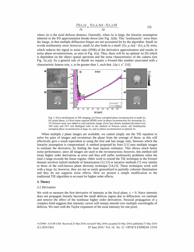
where Δz is the axial defocus distance. Generally, when Δz is large, the linearity assumption inherent to the FD approximation breaks down (see Fig. 1(d)). This „nonlinearity‟ error blurs the image, in that multiple diffraction fringes are not accounted for by the algorithm. Small Δz avoids nonlinearity error; however, small Δz also leads to a small ( , , ) ( , ,0)I x y z I x y term,

which reduces the signal to noise ratio (SNR) of the derivative approximation and results in noisy phase reconstructions, as seen in Fig. 1(a). Thus, there will be an optimal Δz [9] which is dependent on the object spatial spectrum and the noise characteristics of the camera (see Fig. 1(c,e)). As a general rule of thumb we require a Fresnel-like number associated with a

characteristic feature size, x, to be greater than 1, such that 2z x [10].

Fig. 1. Error mechanisms in TIE imaging. (a) Noise corrupted phase reconstruction at small Δz, (b) actual phase, (c) Root mean squared (RMS) error in phase reconstruction for increasing Δz. 1% Poisson noise was added to each intensity image. Error bars denote standard deviation over 100 trials and FFT and Multigrid refer to the method of Poisson solver. (d) Nonlinearity corrupted phase reconstruction at large Δz, and (e) phase reconstruction at optimal Δz.

When multiple z plane images are available, we cannot simply use the TIE equation to solve for pairs of images and reconstruct the phase from the average of those, as this will effectively give a result equivalent to using the first and last image only, between which the linearity assumption is compromised. A method proposed by Soto [11] uses multiple images to estimate the derivative, by finding the least squares estimator. This allows much better noise performance, since all images are used in the reconstruction; however, this method still treats higher order derivatives as error and thus will suffer nonlinearity problems when the total z range exceeds the linear regime. Other work to extend the TIE technique to the Fresnel domain involves hybrid methods of linearization [12,13] or iterative methods [7] very similar to those of the well-known phase diversity technique [14,15]. These techniques work well with a large Δz; however, they are not as easily generalized to partially coherent illumination and they do not suppress noise effects. Here we present a simple modification to the traditional TIE algorithm to account for higher order effects.

3. Theory

3.1 Derivation

We wish to measure the first derivative of intensity at the focal plane, z = 0. Since intensity does not propagate linearly beyond the small defocus region due to diffraction, we estimate and remove the effect of the nonlinear higher order derivatives. Paraxial propagation of a complex-field suggests that intensity curves will remain smooth over multiple wavelengths of defocus. We start with the Taylor expansion of the axial intensity for one pixel,


2 2 3 3 4 4

2 3 4

( ) ( ) ( )( ) (0) ...

1! 2! 3! 4!

z I z I z I z II z I

z z z z

(4)

Here, I(0) is the intensity at focus (due to absorption or non-uniform illumination) and /I z is the desired intensity derivative, which will lead to the phase solution via Eq. (1).

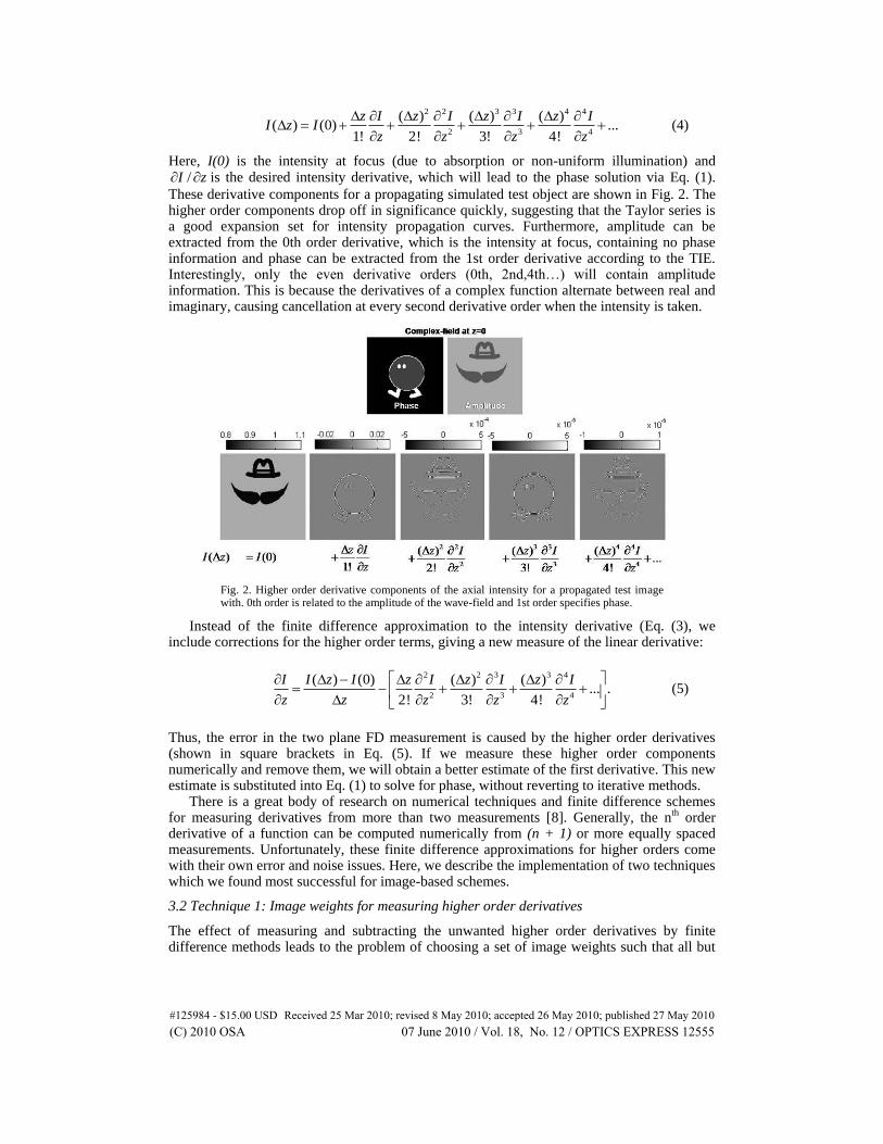
These derivative components for a propagating simulated test object are shown in Fig. 2. The higher order components drop off in significance quickly, suggesting that the Taylor series is a good expansion set for intensity propagation curves. Furthermore, amplitude can be extracted from the 0th order derivative, which is the intensity at focus, containing no phase information and phase can be extracted from the 1st order derivative according to the TIE. Interestingly, only the even derivative orders (0th, 2nd,4th…) will contain amplitude information. This is because the derivatives of a complex function alternate between real and imaginary, causing cancellation at every second derivative order when the intensity is taken.

Fig. 2. Higher order derivative components of the axial intensity for a propagated test image with. 0th order is related to the amplitude of the wave-field and 1st order specifies phase.

Instead of the finite difference approximation to the intensity derivative (Eq. (3), we include corrections for the higher order terms, giving a new measure of the linear derivative:

2 2 3 3 4

2 3 4

( ) (0) ( ) ( )... .

2! 3! 4!

I I z I z I z I z I

z z z z z

(5)

Thus, the error in the two plane FD measurement is caused by the higher order derivatives (shown in square brackets in Eq. (5). If we measure these higher order components numerically and remove them, we will obtain a better estimate of the first derivative. This new estimate is substituted into Eq. (1) to solve for phase, without reverting to iterative methods.

There is a great body of research on numerical techniques and finite difference schemes for measuring derivatives from more than two measurements [8]. Generally, the nth order derivative of a function can be computed numerically from (n + 1) or more equally spaced measurements. Unfortunately, these finite difference approximations for higher orders come with their own error and noise issues. Here, we describe the implementation of two techniques which we found most successful for image-based schemes.

3.2 Technique 1: Image weights for measuring higher order derivatives

The effect of measuring and subtracting the unwanted higher order derivatives by finite difference methods leads to the problem of choosing a set of image weights such that all but


the 1st order in Eq. (5) is cancelled. Consider the linear derivative that we wish to estimate as a superposition of weighted images:

( 1) ( 1) 1 1... ...

,m m m m j j n n n na I a I a I a I a II

z z

(6)

where aj is the image weighting, Ij is the intensity image taken at z = jΔz, meaning I0 is the focused image, negative j corresponds to underfocused images, and positive j corresponds to overfocused images. Thus, (m + n + 1) is the total number of image steps. We seek to find coefficients for each image such that the desired orders are cancelled. This leads to a set of requirements that must be met in order to expect accuracy of a certain order, as given in Table 1. As expected, cancelling higher order derivatives requires more images in order to simultaneously meet all of the desired requirements. The equation to be solved for meeting these conditions is given by:

0 0 0 0

1 1 1 11

2 2 2 22

0( ) ( 1) ( 1)

1( ) ( 1) ( 1)

,0( ) ( 1) ( 1)

0( ) ( 1)

m

m

m

m n m n m nn

am m n n

am m n n

am m n n

am m n

(7)

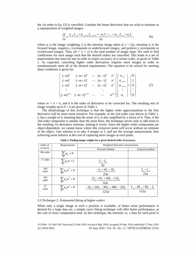
where m + n = k, and k is the order of derivative to be corrected for. The resulting sets of image weights up to k = 4 are given in Table 1.

The disadvantage of this technique is that the higher order approximations to the first derivative will be more noise sensitive. For example, in the 2nd order case shown in Table 1, I1 has a weight of 4, meaning that the noise of I1 is also amplified by a factor of 4. Thus, if the 2nd order component is smaller than the noise floor, the technique serves only to add noise to the resulting 1st derivative estimate, making it worse. Since the higher order components are object-dependent, we cannot know where this crossover point will occur without an estimate of the object. One solution is to take 4 images at I1 and use the average measurement, thus achieving noise balance at the cost of capturing more images at each plane.

Table 1. Finding image weights for a given desired order of accuracy.

Order of accuracy

Requirements Weighted derivative measurement

Forward method Centered method 0th order 0n

N

a

1st order 1n

N

a n 1 0I I

z

2nd order

20n

N

a n 2 1 04 3

2

I I I

z

1 1

2

I I

z

3rd order

30n

N

a n 3 2 1 02 9 18 11

6

I I I I

z

4th order

4 0n

N

a n 4 3 2 1 03 16 36 48 25

12

I I I I I

z

2 1 1 28 8

12

I I I I

z

3.3 Technique 2: Polynomial fitting of higher orders

When only a single image at each z position is available, or better noise performance is desired for a large data set, a simple curve fitting technique will offer better performance, at the cost of more computation time. In this technique, the intensity vs. z data for each pixel is


fit to a polynomial model, and then the desired first order component is extracted for computing phase. In the limit of first order, this technique will be similar to that of [11]; however, by fitting to higher order polynomials, we can obtain a more accurate estimate of the first order derivative. Here we use a least-squares fit to polynomials, which weights all images equally. The order of the polynomial fit function should be less than the number of images used, and more images will result in better noise performance, without sacrificing accuracy. Computationally, each pixel may be treated independently, and fit to a polynomial by standard fitting techniques (least-squares curve fit). The pixelwise treatment lends itself well to parallel computing, such as computation on a Graphics Processing Unit (GPU).

4. Simulations

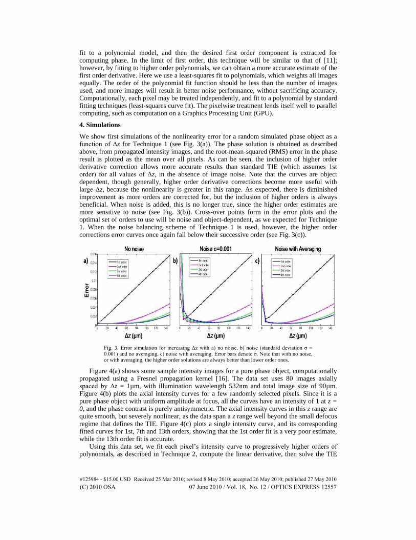
We show first simulations of the nonlinearity error for a random simulated phase object as a function of Δz for Technique 1 (see Fig. 3(a)). The phase solution is obtained as described above, from propagated intensity images, and the root-mean-squared (RMS) error in the phase result is plotted as the mean over all pixels. As can be seen, the inclusion of higher order derivative correction allows more accurate results than standard TIE (which assumes 1st order) for all values of Δz, in the absence of image noise. Note that the curves are object dependent, though generally, higher order derivative corrections become more useful with large Δz, because the nonlinearity is greater in this range. As expected, there is diminished improvement as more orders are corrected for, but the inclusion of higher orders is always beneficial. When noise is added, this is no longer true, since the higher order estimates are more sensitive to noise (see Fig. 3(b)). Cross-over points form in the error plots and the optimal set of orders to use will be noise and object-dependent, as we expected for Technique 1. When the noise balancing scheme of Technique 1 is used, however, the higher order corrections error curves once again fall below their successive order (see Fig. 3(c)).

Fig. 3. Error simulation for increasing Δz with a) no noise, b) noise (standard deviation σ = 0.001) and no averaging, c) noise with averaging. Error bars denote σ. Note that with no noise, or with averaging, the higher order solutions are always better than lower order ones.

Figure 4(a) shows some sample intensity images for a pure phase object, computationally propagated using a Fresnel propagation kernel [16]. The data set uses 80 images axially spaced by Δz = 1µm, with illumination wavelength 532nm and total image size of 90µm. Figure 4(b) plots the axial intensity curves for a few randomly selected pixels. Since it is a pure phase object with uniform amplitude at focus, all the curves have an intensity of 1 at z = 0, and the phase contrast is purely antisymmetric. The axial intensity curves in this z range are quite smooth, but severely nonlinear, as the data span a z range well beyond the small defocus regime that defines the TIE. Figure 4(c) plots a single intensity curve, and its corresponding fitted curves for 1st, 7th and 13th orders, showing that the 1st order fit is a very poor estimate, while the 13th order fit is accurate.

Using this data set, we fit each pixel‟s intensity curve to progressively higher orders of polynomials, as described in Technique 2, compute the linear derivative, then solve the TIE


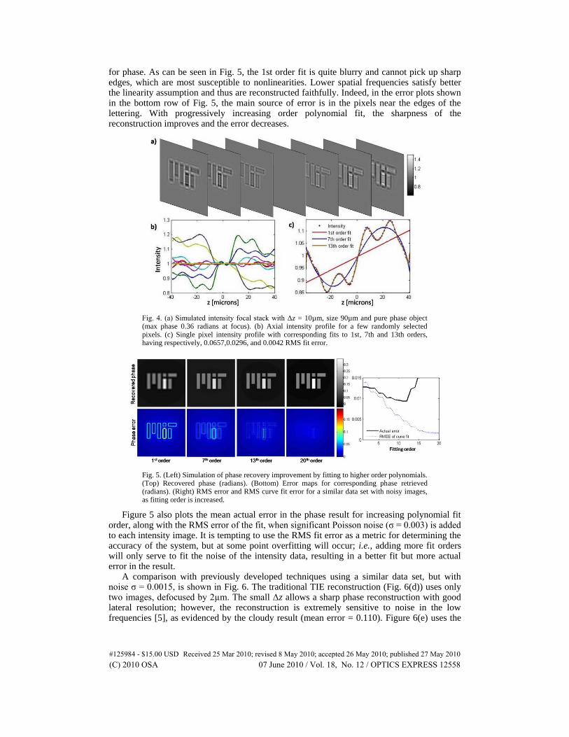
for phase. As can be seen in Fig. 5, the 1st order fit is quite blurry and cannot pick up sharp edges, which are most susceptible to nonlinearities. Lower spatial frequencies satisfy better the linearity assumption and thus are reconstructed faithfully. Indeed, in the error plots shown in the bottom row of Fig. 5, the main source of error is in the pixels near the edges of the lettering. With progressively increasing order polynomial fit, the sharpness of the reconstruction improves and the error decreases.

Fig. 4. (a) Simulated intensity focal stack with Δz = 10µm, size 90µm and pure phase object (max phase 0.36 radians at focus). (b) Axial intensity profile for a few randomly selected pixels. (c) Single pixel intensity profile with corresponding fits to 1st, 7th and 13th orders, having respectively, 0.0657,0.0296, and 0.0042 RMS fit error.

Fig. 5. (Left) Simulation of phase recovery improvement by fitting to higher order polynomials. (Top) Recovered phase (radians). (Bottom) Error maps for corresponding phase retrieved (radians). (Right) RMS error and RMS curve fit error for a similar data set with noisy images, as fitting order is increased.

Figure 5 also plots the mean actual error in the phase result for increasing polynomial fit order, along with the RMS error of the fit, when significant Poisson noise (σ = 0.003) is added to each intensity image. It is tempting to use the RMS fit error as a metric for determining the accuracy of the system, but at some point overfitting will occur; i.e., adding more fit orders will only serve to fit the noise of the intensity data, resulting in a better fit but more actual error in the result.

A comparison with previously developed techniques using a similar data set, but with noise σ = 0.0015, is shown in Fig. 6. The traditional TIE reconstruction (Fig. 6(d)) uses only two images, defocused by 2µm. The small Δz allows a sharp phase reconstruction with good lateral resolution; however, the reconstruction is extremely sensitive to noise in the low frequencies [5], as evidenced by the cloudy result (mean error = 0.110). Figure 6(e) uses the


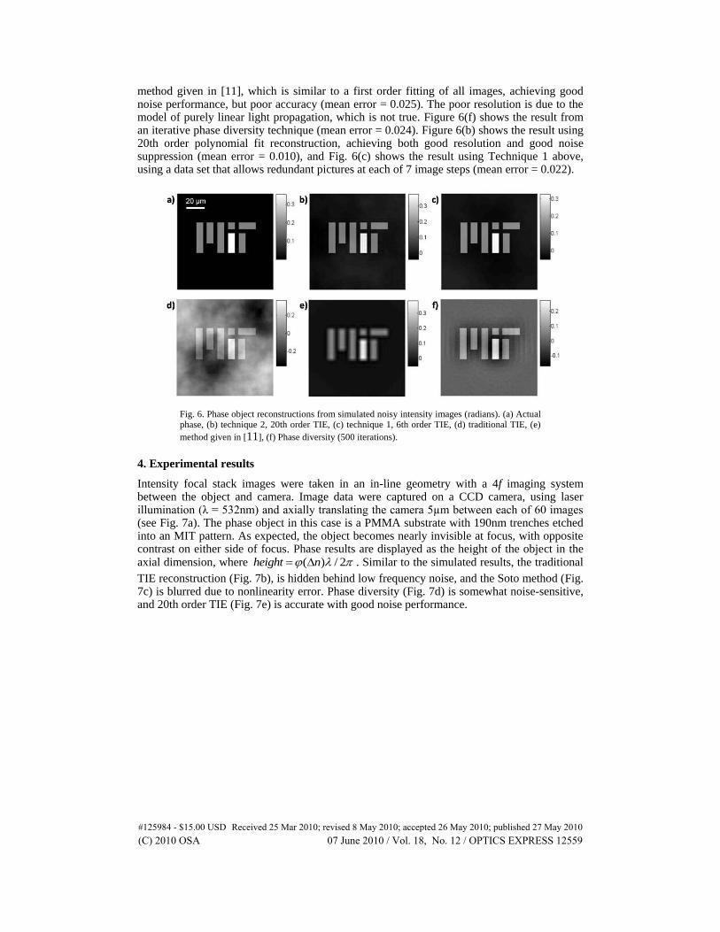
method given in [11], which is similar to a first order fitting of all images, achieving good noise performance, but poor accuracy (mean error = 0.025). The poor resolution is due to the model of purely linear light propagation, which is not true. Figure 6(f) shows the result from an iterative phase diversity technique (mean error = 0.024). Figure 6(b) shows the result using 20th order polynomial fit reconstruction, achieving both good resolution and good noise suppression (mean error = 0.010), and Fig. 6(c) shows the result using Technique 1 above, using a data set that allows redundant pictures at each of 7 image steps (mean error = 0.022).

Fig. 6. Phase object reconstructions from simulated noisy intensity images (radians). (a) Actual phase, (b) technique 2, 20th order TIE, (c) technique 1, 6th order TIE, (d) traditional TIE, (e)

method given in [11], (f) Phase diversity (500 iterations).

4. Experimental results

Intensity focal stack images were taken in an in-line geometry with a 4f imaging system between the object and camera. Image data were captured on a CCD camera, using laser illumination (λ = 532nm) and axially translating the camera 5µm between each of 60 images (see Fig. 7a). The phase object in this case is a PMMA substrate with 190nm trenches etched into an MIT pattern. As expected, the object becomes nearly invisible at focus, with opposite contrast on either side of focus. Phase results are displayed as the height of the object in the axial dimension, where ( ) / 2height n . Similar to the simulated results, the traditional

TIE reconstruction (Fig. 7b), is hidden behind low frequency noise, and the Soto method (Fig. 7c) is blurred due to nonlinearity error. Phase diversity (Fig. 7d) is somewhat noise-sensitive, and 20th order TIE (Fig. 7e) is accurate with good noise performance.


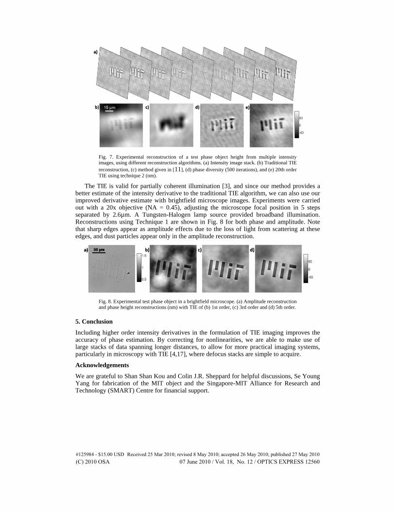
Fig. 7. Experimental reconstruction of a test phase object height from multiple intensity images, using different reconstruction algorithms. (a) Intensity image stack. (b) Traditional TIE

reconstruction, (c) method given in [11], (d) phase diversity (500 iterations), and (e) 20th order

TIE using technique 2 (nm).

The TIE is valid for partially coherent illumination [3], and since our method provides a better estimate of the intensity derivative to the traditional TIE algorithm, we can also use our improved derivative estimate with brightfield microscope images. Experiments were carried out with a 20x objective (NA = 0.45), adjusting the microscope focal position in 5 steps separated by 2.6µm. A Tungsten-Halogen lamp source provided broadband illumination. Reconstructions using Technique 1 are shown in Fig. 8 for both phase and amplitude. Note that sharp edges appear as amplitude effects due to the loss of light from scattering at these edges, and dust particles appear only in the amplitude reconstruction.

Fig. 8. Experimental test phase object in a brightfield microscope. (a) Amplitude reconstruction and phase height reconstructions (nm) with TIE of (b) 1st order, (c) 3rd order and (d) 5th order.

5. Conclusion

Including higher order intensity derivatives in the formulation of TIE imaging improves the accuracy of phase estimation. By correcting for nonlinearities, we are able to make use of large stacks of data spanning longer distances, to allow for more practical imaging systems, particularly in microscopy with TIE [4,17], where defocus stacks are simple to acquire.

Acknowledgements

We are grateful to Shan Shan Kou and Colin J.R. Sheppard for helpful discussions, Se Young Yang for fabrication of the MIT object and the Singapore-MIT Alliance for Research and Technology (SMART) Centre for financial support.



Documents

Transport of Intensity imaging with higher order derivatives