Embed Size (px)
Citation preview

Traffic management Strategies for Merge Areas in Rural Interstate Work Zones1
TRAFFIC MANAGEMENT STRATEGIES FOR MERGEAREAS IN RURAL INTERSTATE WORK ZONES
Prepared for theIowa Department of Transportation
800 Lincoln WayAmes, Iowa 50010
Prepared under theIowa Department of Transportation Management Agreement with Iowa State University
And for theMid-America Transportation Center
University of Nebraska LincolnW333.2 Nebraska Hall
Lincoln, NE 68588-0530
Prepared byT.H. Maze, Director and Professor,
Steve Dale Schrock, Graduate Research Assistant, andKera Sue VanDerHorst, Graduate Research Assistant
Center for Transportation Research and Education2901 South Loop Drive, Suite 3100
Iowa State UniversityAmes, Iowa 50010
July, 1999

EXECUTIVE SUMMARY
The Iowa Department of Transportation, like many other state transportation agencies, isexperiencing growing congestion and traffic delays in work zones on rural interstate highways.The congestion results in unproductive and wasteful delays for both motorists and commercialvehicles. It also results in hazardous conditions where vehicle stopped in queues on ruralinterstate highways are being approached by vehicles upstream at very high speeds. The delaysalso results in driver frustration making some drivers willing to take unsafe risks in an effort tobypass delays. To reduce the safety hazards and unproductive delays of congested ruralinterstate work zones, the Iowa Department of Transportation would like to improve its trafficmanagement strategies at these locations.
To apply better management practices requires knowledge of the traffic flow propertiesand driver behavior in and around the work zone, and knowledge of possible managementstrategies. The project reported here and in a companion report documents research which seeksto better understand traffic flow behavior at rural interstate highway work zones and to estimatethe traffic carrying capacity of work zones lane closure. In addition, this document also reportson technology available to better manage traffic in and around work zone.
Traffic performance data were collected at an Iowa interstate highway work zone usingtraffic data collection trailers. These trailers were constructed as part of this projects and arejointly owned by the Iowa Department of Transportation and the Center for TransportationResearch and Education. They use a pneumatic mast to hoist video cameras 30 feet above thepavement’s surface, to collect video of traffic operations. Videos are then turned into trafficflow performance data using image processing technology.
Through the use of the data collection trailers, traffic performance data were collected atone work zone on Interstate Highway 80 where two lanes are reduced to one lane. Through theanalysis of these data, a work zone lane closure capacity of 1,374 to 1,630 passenger carsequivalents per hour was estimated.
The companion report to this report documents the development of a work zonesimulation model with an animation interface. The simulation model provides a platform for theanalysis of traffic behavior in the merge area and the analysis of delays under varying trafficdemands.
Traffic Management Strategies for Merge Areas in Rural Interstate Work Zones

ACKNOWLEDGMENTS
The project reported in this report was funded, in part, by financial support of the IowaDepartment of Transportation through its management agreement with Iowa State University.Parts of the project were also supported by the Mid-America Transportation Center at theUniversity of Nebraska-Lincoln. We very much appreciate the opportunity to conduct theresearch reported. We are also grateful for the advice and assistance provided by the members ofthe project’s technical advisory committee at the Iowa Department of Transportation. Thecommittee includes Dan Sprengeler, Steve Gent, Mark Bortle, and Dan Houston. In addition, wevery much appreciate the technical advice we were given by members of the staff of theMid-American Transportation Center who help in the development of our data collection trailersand in data collection procedures.
Traffic Management Strategies for Merge Areas in Rural Interstate Work Zones

TABLE OF CONTENTSPAGE
65REFERENCES . . . . . . . . . . . . . . . . . . . . . . . . . . . . . . . . . . . . . . . . . . . . . . . . . . . . . . . . . . . .62WORK ZONE DELAY COST IMPOSED ON MOTORISTS . . . . . . . . . . . . . . .61WORK ZONE CAPACITY . . . . . . . . . . . . . . . . . . . . . . . . . . . . . . . . . . . . . . . . . . . .61CHAPTER 7: CONCLUSIONS AND RECOMMENDATIONS . . . . . . . . . . . . . . . . . . . .57Behavior of the Upstream End of the Queues . . . . . . . . . . . . . . . . . . . . . . .53QUEUE LENGTH . . . . . . . . . . . . . . . . . . . . . . . . . . . . . . . . . . . . . . . . . . . . . . . . . . .49Determining Capacity . . . . . . . . . . . . . . . . . . . . . . . . . . . . . . . . . . . . . . . . . . .49CAPACITY . . . . . . . . . . . . . . . . . . . . . . . . . . . . . . . . . . . . . . . . . . . . . . . . . . . . . . . . .49CHAPTER 6: ANALYSIS AND RESULTS . . . . . . . . . . . . . . . . . . . . . . . . . . . . . . . . . . . . .46SUMMARY . . . . . . . . . . . . . . . . . . . . . . . . . . . . . . . . . . . . . . . . . . . . . . . . . . . . . . . . .45 AUTOSCOPE DATA REDUCTION . . . . . . . . . . . . . . . . . . . . . . . . . . . . . . . . . . . .45CHAPTER 5: LABORATORY DATA REDUCTION . . . . . . . . . . . . . . . . . . . . . . . . . . . .43SUMMARY . . . . . . . . . . . . . . . . . . . . . . . . . . . . . . . . . . . . . . . . . . . . . . . . . . . . . . . . .42Limitations of Data Collection at the Davenport Location . . . . . . . . . . . . .41RESULTS OF SUMMER DATA COLLECTION . . . . . . . . . . . . . . . . . . . . . . . . .40Queue Length Data Collection . . . . . . . . . . . . . . . . . . . . . . . . . . . . . . . . . . . .38Traffic Video Collection . . . . . . . . . . . . . . . . . . . . . . . . . . . . . . . . . . . . . . . . .38FIELD DATA COLLECTION METHODOLOGY . . . . . . . . . . . . . . . . . . . . . . . .37CHAPTER 4: MOBILE TRAFFIC DATA COLLECTION OPERATIONS . . . . . . . . . .33SUMMARY . . . . . . . . . . . . . . . . . . . . . . . . . . . . . . . . . . . . . . . . . . . . . . . . . . . . . . . . .32SELECTION OF SITE CRITERIA . . . . . . . . . . . . . . . . . . . . . . . . . . . . . . . . . . . . .32CRITERIA FOR A SUITABLE LOCATION . . . . . . . . . . . . . . . . . . . . . . . . . . . . .31CHAPTER 3: SITE SELECTION . . . . . . . . . . . . . . . . . . . . . . . . . . . . . . . . . . . . . . . . . . . .28CHAPTER CONCLUSIONS . . . . . . . . . . . . . . . . . . . . . . . . . . . . . . . . . . . . . . . . . . .25Since Function ITS Work Zone Related Systems . . . . . . . . . . . . . . . . . . . .24Traffic Management System in the Region of the Work Zone . . . . . . . . . .23Regional, Statewide, and Multistate Systems . . . . . . . . . . . . . . . . . . . . . . . .21INNOVATIVE WORK ZONE APPLICATIONS OF TECHNOLOGY . . . . . . .18What Do Other State Departments of Transportation Do? . . . . . . . . . . . .17ESTIMATING CAPACITY OF INTERSTATE LANE CLOSURES . . . . . . . . . .12Queuing Behavior . . . . . . . . . . . . . . . . . . . . . . . . . . . . . . . . . . . . . . . . . . . . . .5CAPACITY, FLOW, AND DELAY . . . . . . . . . . . . . . . . . . . . . . . . . . . . . . . . . . . . . .5CHAPTER 2: LITERATURE REVIEW . . . . . . . . . . . . . . . . . . . . . . . . . . . . . . . . . . . . . . . .3PHASE 4: WORK ZONE SIMULATION TOOL . . . . . . . . . . . . . . . . . . . . . . . . . . .3PHASE 3: DATA ANALYSIS . . . . . . . . . . . . . . . . . . . . . . . . . . . . . . . . . . . . . . . . . . .2PHASE 2: DATA COLLECTION . . . . . . . . . . . . . . . . . . . . . . . . . . . . . . . . . . . . . . .2PHASE 1: LITERATURE REVIEW . . . . . . . . . . . . . . . . . . . . . . . . . . . . . . . . . . . . .1CHAPTER 1: INTRODUCTION . . . . . . . . . . . . . . . . . . . . . . . . . . . . . . . . . . . . . . . . . . . . . .
iiiACKNOWLEDGEMENTS . . . . . . . . . . . . . . . . . . . . . . . . . . . . . . . . . . . . . . . . . . . . . . . . . . .iiEXECUTIVE SUMMARY . . . . . . . . . . . . . . . . . . . . . . . . . . . . . . . . . . . . . . . . . . . . . . . . . . .
Traffic Management Strategies for Merge Areas in Rural Interstate Work Zones

TABLE OF TABLES
57Table 6-5 Economic User Delay Costs forObserved Queues . . . . . . . . . . . . . . . . . . . . . . . . . . . . . . . . . . . . . . . . . . . . . . . . . . . . . . .
53
Table 6-4 Observed TrafficCharacteristics Under QueuedConditions . . . . . . . . . . . . . . . . . . . . . . . . . . . . . . . . . . . . . . . . . . . . . . . . . . . . . . . . . . . . .
53Table 6-3 Observed Capacity Valuesduring Free-flow Conditions . . . . . . . . . . . . . . . . . . . . . . . . . . . . . . . . . . . . . . . . . . . . . .
49Table 6-2 Observed Unconverted TrafficPercentages . . . . . . . . . . . . . . . . . . . . . . . . . . . . . . . . . . . . . . . . . . . . . . . . . . . . . . . . . . . .
49Table 6-1 Observed Unconverted TrafficVolumes . . . . . . . . . . . . . . . . . . . . . . . . . . . . . . . . . . . . . . . . . . . . . . . . . . . . . . . . . . . . . . .
42Table 4-2 Summary of Data CollectionDates and Locations . . . . . . . . . . . . . . . . . . . . . . . . . . . . . . . . . . . . . . . . . . . . . . . . . . . . .
37Table 4-1 Field Data Collection TrailerComponent Parts . . . . . . . . . . . . . . . . . . . . . . . . . . . . . . . . . . . . . . . . . . . . . . . . . . . . . . .
35Table 3-4 Suitable Data Collection Sites . . . . . . . . . . . . . . . . . . . . . . . . . . . . . . . . . . . . .35
Table 3-3 Reasons for Elimination ofPotential Data Collection Sites . . . . . . . . . . . . . . . . . . . . . . . . . . . . . . . . . . . . . . . . . . . . .
34Table 3-2 1998 Merge Area StudyCandidate Projects . . . . . . . . . . . . . . . . . . . . . . . . . . . . . . . . . . . . . . . . . . . . . . . . . . . . . .
32Table 3-1 Criteria for a Suitable DataCollection Site . . . . . . . . . . . . . . . . . . . . . . . . . . . . . . . . . . . . . . . . . . . . . . . . . . . . . . . . . .
20Table 2-1 Results of State TransportationAgency Interviews . . . . . . . . . . . . . . . . . . . . . . . . . . . . . . . . . . . . . . . . . . . . . . . . . . . . . . .
Traffic Management Strategies for Merge Areas in Rural Interstate Work Zones

TABLE OF FIGURES
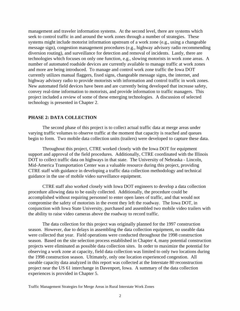
62Figure 7-1, Using Capacity Values to Determine if Congestion Might Occur . . . . . .59Figure 6-12, Speed Change of End of Queue, 8/7/98 . . . . . . . . . . . . . . . . . . . . . . . . . . .59Figure 6-11, Speed Change of End of Queue, 7/10/98 . . . . . . . . . . . . . . . . . . . . . . . . . .58Figure 6-10, Speed Change of End of Queue, 7/02/98 . . . . . . . . . . . . . . . . . . . . . . . . . .58Figure 6-9, Speed Change of End of Queue, 6/19/98 . . . . . . . . . . . . . . . . . . . . . . . . . . .55Figure 6-8, Queue Length on 8/7/98 . . . . . . . . . . . . . . . . . . . . . . . . . . . . . . . . . . . . . . . .55Figure 6-7, Queue Length on 7/10/98 . . . . . . . . . . . . . . . . . . . . . . . . . . . . . . . . . . . . . . .54Figure 6-6, Queue Length on 7/2/98 . . . . . . . . . . . . . . . . . . . . . . . . . . . . . . . . . . . . . . . .54Figure 6-5, Queue Length on 6/19/98 . . . . . . . . . . . . . . . . . . . . . . . . . . . . . . . . . . . . . . .52Figure 6-4, Traffic Volumes and Speeds, 6/19/98 . . . . . . . . . . . . . . . . . . . . . . . . . . . . .52Figure 6-3, Traffic Volumes and Speeds, 8/7/98 . . . . . . . . . . . . . . . . . . . . . . . . . . . . . .51Figure 6-2, Analysis of Ten Highest Converted Free Flow Values, 7/10/98 . . . . . . . .51Figure 6-1, Analysis of Ten Highest Converted Free Flow Values, 7/2/98 . . . . . . . . .47Figure 5-2, Example of Virtual Detectors Placed over Video Image . . . . . . . . . . . . . .46Figure 5-1, Example of Autoscope Supervisor Calibration Grid . . . . . . . . . . . . . . . . .43Figure 4-6, Location of the Data Collection Site at Davenport . . . . . . . . . . . . . . . . . .41Figure 4-5, Example of Collection of Queue-Length Data . . . . . . . . . . . . . . . . . . . . . .41Figure 4-4, Typical Placement of a Calibration Grid . . . . . . . . . . . . . . . . . . . . . . . . . .39Figure 4-3, Typical Location of Field Data Collection Trailer . . . . . . . . . . . . . . . . . . .39Figure 4-2, View of Electronic Equipment in a Data Collection Trailer . . . . . . . . . . .38Figure 4-1, Field Data Collection Trailer in Operation . . . . . . . . . . . . . . . . . . . . . . . .27Figure 2-10, Conceptual Drawing of Indiana Lane Merge System . . . . . . . . . . . . . . .16Figure 2-9, Queue Length Data Collection Schematic . . . . . . . . . . . . . . . . . . . . . . . . .15Figure 2-8, Forward Forming Shockwave . . . . . . . . . . . . . . . . . . . . . . . . . . . . . . . . . . .15Figure 2-7, Backward Forming Shockwave . . . . . . . . . . . . . . . . . . . . . . . . . . . . . . . . . .13Figure 2-6, Example of Deterministic Queueing Theory . . . . . . . . . . . . . . . . . . . . . . .10Figure 2-5, Three Regime Speed-flow Relationship . . . . . . . . . . . . . . . . . . . . . . . . . . .9Figure 2-4, Speed-Flow Relationship Taken From 1985 Highway Capacity Manual . .8Figure 2-3, Speed-Flow Relationship . . . . . . . . . . . . . . . . . . . . . . . . . . . . . . . . . . . . . . . .7Figure 2-2, Flow-Density Relationship . . . . . . . . . . . . . . . . . . . . . . . . . . . . . . . . . . . . . . .7Figure 2-1, Linear Speed Density Relationship . . . . . . . . . . . . . . . . . . . . . . . . . . . . . . . .
Traffic Management Strategies for Merge Areas in Rural Interstate Work Zones

CHAPTER 1: INTRODUCTION
The Iowa Department of Transportation (Iowa DOT) sponsored the Center forTransportation Research and Education (CTRE) conduct of research on the capacity and driver behavior at Interstate work zone merge areas. The principle goal of this research is to determinethe traffic capacity at work zone locations where two lanes of traffic are reduced to one (laneclosure). Reducing two traffic lanes to one in each direction is the typical method of channelingtraffic into a work zone on Iowa's rural Interstate system. When traffic volumes exceed thecapacity of these merge points, the resulting congestion can lead to the formation of queues,which result in delays and increases the potential for traffic crashes. Successful implementationof work zone improvements at locations where congestion is expected will provide a benefit tomotorists through reduced delays and increased safety.
The research project was conducted in four phases: a literature review, the collection oftraffic data at work zone merge areas, the analysis of these data, and the development of acomputer simulation tool to model traffic at merge areas.
PHASE 1: LITERATURE REVIEW
First, a literature review was conducted to determine what research had been previouslyperformed to estimate the traffic-carrying capacity of work zone lane closures and to analyze thebehavior of traffic in work zones. Additionally, other state departments of transportation werecontacted to determine current work zone traffic management methods. This literature reviewand a review of current practices are provided in Chapter 2.
Much of the current body of literature was generated from a number of research projectssponsored by the Texas Department of Transportation (DOT) and conducted by the TexasTransportation Institute during the late 1970s and 1980s. This work is the basis of theprocedures for determining interstate highway work zone capacities used in the HighwayCapacity Manual. In the last two years, there has been renewed interest in this topic and a fewother research projects have recently been conducted on interstate work zone capacity, trafficsafety in work zones, and driver merging behavior. The most significant of these past andongoing projects are ones sponsored by the Indiana and North Carolina Departments ofTransportation (DOTs). Other related projects have been initiated by the Nebraska Departmentof Roads and the state departments of transportation in Iowa (in addition to this project), Kansas,and Missouri.
Another portion of the literature review involved a review of Intelligent TransportationSystems (ITS) that are used to manage traffic in and around work zones and to advise motoristsof work zone-related delays. Applications of ITS generally have two components, the roadsidefield devices and the deskside databases, algorithms and processes used to manage and controltraffic. To date, work zone applications of ITS technology have focused on the roadside andvery little has been conducted to develop deskside procedures and processes. Roadsidetechnology applied to work zones can be broken into three levels. First, there are systems whichmanage traffic and provide motorist information in and around work zones as simply anothertraveler information function of the system. These include regional or statewide traffic
Traffic Management Strategies for Merge Areas in Rural Interstate Work Zones
1
management and traveler information systems. At the second level, there are systems whichseek to control traffic in and around the work zones through a number of strategies. Thesesystems might include motorist information upstream of a work zone (e.g., using a changeablemessage sign), congestion management procedures (e.g., highway advisory radio recommendingdiversion routing), and surveillance for detection and removal of incidents. Lastly, there aretechnologies which focuses on only one function, e.g., slowing motorists in work zone areas. Anumber of automated roadside devices are currently available to manage traffic at work zonesand more are being introduced. To manage and control work zone traffic the Iowa DOTcurrently utilizes manual flaggers, fixed signs, changeable message signs, the internet, andhighway advisory radio to provide motorists with information and control traffic in work zones.New automated field devices have been and are currently being developed that increase safety,convey real-time information to motorists, and provide information to traffic managers. Thisproject included a review of some of these emerging technologies. A discussion of selectedtechnology is presented in Chapter 2.
PHASE 2: DATA COLLECTION
The second phase of this project is to collect actual traffic data at merge areas undervarying traffic volumes to observe traffic at the moment that capacity is reached and queuesbegin to form. Two mobile data collection units (trailers) were developed to capture these data.
Throughout this project, CTRE worked closely with the Iowa DOT for equipmentsupport and approval of the field procedures. Additionally, CTRE coordinated with the IllinoisDOT to collect traffic data on highways in that state. The University of Nebraska - Lincoln,Mid-America Transportation Center was a valuable resource during this project, providingCTRE staff with guidance in developing a traffic data collection methodology and technicalguidance in the use of mobile video surveillance equipment.
CTRE staff also worked closely with Iowa DOT engineers to develop a data collectionprocedure allowing data to be easily collected. Additionally, the procedure could beaccomplished without requiring personnel to enter open lanes of traffic, and that would notcompromise the safety of motorists in the event they left the roadway. The Iowa DOT, inconjunction with Iowa State University, purchased and assembled two mobile video trailers withthe ability to raise video cameras above the roadway to record traffic.
The data collection for this project was originally planned for the 1997 constructionseason. However, due to delays in assembling the data collection equipment, no useable datawere collected that year. Field operations were conducted throughout the 1998 constructionseason. Based on the site selection process established in Chapter 4, many potential constructionprojects were eliminated as possible data collection sites. In order to maximize the potential forobserving a work zone at capacity, field data collection was limited to only two locations duringthe 1998 construction season. Ultimately, only one location experienced congestion. Alluseable capacity data analyzed in this report was collected at the Interstate 80 reconstructionproject near the US 61 interchange in Davenport, Iowa. A summary of the data collectionexperiences is provided in Chapter 5.
Traffic Management Strategies for Merge Areas in Rural Interstate Work Zones
2

PHASE 3: DATA ANALYSIS
After traffic video was recorded in the field, it was brought back to the AutoscopeLaboratory at CTRE to convert the video images to quantifiable data. This process is describedin Chapter 7. The data were analyzed to determine capacity of the work zone merge area. Thesedata are also used to develop estimates of the costs imposed on user through the delays resultingfrom lane closures.
Conclusions and recommendations based on the observed traffic conditions at work zonemerge areas are made in Chapter 8. The range of capacity values of the work zone studied inthis project are presented, along with recommendations on how this range of values could beused by the Iowa DOT to assist in planning the traffic management at future work zones.Insights are drawn concerning the frequency of aggressive motorists. Finally, a recommendationfor improved traffic management planning is offered that may reduce driver frustration duringcongestion at merge areas.
PHASE 4: WORK ZONE SIMULATION TOOL
A computer simulation tool has been developed at CTRE using the ARENA simulationpackage. The purpose of the simulation model is to help Iowa DOT staff better understand
traffic behavior at a work zone lane closure. The simulation package will allow the user to viewtraffic conditions under varying traffic volume levels, and determine estimates of the queue
length and delay. This tool and its supporting documentation is delivered in a companion report.
Traffic Management Strategies for Merge Areas in Rural Interstate Work Zones
3

Traffic Management Strategies for Merge Areas in Rural Interstate Work Zones
4

CHAPTER 2: LITERATURE REVIEW
The purpose of this project was to assist the Iowa DOT in understanding traffic capacitiesof freeway work zone merge points and the resulting motorist delays at various rates of trafficflow. To understand the relationship between one system parameter (capacity) and the other twosystem variables (flow and delay) requires knowledge of the traffic behavior in and around themerge point. To do this, the first part of this chapter introduces the fundamental concepts offacility capacity, traffic flow, and delay. Later, these concepts will be used as a foundation for amore thorough examination of traffic behavior in the work zone. The last part of this chapterexamines advanced technology being applied to better manage traffic and inform drivers oftravel conditions in and around work zones.
CAPACITY, FLOW, AND DELAY
Flow is often referred to as traffic demand. It involves the number of vehicles beingprocessed or arriving to be processed through the merge point per unit of time (usually identified as the variable q). The typical units of flow are in vehicles per hour, vehicle per hour per lane,or passenger car equivalents per hour. Passenger car equivalents take into account the increasedimpact of larger vehicles (in comparison to a passenger car) and the volume of trucks, buses, andrecreational vehicles is factored up to account for their larger impact.
Flow is a function of vehicle density (the number of vehicles per length of road) and thespeed of the traffic flow. Vehicle density is typically noted as the variable k and is reported invehicles per mile or vehicles per lane per mile. Vehicle speed is usually noted as the variable uand is reported in miles per hour. Equation 2-1 is the relationship used to estimate flow. In theflow-density-speed relationship we always refer to the space-mean-speed, as opposed totime-mean-speed. The Highway Capacity Manual defines space-mean-speed as “the averagespeed of the traffic stream computed as the length of the highway segment divided by theaverage travel time of the vehicles to traverse the segment.”(1) The manual definestime-mean-speed as “the arithmetic average of individual vehicle speeds passing a point on aroadway or lane.” The equation used to estimate space-mean-speed is shown in Equation 2-2.Density is the inverse of the vehicle headway (distance from front bumper to front bumper ofconsecutive vehicles) and the equation to estimate the density is in Equation 2-3. Therelationship between flow, density, and speed is expressed below in Equation 2-4.
(2-1)q = nt
(2-2)u =(1/n)
i=1
nli
_t
(2-3)k = n
l
(2-4)q = uk
Traffic Management Strategies for Merge Areas in Rural Interstate Work Zones
5

Where: q = the volume for n vehicles passing a point during time t.
u = the space-mean speed of n vehicles over distance l._t = 1
n [t1(l1 ) + t2(l2 ) + $ $ $ + tn(ln )]k = the density of n vehicles over a distance l.
The terminology for flow on a highway is very similar to the terminology for fluid flow.However, there is one significant difference between the study of the mechanics of most fluidsand traffic. Specifically, most fluids are treated as being incompressible. Because of therelationship expressed in Equation 2-4, both flow and speed are dependent on density which isvery different than the physical relationship for flow of an incompressible fluid.
Bruce Greenshields studied the relationship between flow, speed, and density andpublished his theory on the relationship between the three variables in 1934.(2) Greenshieldspostulated that the relationship between speed and density was linear, as shown in Figure 2-1.Although many have postulated and estimated different functional forms for this relationshipsince Greenshields, the elegance of his original work lies in its simplicity. Shown in Figure 2-1are the freeflow speed ( ) where density is zero, and jam density ( ) where speed decreases touf kjzero. The area under the curve at any point along the curve between jam density and freeflowspeed provides the flow ( ) for that density and speed. The line in Figure 2-1 can be defined byqEquation 2-5. By substituting Equation 2-4 into Equation 2-5, the relationship between flow anddensity is derived and the parabolic flow-density relationship is written in Equation 2-6 andshown in Figure 2-2. In Equation 2-7 is the most commonly cited traffic flow relationship. Therelationship between speed is flow is shown in Figure 2-3.
(2-5)u = uf 1 − kkj
(2-6)q = uf k − k2
kj
(2-7)q = kj u − u2uf
Traffic Management Strategies for Merge Areas in Rural Interstate Work Zones
6

Figure 2-1, Linear Speed Density Relationship
Figure 2-2, Flow-Density Relationship
Traffic Management Strategies for Merge Areas in Rural Interstate Work Zones
7
km
spee
d (m
ph)
Concentration (veh/mi)kj0
0
um
uf
km kj
Flow
(veh
/hr)
0
qm
0Concentration (veh/mi)

Figure 2-3, Speed-Flow Relationship
Greenshields speed-flow relationship (Figure 2-3) has received the most attention and ismost commonly cited in the traffic engineering literature. Prior to the 1994 Highway CapacityManual, the speed-flow relationship based on Greenshields’ model was used as a framework forrepresenting level of service on highways. When a highway is operating at the upper end of thiscurve, motorists are free to maneuver. As the flow increases, the highway becomes morecrowded, individual motorists have less ability to maneuver, and the level of service decreasesuntil the flow reaches the maximum (qm).
Greenshields’ representation of the flow-speed-density relationship is elegant andsimplistic. It uses a single function to represent the entire range of operation (otherwise knownas a single regime relationship). Others have used other functional forms (non-linear equations)to model the speed-flow-density relationship. In Equations 2-8, 2-9, and 2-10, alternative singleregime models developed by Greenberg, Underwood, and Drake, respectively, are shown.(3)(4)(5)
(2-8)u = um lnkj
k
(2-9)u = ume−kkm
(2-10)u = uf e−12
kkm
2
Traffic Management Strategies for Merge Areas in Rural Interstate Work Zones
8
0
0 qm
um
uf
spee
d (m
ph)
Flow (veh/hr)

Where:um = The speed at the maximum flowuf = The mean free-flow speed (speed at low volumes)
Jam density (where flow and speed are zero)kj =/km = The density corresponding to the maximum flow
In the 1960s, researchers began to note that these single regime models did not modeltraffic flow equally well across all levels of traffic density. For example, Greenberg’s modelrepresents behavior better at high traffic densities while Underwood’s model is a betterrepresentation of traffic behavior at lower densities.(6) This illustrates the need for multiple-regime models where different functions are used to represent different portions of thespeed-flow-density continuum.
The conventional thought on speed-flow relationships through the 1985 edition of theHighway Capacity Manual was a single regime curve. The fairly standard relationship betweenspeed and flow is shown Figure 2-4, which is taken from chapter 3 of the 1985 manual. In thelate 1980s and early 1990s research was conducted to analyze this relationship and create a more
realistic model of the speed-flow relationship. Figure 2-4, Speed-Flow Relationship Taken from 1985 Highway Capacity Manual
Hall, Hurdle, and Banks published a paper which identified three distinct portions of thespeed-flow relationship.1(7) A “generalization” of this relationship is shown in Figure 2-5. Theupper portion of the curve (the uncongested portion) is relatively flat. The 1990 interimHighway Capacity Manual first adopted the rather flat upper portion of the curve. The flatnessindicates that speeds diminished very little until the capacity of the facility is reached. The 1994
Traffic Management Strategies for Merge Areas in Rural Interstate Work Zones
9
1 This text is paraphrased from Hall, F.L., “Traffic Stream Characteristics,” Chapter 2 ofUpdate of Traffic Flow Theory, Prepared for the Transportation Research Board Committeeon Traffic Flow Theory and Characteristics.

Highway Capacity Manual fully embraces the relationship of relatively constant speeds whileflow increases in the uncongested portions of the speed-flow. For example, in chapter 3, forfour-lane freeways, the manual shows speed remaining constant until the flow reaches two-thirdsof capacity and speeds only dropping from free flow speed (at 65 miles per hour) to 56 miles perhour at capacity, a reduction in speed of 14 percent as opposed to the 50 percent drop in speedidentified in Greenshields’ relationships. In Figure 2-5, there are really three distinct portions ofthe speed flow relationship; uncongested, queue discharge (free flow recovery and sometimescalled capacity flow), and congested (with queuing). Other researchers have found similarfindings regarding the speed-flow relationship including Banks, Hall, and Hall, Chin and May,Wemple, Morris and May, Agyamang-Duah, and Hall, and Ringert andUrbanik.(8)(9)(10)(11)(12)(13) Findings of all of these researchers support the notion thatspeeds remain fairly constant even at quite high flow rates. Most of the research that has been
done to this point, however, has focused on the shape of the uncongested flow portion of thecurve.(14)
Figure 2-5, Three Regime Speed-flow Relationship
A common aspect of the movement along the curve from uncongested to congested iscapacity drop. In other words, immediately before the flow breakdown occurs the flow rate isgreater than after a flow breakdown. Therefore, when the queuing condition is reached, acapacity reduction (or drop) occurs.(15)(16) The capacity drop is due to turbulence in the trafficflow that results after a breakdown. Later in this report, we present the data we observed at a
Traffic Management Strategies for Merge Areas in Rural Interstate Work Zones
10
Uncongested Flow
Congested Flow
QueueDischarge
Flow
Spe
ed

freeway work zone in Iowa. We did not observe a capacity drop. Although a capacity drop wasnot observed in the Iowa data, a similar study of freeway work zones conducted in NorthCarolina found a precipitous capacity drop. In the North Carolina study, capacity at a laneclosure merge point dropped from 1,210 vehicles per hour to 1,065 vehicle per hour (a 12percent capacity drop) when the traffic arriving exceeds the traffic discharge and flowbreakdown occurred.(17) Other research has found that a capacity drop of approximately sixpercent should be expected once a flow breakdown has occurred and queuing is established. Tothink of this another way, Hall and Agyemang-Duah point out that a six percent “bonus” isavailable if queues can be delayed.(16)
Work conducted in Indiana by Jiang to characterize flow-density relationships atsaturated work zones on interstate highways also found both a speed and a traffic flow dropwhen a queue begins to form at lane closures upstream from work zones.(18) Jiang furthersuggests that after a queue forms, the maximum flow should not be thought of as the capacity ofthe facility. He states that the capacity of the facility should be measured immediately before thequeue forms. After the queue forms, Jiang suggests that the flow rate being observed is reallythe queue-discharge rate, which will usually be smaller than the capacity before a queue forms(due to the drop). Jiang further found that the difference in flow rate between the capacity andthe queue-discharge rate does vary by the type of lane closure. The smallest difference resultswhen there is a lane crossover and discharge flow is being measured for the traffic which crossesthe median (1.6 percent flow rate drop). The flow drop is much greater in the direction that doesnot crossover the median but flows in the opposite direction (20.2 percent drop). When there is aright lane closure and the left lane continues, the flow rate drop is greatest, dropping by 20.9percent. When the left lane is closed and the right lane continues the drop is 9.7 percent. Whatthis suggests is the flow rate bonus of delaying or avoiding a queue (by diverting traffic) can bequite significant and varies with the approach configuration. The difference in the capacity dropfrom a right lane closure and from a left lane closure is due to more traffic having to merge fromright to left rather than the reverse and seeks to illustrate a second point that is inferred fromJiang’s findings. After a queue forms, the capacity is constrained by merging activities upstreamfrom the lane closure taper, where motorists are maneuvering to get into line to enter the workzone. Hence, when the amount of traffic having to change lanes is increased by closing the rightlane and moving traffic onto the left lane, the capacity drop is greatest.
The research conducted in Indiana and North Carolina identify the clear efficiency gainsof keeping an interstate work zone merge area operating on the uncongested portion of the curvein Figure 2-5, above capacity. Further, because of capacity drop, the traffic volumes through thebottle neck required to regain uncongested flow are much lower than the volumes required to gofrom uncongested to congested flow. The difference implies that conditions must be morefavorable (lower flow rate) to regain efficient flow than those required to maintain efficient flow.
In addition to efficiency gains, there are clear safety gains to be enjoyed by not allowinga breakdown on the traffic flow upstream of a work zone merge point. Persaud and Dzbik haveshown that crash frequency clearly increases during congested operation, when compared to thesame faculty during uncongested operation.(19) However, queuing upstream of a work zone ona rural interstate highway presents some unique and hazardous problems for motorists. Tounderstand why this is a more perilous condition requires knowledge of how queues form.
Traffic Management Strategies for Merge Areas in Rural Interstate Work Zones
11

Queuing Behavior
Dixon and Hummer conducted a very thorough study of freeway work zone capacity inNorth Carolina and determined the delays that motorists would experience in work zones.(20) A large portion of their work was devoted to analyzing various models of queuing behavior todetermine the delay motorists could expect at congested facilities. They examined four queuingmodels: deterministic queuing, steady-state stochastic queuing, shock wave analysis, andcoordinate transformation time-dependent techniques (a hybrid mixing both steady-statestochastic queuing and deterministic queuing). Deterministic queuing, steady-state stochasticqueuing theory, and shock wave analysis are described below. Coordinate transformationtime-dependent techniques are not described here because, as Dixon and Hummer discovered,this method does not provide more accurate predictions of queue length than conventionalmodels.
Deterministic Queuing
The most simplistic model of queuing is deterministic queuing. A deterministic model ofqueuing is used by the Highway Capacity Manual to determine delay due to lane closures.Memmott and Dudek applied deterministic queuing at work zones in 1982 and this method isincorporated into the computer model QUEWZ which is used by several state transportationagencies to determine expected delays at work zone lane closures, queue lengths, and usercosts.(21)
The underlying assumption of this model is that when the number of vehicles arrivingexceeds the capacity, the difference between the arrival rate and the capacity is the number ofvehicles stored in the queue. An example of the use of deterministic queuing is shown in Figure2-6. In the Figure it is assumed that the bottleneck has a capacity of 1,400 vehicles per hour.Starting at time zero there is no queue but a queue begins to build because the arrival rate (2,000vehicles per hour (vph)) exceeds the discharge rate (1,400 vhp) and at the end of one hour thereare 600 vehicles queued upstream of the bottleneck. Then the Figure shows the arrival ratedropping to 800 vehicles per hour after one hour at point B. The discharge rate now exceeds thearrival rate and the queue begins to dissipate. At the end of two hours the queue has subsided.The number of vehicle-hours of delay imposed by the bottleneck is the area of the triangleformed by points A, B, and C. Knowing the number of vehicles in the queue, the length of thequeue can be determined by Equation 2-11.
(2-11)Dt =Lt % l
N
Where: Dt = The length of the queue at time t The number of queued vehicles at time Lt = t
l = The average length occupied by a vehicle = The number of lanes upstream from the lane N closure
Traffic Management Strategies for Merge Areas in Rural Interstate Work Zones
12

Time, (hours)1 2
Veh
icle
s, C
umul
ativ
e ov
er T
ime
2,00
02,
800
2,000 vph arrival rate
800 vph arrival rate
1,400 vph queue discharge rate
B
C
A
1,00
0600 vehicles
Figure 2-6 Example of Deterministic Queuing Theory
Dixon, Hummer, and Rouphail point out that the difficulty with the deterministicapproach is that it estimates the queue at a single point.(18) In other words, the model treats thevehicles stored in the queue as if they were stacked vertically rather than distributed across alength of road upstream from the lane closure. Therefore, the behavior of the queued trafficupstream of the lane closure is not influenced by the lane closure.
Steady-State, Stochastic Queuing Model
Steady-state, stochastic queuing models are commonly used for many queuingapplications. For example, they might be used to determine the number of toll booths at a tollplaza required to keep motorist delay below a specified level. The common assumption of astochastic steady state model is that arrivals at the system are random and the service rate (thecapacity) is distributed according to a selected distribution. The assumption of random arrivalrates, particular at high volumes, is not accurate since vehicle headways (interarrival times) aredependent on the other vehicles in the traffic stream. Also, over the analysis period, the arrivalrate cannot exceed the service rate or the steady-state model would project an infinitely longqueue. Having the arriving volume greater than the capacity of the work zone is specifically thecondition that is of interest. As a result steady-state stochastic models are of limited use in theestimation of queue lengths and delay at work zones.
Shock Wave Analysis
Deterministic queuing provides a very simplistic model of queuing by ignoring changesin density of the traffic stream over time and space (cars are assumed to be stacked vertically atthe head of the queue). Lighthill and Whitham developed a shock wave theory whichincorporates variables for both time and space.(22) They postulated that traffic streams are like a
Traffic Management Strategies for Merge Areas in Rural Interstate Work Zones
13

fluid and kinematic waves result from each vehicle. When the number of vehicles arriving at abottleneck exceeds the capacity of the bottleneck, a wave is generated which moves upstream.When the number of vehicles arriving is less than the capacity of the bottleneck the wave movestoward the bottleneck. When the capacity and arrivals are equal, the wave is stationary.
The size and growth of the queue is then dependent on the rate of arriving vehicles, thecapacity of the bottleneck, and the relative density of the arrival stream and the vehicles in thequeue. If the rate of vehicles arriving is Q1 and the capacity of the bottleneck is Q2, where thedensity of arriving vehicles is K1 and the density of vehicles in the queue is K2 , then S inEquation 2-12 is the speed of the shockwave.(23) If S is negative it means that the queue isgrowing and if it is positive it means that the queue is diminishing.
(2-12)S = Q1−Q2K1−K2
Figure 2-7 shows curves for the relationship between flow and density for the bottleneck(the merge point for the lane closure) and highway upstream of the lane closure. The capacity ofthe upstream highway is Qc and the capacity of the bottleneck is Qb. If the flow rate upstream ofthe lane closure is greater than the bottleneck capacity (Qb), then the shockwave is movingupstream (backward moving) at the speed S. A backward moving shockwave is shown in Figure2-7. Figure 2-8 shows a condition where the flow rate upstream of the bottleneck is less than thecapacity of the bottleneck. In this case the queue is dissipating and there is a forward movingshockwave at speed S.
While collecting data in the field, the queue length was measured upstream from thework zone by a vehicle driving on the shoulder of the lane in the opposite direction. The datacollection location of the vehicle and the queue is shown schematically in Figure 2-9. Duringtimes when the queue was experiencing spurts of growth, the driver of the data collection vehiclecould not keep up with the growth of the queue and estimated that it was not uncommon, duringvery short periods of time, for the queue to grow at speeds as high as 30 miles per hour. Thisillustrates one of the dramatic hazards of bottlenecks along a rural freeway. Not only arevehicles approaching a work zone traveling at a high speed but the queue could be growingtoward them at a rate of 30 miles per hour. In other words, a vehicle traveling at 65 miles perhour could in fact be closing with the upstream end of the queue at 95 miles per hour. The actualrate of closure (95 miles per hour) violates the driver’s expected rate of braking and often causeshigh speed rear end crashes.
It is generally accepted that crash rates in work zones are higher than on highway sectionwith similar traffic without work zones. For example, Pal and Sinha studied crash rates atfreeway lane closures and found that there was a statistically significant increase in the crash ratein and around construction lane closures and that the increase was the greatest for lane closureswhere traffic crosses over the median and operates head-to-head on one side of the interstate.(24) In a recent study of crash rates in California interstate highway work zones, Khattak, Khattak,and Council found that in the 36 sites examined, the rate of work zone crashes was 21.5 percenthigher than it was before the locations became a work zone.(25)
Traffic Management Strategies for Merge Areas in Rural Interstate Work Zones
14

Q2
Q1Speed, S
Density (k)
Flow
Rat
e (q
)
k1 k2
Qb
Qc
Q3
Figure 2-7, Backward Forming Shockwave
Q2
Q1
Speed, S
Density (k)
Flow
Rat
e (q
)
K1 K2
Qb
Qc
Q3
Figure 2-8, Forward Forming Shockwave
Traffic Management Strategies for Merge Areas in Rural Interstate Work Zones
15

Data Collection Vehicle. Moves with the upstreamend of the queue, records position over time.
End of queueTo Work Zone
Figure 2-9, Queue Length Data Collection Schematic
Understanding the safety hazard in the queue itself (as opposed to other parts of the workzone) presents some difficulties. To understand the queue’s impact on safety requiresknowledge of the location of the crashes with respect to the location of the lane closure, the typeof crash (rear-end, sideswipe, running into a fixed object, etc.), and the traffic operatingcondition at the time of the crash (free flow or queuing). Unfortunately, these data are notcommonly available.
To collect these very data and to understand the role queuing plays in crashes in andaround workzones, a research project was conducted by the Federal Highway Administration’s(FHWA) Turner Fairbank Laboratory for the National Transportation Safety Board (NTSB).(26) NTSB was particularly interested in crashes 0 to .25 miles, 0.25 to 0.50 miles, and up to 4.0miles upstream of the lane closure.
To satisfy the NTSB requirements, FHWA used two databases. One was supplied by theCalifornia Department of Transportation (CalTrans) and involved 28 multi-lane facility laneclosures in California (17 were on freeways or expressways). The CalTrans database alsoincluded information on the location of the crash with respect to the location of the work zone.The second database was generated by FHWA from crash databases supplied by Minnesota andIllinois. The Minnesota and Illinois databases only provided information which indicatedwhether the crash occurred in the area of a work zone or at other locations along the freeway.The principle use for the Minnesota and Illinois databases are to verify that the California dataare indicative of crash rates in and in advance of work zones lane closures.
The California data are generally found to provide the same characteristics as the basedata from the other two states and the author, therefore, concludes that the California data areindicative of work zone crash patterns elsewhere. Rear-end and sideswipe crashes are found tobe more common at work zones than at other locations, accounting for more than 50 percent ofcrashes in work zones and only 38 percent at non-workzone locations. Rear-end crashes occurTraffic Management Strategies for Merge Areas in Rural Interstate Work Zones
16

when individuals run into the car ahead in the queue and sideswipe crashes occur when anaggressive driver attempts to merge.
Based on the California data, rear-end crashes are occurring about three times asfrequently as sideswipes, both in the work zone and upstream of the work zone. A review ofnational statistics also revealed that rear-end crashes result in a fatality or injury 33 percent ofthe time while sideswipe crashes result in a fatality or injury only 14 percent of the time, thusindicating that rear-end crashes are more hazardous. When the distance of the crash locationupstream from the work zone is examined, it is found that rear-end crashes are more common asyou move upstream. For example, the author found that “on a high-volume facility, rear-endaccidents increase as the distance from the actual work activity increases.” These resultsindicate that stopped vehicles in a queue are more likely to suffer rear-end crashes than motoristselsewhere within the work zone. This finding implies that the possibility of become involved ina rear end crash is only exacerbated by backward-moving shockwaves.
ESTIMATING CAPACITY OF INTERSTATE LANE CLOSURES
Most highway agencies simply use the methods described in the Highway CapacityManual to determine the capacity of a lane closure at an interstate work zone. The capacityestimates in the Highway Capacity Manual are based on the work done at the TexasTransportation Institute by a variety of investigators over a number of years throughout the late1970s and the mid 1980s. This work is based on data collected on Texas Interstate highways bythe Texas Transportation Institute (TTI) and done as part of “Study 292.” Queue and User CostEvaluation of Work Zones (QUEWZ) is a software package used by many state transportationagencies to determine estimated delays, the length of queues, and user costs due to mergers atwork zone lane closures. QUEWZ also originated from the same research program. Later(1987-1991), field data collection was conducted by TTI to update the capacity values and torevise and improve QUEWZ.(27) One of the more significant impacts of the updates was tochange the factor for equating heavy trucks to passenger cars from 1.7 to 1.5. More recently,two studies have been done in North Carolina and in Indiana to try to determine the capacity oflane closures on interstate highways in those states.
Before investigating prior estimates of capacity, it should be recognized that not allestimates of capacity at lane closures are measured using the same criteria. The work done byTTI defined capacity as the hourly traffic volume under congested traffic conditions.(28) TheTTI researchers identified capacity as full-hour volumes counted at lane closures with trafficqueued upstream. They considered consecutive hours at the same location as independentstudies. A Pennsylvania study defined the hourly traffic volume converted from the maximumrecorded five minute flow rate as the work zone capacity. A California study measured volumesfor three-minute time intervals during congested conditions. Two-three minute time intervals,separated by one minute, were then averaged and multiplied by 20 to determine the one-hourcapacity values.(29) Dixon and Hummer define work zone capacity as the flow rate at whichtraffic behavior quickly changes from uncongested conditions to queued conditions.(22) Jiangdefines capacity as the flow just before a sharp speed drop followed by a sustained period of lowvehicle speeds and fluctuating traffic flow which defines the formation of a queue. It is Jiang’s
Traffic Management Strategies for Merge Areas in Rural Interstate Work Zones
17

contention that what TTI was measuring was not capacity of the bottleneck but rather the queuedischarge rate.(20)
TTI work zone capacity research published in 1982 was used as a basis for the methodsfor determining work zone capacity as described in the 1985 Highway Capacity Manual (as wellas the 1994 manual).(27) This work was based on hour-long data collected on urban Texasfreeways with lane closures. The applications of these data may be difficult to extrapolate toother locales due to the difference in driver behavior and differences in design of urban Texasinterstate highway. Texas makes extensive use of frontage roads which makes it much easier formotorists to bypass congested segments of highway. The work conducted by TTI as part ofStudy 292 and work by other institutions and other individuals have resulted in a wealth ofliterature reporting on the measurement of queue discharge rates at work zones under a variety offactors which impact capacity. For example, one study investigated the sensitivity of capacitiesto the use of shoulders during lane closures and to splitting traffic when a center lane isclosed.(30)(31) Some have looked at the type of traffic control devices and their placement andhow they impact capacity and delay. Others have investigated pavement condition, night versusday, traffic volumes and traffic composition, merge discipline and speed control strategies, andthe duration of work zones (short-term versus long-term).(31)(32)(33) Still others haveinvestigated the relationship of the location of construction work to the traffic lane.(30)(34)(22)
The work Dixon and Hummer completed on capacities and delays at work zonesconducted for the North Carolina Department of Transportation in 1996 probably provides themost significant inference for Iowa. The North Carolina study included field data collectedunder conditions similar to those of interest to Iowa: lane closures on two-lane rural interstatehighways. The North Carolina study used a more relevant measure of capacity for a lane closurethan the TTI researchers. The North Carolina researchers defined capacity as the traffic volumeimmediately before queuing begins. An important and unique finding of the North Carolinastudy is the identification of the location within work zone that governs maximum traffic flowthrough the work zone. The location tends to vary with traffic conditions and with constructionwork activities. The work done in Texas by TTI has assumed that the feature governing themaximum traffic flow is the point at the end of the taper. Dixon and Hummer report that themaximum flow is governed by three locations. The maximum flow is controlled by the segmentof the work zone travel path adjacent to the work area where the construction work activity isheavy; meaning large equipment and workers adjacent to the travel path. Under conditionswhere the work activity is low, then the maximum flow (prior to queue formation) is governedby the end of the merge taper. However, when the work activity is heavy, the maximum trafficflow was found to be about seven percent less than the maximum flow at the taper end for workzones on two-lane rural interstate highways. When a queue has formed, the maximum flow isgoverned by the merging activity upstream from the work zone. In other words, once a queuehas been formed, the maximum flow of the entire work zone is governed by the rate at whichtraffic can be discharged from the queue, which is generally at a lower rate than the capacity ofthe taper end, accounting for capacity drop when a queue is formed.
What Do Other State Departments of Transportation Do?
Traffic Management Strategies for Merge Areas in Rural Interstate Work Zones
18

To determine how other state departments of transportation (DOTs) deal with congestionproblems, we conducted telephone interviews of individuals representing 22 state DOTs duringthe summer of 1997. We explained the nature of our research and asked the representatives iftheir agency was experimenting with innovative approaches to manage traffic through interstatework zones, if they have attempted to conduct any strategies to improve the capacity of interstatework zones, or if they have attempted to measure the capacity of interstate work zones. Theresponses we received are listed in Table 1.
North Carolina and Indiana currently are or have recently documented research on workzone capacity analysis, although other states believed that they have conducted research on workzone capacity but failed to document their findings. Texas conducted work zone capacityanalysis and this research forms the basis for the methods described in the Highway CapacityManual. Most states simply use the Highway Capacity Manual’s methodology and theirexperience to evaluate traffic flow and delay in work zones.
Traffic Management Strategies for Merge Areas in Rural Interstate Work Zones
19

Developed their own field manual for traffic control and havefield tested and deployed a work zone management trafficmanagement field device (this is discussed in the technologysection of this literature review). However, no investigation hasbeen conducted into capacity analysis of work zones.
Minnesota DOTBill Servatius, WorkZone Safety Unit
Signing, particularly the location of changeable message signsand arrow panels, has been investigated through their constructionzone advisory committee. Another important issue in Michigan isthe reluctance of police to enforce work zone traffic control. Noresearch has been initiated to manage work zone congestion.
Michigan DOTBruce Monroe, Trafficand Safety Division
Nothing has been conducted to date related to congestion at workzones but will be working with the other states in the region toevaluate new work zone traffic control technology.
Kansas DOTMike Crow, State TrafficEngineer
Jiang has been collecting field data to measure capacities of workzones in Indiana and his findings have been reported in theliterature.(20),(35),(36). Tarko was working on the field testingof a variable no pass zone.
Indiana DOT (referred toPurdue University)Yi Jiang, ResearchAssistant (now with theIndiana DOT) andAndrzej Tarko, Professor
No activityGeorgia DOTMarion Waters, StateTraffic and SafetyEngineer
Working on developing standards for ITS application but nonehave been for work zone related applications. No evaluation ofwork zone traffic capacities.
Florida DOTJeff Morgan, ResearchLaboratory
Currently conducting some speed studies. Believed that theyhave done some capacity analysis in the past but nothing waspublished.
Connecticut DOTWalter Coughlin, TrafficEngineer
Merging at lane closure approaches is a problem, especially inurban areas, but have not tried any new procedures to mitigateproblems.
Colorado DOTMathew Reay, TrafficEngineer
Base capacity estimations on methods presented in the HighwayCapacity Manual.
California DOTDon Fogel, SafetyResearch
No activityArizona DOTMike Manthey, StateTraffic Engineer
CommentsAgency and ContactTable 2-1 Results of State Transportation Agency Interviews
Traffic Management Strategies for Merge Areas in Rural Interstate Work Zones
20

Nothing to reportVirginia DOTDave Rousch, TrafficEngineer
Texas conducted a number of studies in the late 70s, 80s, andearly 90s on work zone capacity analysis and this work has beenthe underpinning of most of the information available nationally.They have done very little recently to incorporate innovativemethods to control congestion in and around work zones.
Texas DOTGreg Brinkmeyer, TrafficEngineering
Believed that there had been studies on work zone capacities butnothing published. Currently negotiating a project with theUniversity of Cincinnati to evaluate a technology which willinform the driver the delay they should expect when travelingthrough an interstate work zone.
Ohio DOTYuanita Elliot, TrafficEngineer
Experimenting with arrow boards and changeable message signsto promote more orderly merge discipline, placement of rumblestrips to promote attention to signs, and a variety of pavementmarkings. Conducted study with North Carolina State Universityto determine capacity of work zones.(21)
North Carolina DOTRobert Cannalis, TrafficEngineer
Experimenting with changeable message signs and planing toexperiment with portable rumble strips. Have not evaluated workzone capacity or congestion management strategies.
New York DOTThomas Werner, Trafficand Safety Division
Working with the University of Nebraska to determine promisingtechnology to better manage congestion in and around freewaywork zone. Will also be evaluating work zone traffic controltechnology with the other states in the region.
Nebraska DORDan Waddle, TrafficEngineer
Nothing has been conducted to date related to congestion at workzones but will be working with the other states in the region toevaluate new work zone traffic control technology.
Missouri DOTTom Borgmeyer, TrafficEngineer
CommentsAgency and ContactTable 2-1 Continued
INNOVATIVE WORK ZONE APPLICATIONS OF TECHNOLOGY
There is a wide variety of novel applications of technology to better manage trafficaround and through work zones. Some focus on productivity improvements (delay reduction)and some focus on safety (e.g., reduction of speeds in work zones); however, to some degree,improvements in safety and improvements in productivity go hand in hand. In other words,applications with a focus on delay reductions improve traffic flow and, therefore, improve trafficsafety.
Applications of technology can vary widely in scope. Some systems, like the Iowa DOTwork zone web page, are statewide in scope and are focused on traveler information to allowindividuals to make better route and/or travel time choices. Generally, these systems focus on avariety of types of traveler information. For example, the Arizona DOT Trailmaster Highway Closure and Restriction System (HCRS) provides information on all conditions which effect
Traffic Management Strategies for Merge Areas in Rural Interstate Work Zones
21

highway travel (e.g., incidents, weather, and congestion), not just roadway construction.(37) The HCRS involves an intranet system which carries information for use by the Arizona DOT tohelp support the management of its system. The system also acts as an extranet and carriesinformation between the Arizona DOT and partner agencies (e.g., counties, state police, etc.),and an internet that provides information to the public. The intranet portion of the system onlyprovides information on the location and type of lane restriction or closures for use by the public,while the other portions of the system, the extranet and intranet, are interactive and allow fortwo-way communication. The public can gain access to the public portion of the informationsystem through the internet, through an automated telephone system, or through kiosks.Although the system provides useful information for the public, the agencies managing thehighway system benefit greatly by having better information on current conditions and activitieson the highway network. The Arizona DOT is working with adjacent states to expand thesystem to areas contiguous with Arizona. A similar system, the Condition Acquisition andReporting System (CARS), is being developed by the Iowa DOT in conjunction with other statesin the region.
In urban areas, highway operating agencies will deploy traffic management systems tomonitor traffic conditions; manage traffic through traveler information and traffic controldevices such as ramp meters; and detect and manage incidents. To the extent that there are alsowork zones on highways under traffic management, they will also manage traffic in and aroundwork zones. However, it is important to draw a distinction between urban highways undermanagement and work zone locations. Typically, even if work zones involve urbanconstruction, any surveillance, detection, and traveler information system must be in temporarylocations (as opposed to permanent locations) due to the need to move field equipment aswarranted by construction activities. For example, the Des Moines early deployment plan callsfor surveillance and video detection cameras to be put in place along the I-235 right-way beforethe facilities reconstruction at temporary locations.(38) Later the same equipment could bepermanently mounted adjacent to I-235 once reconstruction is completed. In rural work zones,where traffic volumes do not warrant permanent surveillance after construction, the ITS fielddevices (detectors, communication systems, changeable message signs, etc.) and any systemsthat are put in place during construction must be capable of being relocated.
Because of the costs involved, statewide or multistate traveler information systems, suchas the public portion of HCRS, operate with very little primary data and utilize data fromsecondary sources (police reports, reports from maintenance crew, reports from field offices,weather service information, etc.). These systems generally provide a variety of information inaddition to work zone congestion and delay information for an entire state or multistate area.The primary intent of high level traveler information systems are to increase efficiency byallowing drivers to make more informed route and/or time of travel choices.
Some ITS applications, which provide work zone related user services, are more localand focus on the management of traffic in the area of the work zone. For example, during thesummer of 1997, the Iowa DOT tested and deployed systems, including highway advisory radio(HAR), incident detection technology, changeable message signs (CMS), and video cameras, “tomonitor approaching traffic speeds and volumes, determine when traffic backups occur, activatethe warning devices, and inform surveillance personnel of the problem.” (39) These systems
Traffic Management Strategies for Merge Areas in Rural Interstate Work Zones
22

manage traffic and incidents in the region of the work zone, focusing on the management ofseveral aspects of the work zone but with a scope limited to a single work zone. Other systems,with features similar to the Iowa systems, have been tested over the last 5 to 6 years and arebeing deployed. A common attribute of all of these systems is that they operate in a reactivemove. In other words, they wait for an incident or congestion to occur and then deploymanagement strategies to deal with the deteriorated condition. No systems were found thatoperate in a proactive mode where forecasts of traffic conditions (based on historical data or timeseries forecast of traffic volumes) and management strategies are deployed in advance to avoidor mitigate congestion.
Still other types of ITS technology are limited to a single function. For example, theOhio DOT has been field-testing equipment which informs drivers of the delay they cancurrently expect when traveling through a work zone upstream of their current location.(40) Once they are informed of the delay, the motorist can choose to divert to an alternative route orcontinue through the work zone. In limited field testing, the Ohio devices have received positiveevaluations in motorist surveys. This type of device is intended to achieve a single mission. Inthe following sections, we briefly discuss technology being currently applied at the statewide andmultistate level, at a multifunction level where traffic is managed in the region of the work zone,and at the single function level.
Regional, Statewide, and Multistate Systems
Traffic management systems and traveler information systems at the metropolitan andstatewide level generally include information on work zones and develop management strategiesto mitigate congestion caused by highway construction or maintenance. These systems,however, tend to have a much broader functionality than just informing travelers of maintenanceor construction related lane restrictions. For Iowa, the issue of traveler information services on astatewide basis will be planned as part of the Iowa ITS Strategic Planning study currently beingconducted (spring and summer, 1999). It is, however, important that the user services forinforming motorists of work zones, likely work zone delays, and recommended diversion routesare accommodated in the statewide system architecture recommended by the consultant.
Although the current state ITS strategic plan will ultimately develop a systemarchitecture for ITS services at the state level, it is important to recognize that travelers andcommercial transportation services do not restrict themselves to political jurisdiction boundaries.An example of a group which has recognized that services must reach beyond state borders is theI-95 corridor coalition. The coalition is a group of 12 states stretching from Maine to Virginiaalong the eastern seaboard. The Information Exchange Network (IEN) created through the I-95corridor coalition seeks to exchange information on traffic conditions, incidents, and plannedevents which restrict highways in the corridor.(41) The network connects major transportationagencies in the corridor and the information is available for agencies to use and prepare fordistribution to travelers. One creative use of the information available through IEN has beendeveloped through an FHWA-sponsored (along with a whole myriad of private and public sectorpartners) operational test titled TruckDesk.(42) The TruckDesk project demonstrated thatinformation from IEN and other public and commercial information services could be processedand delivered to motor carrier dispatchers. This information adds enough value that motor
Traffic Management Strategies for Merge Areas in Rural Interstate Work Zones
23

carriers are willing to pay fees to support the service.(43) As a result, the project has moved to aself-supporting phase and changed its name to FleetForward. This project has been so popularthat other travel information system projects (e.g., San Diego’s Intermodal TransportationManagement Center) are adapting similar services.(44) The value of these systems is proven bythe private sector’s willingness to pay for information services.
Traffic Management Systems in the Region of the Work Zone
Generally, it is the objective of these systems to provide an affordable means ofdelivering traffic management services, like the surveillance provided to an urban faculty underthe management of a Traffic Operations Center (TOC). Typically, instrumenting a work zonewith ITS field devices would not be financially feasible due to the cost of placing the highwayunder the management of a TOC. For example, the Minnesota DOT uses a figure of 500,000dollars as a planning number for placing a mile of interstate highway under the management of aTOC. Because of the expense, transportation agencies have focused on less expensive portabledevices. A few mobile traffic management systems have been developed, tested, and are beingused to manage the traffic in the area of work zones.
They typically involve video surveillance, traffic detection (using video detection orsome other non-intrusive technology), and usually a combination of devices to communicateconditions to the drivers and manage traffic, typically using changeable message signs (CMS)and/or highway advisory radio (HAR). The Minnesota DOT’s ITS office (Gudiestar), with anumber of partners, has developed a field device they have titled the “Smart Work Zone”(SWZ).(45) The SWZ is the second generation device. The first generation device was thePortable Traffic Management System (PTMS) and it was first field tested in 1994.(46) Theobjective of PTMS and SWZ is to provide a traffic manager, located in a remote office, withvideo images and video detection in and around the work zone so that she/he can manage trafficthrough remote controlled CMSs. The communication systems for the system are wireless dueto the difficulty or impossibility of wireline communications in a work zone.
Portable work zone traffic management systems have proven beneficial. For example,the evaluation of SWZ found a significant increase in the traffic volume that traverse urbanfreeway work zones while under the management of the SWZ. In the evaluation of SWZ a 3.6percent increase traffic volumes in the morning peak were found and a 6.6 percent increase in theafternoon peak. In addition, the system decreased the speed variability of vehicles approachingthe work zone and decreased the average approach speed by 9 miles per hour. Other work zonetraffic management systems have been or are being developed elsewhere. For example, TheScientex Corporation has developed a commercially available system called ADAPTIRTM.(47) Another system was developed by Computran Systems Corporation for the New YorkDOT.(48)(49) The Computran system is being developed for a large expressway interchangereconstruction project but has many of the same features as the SWZ.
Single Function ITS Work Zone Related Systems
Traffic Management Strategies for Merge Areas in Rural Interstate Work Zones
24

There have been a number of attempts to develop systems which improve safety or thecapacity of work zone lane mergers. Safety-related devices generally attempt to slow driversapproaching work zones through a number of strategies or protect the workers in the work zonethrough alarms, remote controlled shadow vehicles, automated flaggers, and decoy enforcementvehicles. In this review, we will focus on a few of these devices. Several more are being testedas part of the MidWest States Smart Work Zone Deployment Initiative and more equipment isbeing demonstrated and developed by highway agencies and technology vendors.
Efforts to Improve the Merger Discipline
As defined earlier in this literature review, the constraint imposed on the carryingcapacity of a multi-lane highway due to a work zone lane closure varies with the level of activityin work zone and the condition of traffic flow through the lane closure. When the constructionwork adjacent to the travel lanes is heavy (construction workers and large equipment in closeproximity to the travel lane), then the capacity is governed by the travel lane immediatelyadjacent to the active work area. Where construction is not heavy immediately adjacent to thetravel lane, and prior to traffic volumes reaching saturation (prior to generation of a queue),capacity is governed by the end of the taper at the merge point. Following saturation, capacity isgoverned by merging activities upstream of the merge point. If the merger discipline ofmotorists can be modified to improve the efficiency of merger operations, then, after saturationhas occurred, the work zone traffic throughput can be increased.
The failure of vehicles to merge into the through lane by the end of the queue canpromote frustration on the part of some motorists. In an effort to avoid waiting through a queueat a lane closure, some drivers will continue to travel in the closed lane, merging into the openlane as late as possible. This behavior can be a safety problem because late merging vehiclesmay take risks and accept unsafe gaps to merge. In addition, motorists who have already mergedinto the queue must watch in frustration as the late merging vehicles pass them. To block latemerging vehicles, it is common to observe cars straddling both lanes or truck drivers whocooperate and travel slowly down both lanes side by side, thereby blocking cars proceedingdown the closed lane. Both late merging and vehicles blocking the closed lane tend to reduce thecapacity of the faculty at the merge point. As a result, the Pennsylvania and Indiana DOTs haveattempted to modify driver behavior and improve merge discipline.
The Pennsylvania DOT’s approach is to not encourage motorists to merge upstream fromthe lane closure and instead allow motorists to merge immediately upstream of the taper.(50) Approximately 1.5 miles upstream of the merge point, a sign is posted stating “USE BOTHLANES TO MERGE POINT.” At 350 feet upstream of the taper for the lane closure, a sign tellsmotorists to “MERGE HERE - TAKE YOUR TURN,” thus allowing travel to the merge point inthe closed lane. By allowing travel in the closed lane, the tension between motorists mergingearly and late is minimized.
The Pennsylvania DOT’s late merge program is a low technology approach to improvingcapacity. However, it was felt that it should be described in this section since other hightechnology approaches are being applied to enhance the capacity of the mergers on multi-lane
Traffic Management Strategies for Merge Areas in Rural Interstate Work Zones
25

facilities. They have studied the late merge approach and found that its application increased thecapacity of merging operation by as much as 15 percent.(51)
The benefit of this approach is that signs create a no passing zone which starts before theend of the queue (assuming that the queue never exceeds the distance upstream of the location ofthe last dynamic sign). This should stop aggressive drivers who attempt to bypass the queue bytraveling in the closed lane to the head of the queue. A prototype system was tested in Indiana in1996 and more testing is to be conducted during the summer of 1999.(52) In simulation analysisconducted as part of CTRE research (reported in the companion simulation report), a variable nopass system was evaluated using microscopic simulation. The CTRE simulation model resultsshowed an increase in capacity and an increase in traffic speeds and reduction in delay when thevariable no pass system is applied. However, unlike the actual application of this technology,our simulation model assumes all drivers will obey the signs.
Traffic Management Strategies for Merge Areas in Rural Interstate Work Zones
26

Figure 2-10, Conceptual Drawing of Indiana Lane Merge System (taken from (53)
Speed Reduction Technology
New technologies to reduce speed, speed variations, and the number and speed of highspeed vehicles (above the 85th percentile) are still evolving. Several new technologies will beevaluated as part of the MidWest States Smart Work Zone Deployment Initiative during thesummer of 1999 (a project in which the Iowa, Kansas, and Missouri DOTS and the NebraskaDepartment of Roads are participating). However, here we examine only two existing speedreduction technologies which have had significant evaluation and testing.
One technology is the use of a drone radar device to make drivers with radar detectorsbelieve there are radar-equipped enforcement personnel in the vicinity of the work zone. Thishas the effect of slowing down drivers fearful of being cited for speeding. Several evaluationshave been conducted of this type of device and it has been shown to reduce the average speedand reduce the percentage of high speed vehicles. A study of unmanned radar by Pigman et al.at high crash frequency locations along I-75 in Kentucky found that at one of the two experimentsites, the average speed was reduced by 1.7 miles per hour.(54) Also, the variance of speeds andthe 85th percentile speeds were reduced at both locations. Ullman and Riesland conducted anevaluation of unmanned radar by observing speeds immediately upstream from work zones withdrone radar units at eight sites in Texas.(55) At the seven sites where large speed data sets werecollected, the deployment of the drone radar reduced average speeds from 0.2 miles per hour to1.7 miles per hour. At some of the sites, a greater speed reduction was noted for trucks ascompared to cars and a greater reduction was noted in the speed of high speed vehicles ascompared to the average speed of all vehicles.
Traffic Management Strategies for Merge Areas in Rural Interstate Work Zones
27

In Illinois, Benekohal, et al. evaluated unmanned radar in a work zone for a few hours.They found that within the first few minutes of radar operation, the average speed reduced byalmost 10 miles per hour. However, over a three hour data collection period, there was not astatistically significant reduction in average speed.
A Virginia study of unmanned radar by Turochy and Sivanandan evaluated the system atthree work zones, each with a different configuration.(56) Two were long-term work zones(multi-day construction projects) while the third project was a short-term project, lasting onlyone day. In all three cases, a reduction in average speed was observed although in one case itwas not statistically significant. The average speed reduction observed ranged from 0.8 milesper hour to 2.3 miles per hour. The researchers also observed reductions in the standarddeviation of speed of 0.1 miles per hour to 0.5 miles per hour, a reduction in the traffic exceedingthe speed limit by 6 to 20 percent, and a reduction in the 85th percentile speed of 1.1. miles perhour to 3.9 miles per hour. The authors conclude that unmanned radar is more effective intemporary work zones, presumably because in temporary work zones drivers do not get enoughexposure to the operation to know that there are no enforcement personnel present in the workzone. They also conclude that in work zones where motorists have the expectation thatenforcement officials may be present, the unmanned radar can be just as effective at reducingspeed as having an enforcement personnel present.
Another technology used to reduce speed is the radar speed monitor display. This is adevice which automatically monitors and displays the speed of vehicles passing through thework zone using radar. The objective is to make drivers aware of their speed through digitaldisplay and drivers with radar detectors are likely to believe that their speed is being monitoredby enforcement personnel. The Iowa DOT deployed this technology in the mid 1970s when itmounted a speed monitor and display device over I-35 just south of Ames, Iowa in the southbound lane. Similar devices were used for traffic calming in Berkeley, California, where theyreduced average traffic speed by as much as 20 miles per hour.(57)
McCoy, et al. evaluated the speed monitor display device for the South Dakota DOT in1993. When placed in advance of work zones, these devices were found to be effective andreduced average speeds by four to five miles per hour. In addition, the number of high speedvehicles was reduced. They found that the number of vehicles exceeding the advisory speed bymore than 10 miles per hour was reduced by 40 percent. McCoy, et al. concludes that the speeddisplay system appears to have more beneficial impact than unmanned radar.
CHAPTER CONCLUSIONS
This chapter first presented fundamental principals of traffic flow theory to providereaders with a foundation to assist them in understanding the context of research related to thecapacity of work zone lane closures. Much information on the capacity of work zone laneclosures and delays was developed through research conducted by the Texas TransportationInstitute (TTI) through a series of projects which started in the late 1970s and continued throughthe 1980s. The results of the TTI work are commonly used by transportation agencies and thefindings are the basis of the lane closure capacity analysis reported in the Highway CapacityManual. Only recently has significant additional research been conducted in other locations
Traffic Management Strategies for Merge Areas in Rural Interstate Work Zones
28

(other states) to add to the body of knowledge on work zone lane closure capacity. One of themore important additions to recent research was to provide a clearer definition of the capacity ofwork zone lane closures.
The TTI work defined traffic carrying capacity of a work zone lane closure to be trafficflowing through the work zone under congested conditions. Jaing points out that the volumeunder congested conditions is really the queue discharge traffic flow rate and not the capacity ofthe lane closure.(35) In most cases, the peak flow immediately before saturation is really greaterthan the flow through the system after saturation. Therefore, Jaing defines capacity as thevolume of traffic flowing through work zones immediately before congestion generates a queue.
The phenomenon where both average speed and volume drop after saturation is known ascapacity drop. Because of capacity drop, the traffic volumes through the bottle neck required toregain uncongested flow are much lower than the volumes required to go from uncongested tocongested flow. The difference implies that conditions must be more favorable to regainefficient flow that those required to maintain efficient flow. Thus there is a capacity bonus forkeeping traffic flows below the level where the lane closure becomes saturated.
Our review of work zone-related ITS technology found that ITS applications dealing withwork zone traffic management and traveler information focus at three levels. At the highestlevel, there is traveler information that operates on a region, statewide, or multi-state level.Although providing travelers with information regarding possible delays due to work zones is animportant feature, these systems typically report information for all types of road closures andrestrictions (e.g., restrictions caused by weather or an incident). The next level down are mobilesystems that attempt to manage traffic in the area of the work zone. These utilize a number offield devices (e.g., CMSs, HAR, video surveillance, etc.) in combination with managing traffic.The last level are applications with a single purpose, e.g., reduce the speed of traffic through thework zone, inform drivers of the travel time through the work zone, or improve traffic flow bymodifying the merger discipline. Systems at all three levels tend to be reactive rather thanproactive. Others wait for congestion to build, then assist traffic managers to better manage thecongestion that has already occurred. It appears that there is a great deal of opportunity todevelop systems which are proactive and implement strategies in advance of congestion. Forexample, a system which is capable of predicting when congestion is likely to occur could beused to deploy diversion strategies well in advance and upstream of the lane closure, possiblydelaying or avoiding saturating the lane closure.
Traffic Management Strategies for Merge Areas in Rural Interstate Work Zones
29

Traffic Management Strategies for Merge Areas in Rural Interstate Work Zones
30

CHAPTER 3: SITE SELECTION
CTRE project team personnel met on two occasions with Iowa DOT staff to identifyattractive data collection sites. During the meetings, which were held on April 28 and May 15,1998, a list of essential criteria for an acceptable data collection site was developed and potentialwork zone locations were identified.
CRITERIA FOR A SUITABLE LOCATION
The April 28 meeting included Iowa DOT staff members Mark Bortle, Steve Gent, DanHouston, Dan Sprengler and CTRE’s Dennis Kroeger and Steve Schrock. The objective of themeeting was to determine suitable criteria for an acceptable data collection site.
The DOT staff determined that an ideal location would be a section of interstate wherework zone congestion had occurred in previous years. In general, this included Interstate 80from Des Moines to Davenport, Interstate 35 from Ames to Des Moines, and Interstate 380 fromIowa City to Cedar Rapids. It was also decided to keep the sites rural if possible to reduce theimpact urban commuters have on speed and headways. Urban locations would be used,however, if no other suitable locations could be found.
The types of projects that might provide a suitable merge area at which to collect datawere discussed. The Iowa DOT staff believed that a long-term construction project would beadvantageous because it would provide the duration needed to collect multiple days of data. Itwas also decided to try to use shorter-term construction or maintenance projects if they tookplace within the areas discussed above, but only as an alternative to long-term work zones. Anyproject where the work zone layout would be static for at least one day would be adequate for thepurposes of data collection.
The desired physical attributes of the interstate at a possible data collection site were alsodiscussed. Ideally, locations that were as far as possible from interchanges were desired in orderto minimize the impacts of merging traffic. Also, in order to keep all potential locations roughlyequal, it was decided to only look at merge areas where two lanes of traffic were reduced to one.This would eliminate many projects on urbanized sections of highway, and also where on-rampsor acceleration lanes were present. A summary of the criteria from this meeting is provided inTable 3-1.
Iowa State University (ISU) graduate and undergraduate students were schedule toperform the field data collection. Due to university schedules a data collection window existedfrom the end of spring classes to the beginning of fall classes. This allowed fifteen weeks fromMay 11, 1998 to August 21, 1998 to collect data. Any construction or maintenance project thatwas not scheduled for this time period would not be included in the project.
Traffic Management Strategies for Merge Areas in Rural Interstate Work Zones
31

Table 3-1 Criteria for a Suitable Data Collection Site
• Far from interchange location.• Two lanes of traffic reduced to one.
Physical Attributes
May 11 to August 21, 1998.Time Frame
• Rural preferred. Urban acceptable as asecondary alternative.
Urban vs. Rural
• Long-term work zone preferred. Short-termclosures acceptable.
Duration
• I-80 from Des Moines to Davenport.• I-35 from Des Moines to Ames.• I-380 from Iowa City to Cedar Rapids.
High Traffic Locations
Desirable Locations/AttributesCategory
SELECTION OF SITE CRITERIA
A list of all construction and maintenance projects that were to take place on Iowa'sinterstates was developed by the Iowa DOT’s construction office. This list represented allplanned work on the interstate system considered to be possible locations, and is shown in Table3-2. The CTRE project team narrowed this list through telephone conversations with Iowa DOTengineers and field inspectors familiar with each project. All projects that were not located onInterstates 80, 35, or 380 were eliminated, based on the assumption that enough volume wouldnot be present to create congestion. Any projects that were not planned to take place from May11 to August 21, 1998 were eliminated. The reasons individual projects were eliminated aspotential data collection sites are provided in Table 3-3. Communication with the Iowa DOTTransportation Centers continued throughout the summer. These Transportation Centersprovided information about updated start dates for projects that had not yet started but wereplanned to start during the data collection window.
This process reduced the list to only five viable sites, which are shown in Table 4-4. Thisshortened list was presented to the Iowa DOT on May 15, 1998. Two of these projects, I-35/80at Merle Hay Road and I-74 from the Mississippi River to I-80, were in urban locations, andwere considered secondary. Additionally, the project at Merle Hay Road would only have trafficcontrol in place at night, which further reduced the attractiveness of the location. However, itwas believed that congestion could still occur, so it remained on the list of potential sites.
The Illinois and Minnesota DOTs were contacted to determine if any acceptablecollection sites could be found in those states to increase the number of suitable locations. It wasbelieved that these states could provide traffic situations similar to those found in Iowa, and thatthe data would be comparable. The Minnesota DOT did not anticipate congestion at any of theirplanned work areas during 1998, so it did not recommend that the project team come toMinnesota. The Illinois DOT, however, agreed to allow data collection on Interstate 80 at awork zone stretching from the Mississippi River to the Rock River. This site appeared to beacceptable, and some congestion was expected by Illinois DOT officials.Traffic Management Strategies for Merge Areas in Rural Interstate Work Zones
32

SUMMARY
By mid-May, the only work site on the list of suitable collection sites actually underconstruction was on I-80 from US 61 to I-74 by Davenport. This site was selected as the primarylocation for data collection. Although the project team expected to focus on other locations laterin the summer, this location remained the primary data collection site for the entire summer. TheDavenport location was visited on 19 days when congestion was anticipated. It was also theonly location where congestion was actually observed.
At the May 15 meeting, the Iowa DOT staff also reviewed the proposed field datacollection procedure to determine if additional safety procedures were needed, and to provideadvice for increased efficiency in data collection. The procedure that was adopted is detailed inthe following chapter.
Traffic Management Strategies for Merge Areas in Rural Interstate Work Zones
33

Table 3-2 1998 Merge Area Study Candidate Projects
From I-80 to US 218 in Waterloo, NB & SB[PCC Patching]Johnson75,800IMN-380-6(204)243--0E-05I-380
Mississippi River Bridge to I-80 interchange, NB & SB[PCC Patching]Scott22,900IMN-280-1(113)0--0E-82I-280
West System interchange to the East System Interchange [PCC
Patching]
Polk103,800IMN-235-2(251)73--0E-77I-235
Middle Road interchange to Mississippi R. Bridge, EB & WB[PCC
Patching]
Scott20,600IMN-80-8(182)295--0E-82I-80
US 61 interchange to I-74 interchange, EB & WB[PCC Reconstruction]Scott32,600IM-80-8(171)295--13-82I-80
Iowa River Bridge in Iowa City, EB & WB[PCC Median Paving]Johnson39,000IM-80-6(174)243--13-52I-80
Iowa River Bridge in Iowa City, EB & WB[Bridge Widening]Johnson39,000IM-80-6(170)243--13-52I-80
I-380 interchange to Iowa 1 interchange, EB & WB[PCC Patching]Johnson44,500IMN-80-6(206)240--0E-52I-80
IA 224 interchange to east of US 63 interchange, EB & WB[PCC
Patching]
Jasper32,700IMN-80-5(199)174--0E-79I-80
I-80 at the US 65 interchange, EB & WB[PCC Patching]Polk52,100IMN-80-5(211)141--0E-77I-80
IA 224 interchange to I-680 interchange, WB[PCC Reconstruction]Pottawattamie16,500IM-80-1(235)23--13-78I-80
Nebraska State Line to IA 224 interchange, NB & SB[PCC Patching]Pottawattamie52,700IMN-80-1(234)2--0E-78I-80
Mississippi River Bridge to I-80 interchange[PCC Patching]Scott60,100IMN-74-1(113)0--0E-82I-74
M.P. 106 to County Road C-47 in Franklin County[PCC Patching]Story20,000IMN-35-5(77)111-0E-85I-35
Northeast Mixmaster (I-35/80/235 interchange)[Guardrail and Bridge
Retrofits]
Polk56,000IMX-35-3(96)88--02-77I-35
Merle Hay Road interchange, EB & WB[PCC Reconstruction]Polk55,100IM-35-3(71)81--13-77I-35
Warren County line to West Mixmaster, NB & SB[PCC Patching]Polk27,500IMN-352(258)66-0E-77I-35
Pottawattamie Co. line to South Dakota State line[PCC Patching]Harrison38,100IMN-29-4(56)72--0E-43I-29
West I-80 interchange to IA 192 interchange, NB & SB[PCC Patching]Pottawattamie63,000IMN-29-3(56)54--0E-78I-29
Location and ActivityCountyADTProject NumberRoute
Traffic Management Strategies for Merge Areas in Rural Interstate Work Zones
34

Table 3-3 Reasons for Elimination of Potential Data Collection Sites
Did not have sufficient volume to create congestionIMN-280-1(113)0—0E-82
Traffic control scheduled only for nighttimeIMN-235-2(251)73--0E-77
Between two other work zones (IM-80-8(171)295--13-82 and the
Illinois DOT construction project)
IMN-80-8(182)295--0E-82
2 lanes of traffic through work site in each direction, no mergeIM-80-6(174)243—13-52
2 lanes of traffic through work site in each direction, no mergeIM-80-6(170)243—13-52
2 lanes of traffic through work site in each direction, no mergeIMN-80-6(206)240--0E-52
Not scheduled until Fall 1998IMN-80-5(199)174--0E-79
Not scheduled until Fall 1998IMN-80-5(211)141--0E-77
Did not have sufficient volume to create congestionIM-80-1(235)23—13-78
Did not have sufficient volume to create congestionIMN-80-1(234)2--0E-78
Did not have sufficient volume to create congestionIMN-35-5(77)111-0E-85
Traffic control scheduled only for nighttimeIMX-35-3(96)88—02-77
Did not have sufficient volume to create congestionIMN-352(258)66-0E-77
Did not have sufficient volume to create congestionIMN-29-4(56)72--0E-43
Did not have sufficient volume to create congestionIMN-29-3(56)54--0E-78
Reason For EliminationProject Number
Table 3-4 Suitable Data Collection Sites
Summer and Fall1998
PCC Patching and ACCOverlay
I-80 from theMississippi River to theRock River
Illinois DOT Project
Summer 1998PCC PatchingI-80 to US 218 inWaterloo, NB & SB
IMN-380-6(204)243--0E-05
April - September1998
PCC ReconstructionUS 61 interchange toI-74 interchange
IM-80-8(171)295--13-82
Summer 1998PCC PatchingMississippi RiverBridge to I-80
IMN-74-1(113)0--0E-82
Summer 1998Milepost 106 to C-47 inFranklin County
Interstate 35 from DesMoines to theMinnesota border
IMN-35-5(77)111-0E-85
Summer and Fall1998
PCC ReconstructionMerle Hay Roadinterchange
IM-35-3(71)81--13-77Estimated TimeWork ActivityLocationProject Number
Traffic Management Strategies for Merge Areas in Rural Interstate Work Zones
35

Traffic Management Strategies for Merge Areas in Rural Interstate Work Zones
36

CHAPTER 4: MOBILE TRAFFIC DATA COLLECTION OPERATIONS
This chapter examines the field equipment and methodology used for this project andprovides a basic overview. Details of the laboratory analysis can be found in Chapter 5.
The equipment was purchased jointly by the Iowa DOT and CTRE. The assembly of theindividual component parts into the completed data collection trailers was accomplished by IowaDOT staff.
EQUIPMENT
The mobile field data collection trailers were designed to collect video images ofinterstate traffic at specific locations, such as work zone merge areas. The equipment wasdesigned to be positioned near the traffic lanes in the median or on the shoulder. Each trailerwas designed to raise two surveillance cameras to a height of about 30 feet above the highwayusing a hydraulic mast. The video images are recorded onto Super-VHS (SVHS) videotape forlater laboratory analysis.
The component parts for two field data collection trailers were purchased through ISU'sCentral Stores. A list of the components for the trailers, including a description of how eachcomponent was used in the completed system, is provided in Table 4-1. Pictures of one of thedata collection trailers and its electrical components can be seen in Figures 4-1 and 4-2.
Table 4-1 Field Data Collection Trailer Component Parts
Provides electricity to the systemHonda EX-1000 Portable GeneratorAllows viewing of camera output in the fieldPanasonic TR-990C 9" Video Monitor
Allows viewing of multiple video feeds throughone monitor
Kramer VM-41 Passive Video SwitcherRecords video images for laboratory analysisPanasonic PV-S6490 Super-VHS VCR (2)Time-stamps the video imagesBurst Electronics TC-3 Time Code generator (2)
Elevates the Autoscope cameras to anapproximate height of 30 feet above the highway
WilBurt Telescoping Mast System Model No.7-30-357/367
Allows for camera movementVicon V113APT-1 Pan/Tilt Unit (2)Video surveillanceAutoscope AS-CAM Surveillance Camera (2)Mobile trailer platformInterstate Manufacturing IF-46SAFS Cargo Trailer
UseComponent Parts for each Trailer
Traffic Management Strategies for Merge Areas in Rural Interstate Work Zones
37
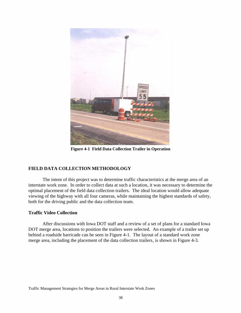
Figure 4-1 Field Data Collection Trailer in Operation
FIELD DATA COLLECTION METHODOLOGY
The intent of this project was to determine traffic characteristics at the merge area of aninterstate work zone. In order to collect data at such a location, it was necessary to determine theoptimal placement of the field data collection trailers. The ideal location would allow adequateviewing of the highway with all four cameras, while maintaining the highest standards of safety,both for the driving public and the data collection team.
Traffic Video Collection
After discussions with Iowa DOT staff and a review of a set of plans for a standard IowaDOT merge area, locations to position the trailers were selected. An example of a trailer set upbehind a roadside barricade can be seen in Figure 4-1. The layout of a standard work zonemerge area, including the placement of the data collection trailers, is shown in Figure 4-3.
Traffic Management Strategies for Merge Areas in Rural Interstate Work Zones
38

Figure 4-2 View of Electronic Equipment in a Data Collection Trailer
16 ft780 ft500 ft50 ft
Flashing Arrow Board
Data Collection Trailer Taper, w/ Drums every 65 ft Type III Barricade
Data Collection Trailer
Direction of Traffic
Direction of Traffic
Figure 4-3 Typical Location of Field Data Collection Trailers
Traffic Management Strategies for Merge Areas in Rural Interstate Work Zones
39

This layout provided increased safety for the project team by allowing the setup andoperation of the data collection trailers while staying behind existing equipment and barricades.These locations also made the trailers less conspicuous to motorists, as the trailers were at leastpartially shielded from view. This basic layout was used throughout the data collection phasewith little variation. Note that in Figure 4-3, the left lane is closed. In situations where the rightlane is closed the locations of the flashing arrow board, drums, barricade, and trailers would beplaced on the right-hand side of the highway rather than the left.
Once the equipment was in position, the traffic was recorded on videotape. One cameraon each trailer was positioned to record traffic just upstream from the trailer, with the secondcamera in each pair looking downstream. The layout described above allows the trailers tocollect video images of vehicles as they passed the flashing arrow board and as they passed theend of the taper in the transition area.
Once the trailers were in place and operating, a calibration grid was painted on theshoulders of the highway within the field of view of each camera. This grid was required to usethe Autoscope Supervisor software during the laboratory analysis to accurately determine thespeeds and lengths of the vehicles.
The marks for the grid were placed on the highway shoulders. Each mark was made withwhite paint and in the shape of rectangles measuring 8" by 16". The distances and anglesbetween each of the marks were accurately measured using a total station. This surveying toolallowed distance accuracy of 0.1 ft and angle accuracy of 10 seconds of one degree. The use ofthe total station allowed accurate measurements without requiring the personnel or theequipment to be in the traveled lanes. An example of a completed calibration grid is shown inFigure 4-4.
Queue Length Data Collection
When a queue developed, the project team would move to the outside shoulder of theinterstate, adjacent to the opposite direction of traffic. From this location, a project teammember in a vehicle followed the upstream end of the queue without causing additionaldisturbances to the queued traffic. The data collection team was able to safely follow and recordthe queue length over time, using the milepost markings on the reflectorized delineator posts inthe ditch to record the location of the end of the queue. This information was a necessarycomponent in determining an estimate of the number of vehicles in the queue, which was usedlater to determine the total delay cost of the observed queues. An example of this process can befound in Figure 4-5.
Traffic Management Strategies for Merge Areas in Rural Interstate Work Zones
40

Figure 4-4 Typical Placement of a Calibration Grid
Data Collection Vehicle. Moves with the upstreamend of the queue, records position over time.
End of queueTo Work Zone
Figure 4-5 Example of Collection of Queue-Length Data
RESULTS OF SUMMER DATA COLLECTION
Traffic backups were observed on Interstate 80 at Davenport on June 19, July 2, July 10,and August 7, 1998. Traffic volumes rose high enough that not all vehicles could be
Traffic Management Strategies for Merge Areas in Rural Interstate Work Zones
41

accommodated at their desired speed. Congestion and delays resulted, and were recorded by theproject team.
The other main site where data were collected was on Interstate 80 at the Rock RiverBridge in Illinois. However, no usable data were collected here, as traffic levels neverapproached capacity during the site visit. Other potential sites were not visited for variousreasons. The sites near Des Moines were excluded because the work was performed at night.The maintenance work that was performed on Interstate 380 between Cedar Rapids and IowaCity was switched to night work by the Iowa DOT to prevent congestion, which eliminated it asa usable site for our needs. The maintenance project on Interstate 35 north of Des Moines andthe maintenance project on Interstate 74 in urban Davenport did not start until after the end ofthe summer. Table 4-2 shows the dates and locations of the field data collection.
Table 4-2 Summary of Data Collection Dates and Locations
IM-80-8(171)295--13-82, Interstate 80 near Davenport8/21/98IM-80-8(171)295--13-82, Interstate 80 near Davenport8/14/98IM-80-8(171)295--13-82, Interstate 80 near Davenport8/7/98
Interstate 80 at the Rock River Bridge, Illinois7/31/98Interstate 80 at the Rock River Bridge, Illinois7/30/98Interstate 80 at the Rock River Bridge, Illinois7/29/98Interstate 80 at the Rock River Bridge, Illinois7/26/98
IM-80-8(171)295--13-82, Interstate 80 near Davenport7/17/98IM-80-8(171)295--13-82, Interstate 80 near Davenport7/10/98IM-80-8(171)295--13-82, Interstate 80 near Davenport7/9/98IM-80-8(171)295--13-82, Interstate 80 near Davenport7/3/98IM-80-8(171)295--13-82, Interstate 80 near Davenport7/2/98IM-80-8(171)295--13-82, Interstate 80 near Davenport7/1/98IM-80-8(171)295--13-82, Interstate 80 near Davenport6/30/98IM-80-8(171)295--13-82, Interstate 80 near Davenport6/26/98IM-80-8(171)295--13-82, Interstate 80 near Davenport6/19/98IM-80-8(171)295--13-82, Interstate 80 near Davenport5/29/98IM-80-8(171)295--13-82, Interstate 80 near Davenport5/28/98IM-80-8(171)295--13-82, Interstate 80 near Davenport5/27/98
Data Collection LocationDate
Limitations of Data Collection at the Davenport Location
The capacity of the merge areas was reached on only four occasions while the projectteam was on site. There are several possible reasons why more backups were not observed. Onereason is that the work zone was only four miles east of the Interstate 80/280 system interchange.Signs warning of several work zones on Interstate 80 were placed at the interchange,encouraging the use of Interstate 280 as an alternate route for eastbound traffic to bypass thework zones. This bypass possibly reduced volumes on Interstate 80 at the work zone enough toprevent some backups.
The work zone merge area for the westbound traffic was placed just downstream from anonramp with an acceleration lane adjacent to the traveled lanes. This resulted in giving theinterstate a three-lane configuration at the point of the merge. In order to minimize the
Traffic Management Strategies for Merge Areas in Rural Interstate Work Zones
42

variations in the geometry, the study was confined to the merge area for the eastbound traffic atthis work zone.
Figure 4-6 Location of the Data Collection Site at Davenport
SUMMARY
This methodology allowed the project team to collect video data of vehicles as theypassed the flashing arrow board and the end of the merge taper of an interstate work zone. Thesevideo images were analyzed using the Autoscope 2004 Machine Vision Processor to convert thevideo into vehicle characteristics, such as vehicle speed, length, and lane choice. This processwill be explained in Chapter 6.
Traffic Management Strategies for Merge Areas in Rural Interstate Work Zones
43

Traffic Management Strategies for Merge Areas in Rural Interstate Work Zones
44

CHAPTER 5 LABORATORY DATA REDUCTION
The SVHS tapes with traffic recordings were brought back to the laboratory and analyzedby the Autoscope 2004 Wide Area Vehicle Detection System. Traffic characteristics of eachvehicle were recorded and saved as text files using the Autoscope, and then imported intospreadsheet format for further analysis.
AUTOSCOPE DATA REDUCTION
The Autoscope detects changes in the visual images it receives to determine vehiclecharacteristics such as speed and length. It also is able to determine the characteristics of theentire traffic stream, such as the total number of vehicles that it detects in a given time period.The Autoscope uses a technology called machine vision processing to determine these trafficflow characteristics. A simple explanation of machine vision processing is that the Autoscopelooks for color changes in each pixel on the screen image. Determining when and how fast thesepixels change color is how the Autoscope determines a vehicle's characteristics and to theindividual vehicle characteristics are aggregated to derive traffic flow characteristics.
To receive accurate readings from the Autoscope, the system was calibrated using thecalibration feature in the Autoscope Supervisor software. Using the painted grid marksexplained in the previous chapter, an accurate calibration grid was drawn. The software requiresthat at least five virtual lines be placed over the top of the screen image in the shape of a grid.This grid is formed with lines running both parallel and perpendicular to the direction of trafficflow. The height of the camera above the highway is also required to complete the calibration.This provides the Autoscope with enough information to determine the plane in which traffic istraveling. An example of this setup is shown in Figure 5-1. With this, the Autoscope canobserve images on the videotape and determine the speed and length of each vehicle.
Using the Supervisor software, virtual detectors were placed over the image of the trafficlanes. These detectors were then used to determine each vehicle's speed, length, andclassification, much like loop detectors would if placed at that location. The proper placement ofthese detectors provides the lane distribution for the traffic at the flashing arrow board.Determining the lane distribution was not necessary for the video taken at the end of the mergearea because traffic had merged into one lane by that point. Figure 5-2 shows an example of twovirtual detectors placed over the highway near the flashing arrow board upstream from the mergearea.
Once the virtual detectors were designed for each camera view, the detector files weredownloaded into the Autoscope. With these files in place, the Autoscope could analyze thevideotapes and record the traffic characteristics. The Autoscope is capable of reading data fromtwo video feeds at one time. The data collected in this manner was then downloaded into thehard drive of the laboratory desktop computer for further analysis.
Traffic Management Strategies for Merge Areas in Rural Interstate Work Zones
45

Figure 5-1 Example of Autoscope Supervisor Calibration Grid
SUMMARY
The SVHS tapes were brought back to the laboratory, and the speed, length, and lanechoice for each vehicle were determined using the Autoscope 2004. The calibration grid paintedon the shoulders of the highway was used to calibrate the Autoscope software. This increasedthe accuracy of the data. Once the data reduction process was completed, the vehicular datawere downloaded from the Autoscope to a desktop computer for further analysis.
Traffic Management Strategies for Merge Areas in Rural Interstate Work Zones
46
Figure 5-2 Example of Virtual Detectors Placed over Video Image
Traffic Management Strategies for Merge Areas in Rural Interstate Work Zones
47

Traffic Management Strategies for Merge Areas in Rural Interstate Work Zones
48

CHAPTER 6: ANALYSIS AND RESULTS
This chapter details the analysis of the traffic data from the Davenport work zone. Theresults obtained include an improved estimate of the capacity of a standard Iowa DOT work zonemerge area, queue data including the lengths of the observed queues, how the upstream end ofthese queues behaved, and an estimate of the user cost incurred by motorists in these queues.This chapter ends with some recommendations about how this information can be used toimprove the planning process for future interstate work zones.
CAPACITY
Traffic backups were observed on Interstate 80 at Davenport on June 19, July 2, July 10,and August 7, 1998. Data for these dates were analyzed to determine how traffic operatedduring congestion.
Determining Capacity
The traffic flow data that were collected for the four days and the corresponding vehicleclassification percentages are shown in Tables 6-1 and 6-2 to illustrate the type and amount oftraffic observed. The units for Table 6-1 are in vehicles per hour.
Table 6-1 Observed Unconverted Traffic Volumes
52601,5294,6911,5814,7512 - 7 pm8/7/9824292,0068,3922,0308,4218 am- 6 pm7/10/98
2,0689,9983716382,43910,6369 am-9 pm7/2/981,4135,328811901,4945,5181-7 pm6/19/98
TrucksCarsTrucksCarsTrucksCarsRightLeft
By LaneTotalTimeDate
Table 6-2 Observed Unconverted Traffic Percentages
46.4%53.6%24.6%75.4%25.0%2-7 pm8/7/9845.2%54.7%19.3%80.7%19.4%8 am-6 pm7/10/9817.1%82.9%36.8%63.2%18.7%9 am-9 pm7/2/9821.0%79.0%29.9%70.1%21.3%1-7 pm6/19/98TrucksCarsTrucksCars
RightLeft
% By LaneTotal %Trucks
TimeDate
Traffic volumes are converted to passenger car equivalents from the observed datacollected with the field equipment. Trucks are converted to 1.5 passenger cars, which is takenfrom the 1994 Highway Capacity Manual for trucks on a level grade.(58) These converted datawere then analyzed in five-minute increments to determine the traffic volume in passenger carequivalents.
Traffic Management Strategies for Merge Areas in Rural Interstate Work Zones
49

The capacity of a work zone is really the highest volume observed immediately beforethe flow breaks down and queuing begins. Once queuing begins, the traffic volume passingthrough the work zone is really a measure of the queue discharge rate. Therefore, the highestvolumes immediately before a queue occurs are considered to be indicative of a work zone'scapacity and these values are measured. This measure of capacity was defined by Jiang. Jiangfound that the highest sustained free flow volumes through a work zone tend to occur just priorto a sharp speed drop.(59)
On July 2 and July 10, 1998, data were collected continuously from early morning untilevening. The data gathered during the time a queue was present were temporarily set aside inorder to examine only the free flow data. The ten highest converted free flow values wereidentified for each day. These data were studied to determine a pattern to the peak free flowvalues. As shown in Figure 6-1, when averaged over five-minute time increments, eight of theten highest free flow values on July 2 occurred within 1 hour and 45 minutes prior to thebeginning of the queue. On July 10, seven of the ten highest free flow values occurred within 90minutes of the breakdown and the beginning of the backup, as shown in Figure 6-2. Themajority of the highest free flow volumes occurred within two hours of the breakdowns on bothdays. The averages of the ten highest observed free flow values were calculated as anapproximation of the threshold volumes at which a breakdown could be expected.
The breakdowns on June 19 and August 7 were not analyzed in this manner because dataon these days were only collected for approximately two hours prior to queue development. Thisshorter range of time values did not allow for accurate comparisons of the highest free flowvalues against data for the entire day. These traffic flows just prior to the onset of the majorspeed drop and the beginning of queued conditions on these days were comparable to the July 2and July 10 data. The graphs of the traffic flows and speeds for June 19 and August 7 can befound in Figures 6-3 and 6-4.
Table 6-3 shows both the peak volume and the mean average for the ten highest free-flowvolumes for each day that a queue developed. The highest individual value of 1,746passenger-cars-per-hour (pcph) was observed, based on one five-minute period, on July 10.From the traffic observed, the mean value is in the range of 1,374 to 1,630 passenger cars perhour. The variation in volumes observed could be due to variations in the mix of vehicles,drivers, and driver interaction with other vehicles in the traffic stream. Note that convertingfrom vehicles per hour to passenger cars per hour raises the traffic flow values by 8 to 13percent.
Traffic Management Strategies for Merge Areas in Rural Interstate Work Zones
50

Flow and Speed Over Time7/2/98, I-80, Davenport, IA
Traffic at Merge Area
0
20
40
60
80
100
120
1408:
008:
158:
308:
459:
009:
159:
309:
4510
:00
10:1
510
:30
10:4
511
:00
11:1
511
:30
11:4
512
:00
12:1
512
:30
12:4
513
:00
13:1
513
:30
13:4
514
:00
14:1
514
:30
14:4
515
:00
15:1
515
:30
15:4
516
:00
16:1
516
:30
16:4
517
:00
17:1
517
:30
17:4
518
:00
18:1
518
:30
18:4
519
:00
19:1
519
:30
19:4
520
:00
20:1
520
:30
20:4
521
:00
21:1
521
:30
Time
Passenger Cars, Total (Pass. Cars/5 Min.) Average Speed, Total (mph)
Queued ConditionsFree Flow Conditions Free Flow Conditions
Ten Highest FreeFlow Values
Figure 6-1 Analysis of Ten Highest Converted Free Flow Values, 7/2/98
Flow and Speed Over Time7/10/98, I-80, Davenport, IA
Traffic at Merge Area
0
20
40
60
80
100
120
140
160
7:00
7:15
7:30
7:45
8:00
8:15
8:30
8:45
9:00
9:15
9:30
9:45
10:0
010
:15
10:3
010
:45
11:0
011
:15
11:3
011
:45
12:0
012
:15
12:3
012
:45
13:0
013
:15
13:3
013
:45
14:0
014
:15
14:3
014
:45
15:0
015
:15
15:3
015
:45
16:0
016
:15
16:3
016
:45
17:0
017
:15
17:3
017
:45
18:0
018
:15
18:3
018
:45
19:0
019
:15
Time
Passenger Cars, Total (Pass. Cars/5 min.) Average Speed, Total (mph)
QueuedConditions
Free Flow Conditions Free Flow Conditions
Ten Highest FreeFlow Values
Figure 6-2 Analysis of Ten Highest Converted Free Flow Values, 7/10/98
Traffic Management Strategies for Merge Areas in Rural Interstate Work Zones
51

Figure 6-3 Traffic Volumes and Speeds, 8/7/98
Figure 6-4 Traffic Volumes and Speeds, 6/19/98
Traffic Management Strategies for Merge Areas in Rural Interstate Work Zones
52
Flow and Speed Over Time6/19/98, I-80, Davenport, IA
Traffic at Merge Area
0
20
40
60
80
100
120
140
12:0
0
12:1
5
12:3
0
12:4
5
13:0
0
13:1
5
13:3
0
13:4
5
14:0
0
14:1
5
14:3
0
14:4
5
15:0
0
15:1
5
15:3
0
15:4
5
16:0
0
16:1
5
16:3
0
16:4
5
17:0
0
17:1
5
17:3
0
17:4
5
18:0
0
18:1
5
18:3
0
18:4
5
19:0
0
19:1
5
19:3
0
Time
Passenger Cars, Total (Pass. Cars/5 Min.) Average Speed, Total (mph)
Flow and Speed Over Time8/7/98, I-80, Davenport, IA
Traffic at Flashing Arrow Board
0
20
40
60
80
100
120
140
160
18013
:00
13:1
5
13:3
0
13:4
5
14:0
0
14:1
5
14:3
0
14:4
5
15:0
0
15:1
5
15:3
0
15:4
5
16:0
0
16:1
5
16:3
0
16:4
5
17:0
0
17:1
5
17:3
0
17:4
5
18:0
0
18:1
5
18:3
0
18:4
5
19:0
0
Time
Passenger Cars, Total (Pass. Cars/5 Min.) Average Speed, Total (mph)

Table 6-3 Observed Capacity Values During Free-Flow Conditions
1493175213751572Free Flow8/7/981630168014381524Free Flow7/10/981442154213021392Free Flow7/2/981374154212161284Free Flow6/19/98
Mean of 10HighestVolumes(pcph)
HighestVolume(pcph)
Mean of 10HighestVolumes(veh/hr)
HighestVolume(veh/hr)
Converted Free-Flow VolumesUnconverted Free-FlowVolumes
TrafficConditions
Date
QUEUE LENGTH
The length of the queues for these dates was monitored, with the length to the nearest0.05 miles recorded every minute. To accomplish this, the project team drove a vehicle on theopposite shoulder of the interstate in the direction of the westbound traffic. The team kept thevehicle even with the upstream end of the eastbound queue, and recorded the milepost readingsfrom the delineator posts in the ditch. The lengths of the queues over time are shown in Figures6-5 through 6-8.
The speeds of vehicles in the queue were determined from the videotapes of traffic as itpassed the cameras stationed behind the flashing arrow board. The average speed of vehiclesthat passed the data collection equipment during queued conditions was determined. This wasdone for each lane of traffic, and was used as an approximation of the speed of traffic over theentire queue. This process was repeated for each day. The average headway for each lane oftraffic was also determined. The calculated average speeds and headways, by lane, can be foundin Table 6-4. Dividing the observed queue length by the average headway in each lane providedan estimate of the total number of vehicles in each lane of the queue. Taking the average speedand the length of the queue, it was determined that the longest delay for any vehicle was aboutfive minutes. It should be noted that the closed lane on June 19 and July 2 was the left lane, andthe closed lane on July 10 and August 7 was the right lane. In each case, fewer vehicles madeuse of the closed lanes, resulting in larger headways.
Table 6-4 Observed Traffic Characteristics under Queued Conditions
29.621.038558621.621.22.78 hours8/7/9844.415.041858625.322.60.97 hours7/10/9812.819.56947216.818.13.70 hours7/2/9813.131.767143116.917.73.68 hours6/19/98
RightLane
LeftLane
RightLane
LeftLane
RightLane
LeftLane
Percent Trucks (%)Average Headway(ft)
Average Speed(mph)Queue
DurationDate
Figure 6-5 Queue Length on 6/19/98
Traffic Management Strategies for Merge Areas in Rural Interstate Work Zones
53

Figure 6-6 Queue Length on 7/2/98
Traffic Management Strategies for Merge Areas in Rural Interstate Work Zones
54
0
0.2
0.4
0.6
0.8
1
1.2
1.4
1.6
1.8
3:10
PM
3:21
PM
3:32
PM
3:43
PM
3:54
PM
4:05
PM
4:16
PM
4:27
PM
4:38
PM
4:49
PM
5:00
PM
5:11
PM
5:22
PM
5:33
PM
5:44
PM
5:55
PM
6:06
PM
6:17
PM
6:28
PM
6:39
PM
6:50
PM
7:01
PM
Time
Que
ue L
engt
h (m
iles)
Length of Queue
0
0.2
0.4
0.6
0.8
1
1.2
1.4
1.6
3:00
PM
3:10
PM
3:20
PM
3:30
PM
3:40
PM
3:50
PM
4:00
PM
4:10
PM
4:20
PM
4:30
PM
4:40
PM
4:50
PM
5:00
PM
5:10
PM
5:20
PM
5:30
PM
5:40
PM
5:50
PM
6:00
PM
6:10
PM
6:20
PM
6:30
PM
6:40
PM
Time
Que
ue L
engt
h (m
iles)
Length of Queue
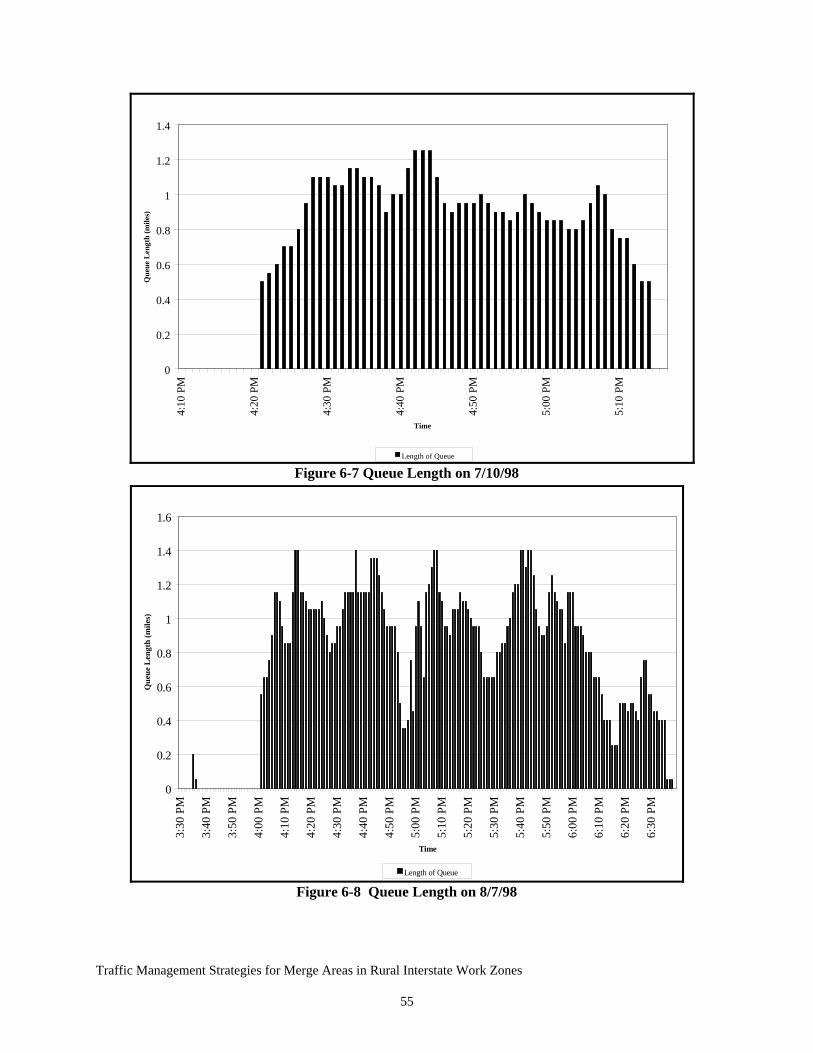
Figure 6-7 Queue Length on 7/10/98
Figure 6-8 Queue Length on 8/7/98
Traffic Management Strategies for Merge Areas in Rural Interstate Work Zones
55
0
0.2
0.4
0.6
0.8
1
1.2
1.4
4:10
PM
4:20
PM
4:30
PM
4:40
PM
4:50
PM
5:00
PM
5:10
PM
Time
Que
ue L
engt
h (m
iles)
Length of Queue
0
0.2
0.4
0.6
0.8
1
1.2
1.4
1.6
3:30
PM
3:40
PM
3:50
PM
4:00
PM
4:10
PM
4:20
PM
4:30
PM
4:40
PM
4:50
PM
5:00
PM
5:10
PM
5:20
PM
5:30
PM
5:40
PM
5:50
PM
6:00
PM
6:10
PM
6:20
PM
6:30
PM
Time
Que
ue L
engt
h (m
iles)
Length of Queue

The American Association of State Highway and Transportation Official's (AASHTO)"Manual on User Benefit Analysis of Highway and Bus-Transit Improvements," shows that thevalue of time savings for automobiles is not a constant value per minute over all time ranges.Three ranges of time saving values were established from zero to five minutes, five to tenminutes, and over ten minutes. For delay times from zero to five minutes, the delay value isconsidered only 50 percent of the value assigned for longer time periods.(60) As the longestdelays observed were about five minutes, 50 percent of the hourly rate will be used below whendetermining the delay cost for passenger cars.
Values for delay were taken from the Iowa DOT's Guide to the Economic Evaluation ofHighway Projects, hereafter referred to as the Guide.(61) The Guide provides an average wagerate of $11.65 per hour. This value was then converted from 1992 dollars to 1998 dollars using aconversion of 1.1611, the change in the Consumer Price Index during that time.(62) Thecalculations for the delay costs for passenger cars were made in the same manner as in theGuide, assuming that there were 1.87 people per passenger car, and that non-business trips arevalued at 40 percent of the rate for business trips. Business trips were estimated at one-third ofall passenger car trips, with non-business trips estimated as the remaining two-thirds ofpassenger car trips. The ratio is slightly different from the 0.3 and 0.7 values found in the Guide.The calculation for the passenger car delay time was calculated as follows:
Portion of hourly cost due to business travelers = [$11.65 * 1.1611 * 1.87 * 1/3] = $8.43
Portion of hourly cost due to non-business travelers =[$11.65 * 0.4 * 1.1611 * 1.87 * 2/3] = $6.74
Total hourly delay cost for passenger cars = $8.43 + $6.74 = $15.17
Total hourly cost for passenger cars with 0 to 5 minutes delay = $15.17 * 0.5 = $7.58
This allows the use of a single value for the value of automobile travel time of $7.58 perhour.
The Guide provides a delay cost of $16.25 for single-unit and tractor-trailer trucks. Bymultiplying $16.25 by 1.1611 to bring it to 1998 dollars, the rate of $18.87 per hour was found.This value was used for the calculation of truck delay costs.
The estimated costs of delay were calculated for each minute of the observed queue, andthese were summed to provide data for the total delay cost for each queue. The results areprovided in Table 6-5. Data were also divided by the time each queue was present in order tofind the hourly cost estimate for each queue.
Due to the lack of queue density information available for vehicles upstream of theflashing arrow board, more accurate delay calculations cannot be made. It is likely that a higherconcentration of vehicles may have used the closed lane upstream of the flashing arrow board,but without quantifiable data, this cannot be verified. This would tend to indicate that thesedelay costs are conservative.
Traffic Management Strategies for Merge Areas in Rural Interstate Work Zones
56

Table 6-5 Economic User Delay Costs for Observed Queues
$529.94$1,4752.78 hours8/7/98$498.62$4820.97 hours7/10/98$682.16$2,5243.7 hours7/2/98$616.29$2,2703.68 hours6/19/98
Cost Per HourEconomic User DelayCost
Queue DurationDate
Behavior of the Upstream End of the Queues
The position of the upstream end of the observed queues was recorded over time todetermine the overall length of the queue. Several graphs were prepared showing the speed atwhich the upstream end of the queues changed position. As can be seen in Figures 6-5 through6-8, the location of the end of the queue was very unstable, and could quickly move to a newlocation. These figures were prepared using the position information that was recorded in thefield. The speeds were determined by dividing the distance the end of the queue moved by oneminute. When the end of the queue was moving upstream, the total queue was growing longer,due to more vehicles entering the queue than could be accommodated at the merge point. Trafficapproaching the end of the queue while the queue was lengthening could be unprepared to stop,not realizing that the end of the queue was actually moving toward them. From Figures 6-9through 6-12 it can be seen that the end of the queue moved upstream from five to ten miles perhour over short time periods, and at times the queue moved at speeds as high as 30 miles perhour.
This change in direction and speed of the end of the queues often caused many dangerousdriving situations for motorists. Every observed queue had instances of motorists requiring hardbraking or quick lane changes to avoid rear-ending the vehicles at the end of the queue. Whileno crashes were observed, these numerous near misses clearly showed how a crash could easilyoccur due to work zone congestion.
Traffic Management Strategies for Merge Areas in Rural Interstate Work Zones
57

Figure 6-9 Speed Change of End of Queue, 6/19/98
Figure 6-10 Speed Change of End of Queue, 7/02/98
Traffic Management Strategies for Merge Areas in Rural Interstate Work Zones
58
-20
-15
-10
-5
0
5
10
15
3:10
PM
3:20
PM
3:30
PM
3:40
PM
3:50
PM
4:00
PM
4:10
PM
4:20
PM
4:30
PM
4:40
PM
4:50
PM
5:00
PM
5:10
PM
5:20
PM
5:30
PM
5:40
PM
5:50
PM
6:00
PM
6:10
PM
6:20
PM
6:30
PM
6:40
PM
6:50
PM
7:00
PM
Tim e
Spe
ed C
hang
e (m
ph)
Speed at End of Queue
-20
-15
-10
-5
0
5
10
15
3:10
PM
3:20
PM
3:30
PM
3:40
PM
3:50
PM
4:00
PM
4:10
PM
4:20
PM
4:30
PM
4:40
PM
4:50
PM
5:00
PM
5:10
PM
5:20
PM
5:30
PM
5:40
PM
5:50
PM
6:00
PM
6:10
PM
6:20
PM
6:30
PM
6:40
PM
6:50
PM
7:00
PM
Tim e
Spe
ed C
hang
e (m
ph)
Speed at End of Queue

Figure 6-11 Speed Change of End of Queue, 7/10/98
Figure 6-12 Speed Change of End of Queue, 8/7/98
Traffic Management Strategies for Merge Areas in Rural Interstate Work Zones
59
-40
-30
-20
-10
0
10
20
30
40
4:10
PM
4:15
PM
4:20
PM
4:25
PM
4:30
PM
4:35
PM
4:40
PM
4:45
PM
4:50
PM
4:55
PM
5:00
PM
5:05
PM
5:10
PM
5:15
PM
Tim e
Spe
ed C
hang
e (m
ph)
Speed at End of Queue
-30
-20
-10
0
10
20
30
40
3:30
PM
3:40
PM
3:50
PM
4:00
PM
4:10
PM
4:20
PM
4:30
PM
4:40
PM
4:50
PM
5:00
PM
5:10
PM
5:20
PM
5:30
PM
5:40
PM
5:50
PM
6:00
PM
6:10
PM
6:20
PM
6:30
PM
Tim e
Spe
ed C
hang
e (m
ph)
Speed at End of Queue

Traffic Management Strategies for Merge Areas in Rural Interstate Work Zones
60

CHAPTER 7 CONCLUSIONS AND RECOMMENDATIONS
Two significant findings are drawn from this research. First, a more valid valueof the capacity of an Iowa interstate work zone has been determined. One example ofhow this information could be used by the Iowa DOT to improve work zone traffic flowis shown in this chapter. Second, a quantifiable value of the cost imposed on motorists inwork zone-related queues at one work zone location has been established, and was shownin the previous chapter. This relatively low delay cost indicates that diversion to relievecongestion at an interstate work zone is not warranted where congestion-based delays areeither infrequent or where maximum delays are relatively short (ten minutes). A moreserious issue is the speed with which shock waves may move backwards. The upstreamgrowth of shock waves violates the expectation of drivers traveling at freeway speeds andhelps to result in unsafe conditions. Given that congestion on rural interstate highways isan inevitable externality of reconstruction and maintenance, highway agencies, like theIowa DOT, should concentrate on alerting drivers of approaching queues. Further, webelieve that informing drivers of the length of delays they can reasonably expect can helpto reduce driver aggressiveness (“road rage”).
WORK ZONE CAPACITY
Based on the data collected at one work zone on Interstate 80 near Davenport,traffic capacity at Iowa's work zone merge areas was found to be from 1,374 to 1,630passenger cars equivalents per hour when two lanes were reduced to one. One use forthis information would be to determine which upcoming work zones would potentiallyrequire additional traffic control. Simply examining the previous year's traffic datacollected at Automatic Traffic Recorder locations near the planned location of anupcoming work zone could provide insight as to when traffic congestion might occur.For example, Figure 7-1 provides average westbound traffic flow data from the ATR#111, near Williamsburg on Interstate 80.(63) These data were taken from the month ofJuly 1997, and averaged by day of the week. As shown in the Figure 7-1, Friday andSunday afternoons tended, on average, to have enough traffic flow to potentially createcongestion based on the capacity levels observed in Davenport. This would indicate thata work zone placed here in future years could expect queues on Friday and Sundayafternoons in July if no additional traffic management efforts are planned. By analyzingtraffic levels at future work zone locations in this manner, the DOT could target anenhanced traffic management program to the times when it would be most needed,thereby providing the most effective use of limited resources.
The value of 1,216 vehicles per hour used as the threshold of work zonecongestion in Figure 7-1 is taken from Table 6-3, and is the lowest mean capacity valueobserved at the Davenport location. If this figure had been prepared in passenger carequivalent units, a low value of 1,374 would have been used, again taken from Table 6-3.
Traffic Management Strategies for Merge Areas in Rural Interstate Work Zones
61

Average Daily Traffic Flows by Day of WeekATR #111, I-80 Near Williamsburg, IA, July 1997
0
200
400
600
800
1000
1200
1400
1600
1 2 3 4 5 6 7 8 9 10 11 12 13 14 15 16 17 18 19 20 21 22 23 24
Hour of the Day
Traf
fic F
low
s (V
eh/H
r)
Sunday Monday Tuesday Wednesday Thursday Friday Saturday
1,216 Veh/Hr. Threshold of Work Zone Congestion
Figure 7-1 Using Capacity Values to Determine if Congestion Might Occur
WORK ZONE DELAY COST IMPOSED ON MOTORISTS
This study also found that the four observed queues cost a total of approximately$6,751.00 in economic delay to motorists, as shown in Chapter 6. Hourly delay cost ratesfor the observed queues range from $589.62 to $682.16, with an average value of$606.38 per hour of congestion.
The delays observed at the Davenport location were, in general, never more thanabout five minutes. For such short delay times, one effective solution could be to applythe Ohio devices which estimate the time required to reach the merge area and posts theestimate to a changeable message sign. This would provide motorists with informationneeded to realize that the delay is a short one, and should serve to reduce driverfrustration. No other possible improvements seem cost-effective due to the low delaycost and the few times that congestion-based queues were observed.
No crashes were associated with the observed queues, but several near misseswere observed as motorists were forced to break to avoid the upstream end of the queue.Any one of these near misses could have resulted in a crash, significantly increasing thecost to the public, crash costs and additional delays for other motorists. Determining anestimate of the number of crashes that result due to work zone congestion would providean even better picture of the benefit motorists would realize due to improved traffic
Traffic Management Strategies for Merge Areas in Rural Interstate Work Zones
62

management. A crash analysis was beyond the scope of this study, and no crashes wereobserved while the data collection equipment was in place.
Traffic Management Strategies for Merge Areas in Rural Interstate Work Zones
63

17. Dixon, K.K., Hummer, J.E., and Rouphail, N.M., “Comparison of Rural Freeway Work
16. Persaud, B., Yager, S., and Brownlee, R., “Exploration of the Breakdown Phenomenon inFreeway Traffic,” Transportation Research Board Annual Meeting, Washington, D.C.,January, 1998.
15. Hall, F.L. and Agyemang-Duah, K., “Freeway Capacity Drop and Definition ofCapacity,” Transportation Research Record 1320, National Research Council,Washington D.C., 1991.
14. Zhou, M., and Hall, F.L., “Investigation of the Speed-Flow Relationship UnderCongested Conditions on a Freeway,” Presented at the Transportation Research BoardAnnual Meeting, Washington, D.C., January, 1999.
13. Ringer, J. and Urbanik, T., “Study of Freeway Bottlenecks in Texas,” TransportationResearch Records 1398, National Research Council, Washington, D.C., pp. 31 - 41,1993.
12. Wemple, E.A., Morris. A.M., and May, A.D., “Freeway Capacity and Level of ServiceConcepts,” Highway Capacity and Level of Service, Proceedings of the InternationalSymposium on Highway Capacity, Karlsruhe, Rotterdam: Balkema, pp. 439 - 455.
11. Chin, H.C. and May, A.D., “Examination of the Speed-Flow Relationship at theCaldecott Tunnel,” Transportation Research Record 1320, National Research Council,Washington, D.C., 1991.
10. Hall, F.L., and Hall, L.M., “Capacity and Speed Flow Analysis of the Queue in Ontario,”Transportation Research Record 1287, National Research Council, Washington, D.C., pp.108 - 118, 1990.
9. Banks, J.H., “Flow Processes at a Freeway Bottleneck,” Transportation Research Record1287, National Research Council, Washington, D.C., pp.83 - 90, 1320.
8. Banks, J.H., “Freeway Speed-Flow Concentration Relationships: More Evidence andInterpretations,” Transportation Research Record 1225, National Research Council,Washington, D.C., pp. 53 - 60, 1989.
7. Hall, F.L., Hurdle, V.F., and Banks, J.H., “Synthesis of Recent Work on the Nature ofSpeed-Flow and Flow-Occupancy (Or Density) Relationships on Freeways,”Transportation Research Board Record 1365, National Research Council, Washington,D.C., pp. 12 -18.
6. Gurlough, D.L., and Huber, M.J., “Traffic Flow Theory: A Monograph,” TransportationResearch Board Special Report 165, Washington, D.C., 1975, p. 51.
5. Drake, J.S., Schofer, J., and May, A.D., “A Statistical Analysis of Speed-DensityHypothesis,” Proceedings of the Third International Symposium on Theory of TrafficFlow, New York, NY, June, 1965, pp. 112 - 117.
4. Underwood, R.T., “Speed, Volume, and Density Relationships,” Quality and Theory ofTraffic Flow, Bureau of Highway Traffic, Yale University, New Haven, CT, 1961, pp141 - 187.
3. Greenberg, H., “An Analysis of Traffic Flow,” Operations Research, Vol. 7, No. 1, pp.79 - 85, 1959.
2. Greenshields, B.D., “A Study of Traffic Capacity, Highway Research Board Proceedings,Vol. 14, Washington, D.C., 1934, pp.448 - 477.
1. “Highway Capacity Manual,” Transportation Research Board Special Report 209,Washington, D.C., 1994, p. A-4.

33. Byrd, P.S., Geza, P., Jessen, D.S., and McCoy, P.T., “Driver Survey of the Late-MergeWork Zone Traffic Control Strategy,” Presented to the 78th Annual Meeting of theTransportation Research Board, Washington, D.C., 1999
32. Rouphail, N.M. and Nemeth, Z.A., “Human Factors Considerations as FreewayConstruction Lane Closures,” ITE Journal, Vol. 52, 1982, pp. 37-44.
31. Dudek, C.L. and Richards, S.H., “Traffic Management for Middle Lane Maintenance onUrban Freeways,” Prepared by the Texas Transportation Institute, Prepared for theFederal Highway Administration and the Texas Department of Transportation, Austin,TX, Report No. FHWA/TX-80/3+228-1, 1980.
30. Richards, S.H., and Dudek, C.L., “Field Evaluation of Traffic Management Strategies forMaintenance Operations in Freeway Middle Lanes,” Transportation Research Record703, 1979, pp. 31-36.
29. Kermode, R.H., and Myra, W.A., “Freeway Lane Closures,” Traffic Engineering Vol. 40,No. 5, 1970, pp. 14-18.
28. Dudek, C.L. and Richards, S.H., “Traffic Capacity Through Urban Freeway Work Zonesin Texas,” Transportation Research Record 869, 1982, pp. 14-18.
27. Krammes, R.A., and Lopex, G.O. “Updated Short-Term Freeway Work Zone LaneClosures Capacity Values,” Prepared by the Texas Transportation Institute, Prepared forthe Federal Highway Administration and the Texas Department of Transportation,Austin, TX, Report No. FHWA/TX-92-/1108-5, 1992.
26. Byington, S., “Frequency and Location of Rear-End and Side-swipe Work ZoneAccidents,” Federal Highway Administration, McLean, VA, 1998. (Internal report)
25. Khattak, A.J., Khattak, A.J., and Council, F.M., “Analysis of Injury and Non-injuryCrashes in California Work Zones,” Presented at the Transportation Research BoardAnnual Meeting in Washington, D.C., 1999.
24. Pal, R. and Sinha, K.C., “Analysis of Crash Rates at Interstate Work Zones in Indiana,”Transportation Research Record 1529, 1995, pp. 43-53.
23. McShane, W.R. and Roess R.P., Traffic Engineering, New Jersey: Prentice-Hall, Inc.
22. Lighhill, M.J. and Whitham, G.B., “On Kinematic Waves: Part II, A Theory on LongCrowded Roads,” Proceedings of the Royal Society, Series A, 229 (1178), pp. 317-345,1955.
21. Memmott, J.L., and Dudek, C.L., “A Model to Calculate the Road User Cost at WorkZones,” Prepared by the Texas Transportation Institute, Prepared for the FederalHighway Administration and the Texas Department of Transportation, Austin, TX,Report No. FHWA/TX-83/20+292-1, 1982.
20. Dixon, K.K., and Hummer, J.E., “Capacity and Delay in Major Freeway Construction,”Prepared for the North Carolina Department of Transportation by the Center forTransportation Engineering Studies, North Carolina State University, Report No.23241-94-8, 1995.
19. Persaud, B. and Dzbik, L., “Accident Prediction Models for Freeways,” TransportationResearch Record 1401, pp. 55-60, 1993.
18. Jiang, Y., “Traffic Capacity, Speed, and Queue-Discharge Rate of Indiana’s Four-LaneFreeway Work Zones,” Presented at the Annual Meeting of the Transportation ResearchBoard, Washington, D.C., 1999.
Zones Queue Length Estimation Techniques: A Case Study,” Presented to TransportationResearch Board Annual Meeting, Washington, D.C., 1998.

50. Byrd, P.S., Pesti, G., Jessen, D.S. and McCoy, P.T., “Driver Survey of the Late-MergeWork Zone Traffic Control Strategy,” Presented to the Transportation Research Board78th Annual Meeting, Washington, D.C., 1999.
49. Shapiro, M.S., Pavis, A., Stafford, O.V., and Yogoda, J.H., “Applying ITS Technologyfor Safer Highway Construction Management,” Proceedings of the 68th Meeting of theInstitute of Transportation Engineers, Toronto, Ontario, Canada, 1998.
48. Pavis, A., Wilder, W.H., and Hunt, J.F., “Deployment of Rapid Deployment ITSElements to Support Construction Management,” Proceedings of the 68th Meeting of theInstitute of Transportation Engineers, Toronto, Ontario, Canada, 1998.
47. Private correspondence with Scientex Corporation regarding the ADAPTIRTM, 1997.
46. Boyd, S.J., “A Public - Private Partnership: Minnesota Smart Workzone Case Study,”Proceedings of the Annual ITS America Meeting, Washington, D.C., 1999.
45. Nookala, M., Dillingham, J.W., Melby, G., and Differt, D., “Smart Work Zone: ITSOperational Test Results,” Proceedings of the Annual ITS America Meeting, Detroit, MI,1998.
44. Churchill, B., and Cather, R., and Murphy, D., “San Diego’s Prototype IntermodalTransportation Management Center: A Southern California Priority Corridor ShowcaseProject,” Proceedings of the Annual ITS America Meeting, Detroit, MI, 1998.
43. “Commercial Vehicle Fleet Management and Information Systems, Phase 1, InterimReport,” Prepared by Cambridge Systematics, Inc., ATA Foundation, and the PrivateFleet Management Institute, Prepared for the Federal Highway Administration, ReportNo. DTFH61-93-C-00084, October, 1997, pp. 19 - 20.
42. Wright, B, Kaliski, J.G., and Pritchard, R.D., “Advanced Traveler Information Servicesfor Commercial Vehicle Operators: TruckDesk,” Proceedings of the Annual ITS AmericaMeeting, Washington, D.C., 1997.
41. Neudorff, L.G., Galley, D., and Wintermute, J., “The I-95 Corridor Coalition InformationExchange Network,” Proceedings of the Annual ITS American Meeting, Washington,D.C., 1997.
40. Pant, P.D., “Travel Time Predictions System (TIPS) for Freeway Work Zones,” Preparedfor the Ohio Department of Transportation by the University of Cincinnati, 1998.
39. Gent, S.J., “Rural Smart Work Zone: A Warning System for Motorists During InterstateReconstruction Projects,” Proceedings of the 68th Meeting of the Institute ofTransportation Engineers, Toronto, Ontario, Canada, 1998.
38. “Des Moines Metropolitan Area ITS Strategic Plan,” Prepared by the Center forTransportation Research and Education, Prepared for the Des Moines Area MPO, DesMoines, IA, 1997.
37. Herstein, H.I., Walczak, W., and Guerra, T.G., “Intelligent Management of RoadwayClosures and Restrictions,” Proceedings of the 67th Annual Meeting of the Institute ofTransportation Engineers, Boston, MA, 1997.
36. Jiang, Y, “A Model for Estimating Excess User Cost at Highway Workzone,” Presentedto the Transportation Research Board at its annual meeting, Washington, D.C., 1999.
35. Jiang, Y, “Dynamic Predication of Traffic Flow and Congestion at Freeway WorkZones,” Presented to the Transportation Research Board at its annual meeting,Washington, D.C., 1999
34. Rouphail, N.M. and Tiwari, G., “Flow Characteristics at Freeway lane Closures,”Transportation Research Record, 1035, 1985, pp. 50-58.

63. Monthly Summary of Traffic Recorder Data, Recorder No. 11130, Station No. 111, July1997, Provided by the Iowa Department of Transportation, Office of Transportation Data,Ames, IA.
62. Bureau of Labor Statistics Homepage, http://146.142.4.24/cgi-bin/surveymost February4, 1999.
61. “Guide to the Economic Evaluation of Highway Projects,” Prepared for the IowaDepartment of Transportation, Wilbur Smith Associates, 1993.
60. A Manual on User Benefit Analysis of Highway and Bus-Transit Improvements, American Association of State Highway and Transportation Officials, Washington D.C.,1977.
59. Jiang, Y., Traffic Capacity, Speed, and Queue-Discharge Rate of Indiana's Four-LaneFreeway Work Zones, Presented at the 78th Annual Transportation Research BoardMeeting, Washington, D.C., 1999.
58. Special Report 209, Highway Capacity Manual, Third Edition, Transportation ResearchBoard, National Research Council, Washington D.C., 1994.
57. Solarcorp, Movite Journal, Missouri Valley Section, Institute of TransportationEngineers, December, 1991, p. 4.
56. Turochy, R.E., and Sivanandan, R., “Effectiveness of Unmanned Radar as a SpeedControl Technique in Freeway Work Zones,” Presented to the Transportation ResearchBoard 77th Annual Meeting, Washington, D.C., 1998.
55. Ullman, G.L., and Riesland, D.R., “Catalog of Work Zone Speed Control Methods,”prepared for the Texas Department of Transportation by the Texas TransportationInstitute, College Station, TX, Report No. FHWA/TX-90/1161-2, 1990.
54. Pigman, J.G., Agent, K.R., Deacon, J.A., and Kryscio, R.J., “Evaluation of UnmannedRadar installations,” Transportation Research Record 1244, National Research Council,1989, pp. 7 - 16.
53. Tarko, A.P., Kanipakapatnam, R.K., and Wasson, J.S., “Modeling and Optimization ofthe Indiana Lane Merge Control System on Approaches to Freeway Work Zones,”Prepared for the Joint Transportation Research Program, Prepared by the PurdueUniversity, West Lafayette, IN, 1998.
52. Telephone discussion with Andrzeu Tarko, Assistant Professor of Civil Engineering,Purdue University, April, 1999.
51. “Freeway Construction Work Zone Safety Enhancement Report,” Prepared for thePennsylvania Department of Transportation, Prepared by Orth-Rodger and Associates,Inc., Philadelphia, PA, 1995.