WP/16/27

Trading on Their Terms? Commodity Exporters in the Aftermath of the Commodity

Boom

by Aqib Aslam, Samya Beidas-Strom, Rudolfs Bems, Oya Celasun, Sinem Kılıç Çelik, and Zsóka Kóczán

© 2016 International Monetary Fund WP/16/27

IMF Working Paper

Research Department

Trading on Their Terms? Commodity Exporters in the Aftermath of the Commodity

Boom1

Prepared by Aqib Aslam, Samya Beidas-Strom, Rudolfs Bems, Oya Celasun, Sinem

Kılıç Çelik, and Zsóka Kóczán

Authorized for distribution by Oya Celasun

February 2016

Abstract

Commodity prices have declined sharply over the past three years, and output growth has

slowed considerably among countries that are net exporters of commodities. A critical

question for policy makers in these economies is whether commodity windfalls influence

potential output. Our analysis suggests that both actual and potential output move together

with commodity terms of trade, but that actual output comoves twice as strongly as

potential output. The weak commodity price outlook is estimated to subtract 1 to 2¼

percentage points from actual output growth annually on average during 2015-17. The

forecast drag on potential output is about one-third of that for actual output.

JEL Classification: O13, P48, Q02, Q33

Keywords: Natural Resources , Potential Output, Resource Boom, Terms of Trade

Authors’ E-Mail Addresses: aaslam@imf.org; sbeidasstrom@imf.org; rbems@imf.org;

ocelasun@imf.org; skiliccelik@imf.org; zkoczan@imf.org

1 This paper is based on Chapter II of the IMF’s October 2015 World Economic Outlook. The authors thank

Olivier Blanchard, José de Gregorio, Thomas Helbling, Ben Hunt, Gian Maria Milesi-Ferretti, Maury Obstfeld,

Jorge Roldos, and participants at an IMF seminar for helpful suggestions and comments, Hao Jiang and

Christina Liu for excellent research assistance, Bertrand Gruss for providing the commodity terms of trade data,

and André Hofman for sharing the KLEMS dataset for Chile.

IMF Working Papers describe research in progress by the author(s) and are published to

elicit comments and to encourage debate. The views expressed in IMF Working Papers are

those of the author(s) and do not necessarily represent the views of the IMF, its Executive Board,

or IMF management.

3

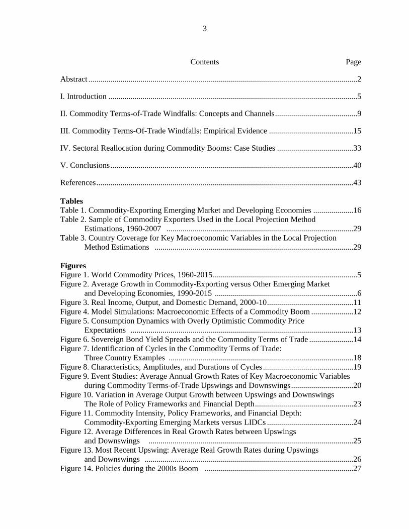
Contents Page

Abstract ......................................................................................................................................2

I. Introduction ............................................................................................................................5

II. Commodity Terms-of-Trade Windfalls: Concepts and Channels .........................................9

III. Commodity Terms-Of-Trade Windfalls: Empirical Evidence ..........................................15

IV. Sectoral Reallocation during Commodity Booms: Case Studies ......................................33

V. Conclusions .........................................................................................................................40

References ................................................................................................................................43

Tables

Table 1. Commodity-Exporting Emerging Market and Developing Economies ....................16

Table 2. Sample of Commodity Exporters Used in the Local Projection Method

Estimations, 1960-2007 .............................................................................................29

Table 3. Country Coverage for Key Macroeconomic Variables in the Local Projection

Method Estimations ...................................................................................................29

Figures

Figure 1. World Commodity Prices, 1960-2015 ........................................................................5

Figure 2. Average Growth in Commodity-Exporting versus Other Emerging Market

and Developing Economies, 1990-2015 .......................................................................6

Figure 3. Real Income, Output, and Domestic Demand, 2000-10 ...........................................11

Figure 4. Model Simulations: Macroeconomic Effects of a Commodity Boom .....................12

Figure 5. Consumption Dynamics with Overly Optimistic Commodity Price

Expectations ...............................................................................................................13

Figure 6. Sovereign Bond Yield Spreads and the Commodity Terms of Trade ......................14

Figure 7. Identification of Cycles in the Commodity Terms of Trade:

Three Country Examples ............................................................................................18

Figure 8. Characteristics, Amplitudes, and Durations of Cycles .............................................19

Figure 9. Event Studies: Average Annual Growth Rates of Key Macroeconomic Variables

during Commodity Terms-of-Trade Upswings and Downswings ...............................20

Figure 10. Variation in Average Output Growth between Upswings and Downswings

The Role of Policy Frameworks and Financial Depth .................................................23

Figure 11. Commodity Intensity, Policy Frameworks, and Financial Depth:

Commodity-Exporting Emerging Markets versus LIDCs ...........................................24

Figure 12. Average Differences in Real Growth Rates between Upswings

and Downswings ......................................................................................................25

Figure 13. Most Recent Upswing: Average Real Growth Rates during Upswings

and Downswings ........................................................................................................26

Figure 14. Policies during the 2000s Boom ..........................................................................27

4

Figure 15. Macroeconomic Variables in the Aftermath of Commodity

Terms-of-Trade Shocks .............................................................................................30

Figure 16. Output in the Aftermath of Commodity Terms-of-Trade Shocks:

Role of Income Level and Type of Commodity ........................................................31

Figure 17. Sectoral Composition of Output ..........................................................................34

Figure 18. Commodity Booms and Macroeconomic Indicators

in Australia, Canada, and Chile ..........................................................................35

Figure 19. Growth of Capital and Labor by Sector: Boom versus Preboom Periods ..............36

Figure 20. Evolution of Activity in Nontradables Relative to Manufacturing, Commodity

Exporters Relative to Commodity Importers ...........................................................39

5

I. INTRODUCTION

After rising dramatically for almost a decade, the prices of many commodities,

especially those of energy and metals, have dropped sharply since 2011 (Figure 1). Many

analysts have attributed the upswing in commodity prices to sustained strong growth in

emerging market economies, in

particular those in east Asia, and the

downswing to softening growth in

these economies and a greater supply

of commodities.2 Commodity prices

are notoriously difficult to predict, but

analysts generally agree that they will

likely remain low, given ample

supplies and weak prospects for global

economic growth. Commodity futures

prices also suggest that, depending on

the commodity, future spot prices will

remain low or rebound only moderately

over the next five years.

The decline in commodity

prices has been accompanied by stark

slowdowns in economic growth among

commodity-exporting emerging

market and developing economies,

most of which had experienced high

growth during the commodity price

boom (Figure 2). Besides the decline

in growth, commodity exporters have

seen downgrades in their medium-term

growth prospects: almost 1 percentage

point has been shaved off the average

of their five-year-ahead growth

forecasts since 2012, while the

2 The role of global and emerging market demand in driving the surge in commodity prices in the first decade of

the 2000s is discussed in Erten and Ocampo 2012, Kilian 2009, and Chapter 3 of the October 2008 World

Economic Outlook. On the impact of slowing emerging market growth on commodity prices, see “Special

Feature: Commodity Market Review” in Chapter 1 of the October 2013 World Economic Outlook. Roache 2012

documents the increase in China’s share in global commodity imports in the 2000s and Box 1.2 of the April

2014 World Economic Outlook examines the impact of China’s rebalancing on commodity consumption.

0

50

100

150

200

250

1960 65 70 75 80 85 90 95 2000 05 10 15

Figure 1. World Commodity Prices, 1960–2015(In real terms; index, 2005 = 100)

1. Energy and Metals

Sources: Gruss 2014; IMF, Primary Commodity Price System; U.S. Energy

Information Administration; World Bank, Global Economic Monitor database;

and IMF staff calculations.

Note: The real price index for a commodity group is the trade-weighted

average of the global U.S. prices of the commodities in the group deflated by

the advanced economy manufacturing price index and normalized to 100 in

2005. The commodities within each group are listed in Annex 2.1. The values

for the first half of 2015 (2015:H1) are the average of the price indices for the

first six months of the year.

2. Food and Raw Materials

Energy Metals

0

50

100

150

200

250

300

1960 65 70 75 80 85 90 95 2000 05 10 15

Food Raw materials

2015:H1

2015:H1

After a dramatic rise in the 2000–10 period, the prices of many commodities

have been dropping sharply. The cycle has been especially pronounced for

energy and metals.

6

medium-term growth forecasts of

other emerging market and

developing economies had, as of

October 2015, remained broadly

unchanged.

Weaker commodity prices

raise key questions for the outlook in

commodity-exporting economies.

One that looms large is whether the

faster rate of output growth during

the commodity boom reflected a

cyclical overheating as opposed to a

higher rate of growth in potential

output. The flipside of this question is

whether it is only actual or also

potential output growth that is

slowing in the aftermath of the

commodity boom.3 Distinguishing

between the cyclical and structural

components of growth is particularly

challenging during prolonged

commodity booms, when a persistent

pickup in incomes and demand

makes it harder to estimate the

underlying trend in output.4

The diagnosis of how actual

and potential growth is influenced by

commodity price fluctuations is

crucial for the setting of

macroeconomic policies in

commodity exporters. Price declines that lead to a mostly cyclical slowdown in growth could

3 Potential output is defined in this paper as the amount of output in an economy consistent with stable inflation.

Actual output may deviate from potential output because of the slow adjustment of prices and wages to changes

in supply and demand. In most of the empirical analysis, potential output is proxied by trend output—based on

an aggregate production function approach and using the growth rates of the capital stock as well as smoothed

employment and total factor productivity series. Chapter 3 of the April 2015 World Economic Outlook includes

a primer on potential output (pp. 71–73).

4 See the discussion in De Gregorio 2015.

0

1

2

3

4

5

6

1990–

2002

2003–

11

12 13 14 151 1990–

2002

2003–

11

12 13 14 151

Figure 2. Average Growth in Commodity-Exporting versus Other

Emerging Market and Developing Economies, 1990–2015(Percent)

Source: IMF staff estimates.

Note: “Commodity exporters” are emerging market and developing economies

for which gross exports of commodities constitute at least 35 percent of total

exports and net exports of commodities constitute at least 5 percent of

exports-plus-imports on average, based on the available data for 1960–2014.

“Other emerging market and developing economies” are defined as the

emerging market and developing economies that are not included in the

commodity exporters group. Countries are selected for each group so as to

have a balanced sample from 1990 to 2015. Outliers, defined as economies in

which any annual growth rate during the period exceeds 30 percent (in

absolute value terms), are excluded.1Average growth projected for 2015 in the July 2015 World Economic Outlook

Update.

Forecast (t – 1) Actual

Commodity exporters Other emerging market and

developing economies

The recent drop in commodity prices has been accompanied by pronounced

declines in real GDP growth rates, much more so in commodity-exporting

countries than in other emerging market and developing economies.

7

call for expansionary macroeconomic policies (if policy space is available) to pick up the

slack in aggregate demand. In contrast, lower growth in potential output would tend to imply

a smaller amount of slack and, therefore, less scope for stimulating the economy using

macroeconomic policies. In countries where the decline in commodity prices leads to a loss

in fiscal revenues, weaker potential output growth would also require fiscal adjustments to

ensure public debt sustainability.

This paper contributes to the literature on the macroeconomic effects of booms and

downturns in the commodity terms of trade (the commodity price cycle) in net commodity

exporters. The “commodity terms of trade” as referred to in this paper is the price of a

country’s commodity exports in terms of its commodity imports. It is calculated as a country-

specific weighted average of international commodity prices, for which the weights used are

the ratios of the net exports of the relevant commodities to the country’s total commodity

trade.

Using a variety of empirical approaches, the paper makes a novel contribution by

analyzing changes in the cyclical versus structural components of output growth in small

open net commodity-exporting economies during the commodity price cycle.5 The empirical

analysis focuses on emerging market and developing economies that are net exporters of

commodities, with the exception of case studies that examine the sectoral reallocation

resulting from commodity booms in Australia, Canada, and Chile.

Specifically, the paper seeks to answer the following questions about the effects of

the commodity price cycle:

Macroeconomic effects: How do swings in the commodity terms of trade affect key

macroeconomic variables—including output, spending, employment, capital

accumulation, and total factor productivity (TFP)? How different are the responses of

actual and potential output?

Policy influences: Do policy frameworks influence the variation in growth over the

cycle?

5 The literature has mostly focused on the comparative longer-term growth record of commodity exporters.

Surveys can be found in van der Ploeg 2011 and Frankel 2012. Other major topics in the literature include the

contribution of terms-of-trade shocks to macroeconomic volatility (for example, Mendoza 1995 and Schmitt-

Grohé and Uribe 2015), the comovement between the commodity terms of trade and real exchange rate (for

example, Chen and Rogoff 2003 and Cashin, Céspedes, and Sahay 2004), the impact of natural resource

discoveries on activity in the nonresource sector (Corden and Neary 1982; van Wijnbergen 1984a, 1984b), and

the relationship between terms-of-trade movements and the cyclical component of output (Céspedes and

Velasco 2012). Chapter 1 of the October 2015 Fiscal Monitor discusses the optimal management of resource

revenues, a topic that has also been the subject of a large literature (for example, IMF 2012).

8

Sectoral effects: How do swings in the commodity terms of trade affect the main sectors

of the economy—commodity producing, manufacturing, and nontradables?

Growth outlook: What do the empirical findings imply for the growth prospects of

commodity-exporting economies over the next few years?

The main findings of the paper are as follows:

Swings in the commodity terms of trade lead to fluctuations in both the cyclical and

structural components of output growth, with the former tending to be about twice the size of

the latter. In previous prolonged terms-of-trade booms, annual actual output growth tended to

be 1.0 to 1.5 percentage points higher on average during upswings than in downswings,

whereas potential output growth tended to be only 0.3 to 0.5 percentage point higher. These

averages mask considerable diversity across episodes, including in regard to the underlying

changes in the terms of trade.

The strong response of investment to swings in the commodity terms of trade is the

main driver of changes in potential output growth over the cycle. In contrast, employment

growth and TFP growth contribute little to the variations in potential output growth.

Certain country characteristics and policy frameworks can influence how strongly

output growth responds to the swings in the commodity terms of trade. Growth responds

more strongly in countries specialized in energy commodities and metals, and in countries

with a low level of financial development. Less flexible exchange rates and more procyclical

fiscal spending patterns (that is, stronger increases in fiscal spending when the commodity

terms of trade are improving) also tend to exacerbate the cycle.

Case studies of Australia, Canada, and Chile suggest that investment booms in

commodity exporters are mostly booms in the commodity sector itself. Evidence of large-

scale movements of labor and capital toward nontradables activities is mixed.

All else equal, the weak commodity price outlook (as of August 2015) is projected to

subtract about 1 percentage point annually from the average rate of economic growth in

commodity-exporting economies over 2015–17 as compared with 2012–14. In energy

exporters the drag is estimated to be larger, about 2¼ percentage points on average.6

The findings of the paper suggest that, on average, some two-thirds of the decline in

output growth in commodity exporters during a commodity price downswing should be

6 In this paper, all references to growth prospects are based on commodity futures prices as of end August 2015,

with other assumptions and projections as shown in the October 2015 World Economic Outlook. Many

commodity prices have declined further in the last quarter of 2015 and early 2016. Hence the estimates in this

paper are likely to be a lower bound, with actual impacts potentially larger than those presented here.

9

cyclical. Whether the decline in growth has opened up significant economic slack (that is,

whether it has increased the quantity of labor and capital that could be employed

productively but is instead idle) and the degree to which it has done so are likely to vary

considerably across commodity exporters. The variation depends on the cyclical position of

the economy at the start of the commodity boom, the extent to which macroeconomic

policies have smoothed or amplified the commodity price cycle, the extent to which

structural reforms have bolstered potential growth, and other shocks to economic activity.

Nevertheless, a key takeaway for commodity exporters is that attaining growth rates as high

as those experienced during the commodity boom will be challenging under the current

outlook for commodity prices unless critical supply-side bottlenecks that constrain growth

are alleviated rapidly.

The rest of this paper is structured as follows. The second section briefly reviews the

literature on the macroeconomic implications of a terms-of-trade windfall in a commodity-

exporting economy. Two sets of empirical tests are presented in the third section: event

studies and regression-based estimates. The event studies cover a large sample of prolonged

upswings and subsequent downswings in the commodity terms of trade to document the key

regularities in the data; by design, they do not control for contextual factors. To isolate the

effects of the terms-of-trade movements, the section also presents regression-based estimates

of the responses of key macroeconomic variables to terms-of-trade shocks. In the fourth

section, case studies examine the sectoral implications of terms-of-trade booms. The final

section summarizes the findings and discusses their policy implications.

II. COMMODITY TERMS-OF-TRADE WINDFALLS: CONCEPTS AND CHANNELS

This section starts off by reviewing the concept of potential output and how

commodity price cycles might be expected to affect small open economies that are net

exporters of commodities (hereafter, commodity-exporting economies). It then turns to the

transmission channels through which a terms-of-trade boom can affect a typical commodity-

exporting economy.

Potential Output

The following discussion of the macroeconomic implications of a terms-of-trade

windfall distinguishes between temporary effects on potential output (those over a

commodity cycle) and permanent effects (beyond a commodity cycle). Over a commodity

cycle, potential output is defined as the level of output consistent with stable inflation—

captured by the path of output under flexible prices. The short-term divergence of actual

output from potential output—resulting from the slow adjustment in prices—is referred to as

the output gap. These two components of output fluctuations can also be called the

“structural” and “cyclical” components. Beyond the commodity cycle, potential output in a

10

commodity-exporting economy is driven by changes in global income, the implied change in

the relative price of commodities, and any durable effects of the commodity price boom on

domestic productive capacity (as discussed next). All else equal, a permanent increase in the

commodity terms of trade would lead to an increase in potential output.7

In a growth-accounting framework (which measures the contribution to growth from

various factors), potential output can be decomposed into capital, labor, and the remainder

unexplained by those two—TFP. Terms-of-trade booms can affect the path of potential

output through each of these three components. More durable changes in potential growth are

possible to the extent that productivity growth is affected.

Capital. A commodity terms-of-trade boom that is expected to persist for some time

will increase investment in the commodity sector and in supportive industries. A broader

pickup in investment could be facilitated by a lower country risk premium and an easing of

borrowing constraints that coincide with a better commodity terms of trade. Higher

investment rates in the commodity and noncommodity sectors, in turn, will raise the

economy’s level of productive capital and hence raise the level (but not the permanent

growth rate) of its potential output.

Labor supply. Large and persistent terms-of-trade booms may also affect potential

employment. Structural unemployment may decline following a period of low

unemployment through positive hysteresis effects. Lower unemployment rates may also

encourage entry into the labor force as well as job search, raising the trend participation rate.

As with investment, the labor supply channels have an effect on the level of potential output,

but not on its permanent growth rate.

Total factor productivity. Terms-of-trade booms can raise TFP by inducing faster

adoption of technology and higher spending on research and development. The sectoral

reallocation of labor and capital during a terms-of-trade boom could also influence economy-

wide TFP, but the sign of the effect is uncertain (because factors of production may be

reallocated from high- to low-productivity sectors and vice versa).

7 See also the discussion in Gruss 2014.

11

Although the increases in

productive capital and the labor force

during a commodity price boom

translate into increased potential output,

this increase may not be sustainable. For

example, investment may no longer be

viable at lower commodity prices (once

the boom has abated); thus the growth

rate of aggregate investment may fall

along with the terms of trade.

Transmission Channels for

Commodity Cycles

Upswings in the commodity

terms of trade affect the macroeconomy

through two main channels, income and

investment.

Income. The commodity price

boom generates an income windfall, as

existing levels of production yield

greater revenues. Higher income boosts

domestic demand and thereby stimulates

domestic production. Because the

income windfall is generated by a more

favorable terms of trade, the response of

real domestic output is more subdued

than that of income and domestic

demand.8 This was indeed the case

during the most recent commodity boom

(2000–10) (Figure 3). Consistent with

Dutch disease, the domestic supply response to higher domestic income occurs

disproportionately in the nontradables sector because demand for tradables can be met in part

8 Corden (1981) and Corden and Neary (1982) refer to this channel as the spending effect. However, Kohli

(2004) and Adler and Magud (2015) show that real GDP (which captures aggregate spending), tends to

underestimate the increase in real domestic income when the terms of trade improve. In addition, Adler and

Magud (2015) provide estimates of the income windfall during commodity terms-of-trade booms during 1970–

2012.

0

25

50

75

100

125

150

0 25 50 75 100 125 150

Rea

l dom

estic

inco

me,

200

0–10

(cum

ulat

ive

chan

ge in

per

cent

)

Real output, 2000–10 (cumulative change in percent)

Figure 3. Real Income, Output, and Domestic Demand, 2000–

10

Source: IMF staff calculations.

Note: Real income is calculated by deflating nominal GDP using the domestic

consumer price index. Countries with a decline in real GDP, income, or

domestic demand over 2000–10 or those with greater than 150 percent

growth over the same period are excluded. EMDEs = emerging market and

developing economies.

1. Domestic Income and Output Growth during the Boom

2. Domestic Demand and Output Growth during the Boom

Commodity exporters

Other EMDEs

0

25

50

75

100

125

150

0 25 50 75 100 125 150

Rea

l dom

estic

dem

and,

200

0–10

(cum

ulat

ive

chan

ge in

per

cent

)

Real output, 2000–10 (cumulative change in percent)

Median of commodity exporters

Median of other EMDEs

The 2000–10 commodity price boom sharply improved the terms of trade for

commodity exporters and induced an income windfall. Real domestic income

and demand in the median commodity-exporting economy increased

considerably more than real output.

12

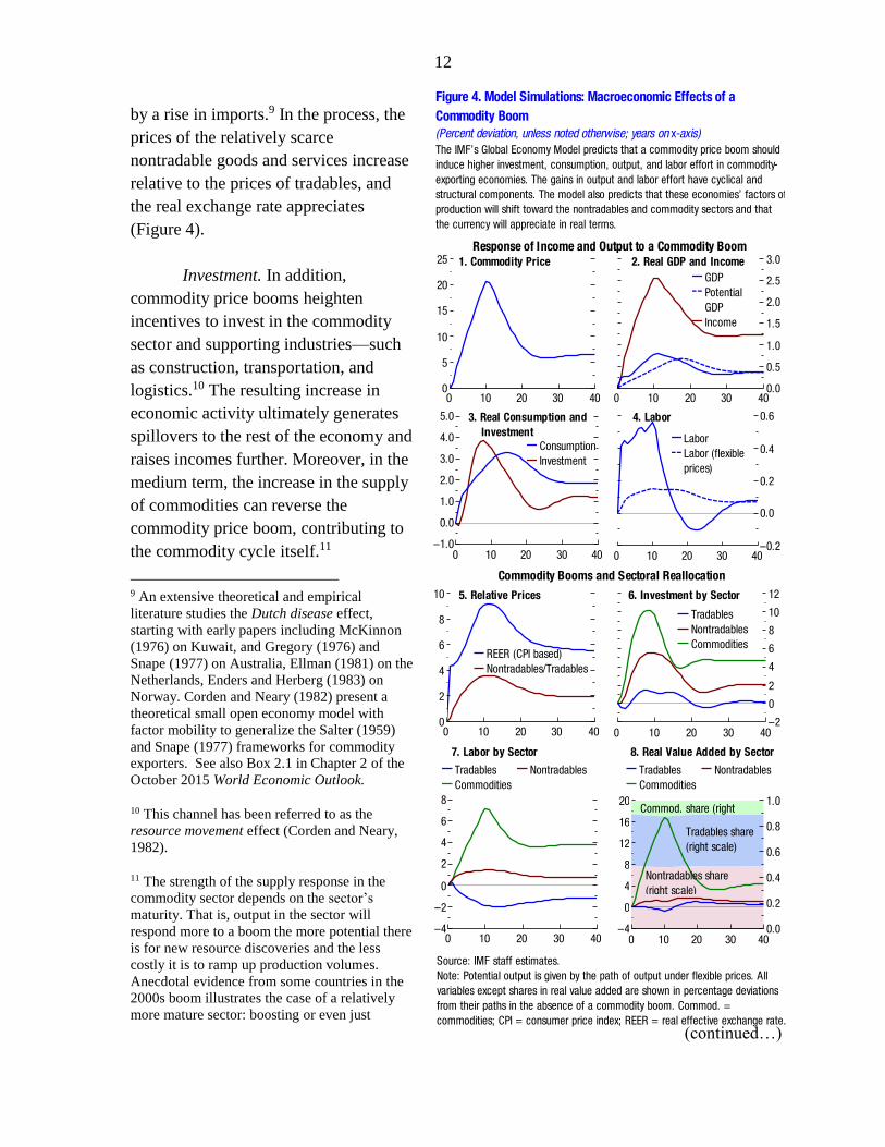
by a rise in imports.9 In the process, the

prices of the relatively scarce

nontradable goods and services increase

relative to the prices of tradables, and

the real exchange rate appreciates

(Figure 4).

Investment. In addition,

commodity price booms heighten

incentives to invest in the commodity

sector and supporting industries—such

as construction, transportation, and

logistics.10 The resulting increase in

economic activity ultimately generates

spillovers to the rest of the economy and

raises incomes further. Moreover, in the

medium term, the increase in the supply

of commodities can reverse the

commodity price boom, contributing to

the commodity cycle itself.11

9 An extensive theoretical and empirical

literature studies the Dutch disease effect,

starting with early papers including McKinnon

(1976) on Kuwait, and Gregory (1976) and

Snape (1977) on Australia, Ellman (1981) on the

Netherlands, Enders and Herberg (1983) on

Norway. Corden and Neary (1982) present a

theoretical small open economy model with

factor mobility to generalize the Salter (1959)

and Snape (1977) frameworks for commodity

exporters. See also Box 2.1 in Chapter 2 of the

October 2015 World Economic Outlook.

10 This channel has been referred to as the

resource movement effect (Corden and Neary,

1982).

11 The strength of the supply response in the

commodity sector depends on the sector’s

maturity. That is, output in the sector will

respond more to a boom the more potential there

is for new resource discoveries and the less

costly it is to ramp up production volumes.

Anecdotal evidence from some countries in the

2000s boom illustrates the case of a relatively

more mature sector: boosting or even just

(continued…)

0

5

10

15

20

25

0 10 20 30 40

–0.2

0.0

0.2

0.4

0.6

0 10 20 30 40–1.0

0.0

1.0

2.0

3.0

4.0

5.0

0 10 20 30 40

0.0

0.5

1.0

1.5

2.0

2.5

3.0

0 10 20 30 40

Source: IMF staff estimates.

Note: Potential output is given by the path of output under flexible prices. All

variables except shares in real value added are shown in percentage deviations

from their paths in the absence of a commodity boom. Commod. =

commodities; CPI = consumer price index; REER = real effective exchange rate.

Figure 4. Model Simulations: Macroeconomic Effects of a

Commodity Boom(Percent deviation, unless noted otherwise; years on x-axis)

2. Real GDP and Income1. Commodity Price

Index

3. Real Consumption and

Investment

4. Labor

GDP

Potential

GDP

Income

–2

0

2

4

6

8

10

12

0 10 20 30 40

–4

–2

0

2

4

6

8

0 10 20 30 40

6. Investment by Sector

Response of Income and Output to a Commodity Boom

Commodity Booms and Sectoral Reallocation

7. Labor by Sector

0

2

4

6

8

10

0 10 20 30 40

–4

0

4

8

12

16

20

0.0

0.2

0.4

0.6

0.8

1.0

0 10 20 30 40

8. Real Value Added by Sector

Labor

Labor (flexible

prices)

Consumption

Investment

5. Relative Prices

REER (CPI based)

Nontradables/Tradables

Tradables Nontradables

Commodities

Tradables

Nontradables

Commodities

Tradables Nontradables

Commodities

Commod. share (right

scale)Tradables share

(right scale)

Nontradables share

(right scale)

The IMF’s Global Economy Model predicts that a commodity price boom should

induce higher investment, consumption, output, and labor effort in commodity-

exporting economies. The gains in output and labor effort have cyclical and

structural components. The model also predicts that these economies’ factors of

production will shift toward the nontradables and commodity sectors and that

the currency will appreciate in real terms.

13

The income and investment channels are interrelated. The income gain in the

domestic economy will be higher and more broadly based if investment and activity in the

commodity sector respond more strongly to the increase in the terms of trade. Likewise, a

greater income windfall will make higher investment more likely.

Additional Factors Affecting the Commodity Cycle

There are numerous other factors that could influence the commodity cycle and its

effect on the commodity-exporting economy. Four such factors are expectations about the

price of the commodity, the reaction of fiscal policy to higher revenues, the easing of

financial frictions due to the commodity boom, and sectoral reallocation of capital and labor.

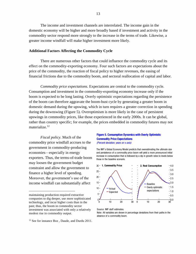
Commodity price expectations. Expectations are central to the commodity cycle.

Consumption and investment in the commodity-exporting economy increase only if the

boom is expected to be long lasting. Overly optimistic expectations regarding the persistence

of the boom can therefore aggravate the boom-bust cycle by generating a greater boom in

domestic demand during the upswing, which in turn requires a greater correction in spending

during the downswing (Figure 5). Overoptimism is more likely in the case of persistent

upswings in commodity prices, like those experienced in the early 2000s. It can be global,

rather than country specific; for example, the prices embedded in commodity futures may not

materialize.12

Fiscal policy. Much of the

commodity price windfall accrues to the

government in commodity-producing

economies—especially in energy

exporters. Thus, the terms-of-trade boom

may loosen the government budget

constraint and allow the government to

finance a higher level of spending.

Moreover, the government’s use of the

income windfall can substantially affect

maintaining production required extractive

companies to dig deeper, use more sophisticated

technology, and incur higher costs than in the

past; thus, the boom in commodity sector

investment was associated with only a relatively

modest rise in commodity output.

12 See for instance Boz , Daude, and Durdu 2011.

0.0

0.5

1.0

1.5

2.0

2.5

3.0

3.5

4.0

0 10 20 300

5

10

15

20

25

30

0 10 20 30

Source: IMF staff estimates.

Note: All variables are shown in percentage deviations from their paths in the

absence of a commodity boom.

Figure 5. Consumption Dynamics with Overly Optimistic

Commodity Price Expectations(Percent deviation; years on x-axis)

2. Real Consumption1. Commodity Price

Index

Baseline

Overly optimistic

expectationsActual

Expected

The IMF’s Global Economy Model predicts that overestimating the ultimate size

and persistence of a commodity price boom will yield a more pronounced initial

increase in consumption that is followed by a dip in growth rates to levels below

those in the baseline scenario.

14

the economy’s response to the commodity price cycle.13 For example, if the government

pursues a procyclical fiscal policy during the boom, using the additional revenues to reduce

taxes on households or increase consumption spending, it can aggravate the boom-bust cycle

in economic activity. In contrast, if the government invests in productivity-enhancing capital

(whether infrastructure or human capital), productive capacity and income can benefit over

the longer term.14

Financial frictions. The commodity boom increases returns, thereby improving

companies’ net worth and reducing their leverage. Reduced leverage, in turn, decreases both

the premium firms pay to obtain financing and their cost of capital. The result is to reduce the

economy’s financial frictions, broadly defined. Increased global risk appetite during the

boom can further magnify this channel. The effect can be illustrated with one summary

measure of the cost of external financing—sovereign bond yield spreads—for a sample of

commodity-exporting economies

from 1997 to 2014 (Figure 6). The

negative relationship between the

country-specific terms of trade and

spreads implies that the cost of

financing decreases for exporters

during commodity booms and

increases during downswings.

The reduction in the cost of

financing and the easing of financial

frictions further boosts income and

potential output during the upswing;

its effects reverse during the

downswing. The effect of the

commodity price cycle on financial

frictions is therefore another channel

that aggravates the boom-bust

dynamics in a commodity-exporting

economy. Such effects are unlikely to

affect the economy beyond the

horizon of the commodity cycle

unless they lead to a sustained

13 See the discussion in Chapter 1 of the October 2015 Fiscal Monitor. 14 See Box 2.2 in Chapter 2 of the October 2015 World Economic Outlook for the implications of such a

scenario using a model calibrated to a low-income developing country.

Figure 6. Sovereign Bond Yield Spreads and the Commodity

Terms of Trade

Sources: Thomson Reuters Datastream; and IMF staff calculations.

Note: Data are for commodity-exporting emerging market and developing

economies for which J.P. Morgan Emerging Markets Bond Index Global (EMBI

Global) spreads are available. See Annex 2.1 for the definition of the

commodity terms-of-trade index.

0

1,000

2,000

3,000

4,000

5,000

6,000

0 20 40 60 80 100 120 140

Cou

ntry

-spe

cific

J.P

. M

orga

n EM

BI G

loba

l spr

eads

(ba

sis

poin

ts)

Country-specific commodity terms of trade (index, 2012 = 100)

During 1997–2014, commodity-exporting economies had lower spreads on

sovereign bond yields when their commodity terms of trade was higher, which

meant lower financing costs during the boom phase of the commodity cycle.

15

improvement in financial sector development.

Sectoral reallocation. The responses to a terms-of-trade boom feature a shift of labor

and capital away from the noncommodity tradables sector toward the commodities and

nontradables sectors as part of the equilibrium adjustment to the windfall. The sectoral

reallocation of factors raises additional issues. If manufacturing is associated with positive

externalities for the broader economy (such as learning-by-doing externalities), the shrinking

of the relative size of the manufacturing sector can raise concerns.15 In addition, the

reallocation could change the weights of the different sectors in the overall economy and thus

affect measured aggregate TFP growth. The case studies in section four of the paper

investigate this issue by examining whether sectoral shifts in activity during commodity

booms have altered aggregate TFP growth.

III. COMMODITY TERMS-OF-TRADE WINDFALLS: EMPIRICAL EVIDENCE

How does actual and potential output respond to commodity windfall gains and

losses? This section analyzes the question empirically, using data for a sample of 52

commodity-exporting emerging market and developing economies. A country is classified as

a commodity exporter (using data available for 1962–2014) if (1) commodities constitute at

least 35 percent of its total exports and (2) net exports of commodities are at least 5 percent

of its gross trade (exports plus imports) on average. A list of the countries and their average

shares of commodity exports over 1960-2014 is provided in Table 1.

In the first step of the empirical analysis, event studies are carried out to shed light on

how actual and potential output growth have behaved during and after prolonged upswings in

the commodity terms of trade. The event study findings provide an overview of the main

regularities in the data. However, event studies do not control for contextual factors (such as

the broader effects of global demand booms that often accompany prolonged upswings in

international commodity prices). Therefore, in the second step, the analysis uses a regression

approach to isolate the impact of changes in the terms of trade by controlling for relevant

contextual factors, such as output growth in trading partners.

The Commodity Terms of Trade

To capture the country-specific impact of global commodity price movements, the

analysis focuses on the commodity terms of trade calculated by weighting the global prices

of individual commodities according to country-specific net export volumes (following Gruss

15 See Box 2.1 in Chapter 2 of the October 2015 World Economic Outlook.

16

2014).16 This approach has two advantages over using the price indices of individual export

commodities or standard terms-of-trade measures. First, few of the non-oil commodity

exporters are so specialized that focusing on the price of a single commodity would be

representative of the changes in their terms of trade. Second, the approach recognizes that

fluctuations in commodity prices affect countries differently depending on the composition

of both their exports and their imports. For instance, despite the upswing in food and raw

materials prices in the 2000s, many agricultural commodity exporters did not experience

terms-of-trade windfalls given the even stronger surge in their oil import bills.

16 Other papers that study the macroeconomic impact of country-specific commodity terms of trade include

Deaton and Miller 1996, Dehn 2000, Cashin, Céspedes, and Sahay 2004, and Céspedes and Velasco 2012.

Table 1. Commodity-Exporting Emerging Market and Developing Economies

Energy Metals Food Raw Materials

Emerging Markets

Algeria 89.2 87.9 0.7 0.5 0.2 37.6

Angola 81.1 47.8 5.5 26.2 3.2 34.6

Argentina 49.8 5.7 1.5 30.0 12.7 20.1

Azerbaijan 76.7 73.2 0.7 0.8 1.9 35.9

Bahrain 60.4 35.5 24.1 0.7 0.1 12.4

Brazil 45.3 3.3 9.5 23.5 8.9 8.3

Brunei Darussalam 90.0 89.9 0.0 0.1 0.0 55.5

Chile 61.2 0.8 48.0 7.0 5.5 20.9

Colombia 58.5 21.7 0.3 34.7 1.9 20.8

Costa Rica 36.2 0.4 0.4 34.9 0.5 8.4

Ecuador 79.0 40.1 0.2 38.8 0.7 32.6

Gabon 78.4 66.3 1.2 0.5 10.8 44.4

Guatemala 45.4 2.4 0.3 36.6 6.1 8.1

Guyana 66.3 0.0 21.5 41.9 2.9 14.4

Indonesia 64.4 40.8 5.0 8.5 10.1 24.9

Iran 81.5 78.9 0.6 0.4 1.6 41.4

Kazakhstan 70.5 53.3 11.7 4.3 1.3 35.5

Kuwait 72.2 71.7 0.1 0.4 0.1 42.4

Libya 96.8 96.7 0.0 0.1 0.0 58.2

Malaysia 45.0 12.7 6.3 8.2 17.8 15.3

Oman 79.8 77.8 1.4 1.0 0.0 42.3

Paraguay 65.4 0.2 0.4 36.6 28.5 12.4

Peru 60.6 7.4 32.8 18.0 2.3 17.5

Qatar 82.5 82.4 0.0 0.1 0.0 49.2

Russia 60.5 50.3 6.6 1.0 2.5 34.0

Saudi Arabia 85.8 85.5 0.1 0.1 0.1 47.3

Syria 54.3 45.8 0.1 2.7 6.2 8.2

Trinidad and Tobago 64.2 60.9 1.2 2.0 0.2 19.8

Turkmenistan 58.9 45.5 0.4 0.2 12.8 19.7

United Arab Emirates 49.6 36.8 13.4 2.4 0.1 12.6

Uruguay 37.0 0.6 0.2 22.5 13.7 5.5

Venezuela 87.1 82.1 4.1 0.8 0.1 46.6

Commodity Exports (Percent of total exports) Net Commodity Exports

(Percent of total

exports-plus-imports)Total Commodities

Extractive Nonextractive

17

For each country, the commodity terms-of-trade indices are constructed as a trade-

weighted average of the prices of imported and exported commodities. The annual change in

country 𝑖’s terms-of-trade index (CTOT) in year 𝑡 is given by:

∆log𝐶𝑇𝑂𝑇𝑖,𝑡 = ∑ ∆log𝑃𝑗,𝑡τ𝑖,𝑗,𝑡𝐽𝑗=1 ,

in which 𝑃𝑗,𝑡 is the relative price of commodity 𝑗 at time 𝑡 (in U.S. dollars and divided by the

IMF’s unit value index for manufactured exports) and ∆ denotes the first difference. Country

𝑖’s weights for each commodity price, τ𝑖,𝑗,𝑡, are given by

τ𝑖,𝑗,𝑡 =𝑥𝑖,𝑗,𝑡−1−𝑚𝑖,𝑗,𝑡−1

∑ 𝑥𝑖,𝑗,𝑡−1𝐽𝑗=1 +∑ 𝑚𝑖,𝑗,𝑡−1

𝐽𝑗=1

,

in which 𝑥𝑖,𝑗,𝑡−1 (𝑚𝑖,𝑗,𝑡−1) denote the average export (import) value of commodity 𝑗 by

country 𝑖 between 𝑡 − 1 and 𝑡 − 5 (in U.S. dollars). This average value of net exports is

Table 1. Commodity-Exporting Emerging Market and Developing Economies (concluded)

Energy Metals Food Raw Materials

Low-Income Developing Countries

Bolivia 65.9 25.3 27.7 6.0 6.8 28.4

Cameroon 71.3 16.1 6.6 34.7 13.9 22.6

Chad 91.6 4.5 0.0 15.6 71.5 8.6

Republic of Congo 61.3 52.6 0.2 1.8 6.7 30.6

Côte d'Ivoire 70.9 11.9 0.2 44.7 14.0 26.7

Ghana 66.0 5.4 7.0 50.2 3.3 12.3

Guinea 67.3 0.5 61.4 3.9 1.5 9.3

Honduras 66.6 1.3 2.8 60.0 2.5 14.1

Mauritania 75.9 9.2 47.2 23.8 0.0 12.2

Mongolia 59.2 4.6 35.6 1.9 17.2 12.4

Mozambique 46.1 4.7 26.7 10.9 3.9 5.1

Myanmar 52.8 36.1 0.7 6.1 9.8 24.4

Nicaragua 55.9 0.6 0.5 42.7 12.2 7.2

Niger 65.8 2.1 38.0 23.2 2.5 10.2

Nigeria 88.4 79.5 0.7 6.2 2.0 46.8

Papua New Guinea 58.0 6.7 24.5 20.7 6.1 15.7

Sudan 69.4 56.5 0.3 11.8 9.8 11.3

Tajikistan 63.4 0.0 51.6 0.2 11.6 21.5

Yemen 82.5 79.6 0.2 2.4 0.4 20.8

Zambia 77.0 0.4 72.4 2.7 1.6 30.4

Memorandum

Number of Economies 52 52 52 52 52 52

Maximum 96.8 96.7 72.4 60.0 71.5 58.2

Mean 67.1 34.6 11.6 14.5 6.7 24.2

Median 65.9 30.4 1.3 6.2 2.7 20.8

Standard Deviation 14.5 32.6 18.2 16.5 11.0 14.5

Sources: UN Comtrade; and IMF staff calculations.

Note: Countries listed are those for which gross commodity exports as a share of total exports were greater than 35 percent and net commodity exports as a share of total trade

(exports plus imports) were greater than 5 percent, on average, between 1962 and 2014. Commodity intensities are determined using a breakdown of the first criterion into the four

main commodity categories: energy, food, metals, and raw materials.

Commodity Exports (Percent of total exports) Net Commodity Exports

(Percent of total

exports-plus-imports)Total Commodities

Extractive Nonextractive

18

divided by total commodity trade

(exports plus imports of all

commodities, averaged over 𝑡 − 1 and

𝑡 − 5).

The commodity price series

start in 1960. Prices of 41 commodities

are used, sorted into four broad

categories:

1. Energy: coal, crude oil, and

natural gas;

2. Metals: aluminum, copper, iron

ore, lead, nickel, tin, and zinc;

3. Food: bananas, barley, beef,

cocoa, coconut oil, coffee,

corn, fish, fish meal,

groundnuts, lamb, oranges,

palm oil, poultry, rice, shrimp,

soybean meal, soybean oil,

soybeans, sugar, sunflower oil,

tea, and wheat;

4. Raw materials: cotton,

hardwood logs and sawn wood,

hides, rubber, softwood logs

and sawn wood, soybean meal,

and wool.

The price of crude oil is the simple

average of three spot prices: Dated

Brent, West Texas Intermediate, and

Dubai Fateh. The World Bank’s

Global Economic Monitor database

has been used to extend the price

series of barley, iron ore, and natural

gas from the IMF’s

Primary Commodity Prices System

back to 1960. The price of coal is the

Australian coal price, extended back to

0

20

40

60

80

100

120

1960 65 70 75 80 85 90 95 2000 05 10 14

Sources: Gruss 2014; IMF, Primary Commodity Price System; U.S. Energy

Information Administration; World Bank, Global Economic Monitor database;

and IMF staff calculations.

Note: The definition of the commodity terms of trade is given in Annex 2.1.

The algorithm for selecting the cycles is described in Annex 2.2. The portion

of a cycle before (after) the peak is referred to as an upswing (downswing).

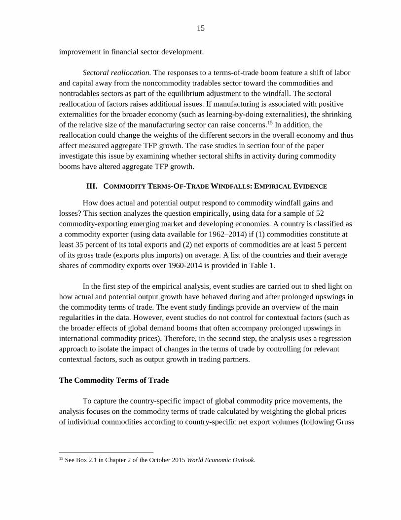
Figure 7. Identification of Cycles in the Commodity Terms of

Trade: Three Country Examples(Index, 2012 = 100)

1. Saudi Arabia (Energy exporter)

Commodity terms of trade (moving average) Cycle

Selected peaks

0

20

40

60

80

100

120

140

1960 65 70 75 80 85 90 95 2000 05 10 14

2. Chile (Metals exporter)

0

50

100

150

200

250

300

1960 65 70 75 80 85 90 95 2000 05 10 14

3. Ghana (Food exporter)

The event studies focus on the behavior of variables during commodity terms-

of-trade cycles with prolonged upswings that peaked before 2000. On

average, those upswings were eight years long for exporters of extractive

commodities and five years long otherwise, and the commodity terms of trade

improved by 63 percent.

19

1960 using the World Bank’s Global

Economic Monitor database and U.S.

coal price data from the U.S. Energy

Information Administration.

Since the recent declines in

commodity prices have occurred after

an unusually prolonged boom phase,

the event studies focus on past

episodes of persistent upswings in the

commodity terms of trade. A modified

version of the Bry-Boschan Quarterly

algorithm (standard in the business

cycle literature; Harding and Pagan

2002) is used to identify commodity

price cycles, which were similar to the

most recent cycle (Figure 7 presents

three examples). In particular, the

algorithm as used here differs from

the standard version in two ways: (1)

it is applied to a smoothed (five-year

centered moving-average) version of

the price index because the underlying

series are choppy, making it difficult

for standard algorithms to identify

meaningful cycles, and (2) it allows

for asymmetry between upswings and

downswings, as the focus here is on

cycles in which the upswing was at

least five years long, even if the

subsequent downswing was sudden.

By contrast, most existing studies

have focused on price changes of at

least a given magnitude, rather than a

given duration, and on samples of

disjointed price increases or

decreases, rather than full cycles that

include an upswing and a downswing

phase.

0

50

100

150

200

250

300

350

400

0 2 4 6 8 10 12 14 16 18 20

Trou

gh-t

o-pe

ak in

crea

se in

com

mod

ity p

rice

inde

x (p

erce

nt)

Duration of upswings (years)

–20

–10

0

10

20

30

40

50

60

1 2 3 4 5 6 7 8 9 10 11 12 13 14 15 16 17 18

Figure 8. Characteristics, Amplitudes, and Durations of Cycles

1. Frequency of Upswings and Downswings of Given Durations

(Percent; years on x-axis)

Upswings

Downswings

0

24

68

1012

1416

18

1960 65 70 75 80 85 90 95 2000 05 10 14

2. Number of Peaks in Each Year, by Commodity Type

–100

–80

–60

–40

–20

0

20

0 2 4 6 8 10 12 14 16 18 20

Peak

-to-

trou

gh d

ecre

ase

in

com

mod

ity p

rice

inde

x (p

erce

nt)

Duration of downswings (years)

Energy

Food

Metals

Raw materials

3. Price Increases by Duration of Upswing

4. Price Decreases by Duration of Downswing

Sources: Gruss 2014; IMF, Primary Commodity Price System; U.S. Energy

Information Administration; World Bank, Global Economic Monitor database;

and IMF staff calculations.

Note: The cycles shown are for the country-specific commodity terms-of-

trade indices. See Annexes 2.1 and 2.2 for the data definitions and cycle-

dating methodology.

20

The algorithm identifies 115

cycles since 1960 (78 with peaks before

2000 and 37 with peaks after 2000).

There are approximately two cycles a

country. Upswings are slightly longer

than downswings, with a mean (median)

of seven (six) years for upswings and six

(five) years for downswings (Figure 8,

panel 1). The duration of phases and the

amplitude of price movements are

correlated (Figure 8, panels 3 and 4).

Most peaks were in the 1980s and the

most recent years, particularly for

extractive commodities (Figure 8, panel

2).17

Event Studies of Commodity Cycles

with Pre-2000 Peaks

Event studies are carried out for

the cycles with peaks before 2000, where

the full downswing has been observed

already (the end of the downswing phase

cannot yet be identified for the post-2000

upswings). Average growth rates over

upswings (downswings) are computed by

first averaging for a given country over

all upswing (downswing) years, then

taking simple averages of these across

countries.18

The event studies confirm that

output and domestic spending tend to

grow faster during upswings in

17 Upswings are defined trough to peak

(excluding the trough year, but including the

peak year); downswings are defined peak to

trough (excluding the peak year, but including

the trough year).

18 Samples are fully balanced, that is, they include the same country cycles for upswings and downswings.

–4–2

02468

101214

Government

spending

Real

credit

REER

(all)

REER

(fixed)

REER

(flexible)

CPI

inflation

0

4

8

12

16

20

GDP Consumption Private

investment

Public

investment

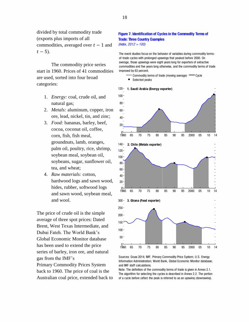
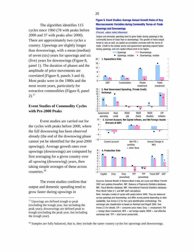
Figure 9. Event Studies: Average Annual Growth Rates of Key

Macroeconomic Variables during Commodity Terms-of-Trade

Upswings and Downswings

(Percent, unless noted otherwise)

Sources: External Wealth of Nations Mark II data set (Lane and Milesi -Ferretti

2007 and updates thereafter); IMF, Balance of Payments Statistics database;

IMF, Fiscal Monitor database; IMF, International Financial Statistics database;

Penn World Table 8.1; and IMF staff calculations.

Note: Samples consist of cycles with peaks before 2000. They are balanced

across upswings and downswings, but differ across panels depending on data

availability. See Annex 2.2 for the cycle identification methodology. The

exchange rate classification is based on Reinhart and Rogoff 2004. See

Annex 2.3 for details. CPI = consumer price index; Emp. = employment; FDI

= foreign direct investment; NFA = net foreign assets; REER = real effective

exchange rate; TFP = total factor productivity.

Upswings Downswings

Upswings, median Downswings, median

1. Expenditure Side

2. Real Government Spending, Private Credit,

Exchange

–2–1

0123456

Capital Emp. Emp.

(smoothed)

TFP TFP

(smoothed)

Trend GDP GDP

4. Production Side

–10

–5

0

5

10

Current account Net FDI +

portfolio

+ other flows

Annual Change in

NFA

3. Current Account, Net Capital Inflows, and Net Foreign Assets

(Percent of GDP)

Output and domestic spending tend to grow faster during upswings in the

commodity terms of trade than in downswings. The growth of trend output

tends to vary as well, as capital accumulation comoves with the terms of

trade. Credit to the private sector and government spending expand faster

during upswings, and net capital inflows tend to be higher.

21

commodity terms of trade than in downswings. The variation in investment growth—both

private and public—is particularly pronounced (Figure 9, panel 1). During upswings, real

GDP has grown about 1.5 percentage points more per year than in downswings, real

consumption about 2.0 to 2.5 percentage points more, and investment about 8.0 to

8.5 percentage points more. Differences are statistically significant at the 5 percent level for

all of these variables. Investment and consumption contribute about equally to the difference

in the growth of real GDP, as the stronger response of investment makes up for its smaller

share in overall spending.

Factors supporting domestic demand, such as credit to the private sector and overall

government spending, tend to expand more strongly in upswings than in downswings, and

differences for government spending are significant at the 5 percent level (Figure 9, panel

2).19

Somewhat surprisingly, the real effective exchange rate in the identified episodes did

not appreciate during the average pre-2000 upswing (differences between upswings and

downswings are not significant at conventional levels). This pattern, however, holds only for

the cycles with peaks before 2000. During the pre-2000 upswings, factors other than the

commodity terms of trade appear to have dominated the movements in the real exchange

rate. By contrast, the most recent upswing is more in line with priors, showing about 2.0 to

2.5 percent average real appreciation per year. However, even before 2000, breaking the

sample into episodes involving countries with fixed versus flexible exchange rate regimes

reveals that flexible regimes have been associated with currency appreciations during

upswings (and depreciations during downswings), as would be expected, whereas

depreciations have occurred in fixed regimes during both upswings and downswings.

The behavior of external accounts provides some additional evidence that financing

constraints loosen during upswings. Even though outflows in the form of official reserves

and foreign direct investment rise when commodity prices are high, net commodity exporters

have received, on average, slightly higher net capital inflows during upswings than during

downswings (Figure 9, panel 3). Given the higher net inflows, no general tendency toward

improved net foreign asset positions has been observed for upswings, even though, as

expected, current account balances have been stronger in those episodes. Specifically, the

average ratio of net foreign assets to GDP has tended to rise during upswings, a result driven

by a few oil exporters, while the median ratio has tended to decline more in upswings than in

downswings.

19 Husain, Tazhibayeva, and Ter-Martirosyan (2008) examine a sample of 10 oil exporters and find that oil price

changes affect the economic cycle only through their impact on fiscal policy. Their results are particularly stark

for Gulf Cooperation Council countries, in which all oil income accrues to the state.

22

A growth-accounting perspective highlights the key supply-side factors behind the

cycle in output growth. Aggregate production factors (capital and labor) and TFP have

tended to move in tandem with the changes in the commodity terms of trade (Figure 9, panel

4). The comovement is particularly strong for the rate of change in the capital stock

(significant at the 10 percent level), which is consistent with the substantially faster growth in

investment spending during upswings. TFP growth is also significantly different between

upswings and downswings (at the one percent level), though as it is measured as a Solow

residual, this could be capturing cyclicality in utilization rates or hours worked. The variation

in employment growth is much smaller, not statistically significant, and is driven by Latin

America, where employment has grown 1.5 percentage points more during upswings than in

downswings.

The growth rate of trend output—calculated using estimates of the actual capital stock

and smoothed employment and TFP series—is considerably smoother than that of actual

output. Trend output growth weakens during downswings relative to upswings, but it does so

with less vigor than actual output growth. Annual actual output growth tended to be 1.0 to

1.5 percentage points higher on average during upswings than in downswings, whereas

potential output growth tended to be only 0.3 to 0.5 percentage point higher.20 The fact that

inflation tends to be higher during upswings than in downswings (Figure 9, panel 2)

corroborates the notion of a smaller amount of slack in the economy during upswings.

20 Employment and TFP are smoothed using a standard Hodrick-Prescott filter on annual data; the capital and

labor shares are from Penn World Table 8.1.

23

The exchange rate regime, cyclicality of fiscal policy, and depth of financial markets

have a bearing on the difference in

growth between upswings and

downswings (Figure 10). Countries

with fixed exchange rates

experience slightly stronger

variation in growth relative to

countries with flexible exchange

rates. This is consistent with the

notion that a more flexible exchange

rate tends to act as a shock absorber

and cushion the domestic effects of

terms-of-trade shocks, though

differences are not significant at

conventional levels.21 The difference

in the growth rate of output between

upswings and downswings is larger

in countries with more procyclical

fiscal spending, and this is

significant at the one percent level.22

Countries with a lower level of

credit to the private sector (relative

to GDP) also exhibit stronger

variation in growth, and again this is

statistically significant at the one

percent level.23 The growth

slowdown in these countries is

21 Exchange rate regimes are categorized as fixed or flexible according to the classification set out by Reinhart

and Rogoff (2004). Regimes of countries in their coarse categories 1 and 2 are classified as fixed, and those in

their coarse categories 3 and 4 are categorized as flexible. Countries in categories 1 and 2 have no separate legal

tender or variously use currency boards, pegs, horizontal bands, crawling pegs, and narrow crawling bands.

Countries in categories 3 and 4 variously have wider crawling bands, moving bands, and managed floating or

freely floating arrangements. As very few countries maintain the same regime over an entire cycle, the

exchange rate regime in the peak year is used to classify the cycle. The sample includes 34 cycles with fixed

exchange rates but only 8 cycles with flexible exchange rates. Regimes classified as free-falling are dropped.

22 As some correlation between fiscal spending and commodity prices may be optimal, cycles are classified here

as having more procyclical fiscal policy if the correlation between the growth of real spending and the change in

the commodity terms of trade is greater than the sample median.

23 Cycles are classified as having a high (low) ratio of credit to GDP depending on whether average domestic

credit to the private sector as a share of GDP during the upswing is above (below) the sample median.

0.0

0.5

1.0

1.5

2.0

2.5

3.0

3.5

4.0

4.5

Fixed

exchange

rate

Flexible

exchange

rate

High

fiscal

pro-

cyclicality

Low

fiscal

pro-

cyclicality

Low

credit-

to-GDP

ratio

High

credit-

to-GDP

ratio

Figure 10. Variation in Average Output Growth between Upswings

and Downswings: The Role of Policy Frameworks and Financial

Depth

(Percentage points)

Sources: IMF, Fiscal Monitor database; IMF, International Financial Statistics

database; Penn World Table 8.1; and IMF staff calculations.

Note: The bars (blocks) show the difference between the average (median)

growth rates during upswings and subsequent downswings. The exchange rate

regime classification is based on Reinhart and Rogoff 2004. See Annex 2.3 for

details. An episode is classified as having high fiscal policy procyclicality if the

correlation between real government spending growth and the change in the

smoothed net commodity terms of trade during the cycle is higher than the

overall sample median (and having low fiscal policy procyclicality otherwise). A

country is classified as having a high credit-to-GDP ratio if credit to the private

sector (as a share of GDP) during the upswing is higher than the sample

median (and having a low credit-to-GDP ratio otherwise).

Difference in means Difference in medians

Commodity-exporting countries with more flexible exchange rates, less

procyclical fiscal policy, and a higher level of credit to the private sector exhibit

less growth variation over commodity price cycles.

24

sharper during downswings, probably because they experience a greater tightening of

borrowing constraints when commodity prices decline than do countries with greater

financial depth.24

Commodity exporters differ

across many other dimensions—in

terms of the weight of commodities

in their aggregate production, the

nature of the commodities they

export (for example, exhaustible

versus renewable resource bases),

and their levels of economic and

institutional development. Among

the commodity-exporting countries,

emerging market economies can be

differentiated from low-income

developing countries along four key

dimensions: commodity intensity,

exchange rate regime, credit ratio,

and fiscal procyclicality (Figure 11).

Emerging markets tend to have a

greater degree of commodity

intensity (GDP share of gross

commodity exports). A greater share

of low-income developing countries

operate fixed exchange rates.

Emerging markets tend to have

greater financial depth, as captured

by higher credit-to GDP ratios. And

emerging markets tend to have a

more procyclical fiscal stance (Figure 11).

As could be expected, the growth patterns described previously are more marked for

economies that are less diversified, that is, those in which commodity exports account for a

larger share of GDP. They are also clearer for exporters of extractive commodities, whose

economies tend to be less diversified and face more persistent commodity terms-of-trade

24 This result is not driven by the variation in the level of economic development, which tends to be correlated

with financial depth.

0

10

20

30

40

50

60

70

80

EMs LIDCs EMs LIDCs EMs LIDCs EMs LIDCs

Figure 11. Commodity Intensity, Policy Frameworks, and Financial

Depth: Commodity-Exporting Emerging Markets versus Low-

Income Developing Countries(Percent)

Sources: IMF, Fiscal Monitor database; IMF, International Financial Statistics

database; World Bank, World Development Indicators; and IMF staff

calculations.

Note: Figures are the averages of data for all available years across all

commodity exporters within each group. EM = emerging market; LIDC = low-

income developing country. 1Average of commodity exports as a share of GDP.2Share of commodity-exporting emerging markets and low-income developing

countries with a fixed exchange rate regime as defined in Annex 2.3.3Average of bank credit to the private sector as a share of GDP.4Determined by whether the correlation between real spending growth and the

change in the smoothed commodity terms of trade is greater or less than the

sample median.

Fixed exchange

rate regime2

Credit-to-GDP

ratio3

Fiscal

procyclicality4

Commodity

intensity1

25

cycles. Low-income countries have less

procyclical fiscal spending and a slightly

lower degree of commodity intensity in

production but also less flexible exchange rates

and lower levels of financial development.

They exhibit greater variability in their

growth rates for investment,

employment, and TFP compared with

emerging market economies, but the

differences between the two groups are

not statistically significant (Figure 12).

The Boom of the 2000s

The event studies of commodity

price cycles with pre-2000 peaks provide

evidence that is highly relevant for the

current downswing in commodity

exporters. Nevertheless, the most recent

commodity price boom was different in a

number of dimensions from the earlier booms.

In particular, this boom entailed a larger

upswing in the terms of trade, especially

for commodity exporters specializing in

energy and metals.25 There were also a

greater number of oil exporters in the

recent upswing, for reasons of data

availability or more recent oil discovery

and development.

25 For the sample of net exporters that

experienced at least two upswings in our data

sample—one in the 2000s and at least one in

the 1960–99 period—the cumulative net terms-

of-trade increase averaged slightly more than 70

percent in the 2000s, compared with 50 percent

in past episodes. When all net exporters—not

only those that recorded a pre-2000s upswing—

are included, the average cumulative increase in

the commodity terms of trade in the 2000s was

even sharper, about 140 percent.

–0.5

0.0

0.5

1.0

1.5

2.0

2.5

Capital Employment TFP Trend GDP

0

2

4

6

8

10

12

14

GDP Consumption Private

investment

Public

investment

Figure 12. Average Differences in Real Growth Rates between

Upswings and Downswings

(Percentage points)

Sources: IMF, Fiscal Monitor database; Penn World Table 8.1; and IMF staff

calculations.

Note: The bars show the average differences between growth rates during

upswings and downswings. EM = emerging market; LIDC = low-income

developing country; TFP = total factor productivity.

EMs (means) LIDCs (means)

EMs (medians) LIDCs (medians)

Emerging Markets and Low-Income Developing Countries

Extractive and Nonextractive Commodity Exporters

0

2

4

6

8

10

12

14

GDP Consumption Private

investment

Public

investment

–1.0

–0.5

0.0

0.5

1.0

1.5

2.0

2.5

3.0

Capital Employment TFP Trend GDP

Extractive (means) Nonextractive (means)

Extractive (medians) Nonextractive (medians)

3. Expenditure Side

4. Production Side

1. Expenditure Side

2. Production Side

26

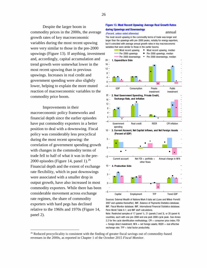
Despite the larger boom in

commodity prices in the 2000s, the average annual

growth rates of key macroeconomic

variables during the most recent upswing

were very similar to those in the pre-2000

upswings (Figure 13). If anything, investment

and, accordingly, capital accumulation and

trend growth were somewhat lower in the

most recent upswing than in previous

upswings. Increases in real credit and

government spending were also slightly

lower, helping to explain the more muted

reaction of macroeconomic variables to the

commodity price boom.

Improvements in their

macroeconomic policy frameworks and

financial depth since the earlier episodes

have put commodity exporters in a better

position to deal with a downswing. Fiscal

policy was considerably less procyclical

during the most recent upswing: the

correlation of government spending growth

with changes in the commodity terms of

trade fell to half of what it was in the pre-

2000 episodes (Figure 14, panel 1).26

Financial depth and the extent of exchange

rate flexibility, which in past downswings

were associated with a smaller drop in

output growth, have also increased in most

commodity exporters. While there has been

considerable movement across exchange

rate regimes, the share of commodity

exporters with hard pegs has declined

relative to the 1960s and 1970s (Figure 14,

panel 2).

26 Reduced procyclicality is consistent with the finding of greater fiscal savings out of commodity-based

revenues in the 2000s, as reported in Chapter 1 of the October 2015 Fiscal Monitor.

–5

0

5

10

Current account Net FDI + portfolio +

other flows

Annual change in NFA

–5

0

5

10

Capital Employment TFP Trend GDP

–4

0

4

8

12

16

20

Government

spending

Real credit REER CPI inflation

–4

0

4

8

12

16

20

GDP Consumption Private

investment

Public

investment

Figure 13. Most Recent Upswing: Average Real Growth Rates

during Upswings and Downswings

(Percent, unless noted otherwise)

Sources: External Wealth of Nations Mark II data set (Lane and Milesi -Ferretti

2007 and updates thereafter); IMF, Balance of Payments Statistics database;

IMF, Fiscal Monitor database; IMF, International Financial Statistics database;

Penn World Table 8.1; and IMF staff calculations.

Note: Restricted samples of 17 (panel 1), 21 (panels 2 and 3), or 20 (panel 4)

countries, each with one pre-2000 and one post-2000 cycle peak. See Annex

2.2 for the cycle identification methodology. CPI = consumer price index; FDI

= foreign direct investment; NFA = net foreign assets; REER = real effective

exchange rate; TFP = total factor productivity.

Most recent upswing Most recent upswing, median

Pre-2000 upswings Pre-2000 upswings, median

Pre-2000 downswings Pre-2000 downswings, median

1. Expenditure Side

2. Real Government Spending, Private Credit,

Exchange Rate, and Inflation

4. Production Side

3. Current Account, Net Capital Inflows, and Net Foreign Assets

(Percent of GDP)

The most recent upswing in the commodity terms of trade was longer and

larger than the upswings with pre-2000 peaks, notably for energy exporters,

but it coincided with average annual growth rates in key macroeconomic

variables that were similar to those in the earlier booms.

27

Commodity exporters are entering the current downswing with stronger external

positions as well. The median annual current account balance and the average annual change

in the net foreign asset position were 5 percentage points of GDP stronger in the 2000s

upswings than earlier.

In summary, the larger

increase in commodity prices in the

2000s could potentially presage

sharper terms-of-trade downswings

for some commodity exporters

(beyond the decline already

experienced) and therefore lead to

sharper reductions in actual and

potential growth. At the same time,

stronger external positions, more

robust policy frameworks, and more

developed financial markets are

likely to help mitigate some of the

growth impacts.

Regression Analysis

This subsection examines the responses of key macroeconomic variables to changes

in the commodity terms of trade.

The estimations of baseline impulse responses presented in the paper follow the local

projection method proposed by Jordà (2005) and developed further by Teulings and Zubanov

(2014). This method provides a flexible alternative to traditional vector autoregression

techniques and is robust to misspecification of the data-generating process. Local projections

use separate horizon-specific regressions of the variable of interest (for example, output,

investment, capital) on the shock variable (in our analysis, the commodity terms of trade) and

a series of control variables. The sequence of coefficient estimates for the various horizons

provides a nonparametric estimate of the impulse-response function.

The local projection method estimates the following equation:

Figure 14. Policies during the 2000s Boom

0.00

0.05

0.10

0.15

0.20

0.25

0.30

0.35

0.40

0.45

1970s 1980s 1990s 2000s

1. Fiscal pro-cyclicality over time

(correlation between changes in the smoothed commodity

terms of trade and real spending growth)

0

10

20

30

40

50

60

70

80

1960s 1970s 1980s 1990s 2000s

2. Share of commodity exporters with hard pegs

(classification based on Reinhart and Rogoff 2004)

28

∆ℎ𝑦𝑖,𝑡 = 𝛼𝑖ℎ + 𝛾𝑡

ℎ + 𝛽ℎ∆𝑠𝑖,𝑡 +∑𝛽1ℎ∆𝑠𝑖,𝑡−𝑗

𝑝

𝑗=1

+∑𝛽2ℎ∆𝑠𝑖,𝑡+ℎ−𝑗

ℎ−1

𝑗=1

+∑𝜃1ℎ∆𝑦𝑖,𝑡−𝑗

𝑝

𝑗=1

+∑𝜃2ℎ𝑥𝑖,𝑡−𝑗

𝑝

𝑗=0

+∑𝜃3ℎ𝑥𝑖,𝑡+ℎ−𝑗

ℎ−1

𝑗=1

+ 𝜀𝑖,𝑡ℎ

where the i subscripts index countries; the t subscripts index years; the h superscripts index

the horizon of the projection after time t; p is the number of lags for each variable; 𝑦𝑖,𝑡 is the

natural logarithm of the variable of interest (for example, output); and 𝑠𝑖,𝑡 is the natural

logarithm of the commodity terms of trade, the shock variable of interest:

∆ℎ𝑦𝑖,𝑡 ≡ 𝑦𝑖,𝑡+ℎ − 𝑦𝑖,𝑡−1

∆𝑠𝑖,𝑡 ≡ 𝑠𝑖,𝑡 − 𝑠𝑖,𝑡−1

𝑦𝑖,𝑡 ≡ ln(𝐺𝐷𝑃𝑖,𝑡); 𝑠𝑖,𝑡 ≡ ln(𝐶𝑇𝑜𝑇𝑖,𝑡)

The equation also includes controls for additional factors, 𝑥𝑖,𝑡, such as the trade-weighted

output growth of trading partners, political regime transition, and conflict in the domestic

economy. Regressions include country fixed effects, α𝑖ℎ, as well as time fixed effects, γ

𝑡ℎ to

control for common economic developments facing all countries in a given year. 𝛽1ℎ is the

contribution to the cumulative increase in (i.e., the level of) 𝑦𝑖,𝑡 at horizon h from a 1

percentage point increase in ∆𝑠𝑖,𝑡 in year t:

𝜕∆ℎ𝑦𝑖,𝑡𝜕∆𝑠𝑖,𝑡

= 𝛽ℎ

A balanced panel for the period 1960–2007 is used for the baseline regression. The period of

the global financial crisis and its aftermath is thus omitted. However, because of differences

in data availability, the number of economies included differs by variable. For example, for

real GDP, the sample spans 32 commodity-exporting emerging market and developing

economies (Table 2).

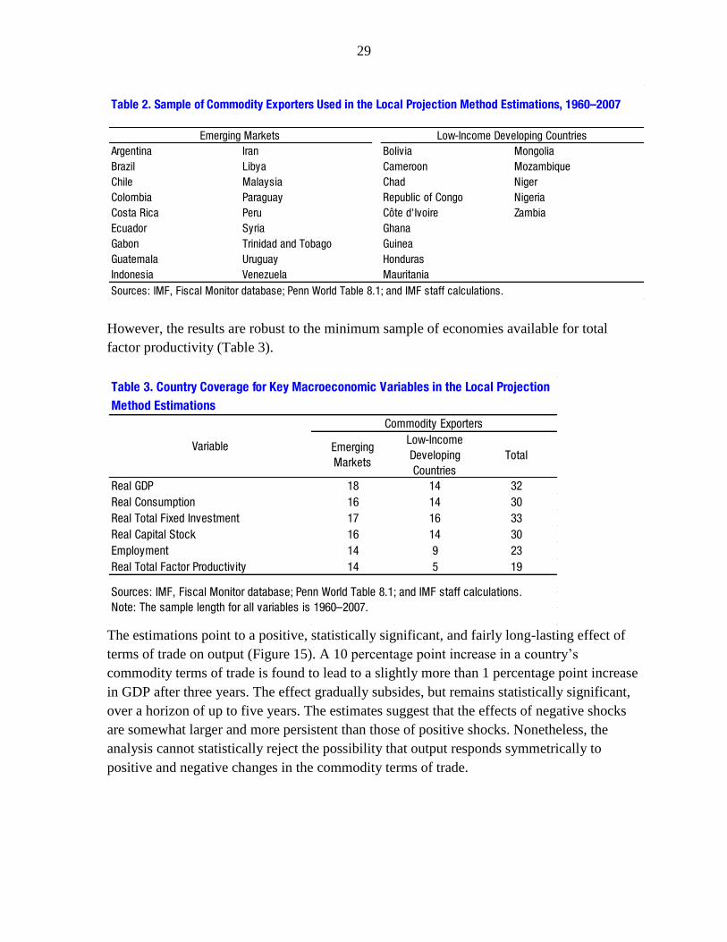
29

However, the results are robust to the minimum sample of economies available for total

factor productivity (Table 3).

The estimations point to a positive, statistically significant, and fairly long-lasting effect of

terms of trade on output (Figure 15). A 10 percentage point increase in a country’s

commodity terms of trade is found to lead to a slightly more than 1 percentage point increase

in GDP after three years. The effect gradually subsides, but remains statistically significant,

over a horizon of up to five years. The estimates suggest that the effects of negative shocks

are somewhat larger and more persistent than those of positive shocks. Nonetheless, the

analysis cannot statistically reject the possibility that output responds symmetrically to

positive and negative changes in the commodity terms of trade.

Argentina Iran Bolivia Mongolia

Brazil Libya Cameroon Mozambique

Chile Malaysia Chad Niger

Colombia Paraguay Republic of Congo Nigeria

Costa Rica Peru Côte d'Ivoire Zambia

Ecuador Syria Ghana

Gabon Trinidad and Tobago Guinea

Guatemala Uruguay Honduras

Indonesia Venezuela Mauritania

Emerging Markets Low-Income Developing Countries

Table 2. Sample of Commodity Exporters Used in the Local Projection Method Estimations, 1960–2007

Sources: IMF, Fiscal Monitor database; Penn World Table 8.1; and IMF staff calculations.

Emerging

Markets

Low-Income

Developing

Countries

Total

Real GDP 18 14 32

Real Consumption 16 14 30

Real Total Fixed Investment 17 16 33

Real Capital Stock 16 14 30

Employment 14 9 23

Real Total Factor Productivity 14 5 19

Table 3. Country Coverage for Key Macroeconomic Variables in the Local Projection

Method Estimations

Sources: IMF, Fiscal Monitor database; Penn World Table 8.1; and IMF staff calculations.

Note: The sample length for all variables is 1960–2007.

Variable

Commodity Exporters

30

Turning to the spending side, both

consumption and investment respond

positively and with statistical significance

to commodity terms-of-trade shocks over a

seven-year period. The average response of

total fixed investment is almost double that

of consumption. The positive response of

public investment is more immediate and

long lasting than that of private investment.

On the production side, shocks to

the commodity terms of trade raise capital

accumulation over the medium term in line

with the estimated persistent response of

investment. The capital stock increases (or

decreases) steadily for seven years after the

shock by a cumulative 1 percentage point.

In contrast, the impacts on labor supply and

TFP are muted. The response of

employment is not statistically significant.

The impact on TFP is only weakly

significant in the first two years after the

shock, which could reflect a cyclical

deterioration in the Solow residual relative

to its underlying trend, as seen in the event

studies. Overall, these results are consistent

with the event study findings, which

suggest that commodity terms-of-trade

shocks affect potential output mainly by

raising capital accumulation.27

27 The estimation does not distinguish between

supply-driven and demand-driven changes in the

commodity terms of trade. Chapter 3 of the April

2012 World Economic Outlook finds the output

responses to demand-driven commodity price

shocks to be somewhat larger than the responses to

supply-driven shocks, but with no statistically

significant difference.

–0.5

0.0

0.5

1.0

1.5

2.0

2.5

–1 0 1 2 3 4 5 6 7

–2

0

2

4

6

8

10

12

14

–1 0 1 2 3 4 5 6 7

–10123456789

–1 0 1 2 3 4 5 6 7–0.5

0.00.51.0

1.52.0

2.53.0

3.54.0

–1 0 1 2 3 4 5 6 7

–2

–1

0

1

2

3

4

5

6

–1 0 1 2 3 4 5 6 7

Source: IMF staff estimates.

Note: t = 0 is year of the shock; dashed lines and shaded areas denote 90

percent confidence bands. In panels 1 and 3–8, solid lines represent the

response of the variable to an exogenous 10 percentage point increase in the

commodity terms of trade. In panel 2, the blue (red) solid line denotes the

response to an exogenous positive (negative) 10 percentage point change in

the commodity terms of trade. In panel 5, the blue (red) solid line denotes the

response of public (private) investment. See Annex 2.4 for the estimation

methodology.

Figure 15. Macroeconomic Variables in the Aftermath of

Commodity Terms-of-Trade Shocks

(Percentage points; years on x-axis)

2. Output (Positive

and negative commodity

terms-of-trade shocks)

1. Output

3. Consumption 4. Investment

–0.5

0.0

0.5

1.0

1.5

2.0

2.5

–1 0 1 2 3 4 5 6 7

–0.6

–0.4

–0.2

0.0

0.2

0.4

0.6

–1 0 1 2 3 4 5 6 7

5. Public and Private

Investment

6. Capital Stock

7. Employment

–1.0

–0.5

0.0

0.5

1.0

1.5

2.0

–1 0 1 2 3 4 5 6 7

8. Total Factor Productivity

Terms-of-trade shocks have positive, fairly long-lasting, and symmetric effects

on output. Consumption and investment respond positively to an increase in

the terms of trade. On the production side, capital accumulation rises,

whereas the responses of labor supply and total factor productivity are muted.

31

The response of output to terms-of-trade shocks is stronger among low-income

developing countries than in emerging market economies (Figure 16). Terms-of-trade shocks

are estimated to have a more rapid effect on growth in countries specializing in extractive

commodities. In contrast, they take longer to build but appear more persistent for countries

specializing in nonextractive commodities. Given the smaller sample and more varied

responses, the estimates for the latter group are not statistically significant.

Given that the baseline regression analysis focuses on the macroeconomic impact of

terms-of-trade shocks between 1960-

2007 and thus excludes economies for

which data are not available until the

1970s, the analysis is repeated using

data starting a decade later. From

1970, nine additional commodity

exporters, including the oil exporters

of the Gulf region (Kuwait, Oman,

Qatar, Saudi Arabia, United Arab

Emirates) join the dataset. The

magnitudes of the impulse responses

are broadly robust to the addition of

these economies, though the results

are no longer significant. This is likely

due to the greater variation embodied

in a number of the oil exporters

joining the sample in that decade. By

contrast, starting the estimation from

1980 (thereby omitting the 1970s oil

shocks) boosts the GDP response in

the outer years and sharpens the

statistical significance of the results.

In addition, investment and

consumption are estimated to respond

more strongly and with greater

persistence to shocks that occur

during a persistent commodity terms-

of-trade cycle than to other shocks. This is consistent with the idea that successive

commodity terms-of-trade gains can generate perceptions of a more persistent income

windfall and therefore boost the incentive to invest (and consume), which in turn supports

aggregate activity.

–1

0

1

2

3

–1 0 1 2 3 4 5 6 7

–1

0

1

2

3

4

5

6

–1 0 1 2 3 4 5 6 7–1

0

1

2

3

–1 0 1 2 3 4 5 6 7

–1

0

1

2

3

–1 0 1 2 3 4 5 6 7

Source: IMF staff estimates.

Note: t = 0 is year of the shock; dashed lines denote 90 percent confidence

bands; solid lines represent the response of the variable to an exogenous 10

percentage point increase in the commodity terms of trade. EM = emerging

market; LIDC = low-income developing country.

Figure 16. Output in the Aftermath of Commodity Terms-of-Trade

Shocks: Role of Income Level and Type of Commodity

(Percentage points; years on x-axis)

2. LIDCs1. EMs

3. Energy and Metals

Exporters

4. Food and Raw Materials

Exporters

Terms-of-trade shocks have stronger effects on output in low-income

developing countries than in emerging market economies. The shocks are

estimated to have a more rapid effect on output in countries specializing in

the export of extractive commodities.

32

What do the estimated responses of output growth to the commodity terms of trade

imply for the growth outlook for commodity exporters? To answer this question, projections

for the country-specific commodity terms-of-trade indices through 2020 were constructed

using the forecasts for international commodity prices, as of August 2015.28

To extract the annual growth effect of change in the terms of trade from the shock in

year t. To obtain a year-over-year growth rate between horizons (in log differences):

𝑦𝑖,𝑡+ℎ − 𝑦𝑖,𝑡+ℎ−1 ≡ (𝑦𝑖,𝑡+ℎ − 𝑦𝑖,𝑡−1) − (𝑦𝑖,𝑡+ℎ−1 − 𝑦𝑖,𝑡−1)

Therefore, the contribution to year-over-year growth of a given change in the commodity

terms of trade, ∆𝑠𝑖,𝑡, can be calculated by subtracting the contribution to the level from

horizon ℎ − 1 from the contribution to the level at horizon h:

(𝑦𝑖,𝑡+ℎ − 𝑦𝑖,𝑡−1)|∆𝑠𝑖,𝑡= 𝛽ℎ∆𝑠𝑖,𝑡

(𝑦𝑖,𝑡+ℎ−1 − 𝑦𝑖,𝑡−1)|∆𝑠𝑖,𝑡= 𝛽ℎ−1∆𝑠𝑖,𝑡

(𝑦𝑖,𝑡+ℎ − 𝑦𝑖,𝑡+ℎ−1)|∆𝑠𝑖,𝑡= 𝛽ℎ∆𝑠𝑖,𝑡 − 𝛽ℎ−1∆𝑠𝑖,𝑡

where (𝑦𝑖,𝑡+ℎ − 𝑦𝑖,𝑡+ℎ−1)|∆𝑠𝑖,𝑡 is the portion of the growth rate attributable to changes in the

shock variable, ∆𝑠𝑖,𝑡.

The next step is to convert this annual contribution from log differences to growth rates using

the following formulae. For a general variable, 𝑀𝑖,𝑡, where 𝑚𝑖,𝑡 = ln𝑀𝑖,𝑡, let ∆𝑚𝑖,𝑡 = 𝛽:

∆𝑚𝑖,𝑡 ≡ 𝑚𝑖,𝑡 −𝑚𝑖,𝑡−1 = ln𝑀𝑖,𝑡 − ln𝑀𝑖,𝑡−1 = ln𝑀𝑖,𝑡

𝑀𝑖,𝑡−1= 𝛽

Growth rate of 𝑀𝑖,𝑡: 𝑀𝑖,𝑡 −𝑀𝑖,𝑡−1

𝑀𝑖,𝑡−1=

𝑀𝑖,𝑡

𝑀𝑖,𝑡−1− 1 = 𝑒𝛽 − 1

Therefore the portion of growth at horizon h to which the year t shock is contributing can be

defined as:

𝛾∆𝑠𝑖,𝑡ℎ ≡ 𝑒𝛽

ℎ∆𝑠𝑖,𝑡−𝛽ℎ−1∆𝑠𝑖,𝑡 − 1

28 Output projections for all the countries in the sample were then generated, feeding the relevant historical data

and the forecasts for the terms of trade into the impulse response functions for output under the main

specification.

33

The cumulative growth contribution from a change in the commodity terms of trade in 2015,

i.e., from shocks that originated up to five years before 2015 (for example, at horizon 5 in

2010, horizon 4 in 2011, horizon 3 in 2012, etc.), is calculated as follows:

(1 + 𝛾∆𝑠𝑖,20105 ) (1 + 𝛾∆𝑠𝑖,2011

4 ) (1 + 𝛾∆𝑠𝑖,20123 ) (1 + 𝛾∆𝑠𝑖,2013

2 ) (1 + 𝛾∆𝑠𝑖,20141 ) (1 + 𝛾∆𝑠𝑖,2015

0 ) − 1

On average, the weaker outlook for commodity prices implies that the annual growth

of output for net commodity exporters will decline further, by almost 1 percentage point in

2015–17 compared with 2012–14. The results differ sizably among the different types of

commodity exporters. Most notably, reflecting a relatively larger and more recent decline for

energy prices, the reduction in growth for energy exporters is projected to be about 2¼

percentage points over the same period.29 The effect of commodity prices on capital

accumulation implies a reduction in the growth of potential output as well. Based on the

estimated response of capital accumulation to the commodity terms of trade, the projected

decline in the growth of potential output in 2015–17 compared with 2012–14 is about 1/3

percentage point on average and 2/3 percentage point for energy exporters.

IV. SECTORAL REALLOCATION DURING COMMODITY BOOMS: CASE STUDIES

Theoretical studies predict that the composition of economic activity will change

following a boom in the commodity terms of trade, with a reallocation of output and factors

from the manufacturing sector toward the commodity and nontradables sectors (Corden

1981; Corden and Neary, 1982).30 The sectoral reallocation could shift the share of sectors in

overall output; to the extent that TFP levels and growth rates differ across sectors, the change

in sectoral shares could affect the economy’s overall TFP growth rate. The sectoral

reallocation patterns are thus relevant to country growth prospects in the aftermath of the

boom, but data constraints make them challenging to examine for a large set of countries.

29 These projections assume that all other factors are unchanged and therefore are not equivalent to regular

World Economic Outlook forecasts, which take other factors into account.

30 More recent case studies of sectoral change among commodity exporters include Francis 2008; Steenkamp

2014; Bjørnland and Thorsrud, forthcoming; and Fornero, Kirchner, and Yany 2014.

34

This section uses data from the

Latin America KLEMS and World

KLEMS data sets to examine patterns

of sectoral reallocation and their

implications for aggregate TFP growth

in three commodity exporters—

Australia, Canada, and Chile—during

the commodity boom of the 2000s.31

The analysis seeks to answer the

following questions:

How did the growth rates of

sectoral capital and labor stocks

change during the boom period

(2000–10) relative to the preboom

period (1990–99)? Which sectors

contributed the most to the pickup

in the growth rates of aggregate

investment and employment?

Were the shifts in the relative

shares of nontradables and

manufacturing in economy-wide

output and factor stocks different

from those in commodity importers

over the same period?

Did the reallocation of output

across sectors during the boom

have an effect on the growth rate of

TFP?

31 The analysis focuses on the most recent boom because comparable data on sectoral output, capital, and labor

stocks are available for only a very small subset of commodity-exporting advanced and emerging market and

developing economies for limited periods. KLEMS databases document growth and productivity patterns

around the world, based on a growth-accounting framework at a detailed industry level.

0

20

40

60

80

100

1970-79 1980-89 1990-99 2000-09 2010-13

Figure 17. Sectoral Composition of Output(real; percent of total)

Manufacturing NT financial and real estate

Commodities NT auxiliary to commodity sector

NT other

Source: IMF staff calculations.

Note: NT = nontradables. NT auxiliary to commodity sector includes the

following subsectors: utilities, construction, trade, hotels, transport and

communications. For Chile, a breakdown of NT subsectors is not available

therefore all are shown under "NT other".

1. Australia

0

20

40

60

80

100

1970-79 1980-89 1990-99 2000-09 2010-13

2. Canada

0

20

40

60

80

100

1990 2000 2010

3. Chile

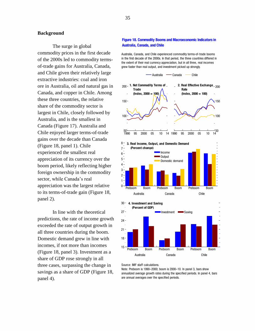
35

Background

The surge in global

commodity prices in the first decade

of the 2000s led to commodity terms-

of-trade gains for Australia, Canada,

and Chile given their relatively large

extractive industries: coal and iron

ore in Australia, oil and natural gas in

Canada, and copper in Chile. Among

these three countries, the relative

share of the commodity sector is

largest in Chile, closely followed by

Australia, and is the smallest in

Canada (Figure 17). Australia and

Chile enjoyed larger terms-of-trade

gains over the decade than Canada

(Figure 18, panel 1). Chile

experienced the smallest real

appreciation of its currency over the

boom period, likely reflecting higher

foreign ownership in the commodity

sector, while Canada’s real

appreciation was the largest relative

to its terms-of-trade gain (Figure 18,

panel 2).

In line with the theoretical

predictions, the rate of income growth

exceeded the rate of output growth in

all three countries during the boom.

Domestic demand grew in line with

incomes, if not more than incomes

(Figure 18, panel 3). Investment as a

share of GDP rose strongly in all

three cases, surpassing the change in

savings as a share of GDP (Figure 18,

panel 4).

0

1

2

3

4

5

6

7

8

Preboom Boom Preboom Boom Preboom Boom

50

100

150

200

1990 95 2000 05 10 14

1. Net Commodity Terms of

Trade

(Index, 2000 = 100)

Source: IMF staff calculations.

Note: Preboom is 1990–2000; boom is 2000–10. In panel 3, bars show

annualized average growth rates during the specified periods. In panel 4, bars

are annual averages over the specified periods.

Australia Canada Chile

Figure 18. Commodity Booms and Macroeconomic Indicators in

Australia, Canada, and Chile

50

100

150

200

1990 95 2000 05 10 14

2. Real Effective Exchange

Rate

(Index, 2000 = 100)

15

18

21

24

27

30

Preboom Boom Preboom Boom Preboom Boom

Australia Canada Chile

Australia Canada Chile

3. Real Income, Output, and Domestic Demand

(Percent change)

Income

Output

Domestic demand

Investment Saving

4. Investment and Saving

(Percent of GDP)

Australia, Canada, and Chile experienced commodity terms-of-trade booms

in the first decade of the 2000s. In that period, the three countries differed in

the extent of their real currency appreciation, but in all three, real incomes

grew faster than real output, and investment picked up strongly.

36

Did Capital and Labor Reallocate

toward the Commodities and

Nontradables Sectors?

In all three countries, there was a

clear pickup in the growth rates of both

capital and labor in the extractive sector

during the boom period (Figure 19, panels

1-6).32 Higher investment in the sector

accounted for the bulk of the increase in

economy-wide investment in Australia and

Chile (Figure 19, panel 7). But the broader

changes in investment and employment

growth across the commodities,

manufacturing, and nontradables sectors

did not always conform to theoretical

predictions. Contrary to those predictions:

In Australia the pace of capital

accumulation in manufacturing

picked up during the boom period,

reflecting in part strong demand

from export markets (mainly east

Asia), while it declined in the

nontradables sector.33 A number of

suggest that an important part of the

capital stock increase in

manufacturing was partly related to

the mining boom itself. For

example, Barnes and others (2013)

32 To analyze sectoral shifts arising from the

commodity boom, the economy is disaggregated

into three sectors: extractive industries (fuels

and mining), manufacturing, and nontradables.

Agriculture is omitted for simplicity—it

accounts for 2 to 4 percent of aggregate value

added in the three countries studied.

33 In the 2000s, manufacturing exports to east

Asia accounted for more than one-third of total

manufacturing exports in Australia, about 15

percent in Chile, and about 5 percent in Canada.

In Australia, Canada, and Chile, the 2000–10 commodity boom period

coincided with a clear increase in both capital and labor in the extractive

sector; in Australia and Chile, that sector accounted for the bulk of economy-

wide capital accumulation in the period. Labor and capital in the three

countries did not shift notably into the nontradables sector.

–4–2024681012

Ext. Manuf. Nontrad.–4–2

02468

1012

Ext. Manuf. Nontrad.

–4–2024681012

Ext. Manuf. Nontrad.–4–2

02468

1012

Ext. Manuf. Nontrad.

–4–2024681012

Ext. Manuf. Nontrad.

Figure 19. Growth of Capital and Labor by Sector: Boom versus

Preboom Periods

(Average annual percent change)

1. Australia, Capital Stock 2. Australia, Labor

–4–2

02468

1012

Ext. Manuf. Nontrad.

Ext. (preboom) Manuf. (preboom) Nontrad. (preboom)

Ext. (boom) Manuf. (boom) Nontrad. (boom)

3. Canada, Capital Stock 4. Canada, Labor

5. Chile, Capital Stock 6. Chile, Labor

–0.6

–0.3

0.0

0.3

0.6

0.9

1.2

Australia Canada Chile–0.6

–0.3

0.0

0.3

0.6

0.9

1.2

Australia Canada Chile

Sectoral Contributions to the Change in Growth

(Relative to the Preboom Period)1

Extractive Manufacturing Nontradables

7. Capital Stock 8. Labor

Sources: Hofman and others 2015; Latin America KLEMS; World KLEMS; and

IMF staff calculations.

Note: Preboom is 1990–2000; boom is 2000–10. The contributions of the

agriculture sector are small and not shown. Ext. = extractive; Manuf. =

manufacturing; Nontrad. = nontradables.1The change in the growth of capital and labor relative to the preboom period is

decomposed into sectoral contributions. A sector's contribution to the change

in growth is calculated as the annual growth of capital or labor multiplied by the

weight of that sector in the total capital and labor stock and averaged across

the 10-year period.

Growth of Capital and Labor

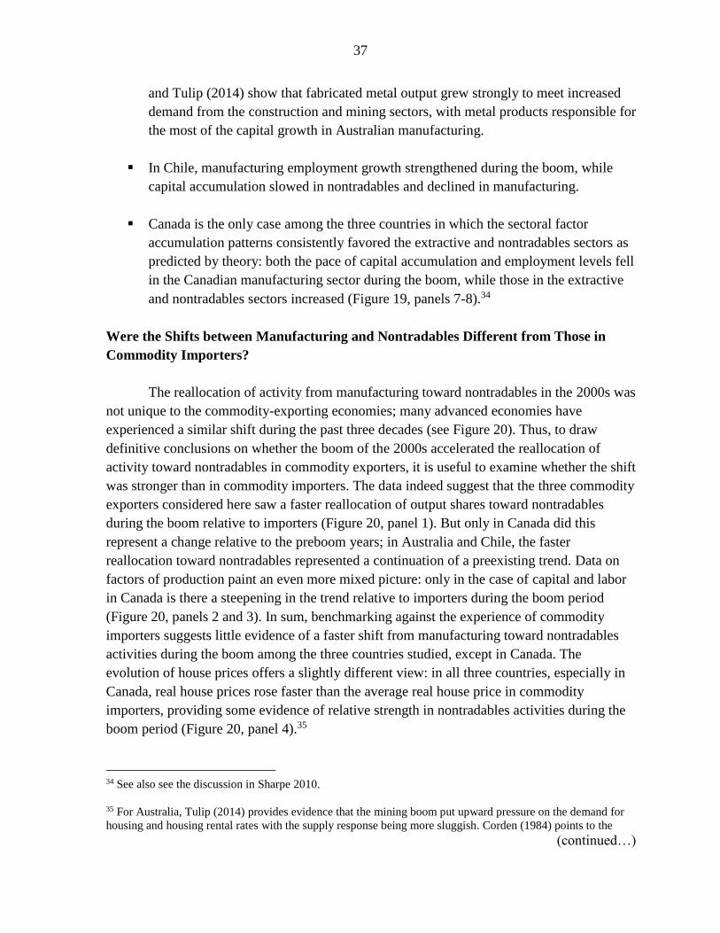
37

and Tulip (2014) show that fabricated metal output grew strongly to meet increased

demand from the construction and mining sectors, with metal products responsible for

the most of the capital growth in Australian manufacturing.

In Chile, manufacturing employment growth strengthened during the boom, while

capital accumulation slowed in nontradables and declined in manufacturing.

Canada is the only case among the three countries in which the sectoral factor

accumulation patterns consistently favored the extractive and nontradables sectors as

predicted by theory: both the pace of capital accumulation and employment levels fell

in the Canadian manufacturing sector during the boom, while those in the extractive

and nontradables sectors increased (Figure 19, panels 7-8).34

Were the Shifts between Manufacturing and Nontradables Different from Those in

Commodity Importers?

The reallocation of activity from manufacturing toward nontradables in the 2000s was

not unique to the commodity-exporting economies; many advanced economies have

experienced a similar shift during the past three decades (see Figure 20). Thus, to draw

definitive conclusions on whether the boom of the 2000s accelerated the reallocation of

activity toward nontradables in commodity exporters, it is useful to examine whether the shift

was stronger than in commodity importers. The data indeed suggest that the three commodity

exporters considered here saw a faster reallocation of output shares toward nontradables

during the boom relative to importers (Figure 20, panel 1). But only in Canada did this

represent a change relative to the preboom years; in Australia and Chile, the faster

reallocation toward nontradables represented a continuation of a preexisting trend. Data on

factors of production paint an even more mixed picture: only in the case of capital and labor

in Canada is there a steepening in the trend relative to importers during the boom period

(Figure 20, panels 2 and 3). In sum, benchmarking against the experience of commodity

importers suggests little evidence of a faster shift from manufacturing toward nontradables

activities during the boom among the three countries studied, except in Canada. The

evolution of house prices offers a slightly different view: in all three countries, especially in

Canada, real house prices rose faster than the average real house price in commodity

importers, providing some evidence of relative strength in nontradables activities during the

boom period (Figure 20, panel 4).35

34 See also see the discussion in Sharpe 2010.

35 For Australia, Tulip (2014) provides evidence that the mining boom put upward pressure on the demand for

housing and housing rental rates with the supply response being more sluggish. Corden (1984) points to the

(continued…)

38

The different patterns of sectoral reallocation across the three countries can be

attributed in part to the destination of their export manufacturing products. Among the

countries, Australia—which saw a pickup in manufacturing investment during the boom

period—sent a relatively larger share of its manufacturing exports to east Asia, particularly

China, on the eve of the boom. In contrast, the majority of Canada’s manufacturing exports

went to the United States, where manufacturing output growth slowed in the 2000s. To the

extent that booms in commodity prices coincide with strong global activity, Dutch disease

effects in commodity exporters could be offset, especially if the manufacturing sector has

trade linkages with faster-growing countries and regions.36

Did the Reallocation of Activity Hamper Aggregate TFP Growth?

The evidence on sectoral growth rates of output, capital, and labor points to

unambiguous shifts toward the commodity sector as well as shifts—though not as

consistent—toward nontradables activities. To examine whether these changes had an impact

on economy-wide TFP growth, the latter is decomposed into within-sector and between-

sector effects, applying the decomposition in Dabla-Norris and others 2015.

The decomposition is based on the following specification:

𝑡𝑓𝑝𝑡 −𝑡𝑓𝑝𝑡−1 =∑ ω𝑖,𝑡−1𝑖 (𝑡𝑓𝑝𝑖,𝑡 −𝑡𝑓𝑝𝑖,𝑡−1) +∑ 𝑡𝑓𝑝𝑖,𝑡𝑖 (ω𝑖,𝑡 −ω𝑖,𝑡−1),

in which 𝑖 refers to the sectors of the economy (here, extractive commodities,

manufacturing, and nontradables); 𝑡𝑓𝑝𝑡 and 𝑡𝑓𝑝𝑖,𝑡refer to economy-wide and sectoral TFP,

respectively; and ω𝑖,𝑡 is the share of real value added of sector 𝑖. The first term on the right

side is the within-sector effect given by the weighted sum of TFP growth in each sector. The

second term is the between-sector effect, which captures the effect of the sectoral reallocation

of real value added on aggregate TFP growth.

impact of immigration during commodity booms which places upward pressure on the demand for

nontradables.

36 See Box 2.1 in Chapter 2 of the October 2015 World Economic Outlook. Corden (1984) also shows that

immigration into economies experiencing large commodity booms can offset Dutch disease effects.

39

Data from Latin America

KLEMS and World KLEMS indicate

that aggregate TFP growth declined in

all three case study countries during the

commodity boom relative to the

previous decade and even turned

negative in Australia and Chile. The

decomposition indicates that this decline

was entirely due to the within-sector

effect (Figure 19, panels 1, 3, and 5).

The between-sector effect in fact

attenuated the decline in TFP,

particularly in Canada.37 This finding of

a negative contribution from the within-

sector effect holds more broadly for

Latin American economies (Aravena

and others 2014; Hofman and

others 2015).

Declining TFP growth in

extractive industries and manufacturing

appears to be a common factor behind

the weak within-sector TFP

performance in all three cases

(Figure 19, panels 2, 4, and 6). A

marked decline in TFP growth in

nontradables was also a key factor in

Australia and Chile, including due to

lower TFP growth in construction

towards the latter part of the boom

period. The weak TFP growth in the

extractive sectors during the boom is

likely to have been associated with the

time-to-build associated with large-scale

mining investments and the tapping of

less efficient mines in all three cases

37 See the discussion in Sharpe (2010) for details

on regional contributors to the positive

contributors to sectoral reallocation.

0.6

0.8

1.0

1.2

1.4

1990 93 96 99 2002 05 07

Figure 20. Evolution of Activity in Nontradables Relative to

Manufacturing, Commodity Exporters Relative to Commodity

Importers

1. Ratio of Nontradables Output to Manufacturing Output,

Relative to That of Commodity Importers

(Index, 2000 = 1)

Sources: Haver Analytics; Hofman and others 2015; Latin America KLEMS;

national authorities; World KLEMS; and IMF staff calculations.

Note: Panels 1–3 show the evolution in commodity exporters of the ratios of

output, capital, and labor in nontradables to those in manufacturing, scaled by

the average ratio across a sample of commodity importers in the same year. An

increase in the trend of a ratio beginning in 2000 relative to the pre-2000 trend

indicates that the reallocation from manufacturing to nontradables in

commodity exporters intensified relative to that in importers during the

commodity boom. Panel 4 shows the evolution of real house prices in

commodity exporters scaled by the average real house prices across commodity

importers. The sample of commodity importers comprises Denmark, Finland,

Germany, Japan, Sweden, the United Kingdom, and the United States.

Australia Canada Chile

0.6

0.8

1.0

1.2

1.4

1990 93 96 99 2002 05 07

2. Ratio of Nontradables Capital Stock to Manufacturing

Capital Stock, Relative to That of Commodity Importers

(Index, 2000 = 1)

0.6

0.8

1.0

1.2

1.4

1990 93 96 99 2002 05 07

0.6

0.8

1.0

1.2

1.4

1.6

1990 93 96 99 2002 05 08 11

3. Ratio of Nontradables Labor to Manufacturing Labor,

Relative to That of Commodity Importers

(Index, 2000 = 1)

4. Real House Prices, Relative to Those of Commodity Importers

(Index, 2004 = 1)

In Australia and Chile, the 2000–10 commodity boom did not accelerate the

shift of output, capital, and labor shares from manufacturing into

nontradables. House prices, however, grew more strongly in Australia,

Canada, and Chile than in their commodity-importing peers.

40

(Figure 20).38 The remoteness of extractive production sites may have contributed to higher

marginal costs in the supporting nontradables service industries.

In summary, the case studies point to substantial heterogeneity across countries in

terms of sectoral reallocation patterns during commodity booms. While all three countries

under study experienced a flow of factors of production into the commodity sector, they

experienced varying degrees of reallocation between the manufacturing and nontradables

sectors. The fact that the countries were exposed to different manufacturing export

destinations (that were experiencing different rates of expansion) seems to have been a factor

behind the varying intensity of sectoral reallocation; countries with stronger trading linkages

to faster-growing countries had more limited Dutch disease symptoms. Decompositions of

economy-wide TFP growth do not suggest that sectoral reallocation hindered TFP growth

during the commodity boom of the 2000s but instead point to a marked decline in

productivity growth within sectors. Understanding the mechanisms behind the drop in TFP

growth in these economies is an important area for future research.39

V. CONCLUSIONS

The evidence presented in this paper suggests that fluctuations in international

commodity prices, through their impact on domestic spending, can lead to sizable output

fluctuations in commodity exporters. In exporters of energy and metals, the comovement

between output and the commodity terms of trade tends to be particularly strong. It is also

stronger in countries with lower levels of financial development, more procyclical fiscal

policies, and less flexible exchange rates.

The strong investment response to changes in the commodity terms of trade means

that the latter affect not only actual output, but also potential output. As a result, the growth

of potential output can be expected to decline during downswings in commodity prices. The

change in the cyclical component of output is, however, about twice the size of the change in

potential output, the structural component.

Against the backdrop of the recent declines in the commodity prices, the findings of

the paper suggest that the growth slowdown in commodity exporters mirrors experiences

during earlier downswings. The slowdown could even be larger than those experienced in

past episodes, since the terms-of-trade upswings that many exporters experienced in the first

38 See the discussion in Francis 2008 and Sharpe 2010. This TFP weakness in extractive commodities comes in

stark contrast to the strong positive TFP growth of agricultural commodities in all three country cases,

particularly during the second half of the boom period.

39 Recent studies of this issue include Parham 2012 and Barnes and others 2013 for Australia and Sharpe 2010

and Baldwin and others 2014 for Canada.

41

decade of the 2000s were much larger than earlier ones. As a result, they may have led to

much larger increases in actual and potential output growth than in the past upswings

analyzed in the paper. If the terms-of-trade downswings are now also larger, the declines in

growth would likely be correspondingly larger as well.

The paper’s regression-based analysis indeed suggests that the recent commodity

price declines, together with the weak commodity price outlook, could subtract about 1

percentage point on average from the growth rate of commodity exporters in 2015–17

relative to 2012–14. For energy exporters, the reduction in growth could be even larger—

about 2¼ percentage points on average. The projected drag on the growth of potential output

is about 1/3 percentage point on average for commodity exporters and 2/3 percentage point

on average for energy exporters.

At the same time, many commodity exporters have moved toward policy frameworks

and structural characteristics that are more conducive to smoothing the macroeconomic

effects of terms-of-trade fluctuations—less procyclical fiscal policies, more flexible

exchange rates, and deeper financial systems. These changes could mitigate some of the

growth impact of commodity price downswings.

The analysis in the paper suggests that policymakers must avoid overestimating

output gaps and the scope for expansionary macroeconomic policies to support demand. As

commodity-exporting economies are likely to overheat toward the end of a prolonged surge

in commodity prices, the growth slowdown in the immediate aftermath of the boom most

likely reflects a cooling of output toward potential, which may itself be growing at a reduced

pace, given a slowdown in investment. If indicators of slack show few signs of output having

fallen below potential, expansionary monetary and fiscal policies are more likely to raise

inflation than to sustainably raise investment and employment.

In countries where output has fallen below potential, supportive domestic demand

policies could help avoid a costly underutilization of resources. But two considerations

suggest that the drop in the commodity terms of trade may itself limit the scope to ease

macroeconomic policies. First, in economies with some exchange rate flexibility, currency

depreciation may have led to an easing of monetary conditions without a change in the stance

of monetary policy; thus, any easing in the stance could risk further depreciation and

unwelcome increases in inflation. In other economies, declining resource-based fiscal

revenues may call for fiscal adjustment to secure debt sustainability.

Although the comovement of potential output with the commodity terms of trade

tends to be less pronounced than that of actual output, the analysis in this paper suggests that

declining growth of potential output exacerbates the post boom slowdowns. The decline in

42

the structural component of growth suggests that the policy agenda to restore stronger growth

in commodity exporters should include targeted structural reforms to alleviate the binding

supply-side bottlenecks and boost productivity growth.

43

REFERENCES

Adler, Gustavo, and Nicolás E. Magud. 2015. “Four Decades of Terms-of-Trade Booms: A

Metric of Income Windfall.” Journal of International Money and Finance 55: 162–92.

Albino-War, Maria A., Svetlana Cerovic, Francesco Grigoli, Juan Carlos Flores, Javier

Kapsoli, Haonan Qu, Yahia Said, Bahrom Shukurov, Martin Sommer, and SeokHyun

Yoon. 2014. “Making the Most of Public Investment in MENA and CCA Oil-

Exporting Countries.” IMF Staff Discussion Note 14/10, International Monetary

Fund, Washington.

Aravena, Claudio, Juan Fernández, André Hofman, and Matilde Mas. 2014. Structural

Change in Four Latin American Countries: An International Perspective.

Macroeconomics of Development Series No. 150. Santiago: Economic Commission

for Latin America and the Caribbean.

Arezki, Rabah, and Kareem Ismail. 2013. “Boom-Bust Cycle, Asymmetrical Fiscal Response

and the Dutch Disease.” Journal of Development Economics 101: 256–67.

Baldwin, John R., Wulong Gu, Ryan Macdonald, and Beiling Yan. 2014. “Productivity:

What Is It? How Is It Measured? What Has Canada’s Performance Been over the

Period 1961 to 2012?” Canadian Productivity Review 38.

Barnes, Paula., Leo Soames, Cindy Li, and Marcela Munoz, 2013, “Productivity in

Manufacturing: Measurement and Interpretation,” Productivity Commission Staff

Working Paper, November 2013.

Barro, Robert, and Jong-Wha Lee. 2010. “A New Data Set of Educational Attainment in the

World, 1950–2010.” Journal of Development Economics 104: 184–98.

Benigno, Gianluca, and Luca Fornaro. 2014. “The Financial Resource Curse.” Scandinavian

Journal of Economics 116 (1): 58–86.

Berg, Andrew, Edward F. Buffie, Catherine Pattillo, Rafael Portillo, Andrea Presbitero, and

Luis-Felipe Zanna. Forthcoming. “Some Misconceptions about Public Investment

Efficiency and Growth.” IMF Working Paper, International Monetary Fund,

Washington.

Berg, Andrew, Rafael Portillo, Shu-Chun S. Yang, and Luis-Felipe Zanna. 2013.

“Government Investment in Resource-Abundant Developing Countries.” IMF

Economic Review 61: 92–129.

44

Bjørnland, Hilde Christiane. 1998. “The Economic Effects of North Sea Oil on the

Manufacturing Sector.” Scottish Journal of Political Economy 45 (5): 553–85.

———, and Leif A. Thorsrud. Forthcoming. “Boom or Gloom? Examining the Dutch

Disease in Two-Speed Economies.” Economic Journal.

Blagrave, Patrick, Roberto Garcia-Saltos, Douglas Laxton, and Fan Zhang. 2015. “A Simple

Multivariate Filter for Estimating Potential Output.” IMF Working Paper 15/79,

International Monetary Fund, Washington.

Cashin, Paul, Luis Felipe Céspedes, and Ratna Sahay. 2004. “Commodity Currencies and the

Real Exchange Rate.” Journal of Development Economics 75 (1): 239–68.

Céspedes, Luis Felipe, and Andrés Velasco. 2012. “Macroeconomic Performance during

Commodity Price Booms and Busts.” IMF Economic Review 60 (4): 570–99.

Chen, Yu-chin, and Kenneth Rogoff. 2003. “Commodity Currencies.” Journal of

International Economics 60 (1): 133–60.

Collier, Paul, Rick van der Ploeg, Michael Spence, and Anthony J. Venables. 2010.

“Managing Resource Revenues in Developing Economies.” IMF Staff Papers 57 (1):

84–118.

Corden, Walter M. 1981. “The Exchange Rate, Monetary Policy and North Sea Oil: The

Economic Theory of the Squeeze on Tradeables.” Oxford Economic Papers 33: 23–

46.

———, 1984, “Booming Sector and Dutch Disease Economics: Survey and Consolidation”,

Oxford Economic Papers, New Series, Vol. 36, No. 3 (Nov., 1984), pp. 359-380.

———, and J. Peter Neary. 1982. “Booming Sector and De-industrialisation in a Small Open

Economy.” Economic Journal 92 (368): 825–48.

Dabla-Norris, Era, Si Guo, Vikram Haksar, Minsuk Kim, Kalpana Kochhar, Kevin Wiseman,

and Aleksandra Zdzienicka. 2015. “The New Normal: A Sector-Level Perspective on

Productivity Trends in Advanced Economies.” IMF Staff Discussion Note 15/03,

International Monetary Fund, Washington.

45

De Gregorio, José. 2015. “From Rapid Recovery to Slowdown: Why Recent Economic

Growth in Latin America Has Been Slow.” Policy Briefs PB15-6, Peterson Institute

for International Economics, Washington.

Deaton, Angus, and Ronald Miller. 1996. “International Commodity Prices, Macroeconomic

Performance and Politics in Sub-Saharan Africa.” Journal of African Economies 5

(3): 99–191.

Dehn, Jan. 2000. “The Effects on Growth of Commodity Price Uncertainty and Shocks.”

Policy Research Working Paper 2455, World Bank, Washington.

Eichengreen, Barry. 2008. “The Real Exchange Rate and Economic Growth.” Commission

on Growth and Development Working Paper 4, World Bank, Washington.

Ellman, M. 1981. “Natural Gas, Restructuring and Re-industrailisation: The Dutch

Experience of Industrial Policy”, in Barker , T. and Brailovsky, V. (eds), Oil or

Industry? London: Academic Press.

Enders, K. and Herberg, H. (1983), “The dutch Disease: Causes, Consequences, Cure and

Calmatives”, Welwirtschaftliches Archiv 119, 3, 473-97.

Erten, Bilge, and Jose Antonio Ocampo. 2012. “Super-cycles of Commodity Prices since the

Mid-Nineteenth Century.” DESA Working Paper No. 110, United Nations

Department of Economic and Social Affairs, New York.

Fornero, Jorge, Markus Kirchner, and Andrés Yany. 2014. “Terms of Trade Shocks and

Investment in Commodity Exporting Economies.” Paper presented at “Commodity

Prices and Macroeconomic Policy,” 18th Annual Conference of the Central Bank of

Chile, Santiago, October 23.

Foster, Vivien, and Cecilia Briceño-Garmendia, eds. 2010. Africa’s Infrastructure: A Time

for Transformation. Washington: Agence Française de Développement and World

Bank.

Francis, Michael. 2008. “Adjusting to the Commodity-Price Boom: The Experiences of Four

Industrialized Countries.” Bank of Canada Review (Autumn): 29–41.

Frankel, Jeffrey A. 2012. “The Natural Resource Curse: A Survey of Diagnoses and Some

Prescriptions.” In Commodity Price Volatility and Inclusive Growth in Low-Income

Countries, edited by Rabah Arezki, Catherine A. Patillo, Marc Quintyn, and Min Zhu.

Washington: International Monetary Fund.

46

Gelb, Alan, and Associates. 1988. Oil Windfalls: Blessing or Curse? New York: Oxford

University Press.

Gregory, R. G. (1976), “Some Implications of the Growth in the Mineral Sector”, Australian

Journal of Agricultural Economics 20 (August), 71-91.

Grigoli, Francesco, Alexander Herman, Andrew Swiston, and Gabriel Di Bella. 2015.

“Output Gap Uncertainty and Real-Time Monetary Policy.” IMF Working Paper

15/14, International Monetary Fund, Washington.

Gruss, Bertrand. 2014. “After the Boom—Commodity Prices and Economic Growth in Latin

America and the Caribbean.” IMF Working Paper 14/154, International Monetary

Fund, Washington.

Gupta, Pranav, Bin Grace Li, and Jiangyan Yu. 2015. “From Natural Resource Boom to

Sustainable Economic Growth: Lessons for Mongolia.” IMF Working Paper 15/90,

International Monetary Fund, Washington.

Gupta, Sanjeev, Alvar Kangur, Chris Papageorgiou, and Abdoul Wane. 2014. “Efficiency-

Adjusted Public Capital and Growth.” World Development 57: 164–78.

Gylfason, Thorvaldur. 2001. “Natural Resources, Education and Economic Development.”

European Economic Review 45 (4–6): 847–59.

Harding, Don, and Adrian Pagan. 2002. “Dissecting the Cycle: A Methodological

Investigation.” Journal of Monetary Economics 49 (2): 365–81.

Harding, Torfinn, and Anthony J. Venables. 2013. “The Implications of Natural Resource

Exports for Non-resource Trade.” OxCarre Research Paper 103, Department of

Economics, Oxford Centre for the Analysis of Resource Rich Economies, Oxford,

United Kingdom.

Hofman, André, Matilde Mas, Claudio Aravena, and Juan Fernandez de Guevara. 2015. “LA

KLEMS: Economic Growth and Productivity in Latin America.” In The World

Economy: Growth or Stagnation? edited by Dale W. Jorgenson, Kyoji Fukao, and

Marcel P. Timmer. Cambridge: Cambridge University Press.

47

Husain, Aasim M., Kamilya Tazhibayeva, and Anna TerMartirosyan. 2008. “Fiscal Policy

and Economic Cycles in Oil-Exporting Countries.” IMF Working Paper 08/253,

International Monetary Fund, Washington.

International Monetary Fund (IMF). 2006. “Methodology for CGER Exchange Rate

Assessments.” Unpublished, Washington.

———. 2012. “Macroeconomic Policy Frameworks for Resource-Rich Developing

Countries.” Washington. https:// www.imf.org/external/np/pp/eng/2012/082412.pdf.

———. 2015. “Making Public Investment More Efficient.” Staff Report, Washington.

Ismail, Kareem. 2010. “The Structural Manifestation of the ‘Dutch Disease’: The Case of Oil

Exporting Countries.” IMF Working Paper 10/103, International Monetary Fund,

Washington.

Jordà, Òscar. 2005. “Estimation and Inference of Impulse Responses by Local Projections.”

American Economic Review 95 (1): 161–82.

Kalemli-Özcan, Şebnem, Harl E. Ryder, and David N. Weil. 2000. “Mortality Decline,

Human Capital Investment, and Economic Growth.” Journal of Development

Economics 62 (1): 1–23.

Kilian, Lutz. 2009. “Not All Oil Price Shocks Are Alike: Disentangling Demand and Supply

Shocks in the Crude Oil Market.” American Economic Review 99 (3): 1053–69.

Kohli, Ulrich. 2004. “Real GDP, Real Domestic Income, and Terms-of-Trade Changes.”

Journal of International Economics 62 (1): 83–106.

Krugman, Paul. 1987. “The Narrow Moving Band, the Dutch Disease, and the Competitive

Consequences of Mrs. Thatcher: Notes on Trade in the Presence of Dynamic Scale

Economies.” Journal of Development Economics 27 (1–2): 41–55.

Lalonde, René, and Dirk Muir. 2007. “The Bank of Canada’s Version of the Global

Economy Model (BoC-GEM).” Bank of Canada Technical Report 98, Bank of

Canada, Ottawa.

Lane, Philip R., and Gian Maria Milesi-Ferretti. 2007. “The External Wealth of Nations

Mark II: Revised and Extended Estimates of Foreign Assets and Liabilities, 1970–

2004.” Journal of International Economics 73 (2): 223–50.

48

Magud, Nicolás, and Sebastián Sosa. 2013. “When and Why Worry about Real Exchange

Rate Appreciation? The Missing Link between Dutch Disease and Growth.” Journal

of International Commerce, Economics, and Politics 4 (2): 1–27.

Matsuyama, Kiminori. 1992. “Agricultural Productivity, Comparative Advantage, and

Economic Growth.” Journal of Economic Theory 58 (2): 317–34.

McKinnon, R. I. (1976), “International Transfers and Non-traded Commodities: The

Adjustment Problem”, in Leipziger, D. M. (eds), The International Monetary System

and the Developing Nations, Washington DC: Agency for International Development.

McMahon, Gary, and Susana Moreira. 2014. “The Contribution of the Mining Sector to

Socioeconomic and Human Development.” Extractive Industries for Development

Series 30, World Bank, Washington.

Melina, Giovanni, Shu-Chun S. Yang, and Luis-Felipe Zanna. 2014. “Debt Sustainability,

Public Investment, and Natural Resources in Developing Countries: The DIGNAR

Model.” IMF Working Paper 14/50, International Monetary Fund, Washington.

Mendoza, Enrique G. 1995. “The Terms of Trade, the Real Exchange Rate, and Economic

Fluctuations.” International Economic Review 36 (1): 101–37.

Oster, Emily, Ira Shoulson, and E. Ray Dorsey. 2013. “Limited Life Expectancy, Human

Capital and Health Investments.” American Economic Review 103 (5): 1977–2002.

Parham, Dean. 2012. “Australia’s Productivity Growth Slump: Signs of Crisis, Adjustment

or Both?” Visiting Researcher Paper, Australian Government, Productivity

Commission, Melbourne.

Pesenti, Paolo. 2008. “The Global Economy Model: Theoretical Framework.” IMF Staff

Papers 55 (2): 243–84.

Reinhart, Carmen M., and Kenneth S. Rogoff. 2004. “The Modern History of Exchange Rate

Arrangements: A Reinterpretation.” Quarterly Journal of Economics 119 (1): 1–48.

Roache, Shaun K. 2012. “China’s Impact on World Commodity Markets.” IMF Working

Paper 12/115, International Monetary Fund, Washington.

Rodrik, Dani. 2008. “The Real Exchange Rate and Economic Growth.” Brookings Papers on

Economic Activity 39 (2): 365–439.

49

———. 2015. “Premature Deindustrialization.” NBER Working Paper 20935, National

Bureau of Economic Research, Cambridge, Massachusetts.

Rosenbaum, Paul R., and Donald B. Rubin. 1983. “The Central Role of the Propensity Score

in Observational Studies for Causal Effects” Biometrika 70 (1): 41–55.

Sala-i-Martin, Xavier, and Arvind Subramanian. 2003. “Addressing the Natural Resource

Curse: An Illustration from Nigeria.” IMF Working Paper 03/139, International

Monetary Fund, Washington.

Schmitt-Grohé, Stephanie, and Martín Uribe. 2015. “How Important Are Terms of Trade

Shocks?” NBER Working Paper 21253, National Bureau of Economic Research,

Cambridge, Massachusetts.

Sharpe, Andrew, 2010, “Unbundling Canada’s Weak Productivity Performance: The Way

Forward”, Centre for the Study of Living Standards.

Snape, R. H., (1977), “Effects of Mineral Development on the Economy”, Australian Journal

of Agricultural Economics 21 (December), 147-56.

Spatafora, Nikola, and Irina Tytell. 2009. “Commodity Terms of Trade: The History of

Booms and Busts.” IMF Working Paper 09/205, International Monetary Fund,

Washington.

Spatafora, Nikola, and Andrew Warner. 1995. “Macroeconomic Effects of Terms-of-Trade

Shocks.” Policy Research Working Paper 1410, World Bank, Washington.

Steenkamp, Daan. 2014. “Structural Adjustment in New Zealand since the Commodity

Boom.” Reserve Bank of New Zealand Analytical Note AN 2014/2, Reserve Bank of

New Zealand, Wellington.

Teulings, Coen N., and Nikolay Zubanov. 2014. “Is Economic Recovery a Myth? Robust

Estimation of Impulse Responses.” Journal of Applied Econometrics 29 (3): 497–514.

Tulip, Peter, 2014, “The Effect of the Mining Boom on the Australian Economy”, Reserve

Bank of Australia, December Quaterly Bulletin.

van der Ploeg, Frederick. 2011. “Natural Resources: Curse or Blessing?” Journal of

Economic Literature 49 (2): 366–420.

50

van Wijnbergen, Sweder J. G. 1984a. “The ‘Dutch Disease’: A Disease after All?” Economic

Journal 94 (373): 41–55.

———. 1984b. “Inflation, Employment, and the Dutch Disease in Oil-Exporting Countries:

A Short-Run Disequilibrium Analysis.” Quarterly Journal of Economics 99 (2): 233–

50.

Warner, Andrew M. 2014. “Public Investment as an Engine of Growth.” IMF Working Paper

14/148, International Monetary Fund, Washington.