TRACKING A SYSTEM OF SHARED AUTONOMOUS VEHICLES ACROSS THE 1

AUSTIN, TEXAS NETWORK USING AGENT-BASED SIMULATION 2 3

Jun Liu, Ph.D. 4 Postdoctoral Fellow 5

Center for Transportation Research 6 The University of Texas at Austin – UTA 4.228 7

jun.liu@utexas.edu 8 9

Kara M. Kockelman, Ph.D., P.E. 10 (Corresponding Author) 11

Professor, and E.P. Schoch Professor in Engineering 12 Department of Civil, Architectural and Environmental Engineering 13

The University of Texas at Austin – 6.9 E. Cockrell Jr. Hall 14 Austin, TX 78712-1076 15

kkockelm@mail.utexas.edu 16 Phone: 512-471-0210 & FAX: 512-475-8744 17

18 Patrick M. Boesch 19 Research Assistant 20 IVT, ETH Zurich 21

CH-8093 Zurich, Switzerland 22 patrick.boesch@ivt.baug.ethz.ch 23

24 Francesco Ciari, Ph.D. 25

Research Associate 26 IVT, ETH Zurich 27

CH-8093 Zurich, Switzerland 28 ciari@ivt.baug.ethz.ch 29

30

Under review for publication in Transportation, March 2016 31

32

ABSTRACT 33

This study provides a large-scale micro-simulation of transportation patterns in a metropolitan 34

area when relying on a system of shared autonomous vehicles (SAVs). The six-county region of 35

Austin, Texas is used for its land development patterns, demographics, networks, and trip tables. 36

The agent-based MATSim toolkit allows modelers to track individual travelers and individual 37

vehicles, with great temporal and spatial detail. MATSim’s algorithms help improve individual 38

travel plans (by changing tour and trip start times, destinations, modes, and routes). Here, the 39

SAV mode requests were simulated through a stochastic process for four possible fare levels: 40

$0.50, $0.75, $1, and $1.25 per trip-mile. These fares resulted in mode splits of 50.9%, 12.9 %, 41

10.5%, and 9.2% of the region’s person-trips, respectively. 42

Mode choice results show longer-distance travelers preferring SAVs to private, human-driven 43

vehicles (HVs) - thanks to the reduced burden of SAV travel (since one does not have to drive 44

the vehicle). For travelers whose households do not own an HV, SAVs (rather than transit, 45

walking and biking) appear preferable for trips under 10 miles, which is the majority of those 46

travelers’ trip-making. It may be difficult for traditional transit services and operators to survive 1

once SAVs become available in regions like Austin, where dedicated rail lines and bus lanes are 2

few. Simulation of SAV fleet operations suggest that higher fare rates allow for greater vehicle 3

replacement (ranging from 5.6 to 7.7 HVs per SAV, assuming that the average SAV serves 17 to 4

20 person-trips per day); this is due to travel demands shifting away from longer trip distances, 5

when fares rise. Empty vehicle miles traveled by the fleet of SAVs ranged from 7.8 percent to 6

14.2 percent, across the scenarios in this study. Implications of mobility and sustainability 7

benefits of SAVs are also discussed in the paper. 8

KEYWORDS 9

Shared Autonomous Vehicles, Car-sharing, Agent-Based Simulation, Mode Choice, Travel 10

Demand Modeling 11

INTRODUCTION 12

Autonomous vehicles (AVs) may begin to transform surface transportation systems in the next 13

few years. Human-controlled vehicles (HVs) are normally owned by the traveler, and are parked 14

95% of the time (Barter, 2013). Since AVs can self-drive (to find a parking space and refuel), 15

there is much less need for private vehicle ownership. Shared AVs (SAVs) are expected to 16

become a major travel mode, bringing expensive transport technologies to the masses well before 17

individuals may be able to afford their own AV (Kornhauser et al., 2013; Fagnant and 18

Kockelman, 2014a; Fagnant and Kockelman, 2015; Google, 2016; Uber, 2016). 19

Car-sharing allows many travelers to quickly access a fleet of automobiles without ownership 20

costs and responsibilities. Car-sharing is especially popular among younger travelers (Gagnier, 21

2013), making it a strong candidate for future mode choices. About 5.8 million people, around 22

the world, are already using car-sharing services, and users are anticipated to number 15 million 23

by 2020 (Tomlinson, 2016). SAVs improve car-sharing access times, by bringing empty vehicles 24

directly to the user (avoiding search costs) and dropping off passengers at their requested 25

destinations, without worrying about parking (or, presumably, refueling). SAV use in travel-rich 26

environments is likely to bring economies of scale and density, with little empty travel, out-27

performing many other modes (Chen et al. 2016). 28

AV use is expected to reduce crash counts and crash severities (Kockelman and Li, 2016), travel 29

costs (in terms of travel time burdens for those who previously were at the wheel, maneuvering 30

their vehicles through traffic, rain, and darkness), while facilitating longer-distance trip-making 31

and travel by those with disabilities or those without licenses (Anderson et al., 2014; Fagnant and 32

Kockelman, 2014a; Chen and Kockelman, 2015; Fagnant and Kockelman, 2015; Chen et al., 33

2016). If VMT and vehicle sizes do not increase much, AV technologies may also reduce energy 34

consumption and emissions (Paul et al., 2011; Folsom, 2012; Ford, 2012; Chapin et al., 2013; 35

Bansal et al., 2015; Liu et al., 2015; Liu and Kockelman, 2016; Reiter and Kockelman, 2016) 36

Leob et al., 2016). 37

This study offers insights into the operations of a system of SAVs the Capital Area Metropolitan 38

Planning Organization (CAMPO) region of Texas, with the city of Austin at its core. A large-39

scale micro-simulation was constructed to mimic daily travel tours by individuals across the 2.3 1

million person (895 thousand household) region. Using CAMPO’s (2015) travel demand model 2

results across 2,102 traffic analysis zones (TAZs), an agent-based, large-scale transport 3

simulation platform called MATSim was employed (MATSim, 2016b). MATsim has been 4

applied by many researchers outside the U.S., including Horni et al. (2009) in their investigations 5

of shopping and leisure activities, Maciejewski and Nagel’s (2013) simulation of taxi services 6

around the Polish city of Mielec, Novose et al.’s (2015) exploration of transport’s energy 7

demands, and Ciari et al.’s (2016) car-sharing simulations for Zurich. 8

Travel patterns in MATSim are specified at the most disaggregate, individual level, with 9

persons’ daily activity plans serving as core model inputs. SAV mode choice is determined 10

through a random process, comparing deterministic utility scores of SAVs versus HVs versus 11

transit and other mode options. Research questions addressed here include: Who tends to prefer 12

SAVs and why?, How do SAVs serve requests and how many SAVs are needed in different 13

scenarios, to avoid long wait times?, and What are the mobility and other impacts of using 14

SAVs? The work seeks to provide insights for private and public sector stakeholders who hope 15

to implement SAVs systems. The results also provide guideposts to transportation planners and 16

policy (and decision-) makers who must plan for arrivals of these new technologies and modes. 17

METHODOLOGY 18

The work involved here can be described as a series of three major parts: 1) traveler activity 19

generation, 2) activity-based agent-based simulation, and 3) post–processing of outputs, as 20

shown in Figure 1. 21

22

Figure 1: Overview of research methodology 23

Reconstructing Travel Activity 24

This study used CAMPO’s (2015) existing, inter-TAZ travel demand (trip-count) predictions for 25

year 2020. OpenStreetMap (OSM) files were extracted to provide locations of homes and 26

businesses, and all road links and nodes, at much greater detail than MPOs tend to code their 27

roadway systems. The result of this intensive effort was a spatially detailed plan for each 28

traveler’s activities, chained or sequenced over time and space. Figure 2(a) shows CAMPO’s 6 1

counties and 2102 TAZs, expected to contain 2.33 million people and 895-thousand households 2

in year 2020 (CAMPO 2015); Figure 2(b) shows the road networks, including 30,460 directed 3

(one-direction) lane-miles, across 147,049 nodes and 234,444 links. The central areas, with 4

dense roadways, is the City of Austin. Note, the road network in a traditional four-step models of 5

CAMPO only contains 18,571 lane miles (CAMPO 2015); therefore, the network created in this 6

study has greater details. 7

8

Figure 2: Study region and road networks 9

Figure 3(a) shows the spatial distributions of population in CAMPO area, indicating the possible 10

trip start locations. According to the U.S.’s 2009 National Household Travel Survey (NHTS), the 11

average Texan makes 3.76 person-trips a weekday (versus 3.78 trips/day for the average 12

American). In total, about 8.8 million person-trips were constructed for this region. Then, these 13

simple trips were chained for individual travelers, to create a daily tour for performing planned 14

activities. The trip start location (or activity location) information came from building footprint 15

(and centroid) data were extracted from the OSM maps, as shown in Figure 3(b). 16

1

Figure 3: Generating a synthetic micro-population 2

Activity-based Agent-based Simulation 3

Transportation resources, e.g., road link capacity, are limited. People may have to modify their 4

(original) travel plans by adjusting trip start time, altering travel mode and route choices, or even 5

changing the destination choices (e.g., going somewhere else or cancelling a trip if possible), to 6

make the travel plans more executable and avoid the unacceptable loss of utility that is related to 7

the value of time, travel cost and the value of performing an activity. To obtain more realistic 8

and executable travel plans under transport constraints, this study employed MATSim, a large-9

scale agent-based transport simulation package, to model the each persons’ activities in a real-10

world regional transportation network (i.e., CAMPO region) and to observe on an individual 11

level how agents (representing travelers and vehicles) run in the network. In MATSim, all agents 12

try to maximize their utility in a co-evolutionary process until a dynamic user equilibrium (DUE) 13

is reached, i.e., no agent can further improve their mobility behavior by modifying their plans 14

(Bösch et al., 2016; Ciari et al., 2016). Unlike studies or programs where the utility is calculated 15

for travel only (the mode or route choice), the utility function in MATSim accounts for both the 16

travel and the activities: 17

18

∑

∑

(1)

19

where, = Total utility of a travel solution composed of a daily trip chain; = Utility of 1

travel for ith trip in a day; i = 1, 2, 3, …, q trips; = Travel time for ith trip; = 2

Utility of performing the jth activity in a day; j = 1, 2, 3, …, q+1 activities; and 3

= Duration of jth activity. The travel solution optimization is to maximize the total utility 4

of a chain of trips an agent may take to perform his or her planned activities. More details about 5 the MATSim scoring function are available in MATSim Book (MATSim, 2016b). 6 7

SAV Operations Simulation 8

Agents request the SAV service based on their travel plans. SAVs are initially distributed 9

according to the first group of travel requests in the early morning. In SAV operation 10

simulations, except the first group of requests, a travel request is assigned to the closest, 11

available SAV within a predefined service radius (SAV travel time to the start location of the 12

request). The assigned SAV moves to the start location of the travel request. The assigned SAV 13

can arrive before the end of the prior activity. In this case, the assigned SAV waits for the 14

traveler to finish the activity. If the traveler finishes the activity earlier than the SAV’s arrival, 15

the traveler waits for the SAV (the waiting time threshold is the predefined service radius of 16

SAVs). Once the SAV and the traveler are both ready, they move together to the trip end 17

location. After they arrive, the AV becomes available for a next request. Bösch et al. (2016) 18

showed more details about the SAV operation simulation package in their study (Bösch et al., 19

2016). 20

Implementing the Simulations 21

SAV travel demand was drawn based on the DUE travel plans, presuming that SAVs have the 22

same driving characters as HVs (e.g., the similar headway, travel speed, and vehicle size). It is 23

expected that not all travelers would choose SAVs and some drivers will remain using private 24

owned HVs (or even private AVs), or existing public transit. Mode choice between SAVs and 25

HVs (or transit) was conducted separately for households who own a HV and those who do not. 26

For households with at least one HV, their members have three options of travel modes (HV, 27

transit and SAV), and for those without a HV, there are only two options (transit and SAV). The 28

travel mode was stochastically determined based on discrete choice models (Chen and 29

Kockelman, 2015). 30

For travelers with privately owned HVs, the probability of using a SAV can be estimated to be: 31

(2)

32

where, = Deterministic utility of using a SAV; = Deterministic utility of using a HV; 33

and = Deterministic utility of using transit. For travelers without access to privately owned 34 HVs, the probability of using a SAV can be estimated to be: 35 36

(3)

The out-of-pocket cost and the value of time (of both in-vehicle and out-of-vehicle) were 1

considered when determining the utility: 2

1) Out-of-Pocket Cost. According to AAA, the average cost to own and operate a vehicle is 58 3

cents per mile (AAA, 2015). The cost of using a HV was assumed to be 60 cents per mile in 4

this study. For those who do not have access to a HV, the cost of using transit is important in 5

mode choice. The cost of taking transit in CMAPO area is somehow fixed based on the lines 6

and riding services, not based on the trip distance (Metro, 2016). According to the current 7

fare rates of Austin Public Transit, $2 per ride was assumed for the simulation 8

implementation. For SAVs, distance-based fare rates plus fixed costs were assumed in this 9

study. The fare rates in this study are the unit cost (per mile) of using a SAV, which can be 10

around or even higher than the cost of operating and owning a HV, because travelers do not 11

own SAVs. Four possible distance-based fare rates are assumed: $0.50, $0.75, $1 and $1.25 12

per mile. The fixed costs include membership fees and other additive charges (e.g., 13

insurance) which are unrelated to the service distance. For each SAV service, $1 fixed cost is 14

assumed. 15

16

2) Value of Time (VOT). According to the Urban Mobility Report by Texas Transportation 17

Institute (Schrank et al., 2015), the value of in-vehicle travel time (IVTT) for HV travelers is 18

estimated at $17.67 per hour. Similar to PT’s VOT, SAVs’ VOT is expected to be less than 19

that HVs’, because travelers (mainly the driver) will perceive the reduced burden of travel 20

due to no longer needing to drive and being able to perform other activities (such as reading, 21

working and resting). In this study, the value of IVTT for SAV and transit travelers is 22

assumed to be half of HVs’ associated VOT, $8.84 per hour. However, taking a bus may 23

result in longer IVTT because of the frequent stops. This study assumed that transit trips take 24

averagely 1.5 longer time to reach the destination than driving a HV, all other factors equal. 25

SAVs are expected to take the same IVTT as a HV would. Regarding the value of out-of-26

vehicle time (OVTT), a report by National Cooperative Highway Research Program 27

(NCHRP) provided an estimate of 2 to 3 times of the IVTT (NCHRP, 2012). Therefore, the 28

value of OVTT was assumed to be twice of IVTT, $35.34 per hour. 29

So, the utility function for using a HV is: 30

(4)

The utility function for using transit services is: 31

(5)

The utility function of SAVs is: 32

(6)

where, the travel distance and driving-based IVTT were obtained through the MATSim DUE 33

travel plans and the . and for transit services 34

was simulated in this study, randomly determined (between 0 to 15 minutes) based on the public 1

transit plans in Austin area (Metro, 2010). 2

The for SAVs is related to the dynamic distributions of available SAVs (Fagnant 3

and Kockelman. 2015). A random OVTT (ranging from 0 to 10 minutes and following a gamma 4

distribution with the shape parameter k = 2 and the scale parameter θ = 1) was made for a 5

traveler when a travel request is about to be made, to mimic a traveler roughly estimating his or 6

her waiting time when perfect information is not available. Note that, in the future, the SAV 7

services through information technologies (such as smartphone applications) are expected to 8

provide such real-time waiting time for each request, given certain SAV fleet size and the 9

operation schemes. Known the fare rate, travel distance, IVTT and OVTT, the probability of a 10

traveler choosing SAV for travel can be obtained. Then the decision of choosing either SAV, 11

transit or HV was made through a stochastic process. 12

With the travel mode determined, the travel demand for SAVs was pulled into the add-on SAV 13

operation simulations. The outputs of these simulations included the optimal SAV fleet size, 14

average waiting time, and many other perspectives of the SAV operations in CAMPO region, 15

given a certain fare rate. 16

SIMULATION RESULTS 17

Mode Choice for SAVs 18

As shown in Equations (2) through (6), the probability of a traveler choosing to use a SAV 19

depends on the travel distance, trip duration and waiting time, give a certain fare rate. This study 20

examined four possible fare rates ($0.50, $0.75, $1 and $1.25 per mile), resulting in four mode-21

split scenarios. Figure 4(a) shows the average probability of choosing a SAV over HV or transit 22

under four assumed fare rates and fixed cost $1 (relationships between travel distances). When 23

SAV fare rate is $0.5 per mile, the probability of choosing a SAV increases with the trip length 24

between 0 and 20 miles. When trip length reaches 20 miles, the probability is about 70%, and 25

after that the probability decreases as the length increases. At a lower fare rate, SAVs may be 26

more likely to be chosen than HVs while the travel distance increases, because of the reduced 27

burden of in-vehicle activities in SAVs. However, with the increase of trip length, SAVs may 28

lose their attractiveness because of the cost, compared with transit services (as transit is also with 29

reduced burden in-vehicle activities). In general, transit services may be not competitive for short 30

trips (owing to the walking and waiting time), but for long travels, such walking and waiting 31

time may become a small portion of the total duration of travel. That is why Figure 4(a) shows 32

when SAV fare rate is $0.5 per mile the probability of choosing SAV increases first (before 20 33

miles) and then deceases as the travel distance increases, because travelers prefer to choose a 34

cheaper travel mode (i.e., transit). When SAV fare rates are $0.75 per mile, the probability of 35

choosing a SAV increases with trip distance, until it reaches 10 miles. When fare rates are $1 and 36

$1.25 per mile are assumed, this probability is very small and falls with travel distance. When 37

SAV fare rates are high, long-distance travelers find SAVs to be too costly, so HV or transit 38

modes are chosen. 39

Figure 4(b) shows the shows the average probability of choosing a SAV over transit (for 1

travelers who do not have access to a HV). For four SAV fare rates, similar trends are found: as 2

the trip distance increases, the probability of choosing a SAV decreases. Noticeably, for trips 3

under 10 miles (which accounts for about 80% of all person-trips across the CAMPO region), 4

SAVs (under four possible fare rates) are expected to replace the transit services for most 5

travelers who do not have a privately owned vehicle. 6

Figure 4(c) summarizes the probabilities of choosing a SAV for two groups of travelers (with or 7

without access to a HV). Since about 85% of households own at least one HV, the totaled 8

probabilities are generally similar to what is shown in Figure 4(a) with slightly shifting up. After 9

obtaining the probability of choosing a SAV for travel, given the fare rate, travel distance, IVTT 10

and OVTT, a stochastic process was undertook to determine a travel model for each trip. 11

12

Figure 4: Probability of choosing SAV under four SAV fare rates assumptions, across 13

different trip distances 14

SAV Operations 15

SAVs were simulated to serve the MATSim DUE travel demand under four different fare rates, 16

$0.50, resulting in four levels of demand for SAVs: 17

1) 50.9% of trips request SAVs when fares are $0.50 per mile; 18

2) 12.9 % of trips request SAVs when fares are $0.75 per mile; 19

3) 10.5% of trips request SAVs when fares are $1 per mile; and 20

4) 9.2% of trips request SAVs when fares are $1.25 per mile. 1

To get the optimized SAV fleet size, an objective of SAV operations was made based on Bösch 2

et al. (Bösch et al., 2016). This objective was to meet about 95% of travel demand for SAVs 3

within two possible OVTT values: 1) on-time service if OVTT < 5 minutes, and 2) late service if 4

OVTT > 5 minutes but < 10 minutes. Note that, in real practice, the rest 5% of SAV travel 5

demand may still be able to be served if the users agree to wait for a SAV longer than 10 6

minutes, or they fall back to other travel modes, e.g., transit. 7

Figure 5(a) presents the simulation results (over all random seeds) from four scenarios (four fare 8

rates with fixed cost $1), regarding the SAV fleet size in percentage of travelers requesting 9

SAVs. The results include the shares of SAV service type: on-time service, late service and 10

unserved requests (waiting time > 10 minutes). Figure 5(b) shows the total shares of served 11

SAV requests including both on-time and late services along with the SAV fleet sizes. The SAV 12

service performances are generally consistent in four scenarios: with the increase in SAV fleet 13

size, more SAV requests can be served (Bösch et al., 2016). Table 1 summarizes the 14

performance of SAV systems serving 95% of SAV requests under four fare rates. 15

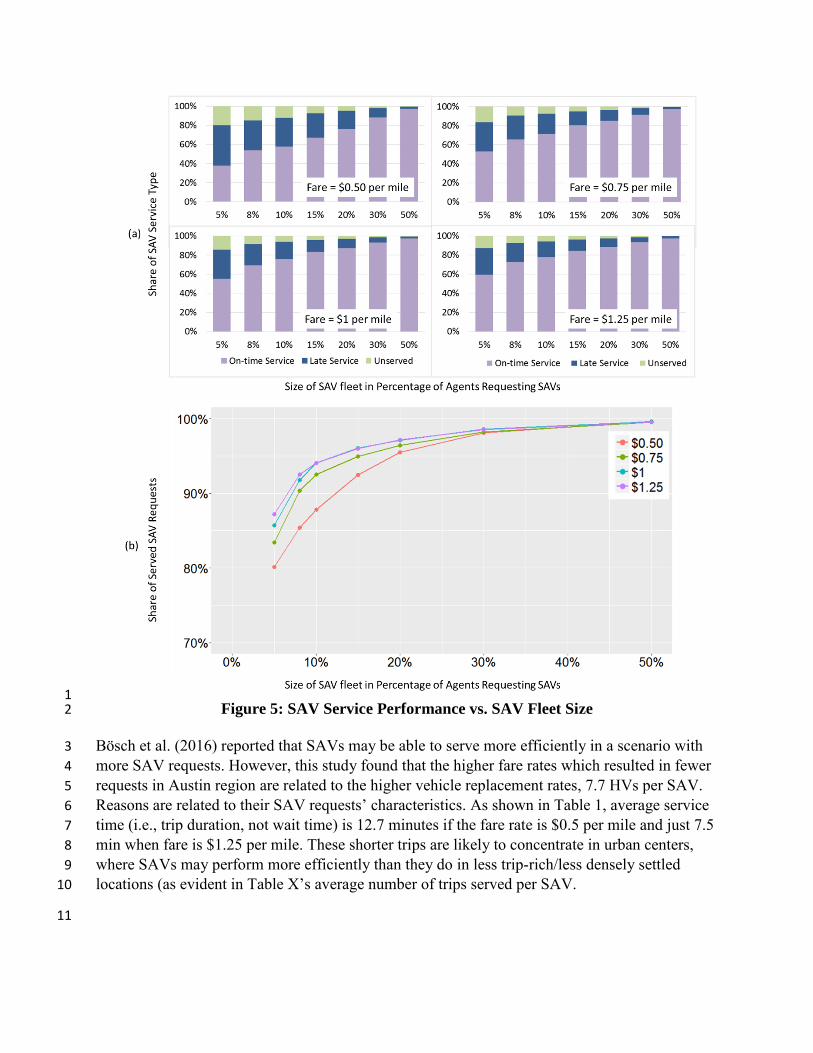
1 Figure 5: SAV Service Performance vs. SAV Fleet Size 2

Bösch et al. (2016) reported that SAVs may be able to serve more efficiently in a scenario with 3

more SAV requests. However, this study found that the higher fare rates which resulted in fewer 4

requests in Austin region are related to the higher vehicle replacement rates, 7.7 HVs per SAV. 5

Reasons are related to their SAV requests’ characteristics. As shown in Table 1, average service 6

time (i.e., trip duration, not wait time) is 12.7 minutes if the fare rate is $0.5 per mile and just 7.5 7

min when fare is $1.25 per mile. These shorter trips are likely to concentrate in urban centers, 8

where SAVs may perform more efficiently than they do in less trip-rich/less densely settled 9

locations (as evident in Table X’s average number of trips served per SAV. 10

11

Table 1: Performance of SAV system under four fare rates 1

Metric $0.5 $0.75 $1 $1.25

SAV demand in % of total trips 50.9% 12.9% 10.5% 9.2%

SAV fleet size in % of travelers 18% 15% 13% 13%

HV replacement rate 5.6 6.7 7.7 7.7

Average number of trips served per SAV 18.0 17.1 20.1 19.0

Extra VMT 7.8% 12.1% 14.2% 14.2%

Average waiting time (minute) 3.1 3.2 3.1 3.2

Average service time (minute) 12.7 8.9 7.9 7.5

% on-time service (waiting < 5 minutes) 72.6% 80.1% 81.1% 82.6%

% late service (waiting 5 to 10 minutes) 21.9% 14.8% 14.4% 12.9%

DISCUSSION 2

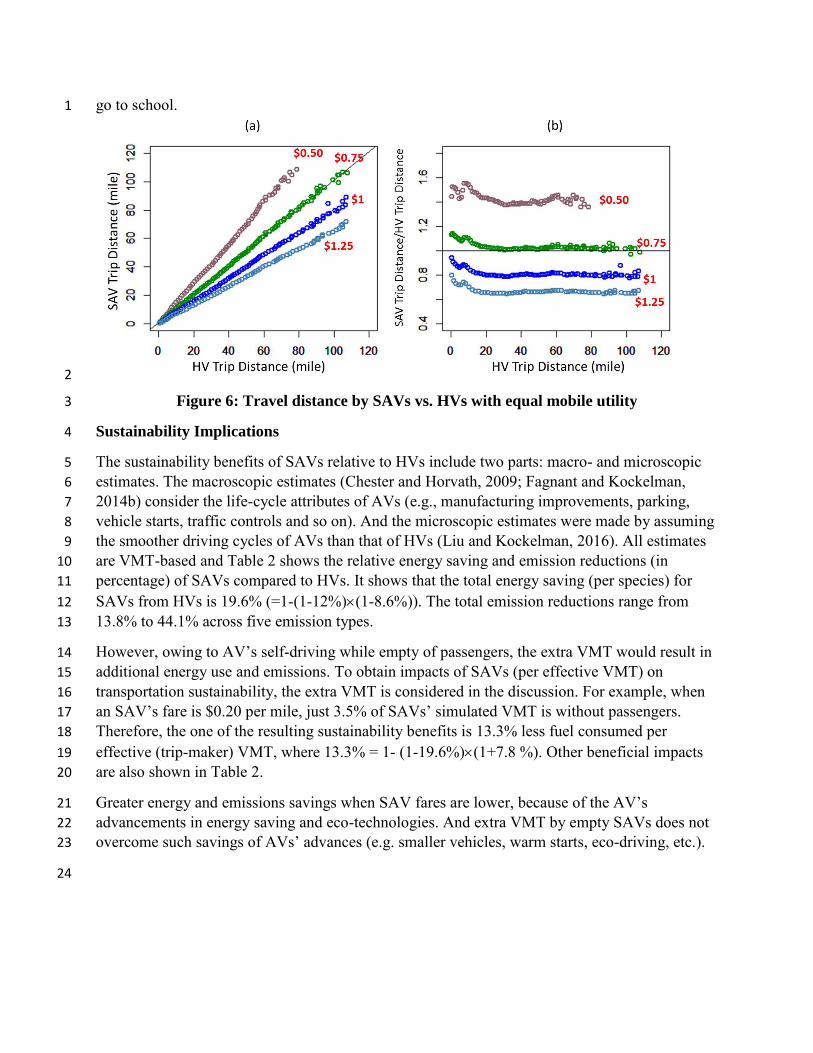
Mobility Implications 3

SAVs are expected to result in reduced travel burden (especially in vehicle portion), so that 4

travelers may travel to destinations that are farther away than current destinations without the 5

increase in comprehensive cost (including the out-of-pocket cost and relevant time spent during a 6

trip). Figure 6(a) shows controlling for the equal utility how far a SAV trip can reach given 7

certain HV trip distances. Figure 6(b) shows the ratio of distances of SAV trips and HV trips 8

with same utility. For SAV fare rate $0.5 per mile, travelers may travel 1.5 times longer 9

(respectively) using a SAV than using a HV with the same amount of paying (including the out-10

of-pocket cost and the VOT). When fare rate is $0.75 per mile (which is higher than the cost of 11

using a HV, $0.6 per mile), SAV travelers could travel similar distances with HV drivers, though 12

the distance-based cost for SAVs ($0.75 per mile) is be greater than the cost of using a HV ($0.6 13

per mile). While for two high fare rates, SAV trips tend to be shorter than HV trips, because of 14

the high out-of-pock cost of using a SAV. 15

Though SAVs with high fare rates do not increase the cost-equivalent distances of traveling (than 16

HVs), they are still expected to improve the mobility for certain group of people who are unable 17

to drive or walk to bus stations, such as people with disabilities, older fellows and children who 18

go to school. 1

2

Figure 6: Travel distance by SAVs vs. HVs with equal mobile utility 3

Sustainability Implications 4

The sustainability benefits of SAVs relative to HVs include two parts: macro- and microscopic 5

estimates. The macroscopic estimates (Chester and Horvath, 2009; Fagnant and Kockelman, 6

2014b) consider the life-cycle attributes of AVs (e.g., manufacturing improvements, parking, 7

vehicle starts, traffic controls and so on). And the microscopic estimates were made by assuming 8

the smoother driving cycles of AVs than that of HVs (Liu and Kockelman, 2016). All estimates 9

are VMT-based and Table 2 shows the relative energy saving and emission reductions (in 10

percentage) of SAVs compared to HVs. It shows that the total energy saving (per species) for 11

SAVs from HVs is 19.6% (=1-(1-12%)(1-8.6%)). The total emission reductions range from 12

13.8% to 44.1% across five emission types. 13

However, owing to AV’s self-driving while empty of passengers, the extra VMT would result in 14

additional energy use and emissions. To obtain impacts of SAVs (per effective VMT) on 15

transportation sustainability, the extra VMT is considered in the discussion. For example, when 16

an SAV’s fare is $0.20 per mile, just 3.5% of SAVs’ simulated VMT is without passengers. 17

Therefore, the one of the resulting sustainability benefits is 13.3% less fuel consumed per 18

effective (trip-maker) VMT, where 13.3% = 1- (1-19.6%)(1+7.8 %). Other beneficial impacts 19

are also shown in Table 2. 20

Greater energy and emissions savings when SAV fares are lower, because of the AV’s 21

advancements in energy saving and eco-technologies. And extra VMT by empty SAVs does not 22

overcome such savings of AVs’ advances (e.g. smaller vehicles, warm starts, eco-driving, etc.). 23

24

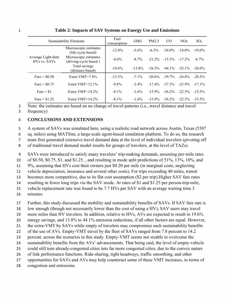
Table 2: Impacts of SAV Systems on Energy Use and Emissions 1

Sustainability Elements Fuel consumption GHG PM2.5 CO NOx SO2

Average Light-duty HVs vs. SAVs

Macroscopic estimates (life-cycle based) -12.0% -5.6% -6.5% -34.0% -18.0% -19.0%

Microscopic estimates (driving-cycle based ) -8.6% -8.7% -21.2% -15.3% -17.2% -8.7%

Total savings (distance-based) -19.6% -13.8% -26.3% -44.1% -32.1% -26.0%

Fare = $0.50 Extra VMT=7.8% -13.3% -7.1% -20.6% -39.7% -26.8% -20.3%

Fare = $0.75 Extra VMT=12.1% -9.8% -3.4% -17.4% -37.3% -23.9% -17.1%

Fare = $1 Extra VMT=14.2% -8.1% -1.6% -15.9% -36.2% -22.5% -15.5%

Fare = $1.25 Extra VMT=14.2% -8.1% -1.6% -15.9% -36.2% -22.5% -15.5%

Note: the estimates are based on no change of travel patterns (i.e., travel distance and travel 2 frequency) 3

CONCLUSIONS AND EXTENSIONS 4

A system of SAVs was simulated here, using a realistic road network across Austin, Texas (5307 5

sq. miles) using MATSim, a large-scale agent-based simulation platform. To do so, the research 6

team first generated extensive travel demand data at the level of individual travelers (pivoting off 7

of traditional travel demand model results for groups of travelers, at the level of TAZs). 8

SAVs were introduced to satisfy many travelers’ trip-making demands, assuming per-mile rates 9

of $0.50, $0.75, $1, and $1.25. , and resulting in mode split predictions of 51%, 13%, 10%, and 10

9%, assuming that HVs cost their owners just $0.20 per mile (in marginal costs, neglecting 11

vehicle depreciation, insurance and several other costs). For trips exceeding 40 miles, transit 12

becomes more competitive, due to its flat cost assumption ($2 per trip).Higher SAV fare rates 13

resulting in fewer long trips via the SAV mode. At rates of $1 and $1.25 per person-trip-mile, 14

vehicle replacement rate was found to be 7.7 HVs per SAV with an average waiting time 3 15

minutes. 16

Further, this study discussed the mobility and sustainability benefits of SAVs. If SAV fare rate is 17

low enough (though not necessarily lower than the cost of using a HV), SAV users may travel 18

more miles than HV travelers. In addition, relative to HVs, AVs are expected to result in 19.6% 19

energy savings, and 13.8% to 44.1% emission reductions, if all other factors are equal. However, 20

the extra-VMT by SAVs while empty of travelers may compromise such sustainability benefits 21

of the use of AVs. Empty-VMT travel by the fleet of SAVs ranged from 7.8 percent to 14.2 22

percent, across the scenarios in this study. Empty-VMT seems not sizable to overcome the 23

sustainability benefits from the AVs’ advancements. That being said, the level of empty-vehicle 24

could still turn already-congested cities into far more congested cities, due to the convex nature 25

of link performance functions. Ride-sharing, tight headways, traffic smoothing, and other 26

opportunities for SAVs and AVs may help counteract some of these VMT increases, in terms of 27

congestion and emissions. 28

While this study delivers insights for regional operations of SAV fleets, results can be improved 1

through continuing efforts. For example, this study’s results depend on the accuracy of 2

individuals’ travel activity patterns, and destination choices, which were generating using TAZ-3

level travel demand forecasts. The model of mode choice did not consider evolving HV 4

ownership levels and uneven cost of owning and operating a HV. 5

This study also assumed that travel requests with wait times longer than 10 minutes (total, from 6

request of service to vehicle arrival at trip-maker’s origin) could not be served. Such requests 7

may still be served if the traveler is patient enough, or the SAV managers (or companies) offers 8

discounted (or even free) rides for these travels in order to increase the ridership of the SAV 9

system. The extra VMT from access to AVs and SAVs may greatly influence traffic levels, as 10

AV prices fall and SAV fleet sizes grow. Moreover, dynamic feedback of traffic loads and travel 11

times to mode and destination choices is important for better understanding of coming 12

transportation system impacts and operations. 13

ACKNOWLEDGEMENTS 14

The authors would like to thank Texas Department of Transportation (TxDOT) for financially 15

supporting this research (under research project 6838, “Bringing Smart Transport to Texans: 16

Ensuring the Benefits of a Connected and Autonomous Transport System in Texas”). The 17

authors are grateful to the developers of MATSim for their consistent efforts in improving this 18

toolkit (available at http://www.matsim.org/). Special thanks to Scott Schauer-West, for his 19

constructive comments, edits, and administrative support. 20

REFERENCES 21

Anderson, J. M., K. Nidhi, K. D. Stanley, P. Sorensen, C. Samaras, and O. A. Oluwatola. 2014. 22

Autonomous Vehicle Technology: A Guide for Policymakers. Rand Corporation. Online at: 23

http://www.rand.org/pubs/research_briefs/RB9755.html?utm_source=t.co&utm_medium=rand_s24

ocial 25

Bansal, P., K. M. Kockelman, and Y. Wang. 2015. Hybrid Electric Vehicle Ownership and Fuel 26

Economy across Texas: An Application of Spatial Models. Transportation Research Record: 27

Journal of the Transportation Research Board, 2495: 53–64. 28

Barter, P. 2013. "Cars are parked 95% of the time". Let's check! Online at: 29

http://www.reinventingparking.org/2013/02/cars-are-parked-95-of-time-lets-check.html. 30

Bösch, P. M., F. Ciari, and K. W. Axhausen. 2016. Required Autonomous Vehicle Fleet Sizes to 31

Serve Different Levels of Demand. In: Transportation Research Board 95th Annual Meeting, 32

Online at: https://www.ethz.ch/content/dam/ethz/special-interest/baug/ivt/ivt-33

dam/vpl/reports/ab1089.pdf 34

CAMPO. 2015. CAMPO 2010 Planning Model Guide, Capital Area Metropolitan Planning 35

Organization (CAMPO), Austin, TX. Online at: http://www.campotexas.org/plans-programs/ 36

Census. 2014. ACS Profiles [dataset application]. Online at: 1

https://www.austintexas.gov/sites/default/files/files/Planning/Demographics/CoA_ACS_Profile_2

2013.pdf 3

Chapin, D., R. Brodd, G. Cowger, J. Decicco, G. Eads, R. Espino, J. German, D. Greene, J. 4

Greenwald, and L. Hegedus. 2013. Transitions to Alternative Vehicles and Fuels. National 5

Academies Press, Washington, DC. 6

Chen, D., and K. M. Kockelman. 2015. Management of a Shared, Autonomous, Electric Vehicle 7

Fleet: Charging and Pricing Strategies. In: IATBR 2015-WINDSOR. Online at: 8

http://www.caee.utexas.edu/prof/kockelman/public_html/TRB16SAEVsModeChoice.pdf 9

Chen, D., K. M. Kockelman, and J. Hanna. 2016. Operations of a Shared, Autonomous, Electric 10

Vehicle (SAEV) Fleet: Implications of Vehicle & Charging Infrastructure Decisions In: 11

Transportation Research Board 95th Annual Meeting. Online at: 12

http://www.caee.utexas.edu/prof/kockelman/public_html/TRB16SAEVs100mi.pdf 13

Chester, M., and A. Horvath. 2009. Life-cycle energy and emissions inventories for motorcycles, 14

diesel automobiles, school buses, electric buses, Chicago rail, and New York City rail. UC 15

Berkeley Center for Future Urban Transport: A Volvo Center of Excellence. Online at: 16

http://www.its.berkeley.edu/sites/default/files/publications/UCB/2009/VWP/UCB-ITS-VWP-17

2009-2.pdf 18

Ciari, F., M. Balac, and K. W. Axhausen. 2016. Modeling carsharing with the agent-based 19

simulation MATSim: state of the art, applications and future developments. In: Transportation 20

Research Board 95th Annual Meeting. Online at: http://e-21

citations.ethbib.ethz.ch/view/pub:161004 22

Fagnant, D. J., and K. Kockelman. 2014a. Preparing a Nation for Autonomous Vehicles: 23

Opportunities, Barriers and Policy Recommendations for Capitalizing On Self-Driven Vehicles. 24

Transportation Research Part A 77: 167-181, 2015. 25

Fagnant, D. J., and K. M. Kockelman. 2014b. The travel and environmental implications of 26

shared autonomous vehicles, using agent-based model scenarios. Transportation Research Part 27

C: Emerging Technologies 40: 1-13. 28

Fagnant, D. J., and K. M. Kockelman. 2015. Dynamic ride-sharing and optimal fleet sizing for a 29

system of shared autonomous vehicles. Forthcoming in Transportation. Online at: 30

http://www.caee.utexas.edu/prof/kockelman/public_html/TRB15SAVswithDRSinAustin.pdf 31

Folsom, T. 2012. Energy and autonomous urban land vehicles. IEEE Technology and Society 32

Magazine 2: 28-38. 33

Ford. 2012. Model T Facts. Online at: 34

https://media.ford.com/content/fordmedia/fna/us/en/news/2013/08/05/model-t-facts.html 35

Gagnier, S. 2013. Car sharing users to reach 12 million by 2020, report says. Online at: 1

http://www.autonews.com/article/20130916/OEM06/130919868/car-sharing-users-to-reach-12-2

million-by-2020-report-says. 3

Google. 2016. Google Self-Driving Car Project. Online at: 4

https://www.google.com/selfdrivingcar/ 5

Horni, A., D. Scott, M. Balmer, and K. Axhausen. 2009. Location choice modeling for shopping 6

and leisure activities with MATSim: combining microsimulation and time geography. 7

Transportation Research Record: Journal of the Transportation Research Board 2135: 87-95. 8

Kockelman, K. M., and T. Li. 2016. Valuing the Safety Benefits of Connected and Automated 9

Vehicle Technologies. In: Transportation Research Board 95th Annual Meeting. Online at: 10

http://www.caee.utexas.edu/prof/kockelman/public_html/TRB16CAVSafety.pdf 11

Leob, B., K. Kockelman and J. Liu. 2016. Shared Autonomous Electric Vehicles (SAEV) 12

Operations across the Austin, Texas Network with a Focus on Charging Infrastructure Decisions. 13

Under review for publication in Transportation Research Record. 14

Liu, J., A. Khattak, and X. Wang. 2015. The role of alternative fuel vehicles: Using behavioral 15

and sensor data to model hierarchies in travel. Transportation Research Part C: Emerging 16

Technologies 55: 379-392. 17

Liu, J., K. Kockelman, and A. Nichols. 2016. Anticipating the Emissions Impacts Of Connected 18

and Autonomous Vehicles Using the MOVES Model. Under review for publication in 19

Transportation Research Record. Online at: 20

http://www.caee.utexas.edu/prof/kockelman/public_html/TRB17emissionsAVsmoothedcycle.pdf 21

Maciejewski, M., and K. Nagel. 2013. Simulation and dynamic optimization of taxi services in 22

MATSim, VSP Working Paper 13-05, TU Berlin, Transport Systems Planning and Transport 23

Telematics. Online at: http://svn.vsp.tu-berlin.de/repos/public-svn/publications/vspwp/2013/13-24

05/2013-06-03_Maciejewski_Nagel.pdf 25

MATSim. 2016a. MATSim | Multi-Agent Transport Simulation. Online at: 26

http://www.matsim.org/scenarios. 27

MATSim. 2016b. The MATSim Book. Online at: http://www.matsim.org/the-book 28

Capital Metropolitan Transportation Authority. 2010. ServicePlan2020 [Draft Final Report], 29

Capital Metropolitan Transportation Authority. Online at: 30

http://www.capmetro.org/uploadedFiles/Capmetroorg/Future_Plans/Service_Plan_2020/ServiceP31

lan2020%20-%20Final%20Report.pdf 32

Capital Metropolitan Transportation Authority. 2016. Capital Metro of Austin. 33

http://www.capmetro.org/ 34

NCHRP. 2012. Travel Demand Forecasting: Parameters and Techniques. National Cooperative 35

Highway Research Program, Transportation Research Board. Online at: 36

http://onlinepubs.trb.org/onlinepubs/nchrp/nchrp_rpt_716.pdf 37

Novosel, T., L. Perković, M. Ban, H. Keko, T. Pukšec, G. Krajačić, and N. Duić. 2015. Agent 1

based modelling and energy planning–Utilization of MATSim for transport energy demand 2

modelling. Energy 92: 466-475. 3

Paul, B., K. Kockelman, and S. Musti. 2011. Evolution of the light-duty vehicle fleet: 4

anticipating adoption of plug-In hybrid electric vehicles and greenhouse gas emissions across the 5

US fleet. Transportation Research Record: Journal of the Transportation Research Board 2252: 6

107-117. 7

Reiter, M. S., and K. M. Kockelman. 2016. Emissions and Exposure Costs of Electric Versus 8

Conventional Vehicles: A Case Study for Texas. In: Transportation Research Board 95th 9

Annual Meeting. Online at: 10

http://www.caee.utexas.edu/prof/kockelman/public_html/TRB16Emissions&Exposure.pdf 11

Santos, A., N. McGuckin, H. Y. Nakamoto, D. Gray, and S. Liss. 2011. Summary of Travel 12

Trends: 2009 National Household Travel Survey. Online at: http://nhts.ornl.gov/2009/pub/stt.pdf 13

Schrank, D., B. Eisele, T. Lomax, and J. Bak. 2015. 2015 Urban Mobility Scorecard Texas 14

A&M Transportation Institute & INRIX, Inc., Colleage Station, TX. Online at: 15

http://d2dtl5nnlpfr0r.cloudfront.net/tti.tamu.edu/documents/mobility-scorecard-2015.pdf 16

Tomlinson, C. 2016. Car-sharing expected to rise dramatically. Online at: 17

http://www.houstonchronicle.com/business/outside-the-boardroom/article/Car-sharing-expected-18

to-rise-dramatically-7511140.php 19

TxDOT. 2015. Roadway Inventory Data. Online at: http://www.txdot.gov/inside-20

txdot/division/transportation-planning/roadway-inventory.html. 21

Uber. 2016. Steel City’s New Wheels. Online at: https://newsroom.uber.com/us-22

pennsylvania/new-wheels/. 23