Introduction Theory Testable Implications Data and Methodology Results conclusion

Toxic Arbitrage

Thierry FoucaultHEC

Roman KozhanUniversity of Warwick

Wing Wah ThamErasmus University Rotterdam

American Finance Association MeetingsJanuary 5, 2015

Introduction Theory Testable Implications Data and Methodology Results conclusion

Goal of the paper

� What is the effect of high speed arbitrage on liquidity?

� Why is this question important and interesting?

Introduction Theory Testable Implications Data and Methodology Results conclusion

Highly Profitable

� What is the value of these trades for arbitrageurs’counterparties?

Introduction Theory Testable Implications Data and Methodology Results conclusion

Regulatory Concerns

� SEC (2010): ”U.S. concept release on equity marketstructure.”

“ The Commission requests comment on arbitragestrategies and whether they benefit or harm theinterests of long-term investors and market quality ingeneral.[...]” (Securities Exchange Commission,2010)

� Yet no analysis of the effects of high frequency arbitragebecause lack of data on cross-market trades by HFTs:

“The literature does not reveal a great deal aboutthe extent of the HFT arbitrage strategies [...] ”(Securities Exchange Commission, 2014)

Introduction Theory Testable Implications Data and Methodology Results conclusion

Arbitrage = Cornerstone of Financial Economics

� ”To make a parrot into a learned financial economist, heonly needs to learn the single word: “arbitrage” (Ross(1987, American Economic Review)

� What is the social value of high speed arbitrage?� Traditional view:

1. Arbitrageurs increase pricing efficiency: they quicklycorrect mispricings due to noise/liquidity traders.

2. Arbitrageurs are like liquidity providers (literature onlimits to arbitrage). In correcting mispricing, they provideliquidity to noise/liquidity traders =⇒ ”Relaxing constraintsshould be desirable because arbitrageurs provide liquidity”(Gromb and Vayanos (2012))

� Our paper: Some arbitrage opportunities (not all) raiseadverse selection costs ⇒ they can make markets less liquid.

� Why?

Introduction Theory Testable Implications Data and Methodology Results conclusion

Arbitrage 1: Stale Quotes.

Introduction Theory Testable Implications Data and Methodology Results conclusion

Arbitrage 2: Transient Price Pressures.

Introduction Theory Testable Implications Data and Methodology Results conclusion

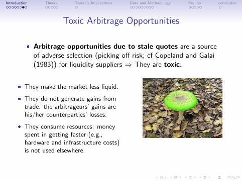
Toxic Arbitrage Opportunities

� Arbitrage opportunities due to stale quotes are a sourceof adverse selection (picking off risk; cf Copeland and Galai(1983)) for liquidity suppliers ⇒ They are toxic.

� They make the market less liquid.

� They do not generate gains fromtrade: the arbitrageurs’ gains arehis/her counterparties’ losses.

� They consume resources: moneyspent in getting faster (e.g.,hardware and infrastructure costs)is not used elsewhere.

Introduction Theory Testable Implications Data and Methodology Results conclusion

Testable Predictions

� ”Composition effect:” This is

not the number of arbitrage

opportunities that matters but

the nature of these opportunities.

Illiquidity is higher

1. On days in which toxicarbitrage opportunities aremore frequent;

2. In pairs of related assets(ETFs/Underlying basket) inwhich toxic opportunities aremore frequent.

� ”Speed effect”: Illiquidity is higher when arbitrageursreact faster to toxic arbitrage opportunities.

Introduction Theory Testable Implications Data and Methodology Results conclusion

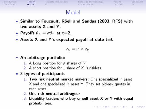
Model

� Similar to Foucault, Roell and Sandas (2003, RFS) withtwo assets X and Y.

� Payoffs θX = σθY at t=2.

� Assets X and Y’s expected payoff at date t=0

vX = σ× vY

� An arbitrage portfolio:1. A Long position for σ shares of Y2. A short position for 1 share of X is riskless.

� 3 types of participants1. Two risk neutral market makers: One specialized in asset

X and one specialized in asset Y. They set bid-ask quotes ineach asset.

2. One risk neutral arbitrageur3. Liquidity traders who buy or sell asset X or Y with equal

probabilities.

Introduction Theory Testable Implications Data and Methodology Results conclusion

Case 1: Stale Quotes.

Introduction Theory Testable Implications Data and Methodology Results conclusion

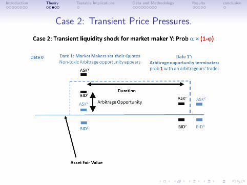
Case 2: Transient Price Pressures.

Introduction Theory Testable Implications Data and Methodology Results conclusion

The Arbitrage Race

� Traders choose their average speed of reaction (”latency”) to arbitrageopportunities λ−1 or γ−1) but being faster is costly.

� π = A measure of arbitrageurs’ relative speed.

Introduction Theory Testable Implications Data and Methodology Results conclusion

Equilibrium

� Not a standard adverse selection problem because π dependson speeds choices, which in turn depend on the bid-ask spread

� =⇒ Spreads, traders’ speeds (π), and the duration of anarbitrage opportunity (a measure of pricing efficiency).

� We solve for equilibrium spreads, speeds, duration of arbitrageopporunities and π∗ and obtain 4 testable implications.

Introduction Theory Testable Implications Data and Methodology Results conclusion

Testable implications

� Imp.1a: An increase in the fraction of arbitrage opportunitiesthat are toxic (ϕ) causes an increase in illiquidity.

� Imp.1b: An increase in arbitrageurs’ speed relative to dealers’speed (π) causes an increase in illiquidity.

� Imp.2: A decrease in the cost of speed (a reduction in cd orca) reduces the duration of arbitrage opportunities.

� Imp.3: An increase in the fraction of arbitrage opportunitiesthat are toxic (ϕ) causes a reduction in the duration ofarbitrage opportunities.

→ Faster arbitrageurs’ reactions to toxic arbitrage opportunitiesmake the market less liquid but always more price efficient.

Introduction Theory Testable Implications Data and Methodology Results conclusion

Triangular Arbitrage

Introduction Theory Testable Implications Data and Methodology Results conclusion

Triangular Arbitrage Opportunities

Two ways to buy euros with dollar:� Direct: Buy e1 at A$/e, the ask price in dollar for euros

Cost: A$/e

� Indirect: Buy A£/e units of pounds at A$/£ and then e1 at A£/e in theeuro/sterling market

Cost: A$/e=A£/e×A$/£

Two ways to sell euros against dollar:� Direct: Sell e1 at B$/e, the bid price in dollar for euros

Revenue: B$/e

� Indirect: Sell e1 at B£/e in the euro/sterling market and then sell B£/e

units of pounds at B$/£

Revenue: B$/e=B£/e×B$/£

A triangular arbitrage opportunity exists if:Ask$/e < Bid

$/eor Ask

$/e< Bid$/e

Introduction Theory Testable Implications Data and Methodology Results conclusion

Data� Tick-by-tick data (2003-2004) from Reuters D-3000: an interdealer

limit order book in the FX market

� Three currency pairs: $/e, $/£ and e/£

� All orders: limit, market, cancellations etc

� Time-stamped accuracy at the one-hundredth of a second

Triangular arbitrage in the FX market� short-lived (last for about 1 second and sometimes much less)

� almost riskless

� deliver a very small profit per opportunity

� large number of triangular arbitrage opportunities in our sample(37,689 over two years)

� similar in nature to opportunities exploited by HF arbitrageurs

Introduction Theory Testable Implications Data and Methodology Results conclusion

Toxic vs. Non-Toxic Arbitrage opportunities: Classification

Panel A: Toxic arbitrage opportunities (permanent shifts in prices)

Panel B: Non-toxic arbitrage opportunities (price reversals)

� # toxic triangular arbitrages in sample: 15,908.

Introduction Theory Testable Implications Data and Methodology Results conclusion

Toxic and Non Toxic Arbitrage Opportunities: Time-Series

Introduction Theory Testable Implications Data and Methodology Results conclusion

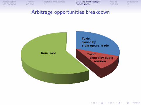
Arbitrage opportunities breakdown

Introduction Theory Testable Implications Data and Methodology Results conclusion

Proxies for Dealers’ Exposure to Toxic Arbitrage Trades

ϕt =# Toxic arbitrage opportunities on day t

# Arbitrage opportunities on day t.

πt =# Toxic opportunities closed by a trade on day t

# Toxic Arbitrage opportunities on day t

� Reminder:1. If toxic arbitrage opportunities end up more frequently with an

arbitrageur’s trade, arbitrageurs tend to be faster.

2. Thus, days in which πt is high, are days in which arbitrageursare relatively faster.

Introduction Theory Testable Implications Data and Methodology Results conclusion

Toxic vs. Non-Toxic Arbitrage opportunities

Toxic Non Toxic

Daily measures Median SD Median SD

Duration (msd) 890 0.30 510 0.2

Nbr Arb 32 20 45 38

ϕ(%) 41.5 10 59 11

Arb Size (bps) 3.53 0.75 3.53 0.84

Profit (bps) 1.42 0.27 1.61 0.57

π (%) 74 11 80 8.2

� Profit per opportunity are small but the total daily profit on

triangular arbitrages (about $5,000) is of the order of magnitude of

that found for HFTs on Nasdaq (see Brogaard, Hendershott and

Riordan (2012)).

� π for toxic and non toxic arbitrage opportunities have a zero

correlation (0.08) =⇒ do not capture the same phenomenon.

Introduction Theory Testable Implications Data and Methodology Results conclusion

Liquidity measures

� Other control variables: daily realized volatility, daily average

arbitrage profit, daily average trade size in millions, daily number of

orders, illiquidity on EBS platform

Introduction Theory Testable Implications Data and Methodology Results conclusion

Main Test

� We estimate the following regression for the three currenciesin our sample:

Illit = αi + βt + b1πt + b2 ϕt + b3Volit + b4Arbsizet

+ b5Trsizeit + b6#Ordersit + b7IlliqEBSit + εit

Predictions: b1 > 0 and b2 > 0.

Introduction Theory Testable Implications Data and Methodology Results conclusion

IV Approach

� Reverse Causality Problem: Illiquidity also affects π:Arbitrageurs have less incentive to be fast when trading costsare large.

� Proper econometric analysis requires an exogenous shock onπ (an “instrument”), i.e., one that affects participants’ speedwithout directly affecting liquidity.

� We use the introduction of “AutoQuote ” (API) by ReutersD-3000 in July 2003 as an instrument.

� AutoQuote API (Application Programming Interface): Enabletraders using Reuters D-3000 to automate order entry basedon Reuters D-3000 datafeed ⇒ onset of algo trading onReuters.

� ⇔ Increase in traders’ speed. Should affect π withoutdirectly affecting illiquidity.

Introduction Theory Testable Implications Data and Methodology Results conclusion

Findings

spread espread slope

1st stage 2nd stage 1st stage 2nd stage 1st stage 2nd stage

AD 0.040 (4.09) 0.042 (4.12) 0.040 (4.10)

π 7.934 (3.91) 3.443 (3.70) 4.526 (3.96)

ϕ -0.011 (-0.31) 0.691 (2.29) -0.011 (-0.31) 0.511 (3.68) -0.010 (-0.28) 0.445 (2.61)

σ -0.011 (-2.14) 0.238 (4.93) -0.012 (-2.17) 0.221 (9.94) -0.011 (-2.11) 0.120 (4.39)

vol -0.009 (-0.75) 0.374 (3.72) -0.009 (-0.77) 0.401 (8.65) -0.009 (-0.76) 0.220 (3.87)

trsize 0.002 (0.66) -0.128 (-0.30) 0.001 (0.84) -0.196 (-0.98) 0.001 (0.76) -0.265 (-1.09)

nrorders 0.014 (0.27) -0.004 (-0.77) 0.012 (0.22) -0.006 (-2.62) 0.016 (0.30) -0.003 (-1.01)

illiqEBS -0.003 (-3.88) 0.021 (0.79) -0.003 (-3.85) -0.002 (-0.43) -0.003 (-3.89) 0.001 (0.08)

Adj .R2 2.34% 34.40% 2.34% 62.18% 2.35% 25.56%

Fstat 16.7 16.9 16.8

Currencypair FE

YES YES YES

Monthdummies

YES YES YES

Introduction Theory Testable Implications Data and Methodology Results conclusion

Economic size of the effects� A 1% increase in the likelihood that a toxic arbitrage terminates

with an arbitrageur’s trade (π) raises bid-ask spread by about 4%(0.08bps)

� This effect translates in a quite large increase in trading costs given

the trading volume for the currencies in our sample (average trade

size of about 1.8 mio with about 2,500 trades per day). We

estimate that the increase in trading costs due to a 1% increase in:

� π is $161,296 (about $40 mio per year)

� ϕ is $ 14,047 (the daily standard deviation of ϕ is 10%)

� As a point of comparison: Naranjo and Nimalendran (2000)

estimates at $55 mio the annualized cost of German and U.S central

banks intervention in the DM/$ market

Introduction Theory Testable Implications Data and Methodology Results conclusion

Arbitrage and Pricing Efficiency (Implications 3 and 4)

Dep.Var: log(TTE ) Toxic All

AD -0.068 (-3.04) -0.057 (-2.93)

vol -0.084 (-3.15) -0.105 (-4.53)

ϕ -0.248 (-2.95) 0.050 (0.68)

σ 0.070 (6.59) 0.085 (9.22)

trsize 0.022 (0.18) 0.015 (0.14)

nrorders -0.012 (-7.29) -0.010 (-7.40)

Adj .R2 21.24% 33.33%

� The introduction of “Automated Order Entry” reduces by

about 0.06 sd the duration of arbitrage opportunities (about

5.6% of the median duration of toxic arbitrage opportunities).

Introduction Theory Testable Implications Data and Methodology Results conclusion

Conclusions

� Arbitrage and liquidity:1. The mix of arbitrage opportunities matters: more arbitrage

opportunities due asynchronous price adjustments areassociated with less liquidity.

2. Faster arbitrageurs’ reaction to these opportunities → lowerliquidity.

� Future Work: What is the social benefit of high speedarbitrageurs?

1. Faster price discovery? Do we care about prices being right 60ms faster? Why?

2. Faster response to transient liquidity shocks? Maybe...needs tobe modeled and quantified, however.