The Mathematics of Geographic Profiling

Towson UniversityApplied Mathematics Laboratory

Dr. Mike O'Leary

Crime Hot Spots: Behavioral, Computational and Mathematical ModelsInstitute for Pure and Applied Mathematics

January 29 - February 2, 2007

Supported by the NIJ through grant 2005–IJ–CX–K036

Project Participants

Towson University Applied Mathematics Laboratory

Undergraduate research projects in applied mathematics.

Founded in 1980

National Institute of Justice

Special thanks to Stanley Erickson (NIJ) and Andrew Engel (SAS)

Students

2005-2006:Paul Corbitt

Brooke Belcher

Brandie Biddy

Gregory Emerson

2006-2007:Chris Castillo

Adam Fojtik

Laurel Mount

Ruozhen Yao

Melissa Zimmerman

Jonathan Vanderkolk

Grant Warble

Geographic Profiling

The Question:

Given a series of linked crimes committed by the same offender, can we make predictions about the anchor point of the offender?

The anchor point can be a place of residence, a place of work, or some other commonly visited location.

Geographic Profiling

Our question is operational.

This places limitations on available data.

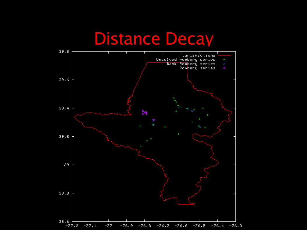
Example

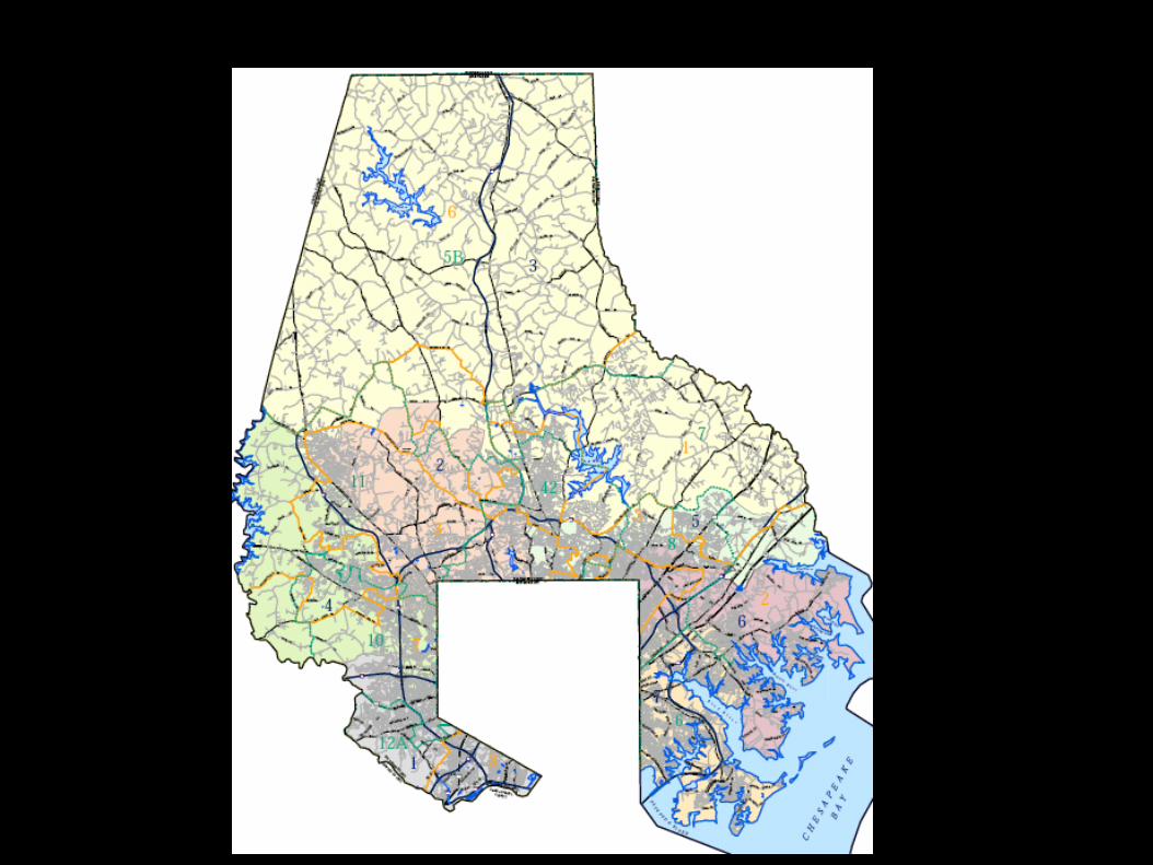
A series of 9 linked vehicle thefts in Baltimore County

Example

ADDRESS DATE_FROM TIME DATE_TO TIME REMARKS

918 M 01/18/2003 0800 01/18/2003 0810 VEHICLE IS 01 TOYT CAMRY,LEFT VEH RUNNING

1518 L 01/22/2003 0700 01/22/2003 0724 VEHICLE IS 99 HOND ACCORD STL-REC, ...B/M PAIR,DRIVING MAROON ACCORD.

731 CC 01/22/2003 0744 01/22/2003 0746 VEHICLE IS 02 CHEV MALIBU STL-REC

1527 K 01/27/2003 1140 01/27/2003 1140 VEHICLE IS 97 MERC COUGAR, LEFT VEH RUNNING

1514 G 01/29/2003 0901 01/29/2003 0901 VEHICLE IS 99 MITS DIAMONTE, LEFT VEH RUNNING

1415 K 01/29/2003 1155 01/29/2003 1156 VEHICLE IS 00 TOYT 4RUNNER STL-REC, (4) ARREST NFI

5943 R 12/31/2003 0632 12/31/2003 0632 VEHICLE IS 92 BMW 525, WARMING UP VEH

1427 G 02/17/2004 0820 02/17/2004 0830 VEHICLE IS 00 HOND ACCORD, WARMING VEH

4449 S 05/15/2004 0210 05/15/2004 0600 VEHICLE IS 04 SUZI ENDORO

Existing Methods

Spatial distribution strategies

Probability distance strategies

Notation:

Anchor point-

Crime sites-

Number of crimes-

z= z 1 , z 2x1 , x2 ,⋯ , xn

n

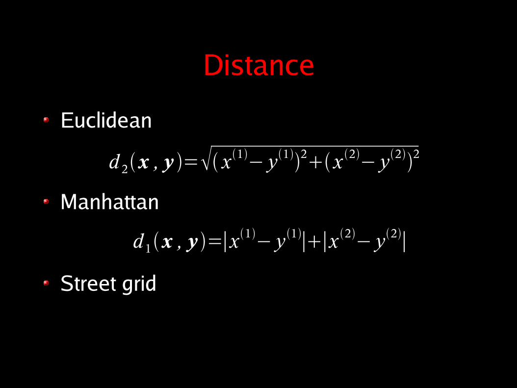
Distance

Euclidean

Manhattan

Street grid

d1x , y =∣x1− y1∣∣x 2− y2∣

d 2x , y = x1− y12 x 2− y22

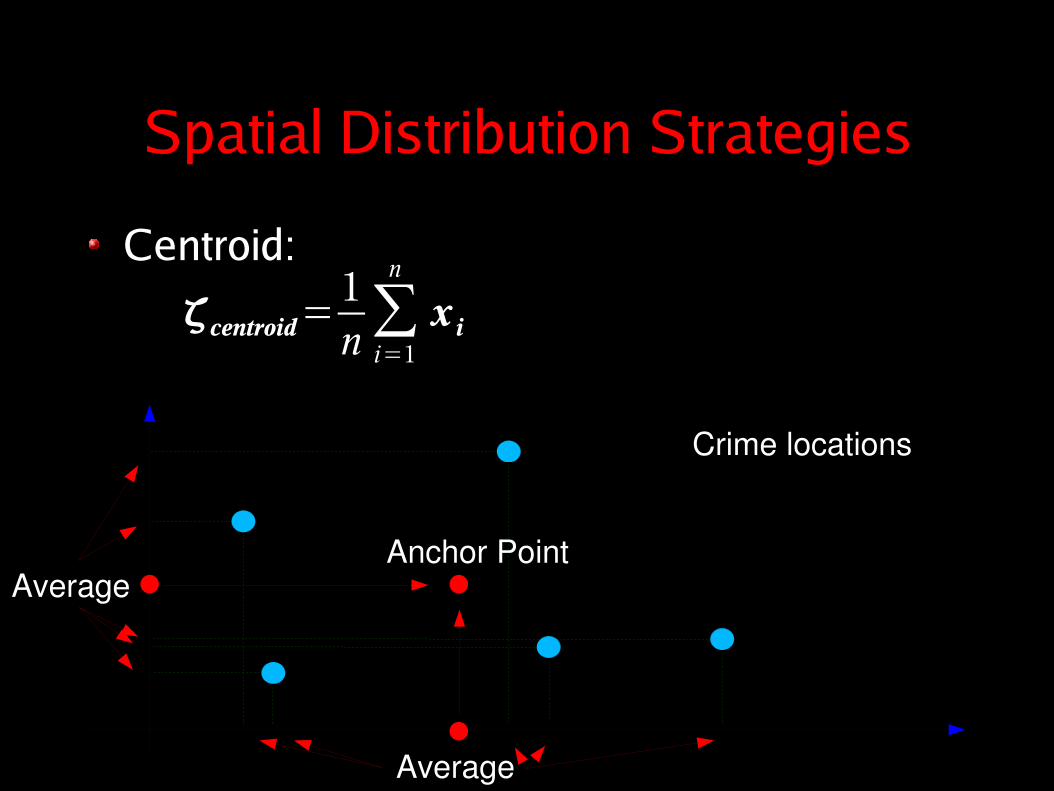
Spatial Distribution Strategies

Centroid:

Crime locations

Average

Average

Anchor Point

centroid=1n∑i=1

n

x i

Spatial Distribution Strategies

Center of minimum distance: is the value of that minimizes

Crime locations

Distance sum = 10.63

Distance sum = 9.94

Smallest possible sum!

Anchor Point

cmdy

D y =∑i=1

n

d x i , y

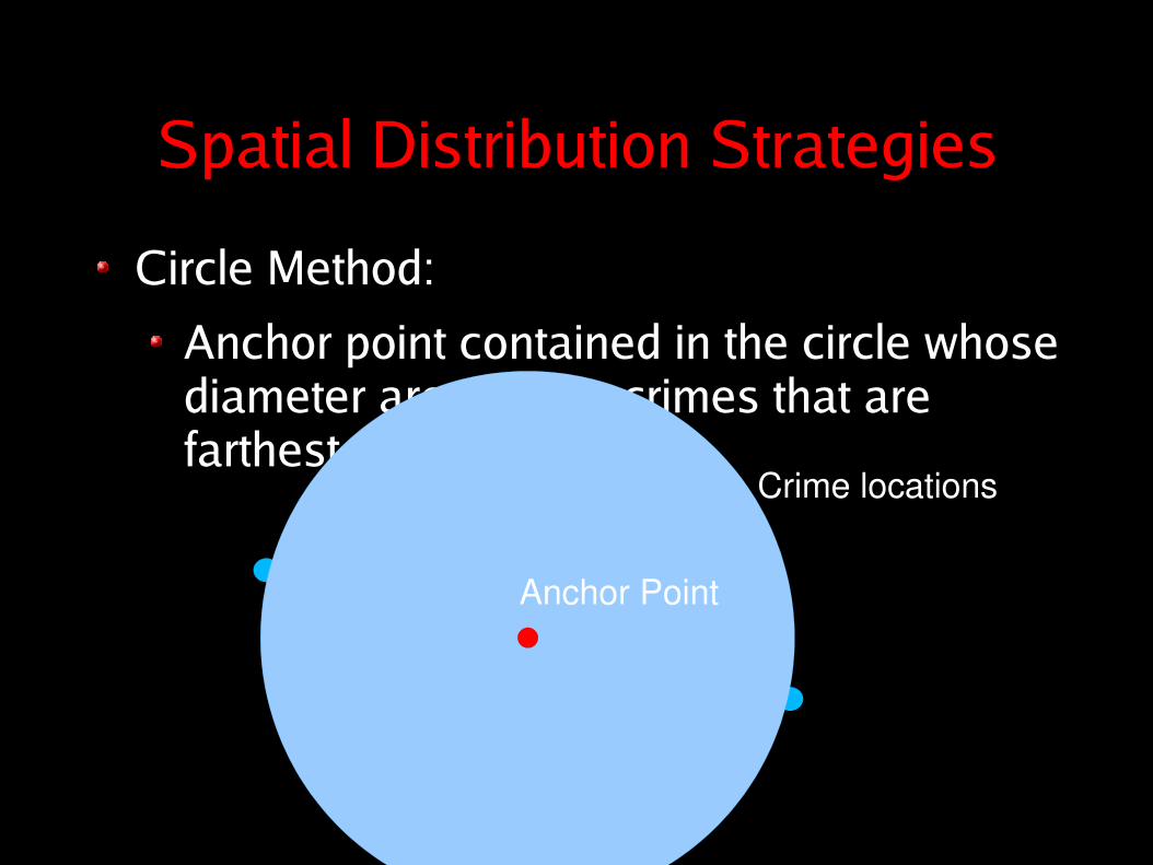
Spatial Distribution Strategies

Circle Method:

Anchor point contained in the circle whose diameter are the two crimes that are farthest apart.

Crime locations

Anchor Point

Probability Distribution Strategies

The anchor point is located in a region with a high “hit score”.

The hit score has the form

where are the crime locations and is a decay function and is a distance.

S y =∑i=1

n

f d y , xi

S y

= f d z , x1 f d z , x2⋯ f d z , xn

xi fd

Probability Distribution Strategies

Linear:

f d =A−Bd

Hit Score

Crime Locations

Rossmo

Manhattan distance metric.

Decay function

The constants and are empirically defined

f d ={kd h if dB

k Bg−h

2B−d gif dB

k , g ,h B

Rossmo

B=1h=2g=3

Canter, Coffey, Huntley & Missen

Euclidean distance

Decay functions

f d =Ae−d

f d ={ 0 if dA ,B if A≤dB

Ce−d if d≥B .,

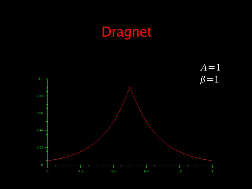
Dragnet

A=1=1

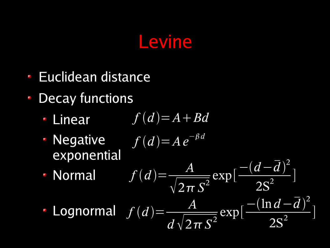
Levine

Euclidean distance

Decay functions

Linear

Negative exponential

Normal

Lognormal

f d =ABd

f d =Ae−d

f d = A

2 S2exp [−d−

d 2

2S2 ]

f d = A

d 2S 2exp[−lnd−

d 2

2S2 ]

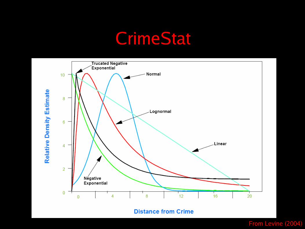
CrimeStat

From Levine (2004)

CrimeStat

Shortcomings

These techniques are all ad hoc.

What is their theoretical justification?

What assumptions are being made about criminal behavior?

What mathematical assumptions are being made?

How do you choose one method over another?

Shortcomings

The convex hull effect:

The anchor point always occurs inside the convex hull of the crime locations.

Crime locations

Convex Hull

Shortcomings

How do you add in local information?

How could you incorporate socio-economic variables into the model?

Snook, Individual differences in distance travelled by serial burglars

Malczewski, Poetz & Iannuzzi, Spatial analysis of residential burglaries in London, Ontario

Bernasco & Nieuwbeerta, How do residential burglars select target areas?

Osborn & Tseloni, The distribution of household property crimes

A New Approach

In previous methods, the unknown quantity was:

The anchor point (spatial distribution strategies)

The hit score (probability distance strategies)

We use a different unknown quantity.

A New Approach

Let be the density function for the probability that an offender with anchor point commits a crime at location .

This distribution is our new unknown.

This has criminological significance.

In particular, assumptions about the form of are equivalent to assumptions about the offender's behavior.

P x ; z

z x

P x ; z

The Mathematics

Given crimes located at the maximum likelihood estimate for the anchor point is the value of that maximizes

or equivalently, the value that maximizes

x1 , x2 ,⋯, xn

mle y

L y =∏i=1

n

P x i , y

=P x1 , yP x2 , y ⋯P xn , y

y=∑i=1

n

ln P x i , y

=ln P x1 , yln P x2 , y ⋯ln P xn , y

Relation to Spatial Distribution Strategies

If we make the assumption that offenders choose target locations based only on a distance decay function in normal form, then

The maximum likelihood estimate for the anchor point is the centroid.

P x ; z = 1

22 exp[−∣x−z∣222 ]

Relation toSpatial Distribution Strategies

If we make the assumption that offenders choose target locations based only on a distance decay function in exponentially decaying form, then

The maximum likelihood estimate for the anchor point is the center of minimum distance.

P x ; z = 122 exp [−∣x−z∣2 ]

Relation toProbability Distance StrategiesWhat is the log likelihood function?

This is the hit score provided we use Euclidean distance and the linear decay for

y =∑i=1

n [−ln 22−∣x i− y∣ ]

S y

f d =ABdA=−ln 22B=−1 /

Parameters

The maximum likelihood technique does not require a priori estimates for parameters other than the anchor point.

The same process that determines the best choice of also determines the best choice of .

P x ; z ,= 1

22 exp [−∣x−z∣222 ]z

Better Models

We have recaptured the results of existing techniques by choosing appropriately.

These choices of are not very realistic.

Space is homogeneous and crimes are equi-distributed.

Space is infinite.

Decay functions were chosen arbitrarily.

P x ; z

P x ; z

Better Models

Our framework allows for better choices of .

Consider

P x ; z

P x ; z =D d x , z ⋅G x ⋅N z

Geographicfactors

NormalizationDistance Decay (Dispersion Kernel)

The Simplest Case

Suppose we have information about crimes committed by the offender only for a portion of the region.

W

E

The Simplest Case

Regions

: Jurisdiction(s). Crimes and anchor points may be located here.

E: “elsewhere”. Anchor points may lie here, but we have no data on crimes here.

W: “water”. Neither anchor points nor crimes may be located here.

In all other respects, we assume the geography is homogeneous.

The Simplest Case

We set

We choose an appropriate decay function

The required normalization function is

G x ={1 x∈0 x∉

D ∣x−z∣=exp [−∣x−z∣222 ]N x ; z=[∬ exp −∣y− z∣2

22 dy1dy2]−1

The Simplest Case

Our estimate of the anchor point is the choice of that maximizes

exp −∑i=1

n ∣x i− y∣2

22 [∬ exp −∣− y∣222 d 1d 2]

n

mle

y

The Simplest Case

Our students wrote code to implement this method last year, and tested it on real crime data from Baltimore County.

We used Green's theorem to convert the double integral to a line integral.

Baltimore county was simply a polygon with 2908 vertices.

∬

exp −∣− y∣222 d 1d2=∮∂

− 2

∣− y∣exp−∣− y∣2β e r⋅n ds{βπ z∈

0 z∉

The Simplest Case

To calculate the maximum, we used the BFGS method.

Search in the direction where

For the 1-D optimization we used the bisection method.

Dn∇ f yn

Dn1=Dn1 gT Dn g

d T g ddTdT g−Dn gd

TgdT DndT g

d= yn1− yng=∇ f yn1−∇ f yn

Sample ResultsBaltimore CountyVehicle TheftPredicted Anchor PointOffender's Home

Better Models

This is just a modification of the centroid method that accounts for possibly missing crimes outside the jurisdiction.

Clearly, better models are needed.

Better Models

Recall our ansatz

What would be a better choice of ?

What would be a better choice of ?

P x ; z =D d x , z ⋅G x ⋅N z

D

G

Distance Decay

From Levine (2004)

Distance Decay

Distance Decay

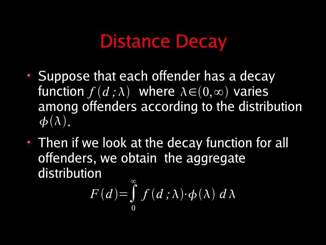
Suppose that each offender has a decay function where varies among offenders according to the distribution .

Then if we look at the decay function for all offenders, we obtain the aggregate distribution

f d ; ∈0,∞

F d =∫0

∞

f d ;⋅ d

Distance Decay

f d = A

d 2S 2exp [− ln d−

d 2

2 S 2 ]

A=d=0.1

Scaling ParametersShape Parameters

0.51234}=2 S 2

Distance Decay

1 2 3 4 5x

0.2

0.4

0.6

0.8

Aggregate Distrbution

Each offender has a lognormal decay functionThe offender's shape parameter has a lognormal decay

1 2 3 4 5x

0.2

0.4

0.6

0.8

Aggregate Distrbution

Distance Decay

Distance Decay

Is this real, or an artifact?

How do we determine the “best” choice of decay function?

This needs to be determined in advance.

Will it vary depending on

crime type?

local geography?

Geography

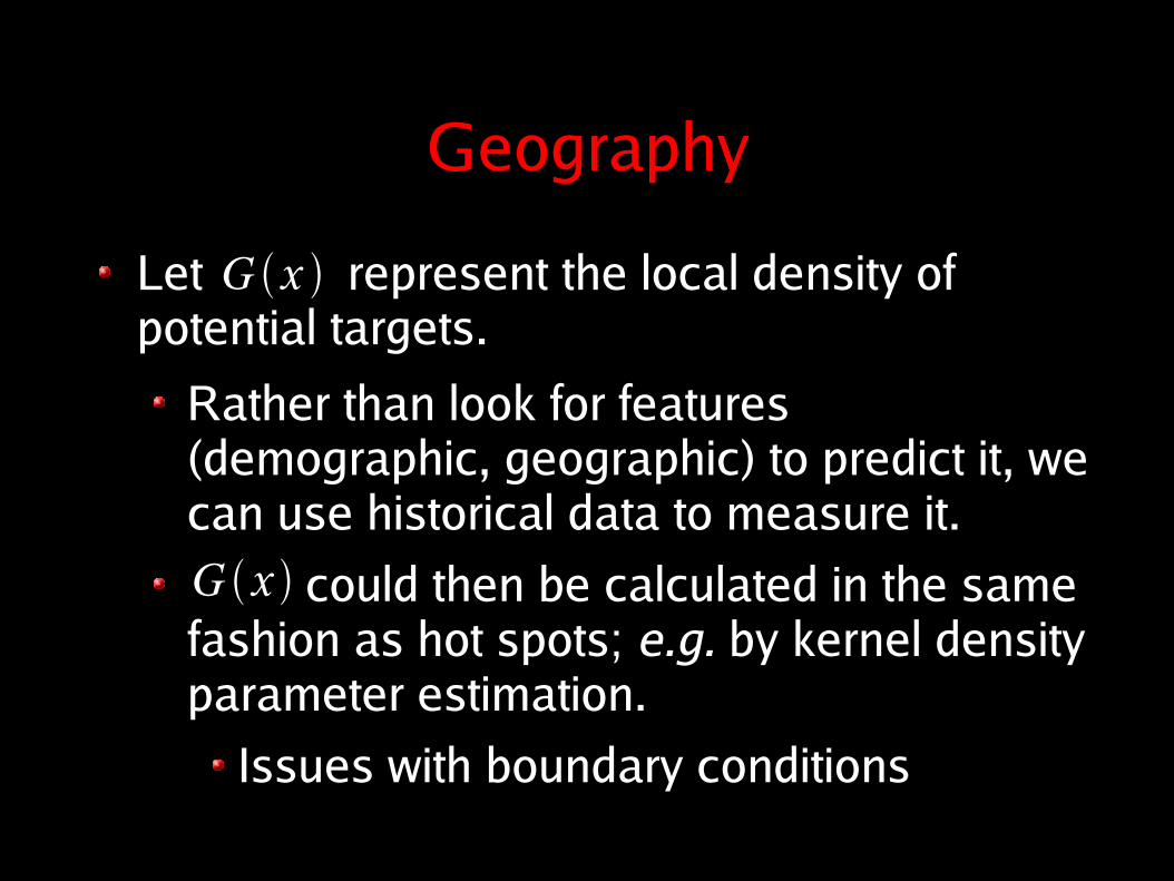
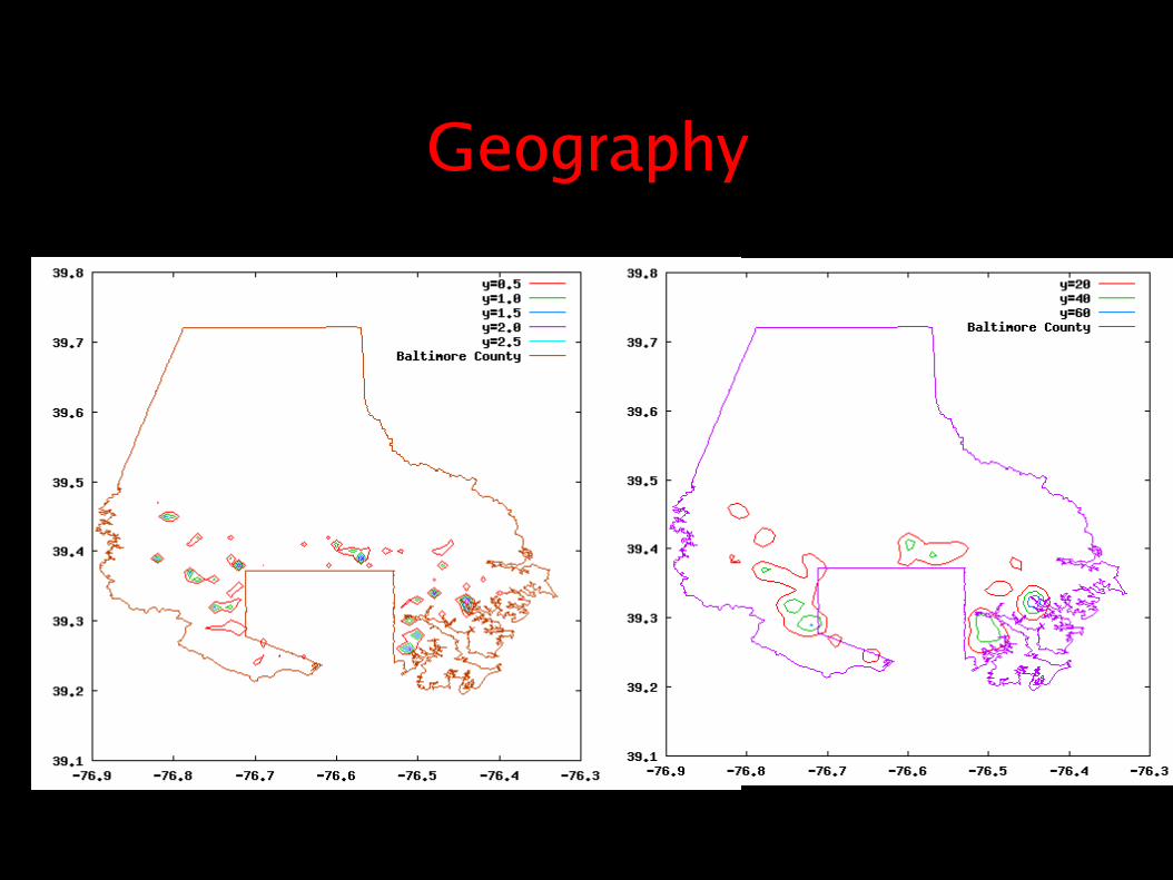
Let represent the local density of potential targets.

Rather than look for features (demographic, geographic) to predict it, we can use historical data to measure it.

could then be calculated in the same fashion as hot spots; e.g. by kernel density parameter estimation.

Issues with boundary conditions

G x

G x

Geography

Geography

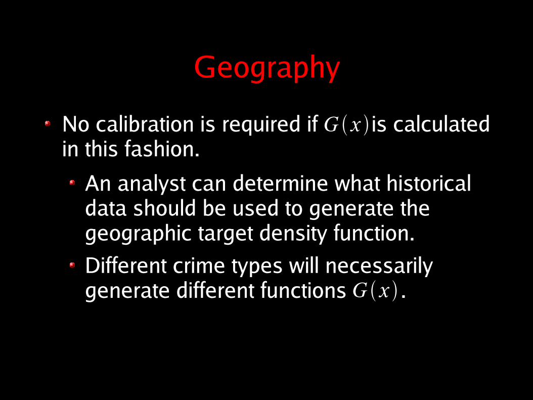
No calibration is required if is calculated in this fashion.

An analyst can determine what historical data should be used to generate the geographic target density function.

Different crime types will necessarily generate different functions .

G x

G x

Strengths of this Framework

All of the assumptions on criminal behavior are made in the open.

They can be challenged, tested, discussed and compared.

Strengths

The framework is extensible.

Vastly different situations can be modelled by making different choices for the form and structure of .

e.g. angular dependence, barriers.The framework is otherwise agnostic about the crime series; all of the relevant information must be encoded in .

P x ; z

P x ; z

Strengths

This framework is mathematically rigorous.

There are mathematical and criminological meanings to the maximum likelihood estimate .mle

Weaknesses of this Framework

GIGO

The method is only as accurate as the accuracy of the choice of .

It is unclear what the right choice is for

Even with the simplifying assumption that

this is difficult.

P x ; z P x ; z

P x ; z =D d x , z ⋅G x ⋅N z

Weaknesses

There is no simple closed mathematical form for .

Relatively complex techniques are required to estimate even for simple choices of .

The error analysis for maximum likelihood estimators is delicate when the number of data points is small.

mle

mle

P x ; z

Weaknesses

The framework assumes that crime sites are independent, identically distributed random variables.

This is probably false in general!

This should be a solvable problem though...

Weaknesses

We only produce the point estimate of .

Law enforcement agencies do not want “X Marks the Spot”.

A search area, rather than a point estimate is far preferable.

This should be possible with some Bayesian analysis

mle

Questions?

Contact information:

Dr. Mike O'Leary

Director, Applied Mathematics Laboratory

Towson University

Towson, MD 21252

410-704-7457

moleary@towson.edu