Embed Size (px)
Citation preview
Journal of Artificial Intelligence Research 22 (2004) 319-351 Submitted 12/03; published 12/04
Towards Understanding and Harnessing the
Potential of Clause Learning
Paul Beame [email protected]
Henry Kautz [email protected]
Ashish Sabharwal [email protected]
Computer Science and Engineering
University of Washington, Box 352350
Seattle, WA 98195-2350, USA
Abstract
Efficient implementations of DPLL with the addition of clause learning are the fastestcomplete Boolean satisfiability solvers and can handle many significant real-world prob-lems, such as verification, planning and design. Despite its importance, little is knownof the ultimate strengths and limitations of the technique. This paper presents the firstprecise characterization of clause learning as a proof system (CL), and begins the task ofunderstanding its power by relating it to the well-studied resolution proof system. In par-ticular, we show that with a new learning scheme, CL can provide exponentially shorterproofs than many proper refinements of general resolution (RES) satisfying a natural prop-erty. These include regular and Davis-Putnam resolution, which are already known to bemuch stronger than ordinary DPLL. We also show that a slight variant of CL with unlim-ited restarts is as powerful as RES itself. Translating these analytical results to practice,however, presents a challenge because of the nondeterministic nature of clause learningalgorithms. We propose a novel way of exploiting the underlying problem structure, in theform of a high level problem description such as a graph or PDDL specification, to guideclause learning algorithms toward faster solutions. We show that this leads to exponentialspeed-ups on grid and randomized pebbling problems, as well as substantial improvementson certain ordering formulas.
1. Introduction
In recent years the task of deciding whether or not a given CNF propositional logic formulais satisfiable has gone from a problem of theoretical interest to a practical approach forsolving real-world problems. Satisfiability (SAT) procedures are now a standard tool forhardware verification, including verification of super-scalar processors (Velev & Bryant,2001; Biere et al., 1999a). Open problems in group theory have been encoded and solvedusing satisfiability solvers (Zhang & Hsiang, 1994). Other applications of SAT includecircuit diagnosis and experiment design (Konuk & Larrabee, 1993; Gomes et al., 1998b).
The most surprising aspect of such relatively recent practical progress is that the bestcomplete satisfiability testing algorithms remain variants of the Davis-Putnam-Logemann-Loveland or DPLL procedure (Davis & Putnam, 1960; Davis et al., 1962) for backtracksearch in the space of partial truth assignments. The key idea behind its efficacy is thepruning of search space based on falsified clauses. Since its introduction in the early 1960’s,the main improvements to DPLL have been smart branch selection heuristics (e.g., Li &
c©2004 AI Access Foundation. All rights reserved.
Beame, Kautz, & Sabharwal
Anbulagan, 1997), and extensions such as randomized restarts (Gomes et al., 1998a) andclause learning (see e.g., Marques-Silva & Sakallah, 1996). One can argue that of these,clause learning has been the most significant in scaling DPLL to realistic problems. Thispaper attempts to understand the potential of clause learning and suggests ways to harnessits power.
Clause learning grew out of work in AI on explanation-based learning (EBL), whichsought to improve the performance of backtrack search algorithms by generating explana-tions for failure (backtrack) points, and then adding the explanations as new constraints onthe original problem (de Kleer & Williams, 1987; Stallman & Sussman, 1977; Genesereth,1984; Davis, 1984). For general constraint satisfaction problems the explanations are called“conflicts” or “no goods”; in the case of Boolean CNF satisfiability, the technique becomesclause learning – the reason for failure is learned in the form of a “conflict clause” whichis added to the set of given clauses. A series of researchers (Bayardo Jr. & Schrag, 1997;Marques-Silva & Sakallah, 1996; Zhang, 1997; Moskewicz et al., 2001; Zhang et al., 2001)showed that clause learning can be efficiently implemented and used to solve hard problemsthat cannot be approached by any other technique.
Despite its importance there has been little work on formal properties of clause learning,with the goal of understanding its fundamental strengths and limitations. A likely reasonfor such inattention is that clause learning is a rather complex rule of inference – in fact, aswe describe below, a complex family of rules of inference. A contribution of this paper is aprecise mathematical specification of various concepts used in describing clause learning.
Another problem in characterizing clause learning is defining a formal notion of thestrength or power of a reasoning method. This paper uses the notion of proof complex-ity (Cook & Reckhow, 1977), which compares inference systems in terms of the sizes ofthe shortest proofs they sanction. We use CL to denote clause learning viewed as a proofsystem. A family of formulas C provides an exponential separation between systems S1
and S2 if the shortest proofs of formulas in C in system S1 are exponentially smaller thanthe corresponding shortest proofs in S2. From this basic propositional proof complexitypoint of view, only families of unsatisfiable formulas are of interest, because only proofs ofunsatisfiability can be large; minimum proofs of satisfiability are linear in the number ofvariables of the formula. Nevertheless, Achlioptas et al. (2001) have shown how negativeproof complexity results for unsatisfiable formulas can be used to derive time lower boundsfor specific inference algorithms running on satisfiable formulas as well.
Proof complexity does not capture everything we intuitively mean by the power of areasoning system, because it says nothing about how difficult it is to find shortest proofs.However, it is a good notion with which to begin our analysis, because the size of proofsprovides a lower bound on the running time of any implementation of the system. In thesystems we consider, a branching function, which determines which variable to split uponor which pair of clauses to resolve, guides the search. A negative proof complexity resultfor a system tells us that a family of formulas is intractable even with a perfect branchingfunction; likewise, a positive result gives us hope of finding a branching function.
A basic result in proof complexity is that general resolution, denoted RES, is exponen-tially stronger than the DPLL procedure (Bonet et al., 2000; Ben-Sasson et al., 2000). Thisis because the trace of DPLL running on an unsatisfiable formula can be converted to a tree-like resolution proof of the same size, and tree-like proofs must sometimes be exponentially
320
Towards Understanding and Harnessing the Potential of Clause Learning
larger than the DAG-like proofs generated by RES. Although RES can yield shorter proofs,in practice DPLL is better because it provides a more efficient way to search for proofs.The weakness of the tree-like proofs that DPLL generates is that they do not reuse derivedclauses. The conflict clauses found when DPLL is augmented by clause learning correspondto reuse of derived clauses in the associated resolution proofs and thus to more general formsof resolution proofs. As a theoretical upper bound, all DPLL based approaches, includingthose involving clause learning, are captured by RES. An intuition behind the results in thispaper is that the addition of clause learning moves DPLL closer to RES while retaining itspractical efficiency.
It has been previously observed that clause learning can be viewed as adding resolvents toa tree-like proof (Marques-Silva, 1998). However, this paper provides the first mathematicalproof that clause learning, viewed as a propositional proof system CL, is exponentiallystronger than tree-like resolution. This explains, formally, the performance gains observedempirically when clause learning is added to DPLL based solvers. Further, we describe ageneric way of extending families of formulas to obtain ones that exponentially separateCL from many refinements of resolution known to be intermediate in strength between RES
and tree-like resolution. These include regular and Davis-Putnam resolution, and any otherproper refinement of RES that behaves naturally under restrictions of variables, i.e., for anyformula F and restriction ρ on its variables, the shortest proof of F |ρ in the system is notany larger than a proof of F itself. The argument used to prove this result involves a newclause learning scheme called FirstNewCut that we introduce specifically for this purpose.Our second technical result shows that combining a slight variant of CL, denoted CL--, withunlimited restarts results in a proof system as strong as RES itself. This intuitively explainsthe speed-ups obtained empirically when randomized restarts are added to DPLL basedsolvers, with or without clause learning.
Given these results about the strengths and limitations of clause learning, it is naturalto ask how the understanding we gain through this kind of analysis may lead to practicalimprovement in SAT solvers. The theoretical bounds tell us the potential power of clauselearning; they don’t give us a way of finding short solutions when they exist. In order toleverage their strength, clause learning algorithms must follow the “right” variable order fortheir branching decisions for the underlying DPLL procedure. While a good variable ordermay result in a polynomial time solution, a bad one can make the process as slow as basicDPLL without learning. The latter half of this paper addresses this problem of moving fromanalytical results to practical improvement. The approach we take is the use of the problemstructure for guiding SAT solvers in their branch decisions.
Both random CNF formulas and those encoding various real-world problems are quitehard for current SAT solvers. However, while DPLL based algorithms with lookahead butno learning (such as satz by Li & Anbulagan, 1997) and those that try only one carefullychosen assignment without any backtracks (such as SurveyProp by Mezard & Zecchina,2002) are our best tools for solving random formula instances, formulas arising from variousreal applications seem to require clause learning as a critical ingredient. The key thing thatmakes this second class of formulas different is the inherent structure, such as dependencegraphs in scheduling problems, causes and effects in planning, and algebraic structure ingroup theory.
321
Beame, Kautz, & Sabharwal
Most theoretical and practical problem instances of satisfiability problems originate, notsurprisingly, from a higher level description, such as planning domain definition language orPDDL specification for planning, timed automata or logic description for model checking,task dependency graph for scheduling, circuit description for VLSI, algebraic structure forgroup theory, and processor specification for hardware. Typically, this description containsmore structure of the original problem than is visible in the flat CNF representation inDIMACS format (Johnson & Trick, 1996) to which it is converted before being fed intoa SAT solver. This structure can potentially be used to gain efficiency in the solutionprocess. While there has been work on extracting structure after conversion into a CNFformula by exploiting variable dependency (Giunchiglia et al., 2002; Ostrowski et al., 2002),constraint redundancy (Ostrowski et al., 2002), symmetry (Aloul et al., 2002), binary clauses(Brafman, 2001), and partitioning (Amir & McIlraith, 2000), using the original higher leveldescription itself to generate structural information is likely to be more effective. The latterapproach, despite its intuitive appeal, remains largely unexplored, except for suggested usein bounded model checking (Shtrichman, 2000) and the separate consideration of causevariables and effect variables in planning (Kautz & Selman, 1996).
In this paper, we further open this line of research by proposing an effective methodfor exploiting problem structure to guide the branching decision process of clause learningalgorithms. Our approach uses the original high level problem description to generate notonly a CNF encoding but also a branching sequence that guides the SAT solver toward anefficient solution. This branching sequence serves as auxiliary structural information thatwas possibly lost in the process of encoding the problem as a CNF formula. It makes clauselearning algorithms learn useful clauses instead of wasting time learning those that may notbe reused in future at all. We give an exact sequence generation algorithm for pebblingformulas, using the underlying pebbling graph as the high level description. We also give amuch simpler but approximate branching sequence generation algorithm for GTn formulas,utilizing their underlying ordering structure. Our sequence generators work for the 1UIPlearning scheme (Zhang et al., 2001), which is one of the best known. They can also beextended to other schemes, including FirstNewCut. Our empirical results are based on ourextension of the popular SAT solver zChaff (Moskewicz et al., 2001).
We show that the use of branching sequences produced by our generator leads to expo-nential empirical speedups for the class of grid and randomized pebbling formulas. Theseformulas, more commonly occurring in theoretical proof complexity literature (Ben-Sassonet al., 2000; Beame et al., 2003a), can be thought of as representing precedence graphs independent task systems and scheduling scenarios. They can also be viewed as restrictedplanning problems. Although admitting a polynomial size solution, both grid and random-ized pebbling problems are not so easy to solve deterministically, as is indicated by ourexperimental results for unmodified zChaff. We also report significant gains obtained forthe class of GTn formulas which, again, have appeared frequently in proof complexity results(Krishnamurthy, 1985; Bonet & Galesi, 2001; Alekhnovich et al., 2002). From a broaderperspective, our results for pebbling and GTn formulas serve as a proof of concept thatanalysis of problem structure can be used to achieve dramatic improvements even in thecurrent best clause learning based SAT solvers.
322
Towards Understanding and Harnessing the Potential of Clause Learning
2. Preliminaries
A CNF formula F is an and (∧) of clauses, where each clause is an or (∨) of literals, anda literal is a variable or its negation (¬). It is natural to think of F as a set of clauses andeach clause as a set of literals. A clause that is a subset of another is called its subclause.The size of F is the number of clauses in F .
Let ρ be a partial assignment to the variables of F . The restricted formula F ρ is obtainedfrom F by replacing variables in ρ with their assigned values. F is said to be simplified ifall clauses with at least one true literal are deleted and all occurrences of false literalsare removed from clauses. F |ρ denotes the result of simplifying the restricted formula F ρ.
2.1 The DPLL Procedure
The basic idea of the Davis-Putnam-Logemann-Loveland (DPLL) procedure (Davis & Put-nam, 1960; Davis et al., 1962) for testing satisfiability of CNF formulas is to branch onvariables, setting them to true or false, until either an initial clause is violated (i.e. hasall literals set to false) or no more clauses remain in the simplified residual formula. In theformer case, we backtrack to the last branching decision whose other branch has not beentried yet, reverse the decision, and proceed recursively. In the latter, we terminate with asatisfying assignment. If all possible branches have been unsuccessfully tried, the formula isdeclared unsatisfiable. To increase efficiency, unit clauses (those with only one unset literal)are immediately set to true. Pure literals (those whose negation does not appear) are alsoset to true as a preprocessing step and, in some implementations, in the simplificationprocess after every branch.
In this paper, we will use the term DPLL to denote the basic branching and backtrackingprocedure described above. It will not include learning conflict clauses when backtracking,but will allow intelligent branching heuristics as well as common extensions such as fastbacktracking and restarts. Note that this is in contrast with the occasional use of the termDPLL to encompass practically all branching and backtracking approaches to SAT, includingthose involving learning.
2.2 Proof Systems
A propositional proof system (Cook & Reckhow, 1977) is a polynomial time computablepredicate S such that a propositional formula F is unsatisfiable iff there exists a proof p forwhich S(F, p) holds. In other words, it is an efficient (in the size of the proof) procedure tocheck the correctness of proofs presented in a certain format. Finding short proofs, however,may still be difficult. In fact, short proofs may not exist in the proof system if it is tooweak. In the rest of this paper, we refer to such systems simply as proof systems and omitthe word propositional.
Definition 1. For a proof system S and an unsatisfiable formula F , the complexity of Fin S, denoted CS(F ), is the length of the shortest refutation of F in S. For a family Fnof formulas over increasing number of variables n, its asymptotic complexity in S, denotedCS(Fn) with abuse of notation, is measured with respect to the increasing sizes of Fn.
Definition 2. For proof systems S and T , and a function f : N→ N,
323
Beame, Kautz, & Sabharwal
• S is natural if for any formula F and restriction ρ on its variables, CS(F |ρ) ≤ CS(F ).
• S is a refinement of T if proofs in S are also (restricted) proofs in T .
• A refinement S of T is f(n)-proper if there exists a witnessing family Fn of formulassuch that CS(Fn) ≥ f(n) · CT (Fn). The refinement is exponentially-proper if f(n) =
2nΩ(1)and super-polynomially-proper if f(n) = nω(1).
2.3 Resolution
Resolution (RES) is a widely studied simple proof system that can be used to prove unsat-isfiability of CNF formulas. Our complexity results concerning the power of clause learningare in relation to this system. The resolution rule states that given clauses (A ∨ x) and(B∨¬x), we can derive clause (A∨B) by resolving on x. A resolution derivation of C froma CNF formula F is a sequence π = (C1, C2, . . . , Cs ≡ C) where each clause Ci is eithera clause of F (an initial clause) or derived by applying the resolution rule to Cj and Ck,j, k < i (a derived clause). The size of π is s, the number of clauses occurring in it. We willassume that each Cj 6= C in π is used to derive at least one other clause Ci, i > j. Anyderivation of the empty clause Λ from F , also called a refutation or proof of F , shows thatF is unsatisfiable.
Despite its simplicity, unrestricted resolution is hard to implement efficiently due to thedifficulty of finding good choices of clauses to resolve; natural choices typically yield hugestorage requirements. Various restrictions on the structure of resolution proofs lead to lesspowerful but easier to implement refinements that have been studied well, such as tree-like, regular, linear, positive, negative, semantic, and Davis-Putnam resolution. Tree-likeresolution uses non-empty derived clauses exactly once in the proof and is equivalent to anoptimal DPLL procedure. Regular resolution allows any variable to be resolved upon at mostonce along any “path” in the proof from an initial clause to Λ, allowing (restricted) reuseof derived clauses. Linear resolution requires each clause Ci in a derivation (C1, C2, . . . , Cs)to be either an initial clause or be derived by resolving Ci−1 with Cj , j < i − 1. For anyassignment α to the variables, an α-derivation requires at least one clause involved in eachresolution step to be falsified by α. When α is the all false assignment, the derivation ispositive. When it is the all true assignment, the derivation is negative. A derivation issemantic if it is an α-derivation for some α. Davis-Putnam resolution, also called orderedresolution, is a refinement of regular resolution where every sequence of variables in a pathfrom an initial clause to Λ respects the same ordering on the variables.
While all these refinements are sound and complete as proof systems, they differ inefficiency. For instance, regular, linear, positive, negative, semantic, and Davis-Putnamresolution are all known to be exponentially stronger than tree-like resolution (Bonet et al.,2000; Bonet & Galesi, 2001; Buresh-Oppenheim & Pitassi, 2003) whereas tree-like, regular,and Davis-Putnam resolution are known to be exponentially weaker than RES (Bonet et al.,2000; Alekhnovich et al., 2002).
Proposition 1. Tree-like, regular, linear, positive, negative, semantic, and Davis-Putnamresolution are natural refinements of RES.
Proposition 2 (Bonet et al., 2000; Alekhnovich et al., 2002). Tree-like, regular, andDavis-Putnam resolution are exponentially-proper natural refinements of RES.
324
Towards Understanding and Harnessing the Potential of Clause Learning
2.4 Clause Learning
Clause learning (see e.g., Marques-Silva & Sakallah, 1996) can be thought of as an exten-sion of the DPLL procedure that caches causes of assignment failures in the form of learnedclauses. It proceeds by following the normal branching process of DPLL until there is a “con-flict” after unit propagation. If this conflict occurs when no variable is currently branchedupon, the formula is declared unsatisfiable. Otherwise, the “conflict graph” is analyzed andthe “cause” of the conflict is learned in the form of a “conflict clause.” The procedure nowbacktracks and continues as in ordinary DPLL, treating the learned clause just like initialones. A clause is said to be known at a stage if it is either an initial clause or has previouslybeen learned.
The learning process is expected to save us from redoing the same computation when welater have an assignment that causes conflict due in part to the same reason. Variations ofsuch conflict-driven learning include different ways of choosing the clause to learn (differentlearning schemes) and possibly allowing multiple clauses to be learned from a single conflict(Zhang et al., 2001). In the last decade, many algorithms based on this idea have beenproposed and demonstrated to be empirically successful on large problems that could not behandled using other methodologies (Bayardo Jr. & Schrag, 1997; Marques-Silva & Sakallah,1996; Zhang, 1997; Moskewicz et al., 2001). We leave a more detailed discussion of theconcepts involved in clause learning as well as its formulation as a proof system CL toSection 3.
2.5 Pebbling Formulas
Pebbling formulas are unsatisfiable CNF formulas whose variations have been used repeat-edly in proof complexity to obtain theoretical separation results between different proofsystems (Ben-Sasson et al., 2000; Beame et al., 2003a). The version we will use in thispaper is known to be easy for regular resolution but hard for tree-like resolution, and hencefor DPLL without learning (Ben-Sasson et al., 2000). We use these formulas to show howone can utilize problem structure to allow clause learning algorithms to handle much biggerproblems than they otherwise can.
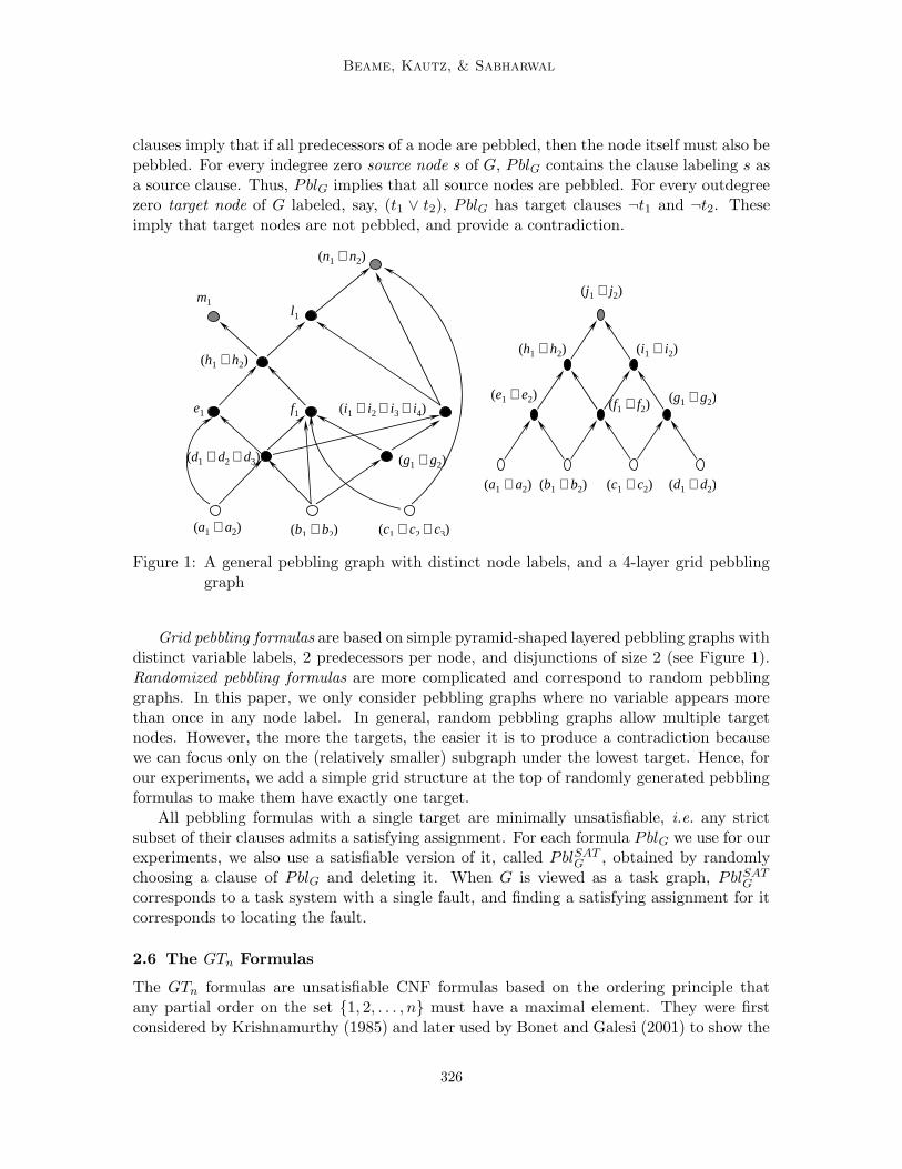
Pebbling formulas represent the constraints for sequencing a system of tasks that needto be completed, where each task can be accomplished in a number of alternative ways. Theassociated pebbling graph has a node for each task, labeled by a disjunction of variablesrepresenting the different ways of completing the task. Placing a pebble on a node inthe graph represents accomplishing the corresponding task. Directed edges between nodesdenote task precedence; a node is pebbled when all of its predecessors in the graph arepebbled. The pebbling process is initialized by placing pebbles on all indegree zero nodes.This corresponds to completing those tasks that do not depend on any other.
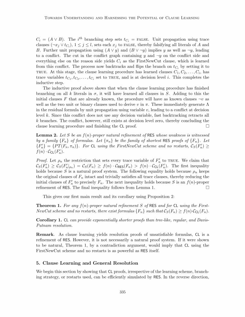
Formally, a Pebbling formula PblG is an unsatisfiable CNF formula associated with adirected, acyclic pebbling graph G (see Figure 1). Nodes of G are labeled with disjunctionsof variables, i.e. with clauses. A node labeled with clause C is thought of as pebbled undera (partial) variable assignment σ if C|σ = true. PblG contains three kinds of clauses –precedence clauses, source clauses and target clauses. For instance, a node labeled (x1∨x2)with three predecessors labeled (p1∨p2∨p3), q1 and (r1∨r2) generates six precedence clauses(¬pi ∨ ¬qj ∨ ¬rk ∨ x1 ∨ x2), where i ∈ 1, 2, 3, j ∈ 1 and k ∈ 1, 2. The precedence
325
Beame, Kautz, & Sabharwal
clauses imply that if all predecessors of a node are pebbled, then the node itself must also bepebbled. For every indegree zero source node s of G, PblG contains the clause labeling s asa source clause. Thus, PblG implies that all source nodes are pebbled. For every outdegreezero target node of G labeled, say, (t1 ∨ t2), PblG has target clauses ¬t1 and ¬t2. Theseimply that target nodes are not pebbled, and provide a contradiction.
(a1 ∨ a2) (c1 ∨ c2 ∨ c3)
(d1 ∨ d2 ∨ d3)
l1
(h1 ∨ h2)
(i1 ∨ i2 ∨ i3 ∨ i4)e1
(g1 ∨ g2)
f1
(n1 ∨ n2)
m1(j1 ∨ j2)
(h1 ∨ h2) (i1 ∨ i2)
(f1 ∨ f2)(g1 ∨ g2)
(d1 ∨ d2)(c1 ∨ c2)(b1 ∨ b2)(a1 ∨ a2)
(e1 ∨ e2)
(b1 ∨ b2)
Figure 1: A general pebbling graph with distinct node labels, and a 4-layer grid pebblinggraph
Grid pebbling formulas are based on simple pyramid-shaped layered pebbling graphs withdistinct variable labels, 2 predecessors per node, and disjunctions of size 2 (see Figure 1).Randomized pebbling formulas are more complicated and correspond to random pebblinggraphs. In this paper, we only consider pebbling graphs where no variable appears morethan once in any node label. In general, random pebbling graphs allow multiple targetnodes. However, the more the targets, the easier it is to produce a contradiction becausewe can focus only on the (relatively smaller) subgraph under the lowest target. Hence, forour experiments, we add a simple grid structure at the top of randomly generated pebblingformulas to make them have exactly one target.
All pebbling formulas with a single target are minimally unsatisfiable, i.e. any strictsubset of their clauses admits a satisfying assignment. For each formula PblG we use for ourexperiments, we also use a satisfiable version of it, called PblSAT
G , obtained by randomlychoosing a clause of PblG and deleting it. When G is viewed as a task graph, PblSAT
G
corresponds to a task system with a single fault, and finding a satisfying assignment for itcorresponds to locating the fault.
2.6 The GTn Formulas
The GTn formulas are unsatisfiable CNF formulas based on the ordering principle thatany partial order on the set 1, 2, . . . , n must have a maximal element. They were firstconsidered by Krishnamurthy (1985) and later used by Bonet and Galesi (2001) to show the
326
Towards Understanding and Harnessing the Potential of Clause Learning
optimality of the size-width relationship of resolution proofs. Recently, Alekhnovich et al.(2002) used a variation, called GT ′
n, to show an exponential separation between RES andregular resolution.
The variables of GTn are xi,j for i, j ∈ [n], i 6= j, which should be thought of as thebinary predicate i j. Clauses (¬xi,j ∨¬xj,i) ensure that is anti-symmetric and (¬xi,j ∨¬xj,k ∨ xi,k) ensure that is transitive. This makes a partial order on [n]. Successorclauses (∨k 6=jxk,j) provide the contradiction by saying that every element j has a successorin [n] \ j, which is clearly false for the maximal elements of [n] under the ordering .
These formulas, although capturing a simple mathematical principle, are empiricallydifficult for many SAT solvers including zChaff. We employ our techniques to improve theperformance of zChaff on these formulas. We use for our experiments the unsatisfiableversion GTn described above as well as a satisfiable version GT SAT
n obtained by deletinga randomly chosen successor clause. The reason we consider these ordering formulas inaddition to seemingly harder pebbling formulas is that the latter admit short tree-likeproofs in certain extensions of RES whereas the former seem to critically require reuse ofderived or learned clauses for short refutations. We elaborate on this in Section 6.2.
3. A Formal Framework for Studying Clause Learning
Although many SAT solvers based on clause learning have been proposed and demonstratedto be empirically successful, a theoretical discussion of the underlying concepts and struc-tures needed for our analysis is lacking. This section focuses on this formal framework.
3.1 Unit Propagation and Decision Levels
All clause learning algorithms discussed in this paper are based on unit propagation, whichis the process of repeatedly applying the unit clause rule followed by formula simplificationuntil no clause with exactly one unassigned literal remains. In this context, it is convenientto work with residual formulas at different stages of DPLL. Let ρ be the partial assignmentat some stage of DPLL on formula F . The residual formula at this stage is obtained byapplying unit propagation to the simplified formula F |ρ.
When using unit propagation, variables assigned values through the actual branchingprocess are called decision variables and those assigned values as a result of unit propagationare called implied variables. Decision and implied literals are analogously defined. Uponbacktracking, the last decision variable no longer remains a decision variable and mightinstead become an implied variable depending on the clauses learned so far. The decisionlevel of a decision variable x is one more than the number of current decision variables atthe time of branching on x. The decision level of an implied variable is the maximum ofthe decision levels of decision variables used to imply it. The decision level at any step ofthe underlying DPLL procedure is the maximum of the decision levels of all current decisionvariables. Thus, for instance, if the clause learning algorithm starts off by branching on x,the decision level of x is 1 and the algorithm at this stage is at decision level 1.
A clause learning algorithm stops and declares the given formula to be unsatisfiablewhenever unit propagation leads to a conflict at decision level zero, i.e. when no variableis currently branched upon. This condition will be referred to in this paper as a conflict atdecision level zero.
327
Beame, Kautz, & Sabharwal
3.2 Branching Sequence
We use the notion of branching sequence to prove an exponential separation between DPLL
and clause learning. It generalizes the idea of a static variable order by letting the orderdiffer from branch to branch in the underlying DPLL procedure. In addition, it also specifieswhich branch (true or false) to explore first. This can clearly be useful for satisfiableformulas, and can also help on unsatisfiable ones by making the algorithm learn usefulclauses earlier in the process.
Definition 3. A branching sequence for a CNF formula F is a sequence σ = (l1, l2, . . . , lk) ofliterals of F , possibly with repetitions. A DPLL based algorithm A on F branches accordingto σ if it always picks the next variable v to branch on in the literal order given by σ, skipsv if v is currently assigned a value, and otherwise branches further by setting the chosenliteral to false and deleting it from σ. When σ becomes empty, A reverts back to itsdefault branching scheme.
Definition 4. A branching sequence σ is complete for a formula F under a DPLL basedalgorithm A if A branching according to σ terminates before or as soon as σ becomes empty.Otherwise it is incomplete or approximate.
Clearly, how well a branching sequence works for a formula depends on the specifics ofthe clause learning algorithm used, such as its learning scheme and backtracking process.One needs to keep these in mind when generating the sequence. It is also important to notethat while the size of a variable order is always the same as the number of variables in theformula, that of an effective branching sequence is typically much more. In fact, the sizeof a branching sequence complete for an unsatisfiable formula F is equal to the size of anunsatisfiability proof of F , and when F is satisfiable, it is proportional to the time neededto find a satisfying assignment.
3.3 Clause Learning Proofs
The notion of clause learning proofs connects clause learning with resolution and providesthe basis for our complexity bounds. If a given CNF formula F is unsatisfiable, clauselearning terminates with a conflict at decision level zero. Since all clauses used in thisfinal conflict themselves follow directly or indirectly from F , this failure of clause learningin finding a satisfying assignment constitutes a logical proof of unsatisfiability of F . Wedenote by CL the proof system consisting of all such proofs. Our bounds compare the sizesof proofs in CL with the sizes of (possibly restricted) resolution proofs. Recall that clauselearning algorithms can use one of many learning schemes, resulting in different proofs.
Definition 5. A clause learning (CL) proof π of an unsatisfiable CNF formula F underlearning scheme S and induced by branching sequence σ is the result of applying DPLL
with unit propagation on F , branching according to σ, and using scheme S to learn conflictclauses such that at the end of this process, there is a conflict at decision level zero. Thesize of the proof, size(π), is |σ|.
328
Towards Understanding and Harnessing the Potential of Clause Learning
3.4 Implication Graph and Conflicts
Unit propagation can be naturally associated with an implication graph that captures allpossible ways of deriving all implied literals from decision literals.
Definition 6. The implication graph G at a given stage of DPLL is a directed acyclic graphwith edges labeled with sets of clauses. It is constructed as follows:
1. Create a node for each decision literal, labeled with that literal. These will be theindegree zero source nodes of G.
2. While there exists a known clause C = (l1 ∨ . . . lk ∨ l) such that ¬l1, . . . ,¬lk labelnodes in G,
(a) Add a node labeled l if not already present in G.
(b) Add edges (li, l), 1 ≤ i ≤ k, if not already present.
(c) Add C to the label set of these edges. These edges are thought of as groupedtogether and associated with clause C.
3. Add to G a special node Λ. For any variable x which occurs both positively andnegatively in G, add directed edges from x and ¬x to Λ.
Since all node labels in G are distinct, we identify nodes with the literals labeling them.Any variable x occurring both positively and negatively in G is a conflict variable, and x aswell as ¬x are conflict literals. G contains a conflict if it has at least one conflict variable.DPLL at a given stage has a conflict if the implication graph at that stage contains a conflict.A conflict can equivalently be thought of as occurring when the residual formula containsthe empty clause Λ.
By definition, an implication graph may not contain a conflict at all, or it may containmany conflict variables and several ways of deriving any single literal. To better understandand analyze a conflict when it occurs, we work with a subgraph of an implication graph,called the conflict graph (see Figure 2), that captures only one among possibly many waysof reaching a conflict from the decision variables using unit propagation.
Definition 7. A conflict graph H is any subgraph of an implication graph with the followingproperties:
1. H contains Λ and exactly one conflict variable.
2. All nodes in H have a path to Λ.
3. Every node l in H other than Λ either corresponds to a decision literal or has preciselythe nodes ¬l1,¬l2, . . . ,¬lk as predecessors where (l1∨ l2∨ . . .∨ lk∨ l) is a known clause.
While an implication graph may or may not contain conflicts, a conflict graph alwayscontains exactly one. The choice of the conflict graph is part of the strategy of the solver.A typical strategy will maintain one subgraph of an implication graph that has properties2 and 3 from Definition 7, but not property 1. This can be thought of as a unique inferencesubgraph of the implication graph. When a conflict is reached, this unique inference sub-graph is extended to satisfy property 1 as well, resulting in a conflict graph, which is thenused to analyze the conflict.
329
Beame, Kautz, & Sabharwal
FirstNewCut clause(x1 ∨ x2 ∨ x3)
Decision clause(p ∨ q ∨ ¬ b)
1UIP clauset
rel-sat clause(¬ a ∨ ¬ b)
¬ p
¬ q
b
a
¬ t
¬ x1
¬ x2
¬ x3
y
¬¬¬¬ y
Λ
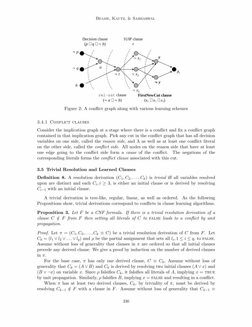
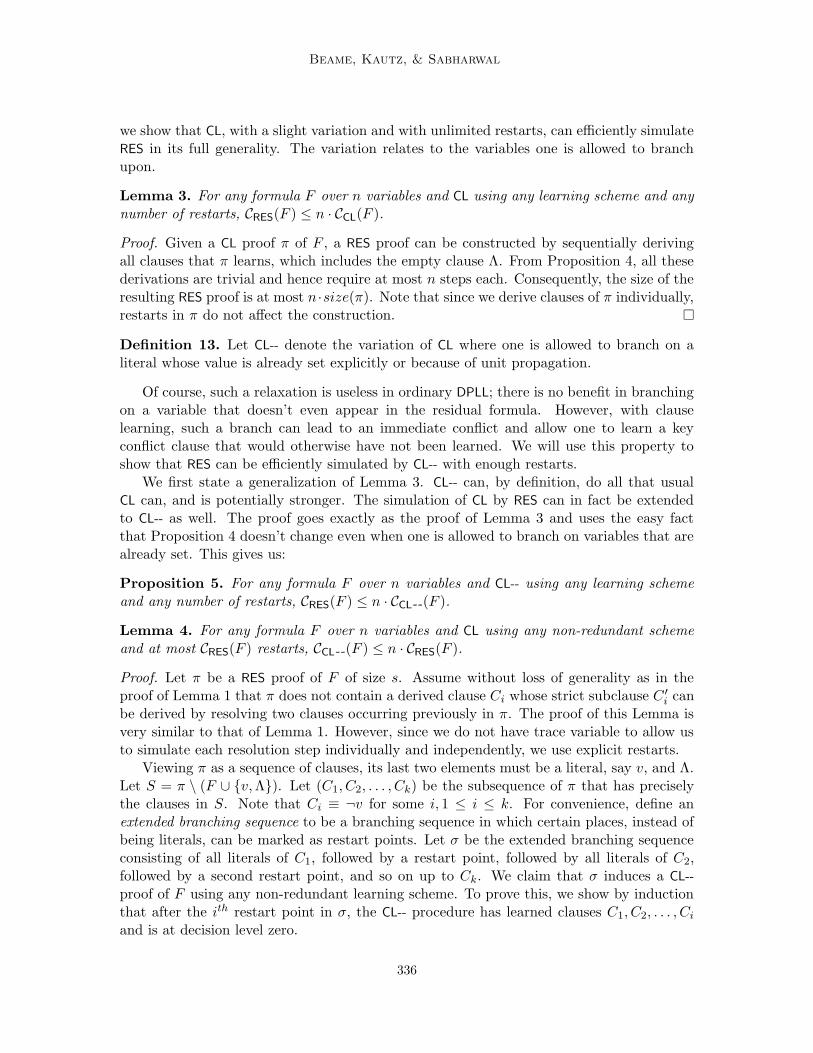
Figure 2: A conflict graph along with various learning schemes
3.4.1 Conflict clauses
Consider the implication graph at a stage where there is a conflict and fix a conflict graphcontained in that implication graph. Pick any cut in the conflict graph that has all decisionvariables on one side, called the reason side, and Λ as well as at least one conflict literalon the other side, called the conflict side. All nodes on the reason side that have at leastone edge going to the conflict side form a cause of the conflict. The negations of thecorresponding literals forms the conflict clause associated with this cut.
3.5 Trivial Resolution and Learned Clauses
Definition 8. A resolution derivation (C1, C2, . . . , Ck) is trivial iff all variables resolvedupon are distinct and each Ci, i ≥ 3, is either an initial clause or is derived by resolvingCi−1 with an initial clause.
A trivial derivation is tree-like, regular, linear, as well as ordered. As the followingPropositions show, trivial derivations correspond to conflicts in clause learning algorithms.
Proposition 3. Let F be a CNF formula. If there is a trivial resolution derivation of aclause C /∈ F from F then setting all literals of C to false leads to a conflict by unitpropagation.
Proof. Let π = (C1, C2, . . . , Ck ≡ C) be a trivial resolution derivation of C from F . LetCk = (l1 ∨ l2 ∨ . . . ∨ lq) and ρ be the partial assignment that sets all li, 1 ≤ i ≤ q, to false.Assume without loss of generality that clauses in π are ordered so that all initial clausesprecede any derived clause. We give a proof by induction on the number of derived clausesin π.
For the base case, π has only one derived clause, C ≡ Ck, Assume without loss ofgenerality that Ck = (A∨B) and Ck is derived by resolving two initial clauses (A∨ x) and(B ∨ ¬x) on variable x. Since ρ falsifies Ck, it falsifies all literals of A, implying x = true
by unit propagation. Similarly, ρ falsifies B, implying x = false and resulting in a conflict.When π has at least two derived clauses, Ck, by triviality of π, must be derived by
resolving Ck−1 /∈ F with a clause in F . Assume without loss of generality that Ck−1 ≡
330
Towards Understanding and Harnessing the Potential of Clause Learning
(A∨x) and the clause from F used in this resolution step is (B ∨¬x), where Ck = (A∨B).Since ρ falsifies C ≡ Ck, it falsifies all literals of B, implying x = false by unit propagation.This in turn results in falsifying all literals of Ck−1 because all literals of A are also set tofalse by ρ. Now (C1, . . . , Ck−1) is a trivial resolution derivation of Ck−1 /∈ F from F withone less derived clause than π, and all literals of Ck−1 are falsified. By induction, this mustlead to a conflict by unit propagation.
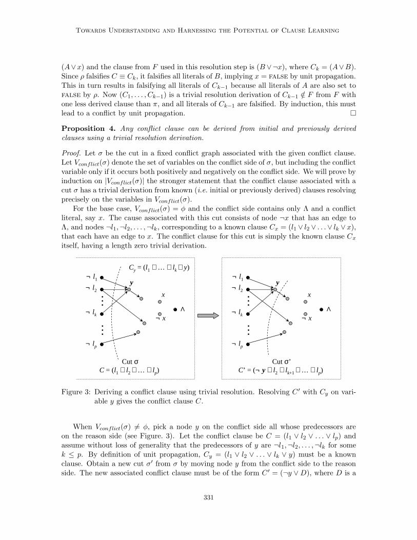
Proposition 4. Any conflict clause can be derived from initial and previously derivedclauses using a trivial resolution derivation.
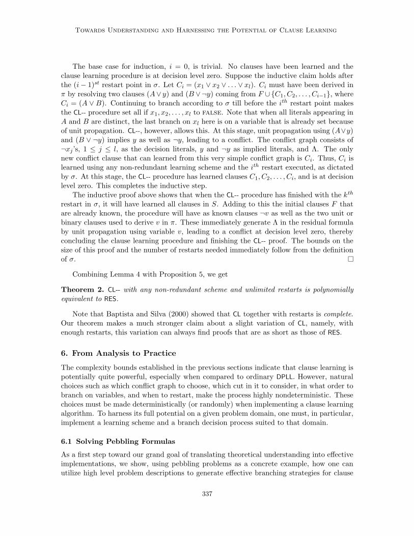
Proof. Let σ be the cut in a fixed conflict graph associated with the given conflict clause.Let Vconflict(σ) denote the set of variables on the conflict side of σ, but including the conflictvariable only if it occurs both positively and negatively on the conflict side. We will prove byinduction on |Vconflict(σ)| the stronger statement that the conflict clause associated with acut σ has a trivial derivation from known (i.e. initial or previously derived) clauses resolvingprecisely on the variables in Vconflict(σ).
For the base case, Vconflict(σ) = φ and the conflict side contains only Λ and a conflictliteral, say x. The cause associated with this cut consists of node ¬x that has an edge toΛ, and nodes ¬l1,¬l2, . . . ,¬lk, corresponding to a known clause Cx = (l1 ∨ l2 ∨ . . .∨ lk ∨ x),that each have an edge to x. The conflict clause for this cut is simply the known clause Cx
itself, having a length zero trivial derivation.
¬ l1¬ l2
y
……
¬ lk
¬ lp
¬ x
x
Λ
Cut σC = (l1 ∨ l2 ∨ … ∨ lp)
¬ l1¬ l2
y
……
¬ lk
¬ lp
¬ x
x
Λ
Cut σ’C’ = (¬ y ∨ l2 ∨ lk+1 ∨ … ∨ lp)
Cy = (l1 ∨ … ∨ lk ∨ y)
Figure 3: Deriving a conflict clause using trivial resolution. Resolving C ′ with Cy on vari-able y gives the conflict clause C.
When Vconflict(σ) 6= φ, pick a node y on the conflict side all whose predecessors areon the reason side (see Figure. 3). Let the conflict clause be C = (l1 ∨ l2 ∨ . . . ∨ lp) andassume without loss of generality that the predecessors of y are ¬l1,¬l2, . . . ,¬lk for somek ≤ p. By definition of unit propagation, Cy = (l1 ∨ l2 ∨ . . . ∨ lk ∨ y) must be a knownclause. Obtain a new cut σ′ from σ by moving node y from the conflict side to the reasonside. The new associated conflict clause must be of the form C ′ = (¬y ∨D), where D is a
331
Beame, Kautz, & Sabharwal
subclause of C. Now Vconflict(σ′) ⊂ Vconflict(σ). Consequently, by induction, C ′ must have
a trivial resolution derivation from known clauses resolving precisely upon the variables inVconflict(σ
′). Recall that no variable occurs twice in a conflict graph except the conflictvariable. Hence Vconflict(σ
′) has exactly all variables of Vconflict(σ) other than y. Using thistrivial derivation of C ′ and finally resolving C ′ with the known clause Cy on variable y givesus a trivial derivation of C from known clauses. This completes the inductive step.
3.6 Different Learning Schemes
Different cuts separating decision variables from Λ and a conflict literal correspond to differ-ent learning schemes (see Figure 2). One can also create learning schemes based on cuts notinvolving conflict literals at all (Zhang et al., 2001), but the effectiveness of such schemesis not clear. These will not be considered here.
It is insightful to think of the nondeterministic scheme as the most general learningscheme. Here we pick the cut nondeterministically, choosing, whenever possible, one whoseassociated clause is not already known. Since we can repeatedly branch on the same lastvariable, nondeterministic learning subsumes learning multiple clauses from a single conflictas long as the sets of nodes on the reason side of the corresponding cuts form a (set-wise)decreasing sequence. For simplicity, we will assume that only one clause is learned fromany conflict.
In practice, however, we employ deterministic schemes. The decision scheme (Zhanget al., 2001), for example, uses the cut whose reason side comprises all decision variables.rel-sat (Bayardo Jr. & Schrag, 1997) uses the cut whose conflict side consists of all impliedvariables at the current decision level. This scheme allows the conflict clause to have exactlyone variable from the current decision level, causing an automatic flip in its assignment uponbacktracking.
This nice flipping property holds in general for all unique implication points (UIPs)(Marques-Silva & Sakallah, 1996). A UIP of an implication graph is a node at the currentdecision level d such that any path from the decision variable at level d to the conflictvariable as well as its negation must go through it. Intuitively, it is a single reason at leveld that causes the conflict. Whereas rel-sat uses the decision variable as the obvious UIP,GRASP (Marques-Silva & Sakallah, 1996) and zChaff (Moskewicz et al., 2001) use FirstUIP,the one that is “closest” to the conflict variable. GRASP also learns multiple clauses whenfaced with a conflict. This makes it typically require fewer branching steps but possiblyslower because of the time lost in learning and unit propagation.
The concept of UIP can be generalized to decision levels other than the current one.The 1UIP scheme corresponds to learning the FirstUIP clause of the current decision level,the 2UIP scheme to learning the FirstUIP clauses of both the current level and the onebefore, and so on. Zhang et al. (2001) present a comparison of all these and other learningschemes and conclude that 1UIP is quite robust and outperforms all other schemes theyconsider on most of the benchmarks.
3.6.1 The FirstNewCut Scheme
We propose a new learning scheme called FirstNewCut whose ease of analysis helps usdemonstrate the power of clause learning. We would like to point out that we use this scheme
332
Towards Understanding and Harnessing the Potential of Clause Learning
here only to prove our theoretical bounds using specific formulas. Its effectiveness on otherformulas has not been studied yet. We would also like to point out that the experimentalresults in this paper are for the 1UIP learning scheme, but can also be extended to certainother schemes, including FirstNewCut.
The key idea behind FirstNewCut is to make the conflict clause as relevant to the currentconflict as possible by choosing a cut close to the conflict literals. This is what the FirstUIPscheme also tries to achieve in a slightly different manner. For the following definitions, fixa cut in a conflict graph and let S be the set of nodes on the reason side that have an edgeto some node on the conflict side. S is the reason side frontier of the cut. Let CS be theconflict clause associated with this cut.
Definition 9. Minimization of conflict clause CS is the following process: while there existsa node v ∈ S all of whose predecessors are also in S, move v to the conflict side, remove itfrom S, and repeat.
Definition 10. FirstNewCut scheme: Start with a cut whose conflict side consists of Λand a conflict literal. If necessary, repeat the following until the associated conflict clause,after minimization, is not already known: pick a node on the conflict side, and move allits predecessors that lie on the reason side, other than those that correspond to decisionvariables, to the conflict side. Finally, learn the resulting new minimized conflict clause.
This scheme starts with the cut that is closest to the conflict literals and iterativelymoves it back toward the decision variables until a new associated conflict clause is found.This backward search always halts because the cut with all decision variables on the reasonside is certainly a new cut. Note that there are potentially several ways of choosing a literalto move the cut back, leading to different conflict clauses. The FirstNewCut scheme, bydefinition, always learns a clause not already known. This motivates the following:
Definition 11. A clause learning scheme is non-redundant if on a conflict, it always learnsa clause not already known.
3.7 Fast Backtracking and Restarts
Most clause learning algorithms use fast backtracking or conflict directed backjumping whereone uses the conflict graph to undo not only the last branching decision but also all otherrecent decisions that did not contribute to the current conflict (Stallman & Sussman, 1977).In particular, the SAT solver zChaff that we use for our experiments backtracks to decisionlevel zero when it learns a unit clause. This property influences the structure of the sequencegeneration algorithm presented in Section 6.1.1.
More precisely, the level that a clause learning algorithm employing this technique back-tracks to is one less than the maximum of the decision levels of all decision variables (i.e.the sources of the conflict) present in the underlying conflict graph. Note that the cur-rent conflict might use clauses learned earlier as a result of branching on the apparentlyredundant variables. This implies that fast backtracking in general cannot be replaced bya “good” branching sequence that does not produce redundant branches. For the samereason, fast backtracking cannot either be replaced by simply learning the decision schemeclause. However, the results we present in this paper are independent of whether or notfast backtracking is used.
333
Beame, Kautz, & Sabharwal
Restarts allow clause learning algorithms to arbitrarily restart their branching processfrom decision level zero. All clauses learned so far are however retained and now treatedas additional initial clauses (Baptista & Silva, 2000). As we will show, unlimited restarts,performed at the correct step, can make clause learning very powerful. In practice, thisrequires extending the strategy employed by the solver to include when and how often torestart. Unless otherwise stated, clause learning proofs will be assumed to allow no restarts.
4. Clause Learning and Proper Natural Refinements of RES
We prove that the proof system CL, even without restarts, is stronger than all proper naturalrefinements of RES. We do this by first introducing a way of extending any CNF formulabased on a given RES proof of it. We then show that if a formula F f(n)-separates RES
from a natural refinement S, its extension f(n)-separates CL from S. The existence of suchan F is guaranteed for all f(n)-proper natural refinements by definition.
4.1 The Proof Trace Extension
Definition 12. Let F be a CNF formula and π be a RES refutation of it. Let the last stepof π resolve v with ¬v. Let S = π \ (F ∪ ¬v, Λ). The proof trace extension PT (F, π) ofF is a CNF formula over variables of F and new trace variables tC for clauses C ∈ S. Theclauses of PT (F, π) are all initial clauses of F together with a trace clause (¬x ∨ tC) foreach clause C ∈ S and each literal x ∈ C.
We first show that if a formula has a short RES refutation, then the correspondingproof trace extension has a short CL proof. Intuitively, the new trace variables allow usto simulate every resolution step of the original proof individually, without worrying aboutextra branches left over after learning a derived clause.
Lemma 1. Suppose a formula F has a RES refutation π. Let F ′ = PT (F, π). ThenCCL(F
′) < size(π) when CL uses the FirstNewCut scheme and no restarts.
Proof. Suppose π contains a derived clause Ci whose strict subclause C ′i can be derived by
resolving two previously occurring clauses. We can replace Ci with C ′i, do trivial simplifi-
cations on further derivations that used Ci and obtain a simpler proof π′ of F . Doing thisrepeatedly will remove all such redundant clauses and leave us with a simplified proof nolarger in size. Hence we will assume without loss of generality that π has no such clause.
Viewing π as a sequence of clauses, its last two elements must be a literal, say v, and Λ.Let S = π \ (F ∪ v, Λ). Let (C1, C2, . . . , Ck) be the subsequence of π that has preciselythe clauses in S. Note that Ci ≡ ¬v for some i, 1 ≤ i ≤ k. We claim that the branchingsequence σ = (tC1 , tC2 , . . . , tCk
) induces a CL proof of F of size k using the FirstNewCutscheme. To prove this, we show by induction that after i branching steps, the clause learningprocedure branching according to σ has learned clauses C1, C2, . . . , Ci, has trace variablestC1 , tC2 , . . . , tCi
set to true, and is at decision level i.The base case for induction, i = 0, is trivial. The clause learning procedure is at
decision level zero and no clauses have been learned. Suppose the inductive claim holdsafter branching step i − 1. Let Ci = (x1 ∨ x2 ∨ . . . ∨ xl). Ci must have been derived in πby resolving two clauses (A ∨ y) and (B ∨ ¬y) coming from F ∪ C1, C2, . . . , Ci−1, where
334
Towards Understanding and Harnessing the Potential of Clause Learning
Ci = (A ∨ B). The ith branching step sets tCi= false. Unit propagation using trace
clauses (¬xj ∨ tCi), 1 ≤ j ≤ l, sets each xj to false, thereby falsifying all literals of A and
B. Further unit propagation using (A ∨ y) and (B ∨ ¬y) implies y as well as ¬y, leadingto a conflict. The cut in the conflict graph containing y and ¬y on the conflict side andeverything else on the reason side yields Ci as the FirstNewCut clause, which is learnedfrom this conflict. The process now backtracks and flips the branch on tCi
by setting it totrue. At this stage, the clause learning procedure has learned clauses C1, C2, . . . , Ci, hastrace variables tC1 , tC2 , . . . , tCi
set to true, and is at decision level i. This completes theinductive step.
The inductive proof above shows that when the clause learning procedure has finishedbranching on all k literals in σ, it will have learned all clauses in S. Adding to this theinitial clauses F that are already known, the procedure will have as known clauses ¬v aswell as the two unit or binary clauses used to derive v in π. These immediately generate Λin the residual formula by unit propagation using variable v, leading to a conflict at decisionlevel k. Since this conflict does not use any decision variable, fast backtracking retracts allk branches. The conflict, however, still exists at decision level zero, thereby concluding theclause learning procedure and finishing the CL proof.
Lemma 2. Let S be an f(n)-proper natural refinement of RES whose weakness is witnessedby a family Fn of formulas. Let πn be the family of shortest RES proofs of Fn. LetF ′
n = PT (Fn, πn). For CL using the FirstNewCut scheme and no restarts, CS(F ′n) ≥
f(n) · CCL(F′n).
Proof. Let ρn the restriction that sets every trace variable of F ′n to true. We claim that
CS(F ′n) ≥ CS(F ′
n|ρn) = CS(Fn) ≥ f(n) · CRES(Fn) > f(n) · CCL(F
′n). The first inequality
holds because S is a natural proof system. The following equality holds because ρn keepsthe original clauses of Fn intact and trivially satisfies all trace clauses, thereby reducing theinitial clauses of F ′
n to precisely Fn. The next inequality holds because S is an f(n)-properrefinement of RES. The final inequality follows from Lemma 1.
This gives our first main result and its corollary using Proposition 2:
Theorem 1. For any f(n)-proper natural refinement S of RES and for CL using the First-NewCut scheme and no restarts, there exist formulas Fn such that CS(Fn) ≥ f(n)·CCL(Fn).
Corollary 1. CL can provide exponentially shorter proofs than tree-like, regular, and Davis-Putnam resolution.
Remark. As clause learning yields resolution proofs of unsatisfiable formulas, CL is arefinement of RES. However, it is not necessarily a natural proof system. If it were shownto be natural, Theorem 1, by a contradiction argument, would imply that CL using theFirstNewCut scheme and no restarts is as powerful as RES itself.
5. Clause Learning and General Resolution
We begin this section by showing that CL proofs, irrespective of the learning scheme, branch-ing strategy, or restarts used, can be efficiently simulated by RES. In the reverse direction,
335
Beame, Kautz, & Sabharwal
we show that CL, with a slight variation and with unlimited restarts, can efficiently simulateRES in its full generality. The variation relates to the variables one is allowed to branchupon.
Lemma 3. For any formula F over n variables and CL using any learning scheme and anynumber of restarts, CRES(F ) ≤ n · CCL(F ).
Proof. Given a CL proof π of F , a RES proof can be constructed by sequentially derivingall clauses that π learns, which includes the empty clause Λ. From Proposition 4, all thesederivations are trivial and hence require at most n steps each. Consequently, the size of theresulting RES proof is at most n ·size(π). Note that since we derive clauses of π individually,restarts in π do not affect the construction.
Definition 13. Let CL-- denote the variation of CL where one is allowed to branch on aliteral whose value is already set explicitly or because of unit propagation.
Of course, such a relaxation is useless in ordinary DPLL; there is no benefit in branchingon a variable that doesn’t even appear in the residual formula. However, with clauselearning, such a branch can lead to an immediate conflict and allow one to learn a keyconflict clause that would otherwise have not been learned. We will use this property toshow that RES can be efficiently simulated by CL-- with enough restarts.
We first state a generalization of Lemma 3. CL-- can, by definition, do all that usualCL can, and is potentially stronger. The simulation of CL by RES can in fact be extendedto CL-- as well. The proof goes exactly as the proof of Lemma 3 and uses the easy factthat Proposition 4 doesn’t change even when one is allowed to branch on variables that arealready set. This gives us:
Proposition 5. For any formula F over n variables and CL-- using any learning schemeand any number of restarts, CRES(F ) ≤ n · CCL--(F ).
Lemma 4. For any formula F over n variables and CL using any non-redundant schemeand at most CRES(F ) restarts, CCL--(F ) ≤ n · CRES(F ).
Proof. Let π be a RES proof of F of size s. Assume without loss of generality as in theproof of Lemma 1 that π does not contain a derived clause Ci whose strict subclause C ′
i canbe derived by resolving two clauses occurring previously in π. The proof of this Lemma isvery similar to that of Lemma 1. However, since we do not have trace variable to allow usto simulate each resolution step individually and independently, we use explicit restarts.
Viewing π as a sequence of clauses, its last two elements must be a literal, say v, and Λ.Let S = π \ (F ∪ v, Λ). Let (C1, C2, . . . , Ck) be the subsequence of π that has preciselythe clauses in S. Note that Ci ≡ ¬v for some i, 1 ≤ i ≤ k. For convenience, define anextended branching sequence to be a branching sequence in which certain places, instead ofbeing literals, can be marked as restart points. Let σ be the extended branching sequenceconsisting of all literals of C1, followed by a restart point, followed by all literals of C2,followed by a second restart point, and so on up to Ck. We claim that σ induces a CL--
proof of F using any non-redundant learning scheme. To prove this, we show by inductionthat after the ith restart point in σ, the CL-- procedure has learned clauses C1, C2, . . . , Ci
and is at decision level zero.
336
Towards Understanding and Harnessing the Potential of Clause Learning
The base case for induction, i = 0, is trivial. No clauses have been learned and theclause learning procedure is at decision level zero. Suppose the inductive claim holds afterthe (i− 1)st restart point in σ. Let Ci = (x1 ∨ x2 ∨ . . . ∨ xl). Ci must have been derived inπ by resolving two clauses (A∨ y) and (B ∨¬y) coming from F ∪C1, C2, . . . , Ci−1, whereCi = (A ∨ B). Continuing to branch according to σ till before the ith restart point makesthe CL-- procedure set all if x1, x2, . . . , xl to false. Note that when all literals appearing inA and B are distinct, the last branch on xl here is on a variable that is already set becauseof unit propagation. CL--, however, allows this. At this stage, unit propagation using (A∨y)and (B ∨ ¬y) implies y as well as ¬y, leading to a conflict. The conflict graph consists of¬xj ’s, 1 ≤ j ≤ l, as the decision literals, y and ¬y as implied literals, and Λ. The onlynew conflict clause that can learned from this very simple conflict graph is Ci. Thus, Ci islearned using any non-redundant learning scheme and the ith restart executed, as dictatedby σ. At this stage, the CL-- procedure has learned clauses C1, C2, . . . , Ci, and is at decisionlevel zero. This completes the inductive step.
The inductive proof above shows that when the CL-- procedure has finished with the kth
restart in σ, it will have learned all clauses in S. Adding to this the initial clauses F thatare already known, the procedure will have as known clauses ¬v as well as the two unit orbinary clauses used to derive v in π. These immediately generate Λ in the residual formulaby unit propagation using variable v, leading to a conflict at decision level zero, therebyconcluding the clause learning procedure and finishing the CL-- proof. The bounds on thesize of this proof and the number of restarts needed immediately follow from the definitionof σ.
Combining Lemma 4 with Proposition 5, we get
Theorem 2. CL-- with any non-redundant scheme and unlimited restarts is polynomiallyequivalent to RES.
Note that Baptista and Silva (2000) showed that CL together with restarts is complete.Our theorem makes a much stronger claim about a slight variation of CL, namely, withenough restarts, this variation can always find proofs that are as short as those of RES.
6. From Analysis to Practice
The complexity bounds established in the previous sections indicate that clause learning ispotentially quite powerful, especially when compared to ordinary DPLL. However, naturalchoices such as which conflict graph to choose, which cut in it to consider, in what order tobranch on variables, and when to restart, make the process highly nondeterministic. Thesechoices must be made deterministically (or randomly) when implementing a clause learningalgorithm. To harness its full potential on a given problem domain, one must, in particular,implement a learning scheme and a branch decision process suited to that domain.
6.1 Solving Pebbling Formulas
As a first step toward our grand goal of translating theoretical understanding into effectiveimplementations, we show, using pebbling problems as a concrete example, how one canutilize high level problem descriptions to generate effective branching strategies for clause
337
Beame, Kautz, & Sabharwal
learning algorithms. Specifically, we use insights from our theoretical analysis to give anefficient algorithm to generate an effective branching sequence for unsatisfiable as well assatisfiable pebbling formulas (see Section 2.5). This algorithm takes as input the underlyingpebbling graph (which is the high level description of the pebbling problem), and not theCNF pebbling formula itself. As we will see in Section 6.3, the generated branching sequencegives exponential empirical speedup over zChaff for both grid and randomized pebblingformulas.
zChaff, despite being one of the current best clause learners, by default does not performvery well on seemingly simple pebbling formulas, even on the uniform grid version. Althoughclause learning should ideally need only polynomial time to solve these problem instances(in fact, linear time in the size of the formula), choosing a good branching order is criticalfor this to happen. Since nodes are intuitively pebbled in a bottom up fashion, we mustalso learn the right clauses (i.e. clauses labeling the nodes) in a bottom up order. However,branching on variables labeling lower nodes before those labeling higher ones prevents anyDPLL based learning algorithm from backtracking the right distance and proceeding furtherin an effective manner. To make this clear, consider the general pebbling graph of Figure 1.Suppose we branch on and set d1, d2, d3 and a1 to false. This will lead to a contradictionthrough unit propagation by implying a2 is true and b1 and b2 are both false. We willlearn (d1 ∨ d2 ∨ d3 ∨ ¬a2) as the associated 1UIP conflict clause and backtrack. There willstill be a contradiction without any further branches, making us learn (d1 ∨ d2 ∨ d3) andbacktrack. At this stage, we will have learned the correct clause but will be stuck with twobranches on d1 and d2. Unless we had branched on e1 before branching on the variablesof node d, we will not be able to learn e1 as the clause corresponding to the next higherpebbling node.
6.1.1 Automatic Sequence Generation: PebSeq1UIP
Algorithm 1, PebSeq1UIP, describes a way of generating a good branching sequence forpebbling formulas. It works on any pebbling graph G with distinct label variables as inputand produces a branching sequence linear in the size of the associated pebbling formula. Inparticular, the sequence size is linear in the number of variables as well when the indegreeas well as label size are bounded by a constant.
PebSeq1UIP starts off by handling the set U of all nodes labeled with unit clauses.Their outgoing edges are deleted and they are treated as pseudo sources. The procedurefirst generates a branching sequence for non-target nodes in U in increasing order of height.The key here is that when zChaff learns a unit clause, it fast-backtracks to decision levelzero, effectively restarting at that point. We make use of this fact to learn these unitclauses in a bottom up fashion, unlike the rest of the process which proceeds top down ina depth-first way.
PebSeq1UIP now adds branching sequences for the targets. Note that for an unsatisfia-bility proof, we only need the sequence corresponding to the first (lowest) target. However,we process all targets so that this same sequence can also be used when the formula is madesatisfiable by deleting enough clauses. The subroutine PebSubseq1UIP runs on a node v,looking at its ith predecessor u in increasing order by height. No labels are output if u isthe lowest predecessor; the negations of these variables will be indirectly implied during
338
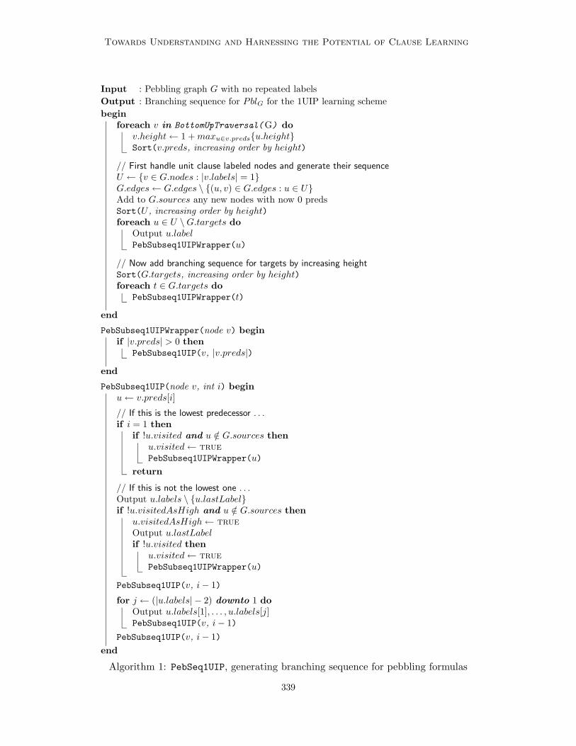
Towards Understanding and Harnessing the Potential of Clause Learning
Input : Pebbling graph G with no repeated labels
Output : Branching sequence for PblG for the 1UIP learning scheme
beginforeach v in BottomUpTraversal(G) do
v.height← 1 + maxu∈v.predsu.heightSort(v.preds, increasing order by height)
// First handle unit clause labeled nodes and generate their sequenceU ← v ∈ G.nodes : |v.labels| = 1G.edges← G.edges \ (u, v) ∈ G.edges : u ∈ UAdd to G.sources any new nodes with now 0 predsSort(U , increasing order by height)foreach u ∈ U \G.targets do
Output u.labelPebSubseq1UIPWrapper(u)
// Now add branching sequence for targets by increasing heightSort(G.targets, increasing order by height)foreach t ∈ G.targets do
PebSubseq1UIPWrapper(t)
end
PebSubseq1UIPWrapper(node v) beginif |v.preds| > 0 then
PebSubseq1UIP(v, |v.preds|)
end
PebSubseq1UIP(node v, int i) beginu← v.preds[i]
// If this is the lowest predecessor . . .if i = 1 then
if !u.visited and u /∈ G.sources thenu.visited← true
PebSubseq1UIPWrapper(u)
return
// If this is not the lowest one . . .Output u.labels \ u.lastLabelif !u.visitedAsHigh and u /∈ G.sources then
u.visitedAsHigh← true
Output u.lastLabelif !u.visited then
u.visited← true
PebSubseq1UIPWrapper(u)
PebSubseq1UIP(v, i− 1)
for j ← (|u.labels| − 2) downto 1 doOutput u.labels[1], . . . , u.labels[j]PebSubseq1UIP(v, i− 1)
PebSubseq1UIP(v, i− 1)
end
Algorithm 1: PebSeq1UIP, generating branching sequence for pebbling formulas
339
Beame, Kautz, & Sabharwal
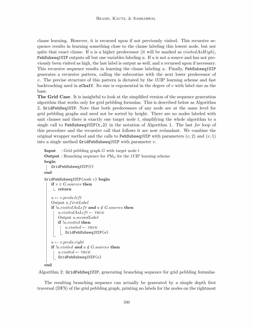
clause learning. However, it is recursed upon if not previously visited. This recursive se-quence results in learning something close to the clause labeling this lowest node, but notquite that exact clause. If u is a higher predecessor (it will be marked as visitedAsHigh),PebSubseq1UIP outputs all but one variables labeling u. If u is not a source and has not pre-viously been visited as high, the last label is output as well, and u recursed upon if necessary.This recursive sequence results in learning the clause labeling u. Finally, PebSubseq1UIPgenerates a recursive pattern, calling the subroutine with the next lower predecessor ofv. The precise structure of this pattern is dictated by the 1UIP learning scheme and fastbacktracking used in zChaff. Its size is exponential in the degree of v with label size as thebase.The Grid Case. It is insightful to look at the simplified version of the sequence generationalgorithm that works only for grid pebbling formulas. This is described below as Algorithm2, GridPebSeq1UIP. Note that both predecessors of any node are at the same level forgrid pebbling graphs and need not be sorted by height. There are no nodes labeled withunit clauses and there is exactly one target node t, simplifying the whole algorithm to asingle call to PebSubseq1UIP(t,2) in the notation of Algorithm 1. The last for loop ofthis procedure and the recursive call that follows it are now redundant. We combine theoriginal wrapper method and the calls to PebSubseq1UIP with parameters (v, 2) and (v, 1)into a single method GridPebSubseq1UIP with parameter v.
Input : Grid pebbling graph G with target node t
Output : Branching sequence for PblG for the 1UIP learning scheme
beginGridPebSubseq1UIP(t)
end
GridPebSubseq1UIP(node v) beginif v ∈ G.sources then
return
u← v.preds.leftOutput u.firstLabelif !u.visitedAsLeft and u /∈ G.sources then
u.visitedAsLeft← true
Output u.secondLabelif !u.visited then
u.visited← true
GridPebSubseq1UIP(u)
u← v.preds.rightif !u.visited and u /∈ G.sources then
u.visited← true
GridPebSubseq1UIP(u)
end
Algorithm 2: GridPebSeq1UIP, generating branching sequence for grid pebbling formulas
The resulting branching sequence can actually be generated by a simple depth firsttraversal (DFS) of the grid pebbling graph, printing no labels for the nodes on the rightmost
340
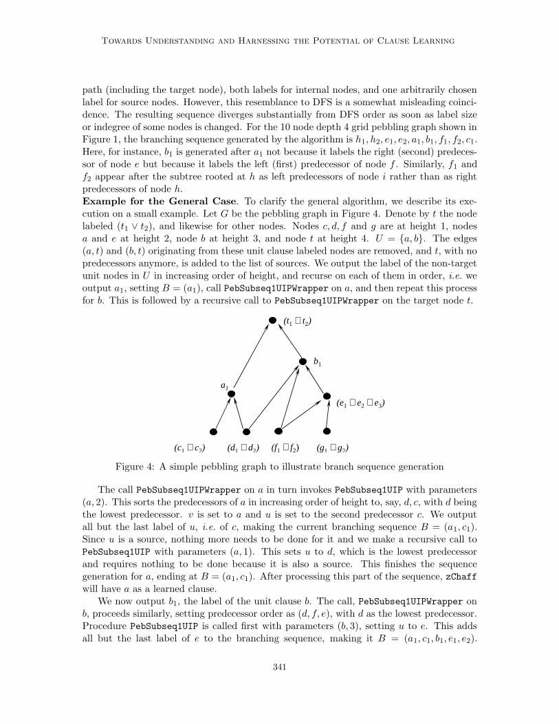
Towards Understanding and Harnessing the Potential of Clause Learning
path (including the target node), both labels for internal nodes, and one arbitrarily chosenlabel for source nodes. However, this resemblance to DFS is a somewhat misleading coinci-dence. The resulting sequence diverges substantially from DFS order as soon as label sizeor indegree of some nodes is changed. For the 10 node depth 4 grid pebbling graph shown inFigure 1, the branching sequence generated by the algorithm is h1, h2, e1, e2, a1, b1, f1, f2, c1.Here, for instance, b1 is generated after a1 not because it labels the right (second) predeces-sor of node e but because it labels the left (first) predecessor of node f . Similarly, f1 andf2 appear after the subtree rooted at h as left predecessors of node i rather than as rightpredecessors of node h.Example for the General Case. To clarify the general algorithm, we describe its exe-cution on a small example. Let G be the pebbling graph in Figure 4. Denote by t the nodelabeled (t1 ∨ t2), and likewise for other nodes. Nodes c, d, f and g are at height 1, nodesa and e at height 2, node b at height 3, and node t at height 4. U = a, b. The edges(a, t) and (b, t) originating from these unit clause labeled nodes are removed, and t, with nopredecessors anymore, is added to the list of sources. We output the label of the non-targetunit nodes in U in increasing order of height, and recurse on each of them in order, i.e. weoutput a1, setting B = (a1), call PebSubseq1UIPWrapper on a, and then repeat this processfor b. This is followed by a recursive call to PebSubseq1UIPWrapper on the target node t.
a1
b1
(t1 ∨ t2)
(c1 ∨ c2) (d1 ∨ d2) (f1 ∨ f2) (g1 ∨ g2)
(e1 ∨ e2 ∨ e3)
Figure 4: A simple pebbling graph to illustrate branch sequence generation
The call PebSubseq1UIPWrapper on a in turn invokes PebSubseq1UIP with parameters(a, 2). This sorts the predecessors of a in increasing order of height to, say, d, c, with d beingthe lowest predecessor. v is set to a and u is set to the second predecessor c. We outputall but the last label of u, i.e. of c, making the current branching sequence B = (a1, c1).Since u is a source, nothing more needs to be done for it and we make a recursive call toPebSubseq1UIP with parameters (a, 1). This sets u to d, which is the lowest predecessorand requires nothing to be done because it is also a source. This finishes the sequencegeneration for a, ending at B = (a1, c1). After processing this part of the sequence, zChaffwill have a as a learned clause.
We now output b1, the label of the unit clause b. The call, PebSubseq1UIPWrapper onb, proceeds similarly, setting predecessor order as (d, f, e), with d as the lowest predecessor.Procedure PebSubseq1UIP is called first with parameters (b, 3), setting u to e. This addsall but the last label of e to the branching sequence, making it B = (a1, c1, b1, e1, e2).
341
Beame, Kautz, & Sabharwal
Since this is the first time e is being visited as high, its last label is also added, makingB = (a1, c1, b1, e1, e2, e3), and it is recursed upon with PebSubseq1UIPWrapper(e). Thisrecursion extends the sequence to B = (a1, c1, b1, e1, e2, e3, f1). After processing this partof B, zChaff will have both a and (e1 ∨ e2 ∨ e3) as learned clauses. Getting to the secondhighest predecessor f of b, which happens to be a source, we simply add another f1 to B.Finally, we get to the third highest predecessor d of b, which happens to be the lowest aswell as a source, thus requiring nothing to be done. Coming out of the recursion, backto u = f , we generate the pattern given by the last for loop, which is empty becausethe label size of f is only 2. Coming out once more of the recursion to u = e, the for
loop pattern generates e1, f1 and is followed by a call to PebSubseq1UIP with the nextlower predecessor f as the second parameter, which generates f1. This makes the currentsequence B = (a1, c1, b1, e1, e2, e3, f1, f1, e1, f1, f1). After processing this, zChaff will alsohave b as a learned clause.
The final call to PebSubseq1UIPWrapper with parameter t doesn’t do anything becauseboth predecessors of t were removed in the beginning. Since both a and b have beenlearned, zChaff will have an immediate contradiction at decision level zero. This gives usthe complete branching sequence B = (a1, c1, b1, e1, e2, e3, f1, f1, e1, f1, f1) for the pebblingformula PblG.
6.1.2 Complexity of Sequence Generation
Let graph G have n nodes, indegree of non-source nodes between dmin and dmax, and labelsize between lmin and lmax. For simplicity of analysis, we will assume that lmin = lmax = land dmin = dmax = d (l = d = 2 for a grid graph).
Let us first compute the size of the pebbling formula associated with G. The runningtime of PebSeq1UIP and the size of the branching sequence generated will be given in termsof this size. The number of clauses in the pebbling formula PblG is roughly nld. Takingclause sizes into account, the size of the formula, |PblG|, is roughly n(l + d)ld. Note thatthe size of the CNF formula itself grows exponentially with the indegree and gets worseas label size increases. The best case is when G is the grid graph, where |PblG| = Θ(n).This explains the degradation in performance of zChaff, both original and modified, as wemove from grid graphs to random graphs (see section 6.3). Since we construct PblSAT
G bydeleting exactly one randomly chosen clause from PblG (see Section 2.5), the size |PblSAT
G |of the satisfiable version is also essentially the same.
Let us now compute the running time of PebSeq1UIP. Initial computation of heightsand predecessor sorting takes time Θ(nd log d). Assuming nu unit clause labeled nodesand nt target nodes, the remaining node sorting time is Θ(nu log nu + nt log nt). SincePebSubseq1UIPWrapper is called at most once for each node, the total running time ofPebSeq1UIP is Θ(nd log d + nu log nu + nt log nt + nTwrapper), where Twrapper denotes therunning time of PebSubseq1UIP- Wrapper without taking into account recursive calls toitself. When nu and nt are much smaller than n, which we will assume as the typicalcase, this simplifies to Θ(nd log d + nTwrapper). If T (v, i) denotes the running time ofPebSubseq1UIP(v,i), again without including recursive calls to the wrapper method, thenTwrapper = T (v, d). However, T (v, d) = lT (v, d−1)+Θ(l), which gives Twrapper = T (v, d) =
342
Towards Understanding and Harnessing the Potential of Clause Learning
Θ(ld+1). Substituting this back, we get that the running time of PebSeq1UIP is Θ(nld+1),which is about the same as |PblG|.
Finally, we consider the size of the branching sequence generated. Note that for eachnode, most of its contribution to the sequence is from the recursive pattern generated nearthe end of PebSubseq1UIP. Let Q(v, i) denote this contribution. Q(v, i) = (l − 2)(Q(v, i−1) + Θ(l)), which gives Q(v, i) = Θ(ld+2). Hence, the size of the sequence generated isΘ(nld+2), which again is about the same as |PblG|.
Theorem 3. Given a pebbling graph G with label size at most l and indegree of non-sourcenodes at most d, algorithm PebSeq1UIP produces a branching sequence σ of size at most Sin time Θ(dS), where S = |PblG| ≈ |PblSAT
G |. Moreover, the sequence σ is complete forPblG as well as for PblSAT
G under any clause learning algorithm using fast backtracking and1UIP learning scheme (such as zChaff).
Proof. The size and running time bounds follow from the previous discussion in this section.That this sequence is complete can be verified by a simple hand calculation simulating clauselearning with fast backtracking and 1UIP learning scheme.
6.2 Solving GTn Formulas
While pebbling formulas are not so easy to solve by popular SAT solvers, they are inherentlynot too difficult for clause learning algorithms. In fact, even without any learning, theyadmit tree-like proofs under a somewhat stronger related proof system, RES(k), for largeenough k:
Proposition 6 (Esteban et al., 2002). PblG has a size O(|G|) tree-like RES(k) refutation,where k is the maximum width of a clause labeling a node of G. In particular, when G is agrid graph with n nodes, PblG has an O(n) size tree-like RES(2) refutation.
Here RES(k) denotes the extension of RES that allows resolving, instead of clauses, dis-junctions of conjunctions of up to k literals (Krajıcek, 2001). RES(1) is simply RES. Proposi-tion 6 implies that addition of natural extension variables corresponding to k-conjunctionsof variables of PblG leads to O(|G| · k) size tree-like resolution proofs of related pebblingformulas PblG(k) (Atserias & Bonet, 2002).
For GTn formulas, however, no such short tree-like proofs are known in RES(k) for anyk. Reusing derived clauses (equivalently, learning clauses with DPLL) seems to be the key tofinding short proofs of GTn. This makes them a good candidate for testing clause learningbased SAT solvers. Our experiments indicate that GTn formulas, despite their simplicity,are quite hard for default zChaff. Using a good branching sequence based on the orderingstructure underlying these formulas leads to significant performance gains. Recall thatPebSeq1UIP was a fairly complex algorithm that generated a perfect branching sequencefor randomized pebbling graphs. In contrast, the branching sequence we give below forGTn formulas is generated by a nearly trivial algorithm. It is an incomplete sequence (seeDefinition 4) but boosts performance in practice.
6.2.1 Automatic Sequence Generation: GTnSeq1UIP
Since there is exactly one, well defined, unsatisfiable GT formula for a fixed parameter n,the approximate branching sequence given in Figure 5 below is straightforward. However,
343
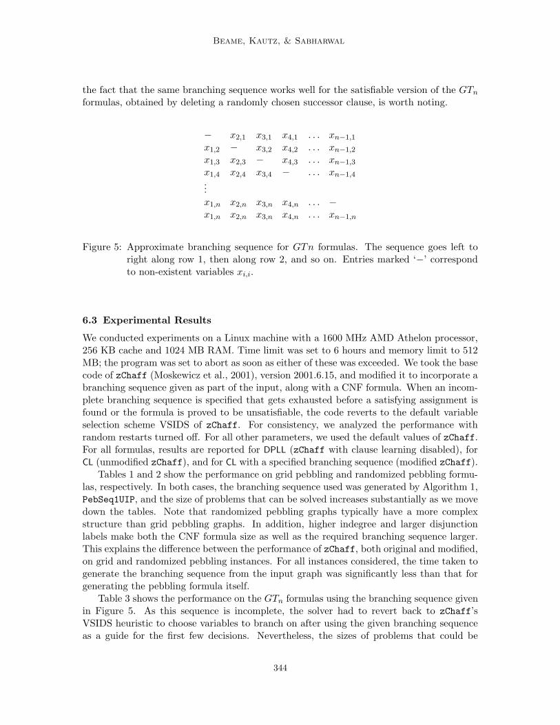
Beame, Kautz, & Sabharwal
the fact that the same branching sequence works well for the satisfiable version of the GTn
formulas, obtained by deleting a randomly chosen successor clause, is worth noting.
− x2,1 x3,1 x4,1 . . . xn−1,1
x1,2 − x3,2 x4,2 . . . xn−1,2
x1,3 x2,3 − x4,3 . . . xn−1,3
x1,4 x2,4 x3,4 − . . . xn−1,4...x1,n x2,n x3,n x4,n . . . −x1,n x2,n x3,n x4,n . . . xn−1,n
Figure 5: Approximate branching sequence for GTn formulas. The sequence goes left toright along row 1, then along row 2, and so on. Entries marked ‘−’ correspondto non-existent variables xi,i.
6.3 Experimental Results
We conducted experiments on a Linux machine with a 1600 MHz AMD Athelon processor,256 KB cache and 1024 MB RAM. Time limit was set to 6 hours and memory limit to 512MB; the program was set to abort as soon as either of these was exceeded. We took the basecode of zChaff (Moskewicz et al., 2001), version 2001.6.15, and modified it to incorporate abranching sequence given as part of the input, along with a CNF formula. When an incom-plete branching sequence is specified that gets exhausted before a satisfying assignment isfound or the formula is proved to be unsatisfiable, the code reverts to the default variableselection scheme VSIDS of zChaff. For consistency, we analyzed the performance withrandom restarts turned off. For all other parameters, we used the default values of zChaff.For all formulas, results are reported for DPLL (zChaff with clause learning disabled), forCL (unmodified zChaff), and for CL with a specified branching sequence (modified zChaff).
Tables 1 and 2 show the performance on grid pebbling and randomized pebbling formu-las, respectively. In both cases, the branching sequence used was generated by Algorithm 1,PebSeq1UIP, and the size of problems that can be solved increases substantially as we movedown the tables. Note that randomized pebbling graphs typically have a more complexstructure than grid pebbling graphs. In addition, higher indegree and larger disjunctionlabels make both the CNF formula size as well as the required branching sequence larger.This explains the difference between the performance of zChaff, both original and modified,on grid and randomized pebbling instances. For all instances considered, the time taken togenerate the branching sequence from the input graph was significantly less than that forgenerating the pebbling formula itself.
Table 3 shows the performance on the GTn formulas using the branching sequence givenin Figure 5. As this sequence is incomplete, the solver had to revert back to zChaff’sVSIDS heuristic to choose variables to branch on after using the given branching sequenceas a guide for the first few decisions. Nevertheless, the sizes of problems that could be
344
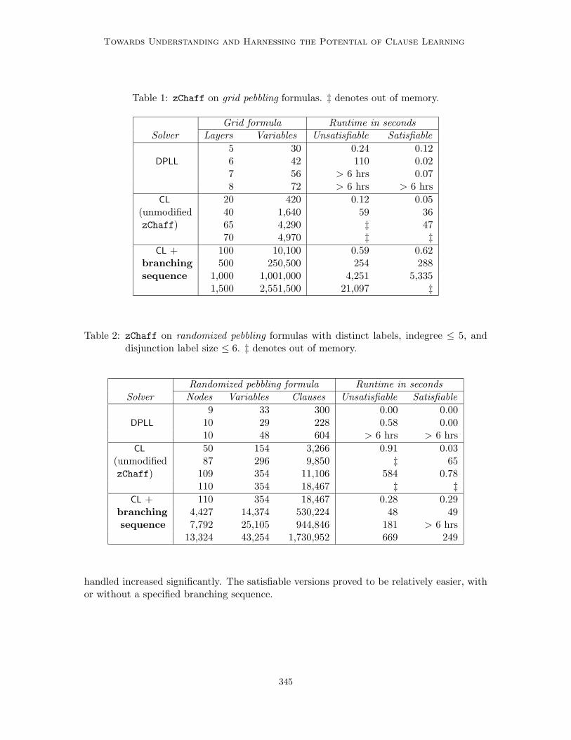
Towards Understanding and Harnessing the Potential of Clause Learning
Table 1: zChaff on grid pebbling formulas. ‡ denotes out of memory.
Grid formula Runtime in secondsSolver Layers Variables Unsatisfiable Satisfiable
5 30 0.24 0.12DPLL 6 42 110 0.02
7 56 > 6 hrs 0.078 72 > 6 hrs > 6 hrs
CL 20 420 0.12 0.05(unmodified 40 1,640 59 36zChaff) 65 4,290 ‡ 47
70 4,970 ‡ ‡
CL + 100 10,100 0.59 0.62branching 500 250,500 254 288sequence 1,000 1,001,000 4,251 5,335
1,500 2,551,500 21,097 ‡
Table 2: zChaff on randomized pebbling formulas with distinct labels, indegree ≤ 5, anddisjunction label size ≤ 6. ‡ denotes out of memory.
Randomized pebbling formula Runtime in secondsSolver Nodes Variables Clauses Unsatisfiable Satisfiable
9 33 300 0.00 0.00DPLL 10 29 228 0.58 0.00
10 48 604 > 6 hrs > 6 hrs
CL 50 154 3,266 0.91 0.03(unmodified 87 296 9,850 ‡ 65zChaff) 109 354 11,106 584 0.78
110 354 18,467 ‡ ‡
CL + 110 354 18,467 0.28 0.29branching 4,427 14,374 530,224 48 49sequence 7,792 25,105 944,846 181 > 6 hrs
13,324 43,254 1,730,952 669 249
handled increased significantly. The satisfiable versions proved to be relatively easier, withor without a specified branching sequence.
345
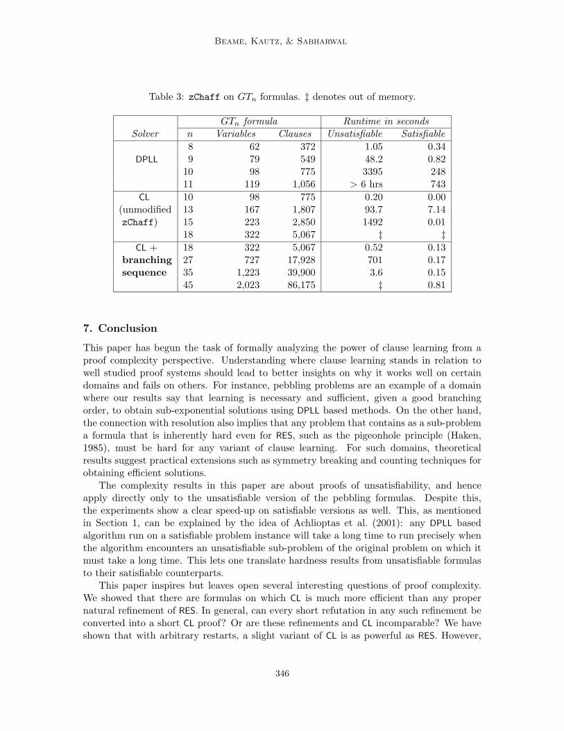
Beame, Kautz, & Sabharwal
Table 3: zChaff on GTn formulas. ‡ denotes out of memory.
GTn formula Runtime in secondsSolver n Variables Clauses Unsatisfiable Satisfiable
8 62 372 1.05 0.34DPLL 9 79 549 48.2 0.82
10 98 775 3395 24811 119 1,056 > 6 hrs 743
CL 10 98 775 0.20 0.00(unmodified 13 167 1,807 93.7 7.14zChaff) 15 223 2,850 1492 0.01
18 322 5,067 ‡ ‡
CL + 18 322 5,067 0.52 0.13branching 27 727 17,928 701 0.17sequence 35 1,223 39,900 3.6 0.15
45 2,023 86,175 ‡ 0.81
7. Conclusion
This paper has begun the task of formally analyzing the power of clause learning from aproof complexity perspective. Understanding where clause learning stands in relation towell studied proof systems should lead to better insights on why it works well on certaindomains and fails on others. For instance, pebbling problems are an example of a domainwhere our results say that learning is necessary and sufficient, given a good branchingorder, to obtain sub-exponential solutions using DPLL based methods. On the other hand,the connection with resolution also implies that any problem that contains as a sub-problema formula that is inherently hard even for RES, such as the pigeonhole principle (Haken,1985), must be hard for any variant of clause learning. For such domains, theoreticalresults suggest practical extensions such as symmetry breaking and counting techniques forobtaining efficient solutions.
The complexity results in this paper are about proofs of unsatisfiability, and henceapply directly only to the unsatisfiable version of the pebbling formulas. Despite this,the experiments show a clear speed-up on satisfiable versions as well. This, as mentionedin Section 1, can be explained by the idea of Achlioptas et al. (2001): any DPLL basedalgorithm run on a satisfiable problem instance will take a long time to run precisely whenthe algorithm encounters an unsatisfiable sub-problem of the original problem on which itmust take a long time. This lets one translate hardness results from unsatisfiable formulasto their satisfiable counterparts.
This paper inspires but leaves open several interesting questions of proof complexity.We showed that there are formulas on which CL is much more efficient than any propernatural refinement of RES. In general, can every short refutation in any such refinement beconverted into a short CL proof? Or are these refinements and CL incomparable? We haveshown that with arbitrary restarts, a slight variant of CL is as powerful as RES. However,
346
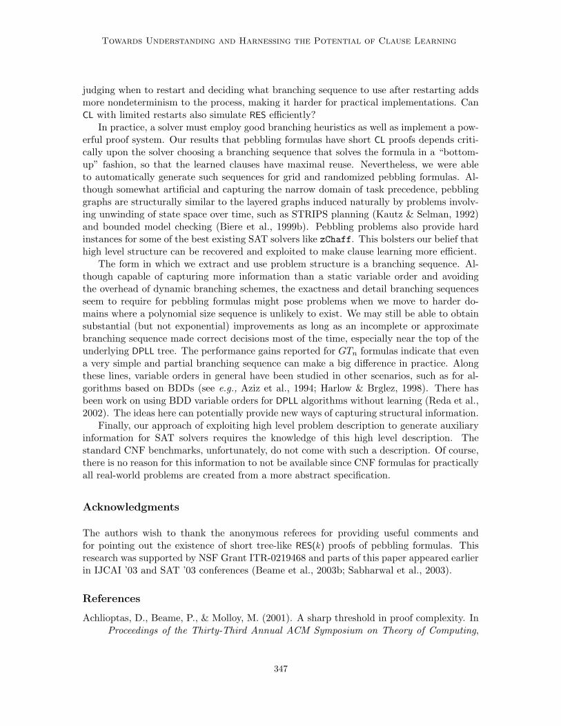
Towards Understanding and Harnessing the Potential of Clause Learning
judging when to restart and deciding what branching sequence to use after restarting addsmore nondeterminism to the process, making it harder for practical implementations. CanCL with limited restarts also simulate RES efficiently?
In practice, a solver must employ good branching heuristics as well as implement a pow-erful proof system. Our results that pebbling formulas have short CL proofs depends criti-cally upon the solver choosing a branching sequence that solves the formula in a “bottom-up” fashion, so that the learned clauses have maximal reuse. Nevertheless, we were ableto automatically generate such sequences for grid and randomized pebbling formulas. Al-though somewhat artificial and capturing the narrow domain of task precedence, pebblinggraphs are structurally similar to the layered graphs induced naturally by problems involv-ing unwinding of state space over time, such as STRIPS planning (Kautz & Selman, 1992)and bounded model checking (Biere et al., 1999b). Pebbling problems also provide hardinstances for some of the best existing SAT solvers like zChaff. This bolsters our belief thathigh level structure can be recovered and exploited to make clause learning more efficient.
The form in which we extract and use problem structure is a branching sequence. Al-though capable of capturing more information than a static variable order and avoidingthe overhead of dynamic branching schemes, the exactness and detail branching sequencesseem to require for pebbling formulas might pose problems when we move to harder do-mains where a polynomial size sequence is unlikely to exist. We may still be able to obtainsubstantial (but not exponential) improvements as long as an incomplete or approximatebranching sequence made correct decisions most of the time, especially near the top of theunderlying DPLL tree. The performance gains reported for GTn formulas indicate that evena very simple and partial branching sequence can make a big difference in practice. Alongthese lines, variable orders in general have been studied in other scenarios, such as for al-gorithms based on BDDs (see e.g., Aziz et al., 1994; Harlow & Brglez, 1998). There hasbeen work on using BDD variable orders for DPLL algorithms without learning (Reda et al.,2002). The ideas here can potentially provide new ways of capturing structural information.
Finally, our approach of exploiting high level problem description to generate auxiliaryinformation for SAT solvers requires the knowledge of this high level description. Thestandard CNF benchmarks, unfortunately, do not come with such a description. Of course,there is no reason for this information to not be available since CNF formulas for practicallyall real-world problems are created from a more abstract specification.
Acknowledgments
The authors wish to thank the anonymous referees for providing useful comments andfor pointing out the existence of short tree-like RES(k) proofs of pebbling formulas. Thisresearch was supported by NSF Grant ITR-0219468 and parts of this paper appeared earlierin IJCAI ’03 and SAT ’03 conferences (Beame et al., 2003b; Sabharwal et al., 2003).
References
Achlioptas, D., Beame, P., & Molloy, M. (2001). A sharp threshold in proof complexity. InProceedings of the Thirty-Third Annual ACM Symposium on Theory of Computing,
347
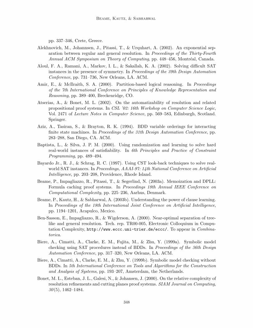
Beame, Kautz, & Sabharwal
pp. 337–346, Crete, Greece.
Alekhnovich, M., Johannsen, J., Pitassi, T., & Urquhart, A. (2002). An exponential sep-aration between regular and general resolution. In Proceedings of the Thirty-FourthAnnual ACM Symposium on Theory of Computing, pp. 448–456, Montreal, Canada.
Aloul, F. A., Ramani, A., Markov, I. L., & Sakallah, K. A. (2002). Solving difficult SATinstances in the presence of symmetry. In Proceedings of the 39th Design AutomationConference, pp. 731–736, New Orleans, LA. ACM.
Amir, E., & McIlraith, S. A. (2000). Partition-based logical reasoning. In Proceedingsof the 7th International Conference on Principles of Knowledge Representation andReasoning, pp. 389–400, Breckenridge, CO.
Atserias, A., & Bonet, M. L. (2002). On the automatizability of resolution and relatedpropositional proof systems. In CSL ’02: 16th Workshop on Computer Science Logic,Vol. 2471 of Lecture Notes in Computer Science, pp. 569–583, Edinburgh, Scotland.Springer.
Aziz, A., Tasiran, S., & Brayton, R. K. (1994). BDD variable orderings for interactingfinite state machines. In Proceedings of the 31th Design Automation Conference, pp.283–288, San Diego, CA. ACM.
Baptista, L., & Silva, J. P. M. (2000). Using randomization and learning to solve hardreal-world instances of satisfiability. In 6th Principles and Practice of ConstraintProgramming, pp. 489–494.
Bayardo Jr., R. J., & Schrag, R. C. (1997). Using CST look-back techniques to solve real-world SAT instances. In Proceedings, AAAI-97: 14th National Conference on ArtificialIntelligence, pp. 203–208, Providence, Rhode Island.
Beame, P., Impagliazzo, R., Pitassi, T., & Segerlind, N. (2003a). Memoization and DPLL:Formula caching proof systems. In Proceedings 18th Annual IEEE Conference onComputational Complexity, pp. 225–236, Aarhus, Denmark.
Beame, P., Kautz, H., & Sabharwal, A. (2003b). Understanding the power of clause learning.In Proceedings of the 18th International Joint Conference on Artificial Intelligence,pp. 1194–1201, Acapulco, Mexico.
Ben-Sasson, E., Impagliazzo, R., & Wigderson, A. (2000). Near-optimal separation of tree-like and general resolution. Tech. rep. TR00-005, Electronic Colloquium in Compu-tation Complexity, http://www.eccc.uni-trier.de/eccc/. To appear in Combina-torica.
Biere, A., Cimatti, A., Clarke, E. M., Fujita, M., & Zhu, Y. (1999a). Symbolic modelchecking using SAT procedures instead of BDDs. In Proceedings of the 36th DesignAutomation Conference, pp. 317–320, New Orleans, LA. ACM.
Biere, A., Cimatti, A., Clarke, E. M., & Zhu, Y. (1999b). Symbolic model checking withoutBDDs. In 5th International Conference on Tools and Algorithms for the Constructionand Analysis of Systems, pp. 193–207, Amsterdam, the Netherlands.
Bonet, M. L., Esteban, J. L., Galesi, N., & Johansen, J. (2000). On the relative complexity ofresolution refinements and cutting planes proof systems. SIAM Journal on Computing,30 (5), 1462–1484.
348
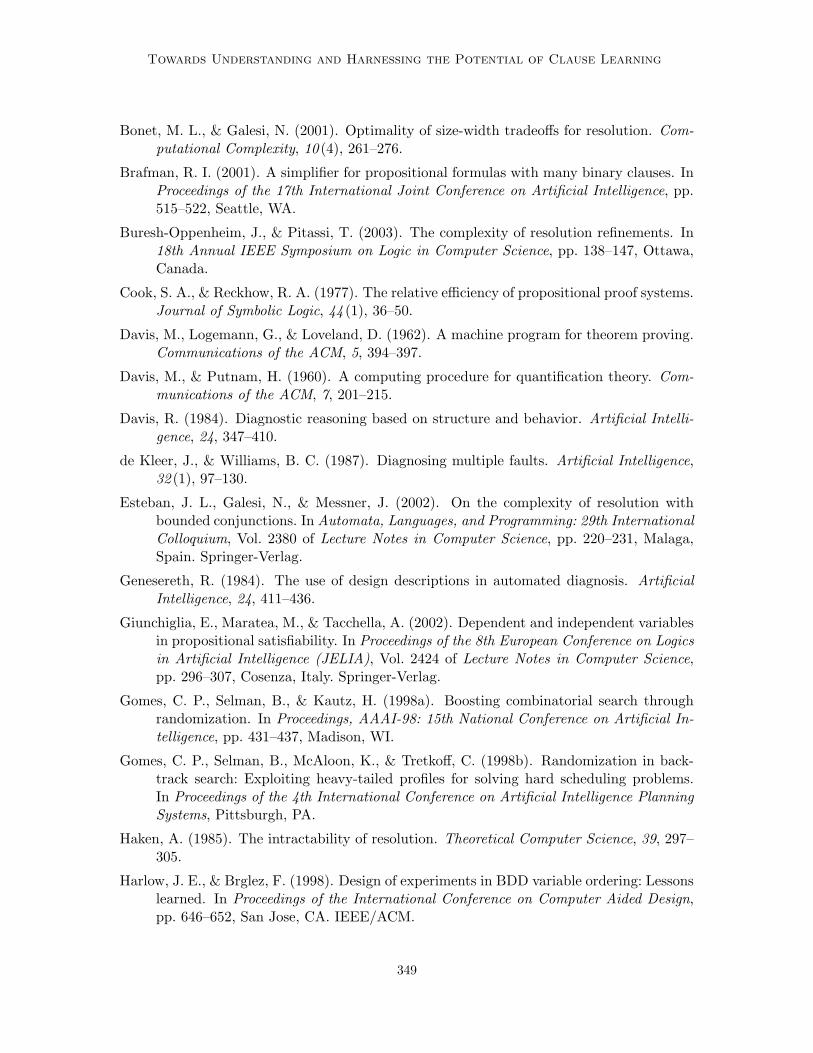
Towards Understanding and Harnessing the Potential of Clause Learning
Bonet, M. L., & Galesi, N. (2001). Optimality of size-width tradeoffs for resolution. Com-putational Complexity, 10 (4), 261–276.
Brafman, R. I. (2001). A simplifier for propositional formulas with many binary clauses. InProceedings of the 17th International Joint Conference on Artificial Intelligence, pp.515–522, Seattle, WA.
Buresh-Oppenheim, J., & Pitassi, T. (2003). The complexity of resolution refinements. In18th Annual IEEE Symposium on Logic in Computer Science, pp. 138–147, Ottawa,Canada.
Cook, S. A., & Reckhow, R. A. (1977). The relative efficiency of propositional proof systems.Journal of Symbolic Logic, 44 (1), 36–50.
Davis, M., Logemann, G., & Loveland, D. (1962). A machine program for theorem proving.Communications of the ACM, 5, 394–397.
Davis, M., & Putnam, H. (1960). A computing procedure for quantification theory. Com-munications of the ACM, 7, 201–215.
Davis, R. (1984). Diagnostic reasoning based on structure and behavior. Artificial Intelli-gence, 24, 347–410.
de Kleer, J., & Williams, B. C. (1987). Diagnosing multiple faults. Artificial Intelligence,32 (1), 97–130.
Esteban, J. L., Galesi, N., & Messner, J. (2002). On the complexity of resolution withbounded conjunctions. In Automata, Languages, and Programming: 29th InternationalColloquium, Vol. 2380 of Lecture Notes in Computer Science, pp. 220–231, Malaga,Spain. Springer-Verlag.
Genesereth, R. (1984). The use of design descriptions in automated diagnosis. ArtificialIntelligence, 24, 411–436.
Giunchiglia, E., Maratea, M., & Tacchella, A. (2002). Dependent and independent variablesin propositional satisfiability. In Proceedings of the 8th European Conference on Logicsin Artificial Intelligence (JELIA), Vol. 2424 of Lecture Notes in Computer Science,pp. 296–307, Cosenza, Italy. Springer-Verlag.
Gomes, C. P., Selman, B., & Kautz, H. (1998a). Boosting combinatorial search throughrandomization. In Proceedings, AAAI-98: 15th National Conference on Artificial In-telligence, pp. 431–437, Madison, WI.
Gomes, C. P., Selman, B., McAloon, K., & Tretkoff, C. (1998b). Randomization in back-track search: Exploiting heavy-tailed profiles for solving hard scheduling problems.In Proceedings of the 4th International Conference on Artificial Intelligence PlanningSystems, Pittsburgh, PA.
Haken, A. (1985). The intractability of resolution. Theoretical Computer Science, 39, 297–305.
Harlow, J. E., & Brglez, F. (1998). Design of experiments in BDD variable ordering: Lessonslearned. In Proceedings of the International Conference on Computer Aided Design,pp. 646–652, San Jose, CA. IEEE/ACM.
349
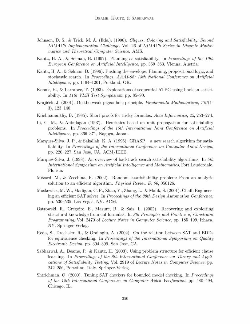
Beame, Kautz, & Sabharwal
Johnson, D. S., & Trick, M. A. (Eds.). (1996). Cliques, Coloring and Satisfiability: SecondDIMACS Implementation Challenge, Vol. 26 of DIMACS Series in Discrete Mathe-matics and Theoretical Computer Science. AMS.
Kautz, H. A., & Selman, B. (1992). Planning as satisfiability. In Proceedings of the 10thEuropean Conference on Artificial Intelligence, pp. 359–363, Vienna, Austria.
Kautz, H. A., & Selman, B. (1996). Pushing the envelope: Planning, propositional logic, andstochastic search. In Proceedings, AAAI-96: 13th National Conference on ArtificialIntelligence, pp. 1194–1201, Portland, OR.
Konuk, H., & Larrabee, T. (1993). Explorations of sequential ATPG using boolean satisfi-ability. In 11th VLSI Test Symposium, pp. 85–90.
Krajıcek, J. (2001). On the weak pigeonhole principle. Fundamenta Mathematicae, 170 (1-3), 123–140.
Krishnamurthy, B. (1985). Short proofs for tricky formulas. Acta Informatica, 22, 253–274.
Li, C. M., & Anbulagan (1997). Heuristics based on unit propagation for satisfiabilityproblems. In Proceedings of the 15th International Joint Conference on ArtificialIntelligence, pp. 366–371, Nagoya, Japan.
Marques-Silva, J. P., & Sakallah, K. A. (1996). GRASP – a new search algorithm for satis-fiability. In Proceedings of the International Conference on Computer Aided Design,pp. 220–227, San Jose, CA. ACM/IEEE.
Marques-Silva, J. (1998). An overview of backtrack search satisfiability algorithms. In 5thInternational Symposium on Artificial Intelligence and Mathematics, Fort Lauderdale,Florida.
Mezard, M., & Zecchina, R. (2002). Random k-satisfiability problem: From an analyticsolution to an efficient algorithm. Physical Review E, 66, 056126.
Moskewicz, M. W., Madigan, C. F., Zhao, Y., Zhang, L., & Malik, S. (2001). Chaff: Engineer-ing an efficient SAT solver. In Proceedings of the 38th Design Automation Conference,pp. 530–535, Las Vegas, NV. ACM.
Ostrowski, R., Gregoire, E., Mazure, B., & Sais, L. (2002). Recovering and exploitingstructural knowledge from cnf formulas. In 8th Principles and Practice of ConstraintProgramming, Vol. 2470 of Lecture Notes in Computer Science, pp. 185–199, Ithaca,NY. Springer-Verlag.
Reda, S., Drechsler, R., & Orailoglu, A. (2002). On the relation between SAT and BDDsfor equivalence checking. In Proceedings of the International Symposium on QualityElectronic Design, pp. 394–399, San Jose, CA.
Sabharwal, A., Beame, P., & Kautz, H. (2003). Using problem structure for efficient clauselearning. In Proceedings of the 6th International Conference on Theory and Appli-cations of Satisfiability Testing, Vol. 2919 of Lecture Notes in Computer Science, pp.242–256, Portofino, Italy. Springer-Verlag.
Shtrichman, O. (2000). Tuning SAT checkers for bounded model checking. In Proceedingsof the 12th International Conference on Computer Aided Verification, pp. 480–494,Chicago, IL.
350
Towards Understanding and Harnessing the Potential of Clause Learning
Stallman, R., & Sussman, G. J. (1977). Forward reasoning and dependency-directed back-tracking in a system for computer-aided circuit analysis. Artificial Intelligence, 9,135–196.
Velev, M., & Bryant, R. (2001). Effective use of boolean satisfiability procedures in theformal verification of superscalar and vliw microprocessors. In Proceedings of the 38thDesign Automation Conference, pp. 226–231.
Zhang, H., & Hsiang, J. (1994). Solving open quasigroup problems by propositional reason-ing. In Proceedings of the International Computer Symp., Hsinchu, Taiwan.
Zhang, H. (1997). SATO: An efficient propositional prover. In Proceedings of the 14th Inter-national Conference on Automated Deduction, Vol. 1249 of Lecture Notes in ComputerScience, pp. 272–275, Townsville, Australia.
Zhang, L., Madigan, C. F., Moskewicz, M. H., & Malik, S. (2001). Efficient conflict drivenlearning in a boolean satisfiability solver. In Proceedings of the International Confer-ence on Computer Aided Design, pp. 279–285, San Jose, CA. IEEE/ACM.
351