Towards a Spatial Analysis Framework: Modelling Urban Development Patterns

CHENG JIANQUAN ; IAN MASSER (Jianquan@itc.nl) (masser@itc.nl)

Division of Urban Planning and Management

International Institute for Aerospace Survey and Earth Sciences, The Netherlands (ITC) P.O.Box 6, 7500 AA , Enschede, The Netherlands

Abstract. Urban expansion has been a hot topic not only in the management of sustainable development but also in the fields of remote sensing and GIS. Urban development is a complicated dynamic process involving in various actors with different patterns of behavior. Modeling an urban development pattern is the prerequisite to understand the process. This paper presents a preliminary spatial framework for such modeling and uses it for the analysis of a rapidly developing city. This framework starts with a multi-scale conceptual model, which aims to theoretically link planning hierarchy, multi-extent analysis and multi-resolution data. The multi-extent data analysis is the focus of this paper, which is divided into three scales: change probability (macro), change density (meso) and change intensity (micro). Multi-extent data analysis aims to seek distinguishing spatial determinants on three scales, which is able to bridge planning system and data scale. The data analysis is based on the integration of change patterns detection method and spatial logistic regression method. The former is utilized for univariate analysis and then hypothesis formation. The latter is employed for systematic modelling of multi-variables. The combination of both is proven to have strong capacity of interpretation. This framework is tested by a case study of Wuhan City, P.R.China. The multi-scale property discovered is helpful for understanding complicated process of urban development.

[Key Words]: Spatial framework, scale, multi-extent, change pattern detection, logistic regression.

1. INTRODUCTION

During the last 5 decades, a series of political events occurred in China (such as the establishment of new government in 1949, economic reform in 1978 and land reform in 1987) which has brought about unparalleled changes on the urban development of Chinese cities. These changes are indicated by the rapid urban growth in the period of industrialization before 1978 and large scale urban new- and redevelopment under the market economy especially after 1987 (Wu 1998; Gaubatz 1999). The exploration of the urban development process spanning so long a period is crucial to decision making and planning the form of future urban development.

With the rapid development of remote sensing and geographical information sciences (GIS) and techniques, they have been increasingly used to facilitate large-scale studies in urban development. Modern satellite imagary, together with traditional aerial photos provides rich multi- resolution and scale of data sources for monitoring urban development process. By using GIS , it is technically possible to integrate large quantities of data for further spatial analysis related to urban development.

However, it has become common knowledge that urban development is a complicated dynamic process, which involves various physical, social and economic factors.

The complexity lies in the unknown amount of factors, multi-scale interactions among factors and its unpredictable dynamics, which are beyond the capacities of current GIS theory and method. Pattern and process are reciprocally related like ‘egg and chicken’, and both of them and their relation are also scale dependent. The seek of determinant factors on varied scale is the first step to understand the dynamic process. Towards this purpose, we need to integrate RS, GIS and other modelling techniques for understanding the interaction between urban development patterns and processes.

Urban development is divided into urban growth and redevelopment, which are typically projected onto various scales of land cover and land-use change respectively (Stanilov 1998). Spatially explicit modelling of land-use changes is an important technique for describing processes of change in quantitative terms and for testing our understanding of these processes (Serneels and Lambin 2001). Consequently, modelling of land cover and land use change, as increasingly applied in the areas of agricultural, environmental and ecological systems (Schneider and Gil Pontius Jr. 2001; Walsh and Crawford 2001), is of crucial importance to understand the urban development process.

With these considerations in mind, this paper proposes a spatial analysis framework for modelling urban development patterns, which is centered by seeking varied determinants affecting land cover/land use change on various scales. Following the introduction,

section 2 discusses in detail the framework and the methods applied by other studies. Section 3 describes the case study area, followed by its database development based on remotely sensed sources and GIS. The 4th section focus on the modelling techniques to be applied, which comprise exploratory and confirmatory approach. Its multi-scale property is tested and analyzed in the study area. This paper ends up with further discussion of relevant issues and possible directions for future research.

2. A MULTI-SCALE SPATIAL ANALYSIS FRAMEWORK

Scale issues are inherent in studies examining the physical and human forces driving land use and land cover changes (Currit 2000). The term "scale" has multiple referents, including absolute size, relative size, resolution, granularity, extent and detail, which is one of the main concern of geo-computation. Regarding urban development, here multi-scale has three hierarchies of meaning (figure 1), which are interwoven one another. The first is on conceptual level, which is planning oriented system such as general land use

planning, urban master or structure planning and detailed control or zoning planning. Second is spatial extent or details of analysis to support the decision making of different level planning and management. The third is spatial and temporal resolution of data (data-scale), which will highly affect the reliability of spatial analysis. Spatial resolution is related to the size of grid defined in the case of raster data format. Temporal resolution is linked to the length of change period analyzed. The scale of spatial analysis is to bridge conceptual and data scale. Conceptual level determines the objective of spatial analysis. Data level not only provides required resolution (spatial and temporal) of data as input into modelling but also

seriously affect the results of modelling. Data collected at a gross scale (coarser resolution) is considered less reliable in aiding interpretation of events operating at fine scales (finer resolution) (Goodchild, 2000). This issue has been receiving more and more attentions especially in relevant application areas (Schneider and Gil Pontius Jr. 2001; Walsh and Crawford 2001). This paper will focus on the scale of spatial analysis, which is not paid adequate attentions in land cover/land use modelling although extent and resolution are not completely independent for practical reasons (Kok and Veldkamp 2001). Kok and Veldkamp in his research found that the effect of changing the spatial extent on the set of land use determining factors is substantial, with an strong increase in explanatory power when reducing the extent from regional to national.

In the case of Chinese cities, general land use planning need to know the major spatial determinants of change probability pattern from rural to urban area, which is able to guide sustainable land management. The master or structural planning need to know the principal spatial determinants influencing change density and change type such as different scale construction, which is helpful for the decision-making of site selection of major projects planned. The lowest level of detailed

control planning or zoning need to know the spatial factors affecting the change intensity, which is indicated by different floors of high-rise buildings. They will be utilized for the control of plot ratio etc.

Consequently, the scale of spatial analysis could be divided into three levels (figure 1): change probability (macro), change density (meso-) and change intensity (micro). The former two (change probability and density) is to understand urban new development pattern from the perspective of probability and density, which principally is centered by land cover change. The latter is to understand urban redevelopment pattern from the angle of intensity, i.e. the vertical development like

Hierarchy of Urban Development Planning System

Change Probability Pattern

(Macro-)

Change Density Pattern

(Meso-)

Change Intensity Pattern

(Micro-)

Multi-Extent of Data Analysis

Multi-Resolution of data analysis

Figure 1: A multi-scale spatial analysis framework for modelling

Conceptual Level

Analysis Level

Data Level

high-rise buildings. This paper will demonstrate the effects of spatial analysis scale on pattern modelling by only taking the change probability and density as an example. The same set of data will be applied for both, but their spatial extent are varied, change probability take change (from rural to urban) and no-change into

account; change density only consider change aspect.

In pattern modelling, the representative methods could be landscape pattern modeling (Chuvieco 1999), fractal and diffusion limit aggregation (DLA) modeling in urban growth pattern(Makse, Andrade et al. 1998), neural network in transportation/land use interaction pattern(Rodrigue 1997), neural network in land transformation modelling (Currit 2000), space syntax in urban development pattern (Desyllas, M. et al. 1997), logistic regression modeling in urban land use change (Morisette, Khorram et al. 1999). They are successful in either providing quantitative spatial indicators or offering systematic modelling tools. The former include fractal dimension (Shen 1997), global integration indicator to quantify geometric accessibility (Jiang, Claramunt et al. 1999), diversity index etc (Chuvieco 1999). These indicators are complex to be computed and lack of practical implication and comparability. The latter like neural network is a useful tool to systematically model non-linear system like city but the modeling procedure is not transparent due to a black box. By contrast, as a traditional statistical analysis technique, logistic regression, is receiving more and more attentions in pattern modelling due to its relatively stronger interpretation capacity (Pereira and Itami 1991; Gumpertz, Wu et al. 2000; Koutsias and Karteris 2000; Tang and Choy 2000; Serneels and Lambin 2001). For example, (Wu and Yeh 1997) (Wu 2000) applied logistic regression method for modelling land development pattern and industrial firm location respectively based on vector data format. The modeling has been proven to be effective in seeking some determining variables for the occurrence of certain spatial phenomena like urban development. However, first of all, the primary data sources regarding urban development especially urban growth come from

satellite images. Spatial/temporal resolution is becoming a main concern. In this case, logistic regression has to incorporate spatial issues like spatial dependence and spatial sampling when making model. The ignorance of these assumptions will lead to unreliable parameter estimation or inefficient estimates and false conclusions

regarding hypothesis tests (Irwin and Geoghegan 2001). Consequently, spatial statistics means has to be introduced into logistic regression, but they are sensitive to some assumptions. It is to argue that exploratory spatial data analysis should be integrated with logistic regression for pre- and post- modelling.

3. DATABASE DEVELOPMENT

3.1 Study Area

As the capital of Hubei Province, Wuhan is the largest mega city (> 1 million) in central China and in the middle reaches of Yangtze River (Map1). In 1999, it has more than 4 million urban populations, 4 times more than that of 1949. During the last 5 decades, Wuhan undergone rapid urban growth from 3000 ha in 1949 to 3,0151 ha in 2000 in built-up area, which went through two waves of development: 1955-1965 and 1993-2000. The two waves corresponded to the two major stimulants: rapid industrialization and land reform before and after 1987 (Cheng, Turkstra et al. 2001), which is consistent with the other Chinese cities like Guangzhou (Wu 1998). As a result, Wuhan is a fresh and typical case to understand the dynamic process of urban development of Chinese cities.

3.2 Data sources

Temporal mapping is the prerequisite of urban development pattern modelling. The widely recognized data sources primarily come from remotely sensed imaginary including satellite images and aerial photos. SPOT PAN/XS data is an ideal source to produce land cover maps at the urban-rural fringe (Quarmby and Cushnie 1989; Jensen 1996; Gao and Skillcorn 1998;

[2] Location of Wuhan in Hubei Province

[1] Location of Hubei in China

Wuha

Yangtze River

Hubei

Yangtz River

Wuhan

Han River

Map 1: Location of Wuhan city

Terrettaz 1998). The imaginary employed here includes SPOT PAN/XS in 1993, 2000, which cover the whole study area. The topographic map (1:10,000) of 1993 was used for imaginary geo-coding registration. The secondary sources include planning scheme maps, traffic/tourism maps, street boundary map etc. The image processing was implemented through ERDAS IMAGINE 8.4 package.

First, the original images are subset into appropriate size just covering the study area; a projection system of WGS84 NORTH with Zone 50 is selected for Wuhan City. At least 50 points are systematically chosen and evenly distributed over images to guarantee enough points in center and corners. Second order polynomial model is chosen for image rectification, re-sampled by using nearest-neighbor algorithm. The RMS error is strictly limited to 0.3 pixel.

Second, to assist visual interpretation, Image fusion is implemented to comprehensively harness the spectral information from SPOT XS (3 bands) and spatial information from SPOT PAN (10 m). Before fusion, the accurate co-registration is vital for the accuracy of fusion. A map-to-image strategy is applied for higher resolution of SPOT PAN based on the topographic map 1:10,000, and then the image-to-image method is used for the geo-referenced registration of SPOT XS. Adequate ground control points could guarantee the accurate position match of two images. Among the 3 resolution merge techniques (Multiplicative, principal component, brovey transform) in ERDAS, Multiplicative is chosen for the fusion as being better for highlighting urban features.

Third, before digitizing, the fused images are transferred into RGB images as the color composite. And then an un-supervised classification is made for seeking any pixels with potential land cover change. The final visual interpretation is carried out to remove mis-supervision with the assistance of local knowledge.

3.3 Data classification

The main information requirement for the modelling Wuhan growth pattern comprise land cover, physical factors (road network, railway lines, city center/sub-center, bridges, rivers) and socio-economic factors (population and employment), which are processed from primary and secondary sources. Socio-economic data is limited to population census of 1990 on sub-district level and yearly statistical data on district level. Land cover is here classified as water, town/village, green, agricultural, and urban built-up area. There is not a universal standard of road classification as it is determined by quite a number of factors like neighbouring land use, traffic volume, road width, and construction structure. It is the same for the definition of city center/sub-center. In this research, in order to reduce the uncertainty in road classification, only two classes (main roads and the rest) are adopted to identify

their impacts on urban development. The determination of main roads and city center are principally based on the local knowledge available from master and transportation planning schemes, and tourism maps, which actually affected the decision making of urban development. Some interviews with local planners are also made to gain necessary confirms.

The urban growth in the period 1993-2000 is displayed in map 2. The main factors like infrastructure and macro-level control can be seen from map 3 and 4 respectively.

3.4 The definition of Variables

The variables as described in table 1 are created via spatial analyst module in Arcview based on the 20 m cell size.

Dependent variables: for dependent variable CHANGE on macro level, The value “1” represents all new change (from rural to urban) (see Map 2 and 5), value “0” is the rural area without change (see ‘Developable Area’ in Map 2). The spatial extent of CHANGE is limited in the administrative boundary of Wuhan municipality then (Map 5). For dependent variable CH_DENSITY (Map 6) on meso level (change density), The value “1” represents high density of change; value “0” indicates the low density of change. Map2 shows that the urban growth in 1993-2000 was characterized by large scale spatial agglomeration. The agglomeration is principally represented by 4 new development zones (see Map 2. 1: Guandong and Guannan industrial parks; 2: Nanhu and Changhong industrial parks; 3:Zuankou Car Manufacturing Base; 4:Taiwanese Economic Development Zones). The calculation of change density is completed through ‘moving window’ method. A neighbourhood with 20*20 (16 ha) rectangle was defined to summarize the quantity of land cover change surrounding each pixel studied. With this neighbourhood, we are able to form a normal distribution for CH_DENSITY.

Independent variables: First, in the developed nations, proximity is a prime cause of urban expansion; transport and communication changes represent another major explanatory variable in helping to account for the continuing demand for urban land (Kivell 1993). Here, the proximity variables measure the direct access to city center/sub-center (DIST_CENT), main roads (DIST_MRD), other roads (DIST_ORD), railway lines (DIST_RAIL), Yangtze/Han rivers (DIST_RIVER), constructed bridges over Yangtze rive (DIST_CBRID) and planned bridges on Yangtze river (DIST_PBRID) respectively. The constructed bridges are No:1 (1957) and No:2 (1994) bridges over Yangtze river. The planned ones are Baishazhou (Lower reach) and Tianxinzhou (Upper reach). The spatial distribution of roads, railway bridges and centers/sub-centers is shown in Map 3.

Map 2: Urban Growth 1993-2000 and Developable, Developed and Water body

Map 3: Spatial Distribution of Roads, Railway Lines, Bridges and Centers in 1993-2000

[1] Industrial Sites in 1993 (DENS_INDU )

[2] Sub_districts and others in 1993 (STREET_NO)

[3] Master Planning 1996-2020 (PLAN_NO) [4] Three levels of population density (CPOP_DENS)

Map 4: Spatial distribution of Variables (DENS_INDU, STREET_NO, PLAN_NO, and CPOPU_DENS)

Map 5: Variable CHANGE and its Spatial Sampling

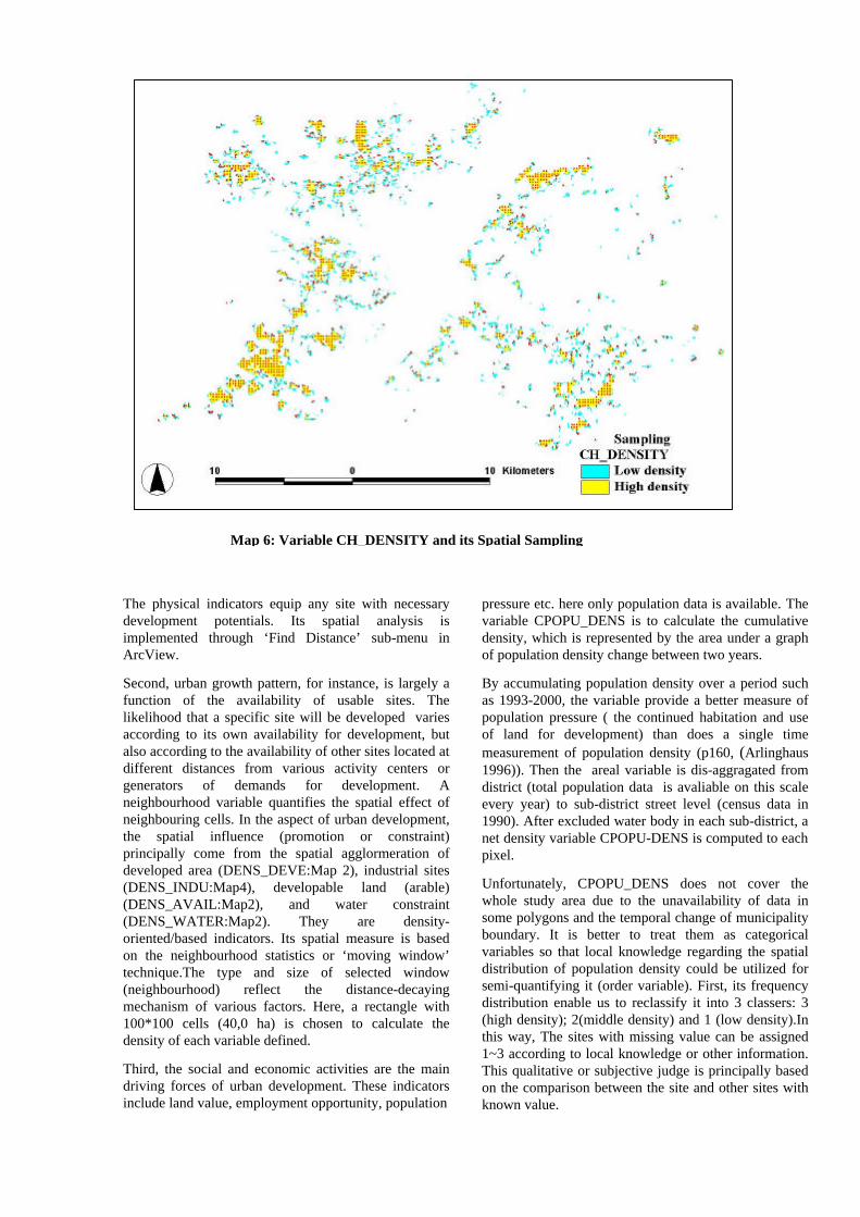
The physical indicators equip any site with necessary development potentials. Its spatial analysis is implemented through ‘Find Distance’ sub-menu in ArcView.

Second, urban growth pattern, for instance, is largely a function of the availability of usable sites. The likelihood that a specific site will be developed varies according to its own availability for development, but also according to the availability of other sites located at different distances from various activity centers or generators of demands for development. A neighbourhood variable quantifies the spatial effect of neighbouring cells. In the aspect of urban development, the spatial influence (promotion or constraint) principally come from the spatial agglormeration of developed area (DENS_DEVE:Map 2), industrial sites (DENS_INDU:Map4), developable land (arable) (DENS_AVAIL:Map2), and water constraint (DENS_WATER:Map2). They are density-oriented/based indicators. Its spatial measure is based on the neighbourhood statistics or ‘moving window’ technique.The type and size of selected window (neighbourhood) reflect the distance-decaying mechanism of various factors. Here, a rectangle with 100*100 cells (40,0 ha) is chosen to calculate the density of each variable defined.

Third, the social and economic activities are the main driving forces of urban development. These indicators include land value, employment opportunity, population

pressure etc. here only population data is available. The variable CPOPU_DENS is to calculate the cumulative density, which is represented by the area under a graph of population density change between two years.

By accumulating population density over a period such as 1993-2000, the variable provide a better measure of population pressure ( the continued habitation and use of land for development) than does a single time measurement of population density (p160, (Arlinghaus 1996)). Then the areal variable is dis-aggragated from district (total population data is avaliable on this scale every year) to sub-district street level (census data in 1990). After excluded water body in each sub-district, a net density variable CPOPU-DENS is computed to each pixel.

Unfortunately, CPOPU_DENS does not cover the whole study area due to the unavailability of data in some polygons and the temporal change of municipality boundary. It is better to treat them as categorical variables so that local knowledge regarding the spatial distribution of population density could be utilized for semi-quantifying it (order variable). First, its frequency distribution enable us to reclassify it into 3 classers: 3 (high density); 2(middle density) and 1 (low density).In this way, The sites with missing value can be assigned 1~3 according to local knowledge or other information. This qualitative or subjective judge is principally based on the comparison between the site and other sites with known value.

Map 6: Variable CH_DENSITY and its Spatial Sampling

Urban development is under the control of master planning and municipal administration management on macro level, which are generalized as macro policy

variables. Wether a site is planned as built-up or un- developable area (PLAN_NO) will essentially decide its change possibility. Wether a site is within the

adminstration of sub-district or others such as town, township and farms (STREET_NO) is also influencing its development scale and speed in a specific period. The spatial distribution of three variables (STREET_NO, PLAN_NO and CPOPU_DENS) can be seen from map 4.

Table 1: Variables and their descriptions Variables Descriptive Dependent Variable CHANGE (macro level) CH_DENSITY (meso level)

Binary variable, 1-change from rural to urban; no-change. Binary variable, 1- high density; 0 – low density.

Proximity Variables DIST_RAIL DIST_CENT DIST_MRD DIST_ORD DIST_RIVER DIST_PBRID DIST_CBRID

countinuous variable, distance to railway lines; countinuous variable, distance to city center/sub-centers; countinuous variable, distance to main roads; countinuous variable, distance to other roads except main roads; countinuous variable, distance to Yangtze/Han rivers; countinuous variable, distance to planned bridges; countinuous variable, distance to constructed bridges.

Neighbourhood Variables DENS_WATER DENS_DEVE DENS_INDU DENS_AVAIL

countinuous variable, desity of neighbouring waters ; countinuous variable, density of neighbouring areas developed; countinuous variable, density of neighbouring industrial areas; countinuous variable, density of neighbouring developable areas;

Nominal Variables PLAN_NO STREET_NO CPOPU_DENS

Binary variable, 1-planned as built-up area; 0-not; Binary variable, 1-sub-district; 0-not (town, township and farm); Order variable, 3~1 (high, middle and low density)

4. SOME FINDINGS

The real power of GIS resides in their display facilities; they still lack on the facility to visually explore relationships between multivariate data. Graphical representation of spatial relationships is generally more easily interpreted than numerical output. Towards this direction, exploratory spatial data analysis (ESDA) techniques are used to examine data for accuracy and robustness, detect spatial patterns in data, and to suggest hypothesis which may be tested in a later confirmatory stage (pre-modelling exploration). The techniques can also be used for examining model accuracy and robustness (post-modelling exploration). In modelling pattern, it has been receiving more and more attentions(Goodchild 2000) (Bell, Dean et al. 2000; Brunsdon 2001).

4.1 Change patterns detection

Comparing different maps and their pattern similarity using heuristic methods and simple statistics (such as mean, standard deviation, skewness, kurtosis, normality test) is one of the more promising approaches in understanding cumulative process-pattern relations (Gumbricht 1996). Their graphic representation can be Q-Q plot, Box-plot or Histogram graph and Moran scatterplot. The simple descriptive analyses are helpful in explaining the spatial distribution of variables studied, and suggest in this case that most continuous variables in table do not follow the normal distribution and have highly considerable amount of spatial outliers; however, these statistics are not able to compare/explain the spatial influences of each variable on urban growth, which is the general objective of this paper. Towards this exploration, this research proposes a simple

Distance to Centers/Sub_centers (m)

-12

-10

-8

-6

-4

-2

0

2

4

6

-2000 2000 6000 10000 14000 18000 22000

DIST_CENT Y=Log(p) DIST_CENT Y=Log(p/q)

Distance to Main Roads (m)

-12

-10

-8

-6

-4

-2

0

2

4

-2000 2000 6000 10000 14000 18000 22000

DIST_MRD Y=Log(p)DIST_MRD Y=Log(p/q)

Distance to Rivers (m)

-4

-3

-2

-1

0

1

2

-2000 2000 6000 10000 14000 18000 22000

DIST_RIVER Y=Log(p)DIST_RIVER Y=Log(p/q)

Distance to Railway Lines (m)

-14

-12

-10

-8

-6

-4

-2

0

2

-2000 2000 6000 10000 14000 18000 22000

DIST_RAIL Y=Log(p)DIST_RAIL Y=Log(p/q)

Distance to Other Roads (m)

-14

-12

-10

-8

-6

-4

-2

0

2

-2000 2000 6000 10000 14000 18000 22000

DIST_ORD Y=Log(p)DIST_ORD Y=Log(p/q)

Distance to Contructed Bridges (m)

-6

-4

-2

0

2

4

-2000 2000 6000 10000 14000 18000 22000

DIST_CBRID Y=Log(p)DIST_CBRID Y=Log(p/q)

Distance to Planned Bridges (m)

-7

-5

-3

-1

1

3

-2000 2000 6000 10000 14000 18000 22000

DIST_PBRID Y=Log(p)DIST_PBRID Y=Log(p/q)

Density

-10

-8

-6

-4

-2

0

2

4

6

-0.1 0.1 0.3 0.5 0.7 0.9 1.1

DENS_DEVE Y=Log(p)DENS_DEVE Y=Log(p/q)

Density

-9

-7

-5

-3

-1

1

-0.1 0.1 0.3 0.5 0.7 0.9 1.1

DENS_WATER Y=Log(p)DENS_WATER Y=Log(p/q)

Density

-6

-5

-4

-3

-2

-1

0

1

2

3

-0.1 0.1 0.3 0.5 0.7 0.9 1.1

DENS_AVAI Y=Log(p)DENS_AVAI Y=Log(p/q)

Density

-14

-12

-10

-8

-6

-4

-2

0

2

4

-0.1 0.1 0.3 0.5 0.7 0.9 1.1

DENS_INDU Y=Log(p)DENS_INDU Y=Log(p/q)

Distance to Rivers ( m)

-3.5

-3.0

-2.5

-2.0

-1.5

-1.0

-0.5

0.0

0.5

1.0

0 400 800 1200 1600 2000 2400

DIST_RIVER Y=Log(p/q) x < 2400 m

Figure 2: Scatter plots of Change Patterns Detection

method of pattern detection, defined as follows:

yi = f (xi)

Here, xi represents a discretion or partition of proximity space (proximity-based variable x, like the distance to main roads DIST_MRD), i.e. spatial partition with equal distance interval, such as 200 m interval. xi means the ith interval, for instance, x2=[200m~400m];

Change probability: yi=loge(pi/qi)

Change density: yi=loge(pi)

pi=Chi/? Chi

qi=NChi/? NChi

Chi and NChi indicate the total quantity of change (value 1) and no-change (value 0) located in xi

respectively. So pi represents the probability of urban growth and qi represents the probability of no growth, occurring in the spatial extent xi.

The dependent variable yi is defined as the logarithmic transformation of the ratio pi/qi for detecting change probability and the logarithm transformation of only pi

for detecting change density respectively as the histogram of most variables shows negative exponential distributions. In the case of change density, theoretically, Y is able to quantify the contribution or relative importance of x to urban growth through a series of xi, the greater yi is, the more contribution it makes. The spatial relationship can be visualized for pattern detect and hypothesis formation by using scatter plot (xi, yi).Further, a quantitative relationship between y and x, to some extent, represents the GLOBAL spatial influence of proximity variable on urban growth. In simplicity, supposed that a linear trend (in most cases) exists between yi and xi:

Y(d*)= a + b x

And xi<= d*; x1 < d*< maximum (xi),

Then, the slope b indicates the degree of spatial influences; b >0 means the positive influence; b<0 indicates the positive effect. The correlation coefficients R of linear equation indicates its accuracy or reliability of equation. As indicated in figure 2, parameter estimation of the linear equation depends on the scale of x, which is represented as d*. The spatial variability of equation y(d*) reflects the multi-scale and local feature of spatial influences, which also could be utilized for accuracy test of logistic regression modelling and evaluation of spatial sampling scheme.

For neighbourhood variable, xi represents a discretion/partition of density space such as DENS_DEVE (from 0 to 1), i.e. spatial partition with

equal density interval, such as 0.02 interval. xi means the ith interval, for instance, x2=[0.02~0.04].

In the case of Wuhan City, the interval of distance is 200m, equal to 10 pixels, and the interval of density is set as 0.02 correspondingly. The scatter plots of all continuous variables are shown in figure2, from which the global and local relationship, spatial outlier are easy to be detected. The figures may visually suggest an interesting table 2 (see below).

Table 2 suggests some significant differences between two scales. It should be noticed that the variables, which are not significant globally, may be strongly significant locally. For example, DIST_RIVER Y(2000 m) (see figure 2-12) exhibit strong positive influence locally. This spatial variability may influence parameter estimation of logistic regression modelling when spatial sampling is located in the d* extent.

The variables accepted above, together with 3 categorical variables (STREET_NO, PLAN_NO, CPOP_DENS), are further confirmed by using T-test (continuous type) and Chi-square test (norminal). Except PLAN_NO in change density, the rest are all statistically significant.

4.2 Logistic regression modelling

The exploratory data analysis in 4.1 help to hypothesize the spatial effects of each independent variable on change pattern but the analysis is not able to systamically compare their relative importances or contributions. Towards this objective, as argured before, this research applys logistic regression method integrated with spatial statistics. The general form of logistic regression can be described as follows:

Y = a + b1 x1+ b2 x2+...+bm xm

Y = loge (p / (1-p)) = logit (p)

Prob (z=1 ) = p = exp (y) / (1 + exp (y) )

Here x1, x2,,x3,..., xm are the explanatory variables describing the characteristics of development unit sampled. Y is a linear combination function of the explanatory variables, representing a linear relationship. The parameter b1, b2,..., bm are the regression coefficients to be estimated. If we denote Z as a binary response variable, vaule 1 (Z=1) means the occurence of new unit such as land use change from rural to urban, oppsitely, value 0 (Z=0) indicates no change. The P means the probability of occurence of new unit ie. Z=1. Function y is represented as logit(p), ie. the log (to base e) of the odds or likelihood ratio that the dependent variable Z is 1. Apparently, the probability can be a non-linear function of explanatory variables. This is a strictly increasing function, Propability p will increase with value y. Regression coefficients b1~bm imply the

contribution of each independent variable on propbability value p. A positive sign means that the independent variable will help to increase the probability of change and a negative sign has the opposite effect. From the perspective of statistics, logistic regression not only has strong interpretation

capacity (Koutsias and Karteris 2000) but also has other advantages, which is listed in table 3.Especially, its advantages in three aspects (dependent variable, independent variable and normality assumption) makes it best suitable for explanatory and confirmatory data analysis in this research.

Table 2: Comparisons of Changes pattern detect on two scales Change probability Change density

Variables

Significance R Outlier Significance R Outlier

Difference

DIST_RAIL - -0.79 y - -0.88 y DIST_CENT - -0.92 - -0.90 y DIST_MRD - -0.93 - -0.95 DIST_ORD - -0.87 - -0.91 DIST_RIVER # # -0.68 DIST_PBRID # # DIST_CBRID - -0.88 # Y DENS_WATER - -0.61 y - -0.97 DENS_DEVE + 0.856 - -0.87 Y DENS_INDU # - -0.96 Y DENS_AVAIL - -0.73 y - -0.68 y PLAN_NO # Y STREET_NO # Y CPOPU_DENS Y

#: not significant; +: positive; -: negative; y: outlier; Y: different on two scales; R: regression coefficients

However, the traditional application does not take spatial dependence into account, such as logistic regression modelling in (Tang and Choy 2000), (Wu 2000),(Wu and Yeh 1997). There are few selective alternatives to consider spatial dependence. one is to build a more complex model containing an autogressive structure like (Gumpertz, Wu et al. 2000). Another is to design a spatial sampling scheme to expand the distance interval between the sampled sites. The latter results in a much smaller size of sample, which will lose certain information. However, the maximum likelihood method, upon which logistic regression is based, relies on large-sample of asymptotic normality, it means the result may not be reliable when the sample size is small. Consequently, a conflict occurs in applying logistic regression: removal of spatial dependence and large size of sample, a reasonable design of spatial sampling scheme is becoming a crucial point of spatial statistics, which has attracted more and more researchers in various areas (Stehman and Overton 1996).

Frequently adopted schemes in logistic regression modelling are either stratified random sampling (Atkinson and Massari 1998; Dhakal, Amada et al. 2000; Gobin, Campling et al. 2001) or systematic sampling (Ville and al ; Pereira and Itami 1991; Sikder 2000). Their advantages and drawbacks were detailly reviewed and compared by (Stehman and Overton 1996). Unlike the spatial prediction purpose in the area of geostatistics, the population studied here is completely known, spatial sampling aims to reduce

the size of samples (the population is around 17,00000 pixels, which is beyond the capacities of most statistical softwares) and remove spatial auto-correlation. Systematic sampling is effective to better reduce spatial dependence but it may lose some important information like relatively isolated sites when population is spatially not homogenuous. Especially, its representativity of population may decreases when distance interval increases significantly. Conversely, random sampling is efficient to represent population but low efficient to reduce spatial dependence especially local spatial dependence. It should be noted that some independent variables like the distance to roads are in essence strong in spatial trendness. Hense, it cannot be expected to absolutely remove it. Following the idea, we are able to integrate systematic and random sampling to balance sample size and spatial dependence.

Spatial sampling on change probability level

First, a systematic sampling is implemented for whole the population studied.When a 12th order lag (12 pixels or 240 m in east-west and north-south directions) is reached, Moran’ I index drops from 0.83-0.93 to 0.50-0.73 for all continuous independent variables. The original ratio of two value 1 & 0 (dependent variable) is about 1:10 (156561:1506473 based on 20 *20 m2 grid). After systematic sampling, the ratio is changed to 1:12 (1034: 12000). To gain an unbiased parameter estimation, we continue to randomly select 12% of sample 0 in order to obstain

an equal size for both 1 and 0. This random sampling is able to create a 1034: 1143 map (see map 4 ). Experimentally, that is the limit of large sample size in relation to total 13 mixtured variables (there are at

least 10 trials at each combination of X variables value). The systematic and random sampling are implemented by the spatial module of ArcInfo 8.0.

Table 3: Comparison of main regression techniques for modeling urban development

Type of regression

Dependent variable

Independent variable

Computation method

Normality assumption

Multi collinearity

Relationship

Multivariate regression

Continuous Only continuous

OLS Yes yes linear

Log-linear regression

Categorical Only Categorical

GLS No yes Non-linear

Logistic regression

Binary nominal

mixture GLS No yes Non-linear

GLS: Generalized Least Square, OLS: Ordinary Least Square

Spatial sampling on change density level

First, for high-density class (1), a systematic sampling is implemented with a 10th order. the original sample is reduced to 770 from 77752. For low-density class (0), around 1% random sampling from original size (78809) is able to obstain nearly an equal size of sample (see Map 6). For total size of sample (1549), Moran’ I index drops from 0.89-0.97 to 0.61-0.76 for all continuous independent variables. Regarding multi-collinearity, Subsequently, of all pairs of variables

with a correlation over 0.80, one is omitted. Of all pairs of variables with a correlation over 0.50, only one is allowed to enter a regression equation. The use of a stepwise regression procedure solves remaining multi-collinearity problems. A forward stepwise variable selection is employed via SPSS package. After 8 and 10 steps (the significance evel for entry is 0.1, for removal is 0.2, the classification cutoff is 0.5), the results were calculated seperately as listed in table 4.

Table 4: logistic regression results on two scales Variables Change probability Change density Steps of regression 8 10 Sample size 2256 1549 Co-efficients B (SE, Wald) B (SE, Wald) DIST_CBRID -2.923 (0.69, 18.2) * # DIST_CENT -1.859 (0.68, 7.5) * -1.254 (0.5, 6.316) * DIST_MRD -5.409 (0.64, 70.5) * -1.757 (0.37, 22.6) * DIST_ORD -16.922 (1.7 , 96.2) * -2.223 (0.58, 15) * DIST_RAIL 1.349 (0.51, 6.87) * # DENS_AVI # 0.183 (0.078, 5.450) 0.02 DENS_INDU # -0.078 (0.032, 5.943)* DENS_DEVE # -0.095 (0.04, 6.13) * DENS_WATER -0.196 (0.04, 21.85) * -0.04 (0.034, 5.9) * PLANNO(1) -0.649 (0.13, 26.9) * # STREETNO(1) # 0.644 (0.162, 15.9) * CPOPDENS (1) 1.640 (0.63, 6.8) * -2.55 (1.1, 5.4) 0.02 CPOPDENS (2) 2.184 (0.71, 9.6) * -2.7 (1.08, 6.26 ) * CONSTANT 2.841 (0.68, 17.2) * 3 (1.02, 8.6) * Tests -2 Log likelihood 1794.7 1983.6 Cox & Snell R Square 0.445 0.1 Nagelkerke R Square 0.593 0.134 Percentage of correct (PCP)

76.5% (0), 86% (1) 68.7%(0), 77.9%(1) 73.3%

*: p<0.01, #: Not selected or Rejected by step wise regression , SE: standard error.

4.3 Interpretation of results and the multi-scale issue

Logistic regression models are estimated by the maximum likelihood method. There are various ways to assess the goodness-of-fit of logistic regression. One way is to cross-tabulate prediction with observation and to calculate the percentage correctly predicted (PCP). Table 4 shows the estimated logistic regression models, the 2 models have their test significant at the 0.01 level. The overall percentage of correctness is about 80% for Change probability and 73% for change density. Sign ‘+” indicates a positive effect and ‘-‘ for negative influence.

On change probability scale: the main variables with strong negative effect are DIST_ORD, DIST_MRD, DIST_CBRID and DIST_CENT (the nearer it is to, the faster change it has). The weak negative variables are PLAN_NO and DENS_WATER. The variables with positive effects are DIST_RAIL and CPOPU_DENS.

On change density scale : the main variables with strong negative effect are DIST_ORD, DIST_MRD, DIST_CENT), and CPOPU_DENS (high and middle density). The weak negative variables are DENS_WATER, DENS_INDU and DENS_DEVE. However, STREET_NO and DENS_AVAI exhibit strong positive influence.

Comparing the spatial determinants on two scales, major changes are dominated by 6 variables (DIST_CBRID, DIST_RAIL, DENS_AVI, DENS_DEVE, DENS_INDU, and PLAN_NO). It implies that most factors , except roads (DIST_MRD, DIST_ORD), water (DENS_WATER) and centers (DIST_CENT), are scale-dependent. It indicates that relatively proximity variables like road infrastructure city center/sub-center and water body have scale-independent influences (positive or negative) on urban development.

The result from logistic regression modelling is basically consistent with that of change pattern detection (see table 2). Therefore, The latter to some extent confirms the reliability of the former.

5. DISCUSSION

The partial results from only two scales have shown that a multi-scale property exists in urban development pattern modelling, which is quite different from data resolution. The distinguishing determinants on various scales are helpful to strengthen deep insights into urban development processes. Of course, we need to study another micro scale for modelling change intensity. On this micro scale, the analysis may undergo major changes. First of all, proximity-based variables may not reflect the spatial effects of

infrastructure and public facilities on urban redevelopment, accessibility-based measure may better model it. Second, the primary data sources could be IKONOS with 1m resolution or aerial photos, which is able to extract two levels of redevelopment (1: higher buildings; 0: lower buildings). Third, the neighbouring land use and detailed control plan may be also highly important factors. The outcome on this scale can be utilized for systematic comparisons of multi-extent data analysis. In the future, the multi-scale framework of pattern modelling is expected to link with multi-scale process modelling, such as cellular automata.

1) Scale and data resolution

The statistical property of neighborhood variable like DENS_DEVE largely depends on the type and especially size of neighborhood chosen. Over- or under-defined neighborhood will lead to highly skewed histogram, which makes analysis result unreliable. As a simply way, quite a few of tests with different choices have to be made for comparison, it is very time consuming and laborious. As a consequence, it is necessary to develop an algorithm for automatically seeking an optimal neighborhood, which is able to create approximately normal distribution.

The spatial analysis of this research is based on the resolution of 20*20 m2 grid as 10*10 m2 will create voluminous amount of data beyond the capacities of current hardware and software. The selection is corresponding to the resolution of SPOT images and also an ideal solution to solve the MAUP (Modifiable Area Unit Problem) issues as the lowest level (Wong 1996). However, other resolutions from 30*30 to 100*100 m2 need to be comparatively checked for the sensitivity analysis of logistic regression modelling results. The change pattern detection is based on the distance interval of 200 m, a test with 100m and 300 m confirm the stability of analysis result.

2) Spatial auto-correlation and sampling

Unlike natural science, urban development like other social sciences is in essence not a completely random or stochastic process. The proximity-based and neighborhood-based variables are created just according to spatial dependence or we can say that spatial proximity is one way of spatial dependence. Consequently, complete removal of spatial dependence is impossible. A feasible way is to compare various sampling schemes for a compromised alternative according to current development and techniques of spatial statistics. An ideal scheme should satisfy the following conditions:

?? Make the spatial auto-correlation index of all variables as small as possible;

?? Have a sample size enough for maximum likelihood modeling;

?? Represent the distribution of known population.

This is a global spatial optimization issue. Groenigen (1998) already explored the case of uni-variate by applying spatial simulated annealing algorithm in the area of soil sampling. Further research is needed more advances in simulated annealing, genetic algorithms etc. 3) Spatial data analysis

This research also found that logistic regression analysis is very sensitive to its assumptions such as data transformation, spatial sampling. The logarithm data transformation LN(y +?) (? is to be determined by experiments) and various combination of sampling type and size may significantly influence parameter estimation and model accuracy. The selection or design of reasonable data transformation and spatial sampling still need further systematic research for logistic regression modelling. Spatial exploratory data analysis, like a simple detect method proposed in this paper, is quite helpful for testing the detected pattern with the outcome of logistic regression. Exploratory spatial data analysis is able to discover the influence of each continuous variable but not systematic ranking. Logistic regression is efficient in systematically evaluating their relative contribution. Consequently, the integration of both is a feasible way for hypothesis formation and the test of model accuracy.

Acknowledgement

Without financial support and facilities, this study could not be successfully completed. We would like to thank DSO project between ITC-SUS (SUS: School of Urban Studies, Wuhan University, P.R.China). The research also needs considerable data support including primary and secondary data sources. Without them, any perfect methodology would be an empty page and never be fulfilled. We would also like to thank all persons who assisted this research in data collection during the fieldwork in Wuhan.

REFERENCES

Arlinghaus, S. L. (1996). Practical Handbook of Spatial Statistica, CRC Press.

Atkinson, P. M. and R. Massari (1998). “Generalised Linear Modelling of Susceptibility to Landslide in the Central Apennines, Italy.” Computers and Geosciences 24(4): 373-385.

Bell, M., C. Dean, et al. (2000). “Forecasting the pattern of urban growth with PUP: a web-based model interfaced with GIS and 3D animation.” Computers, Environment and Urban Systems 24: 559-581.

Brunsdon, C. (2001). “The comap: exploring spatial pattern via conditional distributions.” Computers, Environment and Urban Systems 25: 53-68.

Cheng, J., J. Turkstra, et al. (2001). "The Changing Urban Fabric of Chinese Cities, Wuhan 1955-2000". Urban Geoinformatics, Wuhan, P.R.China, Wuhan University.

Chuvieco, E. (1999). “Measuring changes in landscape pattern from satellite images:short-term effects of fire on spatial diversity.” Int. J. Remote Sensing 20(12): 2331-2346.

Currit, N. (2000). An inductive attack on spatial scale. Geocomputation'2000, University of Greenwich, UK.

Desyllas, J., G. M., et al. (1997). "The Spatial Configuration of a Rapidly Growing City; Implications on the Quality of Urban Life". 5th International Conference on Computers in Urban Planning and Urban Management, Mumbai, India.

Dhakal, A. S., T. Amada, et al. (2000). “Landslide Hazard Mapping and Its Evaluation using GIS: An Investigation of Sampling Schemes for a Grid-Cell Based Quantitative Method.” Photogrammetric Engineering and Remote Sensing 66(8): 981-989.

Gao, J. and D. Skillcorn (1998). “Capabil ity of SPOT XS data in producing detailed land cover maps at the urban-rural periphery.” Int. J. Remote Sensing 19(15): 2877 - 2891.

Gaubatz, P. (1999). “China's urban transformation: patterns and process of morphological change in Beijing, shanghai and Guangzhou.” Urban Studies 36(9): 1495-1521.

Gobin, A., P. Campling, et al. (2001). “Spatial Analysis of Rural Land ownership.” Landscape and Urban Planning 55: 185-194.

Goodchild, M. F. (2000). "Spatial Analysis: Methods and Problems in Land Use Management". Spatial Information for Land Use Management. M. J. Hill and R. J. Aspinall. Singapore, Gordon and Breach Science Publishers: 39-50.

Gumbricht, T. (1996). "Landscape interfaces and transparency to hydrological functions". HydroGIS'96: Application of GIS in Hydrology and Water Resources Management, IAHS Publ. No: 235.

Gumpertz, M. L., C.-t. Wu, et al. (2000). “Logistic regression for Southern pine beetle outbreaks with spatial and temporal autocorrelation.” Forest Science 46(1): 95-107.

Irwin, E. G. and J. Geoghegan (2001). “Theory, data, methods: developing spatially explicit economic models of land use change.” Agriculture, Ecosystems and Environment 85: 7-23.

Jensen, J. R. (1996). Introductory Digital Image Processing. A Remote Sensing Perspective 2nd edn. New Jersey:, Prentice-Hall.

Jiang, B., C. Claramunt, et al. (1999). “Geometric accessibility and geographic information: extending

desktop GIS to space syntax.” Computer, Environment and Urban Systems 23: 127-146.

Kivell, P. (1993). LAND and the CITY pattern and process of urban change, Routledge.

Kok, K. and A. Veldkamp (2001). “Evaluating impact of spatial scales on land use pattern analysis in Central America.” Agriculture, Ecosystems and Environment 85: 205-221.

Koutsias, N. and M. Karteris (2000). “Burned area mapping using logistic regression modeling of a singlepost-fire Landsat-5 Thematic Mapper image.” Int. J. Remote Sensing 21(4): 673-687.

Makse, H. A., J. S. Andrade, et al. (1998). “Modelling urban growth patterns with Correlated Percolation.” Physics Review. E 58(6): 7054-7062.

Morisette, J. T., S. Khorram, et al. (1999). “Land-cover change detection enhanced with generalized linear models.” INT.J.Remote Sensing 20(14): 2703-2721.

Pereira, J. M. C. and R. M. Itami (1991). “GIS-based habitat modelling using logistic multiple regression: a study of the Mt.Graham red squirrel.” Photogrammetric Engineering and Remote Sensing 57(11): 1475-1486.

Quarmby, N. A. and J. L. Cushnie (1989). “Monitoring urban land cover changes at the urban fringe from SPOTHRV imagery in south-east England.” International Journal of Remote Sensing 10: 953-963.

Rodrigue, J. P. (1997). “Parallel modelling and neural networks: an overview for transportatio/land use systems.” Transportation Research Part C 5(5): 259-271.

Schneider, L. C. and R. Gil Pontius Jr. (2001). “Modeling land-use change in the Ipswich watershed, Massachusetts, USA.” Agriculture, Ecosystems and Environment 85: 83-94.

Serneels, S. and E. F. Lambin (2001). “Proximate causes of land-use change in Narok District, Kenya: a spatial statistical model.” Agricultural Ecosystem and Environment 85: 65-81.

Shen, G. (1997). “A fractal dimension analysis of urban transportation networks.” Geographical and Environmental Modelling 1(2): 221-236.

Sikder, I. U. (2000). “Land Cover Madelling: A Spatial Statistical Approach.” Geoinformatics: Beyond 2000: An international conference on Geoinformatics for natural resource assessment, monitoring and management, IIRS, Dehradun, India: 294-308.

Stanilov, K. (1998). Urban growth, land use change, and metropolitan restructuring: the case of greater seattle, 1960-1990 (Washionton), University of Washington: 375.

Stehman, S. V. and W. S. Overton (1996). Spatial Sampling. Practical Handbook of Spatial Statistics. S. L. Arlinghaus, CRC Press: 31-64.

Tang, B.-S. and L. H.-T. Choy (2000). “Modelling planning control decisions: a logistic regression analysis on office development applications in urban Kowloon, Hong Kong.” Cities 17(3): 219–225,.

Terrettaz, P. (1998). Comparison of different methods to merge SPOT T and XS data: evaluation in an urban area. Future trends in remote sensing. Gudmandsen. Rotterdam, Malkema.

Ville, N. D. L. and et. al. (1999)."Habitat suitability analysis using logistic regression and GIS to outline potential areas for conservation of grey wolf (canis lupus)": 187-197.

Walsh, S. J. and T. W. Crawford (2001). “A multiscale analysis of LULC and NDVI variation in Nang Rong district, northeast Thailand.” Agriculture, Ecosystems and Environment 85: 47-64.

Wong, D. (1996). Aggregation Effects in Geo-referenced Data. Practical Handbook of Spatial Statistics. S. L. Arlinghaus, CRC Press: 83-106.

Wu, F. (1998). “The new structure of building provision and the transformation of the urban landscape in metropolitan Guangzhou, China.” Urban Studies 35(2): 259-283.

Wu, F. (2000). “Modelling Intrametropolitan Location of Foreign Investment Firms in a Chinese City.” Urban Studies 37(13): 2441– 2464.

Wu, F. and A. G.-O. Yeh (1997). “Changing spatial distribution and determinants of land development in Chinese cities in the transition from a centrally planned economy to a socialist market economy: a case study of Guangzhou.” Urban Studies 34(11): 1851-1879.