arX

iv:1

711.

1098

0v1

[qu

ant-

ph]

29

Nov

201

7

Toward the first quantum simulation with quantum speedup

Andrew M. Childs,1,2,3,∗ Dmitri Maslov,2,3,4 Yunseong Nam2,3,5,

Neil J. Ross2,3,6, and Yuan Su1,2,3

1Department of Computer Science, University of Maryland2Institute for Advanced Computer Studies, University of Maryland

3Joint Center for Quantum Information and Computer Science, University of Maryland4National Science Foundation

5IonQ, Inc.6Department of Mathematics and Statistics, Dalhousie University

Abstract

With quantum computers of significant size now on the horizon, we should understand howto best exploit their initially limited abilities. To this end, we aim to identify a practical problemthat is beyond the reach of current classical computers, but that requires the fewest resourcesfor a quantum computer. We consider quantum simulation of spin systems, which could beapplied to understand condensed matter phenomena. We synthesize explicit circuits for threeleading quantum simulation algorithms, employing diverse techniques to tighten error boundsand optimize circuit implementations. Quantum signal processing appears to be preferred amongalgorithms with rigorous performance guarantees, whereas higher-order product formulas prevailif empirical error estimates suffice. Our circuits are orders of magnitude smaller than those forthe simplest classically-infeasible instances of factoring and quantum chemistry.

1 Introduction

While a scalable quantum computer remains a long-term goal, recent experimental progress suggeststhat devices capable of outperforming classical computers will soon be available [10, 21, 28, 38, 73,78]. Multiple groups have already developed programmable devices with several qubits and two-qubit gate fidelities around 98% [49], and similar devices with around 50 qubits are under activedevelopment. While the error rates of these early machines severely limit the total number of gatesthat can be reliably performed, future improvements should lead to machines with more qubits andmore reliable gates. This raises the exciting possibility of solving practical problems that are beyondthe reach of classical computation. Such an outcome would be a landmark in the development ofquantum computers and would begin an era in which they serve not only as testbeds for science,but as practical computing machines.

Reaching this goal will require not only significant experimental advances, but also careful quan-tum algorithm design and implementation. Here we address the latter issue by developing explicitcircuits, and thereby producing concrete resource estimates, for practical quantum computationsthat can outperform classical computers. Through this work, we aim to identify applications forsmall quantum computers that help to motivate the significant investment required to developscalable, fault-tolerant quantum computers.

There has been considerable previous research on compiling quantum algorithms into explicitcircuits (see Appendix A for more detail). However, to the best of our knowledge, none of these

1

studies aimed to identify minimal examples of super-classical quantum computation, and typicalresource counts were high. Our work is also distinct from recent work on quantum computationalsupremacy [35], where the goal is merely to accomplish a super-classical task, regardless of itspracticality. Instead, we aim to pave the way toward practical quantum computations (which maynot be far beyond the threshold for supremacy).

Arguably, the most natural application of quantum computers is to the problem of simulatingquantum dynamics [30]. Quantum computers can simulate a wide variety of quantum systems,including fermionic lattice models [77], quantum chemistry [76], and quantum field theories [40].However, simulations of spin systems with local interactions likely have less overhead, so we focuson them as an early candidate for practical quantum simulation. While analog simulation may beeasier to realize in the short term, we focus on digital simulation for its greater flexibility and theprospect of invoking fault tolerance.

Efficient quantum algorithms for simulating quantum dynamics have been known for over twodecades [50]. Recent work has led to algorithms with significantly improved asymptotic performanceas a function of various parameters such as the evolution time and the allowed simulation error[11, 12, 14, 51, 52]. Our work investigates whether these alternative algorithms can be advantageousfor simulations of relatively small systems, and aims to lay the groundwork for the first practicalapplication of quantum computers.

2 Target system

To produce concrete benchmarks, we focus on a specific simulation task. Specifically, we consider aone-dimensional nearest-neighbor Heisenberg model with a random magnetic field in the z direction.This model is described by the Hamiltonian

n∑

j=1

(~σj · ~σj+1 + hjσzj ) (1)

where ~σj = (σxj , σyj , σ

zj ) denotes a vector of Pauli x, y, and z matrices on qubit j. We impose

periodic boundary conditions (i.e., ~σn+1 = ~σ1), and hj ∈ [−h, h] is chosen uniformly at random.The parameter h characterizes the strength of the disorder.

This Hamiltonian has been considered in recent studies of self-thermalization and many-bodylocalization (see Appendix B for more detail). Despite intensive investigation, the details of atransition between thermal and localized phases remain poorly understood. A major challenge isthe difficulty of simulating quantum systems with classical computers; indeed, the most extensivenumerical study we are aware of was restricted to at most 22 spins [54].

Hamiltonian simulation can efficiently access any feature that could be observed experimentally(and more), and there are several proposals for exploring self-thermalization by simulating dynamics[67, 68, 70]. Since all of these approaches involve only very simple state preparations and measure-ments, we focus on the cost of simulating dynamics. We consider evolution times comparable tothe number of spins, since the system must evolve for this long for self-thermalization to take place(or even for information to propagate across the system, owing to the Lieb-Robinson bound).

Specifically, we produce gate counts for simulations with h = 1, evolution time t = n (thenumber of spins in the system), and overall accuracy ǫ = 10−3. These explicit choices help us tofocus on the system-size dependence of quantum simulation algorithms. This is a key considerationfor practical applications, yet it has been deemphasized in the literature on sparse Hamiltoniansimulation.

2

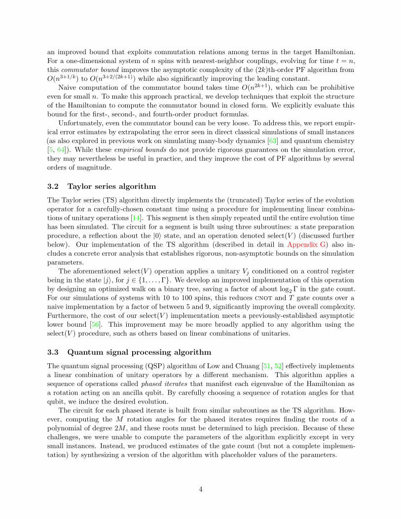
Algorithm Ref. Gate complexity (t, ǫ) Gate complexity (n)

Product formula (PF), 1st order [50] O(t2/ǫ) O(n5)

Product formula (PF), (2k)th order [11] O(52kt1+1/2k/ǫ1/2k) O(52kn3+1/k)

Quantum walk [12] O(t/√ǫ) O(n4 logn)

Fractional-query simulation [13] O(

t log2(t/ǫ)log log(t/ǫ)

)

O(

n4 log nlog logn

)

Taylor series (TS) [14] O(

t log2(t/ǫ)log log(t/ǫ)

)

O(

n3 log2 nlog logn

)

Linear combination of quantum walk steps [15] O(

t log3.5(t/ǫ)

log log(t/ǫ)

)

O(

n4 log nlog logn

)

Quantum signal processing (QSP) [51] O(t+ log(1/ǫ)) O(n3 logn)

Table 1: Previously-established asymptotic gate complexities of quantum simulation algorithms as a functionof the simulation time t, allowed error ǫ, and the system size n for a one-dimensional nearest-neighbor spinmodel as in (1) with t = n and fixed ǫ.

3 Implementations

There are many distinct quantum algorithms for Hamiltonian simulation, some of which are summa-rized in Table 1. We implement algorithms based on high-order product formulas (PF, introducedin Section C.1) [11], direct application of the Taylor series (TS, Section C.2) [14], and the recentquantum signal processing method (QSP, Section C.3) [51]. We expect these to be among the mostefficient approaches to digital quantum simulation. In particular, approaches based on quantumwalk [12, 15] appear to incur greater overhead (as discussed in Appendix D).

To produce concrete circuits, we implement quantum simulation algorithms in a quantum circuitdescription language called Quipper [32] (see Appendix E for more details). Wherever possible,we tighten the analysis of algorithm parameters and manually optimize the implementation. Wealso process all circuits using an automated tool we developed for large-scale quantum circuitoptimization [57]. Our implementation is available in a public repository [26].

We express our circuits over the set of two-qubit cnot gates, single-qubit Clifford gates, andsingle-qubit z rotations Rz(θ) := exp(−iσzθ/2) for θ ∈ R. Such gates can be directly implementedat the physical level with both trapped ions [28] and superconducting circuits [21, 38]. In bothtechnologies, two-qubit gates take longer to perform and incur more error than single-qubit gates.Thus, the cnot count is a useful figure of merit for assessing the cost of physical-level circuits ona universal device. We also produce Clifford+T circuits using optimal circuit synthesis [66] so thatwe can count T gates, which are typically the most expensive gates for fault-tolerant computation.

Our analysis ignores many practical details, such as architectural constraints, instead aimingto give a broad overview of potential implementation costs that can be refined for specific systems.When counting qubits, we assume that measured ancillas can be reused later.

3.1 Product formula algorithm

The product formula (PF) approach approximates the exponential of a sum of operators by aproduct of exponentials of the individual operators. The asymptotic complexity of this approachcan be improved with higher-order Suzuki formulas [74]. By splitting the evolution into r segmentsand making r sufficiently large, we can ensure that the simulation is arbitrarily precise. The mainchallenge in making these algorithms concrete is to choose an explicit r that ensures some desiredupper bound on the error. Appendix F gives a detailed description of these implementation details.

We present two bounds, which we call the analytic andminimized bounds, that slightly strengthenprevious analysis [11]. However, bounds of this type are far from tight [5, 63, 64]. Thus, we develop

3

an improved bound that exploits commutation relations among terms in the target Hamiltonian.For a one-dimensional system of n spins with nearest-neighbor couplings, evolving for time t = n,this commutator bound improves the asymptotic complexity of the (2k)th-order PF algorithm fromO(n3+1/k) to O(n3+2/(2k+1)) while also significantly improving the leading constant.

Naive computation of the commutator bound takes time O(n2k+1), which can be prohibitiveeven for small n. To make this approach practical, we develop techniques that exploit the structureof the Hamiltonian to compute the commutator bound in closed form. We explicitly evaluate thisbound for the first-, second-, and fourth-order product formulas.

Unfortunately, even the commutator bound can be very loose. To address this, we report empir-ical error estimates by extrapolating the error seen in direct classical simulations of small instances(as also explored in previous work on simulating many-body dynamics [63] and quantum chemistry[5, 64]). While these empirical bounds do not provide rigorous guarantees on the simulation error,they may nevertheless be useful in practice, and they improve the cost of PF algorithms by severalorders of magnitude.

3.2 Taylor series algorithm

The Taylor series (TS) algorithm directly implements the (truncated) Taylor series of the evolutionoperator for a carefully-chosen constant time using a procedure for implementing linear combina-tions of unitary operations [14]. This segment is then simply repeated until the entire evolution timehas been simulated. The circuit for a segment is built using three subroutines: a state preparationprocedure, a reflection about the |0〉 state, and an operation denoted select(V ) (discussed furtherbelow). Our implementation of the TS algorithm (described in detail in Appendix G) also in-cludes a concrete error analysis that establishes rigorous, non-asymptotic bounds on the simulationparameters.

The aforementioned select(V ) operation applies a unitary Vj conditioned on a control registerbeing in the state |j〉, for j ∈ {1, . . . ,Γ}. We develop an improved implementation of this operationby designing an optimized walk on a binary tree, saving a factor of about log2 Γ in the gate count.For our simulations of systems with 10 to 100 spins, this reduces cnot and T gate counts over anaive implementation by a factor of between 5 and 9, significantly improving the overall complexity.Furthermore, the cost of our select(V ) implementation meets a previously-established asymptoticlower bound [56]. This improvement may be more broadly applied to any algorithm using theselect(V ) procedure, such as others based on linear combinations of unitaries.

3.3 Quantum signal processing algorithm

The quantum signal processing (QSP) algorithm of Low and Chuang [51, 52] effectively implementsa linear combination of unitary operators by a different mechanism. This algorithm applies asequence of operations called phased iterates that manifest each eigenvalue of the Hamiltonian asa rotation acting on an ancilla qubit. By carefully choosing a sequence of rotation angles for thatqubit, we induce the desired evolution.

The circuit for each phased iterate is built from similar subroutines as the TS algorithm. How-ever, computing the M rotation angles for the phased iterates requires finding the roots of apolynomial of degree 2M , and these roots must be determined to high precision. Because of thesechallenges, we were unable to compute the parameters of the algorithm explicitly except in verysmall instances. Instead, we produced estimates of the gate count (but not a complete implemen-tation) by synthesizing a version of the algorithm with placeholder values of the parameters.

4

10 100

105

106

107

108

109

1010

20 30 50 70

System size

cnotgate

count

PF (com 4)

PF (emp)

TS

QSP (seg)

QSP (JA emp)

10 100

107

108

109

1010

1011

1012

20 30 50 70

System size

Tgate

count

PF (com 4)

PF (emp)

TS

QSP (seg)

QSP (JA emp)

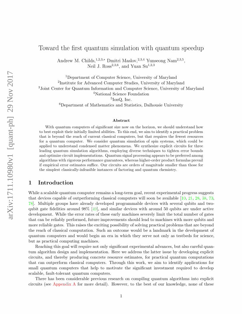
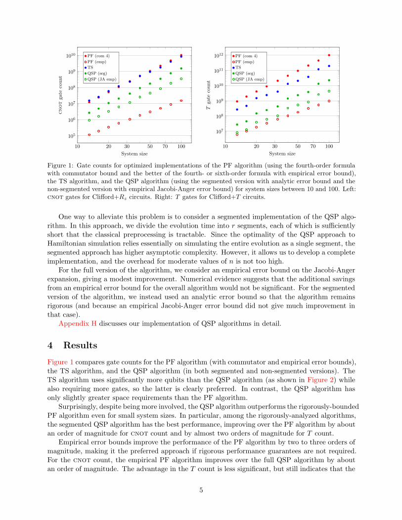
Figure 1: Gate counts for optimized implementations of the PF algorithm (using the fourth-order formulawith commutator bound and the better of the fourth- or sixth-order formula with empirical error bound),the TS algorithm, and the QSP algorithm (using the segmented version with analytic error bound and thenon-segmented version with empirical Jacobi-Anger error bound) for system sizes between 10 and 100. Left:cnot gates for Clifford+Rz circuits. Right: T gates for Clifford+T circuits.

One way to alleviate this problem is to consider a segmented implementation of the QSP algo-rithm. In this approach, we divide the evolution time into r segments, each of which is sufficientlyshort that the classical preprocessing is tractable. Since the optimality of the QSP approach toHamiltonian simulation relies essentially on simulating the entire evolution as a single segment, thesegmented approach has higher asymptotic complexity. However, it allows us to develop a completeimplementation, and the overhead for moderate values of n is not too high.

For the full version of the algorithm, we consider an empirical error bound on the Jacobi-Angerexpansion, giving a modest improvement. Numerical evidence suggests that the additional savingsfrom an empirical error bound for the overall algorithm would not be significant. For the segmentedversion of the algorithm, we instead used an analytic error bound so that the algorithm remainsrigorous (and because an empirical Jacobi-Anger error bound did not give much improvement inthat case).

Appendix H discusses our implementation of QSP algorithms in detail.

4 Results

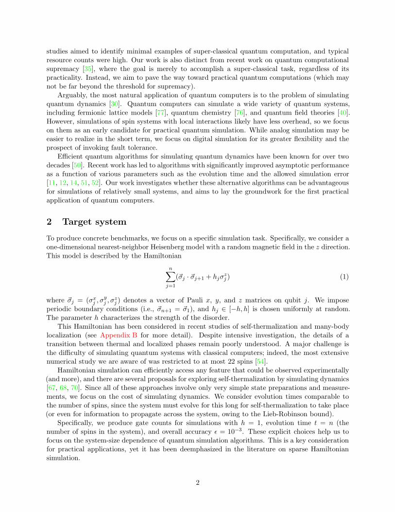
Figure 1 compares gate counts for the PF algorithm (with commutator and empirical error bounds),the TS algorithm, and the QSP algorithm (in both segmented and non-segmented versions). TheTS algorithm uses significantly more qubits than the QSP algorithm (as shown in Figure 2) whilealso requiring more gates, so the latter is clearly preferred. In contrast, the QSP algorithm hasonly slightly greater space requirements than the PF algorithm.

Surprisingly, despite being more involved, the QSP algorithm outperforms the rigorously-boundedPF algorithm even for small system sizes. In particular, among the rigorously-analyzed algorithms,the segmented QSP algorithm has the best performance, improving over the PF algorithm by aboutan order of magnitude for cnot count and by almost two orders of magnitude for T count.

Empirical error bounds improve the performance of the PF algorithm by two to three orders ofmagnitude, making it the preferred approach if rigorous performance guarantees are not required.For the cnot count, the empirical PF algorithm improves over the full QSP algorithm by aboutan order of magnitude. The advantage in the T count is less significant, but still indicates that the

5

0 20 40 60 80 100

0

50

100

150

200

250

System size

Qubits

PFTSQSP

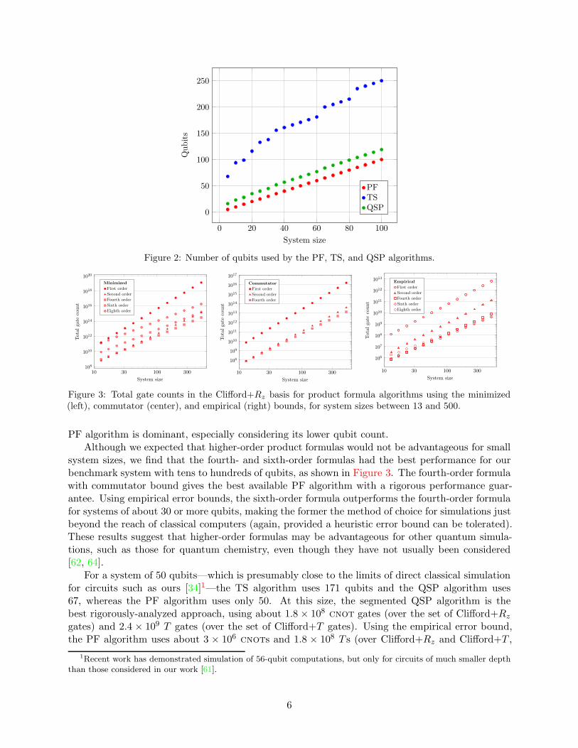
Figure 2: Number of qubits used by the PF, TS, and QSP algorithms.

10 100108

1010

1012

1014

1016

1018

1020

30 300

System size

Total

gate

count

Minimized

First order

Second order

Fourth order

Sixth order

Eighth order

10 100

108

109

1010

1011

1012

1013

1014

1015

1016

1017

30 300

System size

Total

gate

count

Commutator

First order

Second order

Fourth order

10 100

106

107

108

109

1010

1011

1012

1013

30 300

System size

Total

gate

count

Empirical

First order

Second order

Fourth order

Sixth order

Eighth order

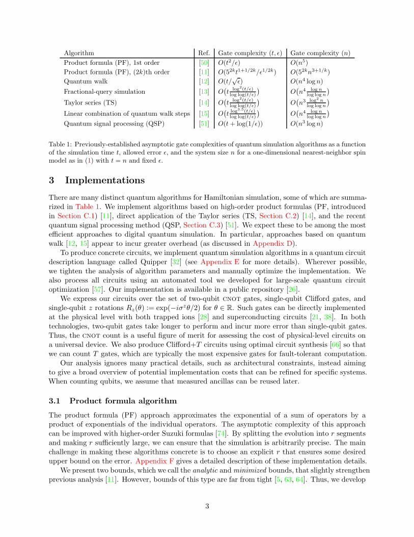
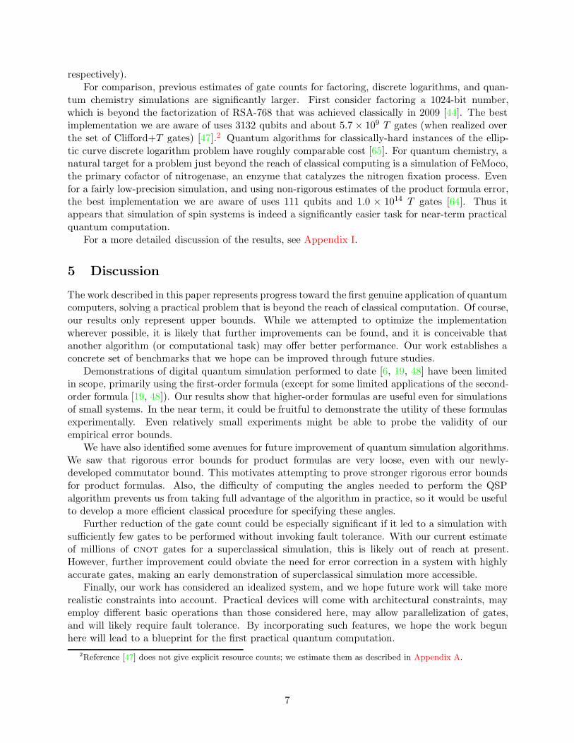
Figure 3: Total gate counts in the Clifford+Rz basis for product formula algorithms using the minimized(left), commutator (center), and empirical (right) bounds, for system sizes between 13 and 500.

PF algorithm is dominant, especially considering its lower qubit count.Although we expected that higher-order product formulas would not be advantageous for small

system sizes, we find that the fourth- and sixth-order formulas had the best performance for ourbenchmark system with tens to hundreds of qubits, as shown in Figure 3. The fourth-order formulawith commutator bound gives the best available PF algorithm with a rigorous performance guar-antee. Using empirical error bounds, the sixth-order formula outperforms the fourth-order formulafor systems of about 30 or more qubits, making the former the method of choice for simulations justbeyond the reach of classical computers (again, provided a heuristic error bound can be tolerated).These results suggest that higher-order formulas may be advantageous for other quantum simula-tions, such as those for quantum chemistry, even though they have not usually been considered[62, 64].

For a system of 50 qubits—which is presumably close to the limits of direct classical simulationfor circuits such as ours [34]1—the TS algorithm uses 171 qubits and the QSP algorithm uses67, whereas the PF algorithm uses only 50. At this size, the segmented QSP algorithm is thebest rigorously-analyzed approach, using about 1.8 × 108 cnot gates (over the set of Clifford+Rz

gates) and 2.4 × 109 T gates (over the set of Clifford+T gates). Using the empirical error bound,the PF algorithm uses about 3 × 106 cnots and 1.8 × 108 T s (over Clifford+Rz and Clifford+T ,

1Recent work has demonstrated simulation of 56-qubit computations, but only for circuits of much smaller depththan those considered in our work [61].

6

respectively).For comparison, previous estimates of gate counts for factoring, discrete logarithms, and quan-

tum chemistry simulations are significantly larger. First consider factoring a 1024-bit number,which is beyond the factorization of RSA-768 that was achieved classically in 2009 [44]. The bestimplementation we are aware of uses 3132 qubits and about 5.7× 109 T gates (when realized overthe set of Clifford+T gates) [47].2 Quantum algorithms for classically-hard instances of the ellip-tic curve discrete logarithm problem have roughly comparable cost [65]. For quantum chemistry, anatural target for a problem just beyond the reach of classical computing is a simulation of FeMoco,the primary cofactor of nitrogenase, an enzyme that catalyzes the nitrogen fixation process. Evenfor a fairly low-precision simulation, and using non-rigorous estimates of the product formula error,the best implementation we are aware of uses 111 qubits and 1.0 × 1014 T gates [64]. Thus itappears that simulation of spin systems is indeed a significantly easier task for near-term practicalquantum computation.

For a more detailed discussion of the results, see Appendix I.

5 Discussion

The work described in this paper represents progress toward the first genuine application of quantumcomputers, solving a practical problem that is beyond the reach of classical computation. Of course,our results only represent upper bounds. While we attempted to optimize the implementationwherever possible, it is likely that further improvements can be found, and it is conceivable thatanother algorithm (or computational task) may offer better performance. Our work establishes aconcrete set of benchmarks that we hope can be improved through future studies.

Demonstrations of digital quantum simulation performed to date [6, 19, 48] have been limitedin scope, primarily using the first-order formula (except for some limited applications of the second-order formula [19, 48]). Our results show that higher-order formulas are useful even for simulationsof small systems. In the near term, it could be fruitful to demonstrate the utility of these formulasexperimentally. Even relatively small experiments might be able to probe the validity of ourempirical error bounds.

We have also identified some avenues for future improvement of quantum simulation algorithms.We saw that rigorous error bounds for product formulas are very loose, even with our newly-developed commutator bound. This motivates attempting to prove stronger rigorous error boundsfor product formulas. Also, the difficulty of computing the angles needed to perform the QSPalgorithm prevents us from taking full advantage of the algorithm in practice, so it would be usefulto develop a more efficient classical procedure for specifying these angles.

Further reduction of the gate count could be especially significant if it led to a simulation withsufficiently few gates to be performed without invoking fault tolerance. With our current estimateof millions of cnot gates for a superclassical simulation, this is likely out of reach at present.However, further improvement could obviate the need for error correction in a system with highlyaccurate gates, making an early demonstration of superclassical simulation more accessible.

Finally, our work has considered an idealized system, and we hope future work will take morerealistic constraints into account. Practical devices will come with architectural constraints, mayemploy different basic operations than those considered here, may allow parallelization of gates,and will likely require fault tolerance. By incorporating such features, we hope the work begunhere will lead to a blueprint for the first practical quantum computation.

2Reference [47] does not give explicit resource counts; we estimate them as described in Appendix A.

7

Acknowledgments

We thank Zhexuan Gong, Alexey Gorshkov, Guang Hao Low, Chris Monroe, and Nathan Wiebefor helpful discussions.

This work was supported in part by the Army Research Office (MURI award W911NF-16-1-0349), the Canadian Institute for Advanced Research, and the National Science Foundation (grant1526380).

This material was partially based on work supported by the National Science Foundation duringDM’s assignment at the Foundation. Any opinion, finding, and conclusions or recommendationsexpressed in this material are those of the authors and do not necessarily reflect the views of theNational Science Foundation.

8

Appendices

A Related work 10

B Self-thermalization in spin models 10

C Simulation algorithms 11

C.1 Product formula algorithm . . . . . . . . . . . . . . . . . . . . . . . . . . . . . . . . 12C.2 Taylor series algorithm . . . . . . . . . . . . . . . . . . . . . . . . . . . . . . . . . . . 13C.3 Quantum signal processing algorithm . . . . . . . . . . . . . . . . . . . . . . . . . . . 16

D System-size dependence for other simulation algorithms 18

E Circuit synthesis and optimization 20

E.1 Overview of algorithm implementations . . . . . . . . . . . . . . . . . . . . . . . . . 20E.1.1 Product formulas . . . . . . . . . . . . . . . . . . . . . . . . . . . . . . . . . . 20E.1.2 Taylor series . . . . . . . . . . . . . . . . . . . . . . . . . . . . . . . . . . . . 21E.1.3 Quantum signal processing . . . . . . . . . . . . . . . . . . . . . . . . . . . . 21

E.2 Gate counts and synthesis . . . . . . . . . . . . . . . . . . . . . . . . . . . . . . . . . 21E.3 Optimization . . . . . . . . . . . . . . . . . . . . . . . . . . . . . . . . . . . . . . . . 22E.4 Correctness . . . . . . . . . . . . . . . . . . . . . . . . . . . . . . . . . . . . . . . . . 23

F Product formula implementation details 23

F.1 Analytic and minimized bounds . . . . . . . . . . . . . . . . . . . . . . . . . . . . . . 24F.2 Commutator bounds . . . . . . . . . . . . . . . . . . . . . . . . . . . . . . . . . . . . 26

F.2.1 Abstract commutator bounds . . . . . . . . . . . . . . . . . . . . . . . . . . . 27F.2.2 Concrete commutator bounds . . . . . . . . . . . . . . . . . . . . . . . . . . . 31

F.3 Empirical bounds . . . . . . . . . . . . . . . . . . . . . . . . . . . . . . . . . . . . . . 38

G Taylor series implementation details 38

G.1 Error analysis . . . . . . . . . . . . . . . . . . . . . . . . . . . . . . . . . . . . . . . . 38G.2 Failure probability . . . . . . . . . . . . . . . . . . . . . . . . . . . . . . . . . . . . . 43G.3 Encoding of the control register . . . . . . . . . . . . . . . . . . . . . . . . . . . . . . 43G.4 Implementation of select(V ) . . . . . . . . . . . . . . . . . . . . . . . . . . . . . . . . 43

H Quantum signal processing implementation details 48

H.1 Failure probability . . . . . . . . . . . . . . . . . . . . . . . . . . . . . . . . . . . . . 48H.2 Circuit optimizations . . . . . . . . . . . . . . . . . . . . . . . . . . . . . . . . . . . . 49H.3 Phase computation and segmented algorithm . . . . . . . . . . . . . . . . . . . . . . 49H.4 Empirical error bounds . . . . . . . . . . . . . . . . . . . . . . . . . . . . . . . . . . . 51

I Detailed results 52

I.1 Product formulas . . . . . . . . . . . . . . . . . . . . . . . . . . . . . . . . . . . . . . 53I.2 Other algorithms and comparisons . . . . . . . . . . . . . . . . . . . . . . . . . . . . 55I.3 Circuit optimization . . . . . . . . . . . . . . . . . . . . . . . . . . . . . . . . . . . . 56

9

A Related work

In this appendix, we discuss related work on quantum algorithms for simulating physics and resourceestimates for practical quantum computation.

The idea of simulating physics with quantum computers was suggested by Feynman [30] andothers in the 1980s. Since that time, there has been significant progress on the development ofalgorithms for the basic problem of simulating Hamiltonian dynamics [1, 11–15, 23–25, 50–52]. Inaddition, many authors have developed methods for using quantum computers to simulate thebehavior of specific types of systems. Quantum computers presumably offer an advantage forsimulations of any system in which quantum mechanics plays a significant role, including fermioniclattice models [63, 71, 72, 77], quantum chemistry [3–5, 36, 42, 62, 64, 76], and quantum fieldtheories [39–41]. Much of this work has focused on asymptotic analysis, although some work onconcrete resource estimates for quantum chemistry simulation is mentioned below.

There has been considerable previous research on compiling quantum algorithms into explicitcircuits, including work on the IARPA Quantum Computer Science (QCS) program [37]. TheQCS program focused on synthesizing a selection of quantum algorithms and developing optimizedimplementations over certain models of physical machines that were chosen to describe realisticdevices. To the best of our knowledge, none of these studies aimed to construct a minimal exampleof a super-classical quantum computation, and typical resource counts were high.

In addition, many researchers have developed optimized implementations of Shor’s integer fac-toring algorithm [8, 9, 31, 33, 46, 47, 60, 75] and estimated resource requirements for simulatingquantum chemistry [36, 64, 76]. As discussed in Section 4, our results suggest that quantum sim-ulation of spin models will be accessible with dramatically fewer computational resources, makingthis a promising candidate for an early demonstration of practical quantum computation.

The best implementation of the factoring algorithm that we are aware of appears in [47]. Thatpaper does not give explicit resource counts, so we estimate them as follows. The implementationof Shor’s algorithm described there uses 4n3 +O(n2 log(n)) gates and 3n+ 6 log(n) +O(1) qubits[47, page 10]. However, this count assumes we can perform arbitrary 2-qubit gates. The dominantcontribution to the gate count comes from modular exponentiation (in particular, the cost of theQFT is small), which relies mainly on so-called psuedo-Toffoli gates. Each of these gates is realizedwith two controlled-H gates and one controlled-Z gate; the former needs two T gates and the latterneeds none, so the total number of T gates is approximately 16

3 n3.

Note that it is possible to factor an n-bit number using only about 2n qubits [8, 33], but atthe expense of a significantly higher gate count. Similarly, gate counts for quantum algorithms theelliptic curve discrete logarithm problem can also be reduced at the cost of using significantly morequbits [22].

B Self-thermalization in spin models

In this appendix we motivate our choice of a candidate spin system to simulate with an earlyuniversal quantum computer, elaborating on the brief discussion in Section 2.

Recently, there has been considerable interest among the condensed matter community in under-standing the equilibration of closed quantum systems [58]. While equilibration is normally viewedas a consequence of coupling a system to a bath, a large but isolated quantum system may ef-fectively display features of thermalization through its own unitary dynamics—or it may fail toself-thermalize through a phenomenon known as many-body localization. Despite intense study, thedetails of phase transitions between localized and thermal phases in various model systems remain

10

poorly understood. A major challenge is the difficulty of simulating quantum systems with classicalcomputers, which has restricted numerical investigations to systems with fewer than 25 qubits.

To produce concrete benchmarks, we focus on a specific simulation task with the potential forpractical applications. As discussed in Section 2, we consider a one-dimensional nearest-neighborHeisenberg model with a random magnetic field in the z direction, described by the Hamiltonian (1).This Hamiltonian has been studied as a model of self-thermalization and many-body localization[54, 58, 59], where the most extensive numerical study we are aware of was restricted to at most 22spins [54]. The nature of the phase transition as a function of h remains unclear [58, Section 6.2]and could be illuminated by larger-scale simulations.

Classical numerics typically involve performing exact diagonalization to evaluate properties ofthe full spectrum of the Hamiltonian (which is inefficient, and even more costly than simulating thedynamics classically). To apply efficient quantum simulation, we must choose an initial state andfinal measurement so that the outcomes are informative (say, so they provide useful informationabout the phase diagram). While more limited than a calculation of the full spectrum, a quantumsimulation performed on a universal quantum computer should be able to efficiently extract any in-formation that can be probed by an experiment (in addition to other quantities that could be hardto extract experimentally). Experimental probes of thermalization and many-body localizationtypically involve preparing a product initial state and performing a final standard-basis measure-ment to see how the outcomes evolve in time—whether they retain memory of the initial stateor approach a thermal distribution. Specific observables include the Hamming distance from aninitial classical configuration [70] and the imbalance between occupation of even and odd sites [67].Another proposal considers performing a spin-echo sequence (which involves simulating evolutionbackward in time, something that is easy to accomplish using digital simulation) [68].

One might also perform similar tests on a (randomly sampled) eigenstate of the Hamiltonian,using phase estimation [7]. However, this introduces additional overhead. Since we expect that itwill be informative (if not decisive) to study a global quench, we focus here on the cost of simulatingdynamics.

While we have considered the Heisenberg model (1) for concreteness, there is also interest inexploring many-body localization and thermalization (among other phenomena) for diverse spinsystems including Ising [43, 70] and XXZ [68] models. Our basic approach to estimating simulationresource requirements would apply to these models essentially unchanged and we expect that similarconclusions about the relative performance of different quantum simulation algorithms would hold.

C Simulation algorithms

As discussed in Section 3, there are many different quantum algorithms for Hamiltonian simulation,including algorithms based on product formulas [11, 23, 50], discrete-time quantum walks [12, 15,24, 52], and linear combinations of unitaries [13–15, 27, 51, 52]. The asymptotic performance ofthese algorithms is summarized in Table 1, both as a function of the simulation time t and allowederror ǫ (as commonly emphasized in the literature on sparse Hamiltonian simulation) and as afunction of the number of qubits n (for the target system described in Section 2).

In this paper, we focus on the algorithms based on product formulas (PF) [11], on directimplementation of the Taylor series (TS) [14], and on Low and Chuang’s recent quantum signalprocessing (QSP) approach [51]. We expect these three algorithms to be among the best forsimulations of spin systems. Considering the dependence on system size, the algorithm basedon quantum walk [12] has worse asymptotic performance than the three methods we consider,and requires a costly computation of trigonometric functions performed in quantum superposition.

11

The algorithm based on the fractional-query model [13] is conceptually similar to the one thatimplements the Taylor series [14], but the latter has a streamlined form, resulting in improvedasymptotic complexity as a function of n. For sparse Hamiltonians, the algorithm based on a linearcombination of quantum walk steps [15] has improved query complexity as a function of sparsityover [14], but this improvement is not relevant to local Hamiltonians, and again the gate complexityis higher.

As discussed in Section 2, we focus on a specific type of Hamiltonian that can be described asa sum of L terms, of the form

H =

L∑

ℓ=1

αℓHℓ, (2)

where each Hℓ is a tensor product of Pauli operators acting nontrivially on at most two out of nqubits. We also assume that all the coefficients are positive real numbers αℓ > 0, since if αℓ < 0,we can absorb the negative sign into the definition of Hℓ. In each of the algorithms describedbelow, our goal is to implement an approximation of the unitary operation exp(−iHt) for a giventime t ∈ R, up to an allowed error at most ǫ > 0. Although for some applications we might wantto simulate evolutions for negative times (e.g., to implement the spin-echo sequence proposed in[68]), we can absorb this into the sign of the Hamiltonian, so we can consider t > 0 without loss ofgenerality.

In the remainder of this appendix, we review the three algorithms we consider, emphasizingaspects relevant to our implementations. We consider the PF algorithm in Section C.1, the TSalgorithm in Section C.2, and the QSP algorithm in Section C.3. We briefly discuss the system sizedependence of other quantum simulation algorithms in Appendix D.

C.1 Product formula algorithm

The product formula (PF) approach approximates the exponential of a sum of operators by aproduct of exponentials of the individual operators. The first-order formula

∥

∥

∥

∥

∥

∥

exp

(

−itL∑

j=1

αjHj

)

−[ L∏

j=1

exp

(

− itrαjHj

)]r∥

∥

∥

∥

∥

∥

= O

(

(LΛt)2

r

)

, (3)

where Λ := maxj αj , underlies the first explicit quantum simulation algorithm [50]. The complexityof quantum simulation can be improved [11, 23] using the (2k)th-order Suzuki formula S2k, definedrecursively by [74]

S2(λ) :=

L∏

j=1

exp(αjHjλ/2)

1∏

j=L

exp(αjHjλ/2) (4)

S2k(λ) := [S2k−2(pkλ)]2S2k−2((1− 4pk)λ)[S2k−2(pkλ)]

2, (5)

with pk := 1/(4 − 41/(2k−1)) for k > 1. Using this improved formula, we have [11]

∥

∥

∥

∥

∥

∥

exp

(

−itL∑

j=1

αjHj

)

−[

S2k

(

− itr

)]r∥

∥

∥

∥

∥

∥

= O

(

(LΛt)2k+1

r2k

)

. (6)

For the n-qubit system described in Section 2, we have L = O(n) and Λ = O(1). Using thefirst-order formula to simulate that system for time t = n within a fixed error ǫ, it suffices to take

12

r = O(n4). The circuit for each segment has size O(n), giving an overall gate complexity of O(n5).Similarly, the complexity of simulation using the (2k)th-order formula is O(n3+1/k).

The main challenge in making these algorithms concrete is to choose an explicit r that ensuressome desired upper bound on the error. We derive such bounds in Appendix F. We considerfour bounds, which we call the analytic bound, the minimized bound, the commutator bound, andthe empirical bound. The analytic and minimized bounds involve only minor improvements overstandard approaches [11], whereas the commutator bound can be significantly tighter, and theempirical bound attempts to capture the true performance.

The commutator bound, derived in Section F.2, exploits the fact that the error is smaller ifmany pairs of terms in the Hamiltonian commute. This bound not only improves the overallgate count of the PF algorithm, but also tightens the asymptotic complexity with respect to thesystem size n. Specifically, for the (2k)th-order formula, this bound gives an asymptotic gate countO(n3+2/(2k+1)), improving over the above O(n3+1/k).

To evaluate the commutator bound, we must compute the number of (2k + 1)-tuples of termsfrom the Hamiltonian satisfying certain commutation relations. A brute-force approach to thiscounting problem takes time O(n2k+1), which can be prohibitive for large n, even for modestk. However, for certain Hamiltonians (including our target system), we show how to use thecombinatorial structure of the bound to compute it in closed form. We evaluate the bound for thefirst-, second- and fourth-order product formulas, and study its asymptotic behavior for higher-orderformulas. We compare the commutator bound to other PF error bounds in Section I.1.

While the analytic, minimized, and commutator bounds all provide rigorous performance guar-antees, even the strongest of these—the commutator bound—is likely to be loose in practicalapplications. To overcome this, we consider a non-rigorous bound based on extrapolating the ac-tual error seen in small instances using classical simulation. The details of how we compute thisempirical bound are described in Section F.3.

Although we focus on improving the gate count for small instances, note that the commutatorand empirical bounds actually improve the asymptotic performance of the PF algorithm as afunction of system size. We discuss the nature of this improvement in Section I.1.

C.2 Taylor series algorithm

We now summarize the Taylor series (TS) algorithm [14]. This algorithm directly implements the(truncated) Taylor series of the evolution operator for a carefully-chosen constant time, and repeatsthat procedure until the entire evolution time has been simulated.

Denote the Taylor series for the evolution up to time t, truncated at order K, by

U(t) :=

K∑

k=0

(−itH)k

k!. (7)

For sufficiently large K, the operator U(t) is a good approximation of exp(−iHt). Using (2), we

13

can rewrite U(t) as a linear combination of unitaries, namely

U(t) =

K∑

k=0

(−itH)k

k!(8)

=K∑

k=0

L∑

ℓ1,...,ℓk=1

tk

k!αℓ1 · · ·αℓk(−i)kHℓ1 · · ·Hℓk (9)

=

Γ−1∑

j=0

βjVj , (10)

for Γ =∑K

k=0 Lk, where the Vj are products of the form (−i)kHℓ1 · · ·Hℓk , and the βj are the

corresponding coefficients such that βj > 0. (For notational convenience, we omit the dependenceof βj on t.) The TS algorithm effectively implements this linear combination.

To do this, for any t > 0 we define an isometry V(t) : H → CΓ ⊗ H as follows. Let B be a

unitary operator on CΓ satisfying

B|0〉 = 1√s

Γ−1∑

j=0

√

βj |j〉, (11)

where

s :=

Γ−1∑

j=0

βj =

K∑

k=0

(t(α1 + · · ·+ αL))k

k!. (12)

We also define

W := (B† ⊗ I) select(V )(B ⊗ I) (13)

where

select(V ) :=

Γ−1∑

j=0

|j〉〈j| ⊗ Vj . (14)

It is easy to see that (〈0| ⊗ I)W (|0〉 ⊗ I) ∝ U(t). More precisely, we have

W |0〉|ψ〉 = 1

s|0〉U (t)|ψ〉 +

√

1− 1

s2|Φ〉 (15)

for |ψ〉 ∈ H and some |Φ〉 whose ancillary state is supported in the subspace orthogonal to |0〉. Toboost the amplitude to perform the desired operation, we consider the isometry

V(t) := −WRW †RW (|0〉 ⊗ I) (16)

where

R := (I − 2|0〉〈0|) ⊗ I. (17)

To ensure that V(t) implements evolution according to H nearly deterministically, we considerevolution for time

tseg :=ln 2

α1 + · · · + αL. (18)

14

The overall evolution is realized as a sequence of r := ⌈t/tseg⌉ segments, where the first r−1 segmentseach evolve the state for time tseg and the final segment evolves the state for time trem := t−(r−1)tseg.It can be shown that there is a choice of K with

K = O

(

log(α1+···+αL)tseg

ǫ

log log(α1+···+αL)tseg

ǫ

)

(19)

such that

‖(〈0| ⊗ I)V(tseg)− exp(−itsegH)‖ = O(ǫ/r). (20)

The evolution for the remaining time trem can be performed by rotating an ancilla qubit toartificially increase the duration of the segment. Specifically, provided s < 2, we can introduce anancilla register in the state |0〉 and apply the rotation

|0〉 7→ s

2|0〉 +

√

1− s2

4|1〉. (21)

Together with the the unitary operator W , this implements the transformation

|0〉|ψ〉 7→ 1

2|00〉U (t)|ψ〉+

√3

2|Φ′〉 (22)

for some normalized state |Φ′〉 with (〈00| ⊗ I)|Φ′〉 = 0. Then we can proceed as before, but withs = 2. Indeed, we also perform a similar rotation for the initial r− 1 segments to ensure that theyhave s = 2 instead of a slightly smaller value. By an abuse of notation, we incorporate this rotationinto the definition of V, so that V(tseg) and V(trem) are the corresponding evolution operators forthe first r − 1 segments and the final segment.

The asymptotic gate complexity of this simulation algorithm is [14]

O

(

TL(n+ logL)log(T/ǫ)

log log(T/ǫ)

)

, (23)

where T = (α1 + · · · + αL)t. For the Hamiltonian studied in this paper, we have T = O(n2) andL = O(n), which gives a bound of O(n4 logn

log logn). However, the analysis in [14] assumes only thateach term in the Hamiltonian is a tensor product of Pauli gates, possibly acting nontrivially on all

of the qubits. Since our Hamiltonian is 2-local, we have a tighter bound of O(n3 log2 nlog logn) for the

asymptotic gate count, as indicated in Table 1.To concretely implement the TS algorithm, we must replace the asymptotic statements above

with an explicit error analysis. We present the details of such an analysis in Appendix G. Inparticular, Section G.1 shows how to choose K to ensure that the overall error is at most someallowed ǫ. In addition, unlike the PF algorithm, the TS algorithm requires a measurement on theancilla register and succeeds probabilistically. We discuss in Section G.2 how this fact can be takeninto account to make a fair comparison between the PF and TS algorithms.

Another crucial aspect is the implementation of the select(V ) gate. In Section G.3, we discusshow we encode the control register for this operation. Then, in Section G.4, we present a novelmethod to implement select(V ) gates by walking on a binary tree, improving the gate complexityto O(Γ) from the naive complexity of O(Γ log Γ).

It is also natural to ask whether an empirical error bound could be established for the TSalgorithm. Unfortunately, the number of ancilla qubits used by the algorithm (as shown in Figure 2)makes direct classical simulation infeasible even for very small sizes. An alternative is to only givean empirical bound on the remainder of the Taylor series. However, as we discuss in Section G.1,such a bound does not give a significant improvement.

15

C.3 Quantum signal processing algorithm

Now we summarize the quantum signal processing (QSP) algorithm of Low and Chuang [51, 52].Again consider a Hamiltonian of the form (2). We have

H = α(〈G| ⊗ I) select(H)(|G〉 ⊗ I), (24)

where the first register holds an L-dimensional ancilla,

select(H) :=L∑

ℓ=1

|ℓ〉〈ℓ| ⊗Hℓ, (25)

(similarly to (14)), and

|G〉 := 1√α

L∑

ℓ=1

√αℓ|ℓ〉, α :=

L∑

ℓ=1

αℓ. (26)

Low and Chuang’s concept of qubitization [51] relates the spectral decompositions of H/α and

− iQ := −i(

(2|G〉〈G| − I)⊗ I)

select(H). (27)

Specifically, let H/α =∑

λ λ|λ〉〈λ| be a spectral decomposition of H/α, where the sum runs overall eigenvalues of H/α. By the triangle inequality, ‖H‖ ≤ α, i.e., |λ| ≤ 1. For each eigenvalue λ ∈(−1, 1) ofH/α, the qubitization theorem (Theorem 2 of [51]) asserts that−iQ has two correspondingeigenvalues

λ± = ∓√

1− λ2 − iλ = ∓e±i arcsinλ (28)

with eigenvectors |λ±〉 = (|Gλ〉 ± i|G⊥λ 〉)/

√2, where

|Gλ〉 := |G〉 ⊗ |λ〉 (29)

and

|G⊥λ 〉 :=

λ|Gλ〉 − select(H)|Gλ〉√1− λ2

. (30)

(Eigenvalues λ± = ±1 correspond to degenerate cases that can be analyzed separately.)The signal processing algorithm applies a sequence of operations called phased iterates. We

introduce an additional ancilla qubit and define the operator

Vφ := (e−iφσz/2 ⊗ I)(

|+〉〈+| ⊗ I + |−〉〈−| ⊗ (−iQ))

(eiφσz/2 ⊗ I) (31)

for any φ ∈ R. Let −iQ =∑

ν eiθν |ν〉〈ν| be a spectral decomposition of −iQ, where the sum runs

over ν labeling all eigenvectors of −iQ. As described above, each eigenvalue λ ∈ (−1, 1) of H/αcorresponds to two eigenvalues eiθλ± of −iQ, where θλ+ = arcsin(λ) + π and θλ−

= − arcsin(λ).Eigenvalues ±1 of −iQ correspond to degenerate cases that can be handled separately. The remain-ing eigenspaces cannot be reached during any execution of the quantum signal processing algorithm,so we can neglect them. Then one can show that

Vφ =∑

ν

eiθν/2Rφ(θν)⊗ |ν〉〈ν| (32)

whereRφ(θ) := e−iθσφ/2, σφ := cos(φ)σx + sin(φ)σy. (33)

16

Thus each eigenvalue eiθν of −iQ is manifested in Vφ as an SU(2) operator Rφ(θν) acting on theancilla qubit.

For any positive even integer M , composing gates with the same rotation amplitude θ but withvarying phases φ1, . . . , φM yields

RφM(θ) · · ·Rφ1(θ) = A(cos θ

2 ) I + iB(cos θ2 )σ

z + i cos θ2C(sin θ

2 )σx + i cos θ

2D(sin θ2)σ

y (34)

for polynomials A,B,C,D of degree at most M . In the QSP algorithm, only the polynomials Aand C are used. This component can be extracted by preparing the ancilla qubit in the state|+〉, composing the primitive rotations, and postselecting the ancilla qubit in the state |+〉. The

unwanted factor eiθν/2 may be canceled by alternating between Vφ and V †φ+π, giving

V := V †φM+πVφM−1

· · ·V †φ2+πVφ1 . (35)

To perform Hamiltonian simulation by qubitization, we implement a function of θ that convertsthe eigenvalue eiθλ± of −iQ to the desired phase e−iλt, namely the Jacobi-Anger expansion

ei sin(θ)t =

∞∑

k=−∞

Jk(t)eikθ. (36)

To do this with a polynomial of degree M , we truncate the expansion at order q := M2 + 1, giving

an approximation with error at most [15]

2

∞∑

k=q

|Jk(t)| ≤4tq

2qq!. (37)

The angles φ1, . . . , φM that realize this expansion can be computed by an efficient classical procedure(see Lemmas 1 and 3 of [53]).

To simulate evolution of an initial state |ψ〉, the QSP algorithm applies V to the state |+〉 ⊗|G〉 ⊗ |ψ〉 and postselects the ancilla register of the output on the state |+〉 ⊗ |G〉. This proceduresimulates the desired evolution with error at most

84(αt)q

2q q!≤ ǫ. (38)

To achieve simulation for time t and error ǫ, the QSP algorithm uses

M = O

(

αt+log(1/ǫ)

log log(1/ǫ)

)

(39)

phased iterates [52]. For each phased iterate, the dominant part is the select(H) subroutine, which isstraightforward to implement with O(n log n) elementary gates. Overall, we see that the asymptoticgate count in terms of the system size is O(n3 log n). (Note that by using our improved select(·)implementation described in Section G.4, the asymptotic complexity is reduced to O(n3).)

Operationally, post-selection of the ancilla is achieved by measurement. If the outcome is|+〉⊗ |G〉, then a state close to e−iHt|ψ〉 is produced; otherwise, the algorithm fails. In Section H.1,we compute the success probability of the QSP algorithm and discuss how it can be fairly comparedwith the deterministic PF algorithm.

When implementing the QSP algorithm, we eliminate unnecessary gates wherever possible toreduce the gate count. In particular, note that in place of (31), Low and Chuang define the phasediterate as

V ′φ := (e−iφσz/2 ⊗ I)

(

|+〉〈+| ⊗ I + |−〉〈−| ⊗(

Z−π/2(−iQ)Zπ/2

)

)

(eiφσz/2 ⊗ I), (40)

17

where Zϕ := (1 + e−iϕ)|G〉〈G| − I is a partial reflection about |G〉. Our modified definition (31)saves two partial reflections in each phased iterate—saving O(n2 log n) gates overall—but has thesame behavior. This and other optimizations of the implementation are detailed in Section H.2.

The QSP algorithm requires more substantial classical preprocessing than the PF and TS ap-proaches. Computing the angles φ1, . . . , φM requires finding the roots of a polynomial of degree2M , and these roots must be determined to high precision. Thus we were unable to compute theparameters of the algorithm explicitly except in very small instances.

As discussed in Section 3.3, we address this issue by considering a segmented version of thealgorithm. We discuss this approach further in Section H.3. Here we briefly consider how thesegmented implementation impacts the asymptotic performance of the QSP algorithm.

Suppose we fix a positive even integer M , the maximal number of phased iterates for whichthe angles φ1, . . . , φM can practically be computed. As shown in Section H.3, it suffices to user = O(t( tǫ)

2/M ) segments to ensure overall error at most ǫ. In the instance of Hamiltonian simulation

considered in this paper, with t = n and α = O(n), we have r = O(n2+4/M ) segments. Withineach segment, the number of phased iterates is M , which is independent of the system size. Thecircuit size of each phased iterate is O(n) using the improved select(V ) implementation described inSection G.4. Thus the segmented algorithm has gate complexity O(n3+4/M ). In our implementationof the segmented algorithm, we use M = 28, so the exponent is about 3.14.

We also consider empirical bounds for the QSP algorithm. Specifically, we find an improvedempirical estimate of the truncation error of the Jacobi-Anger expansion. This partial empiricalbound leads to a small reduction in the gate count, as discussed further in Section H.4. As withthe TS algorithm, the need for ancilla qubits in the QSP algorithm makes it difficult to establisha comprehensive empirical bound by performing a full simulation on a classical computer. Fixingthe target error ǫ = 10−3, we investigate the empirical performance of QSP for systems of size 5 to9. Our preliminary data suggest that the gate count is not significantly improved even with suchan empirical bound, so we do not consider such a bound in our study.

D System-size dependence for other simulation algorithms

In this appendix, we discuss the asymptotic gate complexity of the Hamiltonian simulation algo-rithms we chose not to implement.

For a local Hamiltonian, the gate complexity of the algorithm based on fractional queries is [13]

O

(

τlog(τ /ǫ)

log log(τ /ǫ)(log(τ /ǫ) + n)

)

(41)

where τ = L‖H‖maxt, with ‖H‖max denoting the largest entry of H in absolute value (note thatthis expression slightly tightens the one given in the main statement of Theorem 1.1 of [13]; seethe end of the proof of that theorem for details). We have L = Θ(n) and ‖H‖max = Θ(n), soτ = O(n3), and the gate complexity is O(n4 logn

log logn).Similarly, the gate complexity of the algorithm based on a linear combination of quantum walk

steps is [15, Theorem 1]

O

(

τ(

n+ log5/2(τ/ǫ)) log(τ/ǫ)

log log(τ/ǫ)

)

(42)

where τ = d‖H‖maxt with d denoting the sparsity of H. Since d = Θ(n), we find a gate complexityof O(n4 logn

log logn).We now turn to the simulation algorithm based on quantum walk [12, Theorem 1]. Previous

work on this approach has not focused on the gate complexity, so we evaluate it here. The algorithm

18

proceeds as follows. First we perform phase estimation on the quantum walk with one bit ofprecision. We then apply O(d‖H‖maxt) steps of a lazy quantum walk. Finally, we invoke phaseestimation again with O(d‖H‖maxt) applications of the walk operator and use this estimate tocorrect the phase, further improving the accuracy.

The above procedure uses O(d‖H‖maxt) = O(n3) quantum walk steps, which dominates thecost of the Fourier transform in the phase estimation procedure (since the estimated phase haslog(d‖H‖maxt) = O(log n) bits, the Fourier transform has complexity O(log n log log n)) and the co-herent computation of the sine function to correct the phase (with complexity O(M(log n) log log n) =poly(log n), whereM(k) is the complexity of multiplying k-bit numbers [17]). Thus, to understandthe asymptotic gate complexity of the algorithm, it suffices to study the gate complexity of per-forming a quantum walk step.

The quantum walk operator is the product of a swap (with complexity O(n)) and the reflection

2n∑

x=1

|x〉〈x| ⊗ (2|φx〉〈φx| − I), (43)

where

|φx〉 :=1√2n

2n∑

y=1

|y〉[

√

H∗xy

X |0〉 +√

1− |Hxy|X |1〉

]

(44)

with

X :=1

dtmax

{

⌈‖H‖t/√ǫ⌉, ⌈‖H‖maxdt⌉

}

. (45)

To implement the walk operator, it suffices to give procedures for preparing |φx〉 and reflectingabout |0〉. The reflection operator can be implemented by performing an X gate on each qubit,applying a controlled-Z gate with n − 1 control qubits, and again performing an X gate on eachqubit, for a total cost of O(n). Thus it remains to understand the cost of preparing |φx〉.

The algorithm uses oracles OF and OH acting as

OF |x, ℓ〉 = |x, f(x, ℓ)〉 (46)

andOH |x, y, z〉 = |x, y, z ⊕Hxy〉, (47)

where f(x, ℓ) is the column index of the ℓth nonzero element in row x. Reference [12] observes that|φx〉 can be prepared with cost

O(n+ cost(OF ) + cost(OH)). (48)

Therefore, it suffices to separately understand the cost of implementing OF and OH for our Hamil-tonian.

Recall that the Hamiltonian takes the form

H =

n∑

j=1

(~σj · ~σj+1 + hjσzj ). (49)

For any j ∈ {1, . . . , n}, the term ~σj · ~σj+1 acts on the jth and (j + 1)st qubits according to thematrix

1 0 0 00 −1 2 00 2 −1 00 0 0 1

. (50)

19

Thus the nonzero elements of row x of H, aside from the diagonal, correspond to the ways ofswapping two adjacent bits in the binary representation of x. There are at most n+1 such nonzeroelements, so we can suppose that ℓ ∈ {1, . . . , n + 1} in (46), where (say) ℓ = n+ 1 corresponds tothe diagonal element.

To implement OF , we begin by making a copy of the first register using O(n) CNOT gates,performing

|x, ℓ〉 7→ |x, x, ℓ〉. (51)

Then, conditioned on the value of ℓ ∈ {1, . . . , n}, we swap the ℓth and (ℓ+ 1)st bits of the secondregister, giving

|x, x, ℓ〉 7→ |x, f(x, ℓ), ℓ〉. (52)

This can be done with complexity O(n log n), since it is a select(·) gate where the selection registerhas n + 1 possible states and the target gates act only on two qubits. To uncompute the thirdregister, note that there is a classical algorithm with running time O(n) that computes ℓ from x andf(x, ℓ): we just compare the two strings and detect which pair of bits are swapped. This procedurecan be made reversible by standard techniques. Therefore, we can erase |ℓ〉 and thereby implementOF with gate complexity O(n log n).

To implement OH , we use a classical algorithm that, given the row and column indices (x, y),outputs the corresponding matrix element Hxy. The (x, x) diagonal element is easy to computefrom the binary representation of x: every adjacent pair of bits gives a contribution of +1 if thebits agree and −1 if they disagree, and the jth bit gives an additional contribution of hj if thebit is 0 and −hj if the bit is 1. For x 6= y, the off-diagonal element Hxy is 2 if x and y differ byswapping some adjacent pair of distinct bits, and is 0 otherwise. Since all these calculations can beperformed in time O(n), the complexity of implementing OH is O(n).

Altogether, we see that the gate complexity of the quantum walk simulation is O(n4 log n), asshown in Table 1.

In fact, our improved implementation of select(·) gates in Lemma G.7 shows that OF can beimplemented in time O(n). With this improvement, the quantum walk simulation can be performedslightly faster, in time O(n4).

E Circuit synthesis and optimization

We implemented quantum simulation algorithms in the Quipper programming language [32]. Quip-per is a circuit description language equipped with many high-level circuit combinators (e.g., circuititeration and circuit reversal) that allow for a concise specification of complex quantum circuits.Quipper also supports a hierarchical circuit structure that allows for the efficient manipulation ofthe very large quantum circuits considered here. We made full use of these features. The Quippersource code for our implementations, together with sample output circuits and optimized versionsthereof, are available in a public repository [26].

E.1 Overview of algorithm implementations

E.1.1 Product formulas

We implement simulation algorithms using product formulas of order 1, 2, 4, 6, and 8. For eachorder, we implement various time-slicing methods as discussed in Section C.1 and Appendix F.Specifically, we implement the analytic, minimized, and empirical bounds for all orders. For first-, second-, and fourth-order algorithms, we also implement the commutator bound. Overall, weconsider 18 different types of product formula algorithm.

20

The product formula algorithms are the simplest of the simulation algorithms we consider. Tosimulate the evolution for a short time, these algorithms simply exponentiate each term of theHamiltonian (which in our case is always proportional to a 1- or 2-qubit Pauli operator) in acarefully-chosen sequence. Simulation for a longer time is then obtained by iterating this sequence.The duration of the individual evolutions and the total number of repetitions is determined usingan appropriate error bound. The iteration is easily realized using Quipper’s built-in iterationcombinator.

E.1.2 Taylor series

The TS algorithm is more involved than the PF algorithm, using more complicated subroutines.Our implementation is based on a mixed unary-binary encoding of the control register, as explainedin Section G.3. The implementation consists of several subroutines, including two distinct statepreparation subroutines, the select(V ) procedure discussed in Section G.4, and the reflection about|0〉. The first state preparation subroutine maps |0〉 into the state

∑Ll=1

√αl|l〉, where {αl}Ll=1

are the coefficients of terms in the target Hamiltonian. This is accomplished through the genericstate preparation algorithm described in [69]. The second state preparation subroutine generates astate proportional to

∑Kk=0

√

tk/k!|1k0K−k〉 starting with the basis state |0〉, for which the genericmethod [69] is suboptimal. Instead, we use the state preparation procedure described in [14],applying a rotation on the first qubit, followed by rotations on qubits k = 2 to K controlled bythe qubit k−1. We develop our own implementation of the select(V ) operation, as described inSection G.4. The reflection about |0〉 is implemented as a multiply-controlled Z gate, following theconstruction in [55] that uses ancillas in the state |0〉.

E.1.3 Quantum signal processing

We implement two versions of the QSP algorithm. First, we consider the original version of thealgorithm as described in Section C.3. In choosing the parameters for this implementation, we usethe empirical estimate of the remainder of the Jacobi-Anger expansion described in Section H.4.Unfortunately, our implementation of the classical computation of the rotation angles [53] is onlyable to handle very small system sizes. Instead, to generate gate counts, we use randomly-selectedangles as placeholder values. Thus the circuits constructed by our implementation have the correctstructure (and in particular, give the correct gate count over the Clifford+Rz basis, and a goodapproximation over the Clifford+T basis), but do not actually implement the desired unitary.

We also implement a segmented version of the QSP algorithm as discussed near the end ofSection C.3 and detailed in Section H.3. In this case, we invoke a rigorous error bound, and we areable to correctly compute all parameters of the algorithm. However, the rotation angle computationis involved and uses high-precision arithmetic. For this reason, we compute these parameters off-lineusing Mathematica and store the results in a look-up table that is accessed by the Quipper programto construct the quantum circuit. Thus our Quipper implementation can only produce circuits forthe system sizes for which these values have been precomputed. The Mathematica scripts areavailable as part of our implementation [26] so that the interested reader can compute the requiredparameters and add them to the look-up tables if additional system sizes are of interest.

E.2 Gate counts and synthesis

We express all algorithms using Clifford gates (including cnot) and single-qubit z-rotations by ar-bitrary angles. We use Quipper’s standard gate-counting feature to produce the first set of resourceestimates (in the Clifford+Rz basis). To obtain our second set of estimates (in the Clifford+T basis),

21

we must approximate z-rotations by Clifford+T circuits. These approximations are obtained usingthe optimal algorithm of Ross and Selinger [66] (which builds upon the exact synthesis algorithmof Kliuchnikov, Maslov, and Mosca [45]).

Note that a better approach to decomposing Rz gates into Clifford+T circuits might be to relyon the repeat-until-success (RUS) strategy of [16]. This reduces the T -count by a factor of about 2.5on average, at the cost of using additional resources in the form of measurements, classical feedback,and additional cnot gates. One may combine RUS decomposition with Campbell’s unitary mixingapproach [20] to further reduce the T -count by a factor of about 2. Finally, rather than using onlythe T = Rz(π/4) gate, one may also distill Rz(π/6) with comparable or better efficiency as theT gate [18]. Using Rz(π/6) along with the T gate in the RUS circuits [16] together with unitarymixing [20], we expect an improvement in the resource count for a fault-tolerant implementation bya factor of 5 or more. Alternatively, one might employ the gate distillation techniques of [29], whichcould also significantly reduce the cost of implementing fault-tolerant gates. We leave a detailedinvestigation of such possible improvements as a subject for future work.

When producing Clifford+T gate counts for the non-segmented QSP algorithm, we synthesizerotations that are incorrect, since we are unable to compute the exact rotation angles. Sincethe number of Clifford+T gates required to synthesize a given rotation depends on its angle, theresulting gate counts are not, strictly speaking, precise. Nevertheless, we expect the produced gatecounts to accurately represent the true counts. Since the rotation angles are randomly chosen,their cost is that of a typical angle (roughly 3 log(1/τ) where τ is the approximation precision).Furthermore, because we synthesize many rotations, occurrences of over/underestimation of thespecific gate counts average out over the entire circuit by the law of large numbers. The cost ofthe approximation therefore depends primarily on the precision—which, in turn, depends on thenumber of rotations in the overall circuit—but not on the individual rotation angles.

To approximate a given Hamiltonian e−iHt to precision ǫ with a Clifford+T circuit, we dividethe allowed error ǫ between gate synthesis and simulation algorithm errors. In our implementation,we allocate ǫ/2 to the simulation error and ǫ/2 to the gate synthesis error. The latter is then dividedby the total number of z-rotations appearing in the circuit. While anecdotal evidence suggests thatsuch an even division of ǫ between simulation and synthesis is a good choice, we leave it as anavenue for future research to determine whether a more subtle partition should be preferred.

E.3 Optimization

We also employ a circuit optimizer [57] that uses a variety of techniques to reduce gate countsin an automated way. The optimizer uses various circuit equivalences to induce quantum gatecommutations, mergers, and cancellations.

Many of the subcircuits found in the TS and QSP algorithms are based on Toffoli gates. In ourunoptimized circuits, we simply replace each Toffoli gate with an optimal Clifford+T implementa-tion [2]. However, there are many ways to write the Toffoli gate as a Clifford+T circuit (e.g., somegates in an implementation may commute, controls can be interchanged, and the circuit can bereversed and/or complex conjugated since it is real and self-inverse). Carefully choosing when touse which decomposition can enable additional gate cancellations. For this reason, we outsourceToffoli gate decomposition to the optimizer.

Once the circuits are expressed over the Clifford+Rz basis, our optimizer first performs a se-quence of rewrites to reduce the number of Hadamard gates. The resulting circuit is more amenableto further optimization since it typically contains larger chunks that can be expressed using so-calledphase polynomials [2, 57]. Then we identify pairs of gates that can be canceled or merged (allowingthe gates in each pair to be separated by a subcircuit through which one of the gates commutes,

22

according to a fixed set of commutation rules). Finally, we use the phase polynomial representationover {cnot, Rz} to further lower the Rz count of the circuit. This representation can be used toidentify Rz gates that are applied to the same linear Boolean function of the input, and therebymerge them, even if they originally correspond to distant gates. Merging such rotations can enableadditional gate commutations, leading to more optimizations. We repeat the entire sequence ofoptimization procedures until no more gate count reduction is achieved.

Our optimizer comes with “light” and “heavy” options [57]. In general, the heavy version findsmore reductions, but is more computationally intensive. We used the light version of the optimizerto obtain the results reported in this paper since we do not expect the heavy version to change ourconclusions qualitatively.

E.4 Correctness

We carry out a number of tests to verify correctness of our circuit-level implementations. Wesimulate entire PF circuits for systems with up to 15 qubits and check for proximity to the idealevolution operator by evaluating the spectral norm distance. We also simulate the entire segmentedQSP circuit for a system of size 5 and compare the outcome of the circuit to the ideal operator inthe same sense. Unfortunately, the number of ancillas makes full simulation for larger instancesof the TS algorithm prohibitively expensive. Thus, in lieu of full simulation, we test individualsubroutines for correctness: we verify the reflection and state preparation subroutines for systemsof up to 15 qubits, and test various instances of the select(V ) circuit, including its controlledversions, for systems of size 5. Finally, we test the output of the optimizer by simulating andcomparing circuits before and after optimization [57].

F Product formula implementation details

The main issue involved in implementing product formula (PF) algorithms—as introduced inSection C.1—is to establish error bounds that determine how finely to split the evolution so thatsome target error is achieved. In this section, we present explicit error analysis for PF algorithmsthat yields effective methods for computing values of r that ensure the error is at most ǫ.

First, we establish error bounds that provide a proven guarantee that the simulated evolution isǫ-close to the ideal evolution. We present three such bounds, which we call the analytic, minimized,and commutator bounds. The analytic and minimized bounds, presented in Section F.1, followessentially the same strategy as in previous work [11]. The commutator bound, presented inSection F.2, is substantially more involved, using the structure of commutators between terms inthe Hamiltonian to improve the result.

Second, in Section F.3, we present empirical error bounds, which are obtained by extrapolatingnumerical data. Since they ostensibly describe the true performance of PF algorithms, the empiricalbounds result in smaller gate counts than the rigorous bounds. However, while the empirical boundsare plausible, they do not provide a guarantee about the actual distance between the simulatedevolution and the ideal evolution, unlike with rigorous bounds.

Throughout, we quantify the simulation error with respect to the spectral norm. Note thatfor a unitary process, the diamond norm distance is at most twice the spectral norm distance [15,Lemma 7].

23

F.1 Analytic and minimized bounds

Reference [11] gives an explicit error bound for Suzuki product formulas. Using similar techniques,we can also give an explicit bound for the first-order case. We present these bounds here, tighteningthe analysis wherever possible.

First, recall some useful properties of Taylor expansions. For any k ∈ N and any analyticfunction f : C → C with f(x) =

∑∞j=0 ajx

j, let Rk(f) :=∑∞

j=k+1 ajxj denote the remainder of the

Taylor series expansion of f up to order k.

Lemma F.1. If λ ∈ C and H1, . . . ,HL are Hermitian, then∥

∥

∥

∥

∥

∥

Rk

(

L∏

j=1

exp(λHj)

)

∥

∥

∥

∥

∥

∥

≤ Rk

(

exp

(

L∑

j=1

|λ| · ‖Hj‖))

. (53)

Proof. We haveL∏

j=1

exp(λHj) =L∏

j=1

∞∑

rj=0

λrjH

rjj

rj!=

∞∑

r1,...,rL=0

L∏

j=1

λrjH

rjj

rj!, (54)

so

Rk

L∏

j=1

exp(λHj)

=∞∑

r1,...,rL=0∑l rl≥k+1

L∏

j=1

λrjH

rjj

rj !. (55)

Using the triangle inequality and submultiplicativity of the norm, we find

∥

∥

∥

∥

∥

∥

Rk

(

L∏

j=1

exp(λHj)

)

∥

∥

∥

∥

∥

∥

=

∥

∥

∥

∥

∥

∥

∥

∥

∞∑

r1,...,rL=0∑l rl≥k+1

L∏

j=1

λrjH

rjj

rj!

∥

∥

∥

∥

∥

∥

∥

∥

≤∞∑

r1,...,rL=0∑l rl≥k+1

L∏

j=1

|λ|rj ‖Hj‖rjrj!

. (56)

Finally, similarly as in (54) and (55), we have

∞∑

r1,...,rL=0∑l rl≥k+1

L∏

j=1

|λ|rj ‖Hj‖rjrj!

= Rk

(

L∏

j=1

exp(|λ| · ‖Hj‖))

= Rk

(

exp

(

L∑

j=1

|λ| · ‖Hj‖))

, (57)

which completes the proof.

Lemma F.2. If λ ∈ C, then |Rk(exp(λ))| ≤ |λ|k+1

(k+1)! exp(|λ|).

Proof. Using the Taylor expansion of the exponential function, we have

|Rk(exp(λ))| =∣

∣

∣

∣

∣

∞∑

l=k+1

λl

l!

∣

∣

∣

∣

∣

≤∞∑

l=k+1

|λ|ll!

= |λ|k+1∞∑

l=k+1

|λ|l−(k+1)

l!(58)

= |λ|k+1∞∑

l=0

|λ|l(l + (k + 1))!

≤ |λ|k+1∞∑

l=0

|λ|ll!

1

(k + 1)!(59)

=|λ|k+1

(k + 1)!exp(|λ|), (60)

which completes the proof.

24

Now we give an explicit error bound for the first-order product formula.

Proposition F.3. Let r ∈ N and t ∈ R. Let H1, . . . ,HL be Hermitian operators, and Λ :=maxj‖Hj‖. Then

∥

∥

∥

∥

∥

∥

exp

(

−itL∑

j=1

Hj

)

−[

L∏

j=1

exp

(

− itrHj

)

]r∥

∥

∥

∥

∥

∥

≤ (LΛt)2

rexp

(

LΛ|t|r

)

. (61)

Proof. Let λ = −it. We start by considering ‖exp(λ∑L

j=1Hj)−∏L

j=1 exp(λHj)‖. Using Lemma F.1and Lemma F.2, we find∥

∥

∥

∥

∥

∥

exp

(

λL∑

j=1

Hj

)

−L∏

j=1

exp(λHj)

∥

∥

∥

∥

∥

∥

=

∥

∥

∥

∥

∥

∥

R1

(

exp

(

λL∑

j=1

Hj

)

−L∏

j=1

exp(λHj)

)

∥

∥

∥

∥

∥

∥

(62)

≤

∥

∥

∥

∥

∥

∥

R1

(

exp(λ

L∑

j=1

Hj)

)

∥

∥

∥

∥

∥

∥

+

∥

∥

∥

∥

∥

∥

R1

(

L∏

j=1

exp(λHj)

)

∥

∥

∥

∥

∥

∥

(63)

≤ R1

(

exp

(

|λ| ·∣

∣

∣

∣

L∑

j=1

Hj

∣

∣

∣

∣

))

+R1

(

exp

( L∑

j=1

|λ| · ‖Hj‖))

(64)

≤ 2R1(exp(|λ|LΛ)) (65)

≤ (|λ|LΛ)2 exp(|λ|LΛ). (66)

We then divide the evolution into r segments and apply the above inequality to each segment,giving∥

∥

∥

∥

∥

∥

exp

−itL∑

j=1

Hj

−

L∏

j=1

exp

(

− itrHj

)

r∥∥

∥

∥

∥

∥

≤ r

∥

∥

∥

∥

∥

∥

exp

− itr

L∑

j=1

Hj

−L∏

j=1

exp

(

− itrHj

)

∥

∥

∥

∥

∥

∥

(67)

≤ r

(

tLΛ

r

)2

exp

( |t|LΛr

)

(68)

=(LΛt)2

rexp

(

LΛ|t|r

)

, (69)

which completes the proof.

A similar bound holds for the higher-order case, as follows.

Proposition F.4. Let r ∈ N and t ∈ R. Let H1, . . . ,HL be Hermitian operators, and Λ :=maxj‖Hj‖. Then

∥

∥

∥

∥

∥

∥

exp

(

−itL∑

j=1

Hj

)

−[

S2k

(

− itr

)]r∥

∥

∥

∥

∥

∥

≤ (2L5k−1Λ|t|)2k+1

3r2kexp

(

2L5k−1Λ|t|r

)

. (70)

We omit the proof, which follows along the same lines as the proof of Proposition F.3.When performing quantum simulation, our goal is to ensure that the error is at most some given

ǫ. Thus, to apply Proposition F.3 and Proposition F.4, we must choose a value of r that ensuresthe right-hand side is at most ǫ. One approach [11] is to give a closed-form expression for somesuitable r as a function of ǫ (and other simulation parameters). We call the resulting error boundan analytic bound.

25

Definition 1. Let t ∈ R and ǫ > 0. Let H1, . . . ,HL be Hermitian operators, and Λ := maxj‖Hj‖.Then the first-order analytic bound is given by

r1 =

⌈

max

{

L|t|Λ, e(LtΛ)2

ǫ

}⌉

(71)

and the (2k)th order analytic bound is given by

r2k =

⌈

max

{

2L5k−1Λ|t|, 2k

√

e(2L5k−1Λ|t|)2k+1

3ǫ

}

⌉

. (72)

Analytic bounds can be computed efficiently and result in circuits approximating the timeevolution up to the required precision. However, because the error estimates are pessimistic, thecorresponding circuits are unnecessarily large.

A slight improvement can be obtained by searching for the smallest possible r that satisfiesthe constraints given by Proposition F.3 and Proposition F.4. We call the resulting error bound aminimized bound.

Definition 2. Let t ∈ R and ǫ > 0. Let H1, . . . ,HL be Hermitian operators, and Λ := maxj‖Hj‖.Then the first-order minimized bound is given by

r1 = min

{

r ∈ N :(LΛt)2

rexp

(

LΛ|t|r

)

≤ ǫ

}

(73)

and the (2k)th-order minimized bound is given by

r2k = min

{

r ∈ N :(2L5k−1Λ|t|)2k+1

3r2kexp

(

2L5k−1Λ|t|r

)

≤ ǫ

}

. (74)

Minimized bounds can be computed efficiently using binary search. First, we compute the errorbound with r = 1. If the result is within our desired accuracy ǫ, we stop; otherwise, we double rand repeat the procedure. This allows us to bracket the value of r in logarithmic time. Then weperform binary search to determine the precise value of r.

F.2 Commutator bounds

If all terms in the Hamiltonian commute, then even the lowest-order product formula has no error.Intuitively, if many pairs of terms commute, then the error should be small. Indeed, the second-order contribution to the error in the first-order formula involves commutators between all pairs ofterms, and this fact can be used to strengthen the bound [50].

In this section, we present improved error bounds that take advantage of commuting pairs ofterms in the Hamiltonian. In particular, we give commutator bounds for the second- and fourth-order formulas, whose constructions can in principle be adapted to higher-order cases. To thebest of our knowledge, these are the first error bounds for higher-order product formulas that takeadvantage of commutator structure.

In Section F.2.1, we present abstract versions of the commutator bounds, stated in terms ofcoefficients that count the number of terms in the Hamiltonian with particular commutation rela-tions. We specialize these bounds to our particular system in Section F.2.2, using the symmetry ofour Hamiltonian to substantially simplify application of the bounds.

26

F.2.1 Abstract commutator bounds

We begin by presenting a bound for the first-order formula as described in [50], giving an explicitbound for the higher-order terms.

Theorem F.5 (First-order commutator bound). Let H1, . . . ,HL be Hermitian operators with normat most Λ := maxj‖Hj‖. Let C := |{(Hi,Hj) : [Hi,Hj ] 6= 0, i < j}| be the number of non-commuting pairs of operators, and let t ∈ R. Then

∥

∥

∥

∥

∥

∥

exp

−itL∑

j=1

Hj

−

L∏

j=1

exp

(

− itrHj

)

r∥∥

∥

∥

∥

∥

≤ C(Λt)2

r+

(LΛ|t|)33r2

exp

(

LΛ|t|r

)

. (75)

Proof. We show that∥

∥

∥

∥

∥

∥

exp

λ

L∑

j=1

Hj

−L∏

j=1

exp(λHj)

∥

∥

∥

∥

∥

∥

≤ C(|λ|Λ)2 + (|λ|LΛ)33

exp(|λ|LΛ), (76)

which implies the claimed result by the triangle inequality. The upper bound (76) can be establishedby explicitly computing the second-order error and bounding the higher-order errors by the normof the remainder R2. The second-order error is bounded as follows:

∥

∥

∥

∥

∥

∥

λ2

2

L∑

j=1

Hj

2

−

λ2

2

L∑

j=1

H2j + λ2

∑

j<k

HjHk

∥

∥

∥

∥

∥

∥

=

∥

∥

∥

∥

∥

∥

λ2

2

L∑

j=1

H2j +

λ2

2

∑

j<k

HjHk +λ2

2

∑

j>k

HjHk

−

λ2

2

L∑

j=1

H2j + λ2

∑

j<k

HjHk

∥

∥

∥

∥

∥

∥

(77)

=

∥

∥

∥

∥

∥

∥

λ2

2

∑

j>k

HjHk −∑

j<k

HjHk

∥

∥

∥

∥

∥

∥

=

∥

∥

∥

∥

∥

∥

λ2

2

∑

j>k

HjHk −HkHj

∥

∥

∥

∥

∥

∥

(78)

≤ C|λ|2Λ2. (79)

The rest of the proof proceeds similarly to the second half of the proof of Proposition F.3; we omitthe details.

Theorem F.6 (Second-order commutator bound). Let H1, . . . ,HL be Hermitian operators withnorm at most Λ := maxj‖Hj‖, where each Hj is a tensor product of Pauli operators. Define theaugmented set of Hamiltonians

Hj =

{

Hj, 1 ≤ j ≤ L

H2L−j+1, L+ 1 ≤ j ≤ 2L.(80)

Let f(i, j) = 1 if Hi, Hj commute and f(i, j) = −1 otherwise. Finally, let

D := |{(i, j) : f(i, j) = −1, i 6= j}|, (81)

T1 := |{(i, j, k) : f(i, j) = f(j, k) = f(i, k) = 1, i < j < k}|, (82)

T2 := |{(i, j, k) : f(i, j) = 1, f(j, k) = f(i, k) = −1, i < j < k}|+ |{(i, j, k) : f(i, j) = f(i, k) = −1, f(j, k) = 1, i < j < k}|, (83)

T3 := |{(i, j, k) : f(i, j) = f(j, k) = −1, f(i, k) = 1, i < j < k}|, (84)

T4 := |{(i, j, k) : all other cases}| (85)

27

where i, j, k ∈ {1, . . . , 2L}, and let t ∈ R. Then

∥

∥

∥

∥

∥

∥

exp

−itL∑

j=1

Hj

−[

S2

(

− itr

)]r∥

∥

∥

∥

∥

∥

≤ Λ3|t|3r2

{

1

24D +

1

12T2 +

1

6T3 +

1

8T4

}

+4(LΛt)4

3r3exp

(

2LΛ|t|r

)

. (86)

Proof. As in the proof of Theorem F.5, we explicitly compute the third-order error and bound thehigher-order terms by R3. First we show that the first-order formula

∥

∥

∥

∥

∥

∥

exp

λL∑

j=1

Hj

−L∏

j=1

exp(λHj)

∥

∥

∥

∥

∥

∥

(87)

has a third-order error of at most

|λ|3Λ3

(

1

3D +

2

3T2 +

4

3T3 + T4

)

, (88)

where the coefficients D, T2, T3, T4 are defined as in (81)–(85), but with respect to the originalHamiltonians {Hj}Lj=1 instead of {Hj}2Lj=1.

The third-order term in exp(λ∑L

j=1Hj) is

1

3!

(

λ

L∑

j=1

Hj

)3

=λ3

6

∑

i,j,k

HiHjHk, (89)

whereas the third-order term in∏L

j=1 exp(λHj) is

λ3

6

∑

i

H3i +

λ3

2

∑

i<k

H2iHk +

λ3

2

∑

i<k

HiH2k + λ3

∑

i<j<k

HiHjHk

=λ3

6

∑

i

H3i +

λ3

2

∑

i 6=k

H2iHk + λ3

∑

i<j<k

HiHjHk, (90)

where we have used the fact that the square of any Pauli operator is the identity. Taking thedifference gives

λ3

6

∑

i 6=j

Hi[Hj,Hi] +λ3

6

∑

i,j,kpairwise different

HiHjHk − λ3∑

i<j<k

HiHjHk. (91)

The norm of the first term is at most1

3|λ|3Λ3D, (92)

28

whereas the last two terms can be written as follows:

λ3

6

∑

i1,i2,i3pairwise different

Hi1Hi2Hi3 − λ3∑

i1<i2<i3

Hi1Hi2Hi3

=λ3

6

∑

i1<i2<i3

∑

σ∈Sym(3)

Hiσ(1)Hiσ(2)

Hiσ(3)− λ3

∑

i1<i2<i3

Hi1Hi2Hi3 (93)

=λ3

6

∑

i1<i2<i3

(

1 + f(1, 2) + f(2, 3) + f(1, 2)f(1, 3)f(2, 3) (94)

+ f(1, 3)f(1, 2) + f(1, 3)f(2, 3))

Hi1Hi2Hi3 − λ3∑

i1<i2<i3

Hi1Hi2Hi3 . (95)

(Here Sym(3) denotes the symmetric group on three elements.) By performing case analysis, wecan evaluate the coefficients and upper bound the norm by

|λ|3Λ3

(

2

3T2 +

4

3T3 + T4

)

. (96)

Combining (92) and (96), we obtain the claimed upper bound (88) for the third-order error in thefirst-order formula.

Now we consider the second-order formula. Similarly to the proof of Theorem F.5, we begin byproving the bound

∥

∥

∥

∥

∥

∥

exp

λL∑

j=1

Hj

− S2(λ)

∥

∥

∥

∥

∥

∥

≤ (|λ|Λ)3(

D

24+T212

+T36

+T48

)

+4

3(L|λ|Λ)4 exp(2L|λ|Λ), (97)

which implies (86) by the triangle inequality.To establish (97), we apply (88) to the augmented Hamiltonian list {Hj}2Lj=1 with λ replaced by

λ2 . This shows that the third-order error is at most

|λ|3Λ3

8

(

D

3+

2T23

+4T33

+ T4

)

. (98)

The higher-order errors can be bounded by a routine calculation as

R3

exp

λL∑

j=1

Hj

− S2(λ)

≤ 2R3(exp(2L|λ|Λ)) ≤ 2(2L|λ|Λ)4

4!exp(2L|λ|Λ). (99)

This completes the proof of (97). The remainder of the proof proceeds similarly to the second halfof the proof of Proposition F.3.

A similar bound holds for the fourth-order formula, as follows.

Theorem F.7 (Fourth-order commutator bound). Let H1, . . . ,HL be Hermitian operators withnorm at most Λ := maxj‖Hj‖, where each Hj is a tensor product of Pauli operators. Define theaugmented set of Hamiltonians

Hj =

{

Hj−2hL, 2hL+ 1 ≤ j ≤ (2h+ 1)L

H2(h+1)L−j+1, (2h + 1)L+ 1 ≤ j ≤ 2(h+ 1)Lh ∈ {0, 1, 2, 3, 4}. (100)

29

Let f(i, j) = 1 if Hi, Hj commute and f(i, j) = −1 otherwise. Finally, let

Na := |{(i, j) : f(i, j) = a1, i < j}| (101)

Nb1b2b3 := |{(i, j, k) : f(i, j) = b1, f(i, k) = b2, f(j, k) = b3, i < j < k}| (102)

Nc1...c6 := |{(i, j, k, l) : f(i, j) = c1, f(i, k) = c2, f(i, l) = c3,

f(j, k) = c4, f(j, l) = c5, f(k, l) = c6, i < j < k < l}| (103)

Nd1...d10 := |{(i, j, k, l,m) : f(i, j) = d1, f(i, k) = d2, f(i, l) = d3,

f(i,m) = d4, f(j, k) = d5, f(j, l) = d6, f(j,m) = d7, f(k, l) = d8,

f(k,m) = d9, f(l,m) = d10, i < j < k < l < m}| (104)

where i, j, k, l,m ∈ {1, . . . , 10L}, let t ∈ R, and let p := 1/(4 − 41/3). Then∥

∥

∥

∥

∥

∥

exp

(

−itL∑

j=1

Hj

)

−[

S4

(

− itr

)]r∥

∥

∥

∥

∥

∥

≤(

4p − 1

2Λ|t|

)5 1

5!r4

{

∑

a∈±1

CaNa +∑

b1,b2,b3∈±1

Cb1b2b3Nb1b2b3

+∑

c1,...,c6∈±1

Cc1...c6Nc1...c6 +∑

d1,...,d10∈±1

Cd1...d10Nd1...d10

}

+ 2(5(4p − 1)LΛt)6

6! · r5 exp

(

(5(4p − 1)LΛ|t|r

)

(105)

for some real coefficients Ca, Cb1b2b3 , Cc1...c6, Cd1...d10 .

We omit the proof, which proceeds along similar lines to that of Theorem F.6. Note that similarbounds also hold for higher-order formulas.

The coefficients Ca, Cb1b2b3 , Cc1...c6 , Cd1...d10 can in principle be determined by a computerprogram. The list of coefficients is long, so we omit it here. In Section F.2.2, we give a specializedversion of this theorem that can be applied to the Hamiltonian (1) without explicitly computingall the coefficients.

To give an idea of how the bound is proved, we show how to determine the coefficient C−1 in(105). Similar arguments can be used to determine all the coefficients in the bound.

First consider the fifth-order terms of the expression

exp

L∑

j=1

Hjλ

− exp(H1λ) · · · exp(HLλ). (106)

The coefficient C−1 of N−1 counts the pairs of non-commuting terms Hi and Hj. The second termin (106) contributes

λ4

4!λ∑

i<j

(

H4iHj +HiH

4j

)

+λ3

3!

λ2

2!

∑

i<j

(

H3i H

2j +H2

i H3j

)

, (107)

whereas the first term in (106) contributes

λ5

5!

∑

i 6=j

(

H4iHj +H3

iHjHi +H2iHjH

2i +HiHjH

3i +HjH

4i

)

+λ5

5!

∑

i 6=j

(

H3iH

2j +H2

iHjHiHj +H2i H

2jHi +HiHjH

2iHj +HiHjHiHjHi

+HiH2jH

2i +HjH

3i Hj +HjH

2iHjHi +HjHiHjH

2i +H2

jH3i

)

.

(108)

30

Since we assume the terms of the Hamiltonian are tensor products of Pauli operators, we caninterchange the order of multiplication, possibly introducing minus signs. Thus (108) equals

λ5

5!

∑

i<j

((

3 + 2f(i, j))

H4i Hj +

(

3 + 2f(i, j))

HiH4j

)

+λ5

5!

∑

i<j

((

6 + 4f(i, j))

H3i H

2j +

(

6 + 4f(i, j))

H2iH

3j

)

. (109)

Subtracting (109) from (107) and setting f(i, j) = −1, we find

λ5

5!

∑

i<j

(

4H4i Hj + 4HiH

4j + 8H3

i H2j + 8H2

i H3j

)

, (110)

whose spectral norm is bounded by|λ|55!

24Λ5N−1. (111)

Comparing the result to (105), we find that C−1 = 24.

F.2.2 Concrete commutator bounds

To apply the above commutator bounds, we must compute the number of tuples of terms in theHamiltonian satisfying certain commutation relations (e.g., equations (101)–(104) for the fourth-order bound). While this can be done in polynomial time provided the degree is constant, a directapproach is prohibitive in practice. For example, consider the problem of counting 5-tuples of Θ(n)terms, as required for the fourth-order commutator bound. A naive iteration over all 5-tuples takestime O(n5), and the multiplicative constant is large since our Hamiltonian gives rise to 40n termsHi. Thus a direct computation can be infeasible even for small n.

However, for the Hamiltonian (1), we show that each number of tuples is given by a low-degree polynomial in n. In turn, this means that the lowest-order contribution to the error isalso a polynomial in n. Thus, by performing polynomial interpolation on a constant number ofnumerically-obtained values, we can determine a closed-form expression for general n. A similarresult holds for other Hamiltonians with appropriate symmetries, so this approach could be appliedmore broadly.

We first assume the Hamiltonian acts locally on a line (in particular, we assume open boundaryconditions instead of periodic ones). For example, we could consider the Hamiltonian

n−1∑

j=1

(

~σj · ~σj+1 + hjσzj

)

, (112)

which is simply the Heisenberg model (1) without the boundary term, and without the local mag-netic field on the rightmost spin (that term could also be handled, but we exclude it to simplifythe presentation). We show that if a counting problem for such a Hamiltonian is oblivious (definedbelow), then the result is a polynomial in n. We then show that a similar property holds for Hamil-tonians with periodic boundary conditions, giving a method for evaluating the commutator boundfor our model system.

We focus on the list of terms in the Hamiltonian to be applied in each segment of a productformula. Specifically, consider n qubits arranged on a line, and suppose we are given Hermitianoperators G1, . . . , Gν with values d1, . . . , dν ∈ {−1, 1} indicating shift directions. We assume that

31

each term Gi acts nontrivially only on the first k qubits if di = 1 or on the last k qubits if di = −1.This determines an ordered list of length µ := ν(n − k + 1) including all translations of the giventerms, of the form

(

G1, Rd1G1R

−d1 , . . . , Rd1(n−k)G1R−d1(n−k),

G2, Rd2G2R

−d2 , . . . , Rd2(n−k)G2R−d2(n−k),

...

Gν , RdνGνR

−dν , . . . , Rdν(n−k)GνR−dν(n−k)

)

, (113)

where R is the operator that shifts the qubits right by one position. For each i ∈ JµK := {1, . . . , µ},let Hi denote the ith term in this list.

In the example (112), the n-qubit Hamiltonian consists of 4(n − 1) terms. We adopt a specificordering of the terms, namely

σx1σx2 , . . . , σ

xn−1σ

xn, σ

y1σ

y2 , . . . , σ

yn−1σ

yn, σ

z1σ

z2 , . . . , σ

zn−1σ

zn, σ

z1 , . . . , σ

zn−1. (114)

Using the fourth-order product formula, every term of the Hamiltonian repeats 10 times in a fixedorder within each segment. Thus, we obtain an ordered list of 2-local operators (i.e., k = 2) withlength µ = 40(n − 1), and we see that it has the form of (113) with ν = 40.

We now introduce two mappings, supp and ival. The mapping supp : JµK → Zn2 returns the

support of a term in the Hamiltonian. The support of Gi is 1 in the first k positions and 0in the rest if di = 1, or 1 in the last k positions and 0 in the rest if di = −1. Similarly, thesupport of RjGiR

−j has a 1 at positions j + 1, j + 2, . . . , j + k if di = 1, or a 1 at positionsn− j − k + 1, n − j − k + 2, . . . , n − j if di = −1. Note that the support may include positions atwhich the Hamiltonian acts trivially.

To study the action of a τ -tuple of Hamiltonian operators, we take the entrywise or of allelements of the tuple, defining

supp : Sµτ → Z

n2 (115)

supp(

{i1, . . . , iτ})

=

τ∨

j=1

supp(ij). (116)

Here Sµτ := {S ⊆ JµK : |S| = τ} is the set of all subsets of JµK with size τ . Since the support of

each term in the Hamiltonian has Hamming weight k, the Hamming weight of supp({i1, . . . , iτ}) isat most τk.

The mapping ival : Zn2 → Z

ττk returns the interval pattern for a given subset of qubits. The

interval pattern is a list of the numbers of consecutive 1s in the string, padded with trailing 0s ifnecessary to have length τk. For example, ival([1 0 1 1 0]) = [1 2 0 . . . 0].

Recall that, by assumption, every term in the Hamiltonian acts nontrivially on at most kconsecutive qubits, and its support is defined to include all k relevant positions (possibly includingones where the Hamiltonian acts trivially). Thus any such term can occupy at most one intervalof any given interval pattern.

Our main goal is to count the number of τ -tuples of Hamiltonian operators satisfying a givencommutation pattern. We regard this as a special case of a more general task, which we calloblivious counting.

Let f : Sµτ → Z2 be a binary-valued function that represents whether a tuple of operators has

some specified property. For example, when computing the fourth-order commutator bound, we

32

set f({i1, i2, i3, i4, i5}) = 1 if the tuple (Hi1 , . . . ,Hi5) satisfies a given commutation pattern, andf({i1, i2, i3, i4, i5}) = 0 otherwise. Our task now is to count the number of tuples satisfying theproperty, i.e., to compute

∣

∣f−1(1)∣

∣ =∣

∣

{

{i1, . . . , iτ} : f(

{i1, . . . , iτ})

= 1}∣

∣. (117)

We say the counting is oblivious if, for any fixed z ∈ Zττk, the quantity

∣

∣

{

{i1, . . . , iτ} : f(

{i1, . . . , iτ})

= 1, supp(

{i1, . . . , iτ})

= y, ival(y) = z}∣

∣ (118)

is identical for all n and all y ∈ Zn2 with ival(y) = z. In other words, an oblivious counting problem

depends only on the interval pattern of the τ -tuple, not on its precise support or the size of theunderlying system.

Our main result for counting such tuples is as follows.

Theorem F.8. Let G1, . . . , Gν be Hermitian operators with d1, . . . , dν ∈ {−1, 1}. We assume thateach term Gi acts as the identity on all but the first (if di = 1) or last (if di = −1) k qubits.Suppose that f : Sµ

τ → Z2 induces an oblivious counting problem, as defined above. Then |f−1(1)|is a polynomial in n.

Proof. Our task is to compute∣

∣f−1(1)∣

∣ =∣

∣

{

{i1, . . . , iτ} : f(

{i1, . . . , iτ})

= 1}∣

∣ (119)

=∑

z∈Zττk

∑

y∈Zn2

Czy(n), (120)

where

Czy(n) :=∣

∣

{

{i1, . . . , iτ} : f(

{i1, . . . , iτ})

= 1, supp(

{i1, . . . , iτ})

= y, ival(y) = z}∣

∣. (121)

We claim that

(i) a constant number of values z ∈ Zττk (independent of n) contribute to the sum; and

(ii) for fixed z ∈ Zττk, the number of y ∈ Z

n2 such that ival(y) = z is a polynomial in n.

Claim (i) follows because we assume the size τ of each tuple and the number k of local operatorsare both independent of n. To prove claim (ii), fix an interval pattern

z =[

z1 . . . zr 0 . . . 0]

∈ Zττk (122)

and define

T (n; z1, . . . , zr) := |{y ∈ Zn2 : ival(y) = z}|. (123)

We show by induction on r that T (n; z1, . . . , zr) is a polynomial of degree at most r. The basecase requires us to place an interval of length z1 in n slots, and clearly T (n; z1) = n − z1 + 1, apolynomial of degree 1.

For the induction step, suppose the claim is true for any r − 1 intervals (z1, . . . , zr−1, 0, . . . , 0).Using the hypothesis for the case of r − 1 intervals, we find

T (n; z1, . . . , zr) =

n−zr∑

j=1

T (n− zr − j; z1, . . . , zr−1) (124)

=

n−zr∑

j=1

cr−1(z1, . . . , zr−1) (n− zr − j)r−1

+ · · ·+ c0(z1, . . . , zr−1) (n− zr − j)0, (125)

33

where in the second equality we use the hypothesis to conclude that

T (n; z1, . . . , zr−1) = cr−1(z1, . . . , zr−1)nr−1 + · · ·+ c0(z1, . . . , zr−1)n

0 (126)

is a polynomial of degree at most r− 1. It follows from Faulhaber’s formula that T (n; z1, . . . , zr) isa polynomial of degree at most r, which completes the inductive step.

To complete the proof of the main result, we observe that

∣

∣f−1(1)∣

∣ =∑

z∈Zττk

∑

y∈Zn2

ival(y)=z

Czy(n) (127)

=∑

z∈Zττk

pz(n)Cz, (128)

where, for each z ∈ Zττk, pz(n) is a polynomial in n (by claim (ii)). Here we denote Cz := Czy(n)

since it is independent of n and y, because we assume the counting problem is oblivious.

The above theorem relies crucially on the assumption that the terms in the Hamiltonian arearranged on a line. We now describe a variant of the theorem that handles Hamiltonians withperiodic boundary conditions. To this end, consider n qubits arranged on a ring, and again supposewe are given Hermitian operators G1, . . . , Gν with values d1, . . . , dν ∈ {−1, 1} indicating shiftdirections. We assume that each term Gi acts as the identity except on the first k qubits if di = 1,or on the first k− 1 qubits and the last qubit if di = −1. This determines an ordered list of lengthµ := νn including all translations of the given terms, of the form

(

G1, Rd1G1R

−d1 , . . . , Rd1(n−1)G1R−d1(n−1),

G2, Rd2G2R

−d2 , . . . , Rd2(n−1)G2R−d2(n−1),

...

Gν , RdνGνR

−dν , . . . , Rdν(n−1)GνR−dν(n−1)

)

, (129)

where R is the operator that shifts the qubits right by one position. For each i ∈ JµK := {1, . . . , µ},let Hi denote the ith term in this list.

We define the support similarly as before, except that we take into account the periodicboundary conditions. In particular, the support of RjGiR

−j with di = 1 has a 1 at positions(j mod n)+1, ((j+1) mod n)+1, . . . , ((j+k−1) mod n)+1. Likewise, the support of R−jGiR

j withdi = −1 has a 1 at positions ((n−j−1) mod n)+1, ((n−j) mod n)+1, . . . , ((n−j+k−2) mod n)+1.Again we extend the definition of support to a τ -tuple of terms by taking the entrywise OR of allelements of the tuple. The notion of an interval pattern remains unchanged.

Our analysis divides the problem into a part where the boundary is irrelevant (so that we canapply the previous analysis) and a part where the boundary plays a role (which only involves aconstant number of terms). To do this, we divide a support into three parts: the prefix, the suffix,and the infix.

Let y ∈ Zn2 be the support of a tuple of operators. If y1 = 0, we define prefix(y) ∈ Z

n2 to be

the zero vector. Otherwise, prefix(y) is the indicator function of the first interval in y (i.e., it is a0/1 vector that is 1 only on the first interval in y). Likewise, if yn = 0, we define suffix(y) ∈ Z

n2

to be the zero vector. Otherwise, suffix(y) is the indicator function of the last interval in y. Theninfix(y) ∈ Z

n2 is the vector obtained by removing the first and the last interval from y, i.e.,

infix(y) := y ⊕ prefix(y)⊕ suffix(y). (130)

34

Let z ∈ Zττk be an interval pattern. We define the boundary as a mapping bndry : Zτ

τk → Zn2 . If

there exists a y ∈ Zn2 with y1 = yn = 1 such that ival(y) = z, then bndry(z) = prefix(y) ⊕ suffix(y).

Otherwise, we set bndry(z) to be the zero vector. The mapping bndry is a well-defined functionof the interval pattern z since it does not depend on the specific choice of support y (providedy1 = yn = 1, which is the only case in which we will use this function).

We now consider the counting problem. As before, we let f : Sµτ → Z2 be a binary-valued

function that represents whether a tuple of operators has some specified property, and our goal isto compute |f−1(1)| as in (117). For a Hamiltonian on a ring with periodic boundary conditions, wesay that the counting problem is oblivious if for any fixed z ∈ Z

ττk, the following two requirements

are satisfied:

(O1) the quantity∣

∣

{

{i1, . . . , iτ} : f(

{i1, . . . , iτ})

= 1, supp(

{i1, . . . , iτ})

= y, ival(y) = z}∣

∣ (131)

is identical for all n and all y ∈ Zn2 with ival(y) = z and y1yn = 0; and

(O2) fixing ω ∈ JτK and {j1, . . . , jω} ∈ Sµω with supp({j1, . . . , jω}) = bndry(z), the quantity

∣

∣

{

{k1, . . . , kτ−ω} : fj1,...,jω(

{k1, . . . , kτ−ω})

= 1, supp(

{k1, . . . , kτ−ω})

= infix(y), ival(y) = z}∣

∣

(132)is identical for all n and all y ∈ Z

n2 with ival(y) = z and y1 = yn = 1. Here fj1,...,jω is a

restricted version of f defined by

fj1,...,jω(

{k1, . . . , kτ−ω})

= f(

{j1, . . . , jω , k1, . . . , kτ−ω})

. (133)

Note that the set of indices {j1, . . . , jω} is disjoint from {k1, . . . , kτ−ω} as bndry(z) and infix(y) donot overlap. Therefore, the function fj1,...,jω is well-defined. Note also that in the first case, nooperator can wrap around the boundary since y1 = 0 or yn = 0. We can thus impose obliviousnesson n−1 qubits, where the Hamiltonian is arranged on a line. In the second case, we have y1 = yn = 1so that an operator could wrap around the boundary. However, the above definition of obliviousnessallows us to enumerate all possible ways to put tuples on the boundary. The usual requirement ofobliviousness can then be imposed on the remaining qubits that are not on the boundary.

We now show that oblivious counting also results in a polynomial in n in the periodic case.Throughout the remainder of this subsection, we use the notations

Czy(n, f) :=∣

∣

{

{i1, . . . , iτ} : f(

{i1, . . . , iτ})

= 1, supp(

{i1, . . . , iτ})

= y, ival(y) = z}∣

∣ (134)

Czy(n, fj1,...,jω) :=∣

∣

{

{k1, . . . , kτ−ω} : fj1,...,jω(

{k1, . . . , kτ−ω})

= 1,

supp(

{k1, . . . , kτ−ω})

= infix(y), ival(y) = z}∣

∣.

(135)

Theorem F.9. Let G1, . . . , Gν be Hermitian operators and let d1, . . . , dν ∈ {−1, 1}. We assumethat each term Gi acts as identity except on the first k qubits if di = 1, or on the first k − 1 qubitsand the last qubit if di = −1. Suppose that f : Sµ

τ → Z2 induces an oblivious counting problem, asdefined above. Then |f−1(1)| is a polynomial in n.

Proof. We compute |f−1(1)| by expanding it over all interval patterns and supports as

|f−1(1)| =∑

z∈Zττk

∑

y∈Zn2

Czy(n, f) (136)

=∑

z∈Zττk

∑

y∈Zn2

y1yn=0

Czy(n, f) +∑

z∈Zττk

∑

y∈Zn2

y1=yn=1

Czy(n, f). (137)

35

For the first term, no operator crosses the boundary. We can thus reduce the problem to countingτ -tuples on n − 1 qubits with interval pattern z and support given by either the first or lastn− 1 positions of y. The Hamiltonian can effectively be regarded as arranged on a line. InvokingTheorem F.8, we see that the first term is a polynomial in n.

To handle the second term, we use a basic counting argument: to count the number of τ -tuples,we add up all the possible cases where ω of them are on the boundary bndry(z) and the other τ −ωhave support infix(y) away from the boundary. This allows us to rewrite

∑

z∈Zττk

∑

y∈Zn2

y1=yn=1

Czy(n, f) =∑

z∈Zττk

∑

ω∈JτK

∑

{j1,...,jω}∈Sµω

supp({j1,...,jω})=bndry(z)

∑

y∈Zn2

y1=yn=1

Czy(n, fj1,...,jω). (138)

By (O2) and a similar argument as above, the result is a sum of constant number of polynomialsin n, which completes the proof.

Now we apply Theorem F.9 to compute commutator bounds for our model Hamiltonian (1).To construct a product formula, we order the terms of the Hamiltonian similarly to the example in(114); in particular, we take them in the order

σx1σx2 , . . . , σ

xn−1σ

xn, σ

xnσ

x1 , σ

y1σ

y2 , . . . , σ

yn−1σ

yn, σ

ynσ

y1 , σ

z1σ

z2 , . . . , σ

zn−1σ

zn, σ

znσ

z1 , σ

z1 , . . . , σ

zn. (139)

Our approach can be applied to product formulas of any order. However, we focus on thesecond- and fourth-order cases, for which the list of of operators in the product formulas havelengths µ = 8n and µ = 40n, respectively. The resulting lists of terms take the form specifiedin Theorem F.9. Since each term in the Hamiltonian acts on at most two neighboring qubits, wecan take the support of each operator to be a 0/1 vector of Hamming weight 2, with a 1 in twoconsecutive positions.

To apply the commutator bounds, we must count τ -tuples of Hamiltonian operators satisfyinga certain commutation pattern, where τ ∈ {2, 3} for the second-order bound and τ ∈ {2, 3, 4, 5} forthe fourth-order case. It remains to check that this counting problem is oblivious.

We first verify condition (O1). Fix an interval pattern z ∈ Zττk and consider supports y ∈ Z

n2

and y′ ∈ Zn′

2 with ival(y) = ival(y′) = z and y1yn = y′1y′n′ = 0. By the latter conditions, we

know that the relevant operators Hi1 , . . . ,Hiτ do not touch the boundary. Intuitively, since theHamiltonian includes all possible shifts of any given term, the counting problems for y and y′ shouldbe equivalent.

To make this rigorous, we set up a one-to-one correspondence between τ -tuples with support yand those with support y′. First consider the special case in which there is only one interval with thesame length for both y and y′. Let Hj1 , . . . ,Hjω be operators with support supp({j1, . . . , jω}) = y.We construct a corresponding ω-tuple with support y′ as follows. Let δ be the position differencebetween the first non-zero element of y′ and that of y. For any term in the Hamiltonian of theform RdilGiR

−dil, the corresponding operator is Rdil+δGiR−dil−δ. More generally, we can apply

the same transformation to all intervals in y and y′ with lengths z1, . . . , zτ for any ω ∈ JτK and{j1, . . . , jω} ∈ Sµ

ω . The resulting correspondence is easily checked to be invertible, so it specifies abijection between ω-tuples as claimed. We have thus established condition (O1). Condition (O2)follows similarly as bndry(z) and infix(y) do not overlap.

Using symbolic polynomial interpolation, we derive the following succinct commutator boundsfor the second- and fourth-order formulas.

Theorem F.10 (Second-order commutator bound, succinct form). Let H be the Hamiltonian (1),with terms ordered as in (139). Then the error in the second-order product formula approximation

36

satisfies

‖exp(−iHt)− [S2(−it/r)]r‖ ≤ Λ3|t|3r2

T2(n) +4(4nΛt)4

3r3exp

(

8nΛ|t|r

)

, (140)

where

T2(n) :=

{

194, n = 3

40n2 − 58n, n ≥ 4.(141)

Theorem F.11 (Fourth-order commutator bound, succinct form). Let H be the Hamiltonian (1),with terms ordered as in (139), and let p := 1/(4−41/3). Then the error in the fourth-order productformula approximation satisfies

‖exp(−iHt)− [S4(−it/r)]r‖

≤(

4p− 1

2Λ|t|

)5 1

5! · r4T4(n) + 2(20(4p − 1)nΛt)6

6! · r5 exp

(

20(4p − 1)nΛ|t|r

)

, (142)

where

T4(n) :=

23073564672, n = 3

94192316416, n = 4

278878851840, n = 5

1280000000n4 − 7701760000n3 + 23685120000n2 − 30224677632n, n ≥ 6.

(143)

We conclude this appendix by considering the asymptotic gate complexity of the PF algorithmusing our commutator bounds. Take the fourth-order bound as an example. With Λ = Θ(1) andt = Θ(n), the commutator bound is

‖exp(−iHt)− [S4(−it/r)]r‖ ≤ O

(

n9

r4+n12

r5

)

. (144)

To guarantee that the simulation error ǫ is at most some constant, it suffices to use r = O(n2.4)segments. Since the circuit for each segment has size O(n), we have an overall gate complexity ofO(n3.4). Along similar lines, we find gate complexities of O(n4) (resp., O(n11/3)) for the first-order(resp., second-order) commutator bound. These bounds improve the asymptotic gate complexitiesof the PF algorithm established by the analytic and minimized bounds (as shown in Table 1), whichgive O(n5) for the first-order formula, O(n4) for second order, and O(n3.5) for fourth order.

We only present concrete commutator bounds for the first-, second-, and fourth-order productformulas. In general, to obtain the 2kth-order commutator bound, one must count the number of(2k + 1)-tuples satisfying a certain commutation pattern in a list of operators of length 8 · 5k−1n.For k ≥ 3, computing the exact form of the (2k)th order bound seems challenging even with thehelp of Theorem F.9 and polynomial interpolation.

Nevertheless, it is still possible to obtain the asymptotic n-dependence of the commutator bound.The key step is to study those (2k + 1)-tuples for which all pairs of operators commute with eachother. The number Ncomm of such commuting (2k + 1)-tuples satifsfies

(8 · 5k−1)2k+1

(

n− 2k

2k + 1

)

≤ Ncomm ≤(

8 · 5k−1n

2k + 1

)

. (145)

(Here the lower bound follows by placing each (2k + 1)-tuple so that its support contains exactly2k + 1 intervals.) Invoking Theorem F.9, we see that Ncomm is a polynomial in n whose leadingterm is (8 · 5k−1n)2k+1.

37

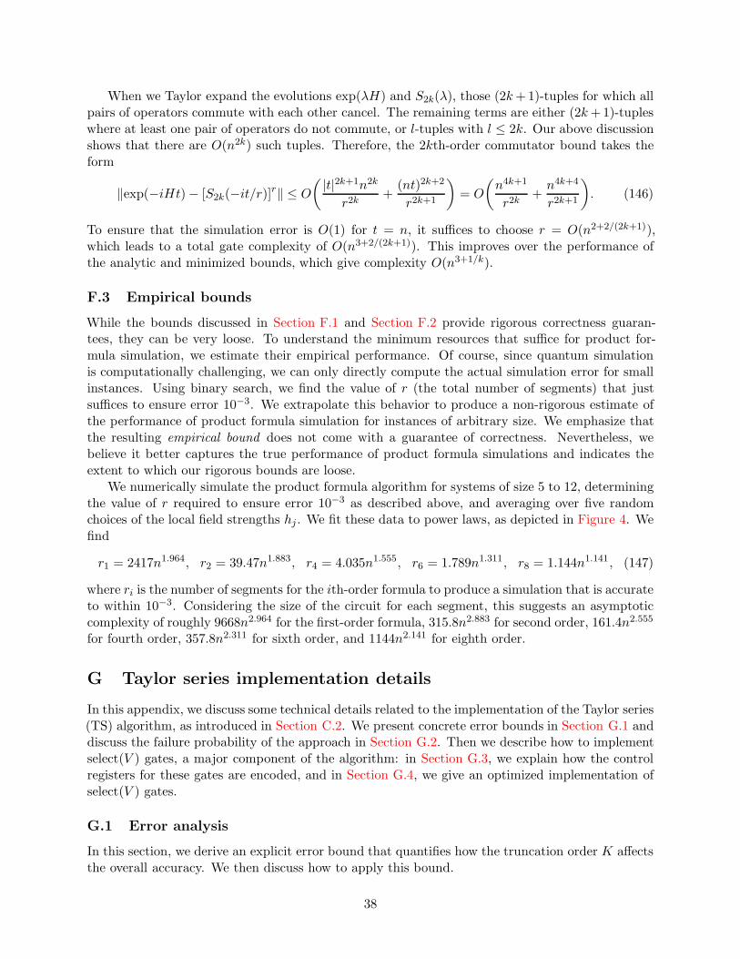
When we Taylor expand the evolutions exp(λH) and S2k(λ), those (2k+1)-tuples for which allpairs of operators commute with each other cancel. The remaining terms are either (2k+1)-tupleswhere at least one pair of operators do not commute, or l-tuples with l ≤ 2k. Our above discussionshows that there are O(n2k) such tuples. Therefore, the 2kth-order commutator bound takes theform

‖exp(−iHt)− [S2k(−it/r)]r‖ ≤ O

( |t|2k+1n2k

r2k+

(nt)2k+2

r2k+1

)

= O

(

n4k+1

r2k+n4k+4

r2k+1

)

. (146)

To ensure that the simulation error is O(1) for t = n, it suffices to choose r = O(n2+2/(2k+1)),which leads to a total gate complexity of O(n3+2/(2k+1)). This improves over the performance ofthe analytic and minimized bounds, which give complexity O(n3+1/k).

F.3 Empirical bounds

While the bounds discussed in Section F.1 and Section F.2 provide rigorous correctness guaran-tees, they can be very loose. To understand the minimum resources that suffice for product for-mula simulation, we estimate their empirical performance. Of course, since quantum simulationis computationally challenging, we can only directly compute the actual simulation error for smallinstances. Using binary search, we find the value of r (the total number of segments) that justsuffices to ensure error 10−3. We extrapolate this behavior to produce a non-rigorous estimate ofthe performance of product formula simulation for instances of arbitrary size. We emphasize thatthe resulting empirical bound does not come with a guarantee of correctness. Nevertheless, webelieve it better captures the true performance of product formula simulations and indicates theextent to which our rigorous bounds are loose.

We numerically simulate the product formula algorithm for systems of size 5 to 12, determiningthe value of r required to ensure error 10−3 as described above, and averaging over five randomchoices of the local field strengths hj . We fit these data to power laws, as depicted in Figure 4. Wefind

r1 = 2417n1.964, r2 = 39.47n1.883, r4 = 4.035n1.555, r6 = 1.789n1.311, r8 = 1.144n1.141, (147)

where ri is the number of segments for the ith-order formula to produce a simulation that is accurateto within 10−3. Considering the size of the circuit for each segment, this suggests an asymptoticcomplexity of roughly 9668n2.964 for the first-order formula, 315.8n2.883 for second order, 161.4n2.555

for fourth order, 357.8n2.311 for sixth order, and 1144n2.141 for eighth order.

G Taylor series implementation details

In this appendix, we discuss some technical details related to the implementation of the Taylor series(TS) algorithm, as introduced in Section C.2. We present concrete error bounds in Section G.1 anddiscuss the failure probability of the approach in Section G.2. Then we describe how to implementselect(V ) gates, a major component of the algorithm: in Section G.3, we explain how the controlregisters for these gates are encoded, and in Section G.4, we give an optimized implementation ofselect(V ) gates.

G.1 Error analysis

In this section, we derive an explicit error bound that quantifies how the truncation order K affectsthe overall accuracy. We then discuss how to apply this bound.

38

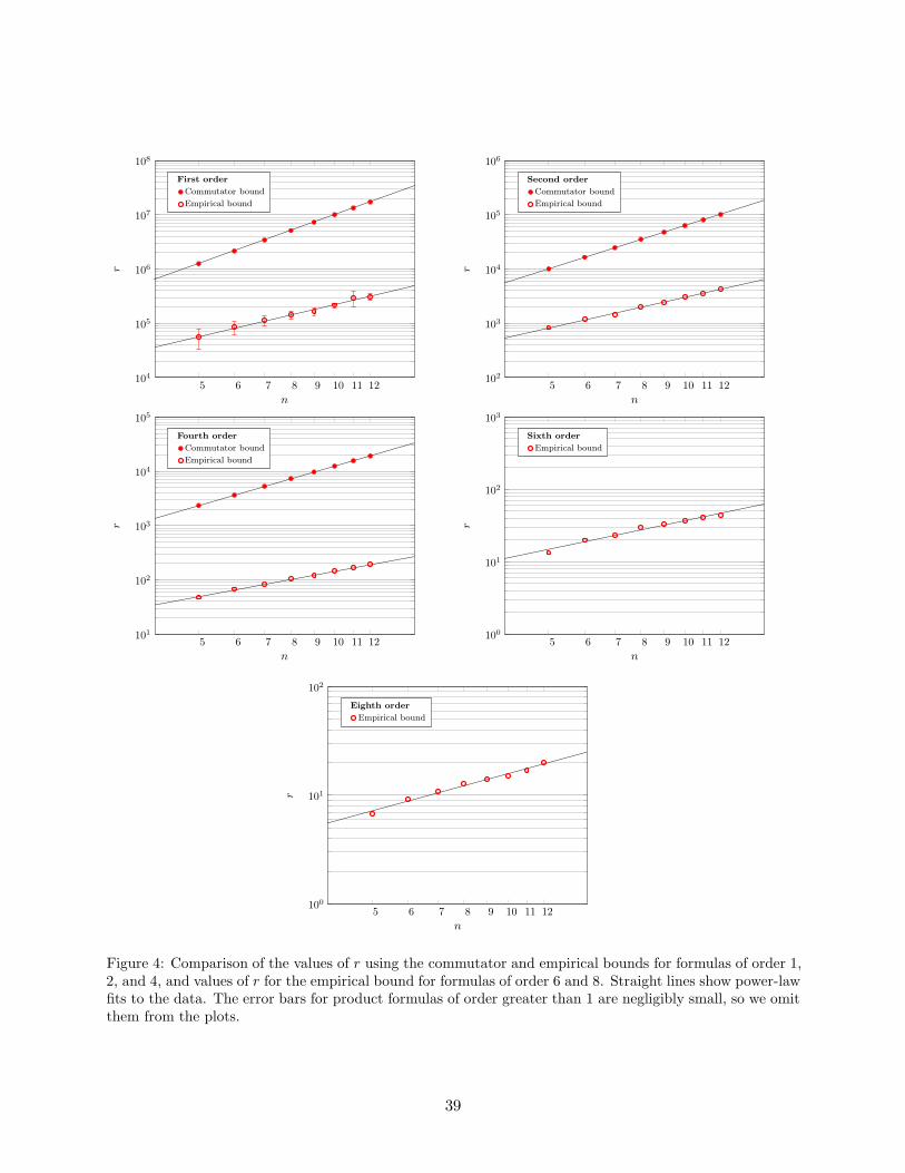
5 6 7 8 9 10 11 12104

105

106

107

108

n

r

First order

Commutator bound

Empirical bound

5 6 7 8 9 10 11 12102

103

104

105

106

n

r

Second order

Commutator bound

Empirical bound

5 6 7 8 9 10 11 12101

102

103

104

105

n

r

Fourth order

Commutator bound

Empirical bound

5 6 7 8 9 10 11 12100

101

102

103

n

r

Sixth order

Empirical bound

5 6 7 8 9 10 11 12100

101

102

n

r

Eighth order

Empirical bound

Figure 4: Comparison of the values of r using the commutator and empirical bounds for formulas of order 1,2, and 4, and values of r for the empirical bound for formulas of order 6 and 8. Straight lines show power-lawfits to the data. The error bars for product formulas of order greater than 1 are negligibly small, so we omitthem from the plots.

39

We begin by bounding the error introduced by truncating the Taylor series.

Lemma G.1. With the definitions of U(t) in (7) and tseg in (18), we have

‖U (t)− exp(−iHt)‖ ≤ 2(ln 2)K+1

(K + 1)!(148)

for any t ≤ tseg.

Proof. We have

‖U(t)− exp(−iHt)‖ =

∥

∥

∥

∥

∥

∞∑

k=K+1

(−iHt)kk!

∥

∥

∥

∥

∥

(149)

≤∞∑

k=K+1

(‖H‖t)kk!

(150)

≤∞∑

k=K+1

((α1 + · · · + αL)t)k

k!(151)

≤∞∑

k=K+1

(ln 2)k

k!(152)

≤ 2(ln 2)K+1

(K + 1)!, (153)

where the final inequality follows from Lemma F.2.

Next we consider the error induced by the isometry V(t) defined in (16). It is straightforwardto verify that

(〈0| ⊗ I)V(t) = 3

sU(t)− 4

s3U(t)U(t)†U(t). (154)

As discussed in Section C.2, we rotate an ancilla qubit to increase the value of s to be preciselys = 2. Then the following bound characterizes the error in the implementation of the Taylor series.

Lemma G.2. Suppose ‖U − U‖ ≤ δ for some unitary operator U . Then∥

∥

∥

∥

3

2U − 1

2U U †U − U

∥

∥

∥

∥

≤ δ2 + 3δ + 4

2δ. (155)

Proof. Since ‖U − U‖ ≤ δ, we have

‖U‖ ≤ ‖U − U‖+ ‖U‖ ≤ 1 + δ (156)

and therefore

‖U U † − I‖ ≤ ‖(U − U)U †‖+ ‖U(U † − U †)‖ ≤ δ(2 + δ). (157)

Thus, by the triangle inequality, we have∥

∥

∥

∥

3

2U − 1

2U U †U − U

∥

∥

∥

∥

≤ ‖U − U‖+ 1

2‖U − U U †U‖ (158)

≤ δ +δ(2 + δ)(1 + δ)

2(159)

=δ2 + 3δ + 4

2δ (160)

as claimed.

40

We use the following basic property of contractions (operators of norm at most 1), which iseasily proved using the triangle inequality.

Lemma G.3. Suppose Ui : H → H and Vi : H → H are contractions for all i ∈ {1, . . . , r}. If‖Ui − Vi‖ ≤ η for all i, then

‖Ur · · ·U2U1 − Vr · · ·V2V1‖ ≤ rη. (161)

We also use the following lemma, which bounds the error introduced by normalization.

Lemma G.4. Suppose ‖|φ〉‖ = 1, ‖|ψ〉‖ ≤ 1, and ‖|ψ〉 − |φ〉‖ ≤ ξ < 1. Then

∥

∥

∥

∥

|ψ〉‖|ψ〉‖ − |φ〉

∥

∥

∥

∥

≤√

1 + ξ −√

1− ξ. (162)

Proof. Decompose |ψ〉 as|ψ〉 = α|φ〉+ β|φ⊥〉 (163)

for some normalized state |φ⊥〉 orthogonal to |φ〉. Clearly |α|2 + |β|2 ≤ 1 since ‖|ψ〉‖ ≤ 1. Further-more, the assumption ‖|ψ〉 − |φ〉‖ ≤ ξ implies

|α− 1|2 + |β|2 ≤ ξ2, (164)

so|α|2 + |β|2 ≤ ξ2 + 2Re(α)− 1 (165)

with 1− ξ ≤ Re(α) ≤ 1 + ξ.Then we have

∥

∥

∥

∥

|ψ〉‖|ψ〉‖ − |φ〉

∥

∥

∥

∥

=

√

2− 2Re(α)√

|α|2 + |β|2(166)

≤√

2− 2Re(α)√

ξ2 + 2Re(α)− 1(167)

≤√

2− 2(1− ξ2)√

ξ2 + 2(1 − ξ2)− 1(168)

=√

1 + ξ −√

1− ξ. (169)

Here the first inequality uses (165) and the fact that Re(α) ≥ 1− ξ ≥ 0, and the second inequalityfollows since the function x/

√

2x− 1 + ξ2 achieves its minimum at x = 1 − ξ2 within the interval1− ξ ≤ x ≤ 1 + ξ.

With all the above lemmas in hand, we are ready to prove an explicit error bound for the TSalgorithm.

Theorem G.5. The TS algorithm achieves error at most√1 + ξ−√

1− ξ with success probabilityat least (1− ξ)2, where

ξ = rδ2 + 3δ + 4

2δ with δ = 2

(ln 2)K+1

(K + 1)!. (170)

41

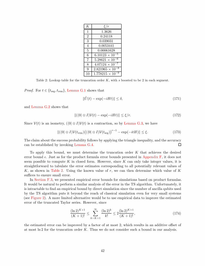
K ξ/r

1 1.3626

2 0.24118

3 0.039031

4 0.0053441

5 0.00061628

6 6.10123 × 10−5

7 5.28621 × 10−6

8 4.07124 × 10−7

9 2.821965 × 10−8

10 1.778215 × 10−9

Table 2: Lookup table for the truncation order K, with s boosted to be 2 in each segment.

Proof. For t ∈ {tseg, trem}, Lemma G.1 shows that

‖U(t)− exp(−iHt)‖ ≤ δ, (171)

and Lemma G.2 shows that

‖(〈0| ⊗ I)V(t) − exp(−iHt)‖ ≤ ξ/r. (172)

Since V(t) is an isometry, (〈0| ⊗ I)V(t) is a contraction, so by Lemma G.3, we have

‖(〈0| ⊗ I)V(trem)(

(〈0| ⊗ I)V(tseg))r−1 − exp(−itH)‖ ≤ ξ. (173)

The claim about the success probability follows by applying the triangle inequality, and the accuracycan be established by invoking Lemma G.4.

To apply this bound, we must determine the truncation order K that achieves the desirederror bound ǫ. Just as for the product formula error bounds presented in Appendix F, it does notseem possible to compute K in closed form. However, since K can only take integer values, it isstraightforward to tabulate the error estimates corresponding to all potentially relevant values ofK, as shown in Table 2. Using the known value of r, we can then determine which value of Ksuffices to ensure small error.

In Section F.3, we presented empirical error bounds for simulations based on product formulas.It would be natural to perform a similar analysis of the error in the TS algorithm. Unfortunately, itis intractable to find an empirical bound by direct simulation since the number of ancilla qubits usedby the TS algorithm puts it beyond the reach of classical simulation even for very small systems(see Figure 2). A more limited alternative would be to use empirical data to improve the estimatederror of the truncated Taylor series. However, since

(ln 2)K+1

(K + 1)!≤

∞∑

k=K+1

(ln 2)k

k!≤ 2

(ln 2)K+1

(K + 1)!, (174)

the estimated error can be improved by a factor of at most 2, which results in an additive offset ofat most ln 2 for the truncation order K. Thus we do not consider such a bound in our analysis.

42

G.2 Failure probability

Note that unlike the PF approach, the TS algorithm does not always succeed. When a measurementof the ancilla register indicates a failure, we must restart the simulation. To make a fair comparisonbetween the PF and TS algorithms, we should take the success probability into account.

Fortunately, it turns out that the resulting overhead is almost negligible. With ǫ = 10−3,Theorem G.5 gives

ξ ≤√

ǫ2 − ǫ4

4< 0.001, (175)

so the success probability of the algorithm is at least

(1− ξ)2 ≥ 0.998. (176)

The expected number of times we must repeat the algorithm before succeeding is approximately1/0.998 ≈ 1.002. Since this factor is very close to 1, we simply neglect it, and we find it reasonableto directly compare gate counts for the PF algorithm (which has no probability of failure) and theTS approach.

G.3 Encoding of the control register

A crucial step in the implementation of the TS algorithm (and in the QSP algorithm) is to synthesizethe select(V ) gates. The cost of this implementation depends strongly on the chosen representationfor the control register.

Recall from (14) that the select(V ) operation has the form

select(V ) :=Γ−1∑

j=0

|j〉〈j| ⊗ Vj. (177)

For the TS algorithm, the operators Vj are defined via (10). Here the index j labels a valuek ∈ {0, 1, . . . ,K} and indices ℓ1, . . . , ℓk ∈ {1, . . . , L}. Perhaps the most straightforward approachis to represent the entire control register with a binary encoding using log2(K +1) +K log2 L bits.However, as pointed out in [14], we can significantly reduce the gate complexity by choosing adifferent encoding of the control register.

Specifically, we use a unary encoding to label k and a binary encoding for each ℓ1, . . . , ℓk. Withsuch an encoding, the instance of select(V ) in the TS algorithm can be represented as the map

|1k0K−k〉|ℓ1, . . . , ℓK〉|ψ〉 7→ |1k0K−k〉|ℓ1, . . . , ℓK〉(−i)kHℓ1 · · ·Hℓk |ψ〉. (178)

We implement this transformation as follows. Conditioned on the jth qubit of the unary encodingof k being 1, and the jth coordinate of ℓ1, . . . , ℓK being the binary encoding of ℓj, we apply(−i)Hℓj . Compared to an entirely binary encoding, this approach only requires an additional⌈K+1− log2(K+1)⌉ qubits, which is a modest increase since K is typically small (see Table 2). Inreturn, instead of selecting on a large register of Θ(K logL) bits, we can perform K+1 independentselections on registers of log2 L bits, each controlled by a single qubit.

G.4 Implementation of select(V )

In this section, we present a circuit for the select(V ) operation∑Γ

γ=1|γ〉〈γ| ⊗ Vγ . We assume thatthe control register γ ∈ {1, . . . ,Γ} is stored in binary using w := ⌈log2 Γ⌉ bits. As discussed in

43

Section G.3, this procedure is a basic subroutine in our implementation of the select(V ) operationappearing in the TS algorithm, using a mixed unary/binary encoding. We also use this select(V )construction in our implementation of the QSP algorithm.

Our goal is to apply a unitary operation Vγ conditioned on the control register being in the state|γ〉. To do this, we cycle the value of a designated ancilla qubit through Γ Boolean products of wliterals, where in each of the products, each of the variables x1, . . . , xw appears exactly once (eithernegated or not). We apply Vγ conditioned on the ancilla qubit at the γth step of this construction.To simplify the presentation, we describe how to cycle through all 2w Boolean products. Thisprocedure can be terminated after producing only Γ Boolean products to avoid unnecessary cost.

A straightforward way of obtaining the Boolean products is to implement them via multiply-controlled Toffoli gates with appropriate control negations. Implementations of the multiply-controlled Toffoli gates have been well-studied. In particular, using the approach of [55], andassuming that the negative controls introduce no additional cost,3 we can cycle through all Booleanproducts using the following resources:

4w2w − 6 · 2w Hadamard gates8w2w − 9 · 2w T/T † gates6w2w − 6 · 2w cnot gates

⌈w−22 ⌉ ancilla qubits, initialized in and returned to the state |0〉.

We now present an optimized circuit to cycle through these Boolean products. In particular,we do this using a reversible circuit consisting of not, cnot, and Toffoli gates (we call a circuitover this gate set an NCT circuit). Of the three basic gates used by the NCT circuits, the Toffoligate is the most expensive—its best known implementation uses 6 cnot gates, 2 Hadamard gates,and 7 T/T † gates [2]—so we first focus on optimizing the Toffoli gate count. We use Toffoli gateswith controls of arbitrary polarities. All such Toffoli gates can be implemented by a Clifford+Tcircuit using the same resources [2].

To cycle though 2w Boolean products, clearly we must use at least 2w gates (note that we do notallow gates with multiple targets). Indeed, most of these must be Toffoli gates, the most expensivegates in an NCT circuit.

Lemma G.6 ([56, Lemma 4]). An NCT circuit for select(V ) control generation requires at least2w − w − 1 Toffoli gates.

Considering the cost of a single Toffoli gate, a Clifford+T circuit with 2w Toffoli gates couldcontain as many as 6 · 2w cnot gates and 7 · 2w T/T † gates. We next construct a quantumcircuit that cycles through all 2w Boolean products, and show that after several optimizations, thegate counts are close to the above optimistic figure, and significantly better than those obtainedusing multiply-controlled Toffoli gates. We begin by describing an efficient NCT circuit that cyclesthrough 2w Boolean products.

Lemma G.7. The select(V ) control generation can be implemented by an NCT circuit using atmost 2 not gates, 1.5 · 2w − 2 cnot gates, and 1.5 · 2w − 4 Toffoli gates, with w − 1 ancilla qubitsinitialized in and returned to the state |0〉.

Proof. Consider a depth-w complete binary tree, where vertices are labeled by the Boolean productsof the w variables x1, . . . , xw. A vertex at depth d is labeled by a product of the first d variables,

3While a construction with this property was not explicitly developed in [55], it appears that any multiply-controlled Toffoli gate with arbitrary positive and negative controls can be implemented with the same number ofgates as the multiply-controlled Toffoli gate of the same size with only positive controls.

44

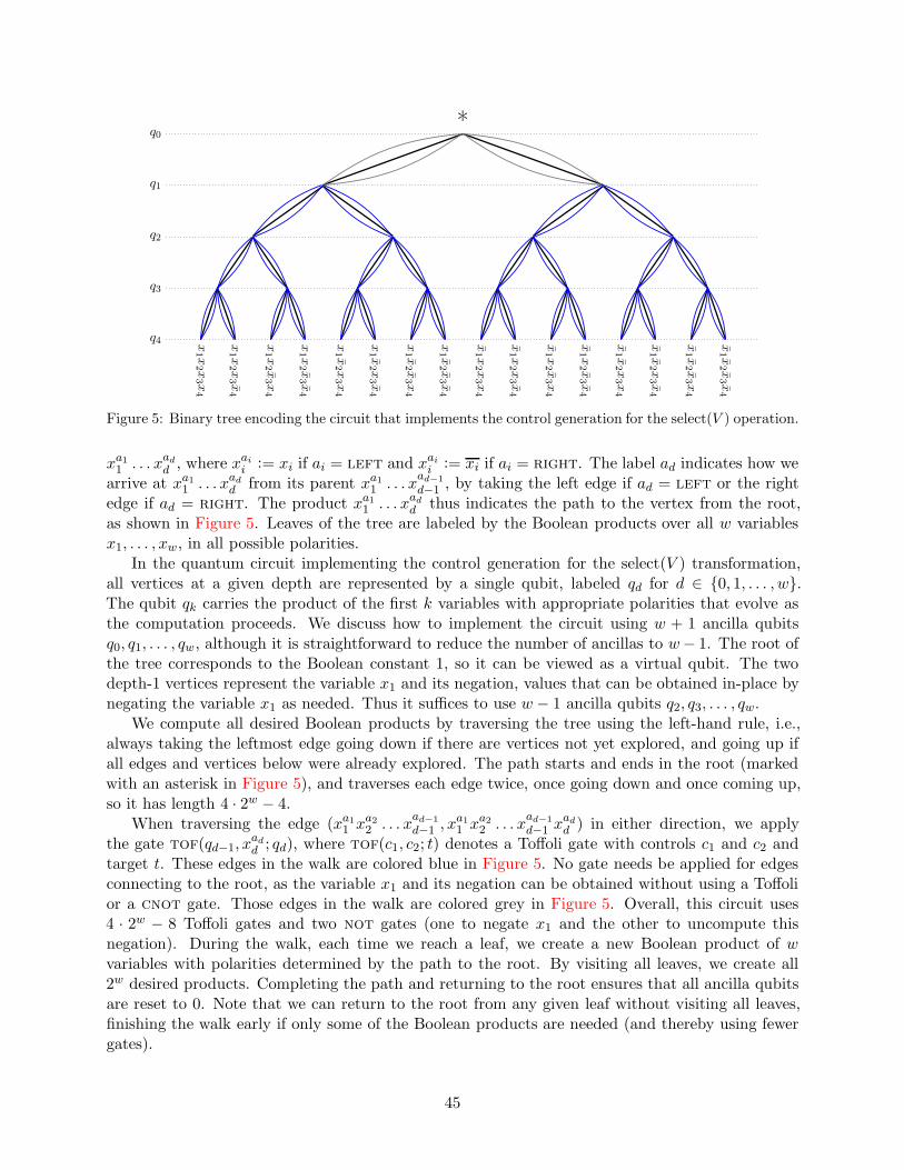
q0

q1

q2

q3

q4

*

x1 x

2 x3 x

4

x1 x

2 x3 x

4

x1 x

2 x3 x

4

x1 x

2 x3 x

4

x1 x

2 x3 x

4

x1 x

2 x3 x

4

x1 x

2 x3 x

4

x1 x

2 x3 x

4

x1 x

2 x3 x

4

x1 x

2 x3 x

4

x1 x

2 x3 x

4

x1 x

2 x3 x

4

x1 x

2 x3 x

4

x1 x

2 x3 x

4

x1 x

2 x3 x

4

x1 x

2 x3 x

4

Figure 5: Binary tree encoding the circuit that implements the control generation for the select(V ) operation.

xa11 . . . xadd , where xaii := xi if ai = left and xaii := xi if ai = right. The label ad indicates how wearrive at xa11 . . . xadd from its parent xa11 . . . x

ad−1

d−1 , by taking the left edge if ad = left or the rightedge if ad = right. The product xa11 . . . xadd thus indicates the path to the vertex from the root,as shown in Figure 5. Leaves of the tree are labeled by the Boolean products over all w variablesx1, . . . , xw, in all possible polarities.

In the quantum circuit implementing the control generation for the select(V ) transformation,all vertices at a given depth are represented by a single qubit, labeled qd for d ∈ {0, 1, . . . , w}.The qubit qk carries the product of the first k variables with appropriate polarities that evolve asthe computation proceeds. We discuss how to implement the circuit using w + 1 ancilla qubitsq0, q1, . . . , qw, although it is straightforward to reduce the number of ancillas to w− 1. The root ofthe tree corresponds to the Boolean constant 1, so it can be viewed as a virtual qubit. The twodepth-1 vertices represent the variable x1 and its negation, values that can be obtained in-place bynegating the variable x1 as needed. Thus it suffices to use w − 1 ancilla qubits q2, q3, . . . , qw.

We compute all desired Boolean products by traversing the tree using the left-hand rule, i.e.,always taking the leftmost edge going down if there are vertices not yet explored, and going up ifall edges and vertices below were already explored. The path starts and ends in the root (markedwith an asterisk in Figure 5), and traverses each edge twice, once going down and once coming up,so it has length 4 · 2w − 4.

When traversing the edge (xa11 xa22 . . . x

ad−1

d−1 , xa11 x

a22 . . . x

ad−1

d−1 xadd ) in either direction, we apply

the gate tof(qd−1, xadd ; qd), where tof(c1, c2; t) denotes a Toffoli gate with controls c1 and c2 and

target t. These edges in the walk are colored blue in Figure 5. No gate needs be applied for edgesconnecting to the root, as the variable x1 and its negation can be obtained without using a Toffolior a cnot gate. Those edges in the walk are colored grey in Figure 5. Overall, this circuit uses4 · 2w − 8 Toffoli gates and two not gates (one to negate x1 and the other to uncompute thisnegation). During the walk, each time we reach a leaf, we create a new Boolean product of wvariables with polarities determined by the path to the root. By visiting all leaves, we create all2w desired products. Completing the path and returning to the root ensures that all ancilla qubitsare reset to 0. Note that we can return to the root from any given leaf without visiting all leaves,finishing the walk early if only some of the Boolean products are needed (and thereby using fewergates).

45

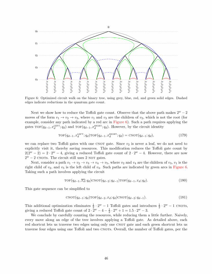
q0

q1

q2

q3

q4

*

x1 x

2 x3 x

4

x1 x

2 x3 x

4

x1 x

2 x3 x

4

x1 x

2 x3 x

4

x1 x

2 x3 x

4

x1 x

2 x3 x

4

x1 x

2 x3 x

4

x1 x

2 x3 x

4

x1 x

2 x3 x

4

x1 x

2 x3 x

4

x1 x

2 x3 x

4

x1 x

2 x3 x

4

x1 x

2 x3 x

4

x1 x

2 x3 x

4

x1 x

2 x3 x

4

x1 x

2 x3 x

4

Figure 6: Optimized circuit walk on the binary tree, using grey, blue, red, and green solid edges. Dashededges indicate reductions in the quantum gate count.

Next we show how to reduce the Toffoli gate count. Observe that the above path makes 2w − 2moves of the form v1 → v2 → v3, where v1 and v3 are the children of v2, which is not the root (forexample, consider any path indicated by a red arc in Figure 6). Such a path requires applying thegates tof(qd−1, x

left

d ; qd) and tof(qd−1, xright

d ; qd). However, by the circuit identity

tof(qd−1, xleft

d ; qd)tof(qd−1, xright

d ; qd) = cnot(qd−1; qd), (179)

we can replace two Toffoli gates with one cnot gate. Since v2 is never a leaf, we do not need toexplicitly visit it, thereby saving resources. This modification reduces the Toffoli gate count by2(2w − 2) = 2 · 2w − 4, giving a reduced Toffoli gate count of 2 · 2w − 4. However, there are now2w − 2 cnots. The circuit still uses 2 not gates.

Next, consider a path v1 → v2 → v3 → v4 → v5, where v2 and v4 are the children of v3, v1 is theright child of v2, and v5 is the left child of v4. Such paths are indicated by green arcs in Figure 6.Taking such a path involves applying the circuit

tof(qd−1, xd; qd)cnot(qd−2; qd−1)tof(qd−1, xd; qd). (180)

This gate sequence can be simplified to

cnot(qd−1; qd)tof(qd−2, xd; qd)cnot(qd−2; qd−1). (181)

This additional optimization eliminates 12 · 2w − 1 Toffoli gates and introduces 1

2 · 2w − 1 cnots,giving a reduced Toffoli gate count of 2 · 2w − 4− 1

2 · 2w + 1 = 1.5 · 2w − 3.We conclude by carefully counting the resources, while reducing them a little further. Naively,

every move along an edge of the tree involves applying a Toffoli gate. As detailed above, eachred shortcut lets us traverse two edges using only one cnot gate and each green shortcut lets ustraverse four edges using one Toffoli and two cnots. Overall, the number of Toffoli gates, per the

46

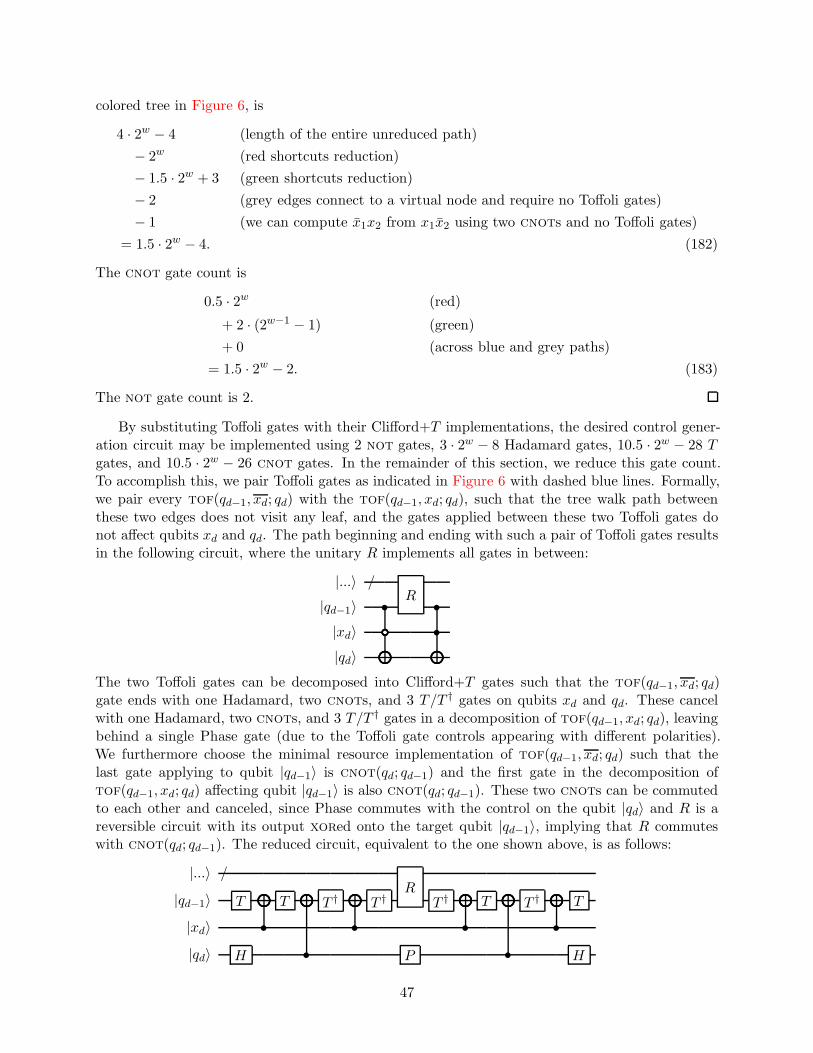
colored tree in Figure 6, is

4 · 2w − 4 (length of the entire unreduced path)

− 2w (red shortcuts reduction)

− 1.5 · 2w + 3 (green shortcuts reduction)

− 2 (grey edges connect to a virtual node and require no Toffoli gates)

− 1 (we can compute x1x2 from x1x2 using two cnots and no Toffoli gates)

= 1.5 · 2w − 4. (182)

The cnot gate count is

0.5 · 2w (red)

+ 2 · (2w−1 − 1) (green)

+ 0 (across blue and grey paths)

= 1.5 · 2w − 2. (183)

The not gate count is 2.

By substituting Toffoli gates with their Clifford+T implementations, the desired control gener-ation circuit may be implemented using 2 not gates, 3 · 2w − 8 Hadamard gates, 10.5 · 2w − 28 Tgates, and 10.5 · 2w − 26 cnot gates. In the remainder of this section, we reduce this gate count.To accomplish this, we pair Toffoli gates as indicated in Figure 6 with dashed blue lines. Formally,we pair every tof(qd−1, xd; qd) with the tof(qd−1, xd; qd), such that the tree walk path betweenthese two edges does not visit any leaf, and the gates applied between these two Toffoli gates donot affect qubits xd and qd. The path beginning and ending with such a pair of Toffoli gates resultsin the following circuit, where the unitary R implements all gates in between:

|...〉 /R

|qd−1〉 • •|xd〉 •|qd〉

The two Toffoli gates can be decomposed into Clifford+T gates such that the tof(qd−1, xd; qd)gate ends with one Hadamard, two cnots, and 3 T/T † gates on qubits xd and qd. These cancelwith one Hadamard, two cnots, and 3 T/T † gates in a decomposition of tof(qd−1, xd; qd), leavingbehind a single Phase gate (due to the Toffoli gate controls appearing with different polarities).We furthermore choose the minimal resource implementation of tof(qd−1, xd; qd) such that thelast gate applying to qubit |qd−1〉 is cnot(qd; qd−1) and the first gate in the decomposition oftof(qd−1, xd; qd) affecting qubit |qd−1〉 is also cnot(qd; qd−1). These two cnots can be commutedto each other and canceled, since Phase commutes with the control on the qubit |qd〉 and R is areversible circuit with its output xored onto the target qubit |qd−1〉, implying that R commuteswith cnot(qd; qd−1). The reduced circuit, equivalent to the one shown above, is as follows:

|...〉 /R

|qd−1〉 T T T † T † T † T T † T

|xd〉 • • • •|qd〉 H • P • H

47

The equivalence of the circuits before and after optimization can be verified by direct computation.The control generation circuit contains 1

2 · 2w − w such Toffoli pairs, each reducing the gatecount by 2 Hadamards, 6 T/T † gates, and 6 cnots while introducing a single Phase gate. Overall,the optimized select(V ) control generation circuit thus uses the following resources:

2 not gates2 · 2w + 2w − 8 Hadamard gates

0.5 · 2w − w Phase gates7.5 · 2w + 6w − 28 T/T † gates7.5 · 2w + 6w − 26 cnot gates

w − 1 ancilla qubits, initialized in and returned to the state |0〉.Note that the resulting T/T †-count is only about 7% higher than the expected T/T †-count in

a circuit with 2w −w− 1 Toffoli gates (which is the number of Toffoli gates required to generate 2w

Boolean products by a reversible NCT circuit, according to Lemma G.6). The overall elementarygate count in our optimized implementation is 17.5 · 2w + o(2w). This compares favorably to thebaseline estimation of 18w2w + o(w2w) elementary gates, improving the gate count by a factor of36w35 at leading order. Recall that in our application to the TS algorithm, we have w = ⌈log2 Γ⌉,where Γ is the number of selected unitaries, as in (177).

H Quantum signal processing implementation details

We now turn our attention to the quantum signal processing (QSP) algorithm of Low and Chuang[51, 52], as introduced in Section C.3. We estimate the success probability of the QSP algorithm inSection H.1 and discuss how this can be taken into account to make a fair comparison with othersimulation algorithms. In Section H.2, we describe optimizations that reduce the gate count ofour implementation. Then, in Section H.3, we discuss the difficulty of computing the phases thatspecify the algorithm and describe a segmented version of the algorithm that mitigates this issue.Finally, in Section H.4, we describe empirical bounds on the error in the truncated Jacobi-Angerexpansion and in the overall algorithm.

H.1 Failure probability

Just like the TS algorithm, the QSP algorithm is probabilistic. The success probability is notexplicitly evaluated in references [51, 52]. The error analysis presented in Section C.3 guaranteesthat the post-selected operator (〈+|〈G| ⊗ I)V (|+〉|G〉 ⊗ I) is close to the ideal evolution e−iHt inthe sense that

∥

∥

(

〈+|〈G| ⊗ I)

V(

|+〉|G〉 ⊗ I)

− e−iHt∥

∥ ≤ ǫ. (184)

Therefore, for any given input state |ψ〉, the postselection succeeds with probability at least∥

∥

(

〈+|〈G| ⊗ I)

V(

|+〉|G〉 ⊗ |ψ〉)∥

∥

2

≥(∥

∥e−iHt|ψ〉∥

∥ −∥

∥

(

〈+|〈G| ⊗ I)

V(

|+〉|G〉 ⊗ |ψ〉)

− e−iHt|ψ〉∥

∥

)2(185)

≥(

1−∥

∥

(

〈+|〈G| ⊗ I)

V(

|+〉|G〉 ⊗ I)

− e−iHt∥

∥

)2(186)

≥ 1− 2ǫ. (187)

With ǫ = 10−3, the success probability of the QSP algorithm is at least 1− 2ǫ = 0.998. Reasoningsimilarly as in Section G.2, we find that the expected number of times we must repeat the algorithmbefore succeeding is approximately 1/0.998 ≈ 1.002. This factor is very close to 1, so as for the TSalgorithm, we neglect it when comparing gate counts.

48

H.2 Circuit optimizations

The select(V ) gate is a major component of the QSP algorithm, so we use the optimized implemen-tation of that subroutine described in Section G.4 in our implementation of the QSP algorithm. Inthis section, we present some further circuit optimizations that also reduce the gate count.

As discussed in Section C.3, we use the phased iterate Vφ defined in (31), whereas Low andChuang use the operation V ′

φ defined in (40). It is easy to see that

Vφ = (I ⊗ Zπ/2)V′φ(I ⊗ Z−π/2), (188)

so

V †φ = (I ⊗ Zπ/2)V

′†φ (I ⊗ Z−π/2) (189)

also involves conjugation by I ⊗ Zπ/2. Thus, when the phased iterates are applied in the sequence(35), the inner partial reflection gates cancel. Furthermore, Zϕ simply introduces a relative phasebetween |G〉 and its orthogonal subspace, so its action is trivial if the ancilla register is initializedin and postselected on |G〉. Thus we see that the implementation as defined in Section C.3 has thesame effect as in [51]. Each partial reflection is implemented using O(log n) elementary gates, andthere are O(n2) phased iterates, so our implementation saves O(n2 log n) gates.

We apply a similar simplification to further reduce the gate count. For every phased iterateVφ defined in (31), we must implement a controlled version of the operator −iQ = −i

(

(2|G〉〈G| −I) ⊗ I

)

select(H). In particular, this requires us to perform a controlled-reflection about |G〉. Wecan do this by performing a controlled-U † that unprepares the state |G〉 (where U is a unitaryoperation satisfying U |0〉 = |G〉), a controlled reflection about |0〉, and finally a controlled-U thatprepares the state |G〉. However, observe that we can replace the controlled unitary conjugationby its uncontrolled version without changing the behavior of the circuit. Furthermore, by groupingneighboring pairs of phased iterates in the sequence of Vφ and V †

φ′ operations, we can cancel pairs

of unitary operators U and U † for state preparation and unpreparation.

H.3 Phase computation and segmented algorithm

Recall that to specify the QSP algorithm, we must find phases φ1, . . . , φM that realize the truncatedJacobi-Anger expansion. In principle, these angles can be computed in polynomial time [53]. How-ever, this computation is difficult in practice, so we can only carry it out for very small instances.Specifically, we found the time required to calculate the angles to be prohibitive for values of Mgreater than about 32. For n = 10 qubits with t = n and ǫ = 10−3, the error bound (38) suggeststhat we should take M = 1100. Thus the difficulty of computing the angles prevents us fromsynthesizing nontrivial instances of the algorithm. This difficulty arises because the procedure forcomputing the angles requires us to compute the roots of a high-degree polynomial to high precision.It is a natural open problem to give a more practical method for computing the angles.

Fortunately, to determine the Clifford+Rz gate count in our implementation of the QSP al-gorithm, we do not need to know the angles of the phased iterates. Furthermore, since most Rz

gates require approximately the same number of Hadamard and T gates to realize within a givenprecision, we can get a reasonable estimate of the Clifford+T count by using random angles in placeof the true values. However, we emphasize that this method does not produce a correct quantumsimulation circuit, and should only be used as a benchmark of the resource requirements of theQSP algorithm—which is only useful if the true angles can ultimately be computed.

An alternative is to consider what we call a segmented version of the algorithm. In this approach,we first divide the evolution time into r segments, each of which is sufficiently short that the angles

49

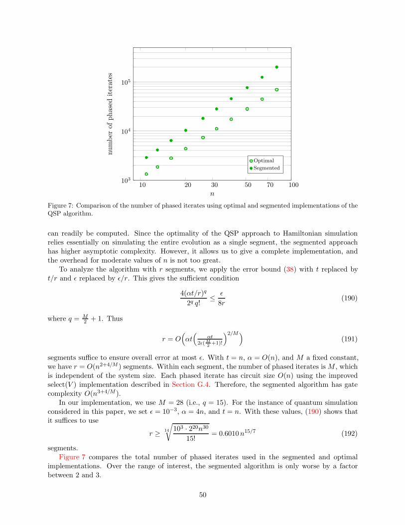
10 20 30 50 70 100103

104

105

n

number

ofphased

iterates

Optimal

Segmented

Figure 7: Comparison of the number of phased iterates using optimal and segmented implementations of theQSP algorithm.

can readily be computed. Since the optimality of the QSP approach to Hamiltonian simulationrelies essentially on simulating the entire evolution as a single segment, the segmented approachhas higher asymptotic complexity. However, it allows us to give a complete implementation, andthe overhead for moderate values of n is not too great.

To analyze the algorithm with r segments, we apply the error bound (38) with t replaced byt/r and ǫ replaced by ǫ/r. This gives the sufficient condition

4(αt/r)q

2q q!≤ ǫ

8r(190)

where q = M2 + 1. Thus

r = O(

αt(

αt2ǫ(M

2+1)!

)2/M)

(191)

segments suffice to ensure overall error at most ǫ. With t = n, α = O(n), and M a fixed constant,we have r = O(n2+4/M ) segments. Within each segment, the number of phased iterates isM , whichis independent of the system size. Each phased iterate has circuit size O(n) using the improvedselect(V ) implementation described in Section G.4. Therefore, the segmented algorithm has gatecomplexity O(n3+4/M ).

In our implementation, we use M = 28 (i.e., q = 15). For the instance of quantum simulationconsidered in this paper, we set ǫ = 10−3, α = 4n, and t = n. With these values, (190) shows thatit suffices to use

r ≥ 14

√

103 · 220n3015!

= 0.6010n15/7 (192)

segments.Figure 7 compares the total number of phased iterates used in the segmented and optimal

implementations. Over the range of interest, the segmented algorithm is only worse by a factorbetween 2 and 3.

50

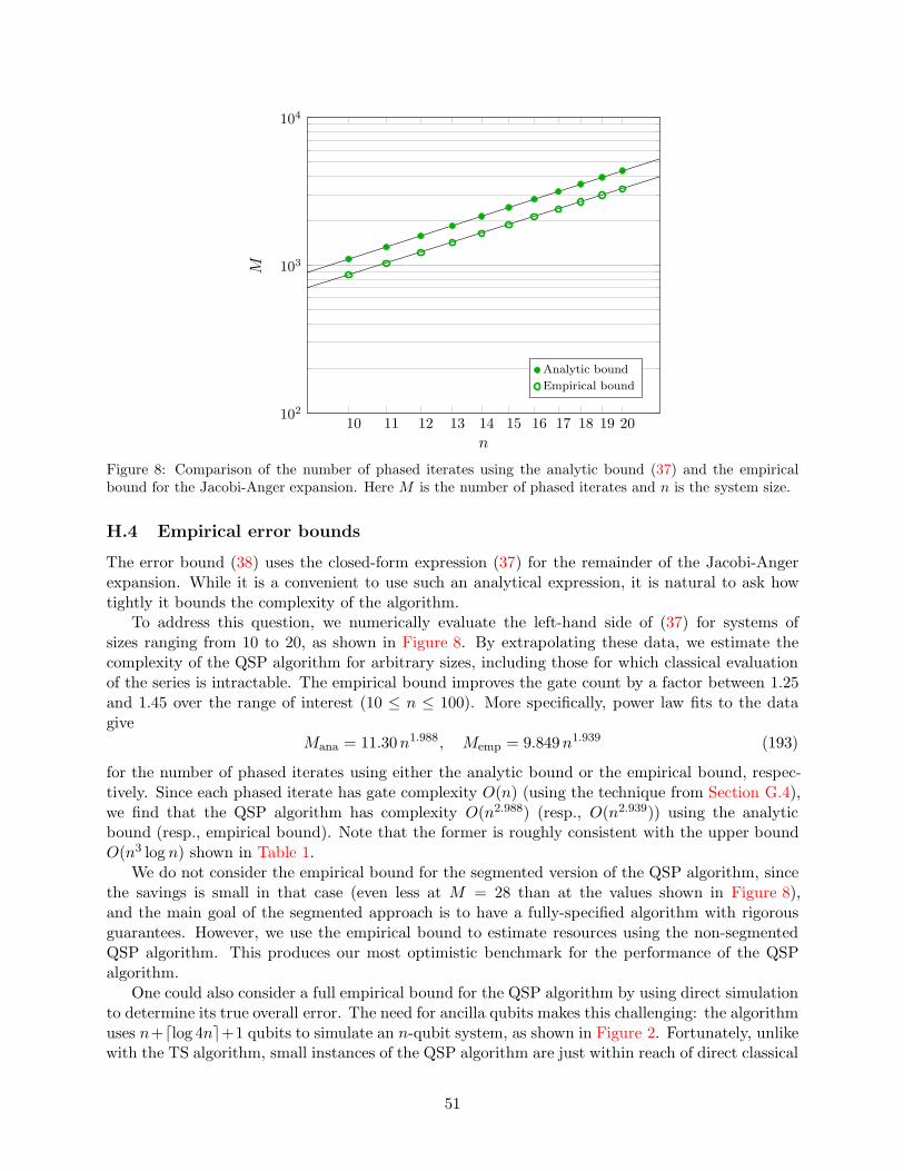
10 11 12 13 14 15 16 17 18 19 20102

103

104

n

M

Analytic bound

Empirical bound

Figure 8: Comparison of the number of phased iterates using the analytic bound (37) and the empiricalbound for the Jacobi-Anger expansion. Here M is the number of phased iterates and n is the system size.

H.4 Empirical error bounds

The error bound (38) uses the closed-form expression (37) for the remainder of the Jacobi-Angerexpansion. While it is a convenient to use such an analytical expression, it is natural to ask howtightly it bounds the complexity of the algorithm.

To address this question, we numerically evaluate the left-hand side of (37) for systems ofsizes ranging from 10 to 20, as shown in Figure 8. By extrapolating these data, we estimate thecomplexity of the QSP algorithm for arbitrary sizes, including those for which classical evaluationof the series is intractable. The empirical bound improves the gate count by a factor between 1.25and 1.45 over the range of interest (10 ≤ n ≤ 100). More specifically, power law fits to the datagive

Mana = 11.30n1.988, Memp = 9.849n1.939 (193)

for the number of phased iterates using either the analytic bound or the empirical bound, respec-tively. Since each phased iterate has gate complexity O(n) (using the technique from Section G.4),we find that the QSP algorithm has complexity O(n2.988) (resp., O(n2.939)) using the analyticbound (resp., empirical bound). Note that the former is roughly consistent with the upper boundO(n3 log n) shown in Table 1.

We do not consider the empirical bound for the segmented version of the QSP algorithm, sincethe savings is small in that case (even less at M = 28 than at the values shown in Figure 8),and the main goal of the segmented approach is to have a fully-specified algorithm with rigorousguarantees. However, we use the empirical bound to estimate resources using the non-segmentedQSP algorithm. This produces our most optimistic benchmark for the performance of the QSPalgorithm.

One could also consider a full empirical bound for the QSP algorithm by using direct simulationto determine its true overall error. The need for ancilla qubits makes this challenging: the algorithmuses n+⌈log 4n⌉+1 qubits to simulate an n-qubit system, as shown in Figure 2. Fortunately, unlikewith the TS algorithm, small instances of the QSP algorithm are just within reach of direct classical

51

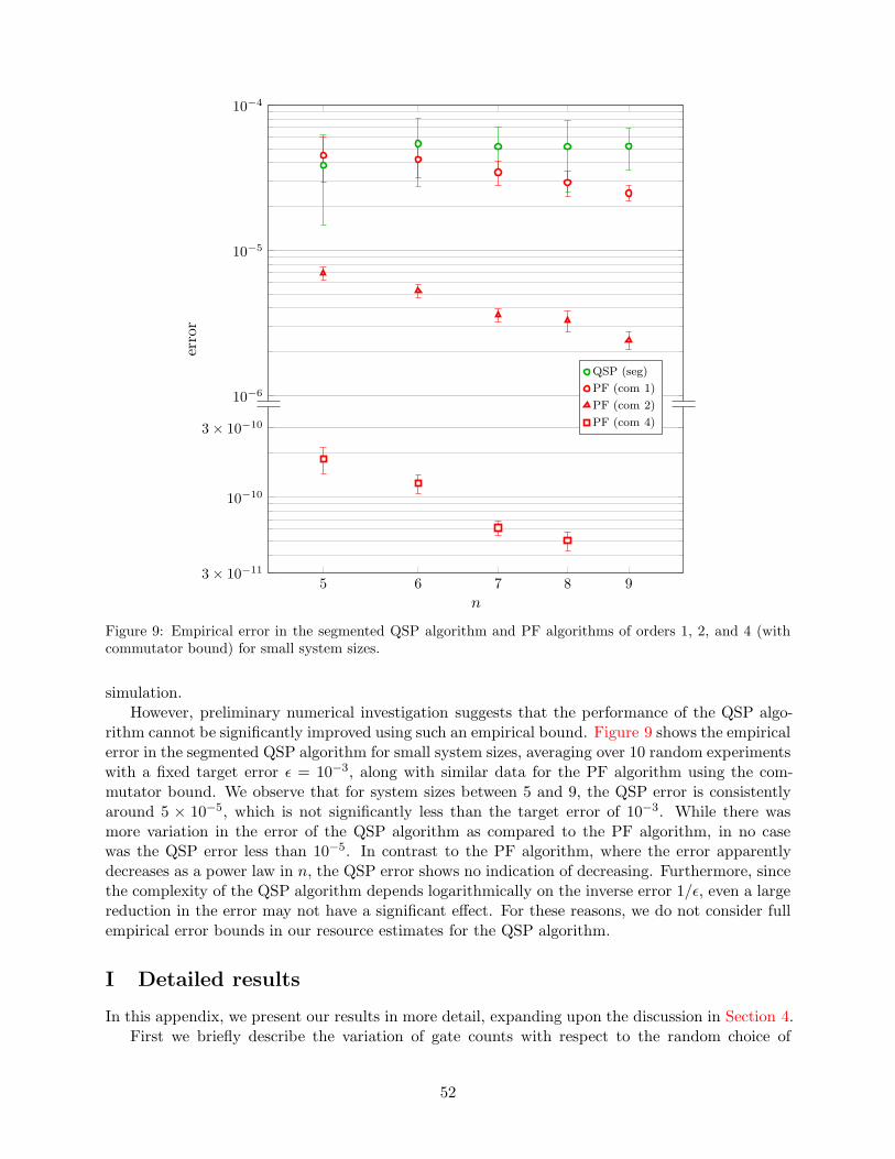
10−6

10−5

10−4

error

5 6 7 8 93× 10−11

10−10

3× 10−10

n

QSP (seg)

PF (com 1)

PF (com 2)

PF (com 4)

Figure 9: Empirical error in the segmented QSP algorithm and PF algorithms of orders 1, 2, and 4 (withcommutator bound) for small system sizes.

simulation.However, preliminary numerical investigation suggests that the performance of the QSP algo-

rithm cannot be significantly improved using such an empirical bound. Figure 9 shows the empiricalerror in the segmented QSP algorithm for small system sizes, averaging over 10 random experimentswith a fixed target error ǫ = 10−3, along with similar data for the PF algorithm using the com-mutator bound. We observe that for system sizes between 5 and 9, the QSP error is consistentlyaround 5 × 10−5, which is not significantly less than the target error of 10−3. While there wasmore variation in the error of the QSP algorithm as compared to the PF algorithm, in no casewas the QSP error less than 10−5. In contrast to the PF algorithm, where the error apparentlydecreases as a power law in n, the QSP error shows no indication of decreasing. Furthermore, sincethe complexity of the QSP algorithm depends logarithmically on the inverse error 1/ǫ, even a largereduction in the error may not have a significant effect. For these reasons, we do not consider fullempirical error bounds in our resource estimates for the QSP algorithm.

I Detailed results

In this appendix, we present our results in more detail, expanding upon the discussion in Section 4.First we briefly describe the variation of gate counts with respect to the random choice of

52

Hamiltonian (namely, the coefficients hj ∈ [−1, 1] in (1)). For each of the system sizes consideredbelow, we generated five random Hamiltonians and determined the gate counts using Quipper. Wereport the average gate count over the five Hamiltonians.

In the Clifford+Rz basis, the gate counts for PF algorithms are actually independent of theparticular choice of coefficients hj : the rotation angles in the circuits differ, but the number ofrotations does not. The number of gates in the Clifford+T basis depends on these angles, but onlyweakly. Across orders and bounds, the T count never varies by more than 1%. The TS algorithmis the most sensitive to the choice of Hamiltonian. For systems of size 13, the Clifford+Rz gatecounts vary by about 10%, and similarly for the T counts. However, the variance reduces as thesystem size increases. For systems of size 100, the variance is about 2% across gate types. The QSPalgorithm (segmented or not) has a mild dependence on the random choice of Hamiltonian. In theClifford+Rz basis, the cnot and Rz counts are independent of the choice of Hamiltonian while theClifford counts vary by less than 1%. Because the rotation angles depend on the Hamiltonian, theT count depends on the choice of Hamiltonian, but again the observed variation is always less than1%.

In the remainder of this section, we present our results in detail. We discuss the PF algorithmfirst, in Section I.1, since this case has the most variations to compare. Then, in Section I.2, wepresent results for the TS and QSP algorithms and discuss the relative performance of all threeapproaches. In Section I.3, we explain how the circuit counts are improved using our automatedcircuit optimizer.

I.1 Product formulas

The performance of quantum simulation algorithms using product formulas depends strongly onthe order of the formula and the method used to bound its error. We now compare the effect ofthese choices.

Figure 10 compares the total gate counts of simulation algorithms using product formulas ofvarious orders with each of our four error bounds. Using rigorous bounds, for system sizes between13 and 500, the fourth-order algorithm outperforms other orders except for very small system sizes.The second-order algorithm is preferred for the largest range of system sizes with the minimizedbound, but even in that case, it only outperforms the fourth-order algorithm for n ≤ 28. Similarconsiderations hold for Clifford+T circuits and when we only count gates of a particular type.Overall, it is clear that the fourth-order algorithm using the commutator bound is preferred for ourapplication if one requires a provable guarantee on the error. If a heuristic method is acceptable, theempirical bound offers a dramatic reduction in complexity. In that case, the sixth-order algorithmbegins to outperform the fourth-order algorithm at around 30 qubits, although the difference issmall for the range of sizes we focus on (at most 100 qubits).

Of the cases we considered, the first-order algorithm has the worst performance, using from102 to over 104 times more gates than the fourth- or sixth-order algorithm. The experimentaldemonstrations of digital quantum simulation that we are aware of [6, 19, 48] have primarily usedthe first-order formula, with some limited applications of the second-order formula [19, 48]. Ourwork suggests that higher-order formulas may be practically relevant for surprisingly small instances,and we hope our results motivate practitioners to take advantage of this.

We did not evaluate the commutator bound for orders higher than 4. This is because the boundis difficult to compute in practice, as discussed in Section F.2. Since the fourth-order algorithmperforms significantly better than the sixth-order one for both the analytic and minimized bounds,we also expect the fourth-order algorithm to outperform the sixth-order algorithm even if we usedan analogous sixth-order commutator bound.

53

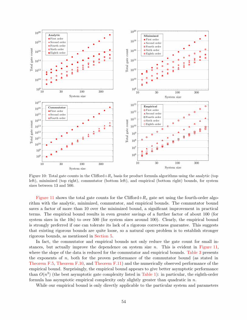
10 100108

1010

1012

1014

1016

1018

1020

30 300

System size

Total

gate

count

Analytic

First order

Second order

Fourth order

Sixth order

Eighth order

10 100108

1010

1012

1014

1016

1018

1020

30 300

System size

Total

gate

count

Minimized

First order

Second order

Fourth order

Sixth order

Eighth order

10 100

108

109

1010

1011

1012

1013

1014

1015

1016

1017

30 300

System size

Total

gate

count

Commutator

First order

Second order

Fourth order

10 100

106

107

108

109

1010

1011

1012

1013

30 300

System size

Total

gate

count

Empirical

First order

Second order

Fourth order

Sixth order

Eighth order

Figure 10: Total gate counts in the Clifford+Rz basis for product formula algorithms using the analytic (topleft), minimized (top right), commutator (bottom left), and empirical (bottom right) bounds, for systemsizes between 13 and 500.

Figure 11 shows the total gate counts for the Clifford+Rz gate set using the fourth-order algo-rithm with the analytic, minimized, commutator, and empirical bounds. The commutator boundsaves a factor of more than 10 over the minimized bound, a significant improvement in practicalterms. The empirical bound results in even greater savings of a further factor of about 100 (forsystem sizes in the 10s) to over 500 (for system sizes around 100). Clearly, the empirical boundis strongly preferred if one can tolerate its lack of a rigorous correctness guarantee. This suggeststhat existing rigorous bounds are quite loose, so a natural open problem is to establish strongerrigorous bounds, as mentioned in Section 5.

In fact, the commutator and empirical bounds not only reduce the gate count for small in-stances, but actually improve the dependence on system size n. This is evident in Figure 11,where the slope of the data is reduced for the commutator and empirical bounds. Table 3 presentsthe exponents of n, both for the proven performance of the commutator bound (as stated inTheorem F.5, Theorem F.10, and Theorem F.11) and the numerically observed performance of theempirical bound. Surprisingly, the empirical bound appears to give better asymptotic performancethan O(n3) (the best asymptotic gate complexity listed in Table 1): in particular, the eighth-orderformula has asymptotic empirical complexity only slightly greater than quadratic in n.

While our empirical bound is only directly applicable to the particular system and parameters

54

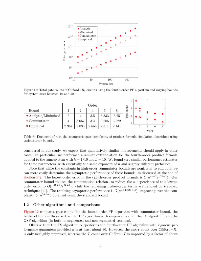
10 100105

107

109

1011

1013

1015

30 300

System size

Total

gate

count

AnalyticMinimizedCommutatorEmpirical

Figure 11: Total gate counts of Clifford+Rz circuits using the fourth-order PF algorithm and varying boundsfor system sizes between 10 and 500.

Order

Bound 1 2 4 6 8

Analytic/Minimized 5 4 3.5 3.333 3.25

Commutator 4 3.667 3.4 3.286 3.222

Empirical 2.964 2.883 2.555 2.311 2.141 2 4 6 82

3

4

5

1

Order

Exponen

t

Table 3: Exponent of n in the asymptotic gate complexity of product formula simulation algorithms usingvarious error bounds.

considered in our study, we expect that qualitatively similar improvements should apply in othercases. In particular, we performed a similar extrapolation for the fourth-order product formulaapplied to the same system with h = 1/10 and h = 10. We found very similar performance estimatesfor these parameters, with essentially the same exponent of n and slightly different prefactors.

Note that while the constants in high-order commutator bounds are nontrivial to compute, wecan more easily determine the asymptotic performance of these bounds, as discussed at the end ofSection F.2. The lowest-order error in the (2k)th-order product formula is O(n4k+2/r2k+1). Ourcommutator bound utilizes the commutation relations to reduce the n-dependence of this lowest-order error to O(n4k+1/r2k+1), while the remaining higher-order terms are handled by standardtechniques [11]. The resulting asymptotic performance is O(n3+2/(2k+1)), improving over the com-plexity O(n3+1/k) obtained using the standard bound.

I.2 Other algorithms and comparisons

Figure 12 compares gate counts for the fourth-order PF algorithm with commutator bound, thebetter of the fourth- or sixth-order PF algorithm with empirical bound, the TS algorithm, and theQSP algorithm (in both its segmented and non-segmented versions).

Observe that the TS algorithm outperforms the fourth-order PF algorithm with rigorous per-formance guarantees provided n is at least about 30. However, the cnot count over Clifford+Rz

is only negligibly improved, whereas the T count over Clifford+T is improved by a factor of about

55

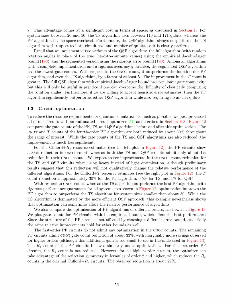
7. This advantage comes at a significant cost in terms of space, as discussed in Section 1. Forsystem sizes between 20 and 50, the TS algorithm uses between 116 and 171 qubits, whereas thePF algorithm has no space overhead. Furthermore, the QSP algorithm always outperforms the TSalgorithm with respect to both circuit size and number of qubits, so it is clearly preferred.

Recall that we implemented two variants of the QSP algorithm: the full algorithm (with randomrotation angles in place of the true, hard-to-compute values) using the empirical Jacobi-Angerbound (193), and the segmented version using the rigorous error bound (190). Among all algorithmswith a complete implementation and a rigorous accuracy guarantee, the segmented QSP algorithmhas the lowest gate counts. With respect to the cnot count, it outperforms the fourth-order PFalgorithm, and even the TS algorithm, by a factor of at least 5. The improvement in the T count isgreater. The full QSP algorithm with empirical Jacobi-Anger bound has even lower gate complexity,but this will only be useful in practice if one can overcome the difficulty of classically computingthe rotation angles. Furthermore, if we are willing to accept heuristic error estimates, then the PFalgorithm significantly outperforms either QSP algorithm while also requiring no ancilla qubits.

I.3 Circuit optimization

To reduce the resource requirements for quantum simulation as much as possible, we post-processedall of our circuits with an automated circuit optimizer [57] as described in Section E.3. Figure 12compares the gate counts of the PF, TS, and QSP algorithms before and after this optimization. Thecnot and T counts of the fourth-order PF algorithm are both reduced by about 30% throughoutthe range of interest. While the gate counts of the TS and QSP algorithms are also reduced, theimprovement is much less significant.

For the Clifford+Rz resource estimates (see the left plot in Figure 12), the PF circuits showa 33% reduction in cnot count, whereas both the TS and QSP circuits admit only about 1%reduction in their cnot counts. We expect to see improvements in the cnot count reduction forthe TS and QSP circuits when using heavy instead of light optimization, although preliminaryresults suggest that this reduction will not qualitatively change the relative performance of thedifferent algorithms. For the Clifford+T resource estimates (see the right plot in Figure 12), the Tcount reduction is approximately 30% for the PF algorithm, 0.5% for TS, and 1% for QSP.

With respect to cnot count, whereas the TS algorithm outperforms the best PF algorithm withrigorous performance guarantees for all system sizes shown in Figure 12, optimization improves thePF algorithm to outperform the TS algorithm for system sizes smaller than about 30. While theTS algorithm is dominated by the more efficient QSP approach, this example nevertheless showsthat optimization can sometimes affect the relative performance of algorithms.

We also compare the optimization of PF algorithms of different orders, as shown in Figure 13.We plot gate counts for PF circuits with the empirical bound, which offers the best performance.Since the structure of the PF circuit is not affected by choosing a different error bound, essentiallythe same relative improvements hold for other bounds as well.

The first-order PF circuits do not admit any optimization in the cnot counts. The remainingPF circuits admit cnot gate count reduction of about 33%, with marginally more savings observedfor higher orders (although this additional gain is too small to see in the scale used in Figure 13).The Rz count of the PF circuits behaves similarly under optimization. For the first-order PFcircuits, the Rz count is not reduced. However, for all higher-order circuits, the optimizer cantake advantage of the reflection symmetry in formulas of order 2 and higher, which reduces the Rz

counts in the original Clifford+Rz circuits. The observed reduction is about 29%.

56

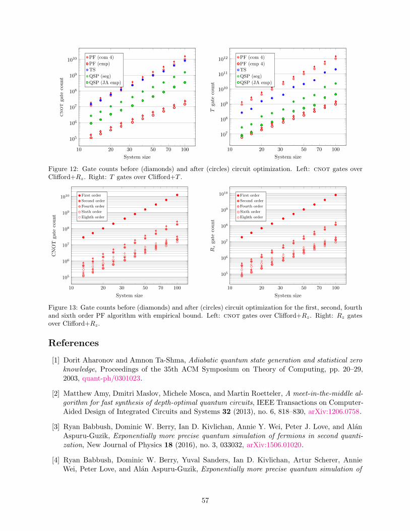
10 100

105

106

107

108

109

1010

20 30 50 70

System size

cnotgate

count

PF (com 4)

PF (emp)TS

QSP (seg)

QSP (JA emp)

10 100

107

108

109

1010

1011

1012

20 30 50 70

System size

Tgate

count

PF (com 4)

PF (emp 4)TS

QSP (seg)

QSP (JA emp)

Figure 12: Gate counts before (diamonds) and after (circles) circuit optimization. Left: cnot gates overClifford+Rz. Right: T gates over Clifford+T .

10 100

105

106

107

108

109

1010

20 30 50 70

System size

CNOT

gate

count

First order

Second order

Fourth order

Sixth order

Eighth order

10 100

105

106

107

108

109

1010

20 30 50 70

System size

Rzgate

count

First order

Second order

Fourth order

Sixth order

Eighth order

Figure 13: Gate counts before (diamonds) and after (circles) circuit optimization for the first, second, fourthand sixth order PF algorithm with empirical bound. Left: cnot gates over Clifford+Rz. Right: Rz gatesover Clifford+Rz.

References

[1] Dorit Aharonov and Amnon Ta-Shma, Adiabatic quantum state generation and statistical zeroknowledge, Proceedings of the 35th ACM Symposium on Theory of Computing, pp. 20–29,2003, quant-ph/0301023.

[2] Matthew Amy, Dmitri Maslov, Michele Mosca, and Martin Roetteler, A meet-in-the-middle al-gorithm for fast synthesis of depth-optimal quantum circuits, IEEE Transactions on Computer-Aided Design of Integrated Circuits and Systems 32 (2013), no. 6, 818–830, arXiv:1206.0758.

[3] Ryan Babbush, Dominic W. Berry, Ian D. Kivlichan, Annie Y. Wei, Peter J. Love, and AlanAspuru-Guzik, Exponentially more precise quantum simulation of fermions in second quanti-zation, New Journal of Physics 18 (2016), no. 3, 033032, arXiv:1506.01020.

[4] Ryan Babbush, Dominic W. Berry, Yuval Sanders, Ian D. Kivlichan, Artur Scherer, AnnieWei, Peter Love, and Alan Aspuru-Guzik, Exponentially more precise quantum simulation of

57

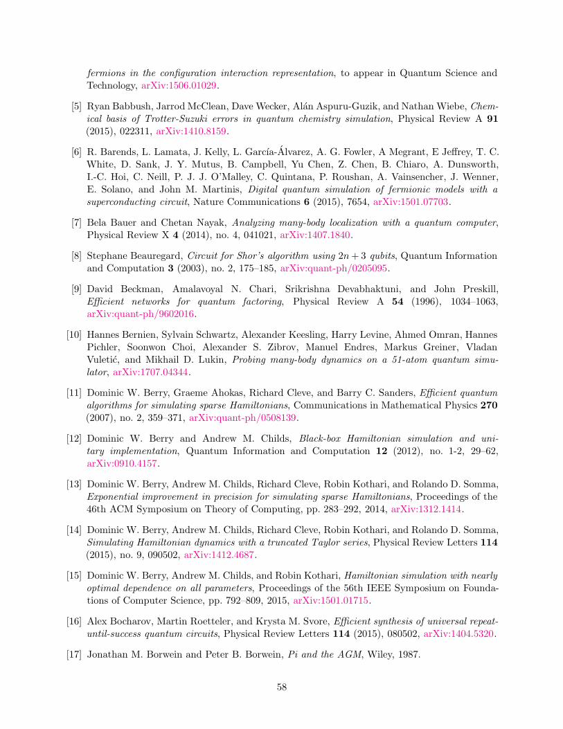
fermions in the configuration interaction representation, to appear in Quantum Science andTechnology, arXiv:1506.01029.

[5] Ryan Babbush, Jarrod McClean, Dave Wecker, Alan Aspuru-Guzik, and Nathan Wiebe, Chem-ical basis of Trotter-Suzuki errors in quantum chemistry simulation, Physical Review A 91

(2015), 022311, arXiv:1410.8159.

[6] R. Barends, L. Lamata, J. Kelly, L. Garcıa-Alvarez, A. G. Fowler, A Megrant, E Jeffrey, T. C.White, D. Sank, J. Y. Mutus, B. Campbell, Yu Chen, Z. Chen, B. Chiaro, A. Dunsworth,I.-C. Hoi, C. Neill, P. J. J. O’Malley, C. Quintana, P. Roushan, A. Vainsencher, J. Wenner,E. Solano, and John M. Martinis, Digital quantum simulation of fermionic models with asuperconducting circuit, Nature Communications 6 (2015), 7654, arXiv:1501.07703.

[7] Bela Bauer and Chetan Nayak, Analyzing many-body localization with a quantum computer,Physical Review X 4 (2014), no. 4, 041021, arXiv:1407.1840.

[8] Stephane Beauregard, Circuit for Shor’s algorithm using 2n+3 qubits, Quantum Informationand Computation 3 (2003), no. 2, 175–185, arXiv:quant-ph/0205095.

[9] David Beckman, Amalavoyal N. Chari, Srikrishna Devabhaktuni, and John Preskill,Efficient networks for quantum factoring, Physical Review A 54 (1996), 1034–1063,arXiv:quant-ph/9602016.

[10] Hannes Bernien, Sylvain Schwartz, Alexander Keesling, Harry Levine, Ahmed Omran, HannesPichler, Soonwon Choi, Alexander S. Zibrov, Manuel Endres, Markus Greiner, VladanVuletic, and Mikhail D. Lukin, Probing many-body dynamics on a 51-atom quantum simu-lator, arXiv:1707.04344.

[11] Dominic W. Berry, Graeme Ahokas, Richard Cleve, and Barry C. Sanders, Efficient quantumalgorithms for simulating sparse Hamiltonians, Communications in Mathematical Physics 270(2007), no. 2, 359–371, arXiv:quant-ph/0508139.

[12] Dominic W. Berry and Andrew M. Childs, Black-box Hamiltonian simulation and uni-tary implementation, Quantum Information and Computation 12 (2012), no. 1-2, 29–62,arXiv:0910.4157.

[13] Dominic W. Berry, Andrew M. Childs, Richard Cleve, Robin Kothari, and Rolando D. Somma,Exponential improvement in precision for simulating sparse Hamiltonians, Proceedings of the46th ACM Symposium on Theory of Computing, pp. 283–292, 2014, arXiv:1312.1414.

[14] Dominic W. Berry, Andrew M. Childs, Richard Cleve, Robin Kothari, and Rolando D. Somma,Simulating Hamiltonian dynamics with a truncated Taylor series, Physical Review Letters 114(2015), no. 9, 090502, arXiv:1412.4687.

[15] Dominic W. Berry, Andrew M. Childs, and Robin Kothari, Hamiltonian simulation with nearlyoptimal dependence on all parameters, Proceedings of the 56th IEEE Symposium on Founda-tions of Computer Science, pp. 792–809, 2015, arXiv:1501.01715.

[16] Alex Bocharov, Martin Roetteler, and Krysta M. Svore, Efficient synthesis of universal repeat-until-success quantum circuits, Physical Review Letters 114 (2015), 080502, arXiv:1404.5320.

[17] Jonathan M. Borwein and Peter B. Borwein, Pi and the AGM, Wiley, 1987.

58

[18] Sergei Bravyi and Alexei Kitaev, Universal quantum computation with ideal Clifford gates andnoisy ancillas, Physical Review A 71 (2005), 022316, arXiv:quant-ph/0403025.

[19] Kenneth R. Brown, Robert J. Clark, and Isaac L. Chuang, Limitations of quantum simulationexamined by simulating a pairing Hamiltonian using nuclear magnetic resonance, PhysicalReview Letters 97 (2006), 050504, arXiv:quant-ph/0601021.

[20] Earl Campbell, Shorter gate sequences for quantum computing by mixing unitaries, PhysicalReview A 95 (2017), 042306.

[21] Yu Chen, C. Neill, P. Roushan, N. Leung, M. Fang, R. Barends, J. Kelly, B. Campbell, Z. Chen,B. Chiaro, A. Dunsworth, E. Jeffrey, A. Megrant, J.Y. Mutus, P.J.J. O’Malley, C.M. Quintana,D. Sank, A. Vainsencher, J. Wenner, T.C. White, Michael R. Geller, A.N. Cleland, and John M.Martinis, Qubit architecture with high coherence and fast tunable coupling, Physical ReviewLetters 113 (2014), 220502, arXiv:1402.7367.

[22] Donny Cheung, Dmitri Maslov, Jimson Mathew, and Dhiraj K. Pradhan, On the design andoptimization of a quantum polynomial-time attack on elliptic curve cryptography, QuantumInformation and Computation 9 (2009), no. 7-8, 610–621, arXiv:0710.1093.

[23] Andrew M. Childs, Quantum information processing in continuous time, Ph.D. thesis, Mas-sachusetts Institute of Technology, 2004.

[24] Andrew M. Childs, On the relationship between continuous- and discrete-time quantum walk,Communications in Mathematical Physics 294 (2010), no. 2, 581–603, arXiv:0810.0312.

[25] Andrew M. Childs and Robin Kothari, Simulating sparse Hamiltonians with star decomposi-tions, Proceedings of the 5th Conference on Theory of Quantum Computation, Communication,and Cryptography (TQC 2010), Lecture Notes in Computer Science, vol. 6519, pp. 94–103,2011, arXiv:1003.3683.

[26] Andrew M. Childs, Dmitri Maslov, Yunseong Nam, Neil J. Ross, and Yuan Su,https://github.com/njross/simcount.

[27] Andrew M. Childs and Nathan Wiebe, Hamiltonian simulation using linear combinations ofunitary operations, Quantum Information and Computation 12 (2012), no. 11-12, 901–924,arXiv:1202.5822.

[28] Shantanu Debnath, Norbert M. Linke, Caroline Figgatt, Kevin A Landsman, Kevin Wright,and Christopher Monroe, Demonstration of a small programmable quantum computer withatomic qubits, Nature 536 (2016), 63–66, arXiv:1603.04512.

[29] Guillaume Duclos-Cianci and David Poulin, Reducing the quantum-computing overhead withcomplex gate distillation, Physical Review A 91 (2015), 042315, arXiv:1403.5280.

[30] Richard P. Feynman, Simulating physics with computers, International Journal of TheoreticalPhysics 21 (1982), no. 6-7, 467–488.

[31] Austin G. Fowler, Simon J. Devitt, and Lloyd C. L. Hollenberg, Implementation of Shor’salgorithm on a linear nearest neighbour qubit array, Quantum Information and Computation4 (2004), 237–251, arXiv:quant-ph/0402196.

59

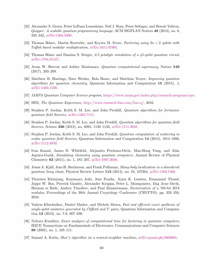
[32] Alexander S. Green, Peter LeFanu Lumsdaine, Neil J. Ross, Peter Selinger, and Benoıt Valiron,Quipper: A scalable quantum programming language, ACM SIGPLAN Notices 48 (2013), no. 6,333–342, arXiv:1304.3390.

[33] Thomas Haner, Martin Roetteler, and Krysta M. Svore, Factoring using 2n + 2 qubits withToffoli based modular multiplication, arXiv:1611.07995.

[34] Thomas Haner and Damian S. Steiger, 0.5 petabyte simulation of a 45-qubit quantum circuit,arXiv:1704.01127.

[35] Aram W. Harrow and Ashley Montanaro, Quantum computational supremacy, Nature 549

(2017), 203–209.

[36] Matthew B. Hastings, Dave Wecker, Bela Bauer, and Matthias Troyer, Improving quantumalgorithms for quantum chemistry, Quantum Information and Computation 15 (2015), 1,arXiv:1403.1539.

[37] IARPA Quantum Computer Science program, https://www.iarpa.gov/index.php/research-programs/qcs.

[38] IBM, The Quantum Experience, http://www.research.ibm.com/ibm-q/, 2016.

[39] Stephen P. Jordan, Keith S. M. Lee, and John Preskill, Quantum algorithms for fermionicquantum field theories, arXiv:1404.7115.

[40] Stephen P. Jordan, Keith S. M. Lee, and John Preskill, Quantum algorithms for quantum fieldtheories, Science 336 (2012), no. 6085, 1130–1133, arXiv:1111.3633.

[41] Stephen P. Jordan, Keith S. M. Lee, and John Preskill, Quantum computation of scattering inscalar quantum field theories, Quantum Information and Computation 14 (2014), 1014–1080,arXiv:1112.4833.

[42] Ivan Kassal, James D. Whitfield, Alejandro Perdomo-Ortiz, Man-Hong Yung, and AlanAspuru-Guzik, Simulating chemistry using quantum computers, Annual Review of PhysicalChemistry 62 (2011), no. 1, 185–207, arXiv:1007.2648.

[43] Jonas A. Kjall, Jens H. Bardarson, and Frank Pollmann, Many-body localization in a disorderedquantum Ising chain, Physical Review Letters 113 (2014), no. 10, 107204, arXiv:1403.1568.

[44] Thorsten Kleinjung, Kazumaro Aoki, Jens Franke, Arjen K. Lenstra, Emmanuel Thome,Joppe W. Bos, Pierrick Gaudry, Alexander Kruppa, Peter L. Montgomery, Dag Arne Osvik,Herman te Riele, Andrey Timofeev, and Paul Zimmermann, Factorization of a 768-bit RSAmodulus, Proceedings of the 30th Annual Cryptology Conference (CRYPTO), pp. 333–350,2010.

[45] Vadym Kliuchnikov, Dmitri Maslov, and Michele Mosca, Fast and efficient exact synthesis ofsingle-qubit unitaries generated by Clifford and T gates, Quantum Information and Computa-tion 13 (2013), no. 7-8, 607–630.

[46] Noboru Kunihiro, Exact analyses of computational time for factoring in quantum computers,IEICE Transactions on Fundamentals of Electronics, Communications and Computer Sciences88 (2005), no. 1, 105–111.

[47] Samuel A. Kutin, Shor’s algorithm on a nearest-neighbor machine, arXiv:quant-ph/0609001.

60

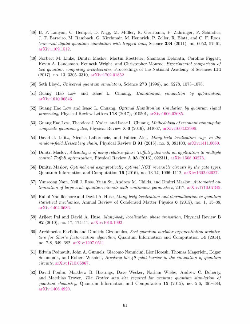
[48] B. P. Lanyon, C. Hempel, D. Nigg, M. Muller, R. Gerritsma, F. Zahringer, P. Schindler,J. T. Barreiro, M. Rambach, G. Kirchmair, M. Hennrich, P. Zoller, R. Blatt, and C. F. Roos,Universal digital quantum simulation with trapped ions, Science 334 (2011), no. 6052, 57–61,arXiv:1109.1512.

[49] Norbert M. Linke, Dmitri Maslov, Martin Roetteler, Shantanu Debnath, Caroline Figgatt,Kevin A. Landsman, Kenneth Wright, and Christopher Monroe, Experimental comparison oftwo quantum computing architectures, Proceedings of the National Academy of Sciences 114

(2017), no. 13, 3305–3310, arXiv:1702.01852.

[50] Seth Lloyd, Universal quantum simulators, Science 273 (1996), no. 5278, 1073–1078.

[51] Guang Hao Low and Isaac L. Chuang, Hamiltonian simulation by qubitization,arXiv:1610.06546.

[52] Guang Hao Low and Isaac L. Chuang, Optimal Hamiltonian simulation by quantum signalprocessing, Physical Review Letters 118 (2017), 010501, arXiv:1606.02685.

[53] Guang Hao Low, Theodore J. Yoder, and Isaac L. Chuang,Methodology of resonant equiangularcomposite quantum gates, Physical Review X 6 (2016), 041067, arXiv:1603.03996.

[54] David J. Luitz, Nicolas Laflorencie, and Fabien Alet, Many-body localization edge in therandom-field Heisenberg chain, Physical Review B 91 (2015), no. 8, 081103, arXiv:1411.0660.

[55] Dmitri Maslov, Advantages of using relative-phase Toffoli gates with an application to multiplecontrol Toffoli optimization, Physical Review A 93 (2016), 022311, arXiv:1508.03273.

[56] Dmitri Maslov, Optimal and asymptotically optimal NCT reversible circuits by the gate types,Quantum Information and Computation 16 (2016), no. 13-14, 1096–1112, arXiv:1602.02627.

[57] Yunseong Nam, Neil J. Ross, Yuan Su, Andrew M. Childs, and Dmitri Maslov, Automated op-timization of large-scale quantum circuits with continuous parameters, 2017, arXiv:1710.07345.

[58] Rahul Nandkishore and David A. Huse, Many-body localization and thermalization in quantumstatistical mechanics, Annual Review of Condensed Matter Physics 6 (2015), no. 1, 15–38,arXiv:1404.0686.

[59] Arijeet Pal and David A. Huse, Many-body localization phase transition, Physical Review B82 (2010), no. 17, 174411, arXiv:1010.1992.

[60] Archimedes Pavlidis and Dimitris Gizopoulos, Fast quantum modular exponentiation architec-ture for Shor’s factorization algorithm, Quantum Information and Computation 14 (2014),no. 7-8, 649–682, arXiv:1207.0511.

[61] Edwin Pednault, John A. Gunnels, Giacomo Nannicini, Lior Horesh, Thomas Magerlein, EdgarSolomonik, and Robert Wisnieff, Breaking the 49-qubit barrier in the simulation of quantumcircuits, arXiv:1710.05867.

[62] David Poulin, Matthew B. Hastings, Dave Wecker, Nathan Wiebe, Andrew C. Doherty,and Matthias Troyer, The Trotter step size required for accurate quantum simulation ofquantum chemistry, Quantum Information and Computation 15 (2015), no. 5-6, 361–384,arXiv:1406.4920.

61

[63] Sadegh Raeisi, Nathan Wiebe, and Barry C. Sanders, Quantum-circuit design for efficientsimulations of many-body quantum dynamics, New Journal of Physics 14 (2012), 103017,arXiv:1108.4318.

[64] Markus Reiher, Nathan Wiebe, Krysta M. Svore, Dave Wecker, and Matthias Troyer, Eluci-dating reaction mechanisms on quantum computers, Proceedings of the National Academy ofSciences 114 (2017), no. 29, 7555–7560, arXiv:1605.03590.

[65] Martin Roetteler, Michael Naehrig, Krysta M. Svore, and Kristin Lauter, Quantum resourceestimates for computing elliptic curve discrete logarithms, arXiv:1706.06752.

[66] Neil J. Ross and Peter Selinger, Optimal ancilla-free Clifford+T approximation of z-rotations,Quantum Information and Computation 16 (2016), no. 11-12, 901–953, arXiv:1403.2975.

[67] Michael Schreiber, Sean S. Hodgman, Pranjal Bordia, Henrik P. Luschen, Mark H. Fischer,Ronen Vosk, Ehud Altman, Ulrich Schneider, and Immanuel Bloch, Observation of many-body localization of interacting fermions in a quasirandom optical lattice, Science 349 (2015),no. 6250, 842–845, arXiv:1501.05661.

[68] M. Serbyn, M. Knap, S. Gopalakrishnan, Z. Papic, N. Y. Yao, C. R. Laumann, D. A. Abanin,M. D. Lukin, and E. A. Demler, Interferometric probes of many-body localization, PhysicalReview Letters 113 (2014), no. 14, 147204, arXiv:1403.0693.

[69] Vivek V. Shende, Stephen S. Bullock, and Igor L. Markov, Synthesis of quantum-logic circuits,IEEE Transactions on Computer-Aided Design of Integrated Circuits and Systems 25 (2006),no. 6, 1000–1010, arXiv:quant-ph/0406176.

[70] Jacob Smith, Aaron Lee, Philip Richerme, Brian Neyenhuis, Paul W. Hess, Philipp Hauke,Markus Heyl, David A. Huse, and Christopher Monroe, Many-body localization in a quan-tum simulator with programmable random disorder, Nature Physics 12 (2016), 907–911,arXiv:1508.07026.

[71] Rolando Somma, Gerardo Ortiz, James E. Gubernatis, Emanuel Knill, and RaymondLaflamme, Quantum algorithms for fermionic simulations, Physical Review A 64 (2002),022319, arXiv:cond-mat/0012334.

[72] Rolando Somma, Gerardo Ortiz, James E. Gubernatis, Emanuel Knill, and RaymondLaflamme, Simulating physical phenomena by quantum networks, Physical Review A 65 (2002),042323, arXiv:quant-ph/0108146.

[73] Chao Song, Kai Xu, Wuxin Liu, Chui ping Yang, Shi-Biao Zheng, Hui Deng, Qiwei Xie,Keqiang Huang, Qiujiang Guo, Libo Zhang, Pengfei Zhang, Da Xu, Dongning Zheng, XiaoboZhu, H. Wang, Y.-A. Chen, C.-Y. Lu, Siyuan Han, and Jian-Wei Pan, 10-qubit entanglementand parallel logic operations with a superconducting circuit, Physical Review Letters 119 (2017),180511, arXiv:1703.10302.

[74] Masuo Suzuki, General theory of fractal path integrals with applications to many-body theoriesand statistical physics, Journal of Mathematical Physics 32 (1991), no. 2, 400–407.

[75] Yasuhiro Takahashi and Noboru Kunihiro, A quantum circuit for Shor’s factoring algorithmusing 2n + 2 qubits, Quantum Information and Computation 6 (2006), no. 2, 184–192.

62

[76] Dave Wecker, Bela Bauer, Bryan K. Clark, Matthew B. Hastings, and Matthias Troyer, Gatecount estimates for performing quantum chemistry on small quantum computers, Physical Re-view A 90 (2014), 022305, arXiv:1312.1695.

[77] Dave Wecker, Matthew B. Hastings, Nathan Wiebe, Bryan K. Clark, Chetan Nayak, andMatthias Troyer, Solving strongly correlated electron models on a quantum computer, PhysicalReview A 92 (2015), 062318, arXiv:1506.05135.

[78] Jiehang Zhang, Guido Pagano, Paul W. Hess, Antonis Kyprianidis, Patrick Becker, HarveyKaplan, Alexey V. Gorshkov, Zhe-Xuan Gong, and Christopher Monroe, Observation of amany-body dynamical phase transition with a 53-qubit quantum simulator, arXiv:1708.01044.

63